the cadastral-based expert dasymetric system - lehman college

Cartography and Geographic Information Science, Vol. 34, No. 2, 2007, pp. 77-102

Mapping Population Distribution in the Urban Environment: The Cadastral-based Expert

Dasymetric System (CEDS)

Juliana Astrud Maantay, Andrew R. Maroko, and Christopher Herrmann

ABSTRACT: This paper discusses the importance of determining an accurate depiction of total population and specific sub-population distribution for urban areas in order to develop an improved “denominator,” which would enable the calculation of more correct rates in GIS analyses involving public health, crime, and urban environmental planning. Rather than using data aggregated by arbitrary administrative boundaries such as census tracts, we use dasymetric mapping, an areal interpolation method using ancillary information to delineate areas of homogeneous values. We review previous dasymetric mapping techniques (which often use remotely sensed land-cover data) and contrast them with our technique, Cadastral-based Expert Dasymetric System (CEDS), which is particularly suitable for urban areas. The CEDS method uses specific cadastral data, land-use filters, modeling by expert system routines, and validation against various census enumeration units and other data. The CEDS dasymet-ric mapping technique is presented through a case study of asthma hospitalizations in the Bronx, New York City, in relation to proximity buffers constructed around major sources of air pollution. The case study shows the impact that a more accurate estimation of population distribution has on a current environmental justice and health disparities research project, and the potential of CEDS for other GIS applications.

KEYWORDS: Dasymetric, geographic information systems, cadastral maps, areal interpolation, areal weighting, expert systems, thematic maps, asthma, New York City

What is Dasymetric Mapping?

Dasymetric mapping refers to a pro-cess of disaggregating spatial data to a finer unit of analysis, using additional

(or “ancillary”) data to help refine locations of population or other phenomena (Mennis 2003). This disaggregation process will result in areas of homogeneity that take into account (and more closely resemble) the actual phenomena being modeled, rather than areal units based on administrative or other arbitrary boundaries. Although it is generally used to get better results for actual locations of population, dasymetric mapping theoretically can be used to disaggre-

gate any quantitative variable that is aggregated by geographic units, such as administrative divi-sions including census enumeration units, ZIP codes, counties, and police precincts; or environ-mental districts, including watersheds, wetlands, or flood plains.

The locations of census tract boundaries, ZIP code postal zones, or any other administrative boundaries, do not necessarily relate to the underlying phenomena, having been created arbitrarily or to suit other governmental purposes. Population totals within a given areal zone are assumed to be distributed evenly throughout the zone, when in fact population distribution is generally much more heterogeneous (Wu

Juliana Astrud Maantay, Associate Professor, Urban Environmental Geography, Director of GISc Program, Lehman College, City University of New York, Environmental, Geographic, and Geological Sciences Department, 250 Bedford Park Blvd. West, NY 10468. Ph: (718) 960-8574; Fax: (718) 960-8584. E-mail: <juliana.maantay@lehman,cuny.edu>; <[email protected]>. City University of New York Graduate Center, Earth and Environmental Sciences Ph.D. Program. Lehman College, City University of New York, Department of Health Sciences, Public Health Graduate Program. Andrew R. Maroko, Lehman College, City University of New York, Department of Environmental, Geographic, and Geological Sciences; and Geographic Information Sciences Program. City University of New York Graduate Center, Earth and Environmental Sciences Ph.D. Program. Christopher Herrmann, John Jay College of Criminal Justice, City University of New York; and New York City Police Department.

78 Cartography and Geographic Information Science

et al. 2005). This creates errors when trying to establish accurate rates for GIS analyses pertaining to health studies, crime patterns, hazard/risk assessment, land-use planning, or environmental impacts, among others, that rely on a smaller unit of analysis than the original zones. Examples of this are impact buffers that intersect the census enumeration unit, or a different set of zones altogether that do not coincide with the original set (e.g., overlaying data from units with non-coincident boundaries and/or overlapping spatial units such as census tracts and police precincts or health districts).

Although dasymetric mapping has been in use since at least the early 1800s, it has never achieved the ubiquity of other types of thematic mapping, and thus the means of producing dasymetric maps have never been standardized and codified the way other types of thematic mapping techniques have been (Eicher and Brewer 2001; Slocum 1999). Therefore, dasymetric methods remain highly subjective, with inconsistent criteria. The reason for this relative lack of popularity and the paucity of standard methodology surely lies at least partially in the difficulty inherent in constructing dasymetric maps, and until recently, the difficulties in obtaining the necessary data, as well as access to the computer power required to generate them.

The dasymetric method we have developed uses census data in conjunction with cadastral (tax lot) data in order to create a more precise picture of where people actually live. Using data aggregated by census enumeration units assumes that population is distributed homogeneously throughout the unit, which is rarely the case in reality. This assumption of homogeneity results in incorrect denominators (counts of the total population affected by the phenomena being investigated) being used to calculate rates (disease, crime, impacted populations, and so forth), which in turn results in either an under- or overestimation of the risk or its occurrence.

The proposed Cadastral-based Expert Dasymetric System (CEDS) leads to a better estimation of population (and potentially of specific sub-populations), and thus to a more complete understanding of the spatial distribution and patterns of disease, crime, hazard, exposure, and other issues. Following our review below of some of the most frequently-used dasymetric methods, we will describe the CEDS method, and then present it through an example of mapping population distribution in New York City, by comparing choropleth

mapping, areal interpolation, filtered areal weighting, and CEDS. We then further illustrate CEDS through a case study showing how the CEDS method improves an environmental health justice analysis of asthma in the Bronx.

Historical Background of Dasymetric MappingMany early cartographic endeavors were con-cerned predominantly with producing maps intended for navigational and exploration purposes; these required furthering our abili-ties to observe and measure the physical world with increasing levels of precision (Hall 1994). Technical advancements in instrument design and geometric theory made these more precise maps possible, and they generally portrayed tangible aspects of the physical world, such as areal sizes of geographic units, topography, tem-peratures, and sea depths (Dorling and Fairbairn 1997). Maps depicting social, cultural, or eco-nomic aspects of the world are termed thematic maps—those showing a particular “theme,” such as poverty levels, disease rates, or the flow of migration. Thematic maps (also called statistical maps, if depicting a quantitative data theme) are generally of more recent vintage (Dent 1999). One of the earliest known examples of a the-matic map is the mathematician Baron Pierre Charles Dupin’s 1826 unclassed choropleth map showing illiteracy levels in each of the admin-istrative departements comprising France, where the areal units were shaded in greytones, with the darker tones indicating a higher illiteracy rate (Robinson 1982: p. 232).

Although no real typology of thematic maps had been developed at that time, most of the major types of statistical graphics and thematic maps as we know them today originated in the first half of the 19th century as a means to visualize quantitative information. As national governmental powers grew and consolidated in this time period, the need arose for a more detailed view of the popu-lation and associated data related to population, such as numbers about health, crime, education, poverty, and economics (Koch 2005). Statistical mapping met this need, and for the first time, the types of data needed to produce these maps were collected and made available.

Milestones in dasymetric mapping would have to include Scrope’s 1833 classed population den-sity map of the world, which used a rudimentary dasymetric technique (Scrope 1833). However, the Russian geographer, Semenov-Tyan-Shansky (1827-

Vol. 34, No. 2 79

1914), who studied under von Humboldt and Ritter in Berlin and advanced the use of statistical map-ping, has often been credited with inventing the dasymetric map (Bielecka 2005). The American geographer, John Kirtland Wright (1891-1969), who was perhaps the first person to publish a paper on dasymetric mapping in an English-language journal, stated that dasymetric means “density measuring.” His 1936 paper is generally consid-ered the seminal paper on dasymetric mapping, in which he extolled the virtues of the dasymetric map over the choropleth map (Wright 1936). He also coined the term “choropleth” (value-by-area) map, although choropleth maps were in use since at least the early nineteenth century.

Today, the need for visualization of population data is even more necessary, not just for descrip-tive purposes—to show the geographic extent and density of populations—but also for spatial analyti-cal and predictive modeling purposes, in order to inform risk assessments and public policy formation on many urban issues (Gregory 2000; Moon and Farmer 2001; Poulsen and Kennedy 2004; Sleeter, 2004). The more traditional thematic mapping techniques may not be sufficient to display and analyze these data. Choropleth mapping, one of the most widely used thematic map techniques today, has many benefits, but it is lacking in a few important ways. The choropleth method is familiar, and easily comprehended and interpreted by the map reader, and it is comparatively straightforward to compute. For instance, population density for a given enumeration unit can be normalized by dividing the total population by the areal measure-ment of the unit. However, drawbacks include the Modifiable Areal Unit Problem (MAUP), which describes the phenomenon that, by modifying areal boundaries and/or the level of data aggre-gation, the results of the spatial analysis will be substantially different (Openshaw 1984).

Choropleth maps also have a propensity to gen-eralize the high and low values within a given enu-meration unit, removing the spatial heterogeneity in the data values. Additionally, choropleth maps depict abrupt changes at the boundaries of enu-meration units, which are based on the existence of artificially defined boundaries, and not boundar-ies defined by the reality of the data. Dasymetric maps can be subject to abrupt boundary changes as well, but “these transitions are a better reflec-tion of the true underlying geography of the area than the transitions in choroplethic maps, which are artifacts partially attributable to the arbitrary delineation of areal boundaries. This limitation of dasymetric mapping is offset by the technique’s

better visualization of population patterns, due to the high degree of spatial disaggregation that can be achieved” (Holt et al. 2004, p. 104).

Methods and Data Used in Dasymetric MappingTransferring data from one set of geographic zones or districts to another set of non-coinci-dent zones is often necessary in spatial analysis. For instance, we might have data on the number of people living within a certain census tract but need to estimate the number of people in a smaller area within the tract, or an area that includes only part of that tract and part of other tracts. We may be interested in population or other data at a watershed level and only have population data available at the census enu-meration units. “In any one study, several dif-ferent types of data may be collected at differing scales and resolutions, at different spatial loca-tions, and in different dimensions” (Gotway and Young 2002, p. 632).

A typical example of this is the problem encoun-tered when conducting spatial analysis on histori-cal census data from various time periods, with each temporally different attribute data set using different spatial data as well, because the tract boundaries used to aggregate the attribute data may change with each census period (Gregory 2000). How can one determine the number of people living in only a portion of an area for which data have been aggregated, or in an area for which the zones containing the data of interest do not coincide among various data layers?

Several methods of disaggregating population data are discussed below: weighted areal interpolation; filtered weighted areal interpolation; the use of land use/land cover as ancillary data for filtering; three-class and limiting variable methods; “image texture” method; statistical approaches, such as regression-based methods; heuristic sampling; kernel density surface using weighted census centroids; the use of other types of ancillary data sets, such as street-weighted interpolation; and the proposed CEDS method.

Areal InterpolationA common method for calculating disaggre-gated population values is areal interpolation. This is defined as “the transfer of data from one set (source units) to a second set (target units) of overlapping, non-hierarchical, areal units (Langford et al. 1991, p. 56). Areal interpola-tion is closely related to dasymetric mapping


of population densities (Holt et al. 2004). The main difference between areal interpolation and dasymetric mapping is that with the later approach, the data are not re-aggregated into a desired enumeration unit as they are with areal interpolation (Eicher and Brewer 2001).

A simple method of areal interpolation is to weight the variable’s values by a ratio derived from the relative areal measurements of the two types of zones (source and target) (Goodchild and Lam 1980). Areal weighting is based on the assumption that population (or another variable) is distributed homogeneously throughout the “source” zone (the original unit of data aggregation). The amount of population estimated to be in the intersecting zone (or “target” zone) is assumed to be proportional to the amount of area in the source zone versus the target zone. The ratio of area of source zone to target zone is then applied to population in the source zone to yield the population total in the target zone

In a study of areal interpolation for socioeco-nomic data, Goodchild et al. (1993) looked at a typical problem of spatial analysis using non-coincident areal units, namely the 58 counties of California (the source zones) and the state’s 12 major hydrological basins (the target zones). The boundaries of the two sets of spatial units were, for the most part, incompatible. The socioeconomic data are available on the county level, but data connected with water issues are collected based on the hydrologic basin units that correspond to major watershed boundaries. In order to conduct a major economic impact study of water usage and policy, variables such as employment, income, and population had to be transferred from the county spatial units to the hydrological regions. Goodchild et al. (1993) used direct areal weighting to accomplish this, assuming that densities in the source zones (the counties) were uniform. When later comparing the results of the areal weight-ing method with other methods using statistical approaches, they found that areal weighting had a much higher mean percentage error than did the other methods.

One of the major sources of error in the areal weighting method is that, typically, population is not distributed evenly throughout a geographic unit. Many things may make this so: large areas of the zone may be uninhabitable due to the existence of parks, water bodies, and industrial area; or, the zone may be comprised of very different housing types—one part of the zone may have high-rise housing projects, while another part contains lower-density single family homes. Therefore, having a

better way of disaggregating the data—rather than assuming homogeneity—should help give more accurate population totals for the target areas.

Filtered Areal Weighting (Binary Method) Many previous dasymetric mapping studies have used areal weighting as a starting point, adding the additional step of filtering the data using an ancillary data set (Flowerdew and Green 1989; Goodchild and Lam 1980; Holt et al. 2004). The ancillary data very often consist of land-use or land-cover data that indicate where the uninhab-itable areas are, then exclude these areas and re-distribute the population in the remaining areas. The simplest of these methods has been termed the “binary” method (Eicher and Brewer 2001), which uses remotely sensed data or land-cover/land-use polygon data as a filter or mask to elim-inate the areas deemed to be uninhabitable. It is considered binary because land is designated as either inhabited or uninhabited. Examples of uninhabited land are parks, water bodies, cem-eteries, industrial parks, and so forth.

In a study of burglaries in central Massachusetts, Poulsen and Kennedy (2004) wanted to show the distribution of residential burglaries as a rate, with the number of housing units as the denominator and the number of residential burglaries as the numerator. Using the housing unit data in the census led to misleading rates, since the housing units were not distributed evenly throughout the census blocks. Using the residential land use and zoning layer as a mask, the non-residential areas were removed from the equation, and rates could be based on the potential burglary targets (the housing units) and the number of burglaries in the municipality. “Land-use data are classified by assigning a value of 1 to residential cells and 0 to all other cells to create a mask. This mask is used to isolate residential areas within the municipality. The source and target zones are multiplied by the mask to remove cells that do not fall into residential areas (Poulsen and Kennedy 2004, p. 255).

Although results of the filtered areal weighting are generally an improvement over simple areal weighting, there are still considerable deficiencies in this method. For instance, all residential areas do not have the same density of housing units or population, but filtered areal weighting assumes that all residential areas are homogeneous with respect to density. Additionally, non-residentially zoned areas often have population, too, which is totally eliminated in the purely binary approach. Some of the methods discussed below offer

Vol. 34, No. 2 81

further refinements to filtered areal weighting, taking it from a binary model to a more nuanced approach, which results in a more realistic depiction of densities typically encountered in the real world.

Land Use/Land Cover as Ancillary DataAlthough land-use polygon (vector) data sets have occasionally been used as the filtering layer (e.g., Bielecka 2005; Poulsen and Kennedy 2004), most dasymetric studies have used satel-lite data (raster data format) to determine the locations of uninhabited areas, and/or to classify inhabited areas by population density (Holloway et al. 1999; Langford and Unwin 1994; Mennis 2003; Sleeter 2004). For instance, using Digital Terrain Elevation Data (DTED) for global cover-age of roads and slopes and USGS’ Global Land Cover Characteristics derived from Advanced Very High Resolution Radiometry (AVHRR) satellite imagery as indicators of population distribution, researchers have created a global population database known as LandScan, with a spatial resolution of under one kilometer.

“LandScan…is the finest global population data (<1 km resolution) ever produced and is several orders of magnitude more spatially refined than some of the previously available global popu-lation datasets,” (Bhaduri et al. 2002, p. 34). While this broad-brush approach may be neces-sary and sufficient when working with very small scales, such as continents, countries, states, or large regions, it is less satisfactory when working with metropolitan areas, counties, local commu-nities, or other relatively large-scale areas.

In highly urbanized areas, land-cover data derived from satellites may not yield precise enough results to get a true picture of population density, due to limitations in available pixel resolution and intra-pixel heterogeneity of urban areas (Forster 1985). Additionally, using the extent of impervious surfaces or other physical or morphological variables as interpreted from satellite data as a proxy for degree of urbanization or urban development can result in misclassification for population density classes. For instance, industrial and commercial areas usually have large extents of impervious surfaces and thus are classified as highly urbanized. Using this interpretation of satellite imagery, these areas are counted as areas of high population density, which they usually are not.

Where higher-resolution satellite data are available, such as in the United States, LandScan is being developed at a 90-meter

resolution (Bhaduri et al. 2002). But even at this resolution, densely settled urban areas may have too much within-pixel heterogeneity to pin-point population distribution with the accuracy necessary for fine-grained analysis. For instance, 90 meters is approximately the size of a New York City street block (200 linear feet per block face), and within one block there can be several very different land uses, as well as various densities of residential dwellings, from single-family homes to multi-family apartment buildings, all of which would have very different population densities but would show as one value in the image.

Recent advances in remote sensing have yielded very high spatial resolution images, with pixels representing one meter or less on the ground. But even with these data, difficulties of correctly assigning population to land-use/land-cover classes abound. Although one can interpret the images as to the locations of impervious surfaces, and perhaps even show building footprints, the image does not easily reveal the height of the buildings or how many dwelling units are contained within each structure, or indeed, whether the structure is residential, commercial, or industrial. For the purposes of many health, crime, or environmental analyses, this ambiguity makes even high-resolution data insufficient.

In their excellent review of methods to estimate population using GIS and remote sensing, Wu et al. (2005) discuss the method of estimating the population of an area by multiplying the total number of dwelling units with the number of persons normally living in a dwelling unit. They say that the number of dwelling units in an area may be estimated from high-resolution remote sensing images. However, this would really only work when the environment is comprised of single family homes, each constituting one dwelling unit; it is unlikely to be accurate when dealing with mid- or high-rise residential buildings having many dwelling units per floor, which constitute the majority of residences in many dense urban areas. Although with the increased use of LIDAR it may be feasible to estimate building height, it is still unlikely that this will result in an accurate accounting of the number of dwelling units per floor.

The main drawbacks of using remotely sensed images for the purposes of constructing an accurate population map are summed up by Moon and Farmer (2001): “[s]atellite imagery is also relatively expensive, requires significant data storage, processing, and computational capacity, and suffers from weaknesses in classification


routines used to separate residential areas from nonresidential areas” (Moon and Farmer 2001, p. 42).

Three-Class and Limiting Variable MethodsFurther refinements of the binary method include the three-class (or class percent) method and the limiting variable method (Eicher and Brewer 2001). In the three-class method, percentages are applied to each of the three (or more) major land-use categories for that area, representing the percentage of population (or another variable) that is likely to be contained within that land use, per district. For instance, if the three major land-use categories are said to be urban, agricultural/woodland/exurban, and forested, the percentages might be 70 percent, 20 percent, and 10 percent, respectively. In this case, we would expect that within a given geographical unit, such as a county, 70 percent of the population would be allocated to the polygons (or grid cells, if using raster data) determined to be in the “urban” category, 20 percent of the population would be allocated to the “agricultural” polygons, and so forth. These percentage numbers will vary depending on the location of the area of interest, and are subject to perceived local conditions and arbitrariness of the analyst.

The assigning of the percentages is fairly subjective and not based on statistical evidence. Furthermore,

“a major weakness of the three-class method is that it does not account for the area of each particular land use within each county. A worst-case scenario would result for a county that had only one or two small urban polygons [or grid cells, if using raster-based data]. These polygons would still receive 70 percent of the [county-wide] data… causing the urban areas in that county to have unusually high densities and the other land-use areas to have lower densities” (Eicher and Brewer 2001, p. 130). The assumption behind this method is that “each land-use class has a characteristic population density. The problem with this approach is that although the difference between land-use classes is recognized, the differences within a land-use class are ignored. Not all residential areas have the same population density, as evidenced by the contrast between detached housing and multiple-unit housing” (Liu et al. 2006, p. 188).

The limiting variable method expands upon the three-class method by setting threshold density limits for population assigned to the various categories of land-use polygons (or grid cells). The data are distributed within each unit

by simple areal weighting, and, subsequently, the limiting thresholds are applied. Upper limits on densities are established using data from geographic units having only one class of land use within their boundaries. The data for all such units are ranked, and a certain percentile is selected to be the limiting threshold for that class. If any land-use polygon exceeds the established threshold for its class of land use, the excessive population is “removed” and redistributed to the other land-use polygons within that geographic unit. A problem with this method (as well with as the three-class method) is that although it is assumed that there are significant differences in density between classes of land use there are likely also to be significant differences within any given land-use class, and this method does not address those intra-land-use class differences. Additionally, if the sample size of the mono-class geographic units used to determine the threshold number is small, and “the within-class population density variance is high, the low number of samples may yield a non-representative estimate of [the population density for that class], and hence an inaccurate dasymetric map” (Mennis and Hultgren 2005, p. 7).

“Image Texture” MethodAnother method using very high spatial reso-lution satellite images, such as the Ikonos one meter imagery, estimates population based on image “texture.” Rather than using categorical land use as a surrogate for population density, as in the methods discussed above, this method examines the correlation between census popu-lation density and image texture. Spatial units called “Homogeneous Urban Patches” (HUP) are obtained by “using texture-based image segmentation which maximizes between-patch differences while minimizing within-patch dif-ferences” (Liu et al. 2006, p. 188).

Unlike other spatial units used in population estimation from remotely sensed images, such as the kernel window or the pixel, HUPs consist of realistic, irregularly shaped units, each having a similar within-unit characterization. Spatial met-rics are used to characterize the texture of each HUP, taking into account such factors as variety and abundance of patch types within each HUP; the spatial arrangement, position, or orientation of patches within each HUP; patch density, con-nectivity, and contagion of patches; and degree of fragmentation—similar to analyses conducted in landscape ecology. Of the nine spatial metrics examined in the study by Liu et al. (2006), only

Vol. 34, No. 2 83

three showed significant correlation: percentage of built-up area, percentage of vegetation in the area, and the patch density of the built-up area. Although some correlation between image texture and population density was demonstrated, it is not high enough to provide reliable estimates of population distribution. “This research shows that remote sensing images can indeed help to estimate population density; however, the correlation may not be strong enough for empirical applications” (Liu et al. 2006, p. 195).

Statistical Approaches—Regression-based AnalysesOther researchers have used more statistical approaches to dasymetric mapping, such as area-to-point spatial interpolation (Kyriakidis 2004), as well as regression-based techniques to correlate population density classes with land-use/land-cover data (Bielecka 2005; Flowerdew et al. 1991; Flowerdew and Green 1992, 1994; Goodchild et al. 1993; Langford et al. 1991). Bielecka recently (2005) produced a dasymetric map of northeastern Poland by using the “modi-fying areal weighted method” which assumes that the ratio between the population density of two land-cover categories is the same for any given commune (local administrative division). The ancillary data was the CORINE land cover database, a polygon (vector) spatial file derived from visual interpretation of satellite images and composed of 31 classes of land cover in Poland. A regression model was used to find the relation-ship between land-cover classes and population density in each commune. This resulted in six categories of population density –land use, and coefficients were developed weighting popula-tion to the land-cover category.1 Comparing the modeled population and the population as measured by statistical data shows that they are roughly in agreement. However, the coefficients appear to be too high for urban communes and too low for rural areas. In addition to this poten-tial accuracy issue, regression analyses usually conducted in order to estimate zonal weights are relatively complex compared to traditional dasymetric methods.

Heuristic Sampling MethodIn another recent study of a five-county area in Pennsylvania, Mennis (2003) uses dasymet-ric mapping, areal weighting, and empirical sampling based on satellite data to generate a surface-based representation of population dis-

tribution not reliant on pre-existing areal unit aggregation. This heuristic sampling approach addresses some of the shortcomings of the pre-vious methods; it takes the three-class method to a higher level of accuracy, while reducing some of the inherent subjectivity of that method. The population of each block group was distrib-uted to each grid cell in the population surface based on two factors: 1) the relative difference in population densities among the three urban-ization classes (low, high, and non-urban), and 2) the percentage of total area of each block group occupied by each of the three urbaniza-tion classes (Mennis 2003). Population density values for each urbanization class were sampled empirically, which mitigated the subjectivity of the assignment of a percentage of population to a given ancillary data class (land use or land cover). Area-based weighting addressed the dif-ferences in area among ancillary data classes within a given areal unit. The sampling pro-cess selected all block groups that were entirely contained within each urbanization class, found their total population and area, and calculated their aggregated population density. This frac-tion established for each class was further modi-fied by the amount of area occupied by each class per block group, using an area ratio derived by areal weighting.

Even though Mennis’ study represents an improve-ment over many previous dasymetric mapping methods, the results for dense urban areas are not sufficiently detailed for many urban planning and analysis purposes. The results for the suburban and rural areas are more detailed and accurate than vector maps made from census block group data; however, his results for the highly urbanized core areas do not differ significantly from the vector block group maps that he started with, because

“considerable intra-block group variation exists in urbanization class and, thus, population den-sity” (Mennis 2003). To sum up, intra-block group variation is not revealed for the most urbanized population density class by using this methodol-ogy and data.

Kernel Density Surface from Population-weighted Census CentroidsA number of related surface-generating meth-ods and refinements of these methods are used to model a population surface by kernel density estimation (Bracken and Martin 1989; Martin et al. 2000; Martin 2006). Rather than mapping

1 The coefficients are computed in an iterative way.


population by zones, such as a census enumera-tion district (or census tract in the U.S.), this method entails creating a surface of population density by interpolating population based on the population-weighted enumeration district (ED) centroid, as are available in the United Kingdom census data. A kernel window is moved over the cells containing these centroids, and the popula-tion count at each centroid is distributed to the cells in the kernel window by a distance-decay model. An early iteration of this method had the drawback that the surface population counts did not always add up to the “correct” counts in the census zonal data (Bracken and Martin 1989). This was later revised so that the pycnophylac-tic (volume-preserving) quality was maintained, and the kernel window distributed the counts from each centroid only to cells within the cen-troid’s original zonal boundaries (Martin 2006). Cell sizes ranging from 50 meters to 200 meters were used, although the 200-meter cell was deemed too crude a resolution for most urban EDs. Even the 50-meter cell is often larger than the smallest of the EDs and, therefore, does not adequately represent the nuances of popula-tion distribution within the densest parts of the city, typically composed primarily of small EDs. However, this density surface model reproduces the essential form of population distribution in the city and indicates major non-populated open spaces such as cemeteries, industrial areas, and commercial districts.

Use of Other Types of Ancillary Data— Street-weighted InterpolationAnalyses of urban issues often require very detailed data on population location in order to yield meaningful results. Previous methods relied primarily on land-use/land-cover data, which has not proved to be as fine-grained as necessary for many urban analysis purposes. In another recent study, Reibel and Bufalino (2005) used the street network data (TIGER files from the U.S. Census) to derive weights for interpo-lation for population and housing unit counts for incompatible zone systems in Los Angeles County, California. Building on previous simi-lar work by Ong and Houston (2003) and Xie (1996), they used the street and road grid as a proxy for approximate population and hous-ing unit density surfaces for census tracts in the county. They then conducted an error analysis, comparing the results of the street-weighting method with traditional areal weighting, and found that the street-weighting method offers

a 70 percent improvement over areal-weight-ing for the estimation of the housing unit count variable and a 20 percent improvement for the estimation of the total population count variable. They note, however, that “the street-weighting method appears to reduce errors most com-pared with the area-weighting method in those areas where the lack of population is reflected in the lack of roads and least in those areas (such as industrial areas) with a more developed, but non-residential transportation infrastructure” (Reibel and Bufalino 2005, p. 136).

By using only vector data sets, this method obviates the need for the analyst to be familiar with processing and interpreting remotely sensed images and integrating raster and vector datasets, making dasymetric mapping more accessible to demographers, urban planners, environmental managers, and others for whom vector data sets are typically a more familiar part of their GIS experi-ence than satellite data. This is a real advantage to this method, since heretofore areal weighting methodology was the most frequently used method for those using only vector data sets, and the street-weighting method is a clear improvement over that approach. However, the street-weighting method appears least reliable in the very areas of most concern to urban analysts—the densely settled, heterogeneous urban core areas.

With the Vienna, Austria, metropolitan area as a study area, Weichselbaum et al. (2005) also used street infrastructure as ancillary data, along with very high resolution Earth Observation satellite imagery, to create a “building block” spatial data set. “The road network data are used for building the geometric framework for population allocation by converting the linear road segments to polygons that make up the building blocks. Such building blocks constitute meaningful reference units for the disaggregated population, as they reflect the real-world housing patterns and population dis-tributions” (Weichselbaum et al. 2005).

The population density classes for these build-ing block polygons were derived from satellite images and sampling of representative densities in homogeneous census tracts, similar to Mennis’ (2003) empirical sampling technique, but using five land-use/land-cover categories and four residential population density classes. When comparing the modeled disaggregated population to the original census grid data, the average error found was 12.44 percent. This compares very favorably to the relative error of 102 percent obtained without using the ancillary land-use data. However, even an error margin of 12 percent can obfuscate analyti-

Vol. 34, No. 2 85

cal findings when dealing with very fine-grained and heterogeneous urban areas.

Cadastral-based Expert Dasymetric System (CEDS)Our method of using cadastral data as the ancillary data appears to be an innovative and progressive approach to dasymetric mapping. Cadastral data are used in recording prop-erty boundaries, property ownership, property valuation, and, of course, for the all-important purpose of property tax collection. The type of cadastral-level data used in our CEDS method is commonly available for most urbanized areas in the United States, western Europe, and other more developed areas. The data are usually organized by township, municipality, or county, and, less often, by metropolitan region.

However, in many parts of the world, census and cadastral data may not be readily available, current, or accurate. Baudot (2001) makes the point that for urban areas in less-developed countries, very often there are no census property tax records or city planning data on population to work with, and even when such data are collected, the exponential growth rates of these cities makes the census data obsolete almost immediately. This is why satellite data are most often used for dasymetric map-ping—they are available for almost all parts of the world and are very current. However, “urban environments are often considered too complex to be analyzed by satellite remote sensing, and, indeed, the spatial resolution of current satellite sensors means that they are not particularly well

suited to the task” (Baudot 2001, p. 266). In urban areas where census and cadastral data are available, the CEDS method will be an improvement. For instance, munici-palities where property tax records are linked to a digital spatial database (e.g., most cities and larger towns in the United States), the cadastral data required by the CEDS method will be available. Although these data may not be available to the general public for free, they still tend to be less expensive for the end user than high-resolution remotely sensed images for the equivalent spatial extent.

Comparison of Areal Weighting, Filtered Areal Weighting, and CEDS Dasymetric Mapping: A Hypothetical ExampleThe following diagrams illustrate how the CEDS method of dasymetric map-

ping can be beneficial to health, environmental, crime, risk assessment, and urban planning anal-yses. The diagrams in Figure 1 contrast standard areal weighting interpolation and filtered areal weighting dasymetric (binary) techniques with the cadastral expert dasymetric system (CEDS) method.

The CEDS method differs from other forms of dasymetric mapping because it does not use areal weighting or the binary (filtered areal weight-ing or “punch-out”) method alone. The ancillary data used are not remotely sensed land cover/land use, interpreted to estimated population density classes, but rather very detailed cadastral data, more appropriate to estimating population distribution in hyper-heterogeneous urban areas. The CEDS method also uses an expert system to determine which variable in the cadastral dataset to use as the ancillary data, calculating which ancillary data fits the data best. In this way, each source record within the area of interest can be customized as to the method of disaggregation, which, when validated, yield results that best fit the data.

Using the CEDS method, the modeled population data always preserve the pycnophylactic property, meaning that the estimated (modeled) value of the tract, when re-aggregated, equals the original value of the tract (Tobler 1979). Preservation of the pycnophylactic property is not always achievable with previously used dasymetric methods based on population density classes derived from land-use/land-cover data.

Figure 1. Methodological differences and potential improvement of population estimation of the CEDS method (c), over both filtered areal weighting (b), and simple areal weighting (a).


CEDS Methodology and AnalysisThe strength of the Cadastral-based Expert Dasymetric System (CEDS) methodology is the ability to disaggregate data at high spatial resolution in a densely populated urban envi-ronment such as New York City (NYC). Much of our previous work has involved analyses of hyper-heterogeneous large-scale geographies for health, environmental, and crime studies in the New York City metropolitan area (Clarke and Maantay 2006; Herrmann and Maroko 2006; Maantay 2001, 2002, 2005); Maantay and Strelnick 2003; Maroko and Maantay, 2006, unpublished study). We have found that these sorts of analyses could be greatly improved by the use of more fine-grained spatial data in place of a coarse aggregation of available popu-lation data.

This CEDS method was designed to disaggregate the total population counts from the census block group level (5,733 in NYC) to the tax lot level (847,153 in NYC) using cadastral data. Census block groups, rather than the smaller census blocks, were used in order to avoid data suppression of subpopulations in the latter. The accuracy of these data will ultimately become important when the CEDS method is applied to subpopulations (e.g., Hispanic, non-Hispanic white, non-Hispanic black, Asian, etc.). If the selected subpopulations do not follow the same trends as does the total population and benefit from individualized expert systems, it will be necessary to use the coarser census block group aggregation. However, if the subpopulations do mirror the behavior of the total population, the disaggregation will be performed on census block data to further constrain the calculations and improve accuracy.

The technique uses residential area (RA) and number of residential units (RU) as proxies for population distribution. In other words, it is assumed that where there are more potential living accommodations there will be higher populations. As such, the population in each block group was disaggregated (or redistributed) among the tax lots based on either RA or RU. The proxy unit (RA or RU) used in the disaggregation was indi-vidually determined by an expert system for each geographic unit. The results were then validated against census data and compared to commonly used dasymetric techniques to assess predictive accuracy and possible improvement over other methods.

The CEDS disaggregation of census populations can be compartmentalized into three fundamental

steps: 1) data preparation, 2) dasymetric calcula-tions, and 3) expert system implementation. The discussion of these steps is followed by an evalu-ation of the results.

Data PreparationTwo datasets were used for this process: the 2000 census data (United States Bureau of the Census 2001a, 2001b) and LotInfo (LotInfo, LLC 2001). Decennial census data for New York City was downloaded via www.census.gov. The total population data (SF1, table P001), which are aggregated in a hierarchical fashion (see Table 1), were obtained at the census tract and

census block group levels, with each tract con-taining multiple block groups. LotInfo, a prod-uct of LotInfo, LLC, which combines spatial data from the New York City Department of City Planning (DCP) and attribute information from the Real Property Attribute Data (RPAD) data-base provided by the New York City Department of Finance (DOF), contains exhaustive data at the tax lot level in New York City (e.g., zoning, ownership, building attributes, residential area, and residential units). Although this study was done in New York City, similar data are often available from planning departments of metro-politan areas or urbanized counties.

The goal of the data preparation was to minimize error-inducing anomalies and discrepancies. The data were refined by editing geographic identi-fiers and deleting fields that were not needed so that they would be readily comparable and more efficiently manipulated. Included in this refinement was the exclusion of the Riker’s Island census tract and complimentary block groups and tax lots. Riker’s Island, with one of the highest populations of any tract in the city, is a prison, and as such there is inconsistency in the way this area is handled between the census and the lot data. For this reason, results would have been drastically skewed with its inclusion.

Table 1. Comparison of spatial unit counts in New York City.

Areal Units in New York City

Unit NumberAverage Number of Units per Tract

Census Tracts 2,217 1.00

Census Block Groups 5,733 2.59

Tax Lots 847,153 382.12

Vol. 34, No. 2 87

was aggregated up to the block group and tract levels (see Figure 2). This table was then used to generate a tax lot-level spatial data layer with RU and ARA values aggregated at the tax lot, block group, and tract levels, as well as the census population data at the block group and tract levels. It is important to note that the data which are aggregated to larger areal units are identical for each lot within any given areal unit. In other words, if tax lots “1”, “2”, and “3” are all within tract “A,” they will all share the same tract-level information.

Several dasymetrically derived populations were then calculated. The general equation is solved by multiplying the census population with the ratio of population proxy units thus:

POPl = POPc * Ul / Uc (2)

where:POPl = dasymetrically derived lot-level population;POPc = census population (block group or tract); Ul = the number of proxy units at the tax lot level (RU or ARA); and Uc = the number of proxy units at the census level (RU or ARA per block group or tract).Values were calculated from the block group

and tract census populations using both RU and ARA as the proxy units. The process resulted in four dasymetrically derived population values for each tax lot (tract ARA, tract RU, block group ARA, and block group RU).

Expert System ImplementationThis expert system was designed to determine which proxy unit—number of residential units (RU) or adjusted residential area (ARA)—more

As was already mentioned, residential area (RA) and number of residential units (RU) are important attributes in the CEDS process. Within the lot-level data, the RU variable did not require additional processing; however, there were many instances of missing data values for the RA variable in the original RPAD data from the Department of Finance. As such, a new variable, adjusted residential area (ARA), was created. The adjusted variable is identi-cal to RA in many cases, however when the value for RA is zero and the number of residential units (RU) does not equal zero (i.e., there are residential units but no value for residential area), ARA is defined as the total building area multiplied by the ratio of the number of residential units and the total number of units. The ARA variable can be written as follows:

ARA = M * (BA * RU / TU) + RA

IF RA = 0 AND RU <> 0, THEN M = 1, ELSE M=0 (1)

where:ARA = adjusted residential area within tax lot; BA = building area (residential and commercial) within tax lot;RU = number of residential units within tax lot;TU = total number of units (residential and commercial) within tax lot;RA = Residential area; and M = Binary variable designating ancillary data for ARA.

Dasymetric CalculationsUsing the GIS capabilities of ARCGIS 9.1 (ESRI 2005) and the LotInfo data set, the total amounts of RU and ARA were calculated for each census tract and census block group in New York City and saved in tabular form. In other words, the RU and ARA information, at the tax lot-level,

Figure 2. Aggregation of cadastral data (adjusted residential area (ARA) in this case) to the census block group and census tract levels. The results are: block group A has 2,000 ft2, block group B has 15,000 ft2, and the entire tract has 17,000 ft2 of adjusted residential area.


accurately predicts the population distribution on a tract-by-tract basis. This was accomplished by re-aggregating the tax lot level population figures that were derived from the census tract data back to the block group level; the result was an estimated block group population. In other words, tract data were disaggregated down to the tax lot and then re-aggregated up to the block group. It was neces-sary to use the tract-level data as a starting point so that there would be a smaller unit of aggrega-tion (block group) available in the census data with which to compare the estimated values. Although the census data are available by census block, a unit smaller than the block group, much of the data is suppressed due to small numbers and privacy issues, particularly when dealing with sub-popula-tions. The absolute value of the difference between census populations and estimated populations can be written as follows:

POPdiff = | POPBG – POPest | (3)

where:POPdiff = the difference between census and estimated populations per block group;POPBG = census block group population; and POPest = estimated population (RU or ARA) derived from the census tract (not block group).By comparing the estimated population to the

census population for both the RU- and ARA-based techniques, it can be assumed that the process which resulted in estimates more similar to the census block group values (i.e., smaller POPdiff values) more accurately redistributed the data. After re-joining the POPdiff data with the LotInfo data, the expert system would then select the superior proxy unit as the disaggregation technique for each block group. This can be described as follows:

IF RU_POPdiff <= ARA_POPdiff, THEN POPl = POPRU_BG, ELSE POPl = POPARA_ BG (4)

where:RU_POPdiff = the absolute difference between

the census block group population and the estimated block group population derived from the census tract population based upon number of residential units;

ARA_POPdiff = the absolute difference between the census block group population and the estimated block group population derived from the census tract population based upon residential area;

POPl = the final estimated tax lot population dasymetrically derived from the census block group population (not the census tract);

POPRU_BG = the estimated tax lot population dasymetrically derived from the census block group population (not the census tract) based on number of residential units; and

POPARA_BG = the estimated tax lot population dasymetrically derived from the census block group population (not the census tract) based on the adjusted residential area.

In essence, it is the performance of the tract-level disaggregation that defines the proxy units used for each block group disaggregation, ultimately resulting in a final dasymetrically derived value individually tailored for each block group.

Evaluation and Discussion of Results for CEDS

The evaluation of the results focuses on compar-isons among census data, a commonly used dis-aggregation technique referred to as the ‘filtered areal weighting’ method in this paper, and dasy-metrically derived data based on adjusted resi-dential area (ARA), number of residential units (RU), and the Cadastral-based Expert System (CEDS). As was noted in the expert system implementation section above, it is not possible to empirically verify the derived tax lot popula-tion numbers since the U.S. Census Bureau data does not provide information at such a fine reso-lution. For this reason, statistics were run on the block group level re-aggregations of the derived tax lot populations calculated from the tract level census data (i.e., tract population disaggre-gated down to the tax lot and re-aggregated up to block group).

Modified Expert SystemThe expert system used in the evaluation of the results (Equation 5), as opposed to the original expert system used in CEDS (Equation 4), can be described as:

IF RU_POPdiff <= ARA_POPdiff, THEN POPlot = POPRU_TR, ELSE POPlot = POPARA_TR (5)

where:RU_POPdiff = the absolute difference between

the census block group population and the estimated block group population derived from the census tract population based upon number of residential units;

ARA_POPdiff = the absolute difference between the census block group population and the estimated block group population derived

Vol. 34, No. 2 89

from the census tract population based upon residential area;

POPlot = the final estimated tax lot population dasymetrically derived from the census tract population (not the census block group) based on the best performing proxy unit;

POPRU_TR = the estimated tax lot population dasymetrically derived from the census tract population (not the census block group) based on number of residential units; and

POPARA_TR = the estimated tax lot population dasymetrically derived from the census tract population (not the census block group) based on the adjusted residential area.

As can be seen, this is very similar to the origi-nal CEDS, except that in this process the tax lot population derived from the census block group data was not utilized at all. The expert system, in terms of this evaluation, is based solely on the tract-based populations. In other words, the final dasymetric results are not being tested here. The final tax lot level populations are based on block group data, which would prove tautological if re-aggregated and compared with census block group population. It is for this reason that the CEDS was modified for this analysis to accommodate only the census tract-derived tax lot populations in order to avoid artificially inflated results.

Comparison with Filtered Areal WeightingThe filtered areal weighting (binary) method was used in order to compare the accuracy of CEDS against a commonly used disaggregation technique, essentially acting as a control vari-able. The filtered areal weighting methodology is comparatively simple, using a combination of

“cookie cutter” overlay and areal weighting pro-cesses.

Census tract, census block group, TIGER land-mark, and TIGER water body geographic files were downloaded from the U.S. Census Bureau’s web site. The landmark and water body data layers were then combined and processed to make an

“open spaces” layer where there is known to be no residential population (e.g., parks, airports, cem-eteries, water bodies, golf courses, and national recreation areas). The open spaces layer acted as a “cookie cutter” on the tract and block group boundaries, resulting in the tracts and block groups being geographically modified to exclude the open space regions. Note that the data as provided by the Census Bureau is somewhat coarse. The results from the filtered areal weighting may be improved

if the open spaces layer was created using a more comprehensive data set at a finer resolution.

Area of the census polygons (as calculated within ArcGIS 9.1) and total population (from census SF1, table P001) attribute data were added to the tract and block group boundary layers. Areal weighting was then utilized to complete the filtered areal weighting process by equating the estimated block group population to the census tract population multiplied by the ratio of block group area and tract area, as modified by the binary filtering. It is important to note that this weighting technique makes the assumption that the population is uni-formly distributed within each census tract, rather than using additional ancillary data to redistribute the population in a heterogeneous manner. It can be written as follows:

POPFAW = POPTR * AREABG / AREATR (6)

where:POPFAW = estimated block group population

from filtered areal weighting;POPTR = census tract population;AREABG = modified census block group area

(open spaces excluded); andAREATR = modified census tract area (open

spaces excluded).

Comparison of CEDS, Filtered Areal Weighting, and Dasymetrically Derived Populations In order to assess the accuracy and validity of the dasymetrically derived populations (as obtained by filtered areal weighting, ARA alone, RU alone, and CEDS), the results were compared to census block group populations. This can be done very simply by comparing the estimated block group populations to the census block group populations. The absolute values for the differ-ence between each block group population were summed, divided by the entire population in New York City, and converted to a percentage (see Figure 3). This very simple analysis suggests that CEDS, with only 6.37 percent difference, outperformed RU (8.69 percent), ARA (9.44 percent), and filtered areal weighting (21.91 percent).

For a more comprehensive analysis, linear regressions similar to Qiang Cai’s approach in

“Age-sex population estimation for small areas” (Cai et al. 2006) were performed, except that all block groups were used rather than selected block group pairs. The estimated block group populations from the four disaggregation


methods were regressed against the block group population data from the U. S. Census Bureau to evaluate their relative effectiveness in New York City as a whole and separated by borough. This analysis involved linear regression, with the regression line forced through the origin. The R2, standard errors, and regression coefficients were then compared and are summarized in Figure 4.

As expected, the regression coeffi-cients for all of the methodologies were approximately ‘1’, with the CEDS method producing the closest value (.996) and the filtered areal weighting producing the most dissimilar (.978). An examina-tion of the differences in R2 values shows that the expert system produced more

highly correlated results (R2 = .991) than did the ARA (.983), RU (.986), or filtered areal weighting (.924). The standard errors also imply that the CEDS methodology (std. error = 164) outper-

formed the other three (std. error = 481, 339, and 210 for filtered areal weighting, ARA, and RU, respectively). That CEDS produced better results than ARA or RU is not unexpected since

Figure 3. Percent absolute difference between census block group population and estimated block group populations in New York City for the different methods.

Figure 4. Simple linear regressions for NYC showing R2, standard errors, and regression coefficients of block group populations estimated by filtered areal weighting (a), ARA (b), RU (c), and CEDS (d) versus census block group populations.

Vol. 34, No. 2 91

CEDS selects the better performing proxy unit on a tract-by-tract basis. What is more substantive is the contrast between the filtered areal weighting method (serving more or less as a control) and the expert dasymetric system. This is seen most intuitively by examining the wider spread of data

points in the filtered areal weighting scatterplot (Figure 4(a)) as compared to the CEDS scatterplot (Figure 4(d)). When regression analyses were per-formed on a borough-by-borough basis, the results were similar, although some spatial variation can be seen (see Figures 5 and 6).

Figure 5. Linear regression R2 of block group populations estimated by each of the four disaggregation methods versus census block group populations.

Figure 6. Standard errors for linear regressions of block group populations estimated by each of the four disaggregation methods versus census block group populations.


Even though filtered areal weighting resulted in acceptable R2, standard error, and parameter estimates for these densely settled urban areas, the

dasymetric technique used in this study is clearly superior. It is also important to note that what is being compared in this section of the analysis is

Figure 7. Visual comparison of CEDS-derived population, CEDS-derived population density by tax lot, and traditional choroplethic population density by census block group.

Vol. 34, No. 2 93

not the end-product of the dasymetric process, rather a validation of its efficacy at a compara-tively coarse spatial aggregation. The result of the CEDS methodology is tax lot-level rather than block group-level population data, an areal unit that has approximately 150-times finer resolution. See Figure 7 for a comparison of CEDS-derived population, CEDS-derived population density by tax lot, and traditional choroplethic population density by census block group.

Asthma and Air Pollution Case Study Using CEDS

The asthma and air pollution case study is dis-cussed here in order to illustrate, on a concrete example, the value of the CEDS method for a particular type of analysis, in this case, an envi-ronmental health justice study. A consortium of Bronx-based researchers has been investigating the association between asthma hospitalizations and outdoor air pollution in the Bronx, one of the five boroughs of New York City (Maantay and Strelnick 2003). The purpose of that initial study was to determine if there is a spatial cor-respondence between the locations of land uses that contribute to poor air quality and the loca-tions of people who have been hospitalized for asthma in the Bronx. Asthma is extremely prev-alent in the Bronx, affecting people of all ages and diminishing their quality of life. In some cases, asthma can cause death; the asthma death rate in the Bronx (6 per 100,000) is double that of New York City. Children in the Bronx are especially affected by asthma, and the asthma hospitalization rate for children is 70 percent higher in the Bronx than in New York City as a whole, and 700 percent higher in the Bronx than for the rest of New York State (excluding New York City).2

The most reliable and complete data for asthma currently available for New York City is the hospitalization database created by the New York State Department of Health. Although this data set only includes asthma hospitalizations, and not all cases of asthma prevalence, it does include the most severe and dire cases. Because we were able to obtain patient record level data, we were able to geo-code addresses as points of latitude and longitude, thus permitting the kind of fine-grained spatial analysis that would not

have been possible with aggregated health data, the most commonly health data available due to issues of patient confidentiality.

Air quality in the Bronx is adversely impacted by the concentration of Toxic Release Inventory (TRI) facilities and other major stationary point sources (SPS) of air pollution, limited access highways (LAH), and major truck routes (MTR). The locations of these four categories of environmentally burdensome land uses were plotted and then buffered at distances reflecting standard guidelines for fate and transport of airborne pollutants. We analyzed each buffer type in relation to the home addresses of persons hospitalized for asthma, using five years of hospitalization data (Figure 8). See Maantay (2007) for a complete description of methodology of the initial project.

The analysis found that people living within the buffers were much more likely to be hospitalized for asthma than those living outside the buffers (up to 60 percent more likely), and the correlation between asthma hospitalization rates and proximity to major air pollution sources remains significant even when controlling for race, ethnicity, and pov-erty status. However, the risks vary depending on the pollution source type (Maantay 2007). Living within TRI and major stationary point source buf-fers poses a much higher risk than living within the limited access highway and major truck route buffers, according to the proximity and odds ratio analyses. People within the highway and truck route buffers for the most part do not appear to have an increased risk of asthma hospitalization, based on the results of the initial study.

These unexpectedly neutral findings for the truck routes and highways might be due to an artifact of how the population numbers within the buffers were calculated. The areal weighting algorithm used to estimate population within the buffered areas assumed population is spread evenly throughout the census block group. However, these highway buffer areas may, in fact, be less densely populated than the remainder of the block group, for various reasons including building clearances and urban renewal at the time the highways were constructed. If the population near the highways is actually less than that estimated by the areal weighting script, then the denominator used to calculate rates would be too high, making the asthma hospitalization rates lower than they actu-ally are within these buffers.

2 Findings reported by the New York City Department of Health in Asthma Facts, a report based on 2000 data collected by the state (New York City Department of Health 2003).


Figure 8. Asthma hospitalization proximity analysis using distance buffers as proxies for pollution exposure.

Vol. 34, No. 2 95

One way to test this possible explanation would be to utilize finer-resolution population data as the denominator when calculating asthma hos-pitalization rates.

CEDS Asthma Study MethodologyIn order to assess potential improvement in rate calculations, we decided to re-examine the association between asthma rates in the Bronx and proximity to limited access highways (LAH) using the CEDS methodology. The LAH option was re-examined due to its questionable results in the initial study. Hospitalizations for asthma (by home address), LAH locations, census popu-lations, and an “open spaces” layer constitute the data used in this analysis.

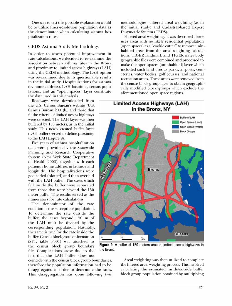
Roadways were downloaded from the U.S. Census Bureau’s website (U.S. Census Bureau 2001(b), and those that fit the criteria of limited access highways were selected. The LAH layer was then buffered by 150 meters, as in the initial study. This newly created buffer layer (LAH buffer) served to define proximity to the LAH (Figure 9).

Five years of asthma hospitalization data were provided by the Statewide Planning and Research Cooperative System (New York State Department of Health 2003), together with each patient’s home address in latitude and longitude. The hospitalizations were geo-coded (plotted) and then overlaid with the LAH buffer. The cases which fell inside the buffer were separated from those that were beyond the 150 meter buffer. The results served as the numerators for rate calculations.

The denominator of the rate equation is the susceptible population. To determine the rate outside the buffer, the cases beyond 150 m of the LAH must be divided by the corresponding population. Naturally, the same is true for the rate inside the buffer. Census block group information (SF1, table P001) was attached to the census block group boundary file. Complications arose due to the fact that the LAH buffer does not coincide with the census block group boundaries, therefore the population information had to be disaggregated in order to determine the rates. This disaggregation was done following two

methodologies—filtered areal weighting (as in the initial study) and Cadastral-based Expert Dasymetric System (CEDS).

Filtered areal weighting, as was described above, uses areas with no likely residential population (open spaces) as a “cookie cutter” to remove unin-habited areas from the areal weighting calcula-tions. TIGER landmark and TIGER water body geographic files were combined and processed to make the open spaces (uninhabited) layer which included such land uses as parks, airports, cem-eteries, water bodies, golf courses, and national recreation areas. These areas were removed from the census block group layer to obtain geographi-cally modified block groups which exclude the aforementioned open space regions.

Areal weighting was then utilized to complete the filtered areal weighting process. This involved calculating the estimated inside/outside buffer block group population obtained by multiplying

Figure 9. A buffer of 150 meters around limited-access highways in the Bronx.


the original census block group population by the ratio of the buffer area (inside or outside) and fil-tered block group area (excluding open spaces). It is important to note that this weighting technique makes the assumption that the population is uniformly distributed within each filtered census block group. The process can be written as follows:

POP_INFAW = POPBG * AREAIB / AREABG

POP_OUTFAW = POPBG * AREAOB / AREABG (7)

where:POP_INFAW = estimated population inside the

LAH buffer from filtered areal weighting;

POP_OUTFAW = estimated population outside the LAH buffer from filtered areal weighting;

POPBG = census block group population; AREAIB = filtered census block group

area inside the LAH buffer (open spaces excluded);

AREAOB = filtered census block group area outside the LAH buffer (open spaces excluded); and

AREABG = filtered census block group area (open spaces excluded).

The CEDS methodology, as described in detail elsewhere in this paper, was used to disag-gregate the census block group population to the tax-lot level. A combination of number of residential units and residential area was used as ancillary data to redistribute the population. Pop-ulations inside and outside the buffer were calculated by select-ing the tax lots whose centroids fall inside and outside the 150 m LAH buffers and summing the associated populations. With this method, population is not assumed to be homogeneous; instead, cadastral information regarding residential dwellings is used to redistribute the data preferentially. The equations can be written as follows:

POP_INCEDS = Σ LOTPOPi * M

POP_OUTCEDS = Σ LOTPOPi * |M-1| (8)

where:POP_INCEDS = estimated population inside the

LAH buffer from CEDS;

POP_OUTCEDS = estimated population outside the LAH buffer from CEDS;

LOTPOPi = CEDS-derived tax lot population for tax lot i; and

M = 1 if LOTi has its centroid within the LAH buffer, else it has a value of 0.

CEDS Asthma Study Results and DiscussionSince it can be difficult to visualize the difference in methodologies on small-scale maps (i.e., the entire Bronx), three block groups were selected in the South Bronx to illustrate the methods and respective results more explicitly. Filtered areal weighting and CEDS techniques were performed on the selected block groups containing a popu-lation of 2,166. Two sets of data were obtained for this area, which show a dramatic distinction between the methods even though they may not necessarily be representative of the entire Bronx. The filtered areal weighting resulted in an estimation of 1,017 people (~47 percent) of the three selected block groups residing within 150 meters of an LAH and 1,149 people (~53 percent) lived outside of the buffer. The CEDS

method estimated that only 57 people (~3 per-cent) were within the LAH buffer and 2,109 (~97 percent) were outside of the 150 meter threshold (see Figures 10 and 11). This some-what stark example demonstrates the utility of the CEDS methodology and the usefulness of

Figure 10. Population estimation inside and outside buffers, using filtered areal weighting versus CEDS Method, for three selected block groups, as shown in Figure 11.

Vol. 34, No. 2 97

having a more realistic understanding of popu-lation distribution.

The phenomenon that is apparent in the three-block group example above can also be seen in the entire Bronx. Between 1995 and 1999 (the study time frame) there was an average of 8,623 asthma hospitalizations in the Bronx per year. Inside the

Bronx-wide LAH buffer there were 950 hospital-izations per year, and outside the buffer there were 7,672 hospitalizations per year. Rates were calcu-lated by dividing the number of asthma hospitaliza-tions by the susceptible population, as follows:

RATEBX = CASESBX / POPBX

Figure 11. Visual representation of the comparison of filtered areal weighting and CEDS method.


RATEIN = CASESIN / POPIN

RATEOUT = CASESOUT / POPOUT (9)

where:RATE = rate of asthma hospitalization per year;CASES = five-year average asthma

hospitalization; POP = population; BX = Bronx; IN = inside the 150 m LAH buffer; and OUT = outside the 150 m LAH buffer.

Using Equation (9), the asthma hospitalization rate for the entire Bronx was approximately 6.53 per 1,000 people per year. The results with the filtered areal weighting methodology were some-what counterintuitive. Inside the buffer, the rate of susceptible populations was 6.20 per 1,000 people per year, whereas outside the buffer, the rate was 6.58 per 1,000 people per year, i.e., greater than the inside rate. If exposure to certain outdoor air pollution increases asthma hospitalizations, and close proximity to limited access highways increases exposure to this pollution, one would assume that

living in close proximity to an LAH would show an elevated rate of asthma hospitalizations when compared with those living beyond this threshold. The filtered areal weighting methodology, however, claims that the opposite is true. Although there are many other sources of outdoor air pollution in the Bronx, and also many other variables which may increase asthma hospitalization rates, the results were nonetheless unexpected.

When using the CEDS method, however, the results were quite different. Rates inside the buffer were found to be 7.03 per 1,000 people per year and outside the buffer 6.49 per 1,000 people per year (see Figure 12a). An examination of the stan-dardized incidence ratios (SR) by filtered areal weighting shows that residing within the LAH buffer is protective, with a 5 percent lower chance of being hospitalized for asthma. However when the CEDS-derived data are used as the denomi-nator, the SR shows a 7.5 percent higher chance for being hospitalized for asthma when residing within the LAH buffer (see Figure 12b). These CEDS-derived results, based on the more precise

Figure 12a. Estimated asthma hospitalization rates inside and outside buffers for the entire Bronx, with filtered areal weighting versus CEDS method.

Vol. 34, No. 2 99

location information of the population, seem to bolster the hypothesis that exposure to pollutants released from the limited access highways in the Bronx elevate asthma hospitalization rates.

The reason for this inconsistency in asthma rates is clearly a product of the difference in methodology for population estimation. The filtered areal weighting method estimates that 11.60 percent of the population resides within 150 meters of the LAH, whereas the CEDS method estimates only 10.25 percent of the population in the same area. With a smaller population (denominator), the rates, given equal number of hospitalizations (numerator), will be higher. The inverse is true for the results outside the buffer (88.40 percent and 89.75 percent for filtered areal weighting and CEDS, respectively).

Dasymetric Mapping—Where Do We Go From Here?

Based on the application of the CEDS methodol-ogy to New York City population data and given the case study example of asthma hospitalization rates in the Bronx, we have demonstrated that

the Cadastral-based Expert Dasymetric System can improve research and analyses that utilize population distribution information, while also creating more realistic models of real-world con-ditions. We are currently exploring techniques for modifying the CEDS methodology to esti-mate the spatial distribution of sub-populations, such as those characterized by race/ethnicity, age cohort, gender, or family structure. By employ-ing different ancillary data sets, socio-economic variables may also be mapped dasymetrically with the CEDS method.

We have established the usefulness of the CEDS method for any analyses employing population-based rates (such as public health and epidemiological research, crime mapping, and risk assessment), but the CEDS method is not limited to improving the development of rates alone. This method will be useful in many disparate fields and serve many purposes. For instance, one can improve emergency management operations and implementation by providing more precise information about actual positions of susceptible populations, thereby increas-ing the quality of functions such as evacuation route planning, optimal site selection for emergency shelter locations, and critical rescue and recovery

Figure 12b. Estimated asthma hospitalization rates inside and outside buffers for the entire Bronx, represented by standardized ratios, with filtered areal weighting versus CEDS method.


prioritization for first responders. Obviously, this can be extended to police operations, criminal justice, fire and ambulance services, utility provid-ers, and any other crucial public support systems dependant upon population information.

Additionally, the knowledge of accurate popula-tion distribution can be extremely valuable in the sphere of urban planning. The understanding of the locational characteristics of target populations would allow for more equitable resource alloca-tion in areas such as community infrastructure development, provision of open space and recre-ational opportunities, transportation access, and necessary environmental facilities.

As the morphology of cities becomes increasingly complex, the need continues to grow for immediate and well informed decision-making with regard to both catastrophic and everyday events. We anticipate that advances in dasymetric mapping, such as the CEDS method, will help us to “perfect the denominator” and better our understanding of the human urban project.

ACKNOWLEDGEMENTS

This research was partially supported by grant number 2 R25 ES01185-05 from the National Institute of Environmental Health Sciences of the National Institutes of Health. The National Oceanic and Atmospheric Administration’s Cooperative Remote Sensing Science and Technology Center (NOAA-CREST) also pro-vided critical support for this project under NOAA grant number NA17AE162. The state-ments contained within this paper are not the opinions of the funding agency or the U.S. government, but reflect the authors’ opinions. Thanks are also due to the member organiza-tions of the South Bronx Environmental Justice Partnership, who understood the relevance of this project to environmental health justice and gave their unstinting encouragement and assis-tance in the effort.

REFERENCES

Baudot, Y. 2001. A method for the geographical analysis of the population of fast-growing cities in the Third World. In: Donnay, J.-P., Barnsley, M., and Longley, P. (eds), Remote sensing and urban analysis. London, U.K.: Taylor and Francis. pp. 249-68.

Bhaduri, B., E. Bright, P. Coleman, and J. Dobson. 2002. LandScan: Locating people is what matters. GeoInformatics April/May: 34-35, 37.

Bielecka, E. 2005. A dasymetric population density map of Poland. In: Proceedings of the 22nd International Cartographic Conference, July 9-15, A Coruna, Spain.

Bracken, I., and D. Martin. 1989. The generation of spatial population distributions from Census centroid data. Environmental and Planning A, 21:537-43.

Cai, Q., B. Bhaduri, P. Coleman, G. Rushton, and E. Bright. 2006. Estimating small-area populations by age and sex using spatial interpolation and statistical inference methods. Transactions in GIS 10(4): 577-98.

Clarke, M., and J. A. Maantay. 2006. Optimizing recycling in all of New York City’s neighborhoods: Using GIS to develop the REAP index for improved Recycling Education, Awareness, and Participation. Resources, Conservation, and Recycling 46 (2): 128-48.

Dent, B.D. 1999. Cartography: Thematic map design. New York, New York: McGraw Hill.

Dorling, D., and D. Fairbairn. 1997. Mapping: Ways of representing the world. Prentice Hall, Upper Saddle River, New Jersey: Prentice Hall.

Eicher, C., and C. Brewer. 2001. Dasymetric mapping and areal interpolation: Implementation and evaluation. Cartography and Geographic Information Science 28:125-38.

ESRI (Environmental Systems Research Institute). 2005. ArcGIS 9.1. Redlands, California, USA.

Flowerdew, R., and M. Green. 1994. Areal interpolation and types of data. In: Fotheringham, A.S. and Rogerson, P.A., (eds), Spatial analysis and GIS. London, U.K.: Taylor and Francis. pp. 121-45.

Flowerdew, R., and M. Green. 1992. Developments in areal interpolation methods and GIS. Annals of Regional Science 26: 67-78.

Flowerdew, R., and M. Green. 1989. Statistical methods for inference between incompatible zonal systems. In: Goodchild, M.F., and S. Gopal (eds), Accuracy of spatial databases. London, U.K.: Taylor and Francis. pp. 239-48.

Flowerdew, R., M. Green, and E. Kehris. 1991. Using areal interpolation method in geographic information systems. Papers in Regional Science 70: 303-15.

Forster, B.C. 1985. An examination of some problems and solutions in monitoring urban areas from satellite platforms. International Journal of Remote Sensing 6(1): 139-51.

Goodchild, M., and N.S-N. Lam. 1980. Areal interpolation: A variant of the traditional spatial problem. Geo-Processing 1: 297-312.

Goodchild, M., L. Anselin, and U. Deichmann. 1993. A framework for the areal interpolation of socioeconomic data. Environment and Planning A 25: 383-97.

Gotway, C., and L. Young. 2002. Combining incompatible spatial data. Journal of the American Statistical Association 97: 632-48.

Gregory, I. N. 2000. An evaluation of the accuracy of the areal interpolation of data for the analysis of long-term change in England and Wales. In: Proceedings of the 5th International Conference on GeoComputation, University of Greenwich, United Kingdom, 23 - 25 August 2000.

Vol. 34, No. 2 101

Hall, S. 1994. Mapping the next millenium: The discovery of new geographies. New York, New York: Random House.

Herrmann, C., and A.R. Maroko. 2006. Crime pattern analysis: Exploring Bronx auto thefts using GIS. In: Maantay, J.A., and J. Ziegler, GIS for the Urban Environment. Redlands, California: ESRI Press.

Holloway, S.R., J. Schumacher, and R.L. Redmond. 1999. People and place: dasymetric mapping using Arc/Info. Pages 283-291 in S. Morain, ed. GIS Solutions in Natural Resource Management. OnWord Press, Santa Fe, New Mexico.

Holt, J. B., C. P. Lo, and T. W. Hodler. 2004. Dasymetric estimation of population density and areal interpolation of census data. Cartography and Geographic Information Science 31:103-21.

Koch, T. 2005. Cartographies of disease: Maps, mapping, and medicine. Redlands, California: ESRI Press.

Kyriakidis, P. 2004. A geostatistical framework for area to point spatial interpolation. Geographical Analysis 36(3):259-89.

Langford, M., D.J. Maguire, and D. Unwin. 1991. The areal interpolation problem: Estimating population using remote sensing in a GIS framework. In: Masser, I., and M. Blakemore (eds), Handling geographic information: Methodology and potential applications. London, U.K.: Longman.

Langford, M., and D. Unwin. 1994. Generating and mapping population density surfaces within a geographical information system. Cartographic Journal 31: 21-6.

Liu, X., K. Clarke, and M. Herold. 2006. Population density and image texture: A comparison study. Photogrammetric Engineering and Remote Sensing 72(2):187-96.

LotInfo, LLC. 2001. LotInfo. SpaceTrack, Inc. 304 Park Ave, 11th Floor New York, NY 10010.

Maantay, J.A., 2007/2005. Asthma and air pollution in the Bronx: Methodological and data considerations in using GIS for environmental justice and health research. Health and Place [Special Issue: Linking Environmental Justice, Population Health, and Geographical Information Science] 23: 32-56. (E-published, November 24, 2005).

Maantay, J.A. 2002. Industrial zoning changes in New York City and environmental justice: A case study in

“expulsive” zoning. Projections: the Planning Journal of Massachusetts Institute of Technology (MIT). (Special Issue: Planning for Environmental Justice). pp. 63-108.

Maantay, J.A. 2001. Zoning, equity, and public health. American Journal of Public Health 91(7):1033–41.

Maantay, J.A., and A. H. Strelnick. 2003. Mapping asthma hot spots: The geography of asthma and air pollution in the Bronx. Journal of Urban Health, Bulletin of the New York Academy of Medicine Vol. 80, Supplement 2, Oxford University Press.

Maroko, A.R., and J.A. Maantay. Residential racial segregation and health disparities in New York City: Mapping TB and AIDS in conjunction with

segregation indices. Unpublished research study, Urban GISc Lab, Lehman College.

Martin, D. 2006. An assessment of surface and zonal models of population. International Journal of Geographical Information Systems 10(8): 973-89.

Martin, D., M. Langford, and N.J. Tate. 2000. Refining population surface models: Experiments with Northern Ireland census data. Transactions in GIS 4(4): 343-60.

Mennis, J. 2003. Generating surface models of population using dasymetric mapping. The Professional Geographer 55(1): 31-42.

Mennis, J., and T. Hultgren. 2005. Dasymetric mapping for disaggregating coarse resolution population data. In: Proceedings of the 22nd Annual International Cartographic Conference, July 9-16, 2005, A Coruna, Spain.

Moon, Z.K., and F. L. Farmer. 2001. Population density surface: A new approach to an old problem. Society and Natural Resources 14: 39-49.

New York City Department of Health. 2003. Asthma facts, 2nd ed. New York, New York. [http://www.nyc.gov/html/doh/pdf/asthma/facts.pdf.]

New York State Department of Health, Statewide Planning and Research Cooperative System. 2003. Technical Documentation. Albany, New York.

Ong, P., and D. Houston. 2003. Draft Socioeconomic Report for 2003 Air Quality Management Plan. South Coast Air Quality Management District, Diamond Bar, California.

Openshaw, S. 1984. Ecological fallacies and the analysis of areal census data. Environmental and Planning A 16: 17-31.

Poulsen, E., and L.W. Kennedy. 2004. Using dasymetric mapping for spatially aggregated crime data. Journal of Quantitative Criminology 20(3): 243-62.

Reibel, M., and M.E. Bufalino. 2005. Street-weighted interpolation techniques for demographic count estimation in incompatible zone systems. Environmental and Planning A 37: 127-39.

Robinson, A.H. 1982. Early thematic mapping in the history of cartography. Chicago, Illinois: University of Chicago Press.

Scrope, G.P. 1833. Principles of Political Economy, Deduced from the Natural Laws of Social Welfare, and Applied to the Present State of Britain. London, U.K.: Longmans.

Sleeter, R. 2004. Dasymetric mapping techniques for the San Francisco Bay region, California. In: Urban and Regional Information Systems Association Annual Conference Proceedings, Reno, Nevada, November 7-10, 2004.

Slocum, T.A. 1999. Thematic cartography and visualization. Upper Saddle River, New Jersey: Prentice Hall.

Tobler, W. 1979. Smooth pycnophylactic interpolation for geographical regions. Journal of the American Statistical Association 74: 519-36.

United States Bureau of the Census. 2001(a). Census 2000 Summary File 1, New York State. Washington, D.C.


A message from the publisher of CaGIS

CaGIS onlineCartography and Geographic Information Science (CaGIS) has been published online since 2003, and soon, all CaGIS volumes published since 1974 will be available online. In order to access individual articles, you need to register for access.

members go to: http://www.ingentaconnect.com/content/acsm/cagis

Follow the information in the Page Help bar on the left to “Need to register? Sign up here.” Select the option for personal registration.

• Enter your information in the fields provided; and• Choose a username and password (username/password must be at least 5 characters).

Once you have entered all relevant information, please click on “Register.”You can then set up your “Personal Subscriptions” thus:

• Search for the journal title(s) you subscribe to; and• Enter in your publisher subscription number, check next to the journal title, and then press

“Add.”

You will then receive a confirmation message that your request has been received. An e-mail will then be sent out when access has been set up. Alternatively, go to: https://www.ingentaconnect.com/register/personal and follow instructions. You may need your MO member ID to successfully complete the registration.

Online CaGIS is provided to members of the Cartography and Geographic Information Society at no additional cost!! Members also have the option to opt for online only … mark your renewal forms accordingly, if you want to receive only the online version of the journal.

If you are not a member of CaGIS and wish to receive this great benefit, apply for membership at http://www.cartogis.org/membership.

We hope that you have a very pleasant experience browsing your online CaGIS. Should you require further help with registration or accessing CaGIS online, the Help Desk at http://www.ingentaconnect.com will be happy to provide further instructions.

CaGIS publisher www.cartogis.org

United States Bureau of the Census. 2001(b). TIGER Files. Geography Division, Cartographic Products Management Branch. Washington, D.C.

Weichselbaum, J., F. Petrini-Monteferri, M. Papathoma, W. Wagner, and N. Hackner. 2005. Sharpening census information in GIS to meet real-world conditions: The case for Earth observation. WIT Transactions on Ecology and the Environment, Sustainable Development and Planning II 1: 143-52.

Wright, J.K. 1936. A method of mapping densities of population with Cape Cod as an example. Geographical Review 26: 103-10.

Wu, S., X. Qiu, and L. Wang. 2005. Population estimation methods in GIS and remote sensing: A review. GIScience and Remote Sensing 42(1): 80-96.

Xie, Y. 1996. The overlaid network algorithms for areal interpolation problem. Computers, Environment, and Urban Systems 19: 287-306.

the cadastral-based expert dasymetric system - lehman college

Documents