lable at ScienceDirect

Quaternary Research 86 (2016) 271e286

Contents lists avai

Quaternary Research

journal homepage: http: / /www.journals .e lsevier .com/quaternary-research

The Carolina Sandhills: Quaternary eolian sand sheets and dunesalong the updip margin of the Atlantic Coastal Plain province,southeastern United States

Christopher S. Swezey a, *, Bradley A. Fitzwater b, G. Richard Whittecar b,Shannon A. Mahan c, Christopher P. Garrity d, Wilma B. Alem�an Gonz�alez a,Kerby M. Dobbs e

a U.S. Geological Survey, 12201 Sunrise Valley Drive, MS 926A, Reston, VA 20192, USAb Old Dominion University, Dept. of Ocean, Earth, and Atmospheric Sciences, Norfolk, VA 23529, USAc U.S. Geological Survey, Box 25046 Denver Federal Center, MS 974, Denver, CO 80225, USAd U.S. Geological Survey, 12201 Sunrise Valley Drive, MS 956, Reston, VA 20192, USAe Maser Consulting, 2000 Midlantic Drive, MT. Laurel, NJ 08054, USA

a r t i c l e i n f o

Article history:Received 8 March 2016Available online 20 October 2016

Keywords:EolianPinehurst FormationQuaternarySouth Carolina

* Corresponding author.E-mail address: cswezey@usgs.gov (C.S. Swezey).

http://dx.doi.org/10.1016/j.yqres.2016.08.0070033-5894/Published by Elsevier Inc. on behalf of Un

a b s t r a c t

The Carolina Sandhills is a physiographic region of the Atlantic Coastal Plain province in the southeasternUnited States. In Chesterfield County (South Carolina), the surficial sand of this region is the PinehurstFormation, which is interpreted as eolian sand derived from the underlying Cretaceous MiddendorfFormation. This sand has yielded three clusters of optically stimulated luminescence ages: (1) 75 to 37thousand years ago (ka), coincident with growth of the Laurentide Ice Sheet; (2) 28 to 18 ka, coincidentwith the last glacial maximum (LGM); and (3) 12 to 6 ka, mostly coincident with the Younger Dryasthrough final collapse of the Laurentide Ice Sheet. Relict dune morphologies are consistent with windsfrom the west or northwest, coincident with modern and inferred LGM January wind directions. Sandsheets are more common than dunes because of effects of coarse grain size (mean range: 0.35e0.59 mm)and vegetation. The coarse grain size would have required LGM wind velocities of at least 4e6 m/sec,accounting for effects of colder air temperatures on eolian sand transport. The eolian interpretation ofthe Carolina Sandhills is consistent with other evidence for eolian activity in the southeastern UnitedStates during the last glaciation.

Published by Elsevier Inc. on behalf of University of Washington.

Introduction

The Carolina Sandhills is a 15e60 kmwide physiographic regionthat extends from the western border of Georgia (GA) across SouthCarolina (SC) to central North Carolina (NC) along the updip (northand west) margin of the Atlantic Coastal Plain province in thesoutheastern United States (Fig. 1). This region is characterized byabundant unconsolidated sand that has been recognized for a longtime (e.g., McGee, 1890, 1891; Holmes, 1893), although previousstudies of this region are surprisingly few and previous in-terpretations of the sand have been quite speculative. Cooke (1936),for example, suggested that eolian processes played a role in

iversity of Washington.

shaping the topography of the area (which he called the “CongareeSand Hills”), and he noted that the area of the sand hills corre-sponds to the area where the Cretaceous Tuscaloosa Formation[Middendorf Formation] is exposed. Other previous studies inSouth Carolina have referred to the sand hills as being of post-Eocene age, and speculations on depositional environment haveranged from eolian to fluvial to marine (Johnson,1961; Otwell et al.,1966; Ridgeway et al., 1966; Kite, 1987; Nystrom and Kite, 1988).Nystrom et al. (1991) stated that the sand hills are widespreaddeposits of sand dispersed discontinuously across the upper coastalplain from northern Aiken County (SC) northeastward to the SC-NCborder, and that these deposits are the southwestern continuationof the Pinehurst Formation of North Carolina, as named by Conley(1962) and redefined by Bartlett (1967). Nystrom et al. (1991)interpreted the sand as eolian dunes, sand sheets, and interdunedeposits of LateMiocene age. However, a subsequent detailed study

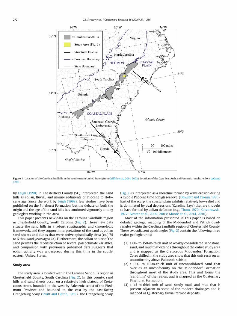
Figure 1. Location of the Carolina Sandhills in the southeastern United States (from Griffith et al., 2001, 2002). Locations of the Cape Fear Arch and Peninsular Arch are from LeGrand(1961).

C.S. Swezey et al. / Quaternary Research 86 (2016) 271e286272

by Leigh (1998) in Chesterfield County (SC) interpreted the sandhills as eolian, fluvial, and marine sediments of Pliocene to Holo-cene age. Since the work by Leigh (1998), few studies have beenpublished on the Pinehurst Formation, but the debate on both theorigin and the age of the sand hills has continued vigorously amonggeologists working in the area.

This paper presents new data on the Carolina Sandhills regionin Chesterfield County, South Carolina (Fig. 2). These new datasituate the sand hills in a robust stratigraphic and chronologicframework, and they support interpretations of the sand as eoliansand sheets and dunes that were active episodically circa (ca.) 75to 6 thousand years ago (ka). Furthermore, the eolian nature of thesand permits the reconstruction of several paleoclimate variables,and comparison with previously published data suggests thateolian activity was widespread during this time in the south-eastern United States.

Study area

The study area is located within the Carolina Sandhills region inChesterfield County, South Carolina (Fig. 2). In this county, sandhills and sand sheets occur on a relatively high plateau of Creta-ceous strata, bounded to the west by Paleozoic schist of the Pied-mont Province and bounded to the east by the east-facingOrangeburg Scarp (Swift and Heron, 1969). The Orangeburg Scarp

(Fig. 2) is interpreted as a shoreline formed by wave erosion duringamiddle Pliocene time of high sea level (Dowsett and Cronin,1990).East of the scarp, the coastal plain exhibits relatively low-relief andis dominated by oval depressions (Carolina Bays) that are thoughtto have formed by eolian deflation (e.g., Thom, 1970; Kaczorowski,1977; Ivester et al., 2002, 2003; Moore et al., 2014, 2016).

Most of the information presented in this paper is based ondetailed geologic mapping of the Middendorf and Patrick quad-rangles within the Carolina Sandhills region of Chesterfield County.These two adjacent quadrangles (Fig. 2) contain the following threemajor geologic units:

(1) a 60- to 150-m-thick unit of weakly consolidated sandstone,sand, and mud that extends throughout the entire study areaand is mapped as the Cretaceous Middendorf Formation.Cores drilled in the study area show that this unit rests on anunconformity above Paleozoic schist;

(2) a 0.3- to 10-m-thick unit of unconsolidated sand thatoverlies an unconformity on the Middendorf Formationthroughout most of the study area. This unit forms the“sandhills” of the region, and is mapped as the QuaternaryPinehurst Formation;

(3) a <3-m-thick unit of sand, sandy mud, and mud that ispresent adjacent to some of the modern drainages and ismapped as Quaternary fluvial terrace deposits.

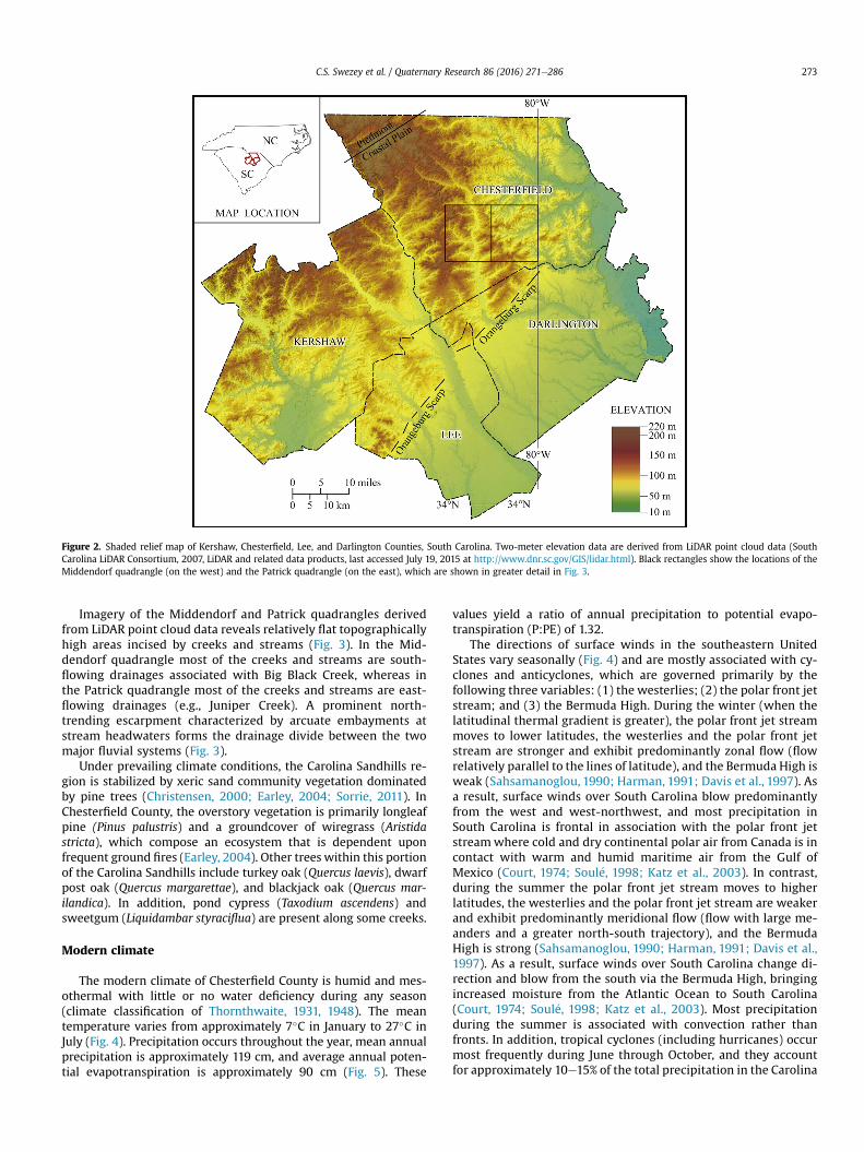
Figure 2. Shaded relief map of Kershaw, Chesterfield, Lee, and Darlington Counties, South Carolina. Two-meter elevation data are derived from LiDAR point cloud data (SouthCarolina LiDAR Consortium, 2007, LiDAR and related data products, last accessed July 19, 2015 at http://www.dnr.sc.gov/GIS/lidar.html). Black rectangles show the locations of theMiddendorf quadrangle (on the west) and the Patrick quadrangle (on the east), which are shown in greater detail in Fig. 3.

C.S. Swezey et al. / Quaternary Research 86 (2016) 271e286 273

Imagery of the Middendorf and Patrick quadrangles derivedfrom LiDAR point cloud data reveals relatively flat topographicallyhigh areas incised by creeks and streams (Fig. 3). In the Mid-dendorf quadrangle most of the creeks and streams are south-flowing drainages associated with Big Black Creek, whereas inthe Patrick quadrangle most of the creeks and streams are east-flowing drainages (e.g., Juniper Creek). A prominent north-trending escarpment characterized by arcuate embayments atstream headwaters forms the drainage divide between the twomajor fluvial systems (Fig. 3).

Under prevailing climate conditions, the Carolina Sandhills re-gion is stabilized by xeric sand community vegetation dominatedby pine trees (Christensen, 2000; Earley, 2004; Sorrie, 2011). InChesterfield County, the overstory vegetation is primarily longleafpine (Pinus palustris) and a groundcover of wiregrass (Aristidastricta), which compose an ecosystem that is dependent uponfrequent ground fires (Earley, 2004). Other trees within this portionof the Carolina Sandhills include turkey oak (Quercus laevis), dwarfpost oak (Quercus margarettae), and blackjack oak (Quercus mar-ilandica). In addition, pond cypress (Taxodium ascendens) andsweetgum (Liquidambar styraciflua) are present along some creeks.

Modern climate

The modern climate of Chesterfield County is humid and mes-othermal with little or no water deficiency during any season(climate classification of Thornthwaite, 1931, 1948). The meantemperature varies from approximately 7�C in January to 27�C inJuly (Fig. 4). Precipitation occurs throughout the year, mean annualprecipitation is approximately 119 cm, and average annual poten-tial evapotranspiration is approximately 90 cm (Fig. 5). These

values yield a ratio of annual precipitation to potential evapo-transpiration (P:PE) of 1.32.

The directions of surface winds in the southeastern UnitedStates vary seasonally (Fig. 4) and are mostly associated with cy-clones and anticyclones, which are governed primarily by thefollowing three variables: (1) the westerlies; (2) the polar front jetstream; and (3) the Bermuda High. During the winter (when thelatitudinal thermal gradient is greater), the polar front jet streammoves to lower latitudes, the westerlies and the polar front jetstream are stronger and exhibit predominantly zonal flow (flowrelatively parallel to the lines of latitude), and the Bermuda High isweak (Sahsamanoglou, 1990; Harman, 1991; Davis et al., 1997). Asa result, surface winds over South Carolina blow predominantlyfrom the west and west-northwest, and most precipitation inSouth Carolina is frontal in association with the polar front jetstreamwhere cold and dry continental polar air from Canada is incontact with warm and humid maritime air from the Gulf ofMexico (Court, 1974; Soul�e, 1998; Katz et al., 2003). In contrast,during the summer the polar front jet stream moves to higherlatitudes, the westerlies and the polar front jet stream are weakerand exhibit predominantly meridional flow (flow with large me-anders and a greater north-south trajectory), and the BermudaHigh is strong (Sahsamanoglou, 1990; Harman, 1991; Davis et al.,1997). As a result, surface winds over South Carolina change di-rection and blow from the south via the Bermuda High, bringingincreased moisture from the Atlantic Ocean to South Carolina(Court, 1974; Soul�e, 1998; Katz et al., 2003). Most precipitationduring the summer is associated with convection rather thanfronts. In addition, tropical cyclones (including hurricanes) occurmost frequently during June through October, and they accountfor approximately 10e15% of the total precipitation in the Carolina

Figure 3. Shaded relief map of the Middendorf and Patrick quadrangles, Chesterfield County, South Carolina. Two-meter elevation data are derived from LiDAR point cloud data(South Carolina LiDAR Consortium, 2007, LiDAR and related data products, last accessed July 19, 2015 at http://www.dnr.sc.gov/GIS/lidar.html). White circles with numbers denoteOSL sites, and white squares denote small towns.

Figure 4. Data from January (left image) and July (right image) of modern mean temperature in degrees Celsius (Webb et al., 1993), and mean resultant velocity and direction ofsurface winds based on hourly observations from 1951 through 1960 (data from Baldwin, 1975). The wind velocity in meters per second (m/s) is written inside each circle, and is alsodenoted by the length of the gray arrows. The mean resultant wind is the vectorial average of all wind velocities and wind directions at a given place during the specified months for1951 to 1960.

C.S. Swezey et al. / Quaternary Research 86 (2016) 271e286274

Figure 5. Mean annual precipitation in centimeters (Webb et al., 1993) and mean annual evapotranspiration in centimeters (Thornthwaite, 1948).

C.S. Swezey et al. / Quaternary Research 86 (2016) 271e286 275

portion of the coastal plain (Court, 1974; Knight and Davis, 2007).During some summers, however, the western sector of theBermuda High moves westward of its mean position to an inlandlocation over the southeastern United States, and moisture fluxfrom the Gulf of Mexico to the southeastern United States isreduced (Stahle and Cleaveland, 1992).

The mean resultant velocity of surface winds in South Carolinais <3 m/sec during any given month (Fig. 4), but there is somevariability (“gustiness”) around the mean. Detailed hourly datafrom the Metropolitan Airport at the city of Columbia (CarolinaSandhills region, approximately 100 km southwest of the Mid-dendorf quadrangle) indicate that wind velocities of 6 m/sec orgreater occurred approximately 8% of the time per whole yearduring the interval of 1981e2010 (www.ncdc.noaa.gov; accessed 18August 2016). Using a 6 m/sec threshold wind velocity for eoliansand mobilization, the 1981e2010 data yield a drift potential of 75vector units (VU) and a resultant drift direction for eolian sedimentof 97� (slightly south of east). For reference, a drift potential of 75VU is in the “low-energy wind environment” category of Frybergerand Dean (1979).

Methods

Sediment grain sizes were described using terminology ofWentworth (1922) and Folk (1954, 1980). Selected samples weresubjected to size analysis using a Malvern Mastersizer 2000 laserdiffractometer (Fitzwater, 2016). Other samples were subjected tosieving analysis using mesh sizes at 0.5 phi (f) increments, andsieving times of at least 15 min per sample (following Folk andWard, 1957; Folk, 1966). For sieved samples, sediment sortingvalues were calculated from cumulative percent curves using thesorting formula of Folk and Ward (1957), and sediment texturalmaturity was described using terminology of Folk (1951, 1954,1956). A binocular microscope was used to determine both

sediment grain shape (using sphericity and roundness terminologyof Powers, 1953) and sediment grain composition. The determi-nation of sediment composition was done visually via pointcounting (following procedures of van der Plas and Tobi, 1965; Folket al., 1970; Folk, 1980).

Ground-penetrating radar (GPR) data were collected with aGeophysical Survey Systems, Inc. (GSSI) towed-array data acquisi-tion system using a Subsurface Interface Radar (SIR-3000) and 200megahertz (MHz) antenna outfitted with an integrated surveywheel that was calibrated in the field. Post-processing of GPR datawas conducted using RADAN (version 7) processing software.Specific GPR setup parameters and post-processing filter con-straints are described in Fitzwater (2016).

The ages of some sediment samples were determined usingoptically stimulated luminescence (OSL) techniques at the U.S.Geological Survey (USGS) luminescence laboratory in Denver, Col-orado (Tables 1 and 2). Samples were collected in 0.8-m-longopaque polyvinyl chloride (PVC) tubes that were hammered intothe sediment, in most instances at the base of pits dug into sandhills and terraces. The tubes were then extracted and capped toprevent light exposure. Following standard laboratory procedures(Wintle and Murray, 2006; Mahan et al., 2007), the samples weretreated with acids to remove carbonate and organic matter, andthen sieved to extract fine-grained sand (250e180 mm). Quartzsand was separated from other grains by heavy liquid immersion,and quartz grains were etched by hydrofluoric acid to remove theoutermost layer. The purified quartz samples were analyzed usingthe single-aliquot regeneration technique (Murray and Wintle,2000, 2003), and a minimum of 20 aliquots were measured foreach sample. Dose response tests, preheat plateau tests, and ther-mal transfer tests were performed to ensure that the sediment wasresponsive to optical techniques and that proper preheat temper-atures were used in producing the equivalent dose (DE) values. TheDE values were determined by the single-aliquot regenerative

Table 1Optically stimulated luminescence (OSL) data from sand of the Pinehurst Formation, Chesterfield County, South Carolina. CDA (Gy/ka) ¼ Cosmic Dose Additions (grays perthousand years) as calculated using the methods of Prescott and Hutton (1994); DEPTH (cm) ¼ sample depth (centimeters below surface); DR (Gy/ka) ¼ total dose rate (graysper thousand years) with cosmic dose additions (grays per thousand years) as calculated using the methods of Prescott and Hutton (1994); ELV (m) ¼ sample site elevation(meters above sea level); K (%) ¼ potassium content (percentage); LAT ¼ latitude; LONG ¼ longitude; SITE # (Fig. 3) ¼ OSL site number shown in Fig. 3; Th (ppm) ¼ thoriumcontent (parts per million); U (ppm) ¼ uranium content (parts per million); USGS ID ¼ U.S. Geological Survey OSL laboratory sample identification code; WATER (%) ¼ fieldmoisture (complete sample saturation percentage in parentheses); YEAR ¼ Year during which sample age was determined.

USGSID

YEAR SITE #(Fig. 3)

LAT (North) LONG (West) ELV (m) DPTH(cm)

WATER(%)

K (%) U (ppm) Th (ppm) CDA(Gy/ka)

DR (Gy/ka)

1585 2013 3 34.56355 �80.13365 113 42e47 2 (22) 0.24 ± 0.04 1.57 ± 0.21 5.75 ± 0.52 0.20 ± 0.02 1.10 ± 0.081586 2013 3 34.56355 �80.13365 113 65e70 2 (16) 0.23 ± 0.04 1.51 ± 0.20 6.20 ± 0.56 0.19 ± 0.01 1.14 ± 0.081588 2013 5 34.58355 �80.10430 125 42 5 (19) 0.24 ± 0.04 1.07 ± 0.24 3.82 ± 0.35 0.20 ± 0.02 0.89 ± 0.391589 2013 5 34.58355 �80.10430 125 85 3 (22) 0.25 ± 0.02 1.70 ± 0.11 6.55 ± 0.26 0.19 ± 0.01 2.31 ± 0.871642 2013 4 34.55686 �80.12839 119 200 4 (27) 0.21 ± 0.04 1.05 ± 0.18 6.77 ± 0.37 0.16 ± 0.01 0.96 ± 0.051643 2013 4 34.55686 �80.12839 119 60 7 (28) 0.24 ± 0.04 1.80 ± 0.23 8.52 ± 0.47 0.19 ± 0.01 1.27 ± 0.061715 2014 6 34.62072 �80.05958 76 210 6 (28) 0.22 ± 0.04 1.88 ± 0.24 10.5 ± 0.31 0.16 ± 0.01 1.35 ± 0.041716 2014 6 34.62072 �80.05958 76 250 3 (26) 0.12 ± 0.06 1.33 ± 0.33 5.36 ± 0.43 0.15 ± 0.01 0.85 ± 0.071717 2014 6 34.62072 �80.05958 76 250 4 (25) 0.17 ± 0.04 1.28 ± 0.28 6.07 ± 0.59 0.15 ± 0.01 0.93 ± 0.081718 2014 2 34.52557 �80.22427 122 40 6 (30) 0.35 ± 0.03 0.84 ± 0.21 3.02 ± 0.53 0.21 ± 0.02 0.83 ± 0.101719 2014 2 34.52557 �80.22427 122 145 6 (25) 0.14 ± 0.04 1.04 ± 0.23 2.16 ± 0.47 0.17 ± 0.01 0.63 ± 0.101720 2014 1 34.62237 �80.23235 125 90 9 (30) 0.25 ± 0.05 1.26 ± 0.21 5.90 ± 0.41 0.19 ± 0.02 0.99 ± 0.051721 2014 1 34.62237 �80.23235 125 160 7 (28) 0.40 ± 0.06 2.67 ± 0.27 10.2 ± 0.68 0.17 ± 0.01 1.65 ± 0.091722 2014 1 34.62237 �80.23235 125 210 10 (25) 0.43 ± 0.04 2.67 ± 0.28 10.60 ± 0.48 0.16 ± 0.01 1.72 ± 0.07

Table 2Optically stimulated luminescence (OSL) equivalent dose data and ages from sand of the Pinehurst Formation, Chesterfield County, South Carolina. Preferred ages (the agesestimated to be the most accurate) are shown in bold (see text for explanation). AGE (ka) MAM ¼ age in thousands of years (ka) ago using the OSL Minimum Age Model-3 forequivalent dose (DE) determinations; AGE (ka) Mean ¼ age in thousands of years (ka) ago using the mean OSL value for equivalent dose (DE) determinations; AGE (ka)Weighted ¼ age in thousands of years (ka) ago using the weighted mean OSL value for equivalent dose (DE) determinations. The ages presented in this table are reported inyears before the date of age determination, and are presented with a one-sigma standard deviation of the age uncertainty; DE (Gy) MAM ¼ equivalent dose (grays) using theMinimum Age Model-3 for DE determinations; DE (Gy) Mean ¼ equivalent dose (grays) using the mean OSL value for DE determinations (average of all DE with no filter ormodel); DE (Gy)Weighted¼ equivalent dose (grays) using theweightedmean OSL value for DE determinations; disp. (%)¼ dispersion (percentage) calculated as the average ofthe equivalent dose divided by the standard deviation of the equivalent dose; (n) DE¼ number of replicated equivalent dose estimates used to calculate themean value (total inparentheses denotes the total number of measurements of subsamples or aliquots, including failed runs with unusable data); SITE # (Fig. 3)¼ OSL site number shown in Fig. 3;USGS ID ¼ U.S. Geological Survey OSL laboratory sample identification code.

USGS ID SITE # (Fig. 3) DE (Gy) MAM DE (Gy) Weighted DE (Gy) Mean (n) DE Disp. (%) Age (ka) MAM Age (ka) Weighted Age (ka) Mean

1585 3 11.20 ± 0.45 12.40 ± 0.58 11.90 ± 0.70 12 (25) 26 10.16 ± 0.84 11.27 ± 0.98 10.82 ± 1.021586 3 27.50 ± 1.49 12.40 ± 1.15 29.10 ± 1.31 8 (30) 32 24.09 ± 2.20 24.12 ± 2.05 25.58 ± 2.221588 5 8.08 ± 0.33 8.36 ± 0.39 8.54 ± 0.49 24 (28) 11 9.08 ± 0.80 9.40 ± 0.82 9.60 ± 0.891589 5 22.60 ± 0.95 23.10 ± 0.87 26.60 ± 1.12 14 (24) 28 19.32 ± 1.63 19.65 ± 1.61 22.74 ± 1.911642 4 44.40 ± 1.91 44.20 ± 1.14 44.90 ± 3.04 9 (25) 40 46.29 ± 3.13 46.04 ± 2.67 46.77 ± 4.001643 4 32.90 ± 2.47 32.90 ± 2.47 33.60 ± 1.63 4 (17) 38 25.50 ± 2.30 26.46 ± 1.80 25.94 ± 2.301715 6 53.70 ± 3.20 63.80 ± 3.19 69.20 ± 3.18 15 (24) 31 39.80 ± 2.67 47.30 ± 2.78 51.30 ± 2.851716 6 53.20 ± 2.39 59.20 ± 1.36 57.00 ± 1.31 19 (24) 24 62.60 ± 5.64 69.60 ± 5.65 67.10 ± 5.461717 6 49.90 ± 2.25 44.00 ± 1.23 52.20 ± 1.30 18 (24) 41 53.70 ± 5.11 47.30 ± 4.19 56.10 ± 4.901718 2 5.78 ± 0.22 6.42 ± 0.38 7.33 ± 0.63 16 (20) 33 6.96 ± 0.91 7.73 ± 0.93 8.83 ± 1.331719 2 30.20 ± 1.45 30.80 ± 1.45 29.80 ± 1.62 21 (24) 20 47.90 ± 7.59 48.90 ± 7.73 47.30 ± 7.591720 1 36.50 ± 2.23 49.30 ± 2.22 52.40 ± 2.36 16 (20) 23 36.90 ± 3.16 49.80 ± 3.74 53.00 ± 3.891721 1 13.80 ± 0.65 15.20 ± 0.58 16.60 ± 0.75 18 (20) 21 8.41 ± 0.60 9.22 ± 0.61 10.10 ± 0.711722 1 18.80 ± 0.81 18.20 ± 0.82 19.00 ± 0.82 18 (24) 31 10.90 ± 0.64 10.60 ± 0.63 11.00 ± 0.64

C.S. Swezey et al. / Quaternary Research 86 (2016) 271e286276

(SAR) dose protocol (Murray andWintle, 2000; Wintle and Murray,2006).

The OSL ages were determined using an exponential and linearfit on the DE data, and the ages are reported in years before themeasured date with a one-sigma standard deviation of the ageuncertainty (Tables 1 and 2). Determination of DE values was madeusing the Minimum Age Model-3 (Galbraith and Laslett, 1993;Galbraith et al., 1999), the weighted mean (similar to the CentralAge Model of Galbraith et al., 1999), and themean (average of all DEvalues with no filter or model). All of the DE determinations and theresultant ages are shown in Table 2.

The dosimetry samples were taken from the tube OSL samples,and thus the dosimetry or dose rate (DR) data were measuredfrom the same sediment as each OSL sample. This sediment wasdried, homogenized by disaggregation, weighed, sealed in plan-chets (techniques modified from Murray et al., 1987), and placedin a gamma-ray spectrometer for determination of elemental

concentration of potassium (K), uranium (U), and thorium (Th).Field moisture (water content) was measured from the sedimentat the center of each tube in which the sample was collected.Saturation moisture was determined by putting dry sediment in atube, weighing the tube, filling the tube with water, centrifugingthe tube (to simulate compaction), and then draining the waterout of the tube and reweighing the sediment. The saturationmoisture content is the difference between this new weight andthe initial dry sediment weight.

Description of the Carolina Sandhills in the Middendorf andPatrick quadrangles

In the Middendorf and Patrick quadrangles, most of the land-scape is covered by amantle of unconsolidated sand that is mappedas the Pinehurst Formation. At many locations, the unconsolidatedsand is <2 m thick and forms a sand sheet of low relief. In areas of

Figure 7. Outcrop of Cretaceous Middendorf Formation, capped by unconformity,which is overlain by Quaternary Pinehurst Formation with OSL ages obtained using theMinimum Age Model-3 (modified from Swezey et al., 2016). Shovel and hoe provide asense of scale. This location is OSL site #4 (Tables 1 and 2). Location of outcrop isshown in Fig. 3. Similar details about the other OSL sites are available in Swezey et al.(2016).

C.S. Swezey et al. / Quaternary Research 86 (2016) 271e286 277

higher elevation, however, the unconsolidated sand can be up to10 m thick and forms subdued hills of up to 6 m relief with steepersides on the east and southeast (Fig. 6).

The unconsolidated sand (Pinehurst Formation) rests on anunconformity above a unit of sandstone, muddy sandstone tomuddy sand, andmud that is mapped collectively as the CretaceousMiddendorf Formation (Fig. 7). There is considerable relief on thisunconformity (up to 5m in places). Most outcrops of the Cretaceousstrata consist of grayish red (5R 4/2) to dark yellowish orange (10YR6/6) medium to coarse sandstone or sand (color nomenclature fromGoddard et al., 1963). At many locations, the Cretaceous strataimmediately beneath the unconformity display pedogenicmottling, and primary sedimentary structures are not obvious.Sieving analyses of individual samples of Cretaceous sand revealedthat the most frequently occurring grain size ranges from mediumsand (lower) to coarse sand (lower), and the most frequentlyoccurring sorting values (sf) range from 1.01 to 1.80 (poorly sor-ted). The sand-size grains consist mostly of quartz (99%) with 1%mica and opaque minerals. Most of the quartz grains of mediumsand size and coarser are subrounded to subangular, ranging fromhigh sphericity to low sphericity.

The unconsolidated sediment (Pinehurst Formation) above theCretaceous strata consists of grayish orange (10 YR 7/4) sand. Visualinspection of samples in the field showed that most of the sedimentis medium sand (upper) to coarse sand (lower). Sieving analysesrevealed that most samples have grain sizes ranging from fine(lower) sand (2.75 f, or 0.149 mm) to coarse (lower) sand (0.75 f,or 0.59 mm), and the most frequently occurring grain size of indi-vidual samples ranges frommedium (upper) to coarse (lower) sand(1.5e0.74 f, or 0.35e0.59 mm). Sorting values (sf) vary from 0.76to 1.65 (moderately sorted to poorly sorted). The sand-size grainsconsist predominantly of quartz (99%) with 1% mica and opaqueminerals. Most of the quartz grains of medium sand size andcoarser are subrounded to subangular, ranging from high sphericityto low sphericity. Textural maturity of the samples ranges fromimmature to submature.

Exposures of the unconsolidated sand (Pinehurst Formation)do not display primary sedimentary structures, although somestructures are visible in GPR data. For example, several GPR tra-verses across sand hills revealed 2e5-m thick sets of southeast-dipping cross-bedding at depths below 2 m (Fig. 8). Most expo-sures display evidence of bioturbation by vegetation (plant roots),

Figure 6. Shaded relief map showing details of “sandhill” morphology in the Mid-dendorf quadrangle, Chesterfield County, South Carolina. Two-meter elevation data arederived from LiDAR point cloud data (South Carolina LiDAR Consortium, 2007, LiDARand related data products, last accessed July 19, 2015 at http://www.dnr.sc.gov/GIS/lidar.html). Location of image is shown in Fig. 3.

and pedogenic features such as soil lamellae and modest argillichorizons. Soil types range from deeply weathered plinthitic ulti-sols to argillic ultisols to sandy entisols, and a few exposuresreveal a buried argillic Bt horizon. In the U.S. Department ofAgriculture soil survey of Chesterfield County (Morton, 1995),most of the area covered by the Pinehurst Formation is mapped asAlpin sand or Candor sand.

The OSL ages provide an absolute chronology for the PinehurstFormation. Samples from 6 sites yielded OSL ages ranging from ca.75 to 6 ka ago (Table 2; Fig. 9). One of these sites is shown inFigure 7, and additional details of these sites are given in Swezeyet al. (2016). Using a one-sigma standard deviation of the age un-certainty, one group of OSL ages ranges from ca. 75 to 37 ka, anothergroup of OSL ages ranges from ca. 28 to 18 ka, and a third group ofOSL ages ranges from ca. 12 to 6 ka.

Reliability of OSL data

For all OSL samples, the DR results were relatively homogenous(Table 1) and thus several potential problems such as OSL signalvariation or disequilibrium in the UeTh decay chain were notconsidered to be significant impediments to age determination.Some DE recovery tests had less scatter than the natural tests,indicating that some grains in the natural test carried largerluminescence signals. Such larger luminescence signals arethought to have been caused by in-situ dose hot-spots (concen-trations of heavy minerals or minerals with large K or U contents)that accumulated during sediment deposition. The larger lumi-nescence signals are not thought to have been caused by partialbleaching (non-zeroing) because: (1) the associated skew andscatter of DE were not indicative of partial bleaching (i.e., therewere only a few outliers rather than a uniform skew of progres-sively larger DE); (2) the DR results were low with observedscattered grains of apatite, potassium feldspar, and zircon; and (3)the dispersion in the results ranged from 11 to 41% (average ~26%).Thus, the most probable cause of the observed patterns of scatterin the DE values is that a few grains of quartz were subjected toincreased local radiation by proximity to feldspar or heavy min-eral grains.

Figure 8. Ground-penetrating radar (GPR) traverse over a sand hill in the Patrick quadrangle, Chesterfield County, South Carolina. Traverse location is shown in Fig. 3.

C.S. Swezey et al. / Quaternary Research 86 (2016) 271e286278

For many of the samples, the effects of bioturbation on the OSLages are thought to be negligible because of the absence of thefollowing features that are typically associated with bioturbation(e.g., Bateman et al., 2007a,b): (1) high dispersion values (e.g.,consistently >25%); (2) apparently zero-dose grains decliningwith depth from the surface; (3) significant differences betweensingle grains and single aliquots; and (4) greatly skewed multi-modal DE distributions. Some of the OSL samples, however, haverelatively high dispersion values (26e41%), which may indicatethat some local dose heterogeneity, sediment mixing, or bio-turbation has occurred. In these instances, any potential effects ofpossible bioturbation are not thought to be very great, possiblybecause bioturbation in the area is caused primarily by plant rootsrather than by animal activity that would be more likely to moveburied grains to the surface. Three samples from OSL site #6(USGS1715, -1716, -1717), for example, have significant differencesin dispersion values (24%, 31%, and 41%), but relatively similar OSLages. The similarity of the ages suggests that bioturbation may notbe a significant problem, or that bioturbation occurred onlywithin discrete beds. Two samples from OSL site #4 (USGS1642,-1643) also have higher dispersion values (38%, 40%), and it ispossible that these samples have been subjected to bioturbation,and thus the ages should be considered to be minimum ages ofeolian sediment mobilization. Nevertheless, the ages of these twosamples are consistent with the ages of other samples with lowerdispersion values. Two samples from OSL site #2 (USGS1718,-1719) have very different dispersion values (20%, 33%), and thesample with the larger dispersion value yielded a very young ageof ca. 7 ka. It is possible that this sample has been subjected tobioturbation, and thus the age should be considered to be aminimum age of eolian sediment mobilization. The OSL age of thissample, however, is similar to the age of sample USGS1588 fromOSL site #5, which had a dispersion value of only 11%, and thus theage of the sample with the 33% dispersion value (USGS1718) maybe reliable.

Table 2 shows separate columns with OSL age estimates ac-cording to various statistical models (Minimum Age Model-3,Weighted, Mean). In these columns, the preferred ages (thoseestimated to be the most accurate) are shown in bold. Thesepreferred ages were chosen as follows: If the dispersion is <25% (asdetermined by the R program radial plot, following Galbraith andRoberts, 2012), then the preferred age is that obtained by theweighted mean. If the dispersion is� 25%, then the preferred age isthat obtained by the Minimum Age Model-3. This choice of statis-tical models for the equivalent dose and the resulting ages followsthe recommendations of Galbraith and Roberts (2012) andReimann et al. (2012), although these authors used a dispersioncutoff value of 20%. For the Carolina Sandhills samples, however, a20% cutoff value was considered to be too restrictive and a 25%cutoff value was used instead because of the possibility of grains

having been mixed in the initial deposit via post-depositional dis-turbances (as discussed by Galbriath et al., 2012).

Interpretation of depositional environments

The unconsolidated sand (Pinehurst Formation) of the CarolinaSandhills is interpreted as eolian sand sheets and dunes derivedfrom the underlying Cretaceous sand, mobilized repeatedly duringconditions of colder temperatures and reduced vegetation cover,and then subsequently degraded and stabilized by pedogenesis andvegetation. As outlined below, the eolian interpretation of thePinehurst Formation is derived from an assemblage of thefollowing five characteristics: (1) sandhill location; (2) sandhillmorphology and primary sedimentary structures; (3) OSL ages; (4)grain-size data; and (5) bioturbation and pedogenic features. Anyone of these characteristics alone is not necessarily diagnostic of aneolian depositional environment, but the total assemblage of thesecharacteristics, as well as the overall setting and relations withunderlying strata, suggest that an eolian interpretation is mostlikely.

Sandhill location

The location of the Pinehurst Formation places some constraintson possible sediment sources and rules out some depositional en-vironments. For example, the sand of the Pinehurst Formation isnot located adjacent to obvious Quaternary fluvial channels thatmight have provided a sediment source. However, the sand islocated exclusively in areas where the Cretaceous MiddendorfFormation is near the surface (noted by Cooke, 1936; Ridgewayet al., 1966). This spatial association of the Pinehurst Formationwith outcrops of the Cretaceous sandstone and sand strongly sug-gests that the Pinehurst Formation was derived from the underly-ing Cretaceous strata.

Sandhill morphology and primary sedimentary structures

In relatively flat topographically high areas, the sand of thePinehurst Formation forms hills of up to 6 m relief, with steepersides on the east and southeast (Fig. 6). Although primary sedi-mentary structures are not visible in exposures of the PinehurstFormation, the steeper sides of the hills being on the east andsoutheast is consistent with dip directions of cross-bedding in GPRdata (Fig. 8), thus suggesting that the hill morphology is relictdepositional topography of bedforms (dunes) rather than erosionaltopography unrelated to depositional processes. Furthermore, if thesteeper sides of the hills are the lee sides of bedforms, then the fluidthat mobilized the bedforms would have flowed from west to eastand (or) northwest to southeast.

Figure 9. Chart of OSL ages from the Carolina Sandhills (using the preferred OSL ages as indicated in Table 2), OSL ages from parabolic eolian dunes in coastal plain river valleys(from Swezey et al., 2013), and OSL ages from eolian sand rims of Carolina Bays (from Ivester et al., 2002, 2003; Moore et al., 2014, 2016), as well as evidence for wind activity fromODP site 1060 (from Lopez-Martinez et al., 2006). The numbers above the Carolina Sandhills columns refer to OSL sites shown in Fig. 3. Data for these samples are given in Tables 1and 2. LGM ¼ last glacial maximum; YD¼Younger Dryas event.

C.S. Swezey et al. / Quaternary Research 86 (2016) 271e286 279

OSL ages

The OSL ages from the Pinehurst Formation range from ca. 75 to6 ka ago (Table 2; Fig. 9), and thus provide some constraints onpossible depositional environments. Most of the OSL ages rangefrom ca. 75 to 22 ka, and are approximately coincident with icesheet growth and the last glacial maximum (LGM) in the northernhemisphere, using the dates of ca. 115 ka for the inception of theLaurentide Ice Sheet (Mix, 1992; Kleman et al., 2010) and ca. 31,100to 23,200 calibrated years before present (cal yr BP) for the LGM

[reported by Clark et al. (2009) as 26.5 to 19e20 ka in radiocarbonyears before present (14C yr BP), and converted to cal yr BP using theprogram CALIB 6.1.1 (available at http://calib.qub.ac.uk/calib), inconjunction with Stuiver and Reimer (1993) and Reimer et al.(2009)]. There are apparent gaps in the OSL ages from ca. 37 to28 ka and from ca. 18 to 12 ka. A final episode of eolian sedimentmobilization is revealed by several OSL ages ca. 12 to 6 ka. Most ofthese ages are approximately coincident with the interval from theYounger Dryas event, which is dated at 12,800 to 11,500 cal yr BP(Alley et al., 1993), through the final collapse of the Laurentide Ice

C.S. Swezey et al. / Quaternary Research 86 (2016) 271e286280

Sheet, which is dated at ca. 8.2 ka (Barber et al., 1999; Shuman et al.,2002). No OSL ages from the study area are younger than ca. 6 ka,and thus it appears that since this date the dune morphology hasbeen degraded, and the sand has been stabilized by vegetation andsubjected to pedogenic processes.

The OSL ages rule out the possibility of the Pinehurst Formationbeing beach deposits because sea level was well below the eleva-tion of the Carolina Sandhills region during the time of the OSLages. Likewise, the OSL ages rule out the possibility of the sandbeing associated with the Chesapeake Bay impact crater, whichformed during the Eocene (Powars, 2000). The OSL ages also ruleagainst fluvial deposits because the sand blankets most of thelandscape and is not spatially associated with obvious fluvialchannels. Furthermore, the OSL ages from the Pinehurst Formationare coincident with OSL ages from other known eolian featureselsewhere in the southeastern United States (e.g., Ivester et al.,2001; Swezey et al., 2013; Markewich et al., 2015; Moore et al.,2016).

Grain-size data

In the Middendorf and Patrick quadrangles, the Pinehurst For-mation consists primarily of moderately sorted to poorly sortedmedium sand (upper) to coarse sand (lower). The relatively coarsegrain size and poor sorting suggest that the sand has not traveledvery far from its source, which is believed to be the underlyingCretaceous sand. The interpretation that the Pinehurst Formation isderived from the underlying Cretaceous sand is strengthened bythe fact that sand of the Pinehurst Formation has only slightly finergrain size modes and only slightly better sorting than the Creta-ceous sand. This conclusion is consistent with observations byRidgeway et al. (1966), who noted that the two units (PinehurstFormation and underlying Middendorf Formation) have similargrain sizes and similar abundance and composition of heavyminerals.

For the interpretation of an eolian environment, the PinehurstFormation grain-size data can appear to be misleading at firstbecause many eolian sediments are moderately sorted to wellsorted fine sand (e.g., Ahlbrandt, 1979; Goudie and Watson, 1981;Lancaster, 1986, 1989; Goudie et al., 1987). A search of the litera-ture, however, reveals numerous examples of relatively coarse-grained eolian sand dunes and sand sheets. Restricting the dis-cussion to quartz grains, eolian dunes composed of predominantlycoarse sand have been described from several cold-climate settingssuch as Colorado in the United States (Ahlbrandt, 1979; Frybergeret al., 1979), the east side of Hudson Bay in Canada (Ruz andAllard, 1995), and the coasts of England and Denmark (Knightet al., 1998; Saye and Pye, 2006; Clemmensen et al., 2007). Eoliansand sheets and (or) wind ripples composed of coarse sand togranule size grains have been described from several cold-climatesettings such as Colorado (Andrews, 1981), various locations inCanada (Cailleux, 1974; Good and Bryant, 1985; McKenna-Neumanand Gilbert, 1986; McKenna Neuman, 1990; Germain and Filion,2002), Greenland (Willemse et al., 2003), Scotland (Ballantyne andWhittington, 1987), and Antarctica (Calkin and Rutford, 1974; Selbyet al., 1974; Ackert, 1989; Gillies et al., 2012).

Many examples of relatively coarse eolian sediments are fromcold environments because cold winds are more effective at eoliantransport than warm winds (Selby et al., 1974; McKenna Neuman,1989, 1993, 2003, 2004). Specifically, grain impacts on cold sur-faces are more elastic than impacts onwarm surfaces. Furthermore,as air temperature decreases, there is an increase in air density, anincrease in turbulence intensity of the air flow, a decrease in airviscosity, a decrease in the amount of water vapor in the air, and adecrease in cohesion among grains. Air density is proportional to

the drag force on a grain moving in air, and thus as air density in-creases there is a decrease in the threshold shear velocity and anincrease in the movement of relatively coarse grains for any givendrag velocity. In other words, it is easier to entrain particles at lowertemperatures. As a specific example, wind tunnel experiments haveshown that �12�C air can entrain particles 40e50% larger indiameter than þ32�C air (McKenna Neuman, 2003).

As a final comment about grain-size data, a previous study of theCarolina Sandhills used moment method statistics to create bivar-iate plots of grain-size data (mean grain size, sorting, kurtosis,skewness), and these plots were then used to make interpretationsof depositional environments (Leigh, 1998). The interpretation ofsuch plots is based on claims that they yield viable information fordiscriminating depositional environments (e.g., Friedman, 1961,1979; Moiola and Weiser, 1968; Moiola et al., 1968). However,many subsequent studies using different bivariate plots haverevealed no distinct segregation of data according to depositionalenvironment (Slee et al., 1964; Gees, 1965; Solohub and Klovan,1970; Glaister and Nelson, 1974; Stapor and Tanner, 1975; Tairaand Scholle, 1979; Tucker and Vacher, 1980; Thomas, 1987).Despite a long history of attempts to use bivariate plots of grain-sizedata to identify depositional environments, the general conclusionfrom these studies is that bivariate plot field boundaries for depo-sitional environments are subjective and not reliable, and their useresults in oversimplification and ambiguous (or contradictory) re-sults (Amaral and Pryor, 1977; Tucker and Vacher, 1980; Ehrlich,1983; Forrest and Clark, 1989).

Bioturbation and pedogenic features

The lack of primary sedimentary structures in exposures of thePinehurst Formation is attributed to bioturbation (plant roots) andpedogenesis, which can be common in vegetated eolian sands (e.g.,Glennie and Evamy,1968; Ahlbrandt et al., 1978). Certain pedogenicfeatures such as soil lamellae and modest argillic Bt horizons mayindicate a lower limit to significant bioturbation, especially at lo-cations where these features appear 1e2 m below the groundsurface. Buried Bt horizons are visible in several exposures of theCandor soil series (Morton, 1995; Whittecar and Fitzwater, 2016).These pedogenic features and the lack of obvious primary sedi-mentary structures in the upper few meters of the Pinehurst For-mation suggest that the surfaces of sand sheets and dunes werestabilized by vegetation during one or more episodes for a durationlong enough to form soil profiles and for bioturbation to obliterateprimary sedimentary structures.

Discussion

The OSL ages suggest that there may have been several episodesof eolian sediment mobilization in the Carolina Sandhills region.One group of ages ranges from ca. 75 to 37 ka (coincident with icesheet growth in the northern hemisphere), and another group ofages ranges from ca. 28 to 18 ka (approximately coincident with theLGM in the northern hemisphere). There appear to be gaps in theOSL ages from ca. 37 to 28 ka and from ca. 18 to 12 ka. It is possiblethat the eolian sediment may have been stabilized during thesetimes, but it is also possible that additional OSL ages may fill inthese gaps.

The interpretation of the Carolina Sandhills (Pinehurst Forma-tion) as eolian sand sheets and dunes is consistent with other ev-idence for eolian activity in the southeastern United States duringthe last glaciation. For example, parabolic eolian dunes were activeca. 40 to 19 ka in river valleys of the coastal plain from Georgia toDelaware (Markewich and Markewich, 1994; Ivester et al., 2001;Swezey et al., 2013; Markewich et al., 2015). Additional evidence

C.S. Swezey et al. / Quaternary Research 86 (2016) 271e286 281

comes from Carolina Bays, where eolian sand ridges on thesoutheast margins of various bays have yielded OSL ages rangingfrom ca. 44.3 to 18.8 ka (Ivester et al., 2002, 2003; Moore et al.,2014, 2016). In addition, compounds of higher terrestrial plantsoff the east coast of the United States at Blake Outer Ridge (ODP Site1060, ~31� N latitude) provide a record of several abrupt changes inwesterly winds from ca. 60 to 30 ka (Lopez-Martinez et al., 2006).At this site, greater concentrations of terrestrial plant compounds(derived from the continent by eolian processes) are correlatedwith cold events and stronger westerly winds blowing off thecontinent.

A subsequent episode of eolian mobilization of the PinehurstFormation is revealed by several OSL ages ranging from ca.12 to 6 ka,and most of these ages are approximately coincident with theYounger Dryas (ca. 12,800 to 11,500 cal yr BP) through the finalcollapse of the Laurentide Ice Sheet at ca. 8.2 ka. Of the six sites withmultipleOSL ages in vertical succession (Fig. 9), theuppermost age atfour sites fallswithin this ca.12 to 6 ka range. It is possible that eoliansandmobilization began at many places in the study area during theYounger Dryas, and that the OSL ages indicate not the total time ofeolian sand mobilization but only the time that eolian mobilizationceased at specific sites. The interpretation of eolian sedimentmobilization during the Younger Dryas in the Carolina Sandhills isconsistent with evidence for eolian mobilization of dunes on thefloodplain of the Savannah River ca. 14.4 to 11.4 ka (Swezey et al.,2013) and eolian mobilization of Carolina Bay sand rims ca. 13.6 to10.3 ka (Ivester et al., 2002, 2003; Moore et al., 2014, 2016).

Finally, no OSL ages from the Pinehurst Formation are youngerthan ca. 6 ka, and thus it appears that since this date the sand hasremained stabilized by vegetation and has been subjected topedogenic processes. In other words, climate changes since ca. 6 kahave not exceeded thresholds for eolian mobilization of the sand.

Vegetation during episodes of eolian sediment mobilization

Some eolian sand sheets may develop simply because of coarsegrain size, whereas othersmay develop because of a combination ofcoarse grain size and the presence of vegetation (Kocurek andNielson, 1986). In the case of the Carolina Sandhills, it seemslikely that some vegetation was present when the eolian sand wasmobile. The paleosols in the study area imply the presence of for-ests that were capable of producing enough organic litter during along enough time to generate the acids needed to form Bt soilhorizons.

Coincident with the proposed eolian activity during the lastglaciation, pollen data from nearby sites within the CarolinaSandhills indicate that from ca. 22,860 to 20,750 cal yr BP the regionwas dominated by a forest of boreal spruce and pine (Watts, 1980;Taylor et al., 2011), although the tree cover then was much lessdense than in modern boreal forests (Watts, 1983; Overpeck et al.,1992; Cowling, 1999; Williams et al., 2000; Williams, 2002). Datareported by Watts (1980) from White Pond (Kershaw County, SC)approximately 70 km SW of the Middendorf quadrangle indicatethat the time interval of ca. 19,100 14C yr BP (ca. 22,860 cal yr BP)was characterized by high abundance of spruce (Picea) and pine(Pinus), low abundance of oak (Quercus), and absence of hickory(Carya) and beech (Fagus). Likewise, data reported by Taylor et al.(2011) from Ft. Jackson (Richland County, SC) approximately90 km SW of the Middendorf quadrangle indicate that the timeinterval of ca. 18,100 to 17,400 14C yr BP (ca. 21,650 to 20,750 cal yrBP) was characterized by high abundance of spruce and pine, lowabundance of oak, and absence of beech. They interpreted this taxaassociation (especially the abundant spruce with pine) as beingcorrelative with a dry and cool climate. In contrast, however, theinterpretation of dry conditions during the last glaciation is not

consistent with interpretations by Leigh and Feeney (1995) ofgreater precipitation ca. 31 to 28 ka on the basis of fluvial paleo-channel morphologies in Georgia.

Although not a record of great resolution, data fromWhite Pondindicate that the time interval of ca. 12,800 to 9550 14C yr BP (ca.15,400e14,300 to 11,000e10,800 cal yr BP) was characterized highabundance of hickory, beech, and oak, low abundance of pine, andabsence of spruce (Watts, 1980). This interval encompasses boththe time of deglaciation and the Younger Dryas (Fig. 9).

Coincident with a proposed subsequent episode of eolian ac-tivity during the Younger Dryas through the final collapse of theLaurentide Ice Sheet, high-resolution pollen records from Floridaindicate that the Younger Dryas was dry and cool, with an initialslightly drier phase ca. 12.9 to 12.3 ka and a later significantly drierphase ca. 12.3 to 11.4 ka (Willard et al., 2007; Bernhardt et al., 2012).In contrast, some lower-resolution pollen studies from fluvial set-tings have suggested that the Younger Dryas may have been moistand cool in the southeastern United States (e.g., LaMoreaux et al.,2009). Yet other studies have concluded that the Younger Dryasrecord is not readily apparent in the regional fluvial record (e.g.,Leigh, 2008).

Post-Younger Dryas pollen data from the Carolina Sandhills arereported from Ft. Bragg (Cumberland County, NC) approximately125 km NE of the Middendorf quadrangle, and from Ft. Jackson(Richland County, SC). The data from Ft. Bragg indicate that the timeinterval of ca. 9110 14C yr BP (ca. 10,270 to 10,210 cal yr BP) wascharacterized by relatively high abundance of pine and low abun-dance of oak, whereas the time interval of ca. 8950 to 8420 14C yr BP(ca. 10,210 to 9310 cal yr BP) was characterized by relatively lowabundance of pine and increased abundance of oak (Goman andLeigh, 2004). Likewise, the data from Ft. Jackson indicate that thetime interval of ca. 8900 to 5800 14C yr BP (ca. 10,020 to 6660 cal yrBP) was characterized by high abundance of oak and beech, lowabundance of pine, and absence of spruce (Taylor et al., 2011). Theauthors interpreted the greater abundance of oak as being correl-ative with greater precipitation and a warmer climate. This inter-pretation of greater precipitation during the early Holocene isconsistent with conclusions by Leigh and Feeney (1995) on thebasis of fluvial paleochannel morphologies in Georgia.

A compilation of regional pollen data suggests that during theLGM the tree species of Chesterfield County were dominated byjack pine (Pinus banksiana), that spruce composed approximately10% of the trees, and that fir (Abies) composed approximately 3e4%of the trees (Delcourt and Delcourt, 1985). For comparison, jackpine is the dominant tree today in boreal forests of southernManitoba and east-central Ontario (Whitehead, 1973; Delcourt andDelcourt, 1985). Sand plains similar to the Carolina Sandhills are afavored habitat of jack pine in the Great Lakes region of NorthAmerica (Watts, 1980).

According to pollen data, the southern limit of the boreal forestduring the LGM was located at ~33e34� N latitude (Delcourt andDelcourt, 1983, 1984, 1985). Woodcock and Wells (1990) placethis boundary closer to 33� N latitude (Fig. 10). For comparison, thisboundary in North America today is located in northern Michiganand southern Ontario at ~47e48� N latitude (Brandt, 2009).Although Brandt (2009) cautions that extremes of weather ratherthan mean conditions may be more important for governing thedistribution of plants, the southern boundary of the boreal foresttoday corresponds with an average number of 120 frost-free days(Watts, 1983) and a mean temperature of 20�C for the warmestmonth (Wolfe, 1979). An LGM July temperature of 20�C at 33� Nlatitude is only slightly different from estimates by Jackson et al.(2000), who indicated that the area of Chesterfield County had amean LGM July temperature of ca. 21�C and a mean LGM Januarytemperature of ca. �17�C (Fig. 10).

Figure 10. Estimates of paleoclimate conditions for January and July during the last glacial maximum. Shaded area denotes the Carolina Sandhills. Temperature estimates in degreesCelsius are from Jackson et al. (2000). Southern limit of boreal forest is from Woodcock and Wells (1990).

C.S. Swezey et al. / Quaternary Research 86 (2016) 271e286282

Paleo-wind interpretations

In addition to temperature parameters, the southern boundaryof the boreal forest today corresponds with the mean winter po-sition of the polar front jet stream (Delcourt and Delcourt, 1983,1984, 1985). If this coincidence also occurred during the LGM, thenthe mean winter position of the polar front jet stream during theLGM would have been located at ~33e34� N latitude. This inter-pretation is consistent with many climate models, which suggestthat the polar front jet stream and the westerlies shifted to lowerlatitudes during the LGM (CLIMAP, 1976; Gates, 1976; McIntyreet al., 1976; Street and Grove, 1979; Broccoli and Manabe, 1987;COHMAP Members, 1988; Kutzbach et al., 1993, 1998; Bartleinet al., 1998; Whitlock et al., 2001; Shin et al., 2003; Otto-Bliesneret al., 2006; Li and Battisti, 2008).

In Chesterfield County, the relict dune morphologies areconsistent with winds that mobilized these dunes blowing fromwest to east and (or) from northwest to southeast. These in-terpretations of wind direction are consistent with previous studiesof parabolic eolian dunes in coastal plain river valleys that suggestthat the winds that mobilized the river valley dunes blew from thewest in Georgia, that the winds shifted gradually across the Caro-linas to blow from the southwest in North Carolina, and that thewinds blew from the northwest in Maryland and Delaware (Carverand Brook, 1989; Markewich and Markewich, 1994; Ivester andLeigh, 2003; Swezey et al., 2013).

The dune morphologies of the Carolina Sandhills (PinehurstFormation) are more consistent with modern January wind di-rections than July wind directions (Fig. 4), prompting speculationthat dune mobilization may have occurred preferentially duringthe winter. Consistent with modern wind directions, models byKutzbach et al. (1998) suggest that surface winds in the south-eastern United States blew generally from the west during the

LGM winter and from the southeast during the LGM summer(Fig. 10). Under modern conditions, the westerlies and the polarfront jet stream are certainly stronger during winter than summer.Furthermore, the Bermuda High (which dominates much of thepresent summer wind behavior) is thought to have been weakerduring the LGM (Oglesby et al., 1989; Bartlein et al., 1998) and/or isthought to have been displaced to the east relative to its positiontoday (Forman et al., 1995).

The relatively coarse grain size of the Pinehurst Formation(mean range of 0.35e0.59 mm) provides some indication of windvelocities that might have mobilized the sand. In relatively warmlow-latitude regions, typical threshold wind velocities for sus-tained eolian mobilization of 0.25e0.50 mm diameter quartz sandare 4e6 m/sec (e.g., Hsu, 1974). Fryberger and Dean (1979), forexample, used a threshold wind velocity of 11.6 knots (6 m/sec) intheir calculations of a threshold wind velocity for eolian sedimentdrift potential of 0.25e0.33 mm diameter quartz sand. In theCarolina Sandhills, modern wind velocities of 6 m/sec or greateroccur approximately 8% of the time per whole year (Weber et al.,2003) (www.ncdc.noaa.gov; accessed 18 August 2016). This lowfrequency of modern higher-velocity winds does not necessarilypreclude modern eolian sand transport in the Carolina Sandhills.For example, in a study from the Ordos Plateau in China, Liu et al.(2005) documented eolian mobilization of dune sand, eventhough the total duration of sand-transporting winds was 8.4% ofthe year at one locationwhere the vegetation cover ranged mostlyfrom semi-fixed (5e50%) to fixed (>50%) and 6.6% of the year atanother location where the vegetation cover ranged mostly fromshifting (<5%) to semi-fixed (5e50%). Nevertheless, none of theOSL ages from the Carolina Sandhills is younger than ca. 6 ka.

With regards to eolian mobilization of 0.35e0.59 mm diametersand during the LGM, it is important to consider the effects of airtemperature, which would have been much cooler than modern

C.S. Swezey et al. / Quaternary Research 86 (2016) 271e286 283

temperatures. As mentioned above, it is easier to entrain particlesat lower air temperatures, and experiments have shown that�12�Cair can entrain particles 40e50% larger in diameter than þ32�C air(McKenna Neuman, 2003). Thus, as a rough approximation, thewind velocity required for sustained eolian mobilization of0.35e0.59 mm diameter sand (mean size range of the PinehurstFormation) during the LGM winter (January temperature ofca. �17�C, according to Jackson et al., 2000) would have beenapproximately the same as the wind velocity required for sustainedeolian mobilization of 0.25e0.50 mm diameter sand under rela-tively warm conditions today (such as those investigated by Hsu,1974). In other words, sustained eolian mobilization of the Car-olina Sandhills (Pinehurst Formation) during the LGM winterwould have required wind velocities of at least 4e6 m/sec. Airtemperatures during the LGM summer would have been warmer,and thus even greater wind velocities would have been required tomobilize the sand during the LGM summer.

Conclusions

The Carolina Sandhills is a 15e60 kmwide physiographic regionof abundant sand that extends from the western border of Georgiato central North Carolina in the updip portion of the Atlantic CoastalPlain province of the southeastern United States. In ChesterfieldCounty of South Carolina, the “sandhills” consist of moderatelysorted to poorly sortedmedium to coarse sand. This unconsolidatedsand is mapped as the Pinehurst Formation, and is interpreted aseolian sand sheets and dunes derived from the underlying Creta-ceous sand during conditions of cooler temperatures and reducedvegetation cover. OSL ages indicate that there have been severalepisodes of eolian sand mobilization. Two sets of OSL ages rangefrom ca. 75 to 37 ka and 28 to 18 ka, and are generally coincidentwith growth of the Laurentide Ice Sheet and the last glacialmaximum (LGM). Another set of OSL ages ranges from ca. 12 to 6 kaandmost of these ages are coincident with the Younger Dryas eventthrough final collapse of the Laurentide Ice Sheet. These OSL agesfrom the Carolina Sandhills are coincident with other evidence foreolian sediment mobilization in the southeastern United Statesduring this time (e.g., parabolic eolian dunes in coastal plain rivervalleys, Carolina Bays). Since ca. 6 ka, however, eolian dune mor-phologies have been degraded, and the sand has been stabilized byvegetation and subjected to pedogenic processes. This stabilizationby vegetation has occurred in associationwith a general increase inair temperature, an increase in vegetation density, and an overallchange to a less arid climate.

Although dunes are less common than sand sheets within theCarolina Sandhills, the relict dune morphologies and cross-bedding are consistent with winds blowing from the west and(or) northwest. These inferred wind directions are most consis-tent with modern January wind directions and inferred LGMJanuary wind directions, suggesting that eolian sand mobilizationmay have occurred preferentially during the winter. The pre-dominance of sand sheets over dunes is attributed to the coarsegrain size and to the likely presence of some vegetation when thesand was mobilized (although vegetation density would havebeen less than it is today). Finally, the relatively coarse grain sizesuggests that eolian sand mobilization during the LGM winterwould have required wind velocities of at least 4e6 m/sec, aftertaking into account the effects of colder air temperatures on eoliansand transport.

Acknowledgments

The authors thank Allyne Askins, Nancy Jordan, and JackCulpeper (Carolina Sandhills National Wildlife Refuge) and Brian

Davis (Carolina Sand Hills State Forest), as well as numerouslandowners in Chesterfield County, for property access andpermission to work at various locations. BAF and GRW receivedUSGS EdMap funding for geologic mapping of the Patrick quad-rangle (Chesterfield County, SC). This manuscript benefitted fromreviews by USGS geologists Christopher Bernhardt and ThomasCronin, as well as reviews for the journal by Joe Mason, an anon-ymous reviewer, and journal editors James Shulmeister and DerekBooth. Any use of trade, firm, or product names is for descriptivepurposes only and does not imply endorsement by the U.S.Government.

References

Ackert Jr., R.P., 1989. The origin of isolated gravel ripples in the western AsgardRange, Antarctica. Antarctic Journal of the United States 24 (5), 60e62.

Ahlbrandt, T., 1979. Textural parameters of eolian deposits. In: McKee, E. (Ed.), AStudy of Global Sand Seas, U.S. Geological Survey Professional Paper 1052,pp. 21e51.

Ahlbrandt, T.S., Andrews, S., Gwynne, D.T., 1978. Bioturbation in eolian deposits.Journal of Sedimentary Petrology 48, 839e848.

Alley, R., Meese, D., Shuman, C., Gow, A., Taylor, K., Grootes, P., White, J., Ram, M.,Waddington, E., Mayewski, P., Zielinski, G., 1993. Abrupt increase in Greenlandsnow accumulation at the end of the Younger Dryas event. Nature 362,527e529.

Amaral, E.J., Pryor, W.A., 1977. Depositional environment of the St. Peter Sandstonededuced by textural analysis. Journal of Sedimentary Petrology 47, 32e52.

Andrews, S., 1981. Sedimentology of Great Sand Dunes, Colorado. In: Ethbridge, F.G.,Flores, R.M. (Eds.), Recent and Ancient Nonmarine Depositional Environments:Models for Exploration. SEPM Special Publication 31, pp. 279e291.

Baldwin, J.L., 1975. Weather Atlas of the United States. Gale Research Company,Detroit, MI (262 pp.).

Ballantyne, C.K., Whittington, G., 1987. Niveo-aeolian sand deposits on An Teallach,Wester Ross, Scotland. Transactions of the Royal Society of Edinburgh: EarthSciences 78, 51e63.

Barber, D.C., Dyke, A., Hillaire-Marcel, C., Jennings, A.E., Andrews, J.T., Kerwin, M.W.,Bilodeau, G., McNeely, R., Southon, J., Morehead, M.D., Gagnon, J.-M., 1999.Forcing of the cold event of 8,200 years ago by catastrophic drainage of Lau-rentide lakes. Nature 400, 344e348.

Bartlein, P.J., Anderson, K.H., Anderson, P.M., Edwards, M.E., Mock, C.J.,Thompson, R.S., Webb, R.S., Webb III, T., Whitlock, C., 1998. Paleoclimate sim-ulations for North America over the past 21,000 years: features of the simulatedclimate and comparisons with paleoenvironmental data. Quaternary ScienceReviews 17, 549e585.

Bartlett Jr., C.S., 1967. Geology of the Southern Pines Quadrangle (M.S. thesis). TheUniversity of North Carolina at Chapel Hill, North Carolina (101 pp.).

Bateman, M.D., Boulter, C.H., Carr, A.S., Frederick, C.D., Peter, D., Wilder, M., 2007a.Detecting post-depositional sediment disturbance in sandy deposits using op-tical luminescence. Quaternary Geochronology 2, 57e64.

Bateman, M.D., Boulter, C.H., Carr, A.S., Frederick, C.D., Peter, D., Wilder, M., 2007b.Preserving the palaeoenvironmental record in drylands: bioturbation and itssignificance for luminescence-derived chronologies. Sedimentary Geology 195,5e19.

Bernhardt, C.E., Willard, D.A., Gifford, J., 2012. Pollen evidence for a cool, dryYounger Dryas and warm, wet early Holocene in the southeastern United States.Palynological Society of Japan, IPC-XIII/IOPC-IX Abstracts 58, 15e16.

Brandt, J.P., 2009. The extent of the north American boreal forest. EnvironmentalReviews 17, 101e161.

Broccoli, A.J., Manabe, S., 1987. The influence of continental ice, atmospheric CO2,and land albedo on the climate of the last glacial maximum. Climate Dynamics1, 87e99.

Cailleux, A., 1974. Formes pr�ecoces et albedos du niv�eo-�eolien. Zeitschrift fürGeomorphologie 18, 437e459.

Calkin, P.E., Rutford, R.H., 1974. The sand dunes of Victoria Valley, Antarctica.Geographical Review 64, 189e216.

Carver, R.E., Brook, G.A., 1989. Late Pleistocene paleowind directions, AtlanticCoastal Plain, U.S.A. Palaeogeography, Palaeoclimatology, Palaeoecology 74,205e216.

Christensen, N.L., 2000. Vegetation of the southeastern Coastal Plain. In:Barbour, M.G., Billings, W.D. (Eds.), North American Terrestrial Vegetation,second ed. Cambridge University Press, Cambridge, pp. 397e448.

Clark, P.U., Dyke, A.S., Shakun, J.D., Carlson, A.E., Clark, J., Wohlfarth, B.,Mitrovica, J.X., Hostetler, S.W., McCabe, A.M., 2009. The last glacial maximum.Science 325, 710e714.

Clemmensen, L.B., Bjørnsen, M., Murray, A., Pedersen, K., 2007. Formation of aeoliandunes on Anholt, Denmark since AD 1560: a record of deforestation andincreased storminess. Sedimentary Geology 199, 171e187.

CLIMAP Project Members, 1976. The surface of the ice-age earth. Science 191,1131e1137.

C.S. Swezey et al. / Quaternary Research 86 (2016) 271e286284

COHMAP Members, 1988. Climate changes of the last 18,000 years: observationsand model simulations. Science 241, 1043e1052.

Conley, J.F., 1962. Geology and mineral resources of Moore County, North Carolina.North Carolina Division of Mineral Resources Bulletin 76 (40 pp.).

Cooke, C.W., 1936. Geology of the Coastal Plain of South Carolina. U.S. GeologicalSurvey Bulletin 867 (196 pp.).

Court, A., 1974. The climate of the conterminous United States. In: Bryson, R.A.,Kare, F.K. (Eds.), Climates of North America. Elsevier, Amsterdam, pp. 193e343.

Cowling, S.A., 1999. Simulated effects of low atmospheric CO2 on structure andcomposition of north American vegetation at the last glacial maximum. GlobalEcology and Biogeography 8, 81e93.

Davis, R.E., Hayden, B.P., Gay, D.A., Phillips, W.L., Jones, G.V., 1997. The north Atlanticsubtropical anticyclone. Journal of Climate 10, 728e744.

Delcourt, P.A., Delcourt, H.R., 1983. Late-Quaternary vegetational dynamics andcommunity stability reconsidered. Quaternary Research 19, 256e271.

Delcourt, H.R., Delcourt, P.A., 1985. Quaternary palynology and vegetational historyof the southeastern United States. In: Bryant Jr., V.M., Holloway, R.G. (Eds.),Pollen Records of Late-Quaternary North American Sediments. American As-sociation of Stratigraphic Palynologists Foundation, Dallas, TX, pp. 1e37.

Delcourt, P.A., Delcourt, H.R., 1984. Late Quaternary paleoclimates and biotic re-sponses in eastern north America and the western north Atlantic Ocean.Palaeogeography, Palaeoclimatology, Palaeoecology 48, 263e284.

Dowsett, H.J., Cronin, T.M., 1990. High eustatic sea level during the middle Pliocene:evidence from the southeastern U.S. Atlantic Coastal Plain. Geology 18,435e438.

Earley, L.S., 2004. Looking for Longleaf: the Fall and Rise of an American Forest. TheUniversity of North Carolina Press, Chapel Hill, North Carolina (336 pp.).

Ehrlich, R., 1983. Size analysis wears no clothes, or have moments come and gone?Journal of Sedimentary Petrology 53, 1.

Fitzwater, B.A., 2016. Reevaluating the Geologic Formations of the Upper CoastalPlain in Chesterfield County, South Carolina (M.S. thesis). Old Dominion Uni-versity, Norfolk, Virginia (130 pp.).

Folk, R.L., 1951. Stages of textural maturity in sedimentary rocks. Journal of Sedi-mentary Petrology 21, 127e130.

Folk, R.L., 1954. The distinction between grain size and mineral composition insedimentary rock nomenclature. Journal of Geology 62, 344e359.

Folk, R.L., 1956. The role of texture and composition in sandstone classification.Journal of Sedimentary Petrology 26, 166e171.

Folk, R.L., 1966. A review of grain size parameters. Sedimentology 6, 73e93.Folk, R.L., 1980. Petrology of Sedimentary Rocks. Hemphill Publishing Company,

Austin, TX (170 pp.).Folk, R.L., Ward, W.C., 1957. Brazos River point bar: a study in the significance of

grain size parameters. Journal of Sedimentary Petrology 27, 3e26.Folk, R.L., Andrews, P.B., Lewis, D.W., 1970. Detrital sedimentary rock classification

and nomenclature for use in New Zealand. New Zealand Journal of Geology andGeophysics 13, 937e968.

Forman, S.L., Oglesby, R., Markgraf, V., Stafford, T., 1995. Paleoclimatic significance ofLate Quaternary eolian deposition on the Piedmont and high plains, centralUnited States. Global and Planetary Change 11, 35e55.

Forrest, J., Clark, N.R., 1989. Characterizing grain size distributions: evaluation of anew approach using a multivariate extension of entropy analysis. Sedimen-tology 36, 711e722.

Friedman, G.M., 1961. Distinction between dune, beach, and river sands from theirtextural characteristics. Journal of Sedimentary Petrology 31, 514e529.

Friedman, G.M., 1979. Address of the retiring President of the International Asso-ciation of Sedimentologists: differences in size distributions of populations ofparticles among sands of various origins. Sedimentology 26, 3e32.

Fryberger, S.G., Dean, G., 1979. Dune forms and wind regime. In: McKee, E. (Ed.), AStudy of Global Sand Seas, U.S. Geological Survey Professional Paper 1052,pp. 137e169.

Fryberger, S.G., Ahlbrandt, T.S., Andrews, S., 1979. Origin, sedimentary features, andsignificance of low-angle eolian “sand sheet” deposits, Great Sand Dunes Na-tional Monument and vicinity, Colorado. Journal of Sedimentary Petrology 49,733e746.

Galbraith, R.F., Laslett, G.M., 1993. Statistical models for mixed fission track ages.Nuclear Tracks and Radiation Measurements 21, 459e470.

Galbraith, R.F., Roberts, R.G., 2012. Statistical aspects of equivalent dose and errorcalculation and display in OSL dating: an overview and some recommendations.Quaternary Geochronology 11, 1e27.

Galbraith, R.F., Roberts, R.G., Laslett, G.M., Yoshida, H., Olley, J.M., 1999. Opticaldating of single and multiple grains of quartz from Jinmium rock shelter,northern Australia: Part I experimental design and statistical models.Archaeometry 41, 339e364.

Gates, W.L., 1976. Modeling the ice-age climate. Science 191, 1138e1144.Gees, R.A., 1965. Moment measures in relation to the depositional environments of

sands. Eclogae Geologicae Helvetiae 58, 209e213.Germain, D., Filion, L., 2002. Description morpho-s�edimentologique d’un syst�eme

�eolien du haut de falaise, au Cap Sandtop �a l’̂Ile d’Anticosti (Qu�ebec).G�eographie Physique et Quaternaire 56, 81e95.

Gillies, J.A., Nickling, W.G., Tilson, M., Furtak-Cole, E., 2012. Wind-formed gravel bedforms, Wright Valley, Antarctica. Journal of Geophysical Research 117, 19.F04017.

Glaister, R.P., Nelson, H.W., 1974. Grain-size distributions, an aid in facies identifi-cation. Bulletin of Canadian Petroleum Geology 22, 203e240.

Glennie, K.W., Evamy, B.D., 1968. Dikaka: plants and plant-root structures associ-ated with aeolian sand. Palaeogeography, Palaeoclimatology, Palaeoecology 4,77e87.

Goddard, E.N., Trask, P.D., De Ford, R.K., Rove, O.N., Singewald Jr., J.T., Overbeck, R.M.,1963. Rock-Color Chart. Geological Society of America, New York, New York.

Goman, M., Leigh, D.S., 2004. Wet early to middle Holocene conditions on the upperCoastal Plain of north Carolina, USA. Quaternary Research 61, 256e264.

Good, T.R., Bryant, I.D., 1985. Fluvio-aeolian sedimentation: an example from BanksIsland, N.W.T., Canada. Geografiska Annaler. Series A, Physical Geography 67,33e46.

Goudie, A., Watson, A., 1981. The shape of desert sand dune grains. Journal of AridEnvironments 4, 185e190.

Goudie, A., Warren, A., Jones, D., Cooke, R., 1987. The character and possible originsof the aeolian sediments of the Wahiba Sand Sea, Oman. The GeographicalJournal 153, 231e256.

Griffith, G.E., Omernik, J.M., Comstock, J.A., Lawrence, S., Martin, G., Goddard, A.,Hulcher, V.J., Foster, T., 2001. Ecoregions of Alabama and Georgia. U.S. GeologicalSurvey, Reston, Virginia, 1:1,700,000 scale map, 1 sheet.

Griffith, G.E., Omernik, J.M., Comstock, J.A., Schafale, M.P., McNab, W.H., Lenat, D.R.,MacPherson, T.F., Glover, J.B., Shelburne, V.B., 2002. Ecoregions of North Car-olina and South Carolina. U.S. Geological Survey, Reston, Virginia, 1:1,500,000scale map, 1 sheet.

Harman, J.R., 1991. Synoptic Climatology of the Westerlies: Process and Patterns.Association of American Geographers, Washington, DC (80 pp.).

Holmes, J.A., 1893. Geology of the sand-hill country of the Carolinas. GeologicalSociety of America Bulletin 5, 33e35.

Hsu, S.A., 1974. Computing eolian sand transport from routine weather data. In:Proceedings of the 14th Coastal Engineering Conference (24e28 June 1974), 2.Copenhagen, Denmark, pp. 1619e1626.

Ivester, A.H., Leigh, D.S., 2003. Riverine dunes on the Coastal Plain of Georgia, USA.Geomorphology 51, 289e311.

Ivester, A.H., Leigh, D.S., Godfrey-Smith, D.I., 2001. Chronology of inland eoliandunes on the coastal plain of Georgia. Quaternary Research 55, 293e302.

Ivester, A.H., Godfrey-Smith, D.I., Brooks, M.J., Taylor, B.E., 2002. Carolina Bays andinland dunes of the southern Atlantic Coastal Plain yield new evidence forregional paleoclimate. Geological Society of America, Abstracts with Programs34 (6), 273e274.

Ivester, A.H., Godfrey-Smith, D.I., Brooks, M.J., Taylor, B.E., 2003. Concentric sandrims document the evolution of a Carolina Bay in the middle coastal plain ofSouth Carolina. Geological Society of America, Abstracts with Programs 35 (6),169.

Jackson, S.T., Webb, R.S., Anderson, K.H., Overpeck, J.T., Webb III, T.,Williams, J.W., Hansen, B.C.S., 2000. Vegetation and environment in easternnorth America during the last glacial maximum. Quaternary Science Re-views 19, 489e508.

Johnson Jr., H.S., 1961. Fall line stratigraphy northeast of Columbia, S. C. GeologicNotes [South Carolina Geological Survey] 5 (5), 81e87.

Kaczorowski, R.T., 1977. The Carolina Bays: a Comparison with Modern OrientedLakes. University of South Carolina, Department of Geology, Coastal ResearchDivision Technical Report No. 13-CRD (124 pp).

Katz, R.W., Parlange, M.B., Tebaldi, C., 2003. Stochastic modeling of the effects oflarge-scale circulation on daily weather in the southeastern U.S. ClimaticChange 60, 189e216.

Kite, L.E., 1987. Cretaceous and Tertiary stratigraphy of the Gilbert 15-minutequadrangle, Lexington and Aiken Counties, South Carolina. South Carolina Ge-ology 31, 17e27.

Kleman, J., Jansson, K., De Angelis, H., Stroeven, A.P., H€attestrand, C., Alm, G.,Glasser, N., 2010. North American Ice Sheet build-up during the last glacialcycle, 115e21 kyr. Quaternary Science Reviews 29, 2036e2051.

Knight, D.B., Davis, R.E., 2007. Climatology of tropical cyclone rainfall in thesoutheastern United States. Physical Geography 28, 126e147.

Knight, J., Orford, J.D., Wilson, P., Wintle, A.G., Braley, S., 1998. Facies, age andcontrols on recent coastal sand dune evolution in north Norfolk, eastern En-gland. Journal of Coastal Research Special issue 26, 154e161.

Kocurek, G., Nielson, J., 1986. Conditions favorable for the formation of warm-climate aeolian sand sheets. Sedimentology 33, 795e816.

Kutzbach, J.E., Guetter, P.J., Behling, P.J., Selin, R., 1993. Simulated climatic changes:results from the COHMAP climate-model experiments. In: Wright Jr., J.E.,Kutzbach, J.E., Webb III, T., Ruddiman, W.F., Street-Perrott, F.A., Bartlein, P.J.(Eds.), Global Climates since the Last Glacial Maximum. University of MinnesotaPress, Minneapolis, MN, pp. 24e93.

Kutzbach, J., Gallimore, R., Harrison, S., Behling, P., Selin, R., Laarif, F., 1998. Climateand biome simulations for the past 21,000 years. Quaternary Science Reviews17, 473e506.

LaMoreaux, H.K., Brook, G.A., Knox, J.A., 2009. Late Pleistocene and Holocene en-vironments of the southeastern United States from the stratigraphy and pollencontent of a peat deposit on the Georgia Coastal Plain. Palaeogeography,Palaeoclimatology, Palaeoecology 280, 300e312.

Lancaster, N., 1986. Grain-size characteristics of linear dunes in the southwesternKalahari. Journal of Sedimentary Petrology 56, 395e400.

Lancaster, N., 1989. The Namib Sand Sea: Dune Forms, Processes, and Sediments.A.A. Balkema, Rotterdam (200 pp.).

LeGrand, H.E., 1961. Summary of geology of Atlantic Coastal Plain. American Asso-ciation of Petroleum Geologists Bulletin 45, 1557e1571.

C.S. Swezey et al. / Quaternary Research 86 (2016) 271e286 285

Leigh, D.S., 1998. Evaluating artifact burial by eolian versus bioturbation processes,South Carolina Sandhills, USA. Geoarchaeology 13, 309e330.

Leigh, D.S., 2008. Late Quaternary climates and river channels of the Atlantic CoastalPlain, Southeastern USA. Geomorphology 101, 90e108.

Leigh, D.S., Feeney, T.P., 1995. Paleochannels indicating wet climate and lack ofresponse to lower sea level, southeast Georgia. Geology 23, 687e690.

Li, C., Battisti, D.S., 2008. Reduced Atlantic storminess during last glacial maximum:evidence from a coupled climate model. Journal of Climate 21, 3561e3579.

Liu, L.Y., Skidmore, E., Hasi, E., Wagner, L., Tatarko, J., 2005. Dune sand transport asinfluenced by wind directions, speed and frequencies in the Ordos Plateau,China. Geomorphology 67, 283e297.

Lopez-Martinez, C., Grimalt, J.O., Hoogakker, B., Gruetzner, J., Vautravers, M.J.,McCave, I.N., 2006. Abrupt wind regime changes in the north Atlantic Oceanduring the past 30,000e60,000 years. Paleoceanography 21, 12. PA4215.

Mahan, S.A., Miller, D.M., Menges, C.M., Yount, J.C., 2007. Late Quaternary stratig-raphy and luminescence geochronology of the northeastern Mojave Desert.Quaternary International 166, 61e78.

Markewich, H.W., Markewich, W., 1994. An Overview of Pleistocene and HoloceneInland Dunes in Georgia and the CarolinasdMorphology, Distribution, Age, andPaleoclimate. U.S. Geological Survey Bulletin 2069 (32 pp.).

Markewich, H.W., Litwin, R.J., Wysocki, D.A., Pavich, M.J., 2015. Synthesis on Qua-ternary aeolian research in the unglaciated eastern United States. AeolianResearch 17, 139e191.

McGee, W.J., 1890. The southern extension of the Appomattox Formation. TheAmerican Journal of Science, 3rd series 40, 15e41.

McGee, W.J., 1891. The Lafayette Formation, 12th Annual Report of the United StatesGeological Survey to the Secretary of the Interior 1890-’91, pp. 347e521.

McIntyre, A., Kipp, N.G., B�e, A.W.H., Crowley, T., Kellogg, T., Gardner, J.V., Prell, W.,Ruddiman, W.F., 1976. Glacial North Atlantic 18,000 years ago: a CLIMAPreconstruction. In: Cline, R.M., Hays, J.D. (Eds.), Investigation of Late QuaternaryPaleoceanography and Paleoclimatology. Geological Society of America Memoir145, pp. 43e76.

McKenna Neuman, C., 1989. Kinetic energy transfer through impact and its role inentrainment by wind of particles from frozen surfaces. Sedimentology 36,1007e1015.

McKenna Neuman, C., 1990. Observations of winter aeolian transport and niveo-aeolian deposition at Crater Lake, Pangnirtung Pass, N.W.T., Canada. Permafrostand Periglacial Processes 1, 235e247.

McKenna Neuman, C., 1993. A review of aeolian transport processes in cold envi-ronments. Progress in Physical Geography 17, 137e155.

McKenna Neuman, C., 2003. Effects of temperature and humidity upon theentrainment of sediment particles by wind. Boundary-Layer Meteorology 108,61e89.

McKenna Neuman, C., 2004. Effects of temperature and humidity upon the trans-port of sedimentary particles by wind. Sedimentology 51, 1e17.

McKenna-Neuman, C., Gilbert, R., 1986. Aeolian processes and landforms in gla-ciofluvial environments of southeastern Baffin Island, N.W.T., Canada. In:Nickling, W.G. (Ed.), Aeolian Geomorphology. Allen and Unwin, Boston,pp. 213e235.

Mix, A.C., 1992. The marine oxygen isotope record: constraints on timing and extentof ice-growth events (120-65 ka). In: Clark, P.U., Lea, P.D. (Eds.), The Last Inte-glacial-Glacial Transition in North America. Geological Society of AmericaSpecial Paper 270, pp. 19e30.

Moiola, R.J., Weiser, D., 1968. Textural parameters: an evaluation. Journal of Sedi-mentary Petrology 38, 45e53.

Moiola, R.J., Phillips, B.J., Weiser, D., 1968. Differentiation of beach, river, and inlanddune sands by whole-phi textural parameters. Oklahoma Geology Notes 28,61e64.

Moore, C.R., Brooks, M.J., Mallinson, D.J., Parham, P.R., Ivester, A.H., Feathers, J.K.,2014. Rapid scour, sand rim construction, and basin migration of a Carolina Bayin southeastern North Carolina. Geological Society of America Abstracts withPrograms 46 (3), 96e97.

Moore, C.R., Brooks, M.J., Mallinson, D.J., Parham, P.R., Ivester, A.H., Feathers, J.K.,2016. The Quaternary evolution of Herndon Bay, a Carolina Bay on the CoastalPlain of North Carolina (USA): implications for paleoclimate and oriented lakegenesis. Southeastern Geology 51, 145e171.

Morton, R., 1995. Soil Survey of Chesterfield County, South Carolina. U.S. Soil Con-servation Service, Washington, DC (206 pp.).

Murray, A.S., Wintle, A.G., 2000. Luminescence dating of quartz using an improvedsingle-aliquot regenerative-dose protocol. Radiation Measurements 32, 57e73.

Murray, A.S., Wintle, A.G., 2003. The single aliquot regenerative dose protocol:potential for improvements in reliability. Radiation Measurements 37, 377e381.

Murray, A.S., Marten, R., Johnston, A., Martin, P., 1987. Analysis for naturallyoccurring radionuclides at environmental concentrations by gamma spec-trometry. Journal of Radioanalytical and Nuclear Chemistry 115, 263e288.

Nystrom Jr., P.G., Kite, L.E., 1988. The Pinehurst Formation in South Carolina.Geological Society of America, Abstracts with Programs 20 (4), 307e308.

Nystrom Jr., P.G., Willoughby, R.H., Price, L.K., 1991. Cretaceous and Tertiary stra-tigraphy of the Upper Coastal Plain, South Carolina. In: Horton Jr., J.W.,Zullo, V.A. (Eds.), The Geology of the Carolinas. University of Tennessee Press,Knoxville, pp. 221e240.

Oglesby, R.J., Maasch, K.A., Saltzman, B., 1989. Glacial meltwater cooling of the Gulfof Mexico: GCM implications for Holocene and present-day climates. ClimateDynamics 3, 115e133.

Otto-Bliesner, B.L., Brady, E.C., Clauzet, G., Tomas, R., Levis, S., Kothavala, Z., 2006.Last glacial maximum and Holocene climate in CCSM3. Journal of Climate 19,2526e2544.

Otwell, W.L., Johnson Jr., H.S., Heron Jr., S.D., 1966. The D. T. Duncan kaolin property,Richland and Kershaw Counties, South Carolina. Geologic Notes [South CarolinaGeological Survey] 10, 9e15.

Overpeck, J.T., Webb, R.S., Webb III, T., 1992. Mapping eastern North Americanvegetation change of the past 18 ka: No-analogs and the future. Geology 20,1071e1074.

Powars, D.S., 2000. The effects of the Chesapeake Bay impact crater no the geologicframework and the correlation of hydrogeologic units of southeastern Virginia,south of the James River. U.S. Geological Survey Professional Paper 1622, 53.

Powers, M.C., 1953. A new roundness scale for sedimentary particles. Journal ofSedimentary Petrology 23, 117e119.

Prescott, J.R., Hutton, J.T., 1994. Cosmic ray contributions to dose rates for lumi-nescence and ESR dating: Large depths and long-term time variations. Radia-tion Measurements 23, 497e500.

Reimann, T., Lindhorst, S., Thomsen, K.J., Murray, A.S., Frechen, M., 2012. OSL datingof mixed coastal sediment (Sylt, German Bight, north Sea). QuaternaryGeochronology 11, 52e67.

Reimer, P.J., Baillie, M.G.L., Bard, E., Bayliss, A., Beck, J.W., Blackwell, P.G., BronkRamsey, C., Buck, C.E., Burr, G.S., Edwards, R.L., Friedrich, M., Grootes, P.M.,Guilderson, T.P., Hajdas, I., Heaton, T.J., Hogg, A.G., Hughen, K.A., Kaiser, K.F.,Kromer, B., McCormac, F.G., Manning, S.W., Reimer, R.W., Richards, D.A.,Southon, J.R., Talamo, S., Turney, C.S.M., van der Plicht, J., Weyhenmeyer, C.E.,2009. IntCal09 and Marine09 radiocarbon age calibration curves, 0e50,000years cal BP. Radiocarbon 51, 1111e1150.

Ridgeway, D.C., McCauley, J.F., Colquhoun, D.J., 1966. Geology of the Blaney Quad-rangle, South Carolina. South Carolina Geological Survey Map Series MS-11, 1:24,000 scale, 1 sheet.

Ruz, M.-H., Allard, M., 1995. Sedimentary structures of cold-climate coastal dunes,eastern Hudson Bay, Canada. Sedimentology 42, 725e734.

Sahsamanoglou, H.S., 1990. A contribution to the study of action centres in theNorth Atlantic. International Journal of Climatology 10, 247e261.

Saye, S.E., Pye, K., 2006. Variations in chemical composition and particle size ofdune sediments along the west coast of Jutland, Denmark. Sedimentary Geol-ogy 183, 217e242.

Selby, M.J., Rains, R.B., Palmer, R.W., 1974. Eolian deposits of the ice-free VictoriaValley, southern Victoria Land, Antarctica. New Zealand Journal of Geology andGeophysics 17, 543e562.

Shin, S.-L., Liu, Z., Otto-Bleisner, N., Brady, E.C., Kutzbach, J.E., Harrison, S.P., 2003. Asimulation of the last glacial maximum climate using the NCAR-CCSM. ClimateDynamics 20, 127e151.

Shuman, B., Bartlein, P., Logar, N., Newby, P., Webb III, T., 2002. Parallel climate andvegetation responses to the early Holocene collapse of the Laurentide Ice Sheet.Quaternary Science Reviews 21, 1793e1805.

Slee, J., Uchupi, E., Trumbull, J.V.A., 1964. Statistical parameters of Cape Cod beachand eolian sands. U.S. Geological Survey Professional Paper 501-D, D118eD122.

Solohub, J.T., Klovan, J.E., 1970. Evaluation of grain-size parameters in lacustrineenvironments. Journal of Sedimentary Petrology 40, 81e101.

Sorrie, B.A., 2011. A Field Guide to Wildflowers of the Sandhills Region: NorthCarolina, South Carolina, Georgia. University of North Carolina Press, ChapelHill, North Carolina (378 pp.).

Soul�e, P.T., 1998. Some spatial aspects of southeastern United States climatology.Journal of Geography 97, 142e150.

Stahle, D.W., Cleaveland, M.K., 1992. Reconstruction and analysis of spring rainfallover the southeastern U.S. for the past 1000 years. Bulletin of the AmericanMeteorological Society 73, 1947e1961.

Stapor, F.W., Tanner, W.F., 1975. Hydrodynamic implications of beach, beach ridgeand dune grain size studies. Journal of Sedimentary Petrology 45, 926e931.

Street, F.A., Grove, A.T., 1979. Global maps of lake-level fluctuations since 30,000 yrB.P. Quaternary Research 12, 83e118.

Stuiver, M., Reimer, P., 1993. Extended 14C data base and revised CALIB 3.0 14C agecalibration program. Radiocarbon 35, 215e230.

Swezey, C.S., Fitzwater, B.A., Whittecar, G.R., 2016. Geology and geomorphology ofthe Carolina Sandhills, Chesterfield County, South Carolina. In: Doar III, W.R.(Ed.), Gold, Structures, and Landforms in Central South Carolina e Field Guidesfor the GSA Southeastern Section Meeting, Columbia, South Carolina, 2016,Geological Society of America Field Guide 42, 9e36.

Swezey, C.S., Schultz, A.P., Alem�an Gonz�alez, W., Bernhardt, C.E., Doar III, W.R.,Garrity, C.P., Mahan, S.A., McGeehin, J.P., 2013. Quaternary eolian dunes in thevalley of the Savannah River, Jasper County, South Carolina. QuaternaryResearch 80, 250e264.

Swift, D.J.P., Heron, S.D., 1969. Stratigraphy of the Carolina Cretaceous. SoutheasternGeology 10, 201e245.

Taira, A., Scholle, P.A., 1979. Discrimination of depositional environments usingsettling tube data. Journal of Sedimentary Petrology 49, 787e800.

Taylor, B.E., Rich, F.J., Brooks, M.J., Ivester, A.H., Clement, C.O., 2011. Late Pleistoceneand Holocene vegetation changes in the sandhills, Fort Jackson, South Carolina.Southeastern Geology 48, 147e163.

Thom, B.G., 1970. Carolina Bays in Horry and Marion Counties, South Carolina.Geological Society of America Bulletin 81, 783e814.

Thomas, D.S.G., 1987. Discrimination of depositional environments using sedi-mentary characteristics in the Mega Kalahari, central southern Africa. In:

C.S. Swezey et al. / Quaternary Research 86 (2016) 271e286286

Frostick, L., Reid, I. (Eds.), Desert Sediments: Ancient and Modern. GeologicalSociety, London Special Publication 35, 293e306.

Thornthwaite, C.W., 1931. The climate of North America according to a new clas-sification. Geographical Review 21, 633e655.

Thornthwaite, C.W., 1948. An approach toward a rational classification of climate.Geographical Review 38, 55e94.

Tucker, R.W., Vacher, H.L., 1980. Effectiveness of discriminating beach, dune, andriver sands by moments and the cumulative weight percentages. Journal ofSedimentary Petrology 50, 165e172.

van der Plas, L., Tobi, A.C., 1965. A chart for judging the reliability of point countingresults. American Journal of Science 263, 87e90.

Watts, W.A., 1980. Late-Quaternary vegetation history at White Pond on the innerCoastal Plain of South Carolina. Quaternary Research 13, 187e199.

Watts, W.A., 1983. Vegetational history of the eastern United States 25,000 to10,000 years ago. In: Porter, S.C. (Ed.), The Late Pleistocene, Late-QuaternaryEnvironments of the United States, vol. 1, pp. 294e310.

Webb III, T., Bartlein, P.J., Harrison, S.P., Anderson, K.H., 1993. Vegetation, lake levels,and climate in eastern North America for the past 18,000 years. In:Wright Jr., J.E., Kutzbach, J.E., Webb III, T., Ruddiman, W.F., Street-Perrott, F.A.,Bartlein, P.J. (Eds.), Global Climates since the Last Glacial Maximum. Universityof Minnesota Press, Minneapolis, MN, pp. 415e467.

Weber, A.H., Buckley, R.L., Parker, M.J., Harvey, R.P., Hamby, D.M., 2003. The creationof an historical meteorological database for environmental dose assessment.Environmental Monitoring and Assessment 83, 255e281.

Wentworth, C.K., 1922. A scale of grade and class terms for clastic sediments.Journal of Geology 30, 377e392.

Willard, D.A., Bernhardt, C.E., Brooks, G.R., Cronin, T.M., Edgar, T., Larson, R., 2007.Deglacial climate variability in central Florida, USA. Palaeogeography, Palae-oclimatology, Palaeoecology 251, 366e382.

Whitehead, D.R., 1973. Late-Wisconsin vegetational changes in unglaciated easternNorth America. Quaternary Research 3, 621e631.

Whitlock, C., Bartlein, P.J., Markgraf, V., Ashworth, A.C., 2001. The midlatitudes ofnorth and south America during the last glacial maximum and early Holocene:similar paleoclimate sequences despite differing large-scale controls. In:Markgraf, V. (Ed.), Interhemispheric Climate Linkages. Academic Press, SanDiego, pp. 391e416.

Whittecar, G.R., Fitzwater, B.A., 2016. Boundaries of soils used as contacts for eolianPinehurst Formation, Patrick, S.C. (1:24,000) geologic map. Geological Society ofAmerica, Abstracts with Programs 48 (3). https://gsa.confex.com/gsa/2016SE/webprogram/Paper273374.html.

Willemse, N.W., Koster, E.A., Hoogakker, B., van Tatenhove, F.G.M., 2003. A contin-uous record of Holocene eolian activity in west Greenland. Quaternary Research59, 322e334.

Williams, J.W., 2002. Variations in tree cover in North America since the last glacialmaximum. Global and Planetary Change 35, 1e23.

Williams, J.W., Webb III, T., Richard, P.H., Newby, P., 2000. Late Quaternary biomesof Canada and the eastern United States. Journal of Biogeography 27, 585e607.

Wintle, A.G., Murray, A.S., 2006. A review of quartz optically stimulated lumines-cence characteristics and their relevance in single-aliquot regeneration datingprotocols. Radiation Measurements 41, 369e391.

Wolfe, J.A., 1979. Temperature parameters of humid to mesic forests of eastern Asiaand relation to forests of other regions of the northern hemisphere and Aus-tralasia. U.S. Geological Survey Professional Paper 1106 (37 pp.).

Woodcock, D.W., Wells, P.V., 1990. Full-glacial summer temperatures in easternNorth America as inferred from Wisconsinan vegetational zonation. Palae-ogeography, Palaeoclimatology, Palaeoecology 79, 305e312.