HAL Id: halshs-01684565https://halshs.archives-ouvertes.fr/halshs-01684565v3

Preprint submitted on 28 May 2018

HAL is a multi-disciplinary open accessarchive for the deposit and dissemination of sci-entific research documents, whether they are pub-lished or not. The documents may come fromteaching and research institutions in France orabroad, or from public or private research centers.

L’archive ouverte pluridisciplinaire HAL, estdestinée au dépôt et à la diffusion de documentsscientifiques de niveau recherche, publiés ou non,émanant des établissements d’enseignement et derecherche français ou étrangers, des laboratoirespublics ou privés.

The Causal Effect of Infrastructure Investments onIncome Inequality: Evidence from US States

Emma Hooper, Sanjay Peters, Patrick Pintus

To cite this version:Emma Hooper, Sanjay Peters, Patrick Pintus. The Causal Effect of Infrastructure Investments onIncome Inequality: Evidence from US States. 2018. �halshs-01684565v3�

Working Papers / Documents de travail

WP 2018 - Nr 01

The Causal Effect of Infrastructure Investments on Income Inequality: Evidence from US States

Emma HooperSanjay Peters

Patrick A. Pintus

The Causal Effect of Infrastructure Investments

on Income Inequality: Evidence from US States∗

Emma Hooper† Sanjay Peters‡ Patrick A. Pintus§

May 26, 2018

Abstract

Through utilizing US state-level data at annual frequency from 1976 to 2008, this paper doc-uments a causal effect of infrastructure investments, specifically public spending on highways,on income inequality. The number of seats in the US House of Representatives Committee OnAppropriations serves as a valid instrument to identify quasi-random variations in state-levelspending on highways. When a given state gains an additional committee member, which israther exogenous, new federal grants are allocated to that state, resulting in the state govern-ment slashing its investment expenditures on highways. In other words, a crowding-out effectof federal funding for state investment in highways is at play. The main contribution of thispaper is to show that such committee-driven cuts in spending on highways cause an increasein income inequality within a two-year horizon. In addition, we show that wages paid for con-struction jobs correlate positively and strongly with spending on highways at the state level.This further provides suggestive evidence that the construction sector plays an important rolein the transmission channel from a rise in state spending on highways to a reduction in incomeinequality.

JEL Classification Numbers: C23, D31, H72, O51Keywords: Public Infrastructure, Highways, Income Inequality, US State Panel Data,

Instrument Variable

∗The authors would like to especially thank Philippe Aghion and Antonin Bergeaud for kindly sharing their dataseton US states as well as for extremely useful discussions, Simon Ray for highly valuable input at several stages of theproject, Gilles Duranton and Jonathan Ostry for very helpful comments and suggestions, Dave Donaldson, MartinGuzman, Juan Antonio Montecino, Estelle Sommeiller, Natacha Valla and participants at the European InvestmentBank and at the 2017 RIDGE workshop on Macroeconomics and Development hosted by the Universidad de BuenosAires for very useful feedback. First Draft: June 2017.†Aix-Marseille Univ., CNRS, EHESS, Centrale Marseille, AMSE. Email: emmahooper@hotmail.fr.‡Columbia University. Email: sanjay.peters@gmail.com.§CNRS-InSHS and Aix-Marseille Univ., CNRS, EHESS, Centrale Marseille, AMSE. Email: papintus@gmail.com.

1

1 Introduction

Long-term investments in infrastructure are currently at the center of many policy initiativesworldwide. In particular, many global institutions are betting on the development of infrastructureto pave the way for future growth. In developed countries, the hope is to reverse a much feared“secular stagnation” through better maintenance of existing public goods, and more importantly byinvesting in infrastructure that fosters innovation and at the same time protects the environment.In many developing countries, on the other hand, electrification as well as hospitals and railwaysconstruction are central during election campaigns, most prominently in Africa. Additionally, in-vestment in infrastructure is needed to ensure that economic improvement continues in the manycountries that have benefitted from a significant reduction in violent conflicts.

The most noteworthy initiatives linked to infrastructure that have attracted a lot of interest inthe media and are debated at a policy-making level include, the launch of the Asian InfrastructureInvestment Bank (AIIB) under the leadership of China. In Europe, the Juncker Plan as well asseveral initiatives that have been undertaken by the European Investment Bank (EIB) and by theEuropean Bank for Reconstruction and Development (EBRD) to promote infrastructure investmentcan be seen as a vehicle to resuscitate the European Union project. In addition, the World Bank,through its Global Infrastructure Facility (GIF), has designed a platform to channel funds to matureas well as developing countries, while numerous global investment banks such as Goldman Sachsand J.P. Morgan have now set up infrastructure investment divisions within their operations. Lastbut not least, infrastructure financing surfaced as a major topic in the 2016 US presidential electioncampaign, with explicit infrastructure plans proposed by both the Clinton and Trump camp.

While there is growing belief about the potential benefits of public infrastructure, which includehighways, bridges, ports, transportation networks, telecommunications systems and community col-leges, one is struck by the lack of empirical evidence which supports such a claim. More specifically,little is known about the ability of infrastructure to ensure that the proceeds from enhanced growth,if any, are distributed among society in a fair way. The literature about the empirical link betweeninequality and growth is well developed, however the existence in the data of a possible relation-ship between infrastructure and income distribution is negligible or obsolete in the discourse. Thisresearch gap is felt most acutely in the US context, where the damaging impact of rising inequalityhas become a major policy issue. In addition, physical infrastructure in the US is admittedly inurgent need of maintenance and upgrading. The literature on the subject suggests that the growingdeterioration of infrastructure is having an adverse effect on per capita GDP and GDP growth,and possibly also on physical quality of life and well-being. However, very little is known aboutwhether a lack of infrastructure spending affects inequality. The latter theme is the main focus ofour inquiry.

In short, the inequality-growth nexus has turned out to be a hard empirical nut to crack. Whilethe bulk of the literature which flourished during the early 1990s, surveyed by Bénabou (1996),

2

tends to support the view that higher inequality typically slows down growth, more recent studiesby Forbes (2000) and Li and Zou (1998) challenge this argument. Atkinson and Bourguignon (2015)for example argue that important nuances are missing by relying extensively on aggregate datato study the relationship between economic growth and inequality. The current trend thereforehas been to focus instead on disaggregated data across different deciles of the distributions. Adeparture from the previous path can be seen in Thomas Piketty’s Capital in the 21st Century(2014), generating enormous public interest on the subject of inequality and growth at a globallevel. Milanovic (2016) uses global survey data, while van der Weide and Milanovic (2014) employmicro-census data from US states to show that high levels of inequality reduce the income growthof the poor but help the growth of the rich. One of the main policy solutions put forward to addressthe problem of rising inequality, particularly by Piketty, is to increase the income tax, especiallyat the top end of the income and wealth distribution to make it more progressive. The belief isthat raising income tax among the wealthiest segments of society, at a global level, would enablegovernments to both increase in-kind and monetary transfers and also invest more on public goodsfor the majority of the population. While the literature on the impact of transfers on inequality isgaining a lot of visibility, research about the extent to which infrastructure investments may affectinequality, however, is glaringly sparse.

Recent empirical evidence using US state-level panel data, however, shows that stronger growthin infrastructure investments over a given decade translates into a reduction in income inequalityten years later (see Hooper et al., 2017). While robust, such evidence does not address the issueof causality. This limitation is unsatisfactory, especially from a policy-making perspective. Federal,state and local governments in search for levers that trigger inclusive growth would be eager to gaugeto what extent investing in infrastructure could significantly contribute to reducing inequality. Inthe US, in particular, a potential causal effect of infrastructure investments on inequality could havelarge repercussions at a policy level in view of the fact that infrastructure is now widely accepted asbeing in need of urgent maintenance and upgrading while, at the same time, rising inequality hasbecome a major social concern.

This paper addresses both of the above mentioned pressing issues by combining two types of datacovering the period from 1976 to 2008. First, different measures of income inequality at the USstate level and at annual frequency have been computed by Frank et al. (2015) from IRS data (seealso Frank, 2009). In this paper, we rely on the dataset by Frank et al. listed above and focus on thetop income shares so as to avoid potential biases due to the fact that income distributions compiledfrom tax forms exclude incomes that are not being taxed and are hence truncated. On the otherhand, the date we employ on state spending on highways are procured from the US Census Bureau,which provides an Annual Survey of State and Local Government Finances from 1951 to 2010 andreports annual spending on different items. We focus on capital outlays on highways, which wedeflate using the price index of state government investment goods from the US Economic Accountscompiled by the US Bureau of Economic Analysis (see Table 3.9.4. Price Indexes for Government

3

Consumption Expenditures and Gross Investment, at http://www.bea.gov/).

The main contribution of our study comes from the use of an instrument that addresses en-dogeneity when contemplating variations in spending on highways. In contrast to Aghion et al.(2009,2016), who focus on Senate representation, we use the number of state members in the USHouse of Representatives Committee on Appropriations. The task of both the Senate and the HouseCommittees is to allocate federal grants on a non-competitive basis. While Aghion et al. (2009,2016)analyze the impact on education and innovation, the main goal of our paper is to better understandthe impact of infrastructure investments on income inequality. Whenever the composition of any ofthose committees changes due to loss of life or a member not being re-elected, the new committeemember typically grants his or her own respective state with a federal transfer that is typicallyearmarked for maintaining or building highways, funding research in universities, or on militarybases. The interest of such federal grants is that they are triggered by changes in committees thatare rather exogenous to the state of the economy, and in particular to inequality at the federal orstate level. In fact, new committee members are appointed based on considerations that have a lotto do with political seniority and partisan balance, above all other dimensions. This means that thenumber of committee members in a given state can be reliably used as an instrument for changesin spending on highways, the exogeneity of which is confirmed by our econometric analysis.

As in Knight (2002), Aghion et al. (2009,2016), Cohen et al. (2011), we carry out instrumentalvariable panel regressions in two stages. In the first stage, we regress the number of committeemembers on real spending on highways. We find a strong and robust correlation, which turns outto be negative. In line with the crowding-out effect documented by Knight (2002), our results showthat state governments tend to slash their spending on highways when they receive a federal grantdecided by newly appointed committee members.1 The rationale for doing so is that expectationsof a federal grant that can finance spending on highways is likely to trigger tax cuts, or to a lesserextent reallocation of state budgets towards expenditures on other public goods. As shown withinthe context of a simple model with state government’s preference towards tax cuts over investment,crowding-out easily occurs in theory under balanced-budget requirements. Having confirmed in thefirst stage that our instrument is valid and passes the test of weak exogeneity, in the second stagewe regress our inequality measures of interest as the dependent variable on investments in highways,instrumented by the number of seats in the Appropriations Committees. In addition, we also usea number of controls that include, unemployment, share of finance in state GDP, GDP per capita,tax rates, educational attainment and federal funding for highways and for welfare, as well as (timeand state) fixed effects together with state-specific time trends in order to mitigate omitted variablebiases. Our main result in the second stage is that top income shares correlate negatively withspending on highways in a robust and significant way. In short, our point estimates imply thatincreasing spending on highways by one percent causes a fall in the income share of the top 1% by

1Similar to Dupor (2017), and unlike Leduc and Wilson (2017), we control for state population size in all ourregressions.

4

about 1.3 to 4.1 percentage points.

We interpret these results as showing that a causal effect from transportation infrastructure onincome inequality at the US State level after 1976 cannot be rejected. Our results are derivedfrom data covering the period following the big push in interstate highways spending (initiatedduring the mid 1950s and completed circa 1973; see Fernald, 1999), and therefore they show thatonce transportation infrastructure is in place, it may contribute to inequality reduction, throughaccess to better job and educational opportunities. As a first step towards opening the black box, inSection 4.1 we provide suggestive evidence that the construction sector plays a key role in channelingthe effects from a rise in state spending on highways to a reduction in income inequality. Morespecifically, we show that the wage paid for construction jobs correlate positively and strongly withstate investments on highways, both contemporaneously and when the latter variable is lagged byone year. In other words, when state governments spend more on highways, a booming constructionsector is likely to allow part of the working-age population to switch to better-paid jobs and possiblyto opt out of unemployment, which reduces income inequality. Our results show how more publicspending on highways causes a reduction in income inequality. These findings are not trivial.Moreover, they may even seem surprising and counterintuitive. After all, one might think that asurge of activity for the firms involved in constructive and managing highways could drive up theincomes of the managers, relative to those of blue collar workers, eventually increasing inequality.Our results suggest that this is not what the data reveals.

Relation to the Literature: In relation to the unresolved debates discussed so far with respect topublic spending on infrastructure and its possible impact on inequality, this paper builds on thegrowing literature that uses state representation in US Congressional Committees as a source ofexogenous shocks to federal funding allocated to states. In particular, Knight (2002) exploits thisexogenous variation in federal grants to document a crowding-out effect on state spending that wouldbe lost under OLS or fixed-effect regressions. His point estimate shows that one dollar brought bya federal grant, associated with a newly nominated committee member, leads to less than 20 centsin additional spending on highways. However, the confidence interval reported by Knight (2002)does not exclude overcrowding, whereby a state would in effect reduce spending. While Knight(2002) uses the proportion of congressmen that are members of the Authorization Committee onTransportation, we use the number of committee members that each state has in the AppropriationsCommittee. In contrast, Cohen et al. (2011) focus on chairmanships in several committees, whichessentially depends on seniority in the committee. Ascension to chairmanship is shown by Cohenet al. (2011) to generate new earmarked grants. This helps us to better interpret and understandour first stage results, which shows that getting an additional committee member leads to lowerspending at a state level. Aghion et al. (2009), on the other hand, derive the probability that agiven member of Congress becomes a member of the committee on appropriations and they maintainthat this serves as a valid instrument for expenditures on research universities at the state level. Inconnection to this claim, Aghion et al. (2016) show that the number of committee members in the

5

Senate turns out to be a powerful instrument for innovation and they uncover a causal effect frominnovation to top income shares.

We would like to stress that there are important but subtle differences in previous use of mem-bership in congressional committees, compared to our own approach. As described in more detailin Appendix A.1, Knight (2002), Feyrer and Sacerdote (2011), Leduc and Wilson (2017), have usedmembership in standing committees (such as Transportation and Infrastructure) that authorizespending for particular agencies and programs but do not decide on the actual amount of funding,which in turn is the strict prerogative of the Committee on Appropriations. We believe this is themain reason why the aforementioned papers typically do not find that membership in authorizationcommittees serves as a strong instrument. In sharp contrast, we concur with the result derived byAghion et al. (2016), that the Senate committee on appropriations provides a powerful instrument toidentify exogenous variations in innovation. We find that the House Committee on Appropriationshelps identify quasi-random changes in state spending on highways.

Our analysis confirms the existence of a crowding-out effect for an extended period (1976-2008),compared to the analysis in Knight (2002) which focuses on the period from 1983 to 1997. Inaddition, the main contribution of this paper to the existing literature is to show that cuts in stateinvestment expenditures on highways cause inequality to increase. To the best of our knowledge,a causal effect of this nature has not been previously identified or acknowledged. Potential policyimplications of these findings may be enormous, especially in the US context as stressed above.However, our results could possibly be extended to countries where part of the funding from a federallevel to sub-national to local governments is allocated in a discretionary manner. The analysespresented in this paper, we believe, could help policy makers to better understand the impact ofinfrastructure investments on inequality and on other economic outcomes in both developed as wellas in low-income developing economies, as discussed in Section 4.2.

We are fully aware that the crowding-out effect documented by Knight (2002) might not material-ize at all times. For instance, Leduc and Wilson (2017) use a difference-in-differences approach andthey find that the American Recovery and Reinvestment Act (ARRA) - President Obama’s stimulusplan implemented at the outset of the Great Recession - did feature crowding-in (not crowding-out)of federal funding on state spending.2 One might tentatively conclude, however, that the GreatRecession might well be the exception rather than the norm over the last 50 years, given its size.It is likely that when facing an unprecedented large collapse in activity, like the one that started inthe last quarter of 2008, both federal and local governments opted for more spending, in particularon highways, in the hope to stimulate the economy.

Our paper also connects to the large literature on urban economics, which focuses on differentinstruments and on data at a more granular level to document how transportation infrastructure

2See also Feyrer and Sacerdote (2011) and Dupor (2017) for additional results on the effects that can be attributedto the ARRA.

6

and highways in particular affect the organization and spatial distribution of economic activity, thesuburbanization process, the labor market effects of reduced trade barriers, as well as the growth insize and employment of cities (see Redding and Turner, 2015, for a thorough review of both theoryand empirics). This literature typically relies on early plans for the US interstate highway networkas city-level instruments, such as the 1944 plan (see Baum-Snow (2007), Michaels (2008), Durantonand Turner (2012)). However, the paper that bears some resemblance to ours is by Duranton andTurner (2012), who estimate that a 10% increase in the initial stock of highways that runs througha city causes employment in that city to rise by about 1.5%, on average, between 1983 and 2003.Both the difference between our OLS and IV estimates and the importance of the constructionsector that is suggested by our experiment with wage data seem consistent with the employmenteffects established by Duranton and Turner (2012) through the use of alternative instruments.

Last but not least, a strand of research has performed IV estimation using regional data with adifferent perspective. That literature aims at measuring the effect of government spending on themacroeconomy. To go beyond aggregate data related to the few instances of large increases of USmilitary spending, Nakamura and Steinsson (2014) exploit state-level variation in the subcontractingof prime military contracts to estimate the government spending multiplier. Unlike the literaturereviewed above and our own analysis, they use Bartik-type (and other) instruments that reflect thefederal origin of military buildups. Given that committees on appropriations also allocate fundingto local military bases, our analysis suggests that a fruitful direction for research would be to useour preferred instruments to identify exogenous changes in military spending as well.

The remainder of this paper is organized as follows. Section 2 describes the data and econometricspecification that we use. Section 3 lays out our main result that increasing investment on highwayscauses income inequality to decrease. Section 4 puts our econometric results into perspective andprovides a discussion of its policy implications. Finally, Section 5 offers concluding remarks. Theappendix section provides additional information about the data as well as further robustness checks.

2 Empirical Strategy

This section presents the annual data on inequality and infrastructure at the US state level thatwe utilize, as well as the empirical strategy we follow to document the causal effect of investmentin highways on income distribution in the period that runs from 1976 to 2008.

2.1 Data Description

We employ a subsample of the dataset on income inequality at the US state level constructedby Frank et al. (2015) for the period starting in 1917, which is now part of the Wealth and IncomeDatabase (see http://wid.world/). We use several measures to test the robustness of our main

7

result that spending on highways causes inequality: the income shares of the richest 1%, 0.1%,0.01%, as well as the Theil, Atkinson (with a social inequality aversion set to 0.5) and Gini indices.The raw data from the IRS tax forms may raise concerns that overall inequality measures arebased on truncated income distributions, given that by definition untaxed returns are not takeninto consideration. This is why we follow much of the literature by focusing on top income shares(e.g. Piketty and Saez, 2003) but we still report results using broader inequality measures.

Our state-level data on infrastructure have been obtained from the US Census Bureau, whichprovides an Annual Survey of State and Local Government Finances from 1951 to 2008. The CensusBureau data contain different categories of infrastructure spending and we focus on investment onhighways, which includes construction, maintenance, and operation of highways, streets, toll high-ways, bridges, tunnels, ferries, street lighting, and snow and ice removal. For this category, we usethe capital outlays of direct expenditure on infrastructure, which take into account the constructionof buildings, roads, purchase of equipment, as well as improvements of existing structures. Wecompute real spending by dividing nominal expenditures by a price index provided by the Bureauof Economic Analysis (price index of state government investment goods from the US EconomicAccounts; see Table 3.9.4. Price Indexes for Government Consumption Expenditures and GrossInvestment, at http://www.bea.gov/).

We were also able to obtain and compile control variables from data facilitated by the BEA,and this enabled us to take into account some direct and indirect effects that those controls haveon highways spending and on inequality. To control for the business cycle effect on inequality, weuse the unemployment rate as well as GDP per capita. In order to test for a possible effect ofpopulation, as emphasized by Dupor (2017), all spending variables are defined in per capita andwe have checked that adding population, or population growth does not change our main results.Inequality could also be affected by the shares of the financial sector and of the government sectorper inhabitant in the state economy, as well as various tax rates (top marginal tax rate and tax rateon long-term capital gains). A larger financial sector is expected to drive up inequality because oftop wages in that industry relative to others. On the contrary, a larger government sector is expectedto reduce inequality to the extent that some state expenditures aim at redistributing income amongcitizens. We also include the high school and college graduation (obtained from Frank’s website,at http://www.shsu.edu/eco_mwf/inequality.html) to control for possible education premiums.Finally, we also add two types of federal resources that are allocated to states to finance highways, onthe one hand, and welfare programs, on the other. While the latter is expected to impact inequalitythrough its redistribution effect, we think of the former control as providing an indirect test of thecrowding-out effect that has been documented by earlier literature, as reviewed in the introduction.

The main instrument we employ for analyzing state level spending is derived from the data onmembership in the US House of Representatives Committee On Appropriations, following Aghionet al. (2009,2016). Information on the current committee is available at http://appropriations.

house.gov/ and further details are provided below in Appendix A.1. In a nutshell, the appropria-

8

tions committee allocates funds in a discretionary manner that typically allows serving members tofinance military bases, research university facilities and highways in their own state.

2.2 Econometric Specification

Our strategy is to use the number of seats that each state has in the appropriations committee ofthe US House of Representatives as our main instrument for state spending on highways. We followAghion et al. (2009,2016), who have used the number of senators in the committee on appropriationsas a source of quasi-exogenous variation in innovation.3 Our contribution is to show that the analogmeasure corresponding to the House committee has also good exogeneity properties and is powerfulenough to detect a causal impact going from investment in highways to income inequality. To thateffect, we perform two-stage instrumental-variable regressions. In the first-stage, real spending onhighways is regressed on the number of seats as well as on our set of control variables, and the fittedvalues from the first-stage are used in the second-stage as an instrument for exogenous variations ininvestment on highways. In other words, the variations in spending on highways that are consideredin the second stage are accounted for by variations in the number of committee members only,conditional on covariates. The second-stage regression aims at testing the impact of investment inhighways on various measures of inequality. In summary, our econometric specification is as follows.

inequalityit = α.loghighwaysi(t−j) + β′.Xit

+ FEi + FEt +∑51

k=1 δk.STATEki.t+ εit for j = 0, 1, 2(1)

where the dependent variable is income inequality (top income shares and the logs of Theil, Atkinsonand Gini indices) while the main endogenous variable is the log of real spending on highways. Inaddition, FEi and FEt capture state and time fixed effects, on top of which we also add state-specific time trend (that is, the dummy STATEki equals one when k = i and zero otherwise) so asto minimize omitted variable bias and to account for the fact that inequality has been trending sincethe beginning of the 1980’s. The vector Xit includes the ten state-level controls (federal fundingfor both highways and welfare programs, top tax rate, long-run gain tax rate, GDP per capita,unemployment rate, share of the financial sector, share of government, high school and collegegraduation rates). Overall, our specification is rather conservative in the sense that it is designed toeasily reject a possible effect of highways on inequality, since the state-specific time trends could inprinciple capture variations in inequality caused by unobserved factors along the panel dimension.

Due to data unavailability, the analysis is restricted to the period from 1976 to 2008. As forthe lag structure of our endogenous and exogenous variables of interest (spending on highwaysand appropriations committee number of seats, respectively), we allow for lags of up to 2 years,consistent with Aghion et al. (2009,2016). This is meant to capture both the time lag it takes anewly appointed committee member to direct a federal grant to his or her constituency and the

3Cohen et al. (2011) show that the number of committee chairmen can also be used to identify shocks to othertypes of spending at the US state level.

9

time length needed for spending on highways to affect income distribution. Regarding the latter,although a lag of up to 2 years might seem much too short, it is consistent with evidence showingthat federal grants tends to finance maintenance, upgrading and project completion, rather thangreenfield projects which would take many years to initiate and to be operational. To anticipateon Section 4.1, we think of such a short-run effect of spending on highways on income inequality aschanneled through the construction sector. In addition, preserving the “large n-large t” property ofour dataset makes us reluctant to add too many lags.

3 State Spending on Highways and Income Inequality:

Instrumental Variable Estimation

In this section, we reveal and discuss our main results from IV estimation. We first show that thesecond-stage result of the IV regressions suggests a causal effect: a reduction in state-level spendingon highways induces an increase in income inequality within two years. Secondly, through analyzingthe first stage outcome of the IV regressions, we note that when a given state gains an additional seatin the appropriations committee, more federal funding is allocated for highways in the following oneor two years, and paradoxically state spending on highways is notably scaled back. This contrastingpattern of investment behavior at the state and federal level increases income inequality.

3.1 The Inequality Reduction Effect of State Spending on Highways

In Table 1, we provide the second-stage coefficients of our regression analysis, that is, the effect ofour main endogenous variable of interest - state spending on highways - on our dependent variable -income inequality as measured by the top 1% income share, conditional on all covariates. Column (1)shows that ignoring endogeneity and performing OLS estimation results in a negative coefficient ofstate spending, but one that lacks statistical significance. This is contrast with 2SLS estimation, incolumn (2), that reveals a significant negative coefficient for state spending on highways, suggestiveof a causal effect in the just-identified model with committee membership as the unique instrument.

Regarding the coefficients of the control variables in column (2) of Table 1, most have a consistentsign across specifications but very few of them are significant. More precisely, the tax rate onlong-run gains and the share of government have negative coefficients, which one can interpret asredistribution having a reducing effect on inequality. However, only the former is significant. Moresurprisingly, the top marginal income tax rate has a positive sign but is hardly significant while theunemployment rate turns out to have a negative sign and to be highly significant. As in previousstudies, the share of the financial sector in the state’s economy most often has a positive coefficient,the significance of which is less stable than the unemployment rate or the long-term tax rate. Whilecollege and high school graduation rates are not significant, GDP per capita has a positive coefficientthat is significant. Finally, federal funding for highways is found to increase inequality. While the

10

Table 1: Top 1% Income Share and Spending on Highways – 2SLS Estimation

Dependent Variable Top 1% Income Share(1) (2) (3) (4)OLS IV 1 instr. IV 10 instr. LIML 10 instr.

highways -0.237 -4.147** -1.270** -1.394**(0.240) (2.038) (0.622) (0.685)

fedhighways -0.050 1.363* 0.305 0.347(0.109) (0.727) (0.201) (0.226)

fedwelfare -0.485 -0.930** -0.507* -0.519*(0.348) (0.468) (0.308) (0.312)

toptaxrate 0.124 0.193* 0.094 0.097(0.087) (0.113) (0.098) (0.099)

longtermtaxrate -0.257*** -0.199** -0.239*** -0.238***(0.080) (0.096) (0.073) (0.073)

gdppc 2.769*** 4.852*** 4.507*** 4.596***(0.744) (1.843) (1.110) (1.155)

unemp -19.755*** -23.001*** -24.571*** -24.558***(5.276) (5.709) (5.313) (5.324)

sharefinance -1.093 5.951 -0.000 0.159(4.433) (6.633) (5.095) (5.129)

highschool -4.284 -1.389 -4.726 -4.569(3.462) (3.935) (3.089) (3.124)

college -3.657 0.764 -0.255 -0.106(3.288) (5.593) (3.878) (3.950)

gvtsize -1.387 -1.291 -1.150 -1.148(0.908) (1.098) (1.090) (1.094)

Observations 1598 1598 1448 1448R2 0.938 0.900 0.925 0.924First-stage F -stat n.a. 5.94 15.15 15.15F -test p-value n.a. 0.018 0.000 0.000Overident. test p-value n.a. n.a. 0.362 0.367Endog. test p-value n.a. 0.028 0.060 0.060

All regressions include time and state fixed effects as well as state-specific time trends.

Standard errors clustered at state level in parentheses

* p < 0.10, ** p < 0.05, *** p < 0.01

11

first-stage F statistic is around 6 in column (2), the corresponding p-value is reassuringly below2% and the null hypothesis that our endogenous variable is in fact exogenous is rejected at a 3%significance level. Note that all our results rely on (heteroscedasticity-robust) standard errors thatare clustered at the state level so as to take into account possible autocorrelation within but notacross states.

To alleviate the concern that our membership in the appropriations committee might be onlyweakly predictive of state spending on highways, we add a second set of instruments, spending itselflagged from 2 to 10 years, as is common practice. Even though lagged values of the endogenousvariables are less appealing from an economic perspective as instruments than committee mem-bership, they are useful to gain precision in the estimate and to possibly detect violations of theexclusion restriction. Column (3) of Table 1 report the outcomes of the over-identified model with10 instruments (9 lags for spending in addition to the number of committee members), which is moreprecisely estimated and has a first-stage F statistic around 15. In addition, the assumption thatinstruments and errors are uncorrelated is not rejected, as can be seen from the overidentificationtest p-value of 36% (based on the Hansen-J statistic). In addition, column (4) of Table 1 furthertests for possible weak identification by reporting the outcome of using the Limited InformationMethod Likelihood (LIML) estimator. Fortunately, the resulting LIML coefficients in column (4)are close to those in column (3), and the overall prediction of our analysis is that a 1% increase inspending on highways reduces the top 1% income share by about 1.3 to 4.1 percentage points. Thisis arguably a nontrivial effect.

In the spirit of Chernozhukov and Hansen (2008), to further check on the validity of our instru-ments we also report in Table 2 the reduced-form coefficients that are obtained when we estimatethrough OLS our dependent variable on our instruments and covariates. Columns (1), (2) and (3)show the estimates that obtain when the instruments are committee membership, lagged spendingon highways and both, respectively. Basically, the first row in Table 2 reveals that an additionalcommittee member increases the top 1% income share by about 0.2 percentage point.

To carry out additional robustness checks of results presented in Table 1, we report in Tables 3-4the estimates, we obtain using other measures of income inequality in lieu of the income share ofthe top wealthiest 1% of the population, as the dependent variable in our IV regressions. We againuse lags of up to 2 years and essentially obtain similar results, except for the Gini index. As forthe latter, one explanation might be that in the context of a truncated income distribution that isconstructed from tax forms, the Gini coefficient is a biased measure of inequality. As a result, theGini index gives a more distorted picture than all the other inequality measures and, in contrastwith the latter, the former bears no relationship with investment on highways. Although they arenot reported to save space, the results from the reduced-form specification in which various measuresof inequality are regressed directly on our instrument and all controls are reassuring, as they reveala significant coefficient for the number of committee members. In addition, it seems reasonable toassume that the number of committee members has no direct effect on inequality, but rather affects

12

Table 2: Top 1% Income Share and Spending on Highways – Reduced Form and First Stage

Dependent Variable Top 1% Top 1% Top 1% highways highways highways(1) (2) (3) (4) (5) (6)OLS OLS OLS OLS OLS OLS

L2.housemember 0.208*** 0.197** -0.050** -0.039***(0.077) (0.081) (0.020) (0.015)

L6.highways 0.395*** 0.387** -0.058** -0.056**(0.152) (0.152) (0.025) (0.026)

fedhighways -0.129 -0.049 -0.049 0.360*** 0.291*** 0.291***(0.105) (0.087) (0.092) (0.087) (0.073) (0.073)

fedwelfare -0.461 -0.416 -0.418 -0.113 -0.047 -0.046(0.348) (0.298) (0.301) (0.106) (0.087) (0.086)

toptaxrate 0.122 0.052 0.055 0.017 0.015 0.015(0.085) (0.103) (0.102) (0.021) (0.021) (0.020)

longtermtaxrate -0.272*** -0.239*** -0.251*** 0.017 0.004 0.007(0.081) (0.073) (0.073) (0.015) (0.013) (0.013)

gdppc 2.635*** 4.070*** 4.023*** 0.535*** 0.541** 0.551**(0.721) (0.862) (0.859) (0.195) (0.224) (0.223)

unemp -19.326*** -25.123*** -25.092*** -0.886 -0.635 -0.641(5.361) (5.586) (5.502) (1.033) (0.941) (0.932)

sharefinance -1.528 -1.902 -1.993 1.803** 0.449 0.467(4.264) (5.058) (4.994) (0.824) (0.602) (0.599)

highschool -4.563 -5.257* -5.196* 0.765 0.765 0.753(3.409) (2.733) (2.685) (0.565) (0.566) (0.544)

college -5.001 -0.828 -1.921 1.390 1.165 1.381*(3.236) (3.319) (3.314) (0.907) (0.723) (0.716)

gvtsize -1.491* -0.867 -0.927 0.048 0.001 0.012(0.877) (1.065) (1.044) (0.171) (0.144) (0.139)

Observations 1598 1448 1448 1598 1448 1448R2 0.939 0.929 0.930 0.798 0.817 0.818

All regressions include time and state fixed effects as well as state-specific time trends

Standard errors clustered at state level in parentheses

* p < 0.10, ** p < 0.05, *** p < 0.01 13

it through spending on highways, as confirmed by the first-stage results reported in the next section.In other words, the exclusion restriction is likely to be met. This is confirmed in Appendix A.4,where we report further evidence that rejects violations of the exclusion restriction. In addition,Appendix A.2 extends our results by considering additional lags for both the instrument and theendogenous variable, with the conclusion that state spending affects income inequality within acouple of years. Finally, Appendix A.3 shows that similar results hold when spending on highereducation and lagged inequality are added as controls.

As noted in the introduction, Aghion et al. (2016) have shown that the number of members inthe Senate committee on appropriations is a powerful instrument to identify exogenous variations ininnovation. However, Aghion et al. (2016) report that, in their regressions, more federal funding forhighways increase the top 1% income share (see their Table 10 for example). This is consistent withthe positive sign of the coefficient on federal funding for highways (fedhighways) in Tables 1 and 3-4above.4 In fact, Aghion et al. (2016) aim at capturing the effect of innovation on inequality and theyuse federal funding for highways as a control variable. Such a strategy is consistent with the factthat the ascension of a congressman to membership in the committees on appropriations triggerspositive shocks in federal grants earmarked to research universities, or to highways for that matter.The latter type of grants are not fundamental in their analysis since they focus on how fundingfor research university facilities improve innovation. The positive coefficient that they obtain onhighways should not be erroneously interpreted as a causal effect on inequality by increasing actualstate spending on highways. Our results show that, quite to the contrary, the causal effect goes inthe opposite direction once variations in state level spending on highways are properly instrumentedby the number of committee members. Rising income inequality within a two-year horizon turnsout to be caused by cuts in state level spending on highways due to exogenous variations in thenumber of committee members. This is reflected in the first stage of our estimation strategy thatwe describe in the next section.

3.2 The Crowding-out Effect of Federal Grants on State Spending

In columns (4) to (6) in Table 2, we draw attention to the outcome of the first stage in theIV regression that corresponds to the second stage in columns (2) to (4) of Table 1 and to thecorresponding reduced form in Columns (1) to (3) of Table 2. The first row of Table 2 shows thatwhen a given state gains an appropriations committee member, it typically slashes investment onhighways, and this is consistent with the earlier literature on the so-called “crowding-out effect”of federal grants on state spending. The spending cut can take also up to two years, as shown inTable 2. The point estimates in the first row of Columns (4) − (6) in Table 2 show that getting anadditional committee members implies a reduction of state spending on highways between 4 and 5

4It is important to stress that federal funding for highways and state spending on highways do not coincide because(i) federal funds are to a large extent fungible, and (ii) states use other resources to finance infrastructure investments,such as taxes.

14

Table 3: Various Inequality Measures and Spending on Highways – 2SLS with 1 Instrument

Dependent Variable Top 1% Top 0.1% Top 0.01% Theil Atkinson Gini(1) (2) (3) (4) (5) (6)

IV 1 instr. IV 1 instr. IV 1 instr. IV 1 instr. IV 1 instr. IV 1 instr.highways -4.147** -3.408* -2.445* -0.257** -0.047 -0.004

(2.038) (1.780) (1.256) (0.125) (0.043) (0.046)

fedhighways 1.363* 1.130* 0.802* 0.082* 0.009 0.009(0.727) (0.628) (0.450) (0.047) (0.016) (0.017)

fedwelfare -0.930** -0.801** -0.533** -0.041 -0.004 -0.000(0.468) (0.337) (0.245) (0.034) (0.011) (0.011)

toptaxrate 0.193* 0.174* 0.116* 0.000 0.002 -0.003(0.113) (0.095) (0.065) (0.007) (0.003) (0.005)

longtermtaxrate -0.199** -0.099 -0.025 -0.008 -0.006*** -0.007**(0.096) (0.071) (0.049) (0.006) (0.002) (0.003)

gdppc 4.852*** 3.324** 2.201** 0.441*** 0.098** -0.019(1.843) (1.424) (0.930) (0.107) (0.044) (0.041)

unemp -23.001*** -18.513*** -11.869*** -2.433*** -0.742*** 0.240**(5.709) (5.189) (3.835) (0.435) (0.161) (0.116)

sharefinance 5.951 2.180 0.300 -0.015 -0.018 0.272*(6.633) (5.175) (3.777) (0.566) (0.201) (0.150)

highschool -1.389 -2.437 -0.497 0.198 -0.046 -0.246***(3.935) (3.206) (2.125) (0.231) (0.086) (0.088)

college 0.764 2.228 2.002 0.737** 0.239 0.217(5.593) (4.645) (3.155) (0.366) (0.150) (0.154)

gvtsize -1.291 -1.236 -0.689 0.064 -0.010 -0.074*(1.098) (0.837) (0.562) (0.075) (0.025) (0.038)

Observations 1598 1598 1598 1598 1598 1598R2 0.900 0.858 0.789 0.938 0.970 0.917First-stage F -stat 5.94 5.94 5.94 5.94 5.94 5.94F -test p-value 0.018 0.018 0.018 0.018 0.018 0.018Endog. test p-value 0.028 0.069 0.062 0.021 0.431 0.061

All regressions include time and state fixed effects as well as state-specific time trends

Standard errors clustered at state level in parentheses

* p < 0.10, ** p < 0.05, *** p < 0.01 15

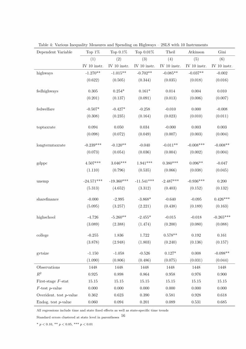
Table 4: Various Inequality Measures and Spending on Highways – 2SLS with 10 Instruments

Dependent Variable Top 1% Top 0.1% Top 0.01% Theil Atkinson Gini(1) (2) (3) (4) (5) (6)

IV 10 instr. IV 10 instr. IV 10 instr. IV 10 instr. IV 10 instr. IV 10 instr.highways -1.270** -1.015** -0.702** -0.085** -0.037** -0.002

(0.622) (0.505) (0.344) (0.035) (0.018) (0.016)

fedhighways 0.305 0.254* 0.161* 0.014 0.004 0.010(0.201) (0.137) (0.091) (0.013) (0.006) (0.007)

fedwelfare -0.507* -0.427* -0.258 -0.010 0.000 -0.008(0.308) (0.235) (0.164) (0.023) (0.010) (0.011)

toptaxrate 0.094 0.050 0.034 -0.000 0.003 0.003(0.098) (0.072) (0.049) (0.007) (0.003) (0.004)

longtermtaxrate -0.239*** -0.120** -0.040 -0.011** -0.008*** -0.008**(0.073) (0.054) (0.036) (0.004) (0.002) (0.004)

gdppc 4.507*** 3.046*** 1.941*** 0.380*** 0.096** -0.047(1.110) (0.796) (0.535) (0.066) (0.038) (0.045)

unemp -24.571*** -19.360*** -11.541*** -2.487*** -0.936*** 0.200(5.313) (4.652) (3.312) (0.403) (0.152) (0.132)

sharefinance -0.000 -2.995 -3.868* -0.640 -0.095 0.426***(5.095) (3.257) (2.221) (0.438) (0.189) (0.163)

highschool -4.726 -5.260** -2.455* -0.015 -0.018 -0.265***(3.089) (2.388) (1.474) (0.200) (0.080) (0.088)

college -0.255 1.836 1.722 0.578** 0.192 0.161(3.878) (2.948) (1.803) (0.240) (0.136) (0.157)

gvtsize -1.150 -1.058 -0.526 0.127* 0.008 -0.098**(1.090) (0.806) (0.486) (0.075) (0.031) (0.044)

Observations 1448 1448 1448 1448 1448 1448R2 0.925 0.898 0.864 0.958 0.976 0.900First-stage F -stat 15.15 15.15 15.15 15.15 15.15 15.15F -test p-value 0.000 0.000 0.000 0.000 0.000 0.000Overident. test p-value 0.362 0.623 0.390 0.581 0.928 0.618Endog. test p-value 0.060 0.094 0.201 0.089 0.531 0.685

All regressions include time and state fixed effects as well as state-specific time trends

Standard errors clustered at state level in parentheses

* p < 0.10, ** p < 0.05, *** p < 0.01

16

percentage points, which is not of trivial size. Given the second-stage estimate, this would translateinto an increase of the top 1% income share of about 6 percentage points within a time period oftwo years.

The negative correlation between state spending on highways and the number of appropriationscommittee members for that state turns out to be very significant, in agreement with earlier resultsby Knight (2002) who used membership in transportation committee. More recently, Dupor (2017)has documented a similar pattern in the context of the American Recovery and Reinvestment Act(ARRA), President Obama’s stimulus plan implemented at the outset of the Great Recession.5 Inaddition to the political-economy interpretation that Knight (2002) gives to the crowding-out effect,we conjecture that balanced-budget requirements that virtually all states have introduced in theirlegislative process are important to understand why additional federal funds generate cuts in bothspending and taxes. To flesh out such a simple idea, we now provide a reduced-form toy model thatillustrates how preference for tax cuts over public spending can lead to crowding-out under balanced-budget.6 Imagine that an hypothetical state governor has Stone-Geary-type preferences given byα log(I − I∗) − β(T − T ∗), where I stands for realized infrastructure investments, say, on highways,and T account for the taxes paid by the governor’s constituency. The starred variables I∗ and T ∗

stand for some corresponding baseline levels. Such preferences arise, for instance, if the probabilityfor the state governor to be elected goes up with state spending but down with taxes collected onstate residents’ incomes. In other words, spending more and taxing less improve the perspectiveof the incumbent candidate and governor in power to be elected or reelected. The state governor’sbudget constraint is given by I = T + F , where F is federal funding and is taken for simplicity asgiven by a given state. The governor then chooses I that maximizes α log(I − I∗) − β(T − T ∗),which delivers an optimal investment level given by Iopt = −αF/(β − α) + (βI∗ − αT ∗)/(β − α).Provided that the governor has a preference over taxing less relative to spending more (that is, ifβ > α), spending on infrastructure Iopt goes down when the state gets additional federal funding,that is, if F rises. The rationale for this is that optimal taxes, the expression of which is given byT opt = −βF/(β − α) + (βI∗ − αT ∗)/(β − α), also go down when F increases. In summary, thetrade-off between taxes and spending is resolved by reducing the former at the expense of a fall inthe latter.

In order to get a clearer understanding and a visual perspective of the data, showing the negativerelationship between the number of appropriations committee members and the level of investmenton highways, we discuss two noteworthy cases. In Figure 1, we plot both variables against time forthe state of Massachusetts. Both the number of seats in the appropriations committee and the (logof) of real spending on highways are shown to be flat from 1970 to 1990. However, both variables

5Leduc and Wilson (2017), however, find that crowding-out was absent in their analysis of the ARRA, presumablybecause the Great Recession forced states to implement policies aimed at stimulating the local economy, much likeARRA was designed as a federal stimulus package. In contrast, Knight (2002) analyzes the period from 1983 to 1997during which no commensurately large recession occurred.

6The following example builds upon a suggestion by Juan Antonio Montecino, whom the authors gratefully thank.

17

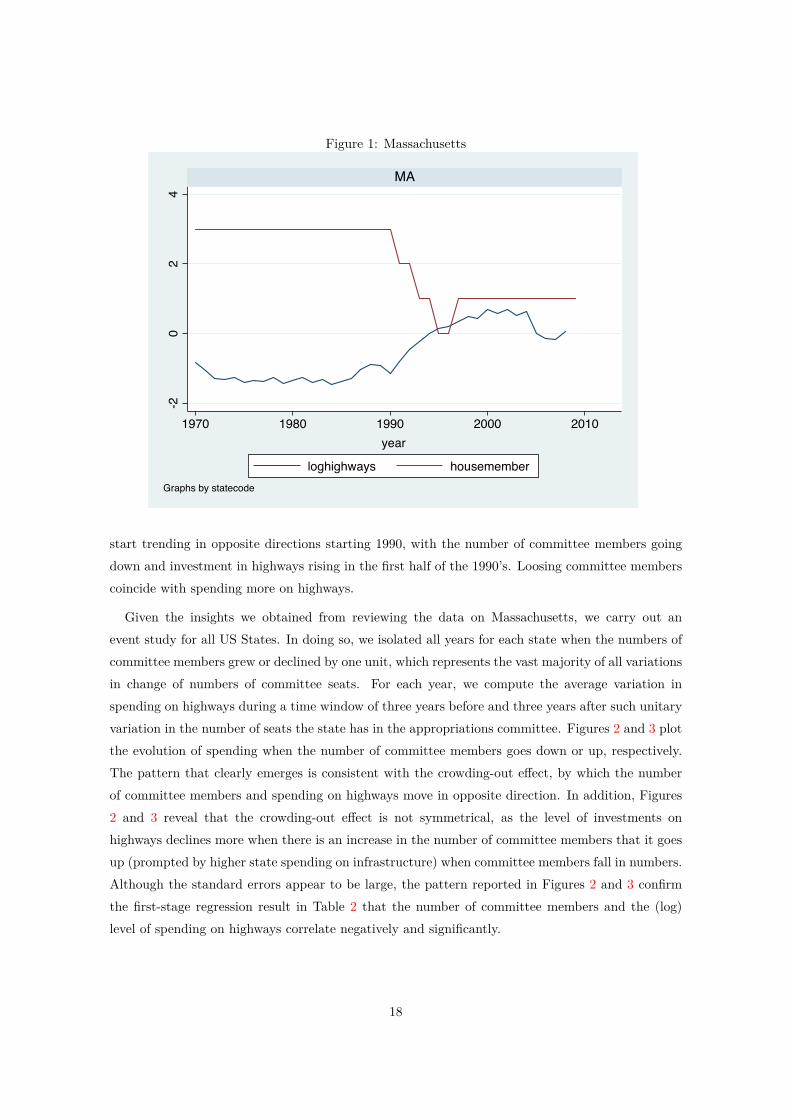
Figure 1: Massachusetts

-20

24

1970 1980 1990 2000 2010

MA

loghighways housemember

year

Graphs by statecode

start trending in opposite directions starting 1990, with the number of committee members goingdown and investment in highways rising in the first half of the 1990’s. Loosing committee memberscoincide with spending more on highways.

Given the insights we obtained from reviewing the data on Massachusetts, we carry out anevent study for all US States. In doing so, we isolated all years for each state when the numbers ofcommittee members grew or declined by one unit, which represents the vast majority of all variationsin change of numbers of committee seats. For each year, we compute the average variation inspending on highways during a time window of three years before and three years after such unitaryvariation in the number of seats the state has in the appropriations committee. Figures 2 and 3 plotthe evolution of spending when the number of committee members goes down or up, respectively.The pattern that clearly emerges is consistent with the crowding-out effect, by which the numberof committee members and spending on highways move in opposite direction. In addition, Figures2 and 3 reveal that the crowding-out effect is not symmetrical, as the level of investments onhighways declines more when there is an increase in the number of committee members that it goesup (prompted by higher state spending on infrastructure) when committee members fall in numbers.Although the standard errors appear to be large, the pattern reported in Figures 2 and 3 confirmthe first-stage regression result in Table 2 that the number of committee members and the (log)level of spending on highways correlate negatively and significantly.

18

Figure 2: Event Study – Fall in State Spending on Highways

.6.8

11.2

1.4

1.6

housem

ember

-.15

-.1-.05

0.05

.1loghighw

ays

-4 -2 0 2 4t

loghighways loghighways-s.d./loghighways+s.d.housemember

Figure 3: Event Study – Rise in State Spending on Highways.5

11.5

2housem

ember

-.1-.05

0.05

.1loghighw

ays

-4 -2 0 2 4t

loghighways loghighways-s.d./loghighways+s.d.housemember

19

4 Further Discussion

4.1 Inside the Black Box: the Role of the Construction Sector

Section 3 documents that the causal chain from rising spending on highways to inequality reduc-tion operates at horizons shorter than 2 years. This fact suggests that the construction sector mightbe important in channeling at least part of that causal effect. In line with such intuitive reasoning,we now provide suggestive evidence that rising spending on highways goes hand in hand with anincreasing wage paid by the construction sector.7 Figure 4 reports a scatter plot of our two variablesof interest that clearly reveals how spending on highways and the wage paid in the constructioncorrelates positively. Such eye-ball econometrics is formally confirmed by Table 5, which reportsregression results where the dependent variable is the construction wage. Column (1) in Table 5shows the coefficient of spending on highways when the dependent variable is the construction wageand both state and time fixed effects. Column (2) adds state-specific time trends, while column (3)further adds the unemployment rate and GDP per capita as covariates. All variables are highlysignificant and have the expected sign: the wage and the level of unemployment go in oppositedirections while the wage and the level of economic activity go hand in hand at the state level. Thepoint estimate indicates that a 1% increase in spending on highways is associated with an increasein the construction wage of about 5 basis points. Column (4) in Table 5 finally shows that spendingwith a one-year lag also correlates positively with the wage paid in the construction sector. This isconsistent with our findings in Section 3 that spending on highways affects income inequality withina couple of years.8

We are fully aware that the evidence reported above is only suggestive of the result that morespending on highways at the state level reduces income inequality through a booming constructionsector. To test further such an hypothesis, we would like to go beyond top shares and investigatewhich parts of the income distribution are most affected by investments in transportation infras-tructure. Our guess is that lower percentiles will be more impacted if it is indeed the case that moreconstruction jobs drive some people out of lower-pay jobs, thus reducing inequality. Unfortunately,the data on lower percentiles of the US income distribution at the state level is not yet available.9

7Our measure of the wage in the construction sector comes is constructed from BEA data. We divide the wagesand salaries by employment (respectively series SA7 and SA25, available in the Annual State Personal Income andEmployment section at https://www.bea.gov/regional/index.htm), both from the private non-farm constructionsector.

8In addition, unreported results show that all the indices of income inequality we use correlate negatively withthe construction wage lagged one or two years. This provides further evidence that a rising wage in the constructionsector contributes to inequality reduction.

9Private correspondence with Estelle Sommeiller in February 2018 suggests that such data will eventually becomepart of the Wealth and Income Database, though.

20

Figure 4: Wage in Construction Sector and Spending on Highways

-20

24

6w

age

in c

onst

ruct

ion

sect

or (

in lo

g)

-3 -2 -1 0 1 2spending on highways (in log)

4.2 Policy Implications

A particular feature that emerges from the empirical results discussed in Section 3 is that acces-sion of a particular elected representative from, say, the state of California to the AppropriationsCommittee is largely exogenous to the economic situation to his or her state. The reason being isthat newly available seat is withdrawn from another state, for example, such as Wisconsin, due toan existing committee member failing to be re-elected or to loss of life. Either way, the vacancythat was filled by a Californian representative, largely because of partisan balance and seniority inthe House, is almost a random assignment since it has nothing to do with the level of inequality inCalifornia or with any other economic outcome in California for that matter. This is why IV esti-mation is attractive given our data to uncover a possible causal effect from infrastructure spendingto income inequality. The two-step chain in the IV estimation delivers stark results. In the firststage, as reported in Section 3.2, the number of committee members in a particular state turns outto be a rather good instrument for spending on highways in that particular state. This outcome isin agreement with the earlier empirical literature (Knight, 2002), which has shown that getting anadditional committee member in the transportation authorization committee triggers federal grantsto finance expenditures on highways that, in turn, typically leads to a reduction of state spendingon highways, the so-called “crowding-out” effect.10 As mentioned earlier, the fact that almost allstates have balanced-budget constraints is probably important to understand why on average theaddition of a new committee member leads to a cut in state spending. From the second-stage re-

10See for example Bradford and Oates (1971) for an early political-economy model of the crowding-out effect offederal grants on state spending.

21

Table 5: Wage in Construction Sector and Spending on Highways

Dependent Variable Wage in Construction Sector(1) (2) (3) (4)OLS OLS OLS OLS

highways 0.087*** 0.076*** 0.049*** 0.038***(0.020) (0.016) (0.016) (0.013)

L.highways 0.014**(0.007)

L2.highways 0.004(0.008)

unemp -1.389*** -1.422***(0.330) (0.336)

gdppc 0.455*** 0.454***(0.109) (0.109)

Observations 1598 1598 1598 1598R2 0.947 0.967 0.978 0.978State-specific time trends no yes yes yes

All regressions include time and state fixed effects

Standard errors clustered at state level in parentheses

* p < 0.10, ** p < 0.05, *** p < 0.01

sults detailed in Section 3.1, we learn that the crowding-out effect has adverse effects on incomeinequality: when the representative from California gets appointed on the committee, the state ofCalifornia slashes spending on highways within a few years. As a consequence, jobs are lost in theconstruction sector and people who are fired end up in a lower position in the income distribution.At the end of such a causal chain, therefore, a reduction in the spending on highways leads to anincrease in income inequality. Of course, the mechanism works both ways. For example, the caseof Massachusetts illustrated in Figure 1 shows that the loss of committee members for that statein the 1990s triggered a significant increase in spending on highways, which was accompanied by areduction in the income share of the top 1%.

We believe that some important policy implications can be drawn from our main empirical results.First, in the context of the US, our analysis reveals that there are adverse effects of federal fundingthrough appropriations committees. As summarized above, the existence of a crowding-out effectmeans that an additional committee member translates into lower state spending on highways,which in turn causes rising inequality. This suggests that there are several problems associated

22

with the indirect allocation of federal grants through congressional committees. Nothing preventsstates to cut their spending when they get additional funding from the federal government, andboth our analysis and anecdotal evidence suggest that there are large incentives to pursue suchas path. In other words, unless the allocation process imposes some clauses that forbid recipientstates to slash their spending when they receive federal grants, the causal chain described abovewill operate. Surprisingly enough, such no-spending-cut constraints have sometimes been imposedbut not consistently over time or over spending items. For example, Dupor (2017) discusses thisissue in the context of the American Recovery and Reinvestment Act that started in 2009, andreports that a no-spending-cut clause applied to the education leg of the stimulus plan but not tothe funds allocated for investment on highways. There is no clear reason why this was the case butit stands to reason to assume that the arguments in favor of similar clauses should not differ muchdepending on the spending item that is financed by the federal budget. And similarly, of course,cases against such rules, for example because discretion should be preferred over strict rules in thecontext of state spending, should not depend on which item the money is spent on. In addition,one possible limitation of allocating federal grants through appropriation committees is that it isin effect a zero-sum game: by construction, when one state wins a seat, another state loses a seat.This means that getting or loosing political accession to such committees might create unnecessaryrandomness in state spending that have large economic effects, such as investment in transportationinfrastructure. Imposing explicit no-spending-cut clauses, however, would help to mitigate thissource of uncertainty.

Grants from national governments to sub-national administrative bodies are not unique featuresthat characterize industrially advanced countries. It is very plausible that low-income developingeconomies also possess similar patterns. Substantiating such a claim is however beyond the scopeof this study. Nonetheless, such a reasonable assumption suggests that our methodology could inprinciple be helpful to measure the extent to which investments in infrastructure have a causalimpact on income inequality and on the dispersion of other key social indicators such as health andeducation. In view of our case study based on US data, to make sure that federal spending has desiredeffects, as opposed to unintended adverse outcomes at a local level, greater transparency should beimposed. One possible policy measure that would contribute towards meeting this objective at anational and global level is the development of infrastructure investment platforms.11 The ideais that web-based, open-access platforms where infrastructure needs and sources of funding arematched could provide enough transparency to ensure that local governments actually spend themoney where they should. Most importantly, such investment platforms would help to monitorpossible leakages and other losses due to corruption.12. The benefits of enhancing transparency areobvious for the potential beneficiaries of such investments, a large fraction of whom live in countries

11See Section 5.2 in Hooper et al. (2017) and the references therein for a more detailed discussion of investmentplatforms.

12An illuminating discussion of the former aspect in the context of a cost-benefit analysis of electrification projectsin Africa appears in Lee et al. (2016).

23

where the level of democratic accountability is unfortunately low. To the extent that the future liesin the development of Public Private Partnerships to finance the gigantic infrastructure investmentgap around the world (see Arezki et al., 2017), such platforms would also make infrastructure amore attractive asset class for global investors, especially at times of extremely low returns on safeasset, particularly following the aftermath of the 2008 financial crisis. All these aspects are possiblyrelevant to think about policies that would foster investments in infrastructure in many developingeconomies and should as such be the topics of further research and fieldwork.

5 Conclusion

To the best of our knowledge, this paper is the first of its kind which shows a causal relationshipbetween investment on highways and income inequality by employing US state-level data from 1976to 2008. We carried out IV estimations to test for causality, not because we subscribed to the viewthat members from each state in the US House of Representatives Committee on Appropriations(HRCA) would have a direct impact on income inequality. Instead we wanted to empirically examinewhether the HRCA would have an indirect effect through federal funding on highways spending ata state level. Our results are consistent with earlier research work by Aghion et al. (2009,2016),showing that state membership in the Senate committee on appropriations is a better instrumentthan membership in other types of authorization committees. A contribution of our paper to thisliterature is twofold. Firstly, we show that accession to the HRCA by an elected member from agiven state is, on average, accompanied by a reduction in state level spending on highways. Secondly,we show that decreasing state level spending on highways causes income inequality to rise over aperiod of just a few years.

One of the main aims of this paper has been to empirically test whether infrastructure investmentscan reduce inequality, and thus facilitate long-term sustainable growth. An important question thatwe have largely left from our analysis is whether infrastructure investments can generate economicgrowth over the short term. A recent World Bank study (2015) points to infrastructure investmentsas being the main driver behind the notable increase (approximately 50 percent) in economic growthin Sub-Saharan Africa over the past decade. The same study also attributes approximately a 6percent rise in growth of real income in China in 2007 to infrastructure spending from 1990-2005(amounting to US$600 billion) to upgrade roads and to build expressway networks to link all of thelarge cities in the country. Further examples cited in the World Bank Report about infrastructuredevelopment serving as an effective policy mechanism to generate economic growth, include theUS$1 trillion earmarked by India for infrastructure development up to 2020. Indirectly, however,we argue that reducing inequality through infrastructure investments - even when the economy ison a stable path - can produce long term sustainable growth, as opposed to short term growththrough government stimulus programs during economic downturns. The concept of inequality isrelatively easy to grasp, but the real challenge lies in being able to implement appropriate policy

24

measures and to empirically test their impact on long sustainable economic growth, or to determinewhether causation runs in the opposite direction. The relationship between inequality and economicgrowth continues to be a contentious issue. The early work by Simon Kuznets (1955), for example,claims that income inequality increases during early stages of economic development, generatedby industrialization and that this process declines at later stages. Kaldor (1960) too argues thatcountries are confronted with a tradeoff between achieving economic growth and reducing inequality.This view was widely held amongst economists five decades ago (cited in Bahety et al. 2012). Fields(2001) however argues that the inverted “U”-shaped Kuznets curve is not backed up by empiricaldata. Instead, he maintains that the type of economic growth is what determines whether inequalityincreases or declines over time, as opposed to stages of industrial development. In sum, Kanburand Stiglitz (2015) argue that the earlier Kuznets and Kaldor models are outdated in the currentcontext of the global economy. They write that “the new models need to drop competitive marginalproductivity theories of factor returns in favor of rent-generating mechanism and wealth inequalityby focusing on the rules of the game.” A limitation of this paper is that the impact on shortterm growth from infrastructure investments is largely left out of the discussion. In principle, ourinstrument could also be used to test whether spending on highways also affects growth in a positivemanner. While it is simply beyond the scope of this paper to take on this task, a promising extensionwould be tackle the question of whether spending on infrastructure fosters inclusive growth. Morespecifically, from a policy-making perspective, a pressing issue is to shed light on the extent to whichthe lack of investment in infrastructure may be one channel through which inequality hurts growth.

To check the external validity of our results, it would be natural to test whether infrastructurespending of other types, most prominently education and health, could also reduce inequality and atthe same time promote growth, through increasing human capital. Using cross country data wouldhelp to assess to what extent the causal effect is also prevalent in other developed as well as low-income developing economies. Although our case study is based on US data, the results may shedlight on limitations to allocate national funds to sub-national governments. Efficient decentralizationof spending on infrastructure is a challenging issue in many emerging and developing economies, notto mention the financing of infrastructure. One possible way to address both issues jointly could bethe design and careful implementation of investment platforms that both attract global investorsand improve transparency. As a consequence, such platforms have the potential to help generateand greatly enhance the impact of investments on infrastructure for reducing inequality and at thesame time generating economic growth.

25

A Appendix

A.1 US House of Representatives Committee on the Appropriations

The purpose of this appendix is to provide more details on the source of the data we use aswell as on the role and nomination process of the US House of Representatives Committee OnAppropriations, which is “accountable for responsible, limited levels of federal discretionary spend-ing” (see http://appropriations.house.gov/). First, the data have been collected by GarrisonNelson (Committees in the U.S. Congress, 1947-1992, House Committees 80th-102nd Congress)and Charles Stewart III and Jonathan Woon (Congressional Committee Assignments, 1993-2017,House Membership Data 103rd to 114th Congresses), and they are available from Charles Stewart’scongressional data page at http://web.mit.edu/17.251/www/data_page.html. Figure 5 plots thedata over time for all states except Wyoming, which has no representation in the House committeeon appropriation, to ease exposition.13

Edwards and Stewart (2006) find that the Committee on Appropriations is the second mostpowerful committee in the House of Representatives, while the Committee on Transportation andInfrastructure is ranked only 10th. We believe this fact helps understand why earlier papers usingmembership in the latter committee (Knight, 2006, Feyrer and Sacerdote, 2011, Leduc and Wil-son, 2017) have found that such measure of congressional power is not a very strong instrument,in particular for highway grants. In contrast, results by Aghion et al. (2009,2016) and our ownanalysis both find that the number of state senators and representatives in the committees on ap-propriations is a powerful instrument to identify exogenous variations in innovation and in statespending on highways, respectively. As a matter of fact, institutional details shed light on thefindings by Edwards and Stewart (2006) that appropriations committees are much more powerfulthan other standing committees, such as the one on transportation and infrastructure. As describedin Streeter (2008, summary and p. 1), “Appropriations measures are under the jurisdiction of theHouse and Senate Appropriations Committees. These measures provide only about 40% of totalfederal spending for a fiscal year. The House and Senate legislative committees control the rest. [...]When considering appropriations measures, Congress is exercising the power granted to it underthe Constitution, which states, ‘No money shall be drawn from the Treasury, but in Consequenceof Appropriations made by Law.’ [...] Congress has also established an authorization-appropriationprocess that provides for two separate types of measures-authorization bills and appropriation bills.These measures perform different functions and are to be considered in sequence. First, authoriza-tion bills establish, continue, or modify agencies or programs. Second, appropriations measures mayprovide funding for the agencies and programs previously authorized.” In other words, the commit-tee on transportation grants or extends authorizations for programs and agencies to be funded, butit is the committee on appropriations that decides over the amount of effective funding and has even

13Note that, as expected, the significance of our 2SLS estimates improves when we drop the 7 states with norepresentation in the House appropriations committee, but not by much.

26

Figure 5: Number of Members in US House Committee On Appropriations – 1970 to 20080

24

68

02

46

80

24

68

02

46

80

24

68

1970 1980 1990 2000 2010 1970 1980 1990 2000 2010 1970 1980 1990 2000 2010 1970 1980 1990 2000 2010 1970 1980 1990 2000 2010

AK AL AR AZ CA

CO CT DC DE FL

GA HI IA ID IL

IN KS KY LA MA

MD ME MI MN MO

hous

emem

ber

year

02

46

02

46

02

46

02

46

02

46

1970 1980 1990 2000 2010 1970 1980 1990 2000 2010 1970 1980 1990 2000 2010 1970 1980 1990 2000 2010 1970 1980 1990 2000 2010

MS MT NC ND NE

NH NJ NM NV NY

OH OK OR PA RI

SC SD TN TX UT

VA VT WA WI WV

hous

emem

ber

year

27

power to create unauthorized funding: “[A]n unauthorized appropriation is new budget authority inan appropriations measure (including an amendment or conference report) for agencies or programswith no current authorization, or whose budget authority exceeds the ceiling authorized.” (Streeter,2008, p. 22). A further sign of relative strength is the fact that the number of Appropriationssubcommittees is more than two times larger than the number of Transportation subcommittees.In addition, the House committee on appropriations has had a first-mover advantage, compared tothe Senate’s: “[T]raditionally, the House of Representatives initiated consideration of regular appro-priations measures, and the Senate subsequently considered and amended the House-passed bills”(Streeter, 2008, p. 5). Our conclusion is that using membership in the committee on appropriationsprovides a better measure for the congressional power to grant federal funding to states, comparedto membership in authorization committees such as the committee on transportation, which areaccordingly less valued by senators or representatives as empirically shown by Edwards and Stewart(2006).

A precise account of the nomination process that drives accession to the committee on appropri-ations is beyond the scope of this paper. However, we would like to stress the fact that seniorityrules are the most important factor behind nomination, when a new seat becomes available. Ed-wards and Stewart (2006, p. 8) report that republican members are “assigned to committees by theRepublican Conference’s Committee on Committees. Votes on this committee were weighted by thesize of each state’s congressional delegation and assignments were typically based on the senioritysystem”. Democrats, on the other hand, are selected by a vote system held by the Democratic Steer-ing and Policy Committee. The overall nomination system is therefore largely based on seniorityand partisan loyalty. However, while Congress rules are rather transparent about how nominationsare to be formally approved, it does not seem that such rules make explicit how nominations tocommittees are to be made.

A.2 2SLS Estimation with Various Lags

In Table 6 we report results from regressions in which both the endogenous regressor - the spendingon highways - and the instrument - the number of committee members - take different lags thatare indicated in the first two rows for the former and in the columns for the latter. To save space,the covariates that turn out to be not significant do not appear. In addition, unreported estimatesshow that similar results occur when a two-year lag applies to spending on highways. All in all, weconclude that the inequality-reducing effect of spending on highways operates over a couple of yearsat most.

28

A.3 2SLS Estimation with Spending on Education and Lagged Inequality

In Table 7 we report results from regressions in which state spending and federal funding forhigher education (in the first three columns) and lagged inequality (in the last three columns) areadded to our benchmark specification as further controls. Results are similar to those in Table 1,except for a slightly weakened effect of highways on the top 1% share when lagged inequality isadded (the p-value goes from slightly below to slightly above 5% though). While the coefficient onlagged inequality is significant, quite unsurprisingly, that of contemporaneous spending on highereducation is not. However, unreported results show that lagged spending on higher education isnegatively correlated with income inequality, which is in line with previous analysis in Hooper et al.(2017), while our main result is unchanged. In other words, accounting for the inequality reductioneffect of spending on higher education, it is still the case that more spending on highways causestop income shares to go down.

A.4 Searching for Violations of the Exclusion Restriction

A possible concern with our empirical strategy is that the instrument we use - the number of staterepresentatives in the Appropriations Committee - could have a direct effect on income inequality.This could happen for instance if accession to the committee is more easily granted for houserepresentatives who support pro-inequality policies, which would be consistent with the result thatadditional committee members cause inequality to increase. To search for such potential violationsof the exclusion restriction, we have extensively experimented with subsamples of our data, whenshorter time spans or smaller subsets of states are considered. We haven’t found any worryinginstance with both a significant reduced form and a zero first stage. In Tables 8-9 we report randomoutcomes of our search, where the absence of a statistically significant first-stage implies no evidenceof a corresponding reduced-form estimate for the instrument related to the number of committeemembers. In Table 8 we report results obtained over the period from 1985 to 1995, while Table9 relates to a subsample of 15 states (with codes between 10 and 25, all states being ranked inalphabetical order).

29

Table 6: Top 1% Income Share and Spending on Highways – 2SLS with Various Lags

Dependent Variable Top 1% Income Share(1) (2) (3) (4) (5)

IV 1 instr. IV 1 instr. IV 1 instr. IV 1 instr. IV 1 instr.L3.hm L2.hm L1.hm L3.hm L2.hm

highways -3.498** -4.147** -4.436*(1.713) (2.038) (2.409)

L1.highways -3.703* -3.652*(2.023) (1.994)

fedhighways 1.130* 1.363* 1.468* 0.767 0.754(0.612) (0.727) (0.816) (0.469) (0.459)

fedwelfare -0.848** -0.930** -0.957* -1.113** -1.105**(0.404) (0.468) (0.527) (0.469) (0.494)

toptaxrate 0.188* 0.193* 0.204* 0.252** 0.250**(0.106) (0.113) (0.119) (0.129) (0.126)

longtermtaxrate -0.209** -0.199** -0.195** -0.258*** -0.258***(0.090) (0.096) (0.099) (0.097) (0.095)

gdppc 4.588*** 4.852*** 5.071*** 4.258** 4.236**(1.617) (1.843) (1.947) (1.770) (1.756)

unemp -21.601*** -23.001*** -22.551*** -18.214*** -18.237***(5.164) (5.709) (6.209) (5.778) (5.581)

Observations 1598 1598 1598 1648 1648R2 0.912 0.900 0.894 0.895 0.896First-stage F -stat 6.87 5.94 5.11 5.46 6.02F -test p-value 0.011 0.018 0.028 0.023 0.017Endog. test p-value 0.045 0.028 0.024 0.065 0.043

All regressions include time and state fixed effects as well as state-specific time trends

Controls that are not significant are not reported. Standard errors clustered at state level in parentheses

* p < 0.10, ** p < 0.05, *** p < 0.01

30

Table 7: Top Shares and Highways – 2SLS with Spending on Education and Lagged Inequality

Dependent Variable Top 1% Top 0.1% Top 0.01% Top 1% Top 0.1% Top 0.01%(1) (2) (3) (4) (5) (6)

IV 1 instr. IV 1 instr. IV 1 instr. IV 1 instr. IV 1 instr. IV 1 instr.highways -4.216** -3.447* -2.467* -2.635* -2.084* -1.544*

(2.115) (1.830) (1.288) (1.403) (1.201) (0.832)

highered 0.372 0.233 0.187(1.019) (0.771) (0.526)

fedhighered 0.403 0.196 0.041(0.402) (0.290) (0.182)

L1.top1% 0.406***(0.054)

L1.top0.1% 0.439***(0.050)

L1.top0.01% 0.438***(0.044)

fedhighways 1.390* 1.145* 0.810* 0.906* 0.731* 0.531*(0.751) (0.645) (0.461) (0.485) (0.410) (0.289)

fedwelfare -0.966** -0.824** -0.553** -0.456 -0.371* -0.251(0.474) (0.336) (0.246) (0.314) (0.213) (0.154)

toptaxrate 0.202* 0.179* 0.118* 0.122 0.104* 0.069*(0.118) (0.098) (0.067) (0.075) (0.058) (0.039)

longtermtaxrate -0.200** -0.100 -0.025 -0.133** -0.064 -0.015(0.095) (0.070) (0.048) (0.063) (0.044) (0.031)

gdppc 4.819*** 3.292** 2.151** 2.695** 1.716* 1.201*(1.682) (1.283) (0.842) (1.324) (1.028) (0.649)

unemp -22.479*** -18.278*** -11.875*** -17.020*** -13.387*** -8.460***(5.815) (5.201) (3.858) (4.198) (3.707) (2.725)

Observations 1598 1598 1598 1598 1598 1598R2 0.899 0.857 0.787 0.934 0.911 0.870First-stage F -stat 5.65 5.65 5.65 5.72 5.46 5.43F -test p-value 0.021 0.021 0.021 0.020 0.023 0.023Endog. test p-value 0.026 0.068 0.063 0.052 0.094 0.065

All regressions include time and state fixed effects as well as state-specific time trends

Controls that are not significant are not reported. Standard errors clustered at state level in parentheses

* p < 0.10, ** p < 0.05, *** p < 0.01

31

Table 8: Reduced Form and First Stage – 1985-1995

Dependent Variable Top 1% Top 1% Top 1% highways highways highways(1) (2) (3) (4) (5) (6)OLS OLS OLS OLS OLS OLS

L2.housemember 0.097 0.014 -0.018 0.001(0.094) (0.095) (0.032) (0.028)

L6.highways 0.173 0.173 -0.218*** -0.218***(0.158) (0.158) (0.042) (0.042)

fedhighways -0.334 -0.382 -0.381 0.447*** 0.446*** 0.446***(0.255) (0.257) (0.260) (0.087) (0.064) (0.064)

fedwelfare -0.209 -0.169 -0.171 0.091 0.110 0.109(0.345) (0.360) (0.361) (0.135) (0.121) (0.120)

toptaxrate 0.018 0.021 0.021 0.002 -0.005 -0.005(0.087) (0.086) (0.086) (0.030) (0.024) (0.024)

longtermtaxrate -0.186*** -0.170*** -0.170*** 0.016 0.002 0.002(0.059) (0.062) (0.062) (0.024) (0.022) (0.022)

gdppc 5.428*** 5.803*** 5.801*** 0.656* 0.091 0.091(1.178) (1.122) (1.122) (0.373) (0.359) (0.360)

unemp -28.003*** -25.271*** -25.294*** 0.971 0.373 0.370(5.513) (5.081) (5.062) (1.572) (1.640) (1.644)

sharefinance -2.221 0.144 0.022 0.249 -0.171 -0.184(6.086) (6.457) (6.353) (1.255) (1.041) (1.009)

highschool 0.152 0.386 0.351 0.149 0.457 0.453(2.426) (2.327) (2.276) (0.658) (0.623) (0.604)

college 6.360 7.949* 7.906* 1.831* 0.426 0.421(4.491) (4.638) (4.709) (0.981) (1.006) (1.001)

gvtsize 1.791 3.229 3.138 -1.621 -0.374 -0.383(7.052) (7.132) (7.187) (3.240) (2.664) (2.619)

Observations 550 550 550 550 550 550R2 0.820 0.826 0.826 0.668 0.727 0.727

All regressions include time and state fixed effects as well as state-specific time trends

Standard errors clustered at state level in parentheses

* p < 0.10, ** p < 0.05, *** p < 0.01 32

Table 9: Reduced Form and First Stage – 15 States

Dependent Variable Top 1% Top 1% Top 1% highways highways highways(1) (2) (3) (4) (5) (6)OLS OLS OLS OLS OLS OLS

L2.housemember 0.124 0.099 -0.025 -0.008(0.077) (0.069) (0.026) (0.019)

L6.highways 0.393 0.387 -0.044 -0.044(0.311) (0.313) (0.046) (0.045)

fedhighways 0.037 0.145 0.152 0.249*** 0.186*** 0.185***(0.073) (0.113) (0.113) (0.089) (0.065) (0.065)

fedwelfare -0.553* -0.576 -0.553 -0.296* -0.220 -0.222(0.316) (0.411) (0.398) (0.168) (0.138) (0.139)

toptaxrate -0.341*** -0.339** -0.325** 0.068** 0.042 0.041(0.101) (0.134) (0.128) (0.028) (0.036) (0.036)

longtermtaxrate 0.059 0.053 0.045 -0.023 -0.022 -0.021(0.100) (0.065) (0.063) (0.026) (0.028) (0.028)

gdppc 1.543 3.313** 3.240** 0.278 0.108 0.114(1.477) (1.671) (1.633) (0.351) (0.288) (0.285)

unemp -22.539*** -32.092*** -32.015*** 0.522 -0.651 -0.658(6.598) (7.266) (7.132) (1.777) (1.148) (1.145)

sharefinance 1.667 6.290 6.103 0.532 -0.173 -0.157(6.218) (6.373) (6.183) (1.628) (1.266) (1.267)

highschool -2.753 0.651 0.625 -0.359 -0.794 -0.791(4.113) (5.048) (5.103) (0.984) (0.908) (0.906)

college -3.943 -4.659 -4.998 0.209 0.725 0.754(5.972) (5.585) (5.719) (1.535) (1.500) (1.472)

gvtsize -1.259 -1.449 -1.525 0.262 0.087 0.093(1.391) (1.333) (1.344) (0.270) (0.156) (0.159)

Observations 510 462 462 510 462 462R2 0.948 0.939 0.939 0.809 0.831 0.831

All regressions include time and state fixed effects as well as state-specific time trends

Standard errors clustered at state level in parentheses

* p < 0.10, ** p < 0.05, *** p < 0.01 33

References

[1] Aghion P., L. Boustan, C. Hoxby, and J. Vandenbussche (2009). The Causal Impact of Educa-tion on Economic Growth: Evidence from U.S. Mimeo Harvard University.

[2] Aghion P., U. Akcigit, A. Bergeaud, R. Blundell, and D. Hémous (2016). Innovation and TopIncome Inequality. NBER Working Papers 21247.

[3] Arezki, R., P. Bolton, S. Peters, F. Samama, and J. Stiglitz (2017). From Global Savings Glut toFinancing Infrastructure: the Advent of Investment Platforms. Economic Policy, 32: 221-261.

[4] Atkinson, A., F. Bourguignon, Eds. (2015). Handbook of Income Distribution. Elsevier.

[5] Bahety, G., Y. Giesing, E. Kayihan, F. Lima, T. Oesche, and Q. Xue (2012). The CausalRelationship Between Inequality and Growth: Literature Review. OECD.

[6] Baum-Snow, N. (2007). Did Highways Cause Suburbanization? Quarterly Journal of Eco-nomics, 122: 775-805.

[7] Bénabou, R. (1996). Inequality and Growth, in Bernanke, B., and J. Rotemberg (Eds.), NBERMacroeconomics Annual.

[8] Bradford, D., and W. Oates (1971). The Analysis of Revenue Sharing in a New Approach toCollective Fiscal Decisions. Quarterly Journal of Economics, 85: 416-39.

[9] Chernozhukov, V., and C. Hansen (2008). The Reduced Form: a Simple Approach to Inferencewith Weak Instruments. Economics Letters, 100: 68-71.

[10] Cohen, L., J. Coval, and C.J. Malloy (2011). Do Powerful Politicians Cause Corporate Down-sizing? Journal of Political Economy, 119: 1015-1060.

[11] Dupor, B. (2017). So, Why Didn’t the 2009 Recovery Act Improve the Nation’s Highways andBridges? Federal Reserve Bank of St. Louis Review, 99: 169-82.

[12] Duranton, G., and M.A. Turner (2012). Urban Growth and Transportation. Review of EconomicStudies 79: 1407-1440.

[13] Edwards, K., and C. Stewart III (2006). The Value of Committee Assignments in Congresssince 1994. Unpublished MIT mimeo.

[14] Fernald, J. G. (1999). Roads to Prosperity? Assessing the Link Between Public Capital andProductivity. American Economic Review, 89: 619-638.

[15] Feyrer, J., and B. Sacerdote (2011). Did the Stimulus Stimulate? Real Time Estimates of theEffects of the American Recovery and Reinvestment Act. NBER Working Paper 16759.

34

[16] Fields, G.S. (2001) Distribution and Development: A New Look at the Developing World.Russell Sage Foundation, New York: The MIT Press.

[17] Forbes, K. (2000). A Reassessment of the Relationship Between Inequality and Growth. Amer-ican Economic Review, 90: 869-887.

[18] Frank, M. (2009). Inequality and Growth in the United States: Evidence from a New State-Level Panel of Income Inequality Measure. Economic Inquiry, 47: 55-68.

[19] Frank, M., E. Sommeiller, M. Price, and E. Saez (2015). Frank & Sommeiller & Price Series forTop Income Shares by US State since 1917. WID.world Technical Note Series, NÂ◦ 2015/7.

[20] Hooper, E., S. Peters, and P. Pintus (2017). To What Extent Can Long-Term Investments inInfrastructure Reduce Inequality? Banque de France Working Papers 624.

[21] Kaldor, N. (1960). Essays on Value and Distribution. Glencoe, Free Press.

[22] Kanbur, R., and J. Stiglitz (2015). Wealth and Income distribution: New Theories Needed fora New Era. VOX, CEPR’s Policy Portal. 18 August.

[23] Knight, B. (2002). Endogenous Federal Grants and Crowd-out of State Government Spending:Theory and Evidence from the Federal Highway Aid Program. American Economic Review,92: 71-92.

[24] Kuznets, S. (1955). Economic Growth and Income Inequality. American Economic Review, 45:1-28.

[25] Leduc, S., and D. Wilson (2017). Are State Governments Roadblocks to Federal stimulus? Evi-dence on the Flypaper Effect of Highway Grants in the 2009 Recovery Act. American EconomicJournal: Economic Policy, 9: 253-292.

[26] Lee, K., E. Miguel, and C. Wolfram (2016). Experimental Evidence on the Demand for andCosts of Rural electrification. Working Paper, University of California, Berkeley.

[27] Li, H., and H.-F. Zou (1998). Income Inequality is Not Harmful for Growth: Theory andEvidence. Review of Development Economics, 2: 318-34.

[28] Michaels, G. (2008). The Effect of Trade on the Demand for Skill: Evidence from the InterstateHighway System. Review of Economics and Statistics, 90: 683-701.

[29] Milanovic, B. (2016). Global Inequality, A New Approach for the Age of Globalization. HarvardUniversity Press.

[30] Nakamura, E., and J. Steinsson (2014). Fiscal Stimulus in a Monetary Union: Evidence fromUS Regions. American Economic Review 104: 753-792.

[31] Piketty, T. (2014). Capital in the 21st Century. Harvard University Press.

35

[32] Piketty, T., and E. Saez (2003). Income Inequality in the United States, 1913-1998. QuarterlyJournal of Economics, 118: 1-39.

[33] Redding, S., and M. Turner (2015). Transportation Costs and the Spatial Organization of Eco-nomic Activity. In (eds) Gilles Duranton, J. Vernon Henderson and William Strange, Handbookof Urban and Regional Economics, Chapter 20: 1339-1398.

[34] Streeter, S. (2008). The Congressional Appropriations Process: an Introduction. CongressionalResearch Service Report for the Congress 97-684.

[35] van der Weide, R., and B. Milanovic (2014). Inequality is Bad for Growth of the Poor. WorldBank Policy Research Working Paper Series 6963.

[36] World Bank (2015). Transformation Through Infrastructure, Infrastructure Strategy Update:FY 2012-2015. Washington, D.C.: World Bank Group.

36