1

The Causal Effect of Military Conscription on Crime and the Labor Market*

Randi Hjalmarsson† University of Gothenburg and CEPR

Matthew J. Lindquist††

SOFI, Stockholm University

February 3, 2016

Abstract This paper uses detailed individual register data to identify the causal effect of mandatory peacetime military conscription in Sweden on the lives of young men born in the 1970s and 80s. Because draftees are positively selected into service based on their draft board test performance, our primary identification strategy uses the random assignment of potential conscripts to draft board officiators who have relatively high or low tendencies to place draftees into service in an instrumental variable framework. We find that military service significantly increases post-service crime (overall and across multiple crime categories) between ages 23 and 30. These results are driven primarily by young men with pre-service criminal histories and who come from low socioeconomic status households. Though we find evidence of an incapacitation effect concurrent with conscription, it is unfortunately not enough to break a cycle of crime that has already begun prior to service. Analyses of labor market outcomes tell similar post-service stories: individuals from disadvantaged backgrounds have significantly lower income, and are more likely to receive unemployment and welfare benefits, as a result of service, while service significantly increases income and does not impact welfare and unemployment for those at the other end of the distribution. Finally, we provide suggestive evidence that peer effects may play an important role in explaining the unintended negative impacts of military service. Keywords: Conscription, Crime, Criminal Behavior, Draft, Military Conscription, Military Draft, Incapacitation, Labor Market, Unemployment. JEL: H56, J08, K42.

                                                            * We would like to thank seminar participants at the Swedish Institute for Social Research and the Tinbergen Institute for their helpful comments and suggestions. Hjalmarsson would also like to gratefully acknowledge funding support from Vetenskapsrådet (The Swedish Research Council), Grants for Distinguished Young Researchers. † University of Gothenburg, Department of Economics, Vasagatan 1, SE 405 30, Gothenburg, Sweden; randi.hjalmarsson@economics.gu.se †† Swedish Institute for Social Research (SOFI), Stockholm University, Universitetsvägen 10F, 106 91 Stockholm, Sweden; matthew.lindquist@sofi.su.se. 

2

1. Introduction

Young men in more than 60 countries around the world still face the prospect of mandatory

military conscription today.1 This occurs at a critical juncture in a young adult’s life – when

he is at the peak of the age-crime profile, making decisions about higher education, and

entering the labor market. It is thus not surprising that conscription remains a hotly debated

topic; in fact, a number of European countries have recently abolished it (France, 1996; Italy,

2005; Sweden, 2010; and Germany, 2011) while others have had failed referendums (Austria

and Switzerland in 2013).2 Yet, despite a growing body of academic literature, there is little

consensus about the impact of this potentially life transforming event.

The current paper contributes to this debate by utilizing individual administrative

records and a quasi-experimental research design to identify the causal impact of mandatory

military conscription in Sweden on crime, both concurrent with (incapacitation) and after

conscription. We complement this analysis by applying the same research design to legitimate

labor market outcomes, including education, income, and welfare and unemployment

benefits, as well as work-related health outcomes (sick days and disability benefits).

Mandatory military conscription in Sweden dates back to 1901 and was abolished in

2010, after a gradual decline that began upon the end of the Cold War. For most of this

period, all Swedish male citizens underwent an intensive drafting procedure upon turning 18,

including tests of physical and mental ability. These test results were reviewed by a randomly

assigned officiator, who determined whether the draftee would be enlisted. It is this

exogenous variation in the likelihood of serving generated by the randomly assigned officiator

that our analysis utilizes in an instrumental variable framework to identify the causal effect of

conscription on crime. In addition, for a subset of cohorts for whom we know the exact dates

                                                            1See the CIA’s World Factbook (https://www.cia.gov/library/publications/the-world-factbook/fields/2024.html) and http://chartsbin.com/view/1887 for a summary of this data. 2 Though the U.S. moved to an all-volunteer military in 1973, young men ages 18 to 26 are still required to register for the draft. Today, the US is debating extending this requirement to young women. http://www.nbcnews.com/news/us-news/military-officials-women-should-register-draft-n509851

3

of service, we also utilize a difference-in-difference matching framework to identify the

incapacitation effects of service.

There are a number of channels, many of which are opposing in nature, through which

military conscription may affect both contemporaneous and future criminal behavior. With

respect to the contemporaneous impacts, conscription may decrease criminal behavior through

an incapacitation channel, i.e. keeping young men otherwise engaged and isolated from

mainstream society. On the other hand, conscripted young men are not under 24-hour

supervision, and may still have the opportunity to commit crimes ‘after hours’; the increased

extent of social interactions that occur during conscription could even feasibly result in an

increased propensity to commit crimes that are highly ‘social’ in nature, like violent crimes.3

If conscription does “incapacitate” potential criminals, then this could potentially

result in a new path of lower criminal intensity; that is, post-service crime could be reduced

simply as a result of a decrease in crime contemporaneous with service. Alternatively, the

promotion of democratic values, which is one of the stated goals of mandatory conscription,

and the obedience and discipline training that one receives, may decrease post-service

criminal tendencies by helping to focus young men at this high risk age. Others argue that

exposure to weapons and desensitization to violence, especially during wartime conscription,

may exacerbate an individual’s criminal tendencies, particularly with respect to violent crime

(Grossman, 1995). Military conscription may also positively or negatively impact crime

through its impact on education and labor market outcomes. If conscription extends a young

males’ social networks, is viewed as a positive signal of quality by employers, or improves his

marketable skills (e.g. training as mechanics, truck drivers, cooks and medics), health, or

physical fitness, thereby improving labor market outcomes, then this could decrease the

propensity for crime (Becker, 1968). However, post-service crime may increase if

                                                            3 This parallels the school crime literature, where Jacob and Lefgren (2003) and Luallen ( 2006) have found an incapacitation effect of schooling on property crime but an exacerbating effect on violent crime, which they argue results from increased social interactions.

4

conscription interrupts a continuous educational path, delays entry into the labor market, and

reduces future labor market opportunities. Finally, exposure to a new peer group may have

either positive or negative effects on criminal behavior, depending on the relative

characteristics of the new and old peer groups; such peer effects could even lead to social

multiplier effects of conscription.

The existing research yields mixed results, with respect to both labor market and crime

outcomes. Angrist’s (1990) seminal study found that Vietnam draftees in the U.S. had lower

earnings than non-draftees; subsequent papers (Angrist and Chen, 2011; Angrist, Chen, and

Song, 2011) find that this gap closes over time, such that by age 50, draftees are on par with

non-draftees.4 With respect to peacetime service, Imbens and van der Klaauw (1995) find

lower wages for Dutch veterans, Grenet et al (2011) and Bauer et al (2009) find no impact on

wages for British and German cohorts coming of age just after the abolition of conscription,

and Card and Cardoso (2012) find a small positive effect on earnings for low-educated men in

Portugal.5 Bingley et al. (2014) find large earnings losses for high ability men in Denmark.

Two papers find a positive effect of conscription on labor market outcomes in the Swedish

context (Hanes et al. (2010) and Grönqvist and Lindqvist (2016)), but only the latter, which

focuses on officer training, seriously addresses the biases arising from the endogenous

selection process.6, 7

Few papers study the effect of conscription on crime in a quasi-experimental setting.8

Those studying Vietnam Veterans in the U.S. (taking advantage of differential exposure

                                                            4 Likewise, Siminski’s (2013) study of Australian Vietnam draftees finds a negative employment effect. 5 Maurin and Xenogiani (2007) use the abolition of conscription in France to study the effect of schooling on wages. 6 Using a regression discontinuity design, Grönqvist and Lindqvist (2016) find that officer training in the military significantly increases the probability of becoming a civilian manager. 7 Albrecht et al. (1999) also report regression coefficients that (in some specifications) show a positive return to military service in Sweden. But as their paper is about explaining the negative returns to time spent out of work (due to, e.g., maternity leave) and not about the effects of military service on earnings, they do not comment on these coefficients nor do they specifically address the issue of selection into military service. 8Beckerman and Fontana’s (1989) survey of the early criminology and psychology literature finds that Vietnam veterans do not have higher arrest rates than non-veterans. A handful of studies find a positive effect of being a

5

across cohorts to the draft (Rohlfs, 2010) or the draft board lottery (Lindo and Stoecker,

2012)) find some evidence that conscription causes an increase in violent crimes. Yet,

Siminski et al (2016) do not find an effect on violent crime in Australia during Vietnam era

conscription. Two papers consider the effects of peacetime conscription. In Argentina, where

males are randomly assigned eligibility based on the last three digits of their national identity

number, Galiani et al (2011) find that conscription increases crime, especially property and

white collar crimes, and decreases labor market outcomes; these effects are even larger for

wartime draftees. Finally, for a subset of the 1964 Danish birth cohort, Albaek et al.

(forthcoming) find that service reduces property crime among men with previous convictions

for up to four years (starting from the year in which they begin military service, which

typically lasts from 3 to 12 months). However, their data do not allow them to cleanly

estimate an incapacitation effect separately from a post-service effect.

The current paper addresses a number of limitations of the existing research. First, we

look at the effect of conscription on more modern cohorts who come of age in the 1990s,

nearly all previous research focuses on the Vietnam War or cohorts born in the 1950s and

1960s.9 Second, detailed individual register data allow us to study crimes committed when the

men are young adults (i.e. before the age of 30 for all cohorts), whereas most other papers

have been limited to studying crime committed after age 40 (Siminski et al, 2013; Galiani et

al, 2011). Given that crime has declined for many years on the age-crime profile by age 40

and the evidence that the earnings gap for draftees after the Vietnam War closes by age 50

(Angrist and Chen, 2011; Angrist, Chen, and Song, 2011), it is essential to study criminal

                                                                                                                                                                                          Vietnam Vet on violent crime, but these are often restricted to those in combat or individuals with mental health problems. See Yager et al (1984), Resnick et al (1989), and Yesavage (1983). 9 A recent exception is Anderson and Rees (2015), who study those deployed in the Iraq war from Fort Carson, Colorado from 2001 to 2009; they conclude that never-deployed units have a greater impact on crime and public safety than units recently returned from combat. Bingley et al. (2014) also study more recent cohorts of Danish men born 1976-1983. But their paper focuses on the labor market returns to military service. They do, however, report one interesting finding about crime when discussing the mechanisms that might drive the large negative effect on earnings that they find. They report a zero effect of military service on non-vehicular crime at the extensive margin for men aged 26-35. This zero holds for all quartiles of the ability distribution.

6

behavior in the short- and medium-terms rather than the long-term. Third, the Swedish

register data not only allows for more refined crime outcomes, but also one of the most

comprehensive analysis to date of the impact of peacetime service on a wide range of labor

market and health outcomes. Methodologically, as not all countries assign individuals to

service using a lottery system, we apply a new research design in the context of this literature

to identify the causal effects of service on crime. Finally, and in contrast to all of the existing

literature, information on the exact dates of service allows us to directly estimate the

incapacitation effects of service.

We begin with a sample non-immigrant males born between 1964 and 1990 from

Sweden’s Multigenerational Register (representing about 70% of the population), to which we

matched on longitudinal administrative records concerning income, education, tax records,

geographical location, criminal convictions, and draft board data. For individuals testing from

1990 to 1996, we can identify the officiators who reviewed the battery of draft board test

results and subsequently placed the draftees into service. Though we cannot identify

officiators for the 1997 to 2001 test cohorts, we do know their exact dates of service.

These key data features guide the two stages of our empirical analysis. The goal of the

first stage is to cleanly identify the causal effect of service on post-service crime. To deal with

the fact that conscripts are ‘selected’ into service on the basis of their draft board test

performance, we instrument for whether an individual serves with whether he is assigned to

an officiator with a high annual service rate (that is, an officiator whose annual share of

testees who serve is greater than the national share who serve in that year). We argue that this

instrument is both valid and relevant when conditioning on county by test year fixed effects.

With regards to the former, we provide both anecdotal and empirical evidence of random

assignment to officiators. With regards to the latter, we demonstrate that assignment to a high

service rate officiator increases the likelihood of service by almost eight percentage points,

7

with an appropriately high first-stage F-statistic. We also provide evidence that the necessary

monotonicity assumption holds.

The baseline results are striking: military service significantly increases both the

likelihood of crime and the number of crimes between ages 23 and 30; as all individuals in

our IV sample have completed service by age 23, this is a cleanly measured post-service

effect. Such a positive effect is actually seen across all crime categories, with especially

significant effects for violent crime, theft, drug and alcohol offenses, and other offenses. The

estimated effects are quite large, oftentimes more than twice the mean of the dependent

variable, and are driven by those with a criminal history prior to service or from low

socioeconomic status households. This heterogeneous impact of service is also seen with

respect to labor market outcomes. Individuals from disadvantaged backgrounds have

significantly lower income, and are more likely to receive unemployment and welfare

benefits. In contrast, military service significantly increases income and does not impact

welfare and unemployment for those at the other end of the distribution. There is no effect of

service on the likelihood of higher education. The only positive effect of service we see, at

least for those from disadvantaged backgrounds, is a decrease in disability benefits and the

number of sick days; these effects are in fact seen for all subsamples. We demonstrate the

robustness of our results to an alternative instrument (the leave out annual mean), a large set

of observable controls, and a falsification test that considers crime committed prior to service.

To isolate incapacitation in the IV framework, we consider crimes committed at ages

19 and 20 for those who tested at 18. Though these results suggest an incapacitating effect of

service, it cannot be ruled out the crime outcomes include some pre- or post-service crimes.

Thus, the second stage of the empirical analysis matches each individual in the 1997 to 2001

test cohorts who serves in the military to one specific control individual who does not serve.

We then use the exact dates of service for the treated individual to construct the counterfactual

8

time of incapacitation for the control group and apply a difference-in-difference estimator to

identify the incapacitation effects of military service. We find large and significant

incapacitation effects for drug and alcohol offenses at both the extensive and intensive

margins. For traffic crimes, we find a large and significant incapacitation effect at the

intensive margin, especially for those with prior criminal convictions. Taken together, our

difference-in-difference and instrumental variable estimates imply that there are significant

incapacitation effects of military service. Unfortunately, our analysis also suggests that these

effects are not large enough to break a cycle of crime that has already begun prior to service.

Finally, we demonstrate that individuals with criminal histories prior to service and

from low socioeconomic status households are likely to be concentrated together when

conscripted, leading to potentially intense social interactions. We find a strong relationship

between peer criminal history prior to service and an individual’s post service crime, for just

those individuals from disadvantaged backgrounds. As such, negative peer interactions appear

to be one feasible explanation for the unintended negative consequences of military service.

Another possible mechanism is that low skilled men are harmed by their delayed entry into

the labor market during years when unemployment among young adults is unusually high.

The remainder of the paper proceeds as follows. Section 2 provides institutional

details about Swedish military conscription and an overview of the data. Section 3 presents

the high service rate officiator instrumental variable strategy to identify the post-service effect

of conscription. Section 4 presents the instrumental variable results for crime and non-crime

outcomes as well as heterogeneity and sensitivity analyses. Section 5 presents the difference-

in-difference matching framework to isolate incapacitation and results. Section 6 discusses the

potential mechanisms that may explain the large effects of service on crime, highlighting the

possibility of negative peer effects. Section 7 concludes.

9

2. Mandatory Conscription in Sweden

2.1. A Brief History

Mandatory military service in Sweden dates back to 1901. Shortly after turning 18, all

Swedish male citizens underwent an intensive drafting procedure, including tests of cognitive

ability, endurance, strength, and physical and mental health, the results of which determined

whether one would be conscripted and the assigned unit and rank. Most individuals enlisted at

age 19 or 20, for 7 to 15 months, depending on unit and rank.10 Individuals were trained in

three stages: soldiering skills, skills specific to each line of service (army, navy, air force,

coastal artillery), and joint training exercises to prepare for wartime deployment.

Though peacetime conscription was officially suspended on July 1, 2010, the number

of men placed into military service actually started decreasing upon the end of the Cold War

and accelerating after the fall of the Berlin Wall in 1989. This decrease was formalized in the

Defense Proposition of 1992. Figure 1 shows the share of men born in Sweden (by birth

cohort) who were called and tested by Värnpliktsverket (The Swedish Conscription

Authority), as well as the share who were deemed fit to serve and placed in service categories

and the share who actually served in the military. Roughly 95% of all men born before 1979

were called and tested; the remaining 5% were typically non-citizens or individuals with

severe mental or physical problems that exempted them from military service. At that time,

noncompliance was punishable by jail and this law was rigorously enforced.

In 1995, Värnpliktsverket and Vapenfristyrelsen (The Civil Conscription Committee)

were merged into a single conscription authority called Pliktverket. Between 1995 and 2007,

the number of young males called and tested by Pliktverket fell by 10 percentage points, due

to a more thorough pre-test screening process meant to avoid testing those most likely to be

                                                            10 Military training was typically 7 to 15 months long, but could vary between 60 and 615 days.

10

exempted for mental and physical health reasons.11 In 2007, Pliktverket began using an online

tool to further pre-screen potential conscripts – only a small share of the most suitable, willing

and able were called for testing, and even fewer were placed in service. Finally, on July 1,

2010, Sweden adopted an all voluntary military service, though male citizens must still

register with the official recruitment office (Rekryteringsmyndigheten) upon turning 18. This

is one of the most significant policy changes in recent Swedish history; yet, its consequences

have not been thoroughly evaluated.

2.2. The Testing Process, the Test Office, and the Role of the Test Officiator

This paper focuses on men drafted between 1990 and 2001. At this time, each young man was

called to his regional test office shortly after turning 18. The specific test date was based only

on his month and year of birth, municipality of residence at age 17, and, in some cases, the

expected date of high school graduation.12 In 1990, there were six regional test offices in

Sweden, each serving a specific geographic catchment area; one of these test offices closed in

1995. Test offices were required to fill troop orders placed by the military. Each office filled

orders from all branches of the service, including both local military units and specific

military units in other parts of the country.

The testing procedure typically took two days. On day one, groups of young men

(typically from the same local area) were transported by bus or train to their regional test

office. It was not uncommon for one group to come early in the day and another group to

arrive somewhat later. Conscripts started the test day with an information meeting, at which

they were provided procedural information about the testing process and informed of their

rights and obligations. The conscripts then took part in (i) a set of written tests measuring,

                                                            11 On July 1, 1995 a new law concerning the total defense of Sweden came into force. It encompassed both military and civil service (lagen om totalförsvarsplikt 1994:1809) and stated that those clearly unable to participate in military or civil service should not be called to the testing days. 12 Carlsson et al. (2015) discuss the assignment of test dates and test offices in great detail.

11

verbal, spatial, logical and technical ability, (ii) a telegraph test, and (iii) a series of medical

and physical tests, examining their hearing, vision, strength, height, weight, blood pressure,

physical condition, etc. They had an examination with a medical doctor, and (typically on day

two) met with one of the test office’s psychologists for an interview. The results from each

test were entered into the test office’s computer system and additional written information

was placed in a folder carried by each draftee from station to station.

Lastly, they met with a test officiator (mönstringsförättare) who examined their test

scores, discussed alternative options, and decided whether they were exempt from service (for

instance, due to mental or physical problems). Those not exempted (the vast majority) were

assigned a specific service category and preliminary start of service date by this officiator.

Placement into service categories was based on an individual’s full range of tests

scores, interviews, specific skills (e.g. driver’s license, language skills) and, to some extent,

the conscript’s preferences for service type, year, and location. Each service category had a

well-defined job description and correspondingly well-defined tasks and ranks. Though there

is some variation over time, there were approximately 1200 service categories during most of

the 1990s and 2000s (SOU 2000:21 Bilaga 3).13 The most suitable persons within each service

category were chosen to serve (SOU 2000:21 Bilaga 3 and SOU 2004:5). Thus, qualified

persons placed into higher ranking and more skilled categories were not always called to

serve, while someone with lower qualifications and tests scores might still be called to serve

since they were assigned to a different service category with different needs. Ranking of the

“most suitable” candidates was not strictly based on tests scores; willingness to serve, a

conscripts preferences for when and where to serve, and the test officiators personal, subject

judgment (written down in the conscripts case file as brief notes) all played into this decision.

                                                            13 Test officiators used computers to help make the first match between a candidate’s scores and a set of suitable service categories. The officiator decided the exact service category assignment after interviewing the conscript.

12

Importantly, since the military was continually downsizing during the time period we

study, it was the officiators’ responsibility to decide which individuals within each service

category would be called to serve. On the margin, this left room for discretionary judgement

on the part of the officiators when determining the most suitable candidates. Officiators

discussed these decisions both within and between test offices on a regular basis throughout

the year (typically four times a year). Thus, the test officiator can affect the probability of

service of the marginal draftee by (i) assigning a draftee to a service category in high demand

and (ii) advocating the case of his or her favorite candidates for the position.14

As such, the test officiator plays a significant role in the assignment of men to active

military service during the period when not all men are required to do military service, i.e.

when officiator discretion is relevant; the variation across individual test officiators in their

propensity to assign men to service (both within and across test offices) is a key component of

our identification strategy. Our empirical strategy also relies on the random assignment of

draftees to officiators. We argue this to be the case based on the actual test day routines and

anecdotal evidence from interviews with officiators working in different offices during this

time period. The story is quite simple. Draftees arrived at the center, and were led through a

series of test stations, some which ran in parallel and took more or less time to complete. Each

conscript carried a folder with his personal information and that which was added at each test

station (information is also entered into the computer system). The conscript arrived in a

waiting room outside the officiators’ offices (there are always multiple test officiators in each

office) and placed his folder on the top of a pile in a box. The next available officiator

removed the folder from the bottom of the pile and met with that conscript. This match is as

good as random once we condition on test year and county fixed effects.15

                                                            14 All test officers had been (or still were) officers in the military. Most were men. Towards the end of this time period, there were also a number of women but we do not know the specific identities of the test officiators. 15 Recall that test office is determined by geographical location, i.e. by county.

13

The test officiators themselves, as well as many Swedish conscripts that we have

talked to, insist upon this random match.16 In interviews, the officiators stressed that test

officers did not specialize in filling certain types of jobs or pick who to interview. All recruits

had to be interviewed, and these were done on a first-come first-serve basis – the first

available test officiator was matched with the next draftee in line. Furthermore, officiators did

not have individual quotas nor their own list of positions to fill. The test office received orders

from the military for troops (number and type) and all officiators worked together to fill the

office-wide order. Section 3.3 provides empirical evidence of this random matching.

2.3. Data Description

We study men born in Sweden between 1968 and 1983 who take the enlistment tests from

1990 to 2001. We have a 70% sample of these men from Statistics Sweden’s

Multigenerational Register (flergenerationsregistret), which allows us to connect these men to

their parents. This data have been matched to data from The Swedish Military Archives

(Krigsarkivet), The Swedish Military Recruitment Office (Rekryteringsmyndigheten), The

Official Convictions Register (belastningsregitsret), and various register data from Statistics

Sweden using each individual’s unique personal identification number.

2.3.1. The Draft Data

We have draft board data from The Swedish Military Archives and The Swedish Military

Recruitment Office, though we only use the latter in our empirical analyses. The former was

used to help characterize historical trends in testing and service (see Figure 1).

Our main analysis uses the test officiator id as an instrument for military service for

potential conscripts who tested between 1990 and 1996 for two reasons. First, the officiator

                                                            16 When interviewing draft officiators, we asked them how each draftee was assigned to his test officiator. The only answer we ever received was that it was as good as random (in Swedish, slumpmässigt), since all offices used a simple first-come first-serve que system to assign draftees to officiators.

14

IV strategy does not work for earlier cohorts, since almost everyone who tested before 1990

served; that is, there is little room for officiator discretion. Second, the officiator id is missing

from the recruitment office’s records for cohorts tested between 1997 and 2001.17

We cannot use the draft board data to assign treatment status, since their data are

incomplete when it comes to identifying which young men actually served in the military.

Thus, to identify treatment status, i.e. those who served at least two months, we turn to the

national tax registers. Every conscript who served for at least two months received a small

taxable income from the government, which is specially marked in the tax register on an

annual basis. Since we only see that a payment was received during the year, and not when it

was received, we can only use this tax register data to identify individuals who were enlisted

soldiers. Thus, for individuals who tested between 1990 and 1996, we cannot identify the

exact dates of service. We do, however, have exact service dates for those who tested between

1997 and 2001, which we use to perform an alternative (non IV) incapacitation analysis, since

we do not have a test officiator id for these test cohorts.

Finally, a number of additional variables are used from the draft board data, primarily

for descriptive purposes, tests of identification, or robustness checks. For the 1990 to 1996

cohorts, we use the test date, test office, height, weight, bmi, general ability test scores

(stanine scores, 1-9), physical capacity (stanine scores, 1-9), health categories, and whether or

not the person was assigned to a service category. Health scores and our measure of physical

capacity are both summary measures based on a series of underlying tests.

2.3.2. Outcome Variables – Crime

We study the causal effect of mandatory military service on crime and a number of legitimate

labor market outcomes. To this end, our data set was matched with the official crime register

                                                            17 The officiator variable re-appears in the data in 2002. But by this time, less than half of all Sweden born males were placed into service categories and less than half of those were enlisted in the military (see Figure 1). Although it was still illegal to refuse military service, it had become more or less optional for young men.

15

(belastningsregistret) for Sweden by the National Council for Crime Prevention (BRÅ),

providing a full record of criminal convictions from 1973 to 2012. As is typical when using

administrative crime data, we cannot directly observe criminal behavior, and rather, use

convictions as a proxy for criminality. For each conviction, we observe the type of crime and

the date that the offense was committed. We study crime at both the extensive and intensive

margin, for Any Crime and by six specific crime categories: Weapons, Violent, Traffic, Theft,

Other, and Drugs & Alcohol. Our extensive margin variables are dichotomous and equal to

one if the individual has at least one conviction in the appropriate category while our intensive

margin variables equal the number of convictions overall and in each category. Since we

know when each crime was committed, we create crime categories based on age and

classified as pre-service (ages 15-17), during service, and post-service (ages 23-30). The non-

crime outcome variables are described when presenting the results.

2.3.3. Background and Control Variables

We also use a number of background and control variables from register data held by

Statistic’s Sweden. We make use of Birth Month, Birth Year, and County of residence at age

17.18 We record if a person was enrolled in a 2- or 3-year high school program, since this was

used in some cases to help assign test dates, and create measures of mother’s and father’s

education and income to ascertain the socioeconomic background of our draftees.19

3. Identifying a Post-Service Effect

The empirical analysis is conducted in two stages. The first utilizes the 1990 to 1996 test

cohorts, for whom we can identify the officiators who reviewed the draft board test results

and made service decisions. We identify the causal effect of service on post-service crime

                                                            18 We also have parish and municipality at age 17. 19 Education is measured in seven levels. Income is measured as the log of average income using all available income data from 1968-2012. The income concept used here is pre-tax total factor income.

16

using an instrumental variable design that capitalizes on the random assignment of potential

conscripts to officiators who assign more or less individuals to service.20 Though we can use

this design to identify post-service crime effects that are not muddied by incapacitation, we

cannot directly identify the incapacitation effect itself for this sample given the unavailability

of the exact dates of service. Thus, Section 5 uses the 1997 to 2001 test cohorts, for whom we

know the exact dates of service, in a difference-in-difference matching framework to further

isolate incapacitation. This section describes the use of the officiator as an instrument.

3.1. Officiator Assignment as Instrument for Military Service

The primary aim of this section is to identify the causal effect of conscription on post-service

crime and labor market outcomes. To that end, consider a regression that relates an outcome

of interest, yi, for individual i to whether he was conscripted into the military, .

(1) ∝

Even with a large set of observable controls, X, whether an individual is conscripted is likely

to be correlated with the error term due to the selection process. Because the tests themselves,

as well as unobservable determinants of the test results (like family background, innate

ability, performance under pressure, etc.), affect the likelihood of service as well as criminal

behavior and labor market performance, Ordinary Least Squares (OLS) estimation of equation

(1) will yield biased estimates of the effect of conscription.

Thus, we propose to instrument for Conscript with a dummy variable indicating

whether the individual is assigned to a ‘high service rate officiator’. This variable is equal to

one if the annual share of testees assigned to the officiator who serve is greater than the

                                                            20 In spirit, the design is similar to using randomly assigned judges (Kling, 2006; Aizer and Doyle, 2015; Mueller-Smith, 2015) or investigators (Doyle, 2008) as exogenous sources of variation for sentences and foster care, respectively.

17

national share who serve in that test year.21 That is, is individual i assigned to an officiator

with a relatively high service rate in test year t, compared to the average service rate in test

year t? As such, we are utilizing the exogenous variation in the chance of service given the

officiator one is assigned in a given year from the pool of potential officiators in that year,

rather than variation that arises due to some officiators working at the beginning of the sample

period (with somewhat higher service rates) versus the end.

Though there are clearly alternative ways to define the instrument, such as officiator

fixed effects (i.e. the leave out mean), we use a dichotomous variable because of its simplicity

and ease of interpretation. In contrast to other papers using harsh judges as instruments for

sentence severity (Aizer and Doyle, 2015; Kling, 2006), the first stage is strong enough to

allow for such a simple specification; however, we also demonstrate the robustness of our

results to an alternative instrument – namely the leave out annual mean.

To isolate the post-conscription effect of service from incapacitation (and be certain

that the outcomes are observed after service is completed), we (i) define our primary outcome

variables by age, emphasizing crime that occurred between ages 23 and 30 and labor market

outcomes between ages 23 and 34, and (ii) restrict the sample to individuals who completed

service before age 23. Before turning (in Section 3.3) to the relevance and validity of our

proposed instrument, we briefly discuss how our analysis sample is created and descriptive

statistics.

3.2. Sample Creation and Descriptive Statistics

Our baseline data set consists of 231,707 non-immigrant males born from 1964 to 1990, who

tested from 1990 to 1996. Recall that we use this restricted set of test years to allow for the

creation of the instrument. We then systematically drop observations which a priori make the

                                                            21 We create this variable based on our baseline sample of all non-immigrant males who tested each year, and not the final analysis sample.

18

treated (service) and control (non-conscripted) individuals more comparable. See Appendix

Table 1 for details. We keep just those 190,520 individuals who are assigned to service

categories; this does not mean that they serve, but rather that they are eligible to serve. We

also drop testees with officiators who see less than 100 cases in their test year (about 7,500

observations) and those with missing health group information or who are assigned to health

groups that never serve in a given year (about 9,500 observations). Finally, we drop 4,783

individuals who are 23 or older in the year they finish service (or for whom the year finished

is unknown).22 The final analysis sample consists of 168,818 non-immigrant males tested

between 1990 and 1996.

Our data contain 67 officiators in the six primary test offices in Sweden. In any given

year, the number of officiators observed is between 25 and 29 (except 1993 when we observe

37 officiators). The average number of officiators in each test office and year is about 10,

since some officiators are not stationed in a single office but rotate across test offices in a

given year. In fact, just 42 percent of officiators are stationed in a single office each year; 19

percent in two, 17 percent in three, and the remaining 22 percent in four or more.

Table 1 provides summary statistics for the analysis sample, overall and by service.

During this period, 75 percent of the sample that was eligible to serve actually served.

Looking across test years in our analysis sample, Figure 2 shows that service rates begin to

decline after the 1993 test year. (As we have already conditioned our sample on being eligible

to serve, service rates for the entire sample would be even lower.)

Table 1 also demonstrates that despite coming from comparable birth and test cohorts,

those who serve are 20 percentage points more likely to have been assigned a high service

rate officiator than those who do not serve. This pattern is clearly suggestive of the first stage

relationship that we intend to use in the instrumental variable analysis.

                                                            22 Though we do not know the exact dates of service for these test cohorts, we do know the last year in which they are observed receiving income from the military according to the tax records. Thus, we drop those individuals who are 23 or older in this last year.

19

The middle panels of Table 1 characterize the potential conscript’s criminal history

and socioeconomic status prior to testing, as well as his performance on the test day. The

service sample is positively selected in all dimensions: they have less criminal history, come

from more educated families, are more likely to attend three versus two year high schools, and

have higher ability and physical capacity test scores. Though those who serve are less likely

to have a criminal history, having a criminal history does not disqualify one from military

service. In fact, 13 percent of the service sample has at least one conviction prior to age 18.

Similar patterns are also seen when looking at the service and no-service samples separately

for high and low service rate officiators; those who serve are slightly positively selected in

terms of family background and criminal history, regardless of who assigns them to service –

i.e. high or low service rate officiators.23

Finally, the bottom of Table 1 considers the main crime outcomes. Overall, we see that

10 percent of the sample is convicted of at least one crime between ages 23 and 30, and that

the average number of crimes convicted (including zeroes) is 0.31. At both the extensive and

intensive margins, the largest crime category is traffic offenses; six percent of the sample has

at least one traffic conviction. The other crime categories have much lower conviction rates:

one percent for weapons, two percent for violent, one percent for theft, two percent for drugs,

and two percent for other offenses. We also see that for almost every crime measure, the

crime rate is higher for the sample that does not serve compared to the sample that does. The

above described positive selection into service, however, makes it clear that this cannot be

interpreted as anything more than a correlation.

3.3. Instrument Relevance and Validity

                                                            23 Available from the authors upon request.

20

A good instrument is one that is relevant and valid, and for which the assumption of

monotonicity holds. In the current context, this implies that (i) assignment to an officiator

with a higher than average annual service rate significantly increases the likelihood of

serving, (ii) whether a testee is assigned a high service officiator is unrelated to testee

unobservable characteristics, and (iii) officiators do not dramatically change their behavior

and switch from being a high service officiator to a low service officiator (or vice versa)

depending on the type of testee they meet.24 We argue that the proposed instrument meets all

three criteria.

With regards to validity, it is important to recall that testees are randomly assigned an

officiator after completing their battery of tests (as described in Section 2). Such random

assignment implies that both observable and unobservable testee characteristics should be

uncorrelated with officiator characteristics, including whether they are a high service rate

officiator. However, since officiator characteristics may vary across test offices or test years

in a way that is correlated with testee characteristics, we argue that conditional on when and

where the individual was assigned to take the test, the officiator to which a testee is assigned

is as good as random. Because assignment to test offices is based on where one lives, we use

county fixed effects to control for this geographic variation in test office assignment.25

As a first crude test of random assignment, we simply compare the raw differences of

individuals assigned to officiators with high and low annual service rates in Table 2. While

the percent difference in the share serving is 16 percentage points (almost 19 percent) across

these two groups, the raw percent difference in the observable characteristics is in all cases

                                                            24 All testees must be at least weakly more likely to serve when facing a high service rate officiator. See Mueller-Smith (2015) for an in depth discussion of the monotonicity assumption in the context of the judge fixed effects identification strategy. 25 While parish of residence is officially what is used in assigning test offices, this unit is too small to conduct this analysis. However, we provide evidence that county is sufficient to achieve conditional random assignment.

21

but one less than five percent and in many instances less than one percent.26 Though the

observable differences are small, it is not surprising that some differences do exist, as the

analysis does not condition on time and geography.

We more formally test for random assignment by regressing assignment to a high

service rate officiator on the full set of test day (height, weight, bmi, ability score, physical

capacity score) and pre-test day (crime before 18, mother and father schooling, mother and

father income, and 2-year versus 3-year high school) characteristics in Table 3. Note that all

tests of significance are based on standard errors clustered at the officiator level. To

summarize the results, we tabulate the number of significant coefficients and present the p-

values for F-tests of the joint significance of the (i) pre characteristics, (ii) test day

characteristics, and (iii) all characteristics. In column (1), with no additional controls, we find

that these variables are jointly significantly different than zero; this is driven by significant

coefficients on criminal history and parent socioeconomic status. But, even in this raw data,

there is already strong evidence of random assignment. First, these significant coefficients

actually point in opposite directions: it is not that those with better backgrounds, for instance,

are consistently more likely to be assigned a high service rate officiator. Second, given that

50 percent are assigned a high service rate officiator, the magnitudes of these estimates are

relatively small. Finally, all of these controls only explain one percent of the variation in the

assignment to a high service rate officiator.

Nevertheless, we proceed by demonstrating that the observed relationships get an

order of magnitude smaller and become jointly insignificant when controlling for county and

test year fixed effects. Specifically, adding county fixed effects in column (2) and test year

fixed effects in column (3) indicate that both the vector of pre-characteristics and the vector of

both pre- and test day characteristics are not jointly significant (p-values of 0.15 and 0.12

                                                            26 The one exception is the share in a 2-year high school, but as 2-year programs are greatly trending down in this period (and 3-year programs trending up), this raw comparison may not account for this variation.

22

respectively). Adding county by test year fixed effects in column (4) further reduces the

magnitude of the coefficients. Though the test day characteristics are still jointly significant,

this is driven by significant coefficients for the ability and physical capacity scores that are

not economically significant and which are inconsistent in sign: a one point increase in the

ability score (on a nine point stanine scale) decreases the chance of a high service officiator

by 0.13 percentage points while a one point increase in the physical capacity score (on a nine

point stanine scale) increases it by 0.15 percentage points. Adding test office and test office

by test year fixed effects in Columns (5) and (6) has little impact on these relationships.

Finally, Column (7) of Table 3 examines how that variation in the high service officiator

assignment that is unexplained by county by test year fixed effects is related to the pre- and

test-day characteristics; that is, the dependent variable is the residual from a regression of a

high service officiator dummy on county by test year fixed effects. None of this unexplained

variation is explained by the full set of observable controls.

We thus argue that officiator assignment is random when conditioning on county by

test year fixed effects, and therefore define our baseline instrumental variable specification

accordingly (i.e. include test year dummies, county dummies, and test year by county

dummies). Of course, we cannot rule out non-random assignment based on unobservable

characteristics. But, together with the anecdotal evidence of random assignment from

officiator interviews, we believe this makes a strong case for the validity of the instrument.

We provide further evidence of random assignment throughout the paper – namely that the

first stage estimates are stable once county by test year fixed effects are included and that the

instrumental variable estimates are not sensitive to a large set of controls.

Table 4 presents the results of the first stage analysis: does assignment to a high

service rate officiator increase the likelihood of serving in the military? According to column

(1) with no controls, assignment to a high service rate officiator significantly increases the

23

likelihood of service by almost 16 percentage points. However, much of this is accounted for

by regional and temporal variation in service rates. Column (4) includes test year by county

fixed effects – in this case, assignment to a high service rate officiator increases the likelihood

of service by 7.9 percentage points, with an associated F-statistic of 32 (well above the weak

instrument threshold). The remaining columns add controls for test office fixed effects, test

office by test year fixed effects, pre-test day characteristics, and test day characteristics. This

has little impact on the magnitude of the first stage effect and associated F-statistic.

To investigate the assumption of monotonicity, we re-calculated our high service

officiator dummy for each year and officiator using samples of (i) only men from low SES

families, (ii) only men from high SES families, (iii) only men with prior convictions, and (iv)

only men without prior convictions. We then examine whether any officiator (in a particular

year) changes from a high to low service status (or vice versa) when facing one of these four

types of men. They do not. Only a few year by officiator dummies are re-categorized and no

officiator is consistently re-categorized in multiple years when facing a particular type of

young man.

4. High Service Rate Officiator Instrumental Variable Results

4.1. Baseline Results and Robustness Checks

Table 5 looks at the relationship between serving in the military and overall post service crime

from ages 23 to 30; Panel A considers the extensive margin (at least one conviction) and

Panel B considers the intensive margin (number of convictions). OLS estimates in Columns

(1) – (3) find a negative correlation between service and overall crime at both the extensive

and intensive margins. When including county by test year fixed effects in column (2), service

is associated with a 1.7 percentage point (17%) reduction in the likelihood of at least one

conviction and, on average, 0.13 (42%) fewer convictions. Though controlling for test office

24

fixed effects and the full set of pre-test and test day characteristics (including having a

conviction before 18) substantially reduces the magnitudes of these relationships, they remain

negative and highly significant.

Column (4) presents the results of our baseline instrumental variable specification (i.e.

with county by test year fixed effects). All instrumental variable specifications cluster the

standard errors on the officiator. These results indicate that military service in fact has a

strong positive causal impact on post-service crime from age 23 to 30 at both the extensive

and intensive margins. Serving in the military increases the likelihood of post-service

conviction by 8.9 percentage points and, on average, leads to an increase of 0.56 convictions

at the intensive margin. Relative to the mean, these estimated effects are quite large – an

increase of about 90 percent at the extensive margin and more than 100 percent at the

intensive margin.Though the associated standard errors and confidence intervals are quite

large, the IV estimates clearly indicate a significant positive effect of service on crime. One

should also keep in mind that this is the local average treatment effect (LATE) or the effect of

service on young men to whom officiator assignment matters; it does not seem infeasible that

service differentially affects these young men. Column (5) presents the IV results when

controlling for test office and pre-test and test day characteristics; consistent with random

assignment to officiators, this does not change the estimates.

Our baseline specification clusters on officiator. However, one could argue that it is

more appropriate to cluster in other dimensions, such as test year or test year and officiator.

Appendix Table 2 demonstrates that our results are robust to clustering the standard errors on

county (column 2), both officiator and test year (column 3), and officiator by test year

(column 4). Column (5) of Appendix Table 2 presents the results with an alternative

instrument – the leave out annual mean; rather than using a binary indicator of whether the

officiator is a high service rate officiator, column (5) instruments for service with the actual

25

share of testees who serve in a given test year (excluding individual i). The results are quite

comparable: military service leads to a 5.7 percentage point increase in the likelihood of

conviction and, on average, an increase of 0.55 convictions. The intensive margin estimates

are in fact almost identical to those seen with our more simple binary instrument.

These results clearly demonstrate a positive impact of military service on overall

crime. But, one may ask whether such an effect is seen across crime categories or driven by a

particular crime category. Table 6 addresses this question, and further demonstrates the

robustness of these crime specific results to the inclusion of controls.27 The dependent

variable in the upper panel measures crime at the extensive margin (at least one conviction in

the crime category indicated at the top of the column) while the lower panel measures the

intensive margin (i.e. the number of convictions in each crime category); we decompose

overall crime into weapons offenses, violent offenses, traffic offenses, theft, drugs and alcohol

offenses, and other offenses. Row (a) of each panel presents the baseline specification.

Column (1) aggregates all crimes together, and is equivalent to the baseline specification

presented in column (4) of Table 5. At the extensive margin, we find that service significantly

increases the likelihood of at least one weapons conviction between ages 23 and 30 by 1.7

percentage points and a violent offense conviction by 4.9 percentage points. At the intensive

margin, service significantly increases the number of convictions for: violent offenses by

0.10, theft by 0.17, drugs and alcohol offenses by 0.12 and other offenses by 0.10. As we saw

when looking at overall crime, these effects are quite large – often more than two times the

mean. Though the estimates for the remaining crime categories are not significant, they are all

positive and also quite large. Row (b) of Table 6 controls for having a criminal history (in the

crime category corresponding to the dependent variable) while row (c) adds the full set of test

office, pre-test and test day controls. This has minimal impact on the magnitude or precision

                                                            27 Though not presented, these crime specific outcomes are also robust to how the standard errors are clustered and using the leave out annual mean as the instrument.

26

of the effects. Given that some variables, especially criminal history, are particularly strong

predictors of future crime, the insensitivity of the IV estimates to their inclusion additionally

supports of the identifying assumption that testees are randomly assigned to officiators.28

Finally, Table 7 presents the results of a falsification test. We re-estimate the baseline

specification by crime category, but define the dependent variables to be convictions (at the

extensive and intensive margin) prior to age 18, i.e. prior to service. If our previous results are

capturing a causal impact on post-service crime, then we should not see a significant

relationship between service and pre-service crime. This is indeed what we find. Though

some of the point estimates are large, none are significant. And, in fact, many are an order of

magnitude smaller than what is observed when looking at the effect on post-service crime.29

4.2. Heterogeneity Analyses

This section examines whether the results are heterogeneous across two dimensions of the

testee’s pre-test background: (i) whether they have a criminal history prior to age 18 and (ii)

whether they come from a low socioeconomic status family, for which we use father’s

education as a proxy.30 Table 8 splits the sample by criminal history, and finds that the

significant impact of military service on post-service crime, overall and across crime

categories, is almost completely driven by individuals with at least one pre-service conviction.

Serving in the military appears to further criminalize those with a criminal history – it does

not lead to a break in the path of crime on which they were already on, and if anything, it

reinforces earlier criminal tendencies. For those with no history, it is only for the extensive

                                                            28 Having any conviction prior to age 18 increases the likelihood of conviction between 23 and 30 by 16 percentage points; the corresponding estimates by crime category are 6 for weapons offenses, 15 for violent offenses, 12 for traffic, 6 for theft, 14 for drugs and alcohol, and 7 for other offenses. These relationships are very precisely estimated, with t-statistics ranging from 8 to 30. In addition, the results are robust to even a more demanding set of controls, including birth month by birth year fixed effects and test month by test year fixed effects. 29 In addition, if one estimates these specifications using OLS, we find negative and significant relationships for almost all crime categories at both margins – again, demonstrating the selection into service. 30 First-stage F-statistics for subsamples are reported in the tables and comparable to that for the whole sample.

27

margin violent offense category that we see a significant increase in post-service crime. Put in

this perspective, the large point estimates make more sense. For those with a criminal history,

serving in the military increases the likelihood of any convictions by 22 percentage points (or

slightly less than 100%) and the number of convictions by 2.8, relative to a mean of 1.2. For

this sample of highly criminal individuals, these large effect sizes do not seem unreasonable.

Similarly, when splitting the sample according to father’s education (nine or less

years, ten to 12 years, and more than 12 years), we find that individuals from the two lowest

education categories (especially the less than nine years category) are driving the results. For

individuals with high educated fathers (more than 12 years), there are no significant impacts

of service on crime; in fact, the estimates are not even uniformly positive.31

4.3. Non-Crime Outcomes

This section considers the effect of service on outcomes other than crime. Not only does

service occur near the peak of the age-crime profile, but it is also at a time when young men

are embarking on either higher education or entering the labor market. It is natural to ask

whether military service affects education and employment outcomes. To this end, we create a

set of non-crime outcome variables from Statistics Sweden registers and the tax registers.

From the latter, we have information on income and the use of benefits, including sickness,

disability, welfare, and unemployment. Income is the log of average income between the ages

30 and 34.32 The income concept we use is pre-tax total factor income. Sick Days is the

                                                            31 We also split the sample according to assigned rank, and group the two lowest ranks (privates and corporals) and the two highest ranks (sergeants and 2nd lieutenants). The results are driven by the lower ranked individuals who make up more than 90 percent of the sample. Though the point estimates for the higher ranked individuals are in the same direction, they are an order of magnitude smaller and insignificant; however, first stage f-statistics for the high ranked individuals are only five, and so the estimates for this sub-sample may suffer from a weak instrument problem. 32 Measuring income for Swedish men at these ages has been shown to be a reasonably good proxy of their permanent income (Böhlmark and Lindquist 2006). We would have preferred to use a measure of income averaged over a longer series of incomes measured and at later ages, e.g. 30 – 40. Unfortunately, our cohorts are simply too young. So we do not have the data to do this. Using income measured before age 30 would severely

28

number of days a person has received sickness benefits between the ages of 23 and 34.

Disability Pension is the number of years in which a person has received a partial or full

disability pension between the ages of 23 and 34.33 Unemployment Benefits equals the number

of years during which an individual has received at least one payment from the

unemployment insurance system between the ages 23 and 34. Months on Welfare is the

number of months a person has received welfare benefits between the ages of 23 and 34. We

also consider the extensive margins for unemployment, welfare, and disability pensions.

Lastly, we create a dichotomous variable for Education, which equals one if an individual has

obtained at least some college by 2012 and zero otherwise.34

Table 10 presents the baseline instrumental variable results for the whole sample, the

criminal history versus no history samples, and the father with nine or less and more than nine

years of schooling samples. Overall, and for each subsample, we do not find any evidence of a

causal effect of service on attaining more than 12 years of schooling. However, we do find

consistent evidence that individuals from disadvantaged backgrounds (have a criminal history

or low educated father) are made worse off in the labor market as a result of military service,

while those from better backgrounds are either not affected or made better off. Specifically,

with regards to income,military service significantly decreases log income between the ages

of 30 and 34 by 2.3 percent for individuals with low educated fathers and increases incomes

by 1.7 percent for those with high educated fathers; similar estimates (though not quite

significant) are seen when splitting the sample by criminal history.35 We also find that

military service increases the likelihood of receiving any unemployment benefits from 23 to

                                                                                                                                                                                          bias our measure of income, since high skilled workers have not yet reached their earnings potential. It may even appear as if their income potential is lower than that of low skilled workers. 33 Full (partial) disability pensions are granted to those who have no (reduced) work capacity due to mental or physical health issues that are deemed permanent. That is, the disability pension system tends to be an absorbing state. Those with health issues deemed temporary receive sickness benefits when they are unable to work. 34We focus on legitimate labor market outcomes, as these are a natural complement to crime, or the illegitimate labor market. We considered family outcomes, but do not find any significant or consistent effects of service on partnerships or marital status. We have not studied fertility, since we do not observe completed fertility. 35 The standard deviation of income is 0.78. Thus, the difference between these two estimated effects (0.21+|-0.29| = 0.5) is equal to 64% of a standard deviation.

29

34 by 36 percent for those with a criminal history and 28 percent for those with low educated

fathers; there is no effect for those with no history or higher educated fathers. The same

pattern is seen when looking at the number of years of unemployment, though the estimates

are generally insignificant. Military service also significantly increases the number of months

of welfare receipt from ages 23 to 34 by more than eight months for those with a criminal

history and almost five months for those with low educated fathers; these effects are quite

large relative to the respective sample means of 4.2 and 1.98 months.

In contrast, when looking at disability benefits and the number of sick days, we see

that military service actually leads to an improvement in outcomes for everyone. Service

decreases the likelihood of receiving any disability pensions from age 23 to 34 by six

percentage points for those with a criminal history and 1.6 percentage points for those

without. Service also significantly decreases the number of sick days by 108 days on average

for those with a criminal history and 53 days for those without; for both groups, relative to the

mean, service decreases the number of sick days by a little more than 100 percent.

Taken together, these results suggest that peacetime military conscription increases

participation in the illegitimate labor market and decreases participation in the legitimate

labor market, particularly for those from the most disadvantaged part of the distribution. This

contrasts the belief/hope that providing discipline to individuals already at risk for a life of

crime will put them on a better path and that the human capital skills gained during

conscription improve the labor market outcomes for those coming from a disadvantaged

starting point. Unfortunately, it is not possible to empirically disentangle the channels through

which these effects occur. That is, serving in the military clearly impacts both post-service

crime and labor market outcomes; but it is not clear whether military service has a direct

effect on one of these outcomes, which indirectly affects the other.

30

On the other hand, there is some evidence that all individuals are healthier as a result

of peacetime conscription, perhaps because of the physical training received. Of course, one

should recall that this sample is already positively selected on health status. This, not

surprisingly perhaps, contrasts previous research that finds detrimental effects of Vietnam Era

service on a number of morbity measures (Johnston, Shield, Siminski, forthcoming) and

disability receipt (Autor, Duggan, and Loyle, 2011; Angrist, Chen, Frandsen, 2010).36

4.4. Isolating Incapacitation

This section uses the same instrumental variable approach to identify incapacitation, i.e.

whether individuals commit less crime during military service. Because we do not know the

exact dates of service for our IV sample, we (i) restrict the analysis to individuals who tested

in the year they turned 18, almost all of whom serve when 19 and/or 20, and (ii) create

measures of crime convictions at 19 and 20. But, we cannot rule out that some of these crimes

occurred before or after service, given that service is not for the whole two year period.

Table 11 presents the results for the whole sample, and by criminal history. For the

whole sample, service decreases the likelihood and number of convictions (of any type) at age

19 and 20, though these estimates are not significant. Looking across crime categories, about

half of the estimates are positive and the rest are negative (in contrast to all positive

coefficients in the post-service analysis); there is even a marginally significant negative effect

of service on violent crime convictions. This ‘incapacitating’ violent crime effect is seen for

those with and without a criminal history. Individuals with a criminal history are also

significantly less likely to be convicted of traffic and other offenses. Individuals with no

history are significantly less likely to be convicted of drugs and alcohol offenses (though the

conviction rate is extremely low for this sample) and more likely to be convicted of traffic

                                                            36 Other papers that look at the impact of military service on health outcomes include Dobkin and Shabani (2009) and Bedard and Deschenes (2006).

31

offenses; the latter is the only significant positive estimate.37 The results generally suggest

that military service has some incapacitating effect on crime.

Appendix Table 3 supports this by looking at the effects of service on crimes from

ages 23 to 30 for this selected subsample of individuals tested at age 18. We still see positive

coefficients for 11 of 12 crime specific regressions, and large, significant effects for violent

offenses, theft, and other offenses; the negative effects observed at ages 19 and 20 cannot be

attributed to the sample of 18-year old testers being non-representative of the whole sample.38

5. Incapacitation Analysis: Difference-in-Difference Matching Framework

Section 4.4 finds evidence suggestive of incapacitation in our instrumental variable

framework. As we do not have exact dates of service for this sample, it cannot be ruled out

that these crime outcomes include some pre- or post-service crimes. In this section, we take

advantage of the fact that we have exact dates of service for the cohorts tested between 1997

and 2001, and apply a difference-in-difference strategy to a matched sample to cleanly

estimate the potential incapacitation effect of military service.

5.1. Sample and Matching

Our strategy for estimating a clean incapacitation effect involves creating a matched sample.

Treated individuals are each matched to one specific control individual. Each control

individual is then assigned the exact same service dates as his treated counterpart. This

enables us to construct the counterfactual time of incapacitation for the control group. We

then use this matched sample in a difference-in-difference (DiD) framework to identify the

incapacitation effect of military service.

                                                            37 This could potentially be capturing post-service effects on traffic offenses, or even traffic offenses committed during service, if individuals drive to and from service (on a weekly basis in some instances). 38 The only category for which the results substantively differ compared to the whole sample is weapons: for the whole sample, there is strong positive effect whereas we see a zero effect for the incapacitation subsample.

32

Our matched sample is constructed as follows. We start with a sample of 125,888 men

tested between 1997 and 2001. Then we keep only those men who served in the military

(48,453) and those who did not serve but were assigned to a service category (72,763). Of

those who serve, we keep the 28,551 (59%) for whom we have exact service dates.

During the conscription, each person is assigned a health and physical aptitude

category. At this time, only those with categories A, B, D, E, F, and J actually served. We,

therefore, exclude those who were assigned some other health category. This reduces the size

of the potential control group from 72,763 individuals to 36,401 individuals. We drop 105

individuals from the treatment group because of obvious mistakes in their service dates.

Lastly, we drop 183 men who either serve for less than two months or more than 24 months

(the latter have chosen to stay on as professional military officers). This leaves us with 28,263

treated individuals who served in the military.

We then estimate a propensity score for military service using a logit model that

includes: municipality of residence at age 17, mother’s and father’s education and income,

enrollment in a 2-year or 3-year high school program, verbal and general ability tests scores,

bmi, physical capacity, health group, test month, test year, and test office.

We first match exactly on birth month and birth year, to insure that the treated and

control individuals in each matched pair are the same age. We then use the estimated

propensity score to conduct a 1 to 1 nearest neighbor matching (within each birth month by

birth year cell) without replacement using a caliper of 0.02.39 This exercise produces a sample

of 15,041 matched pairs of treated and controls (and a total sample of 30,082 individuals).

In Figure 3, we plot the age crime profiles of the treated and control groups for crime

at the extensive and intensive margins. Similar plots are shown for our six crime categories in

Figures 4 and 5. Note that for the moment we are not making use of exact service dates; we

                                                            39 All observable variables balance once the caliper is reduced to 0.02 (or smaller). We also trimmed the sample to exclude observations with propensity scores lower than 0.01 or higher than 0.94. This insures that all matches are made using individuals with propensity scores that lie on the common support.

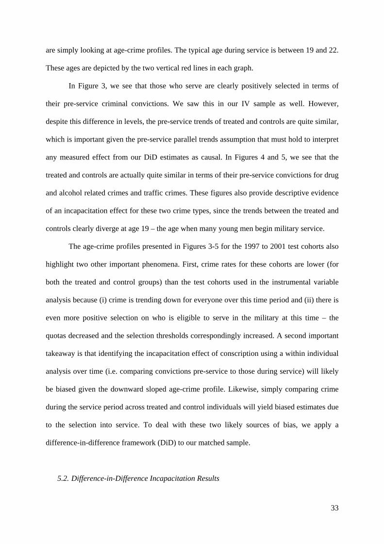
33

are simply looking at age-crime profiles. The typical age during service is between 19 and 22.

These ages are depicted by the two vertical red lines in each graph.

In Figure 3, we see that those who serve are clearly positively selected in terms of

their pre-service criminal convictions. We saw this in our IV sample as well. However,

despite this difference in levels, the pre-service trends of treated and controls are quite similar,

which is important given the pre-service parallel trends assumption that must hold to interpret

any measured effect from our DiD estimates as causal. In Figures 4 and 5, we see that the

treated and controls are actually quite similar in terms of their pre-service convictions for drug

and alcohol related crimes and traffic crimes. These figures also provide descriptive evidence

of an incapacitation effect for these two crime types, since the trends between the treated and

controls clearly diverge at age 19 – the age when many young men begin military service.

The age-crime profiles presented in Figures 3-5 for the 1997 to 2001 test cohorts also

highlight two other important phenomena. First, crime rates for these cohorts are lower (for

both the treated and control groups) than the test cohorts used in the instrumental variable

analysis because (i) crime is trending down for everyone over this time period and (ii) there is

even more positive selection on who is eligible to serve in the military at this time – the

quotas decreased and the selection thresholds correspondingly increased. A second important

takeaway is that identifying the incapacitation effect of conscription using a within individual

analysis over time (i.e. comparing convictions pre-service to those during service) will likely

be biased given the downward sloped age-crime profile. Likewise, simply comparing crime

during the service period across treated and control individuals will yield biased estimates due

to the selection into service. To deal with these two likely sources of bias, we apply a

difference-in-difference framework (DiD) to our matched sample.

5.2. Difference-in-Difference Incapacitation Results

34

For individual i in group ∈ , in period ∈ 1 _ , 2

, we estimate the following DiD regression equation:

(2) 2 ∗ 2 ,

where represents an individual fixed effect. The pre-service period is defined as the months

immediately preceding the start of military service, and is equal in length to the length of the

service period. For example, if a conscript serves 10 months in the military, then we search

his criminal record for any crimes committed during the ten months immediately preceding

his service period. Again, we assign this treated individual’s control counterpart the exact

same service and pre-service period, both equal to 10 months in this example. The

incapacitation effect of military service on crime is given by . Figures 2 – 4 provide

evidence in favor of the parallel trends assumption that allows us to interpret as causal.

Estimates of the incapacitation effect are shown in Table 12. As in our IV

incapacitation experiment (see Table 11), the estimated incapacitation effects for overall

crime at both margins are negative. At the extensive margin, the effect is driven by drug and

alcohol related crime. At the intensive margin, the effect is driven by both drug and alcohol

related crime and traffic crime. Interestingly, we find significant incapacitation effects for

both those with and without previous convictions. Taken together, our DiD and IV estimates

imply that there are significant incapacitation effects associated with military service.

5.3. Difference-in-Difference Post Service Results

For completeness, we also use our DiD framework to estimate the post-service effect in our

matched sample. We estimate an equation similar to Equation (2) after first redefining the two

35

time periods. The pre-service period is defined as crime committed between the ages of 15

and 17. The post-service period is crime committed between the ages of 23 and 30.

DiD estimates of the post service crime effect at the extensive margin are shown in

Panel A of Table 13. The post-service period intensive margin effects are shown in Appendix

Table 4. The estimated post-service effects for Any Crime, Weapons, Violent, Traffic, and

Other are all close to zero and insignificant. The coefficient associated with theft, however, is

positive, significant and large, with an effect size of 85%. However, we also see a significant

decrease in drug and alcohol related crime. In comparison, the OLS estimates presented in

Panel B of Table 13 all show large protective effects. These are clearly biased, despite the use

of a number of background control variables (including lagged crime) and test-day

information. We argue that our DiD goes a long way to remove these large biases.40

So, why are not all of the DiD estimates large and positive for cohorts tested between

1997 and 2001? First, crime in Sweden is trending down at the time when these men are in

their most crime prone years. Second, the experience of military service (i.e. the treatment) is

undergoing change. As fewer young men do service, then the more active they are kept doing

meaningful tasks. Also, the professional officer to conscript ratio rose. These and other

changes may have improved the experience of military service. Third, since the service rate is

falling substantially during this period, those who serve are more positively selected. That is,

the marginal conscripts in our DiD and IV exercises are not of the same quality. When the

effect of military service is heterogeneous (as we demonstrated above), and when service has

a more detrimental effect on those from low SES and/or high crime backgrounds, then as the

quality of the marginal conscript goes up, the detrimental effect should go down.

We illustrate this idea in Panel C of Table 13. Here, we show our extensive margin

DiD post-service effects broken down by quartiles of our estimated propensity score for

                                                            40 Because the difference-in-difference specification yields substantially different results for crime compared to OLS (with controls), we do not study the non-crime labor market outcomes for this matched sample, as there is no pre-period that we can define.

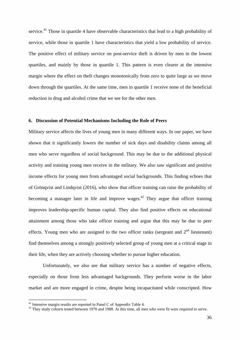
36

service.41 Those in quartile 4 have observable characteristics that lead to a high probability of

service, while those in quartile 1 have characteristics that yield a low probability of service.

The positive effect of military service on post-service theft is driven by men in the lowest

quartiles, and mainly by those in quartile 1. This pattern is even clearer at the intensive

margin where the effect on theft changes monotonically from zero to quite large as we move

down through the quartiles. At the same time, men in quartile 1 receive none of the beneficial

reduction in drug and alcohol crime that we see for the other men.

6. Discussion of Potential Mechanisms Including the Role of Peers

Military service affects the lives of young men in many different ways. In our paper, we have

shown that it significantly lowers the number of sick days and disability claims among all

men who serve regardless of social background. This may be due to the additional physical

activity and training young men receive in the military. We also saw significant and positive

income effects for young men from advantaged social backgrounds. This finding echoes that

of Grönqvist and Lindqvist (2016), who show that officer training can raise the probability of

becoming a manager later in life and improve wages.42 They argue that officer training

improves leadership-specific human capital. They also find positive effects on educational

attainment among those who take officer training and argue that this may be due to peer

effects. Young men who are assigned to the two officer ranks (sergeant and 2nd lieutenant)

find themselves among a strongly positively selected group of young men at a critical stage in

their life, when they are actively choosing whether to pursue higher education.

Unfortunately, we also see that military service has a number of negative effects,

especially on those from less advantaged backgrounds. They perform worse in the labor

market and are more engaged in crime, despite being incapacitated while conscripted. How

                                                            41 Intensive margin results are reported in Panel C of Appendix Table 4. 42 They study cohorts tested between 1970 and 1988. At this time, all men who were fit were required to serve.

37

does service generate such negative effects? Could negative peer influence be part of the

explanation?

To study this potential mechanism, we take our IV sample and group those who

actually serve into “units”. These are not the actual units (or platoons) in which they serve, as

we do not have access to data with platoon identifiers.43 Instead, our units are created by

grouping men by test year, regiment and rank. There are 114 regiments in our data and four

ranks – private, corporal, sergeant and 2nd lieutenant. We drop units with less than 10

members to allow for more accurate measures of average peer characteristics within a unit –

namely pre-service crime. The median unit size is 142; the mean is 162 and the maximum is

589. Although, these are not a conscript’s true platoon mates, this is the pool from which

platoon mates are drawn.

For each conscript, we then calculate the leave-out average pre-service crime rate of

all other men in his unit; that is, this average is based solely on the pre-service crime of each

young man’s peers, excluding himself. Figure 6 shows the distribution of the leave-out

average pre-service number of crimes across units, reported separately by rank. This figure

clearly shows that pre-service crime is concentrated among units of peers from the lowest

ranks. The entire distribution for privates, and to a lesser extent corporals, is markedly shifted

to the right. Men from low SES backgrounds tend also to be concentrated in these units; 29

percent of privates have fathers with nine or less years of schooling, compared to 19 percent

for corporals, and 12 percent for sergeants and 2nd lieutenants. Thus, one unintentional side-

effect of the recruitment and placement process is that high crime, low SES men are

concentrated together into smaller units, with intensive exposure over a long period of time.

But could this exposure then lead to peer effects in crime? In Table 14, we estimate

potential peer effects by regressing own post-service crime (at the ages 23-30) on the leave-

                                                            43 Platoons were typically comprised of 20 privates and corporals, one sergeant, and one 2nd lieutenant.

38

out mean pre-service crime rate in one’s unit. We control for birth month, birth year,

municipality, and test year by test office fixed effects, as well as the full set of test day and

pre-test day characteristics, including own pre-service crime. The first specification looks at

only the baseline relationship between peer criminal history and an individual’s post-service

crime. The remaining three columns interact peer criminal history with whether the individual

has a low educated father, has a criminal history themselves, and is a private or corporal,

respectively. Columns (1) – (4) present the extensive margin, while Columns (5) – (8) present

the intensive margin. The estimated peer effect for men from advantaged backgrounds (high

educated fathers or no criminal history) or with higher military ranks is zero; exposure to

peers with a criminal history does not increase post-service crime for individuals with a low

risk of crime to start with. In contrast, the results in Table 14 are indicative of strong peer

influences for individuals from disadvantaged backgrounds; increased exposure to peers with

a criminal history prior to service is associated with higher post-service crime for conscripts

assigned to lower military ranks, from lower SES households, and especially, with a criminal

history prior to service themselves. For example, having a criminal record prior to service

increases the likelihood of committing a crime post-service by almost nine percentage points;

evaluated at the mean, exposure to peers with a criminal history further increases the

likelihood of post service crime by an additional three percentage points. In this way, peer

effects appear to be reinforcing in nature – exposure to peers with a criminal history

reinforces the criminal path that individuals are already on.44 Such non-linear peer effects

imply that how conscripts are allocated to a unit can affect post-service crime. Thus, one way

                                                            44 This is consistent with the findings of reinforcing peer effects in juvenile correctional facilities by Bayer, Hjalmarsson, and Pozen (2009), though those were crime-specific in nature.

39

to limit the potential negative (unintended) effects of military service may be to not group all

“bad apples” together.45

Taken together, the concentration of high crime men into the same units of service and

potential strong peer effects make negative peer effects one plausible mechanism behind the

negative effects that we find for low SES men. Quantifying this effect, however, is quite

difficult, since we lack a well-defined measure of the counterfactual peer groups that these

young men would have faced if they had not been placed in service. Not only is the

composition of the counterfactual peer group difficult to identify, but also the intensity of

exposure – military service not only changes the composition of peers but also the intensity of

the peer interactions. In this way, even if the average peer characteristics are not that different,

peer effects of service could be quite strong since the nature of the interactions has changed.

Of course, there are other potential mechanisms that could also be at work. In

particular, we would like to point out the fact that our cohorts of men were leaving service

and entering into an environment with rather high unemployment among young adults. One

conjecture is that among low skilled workers, those who do not undertake military service are

able to establish themselves on the labor market more quickly. As we saw in Table 10, the

marginal conscript experiences more unemployment as a young adult.

Finally, it has been suggested that a desensitization to violence and weapons can

exacerbate post-service crime. In an attempt to get at this potential channel, we classify

individuals’ service categories as combatant (e.g. infantry soldier) versus noncombatant (e.g.

cook). For the sample that serves, we then run OLS regressions of post-service crime on

combatant status, with and without the full set of observable controls.46 In the raw data, we

find that individuals who serve in combat positions are less likely to commit post-service

                                                            45 However, as demonstrated by Carrell, Sacerdote, and West (2013), caution should be exercised when trying to optimally design peer groups based on reduced form peer effects. They in fact found perverse effects of the ‘optimal’ assignments to squadrons in the United States Airforce Academy. 46 Available from the authors upon request.

40

crime; with the full set of observable controls, there are no significant differences in post-

service crime rates. One clearly cannot assign a causal interpretation to these results, as

service category is not randomly assigned; however, given these findings, it is hard to believe

that desensitization to violence (via combat training) is the mechanism underlying the large

effect of service on post-service crime.47

7. Conclusion

With the end of the Cold War, numerous countries in Europe abolished mandatory

conscription. With no imminent military threat, and with the security of NATO or EU

membership, it became hard for politicians to both justify the financial costs of such a large-

scale national policy and to convince voters of the need for it on civic grounds alone (Bieri,

2015). In recent years, the debate has about-faced, with many countries considering a re-

instatement of mandatory conscription in some form. Perhaps not surprisingly, with the

annexation of Crimea by Russia, both Lithuania and the Ukraine have already reinstated the

draft. However, this conversation is also happening in countries in Western Europe – namely

France, Italy, the UK and Sweden (Bieri, 2015). While one should clearly debate these issues

with respect to the direct costs and the likely need for and competence of such a military, one

must also consider the potential indirect costs associated with mandatory conscription.

Using an instrumental variable approach that takes advantage of exogenous variation

in the likelihood of service due to randomly assigned draft board officiators, we show that the

potential indirect costs of mandatory conscription may indeed be high. Despite providing the

first evidence that individuals are incapacitated from committing crimes while conscripted (in

both the IV design and difference in difference analysis), we find that conscription increases

post-service crimes from ages 23 to 30 at both the extensive and intensive margins and across

                                                            47 Note that we cannot use our IV specifications on combat and noncombat samples; first stage f-statistics are not large enough to justify such a specification.

41

a number of crime categories, including violent crimes and thefts. Thus, any long term crime

reducing effects of incapacitation are more than offset by other ways in which the military

negatively affects crime. In addition, these detrimental effects of service are driven by

relatively ‘high risk’ populations with respect to future crime (i.e. those with a criminal

history prior to service and/or from low socioeconomic status backgrounds). We provide

evidence that grouping high crime, low SES individuals together in an environment with high

intensity peer exposure may be one feasible explanation for the negative effects of service for

these high risk populations – i.e. reinforcing peer effects. We find little evidence in support of

a desensitization to weapons and violence channel, but cannot rule out a weaker labor market

attachment as an explanation of the results. Unfortunately, regardless of the mechanism, these

results contradict the idea that military service may be a way to straighten out troubled youths

and build skills that are marketable in the post-service labor market.

On a brighter note, we find that mandatory conscription improves the health of all

young men and can have other positive post-service effects for populations at low-risk for

crime. In the instrumental variable analysis, there is no post-service effect on crime and there

are actually improved labor market outcomes for individuals from non-criminal backgrounds

and better educated families. In addition, our supplementary difference-in-difference

matching analysis suggests that service can lead to a long lasting reduction of drug and

alcohol related crime. But, this is for a positively selected sample, with low crime rates to start

with. Even in this sample, however, there is still evidence of a detrimental effect of service on

post-service crime (mainly property crime) when zooming in on the lower end of the

distribution.

Taken together, the results of our analysis indicate mandatory military conscription

does have a significant impact on the life course of young men, and that this impact is quite

heterogeneous, such that it may reinforce already existing inequalities in the likelihood of

42

future success. These non-monetary costs (and/or benefits) should be taken into account when

deciding whether to reinstate or abolish mandatory conscription or when devising the system

through which conscription occurs (e.g. lottery, testing, etc.). Who are the average and

marginal conscripts? How will conscription affect these individuals?

43

References Aizer, Anna and Joe Doyle (2015) “Juvenile Incarceration, Human Capital and Future Crime: Evidence from Randomly-assigned Judges,” Quarterly Journal of Economics 130(2), 759-803. Albaek, Karsten, SØren Leth-Petersen, Daniel le Maire and Torben Tranaes (forthcoming) “Does Peacetime Military Service Affect Crime?” Scandinavian Journal of Economics. Albrecht, James W., Per-Anders Edin, Marianne Sundström and Susan B. Vroman (1999) “Career Interruptions and Subsequent Earnings: A Reexamination Using Swedish Data,” Journal of Human Resources 34(2), 294-311.

Anderson, D. Mark and Daniel Rees (2015) “Deployments, Combat Exposure, and Crime,” Journal of Law and Economics 58, 235-267. Angrist, Joshua D. (1990) “Lifetime Earnings and the Vietnam Era Draft Lottery: Evidence from Social Security Administrative Records," American Economic Review 80(3), 313-336. Angrist, Joshua D. and Stacey H. Chen (2011) “Schooling and the Vietnam Era GI Bill: Evidence from the Draft Lottery,” American Economic Journal: Applied Economics 3(2), 96-118. Angrist, Joshua D., Stacey H. Chen and Brigham R. Frandsen (2010) “Did Vietnam Veterans Get Sicker in the 1990s? The Complicated Effects of Military Service on Self-Reported Health,” The Journal of Public Economics 94(11-12), 824-837. Angrist, Joshua D., Stacey H. Chen and Jae Song (2011) “Long-term Consequences of Vietnam-Era Conscription: New Estimates Using Social Security Data,” American Economic Review: Papers and Proceedings 101(3), 334–338. Autor, David, Mark Duggan and David Lyle (2011) "Battle Scars: the Puzzling Decline in Employment and Rise in Disability Receipt among Vietnam-Era Veterans," American Economic Review: Papers and Proceedings 101(3), 339-349. Bayer, Patrick, Randi Hjalmarsson and David Pozen (2009) “Building Criminal Capital Behind Bars: Peer Effects in Juvenile Corrections,” Quarterly Journal of Economics 124(1), 105-147. Becker, Gary (1968) “Crime and Punishment: An Economic Approach,” The Journal of Political Economy 76(2), 169-217.

Beckerman, Adela and Leonard Fontana (1989) “Vietnam Veterans and the Criminal Justice System: A Selected Review,” Criminal Justice and Behavior 16 (4), 412-428. Bedard, Kelly and Olivier Deschênes (2006) “The Long-Term Impact of Military Service on Health Outcomes: Evidence from World War II and Korean War Veterans,” The American Economic Review 96(1), 176-194.

44

Bieri, Matthias (2015) “Military Conscription in Europe: New Relevance,” CSS Analyses in Security Policy, Center for Security Studies, ETH Zurich. Bingley, Paul, Petter Lundborg and Stéphanie Vincent Lyk-Jensen (2014) “Opportunity Cost and the Incidence of a Draft Lottery,” IZA DP No. 8057. Böhlmark, Anders and Matthew J. Lindquist (2006) “Life-Cycle Variations in the Association between Current and Lifetime Income: Replication and Extension for Sweden,” Journal of Labor Economics 24(4), 879-896. Card, David and Ana Rute Cardoso (2012) “Can Compulsory Military Service Raise Civilian Wages? Evidence from the Peacetime Draft in Portugal,” American Economic Journal: Applied Economics 4(4), 57-93. Carlsson, Magnus, Gordon Dahl, Björn Öckert and Dan-Olof Rooth (2015) “The Effect of Schooling on Cognitive Skills,” Review of Economics and Statistics 97 (3), 533-547. Dobkin, Carlos and Reza Shabani (2009). “The Health Effects of Military Service: Evidence from the Vietnam Draft,” Economic Inquiry 47(1), 69-80. Carrell, Scott, Bruce Sacerdote and James West (2013) “From Natural Variation to Optimal Policy? The Importance of Endogenous Peer Group Formation,” Econometrica 81(3), 855-882. Doyle Jr., Joseph J. (2008) “Child Protection and Adult Crime: Using Investigator Assignment to Estimate Causal Effects of Foster Care,” Journal of Political Economy 116(4), 746-770.

Galiani, Sebastian, Martín A. Rossi, and E. Schargrodsky (2011): “The Effects of Peacetime and Wartime Conscription on Criminal Activity," American Economic Journal: Applied Economics 3(2), 119-136. Grenet, J., R. Hart, and Ernesto Roberts (2011) “Above and Beyond the Call: Long-term Real Earnings Effects of British Male Military Conscription in the Post-War Years,” Labour Economics 18(2), 194-204. Grossman, Dave (1995) On Killing. The Psychological Cost of Learning to Kill in War and Society (Boston: Little, Brown).

Grönqvist, Erik and Erik Lindqvist (2016) “The Making of a Manager: Evidence from Military Officer Training,” Journal of Labor Economics 34(4).

Hanes, Niklas, Erik Norlin and Magnus Sjöström (2010) “The Civil Returns of Military Training: A Study of Young Men in Sweden,” Defense and Peace Economics 21(5), 547-565.

Jacob, Brian and Lars Lefgren (2003) “Are Idle Hands the Devil's Workshop? Incapacitation, Concentration, and Juvenile Crime,” American Economic Review 93(5), 1560-1577.

45

Johnston David W., Michael A. Shield, Peter Siminski (forthcoming) “Long-Term Health Effects of Vietnam-Era Military Service: A Quasi-Experiment using Australian Conscription Lotteries,” Journal of Health Economics.

Kling, Jeffrey (2006) “Incarceration Length, Employment, and Earnings,” American Economic Review 96(3), 863-876. Lindo, Jason M. and Charles Stoecker (2014) “Drawn into Violence: Evidence on ‘What Makes a Criminal’ from the Vietnam Draft Lotteries,” Economic Inquiry 52(1), 239-258.

Luallen, Jeremy (2006) “School's Out...Forever: A Study of Juvenile Crime, At-Risk Youths and Teacher Strikes,” Journal of Urban Economics 59(1), 75-103.

Maurin, Eric and Theodora Xenogiani (2007) “Demand for Education and Labor Market Outcomes. Lessons from the Abolition of Compulsory Conscription in France,” Journal of Human Resources 42(4), 795-819. Mueller-Smith, Michael (2015) “The Criminal and Labor Market Impacts of Incarceration,” unpublished manuscript, University of Michigan. Resnick, Heidi S., David W. Foy, Clyde P. Donahoe and Eric N. Miller (1989) “Antisocial Behavior and Post-traumatic Stress Disorder in Vietnam Veterans,” Journal of Clinical Psychology 45(6), 860-866. Rohlfs, Chris (2010) “Does combat exposure make you a more violent or criminal person? Evidence from the Vietnam draft,” Journal of Human Resources 45(2), 271-300. Siminski, Peter (2013) “Employment Effects of Army Service and Veterans Compensation: Evidence from the Australian Vietnam-Era Conscription Lotteries,” Review of Economics and Statistics 95(1), 87-97. Siminski, Peter, Simon Ville, and Alexander Paull (2016). “Does the Military Train Men to Be Violent Criminals? New Evidence from Australia’s Conscription Lotteries,” Journal of Population Economics 29(1), 197-218.

Yesavage, Jerome (1983) “Differential Effects of Vietnam Combat Experiences vs Criminality on Dangerous Behavior by Vietnam Veterans with Schizophrenia,” The Journal of Nervous and Mental Disease 171(6), 382-384.

46

Figure 1. Share of Sweden born Males Who Were Tested, Share Assigned to a Service Category, and Share Who Served in the Military by Birth Cohort.

 

New Draft Authority ->

Internet Based Pre-Test

0.1

.2.3

.4.5

.6.7

.8.9

1

1965 1970 1975 1980 1985 1990year of birth

share tested share assigned service categoryshare served in military

Sweden born males

47

Figure 2. Share Serve from 1990 to 1996 Test Cohorts

Note – This graph is based on the sample used in the instrumental variable analysis. That is, it is the share that serve of the sample of non-immigrant males who tested in 1990 to 1996 and were eligible to serve. For more details on the sample criteria, see Appendix Table 1.

.9.8

5.8

.75

.7.6

5.6

.55

.5sh

are

se

rve

1990 1992 1994 1996test year

y p

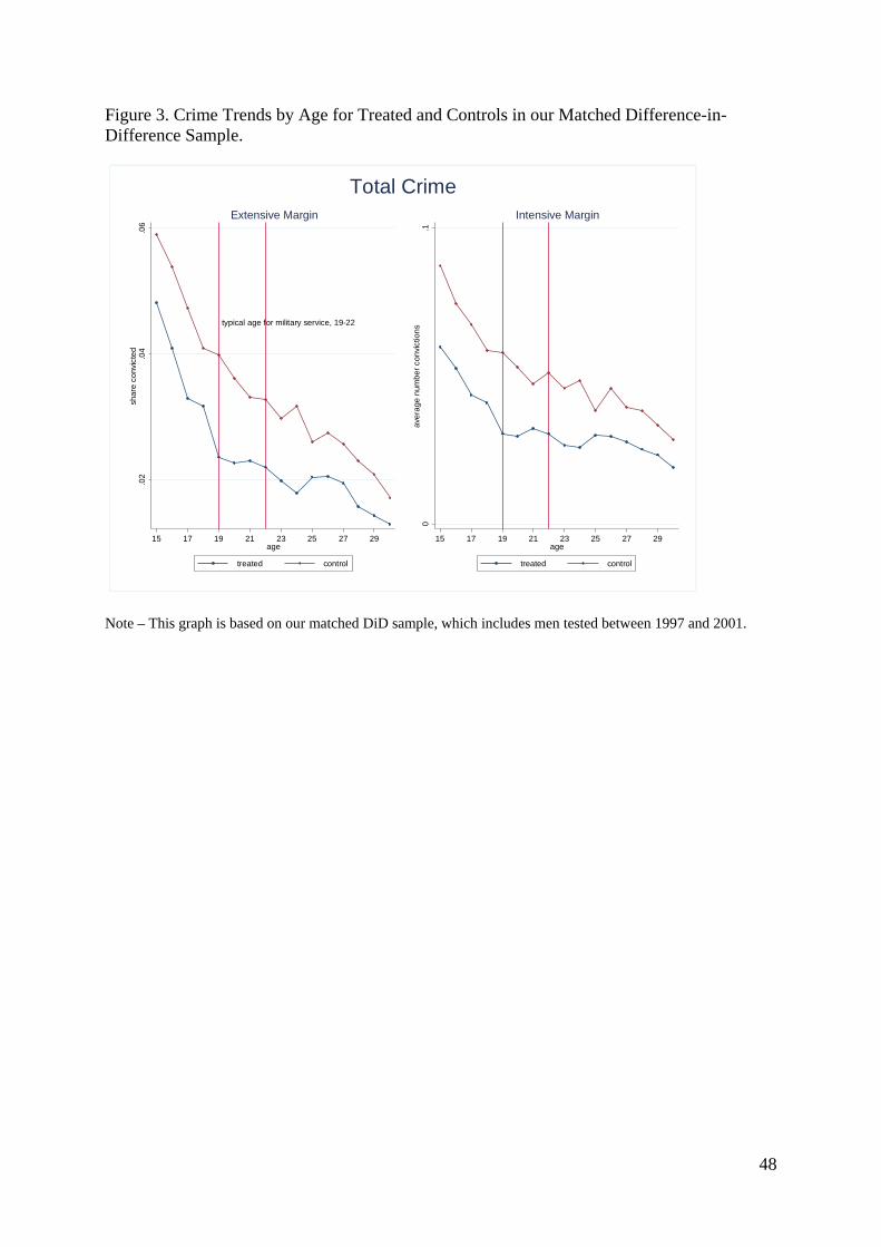
48

Figure 3. Crime Trends by Age for Treated and Controls in our Matched Difference-in-Difference Sample.

Note – This graph is based on our matched DiD sample, which includes men tested between 1997 and 2001.

   

typical age for military service, 19-22

.02

.04

.06

sha

re c

onv

icte

d

15 17 19 21 23 25 27 29age

treated control

Extensive Margin

0.1

ave

rag

e n

um

ber

co

nvi

ctio

ns

15 17 19 21 23 25 27 29age

treated control

Intensive Margin

Total Crime

49

Figure 4. Trends in Crime Type by Age for Treated and Controls in our Matched Difference-in-Difference Sample, Extensive Margin.

Note – This graph is based on our matched DiD sample, which includes men tested between 1997 and 2001.

typical age for militaryservice, 19-22

0.0

1.0

2sh

are

co

nvic

ted

15 17 19 21 23 25 27 29age

treated control

Theft

0.0

1

15 17 19 21 23 25 27 29age

treated control

Violent

0.0

01

.00

2

15 17 19 21 23 25 27 29age

treated control

Weapons

0.0

1sh

are

co

nvic

ted

15 17 19 21 23 25 27 29age

treated control

Drugs & Alcohol

.00

5.0

1.0

15

15 17 19 21 23 25 27 29age

treated control

Traffic

0.0

05

.01

15 17 19 21 23 25 27 29age

treated control

Other

Extensive Margin Variables

50

Figure 5. Trends in Crime Type by Age for Treated and Controls in our Matched Difference-in-Difference Sample, Intensive Margin.

Note – This graph is based on our matched DiD sample, which includes men tested between 1997 and 2001.

typical age for military

service, 19-22

0.0

2.0

4a

vera

ge

nu

mb

er c

on

vict

ion

s

15 17 19 21 23 25 27 29age

treated control

Theft

0.0

2

15 17 19 21 23 25 27 29age

treated control

Violent

0.0

02.0

04

15 17 19 21 23 25 27 29age

treated control

Weapons

0.0

05

.01

ave

rag

e n

um

ber

co

nvi

ctio

ns

15 17 19 21 23 25 27 29age

treated control

Drugs & Alcohol

.01

.01

5.0

2

15 17 19 21 23 25 27 29age

treated control

Traffic

0.0

2

15 17 19 21 23 25 27 29age

treated control

Other

Intensive Margin Variables

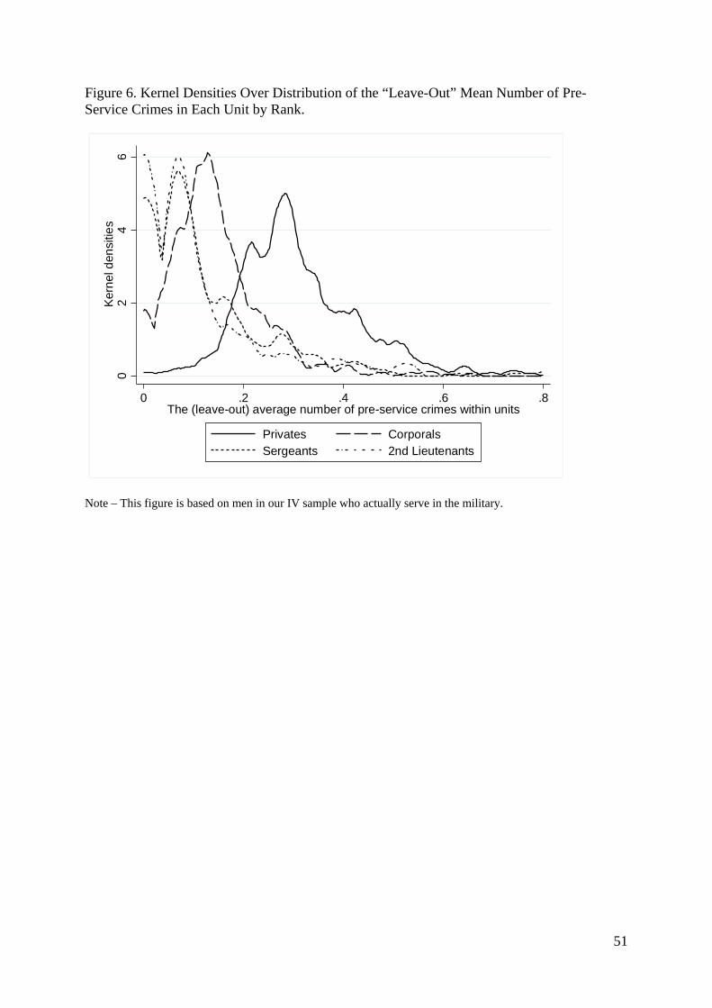
51

Figure 6. Kernel Densities Over Distribution of the “Leave-Out” Mean Number of Pre-Service Crimes in Each Unit by Rank.

Note – This figure is based on men in our IV sample who actually serve in the military.

02

46

Ker

nel

den

sitie

s

0 .2 .4 .6 .8The (leave-out) average number of pre-service crimes within units

Privates CorporalsSergeants 2nd Lieutenants

52

Table 1. Summary Statistics: Overall and By Service

All Individuals (N = 168,818)

Service = 1 (N = 126,550)

Service = 0 (N = 42,268)

Variable Mean SD Mean SD Mean SD military service (tax records) 0.75 0.43 1.00 0.00 0.00 0.00 high service rate officiator 0.50 0.50 0.56 0.50 0.35 0.48 test_year 1992.76 1.98 1992.71 1.96 1992.88 2.03 birth_year 1974.56 2.03 1974.55 2.01 1974.62 2.07

Pre-test day controls Any crime < 18? 0.13 0.34 0.13 0.34 0.15 0.35 schooling father 11.14 2.65 11.16 2.63 11.08 2.73 schooling mother 11.55 2.35 11.57 2.32 11.49 2.42 income father 12.32 0.40 12.32 0.40 12.30 0.41 income mother 11.87 0.39 11.87 0.38 11.85 0.40 2 year school? 0.18 0.39 0.18 0.38 0.19 0.39 3 year school? 0.76 0.43 0.77 0.42 0.72 0.45

Test Day Controls Height 179.75 6.44 179.77 6.41 179.66 6.50 Weight 71.59 10.53 71.65 10.48 71.40 10.67 Bmi 22.14 2.89 22.15 2.88 22.10 2.93 Ability Score 5.17 1.84 5.22 1.80 5.05 1.94 Physical Capacity Score 6.26 1.45 6.35 1.43 5.98 1.48

Crime Outcomes Any crimes 23-30? 0.10 0.31 0.10 0.30 0.11 0.32 # crimes 23-30 0.31 2.33 0.28 2.10 0.40 2.91 Any weapons 23-30 0.01 0.07 0.01 0.07 0.01 0.08 Any violent 23-30 0.02 0.15 0.02 0.15 0.03 0.16 Any traffic 23-30 0.06 0.25 0.06 0.24 0.07 0.25 Any theft 23-30 0.01 0.11 0.01 0.11 0.02 0.13 Any other 23-30 0.02 0.15 0.02 0.15 0.03 0.17 Any drugs 23-30 0.02 0.13 0.01 0.12 0.02 0.14 # weapons 23-30 0.01 0.21 0.01 0.17 0.01 0.30 # violent 23-30 0.05 0.44 0.04 0.41 0.06 0.52 # traffic 23-30 0.13 1.00 0.12 0.90 0.16 1.25 # theft 23-30 0.04 0.60 0.03 0.55 0.05 0.74 # other 23-30 0.05 0.44 0.04 0.42 0.06 0.52 # drugs 23-30 0.05 0.59 0.04 0.55 0.06 0.70 Note - Missing observations are replaced with sample means (for the control variables only).

53

Table 2. Raw Comparison of Pre-Characteristics Across High Service Rate Officiator Assignment

High Service Rate Officiator = 1

(N=85,138) High Service Rate Officiator =0

(N=83,668) Variable Mean Std. Mean Std. Difference % Difference military service 0.83 0.38 0.67 0.47 0.16 18.8 test_year 1993.04 2.03 1992.47 1.88 0.56 0.0 birth_year 1974.86 2.10 1974.27 1.91 0.59 0.0 any crime < 18 0.14 0.34 0.13 0.34 0.01 4.9 schooling father 11.33 2.64 10.95 2.65 0.38 3.4 schooling mother 11.71 2.33 11.38 2.35 0.32 2.7 income father 12.33 0.42 12.30 0.38 0.03 0.3 income mother 11.90 0.39 11.83 0.38 0.07 0.6 2 year shcool? 0.16 0.37 0.20 0.40 -0.04 -22.4 3 year school? 0.77 0.42 0.74 0.44 0.03 4.5 height 179.74 6.43 179.75 6.44 -0.01 0.0 weight 71.55 10.49 71.63 10.56 -0.08 -0.1 bmi 22.13 2.88 22.15 2.90 -0.02 -0.1 ability score 5.22 1.83 5.13 1.85 0.09 1.7 physical capacity score 6.29 1.36 6.22 1.53 0.08 1.2

54

Table 3. Test of Random Assignment to Officiators

(1) (2) (3) (4) (5) (6) (7)

Dependent Variable: High Service Rate Officiator Unexplained High Service

# (of 21) significant 5% (including missing dummies) 9 4 3 2 4 4 0 # (of 12) significant 5% (excluding missing dummies) 4 3 2 2 4 4 0

pvalue prechar (variables) 0 0.05 0.15 0.12 0.17 0.18 0.85 pvalue test day char (variables) 0.13 0.01 0.04 0.02 0.03 0.04 0.22 pvalue pre and test day char (variables) 0 0.12 0.12 0.1 0.12 0.15 0.37 county FE no Yes yes yes yes yes no test year FE no No yes yes yes yes no county x test year FE no No no yes yes yes no test office FE no No no no yes yes no test office x test year FE no No no no no yes no PreCharacteristics any crime < 18 0.02468*** 0.00657* 0.00251 0.00227 0.00209 0.00203 0.00229

[0.00814] [0.00389] [0.00262] [0.00245] [0.00249] [0.00248] [0.00314] schooling father 0.00812*** 0.00044* -0.00039 0.00008 0.00006 0.00008 0.00009

[0.00125] [0.00025] [0.00027] [0.00020] [0.00019] [0.00019] [0.00050] schooling mother 0.00330*** 0.00218*** 0.00053 -0.00001 -0.00003 -0.00003 -0.00001

[0.00117] [0.00067] [0.00040] [0.00034] [0.00033] [0.00033] [0.00047] income father 0.00226 -0.00979*** -0.00118 -0.00244 -0.00207 -0.00215 -0.00235

[0.01944] [0.00350] [0.00182] [0.00158] [0.00163] [0.00161] [0.00458] income mother 0.09168*** 0.00272 -0.00024 0.00171 0.00136 0.00142 0.00178

[0.01633] [0.00216] [0.00201] [0.00150] [0.00149] [0.00149] [0.00415] 2 year school? -0.05682* -0.04488*** 0.00919** 0.00422* 0.00457** 0.00418** 0.00404

[0.03109] [0.01374] [0.00363] [0.00225] [0.00214] [0.00203] [0.01103] 3 year school? -0.01375 0.01969* 0.01340*** 0.00523* 0.00579** 0.00562** 0.00518

[0.02486] [0.01090] [0.00476] [0.00267] [0.00252] [0.00248] [0.00959] Test Day Characteristics height -0.00017 -0.00016 -0.00042 -0.00093 -0.00097 -0.00105 -0.00091

55

[0.00219] [0.00075] [0.00077] [0.00077] [0.00075] [0.00076] [0.00089] weight -0.00056 0.00019 0.00069 0.00123 0.00129 0.0014 0.00122

[0.00256] [0.00094] [0.00098] [0.00095] [0.00093] [0.00094] [0.00110] bmi 0.00265 0.00071 -0.00216 -0.00438 -0.00452 -0.00486 -0.00434

[0.00768] [0.00334] [0.00329] [0.00313] [0.00308] [0.00309] [0.00355] ability score -0.00379 -0.00434*** -0.00173* -0.00127** -0.00132** -0.00129** -0.00127

[0.00255] [0.00127] [0.00097] [0.00057] [0.00055] [0.00054] [0.00106] physical capacity 0.0053 -0.00084 0.00337* 0.00148*** 0.00144** 0.00138** 0.0014

[0.00906] [0.00208] [0.00187] [0.00056] [0.00054] [0.00056] [0.00299]

Observations 168806 168806 168806 168806 168806 168806 168806 R-squared 0.01 0.62 0.66 0.75 0.75 0.75 0

Robust standard errors (clustered at officiator)

The dependent variable in column (7) is the residual from a regression of assignment to a high service rate officiator on test year * county fixed effects, i.e. the variation in officiator assignment not explained by geographical and test year fixed effects.

56

Table 4. First Stage Regressions of Military Service on Assignment to High Service Rate Officiator

(1) (2) (3) (4) (5) (6) (7) (8) Dependent Variable = military_service_tax_record

High Service Rate Officiator 0.15513*** 0.06859*** 0.10229*** 0.07933*** 0.07780*** 0.07713*** 0.07686*** 0.07596*** [0.01999] [0.00931] [0.01166] [0.01398] [0.01387] [0.01405] [0.01403] [0.01385]

F-statistic 60 54 77 32 31 30 30 30

county FE no yes yes yes yes yes yes yes test year FE no no yes yes yes yes yes yes county x test year FE no no no yes yes yes yes yes test office FE no no no no yes yes yes yes test office x test year FE no no no no no yes yes yes pretest day characteristic no no no no no no yes yes test day variables no no no no no no no yes Observations 168806 168806 168806 168806 168806 168806 168806 168806 R-squared 0.03 0.05 0.06 0.07 0.07 0.07 0.07 0.08

Robust standard errors, clustered by officiator. *** significant at 1%, ** significant at 5%, * significant at 10%

57

Table 5. Baseline OLS and IV Estimates for Overall Crime

(1) (2) (3) (4) (5) OLS OLS OLS IV IV Panel A: Dependent Variable = Any Crimes from Age 23-30 (Mean = 0.10) military_service -0.01233*** -0.01661*** -0.00663*** 0.08908* 0.08072*

[0.00283] [0.00277] [0.00220] [0.04779] [0.04478]

Panel B: Dependent Variable = # Crimes from Age 23-30 (Mean = 0.31) military_service -0.12176*** -0.13289*** -0.06648*** 0.55856** 0.54746**

[0.01775] [0.01965] [0.01682] [0.25192] [0.22346]

First Stage F-Statistic 32 31 county x test year fixed effects no yes yes yes yes Test office Fixed Effects no no yes no yes Pre-test and Test day Controls no no yes no yes Columns (1) – (3) present the results of regressing crime from 23-30 (at the extensive margin in Panel A and the intensive margin in Panel B) on military service and the indicated set of controls. Note that county x test year fixed effects implies the inclusion of county dummies, test year dummies, and county by test year dummies. For the ease of presentation, just the coefficient on military service is reported. Columns (4) and (5) instrument for military service with assignment to a high service rate officiator. Robust standard errors, clustered by county in columns (1) - (3) and officiator in columns (4)-(5). *** significant 1%, ** significant 5%, * significant 10%. N= 168806

58

Table 6. Instrumental Variable Estimates of the Effect of Service on Post-Conscription Crime, by Crime Type

Dependent Variable: (1) (2) (3) (4) (5) (6) (7)

Any Crime Weapons Violent Traffic Theft Other Drugs/Alc extensive margin 23-30 Baseline 0.08908* 0.01650** 0.04934*** 0.02943 0.01967 0.01886 0.01664

[0.04779] [0.00823] [0.01609] [0.03362] [0.01322] [0.02053] [0.01527]

+ <18 crime specific control 0.08053* 0.01597* 0.04881*** 0.02308 0.01898 0.02019 0.01566

+ test office, pre testday and test day controls 0.08072* 0.01550* 0.04691*** 0.02309 0.01876 0.01959 0.01463

Mean Dependent Variable 0.10 0.006 0.023 0.064 0.013 0.025 0.016 intensive margin 23-30 Baseline 0.55856** 0.01272 0.10193** 0.05209 0.17040*** 0.10175* 0.11969**

[0.25192] [0.02072] [0.04728] [0.15086] [0.05596] [0.05626] [0.05645]

+ <18 crime specific control 0.50565** 0.01135 0.10050** 0.02744 0.16752*** 0.10542* 0.11429**

+ test office, pre testday and test day controls 0.51767** 0.00879 0.08812* 0.05188 0.15907*** 0.11326** 0.11413**

Mean Dependent Variable 0.31 0.01 0.046 0.13 0.038 0.046 0.047

Robust standard errors, clustered on officiator. *** 1%, ** 5%, * 10*. N = 168,806. The baseline regressions control just for test year dummies, county dummies and test year x county dummies, and is equivalent to the specification presented in column (4) of Table 5. These controls are also included in all other regressions. All specifications instrument for military service with assignment to a high service rate officiator. Just the coefficient on military service is presented. For the baseline specifications, the first stage F-statistic is 32. It remains at 32 when controlling for having at least one conviction in the crime category that corresponds to the dependent variable, and is equal to 31 when adding the full set of controls.

59

Table 7. Falsification Test: Military Service and Pre-Service Crime

Dependent Variable: (1) (2) (3) (4) (5) (6) (7)

Any Crime Weapons Violent Traffic Theft Other Drugs/Alc extensive margin: convictions less than age 18 Military Service 0.05208 0.00829 0.00352 0.05467 0.0111 -0.01838 0.0069

[0.05100] [0.00880] [0.01421] [0.03343] [0.02463] [0.02462] [0.00603]

Mean Dependent Variable 0.13 0.006 0.019 0.055 0.059 0.038 0.004 intensive margin: convictions less than age 18 Military Service 0.23332 0.01465 0.007 0.03298 0.18977 -0.02942 0.01834

[0.20724] [0.01850] [0.03701] [0.04871] [0.12263] [0.05111] [0.01159]

Mean Dependent Variable 0.32 0.013 0.028 0.078 0.13 0.059 0.005

Robust standard errors, clustered on officiator. *** 1%, ** 5%, * 10*. N = 168,806 (corresponding to 1990-1996 test years). Presents the results for estimating the baseline regression (test year dummies, county dummies and test year x county dummies). The dependent variable is having at least one conviction or the number of convictions in the crime category listed at the top of column prior to age 18, i.e. before military service. All specifications instrument for military service with assignment to a high service rate officiator. Just the coefficient on military service is presented. The first stage F-statistic is 32.

60

Table 8. IV Estimates of Post-Service Crime Effect: Heterogeneity by Criminal History

Dependent Variable: Any Crime Weapons Violent Traffic Theft Other Drugs/Alc Panel A: extensive margin from age 23 to 30 Sample: At least one crime < 18 (n = 22590) 0.22203** 0.08171 0.10332* 0.09591 0.12952** 0.09816 0.07183

[0.10382] [0.05014] [0.05762] [0.07425] [0.06512] [0.08492] [0.06502] Mean Dep Variable 0.24 0.023 0.072 0.15 0.048 0.071 0.06

Sample: No crimes < 18 (n=146216) 0.05617 0.00243 0.03660** 0.0135 -0.00372 0.00058 0.00336 [0.03987] [0.00656] [0.01497] [0.03232] [0.01220] [0.01522] [0.01111]

Mean Dep Variable 0.082 0.008 0.015 0.052 0.008 0.017 0.009 Panel B: intensive margin from Age 23 to 30 Sample: At least one crime < 18 (n = 22590) 2.79733* 0.10884 0.41801* 0.62365 0.77635** 0.28647 0.58402**

[1.46966] [0.12904] [0.22971] [0.71503] [0.38001] [0.23522] [0.28557] Mean Dep Variable 1.18 0.047 0.17 0.42 0.17 0.16 0.21

Sample: No crimes < 18 (n=146216) 0.0344 -0.0099 0.0292 -0.08491 0.03978 0.05128 0.00896 [0.17234] [0.01456] [0.03219] [0.08382] [0.03790] [0.04293] [0.04037]

Mean Dep Variable 0.18 0.004 0.026 0.08 0.017 0.028 0.021 Robust standard errors, clustered on officiator. *** 1%, ** 5%, * 10*. Military Service is instrumented for with the high service rate officiator dummy. F-statistic on first stage regressions: 27 for sample with criminal history and 30 for sample without criminal history. Each regression controls for test year dummies, county dummies and test year x county dummies.

61

Table 9. IV Estimates of Post-Service Crime Effect: Heterogeneity by Father Schooling

Dependent Variable: Any Crime Weapons Violent Traffic Theft Other Drugs/Alc Panel A: extensive margin from age 23 to 30 Father School <= 9 years (N = 43904) 0.10682* 0.02667* 0.08606** 0.02519 0.04018 0.03325 0.05055**

[0.06044] [0.01458] [0.03580] [0.04161] [0.02724] [0.03382] [0.02493]

Father School > 9 & <= 12 years (N=90346) 0.07447 0.01188 0.03778 0.01162 0.00817 0.03095 -0.00138

[0.05435] [0.01345] [0.02400] [0.03915] [0.01797] [0.02803] [0.02323]

Father School > 12 years (n = 34466) 0.10481 0.01014 0.01864 0.08786 0.01251 -0.03635 0.00603 [0.08351] [0.01164] [0.03059] [0.06685] [0.01802] [0.02762] [0.02115]

Panel B: intensive margin from Age 23 to 30 Father School <= 9 years (N = 43904) 1.12559** 0.04135 0.14591 0.39832 0.26554** 0.08606 0.18841**

[0.44410] [0.04246] [0.09486] [0.28446] [0.11226] [0.08601] [0.09039]

Father School > 9 & <= 12 years (N=90346) 0.3969 -0.00344 0.10325 -0.13782 0.18118** 0.13810* 0.11564

[0.35510] [0.03283] [0.07445] [0.19729] [0.08263] [0.08049] [0.09713]

Father School > 12 years (n = 34466) -0.00161 0.00259 0.01807 -0.04469 -0.01394 0.03356 0.0028 [0.23377] [0.01924] [0.06835] [0.10082] [0.03610] [0.07399] [0.07810]

Robust standard errors, clustered on officiator. *** 1%, ** 5%, * 10*. Military Service is instrumented for with the high service rate officiator dummy. F-statistic on first stage regressions: 40.6 for father school <=9, 24 for father schooling >9 and <=12, 22 for father shcooling > 12. Each regression controls for test year dummies, county dummies and test year x county dummies.

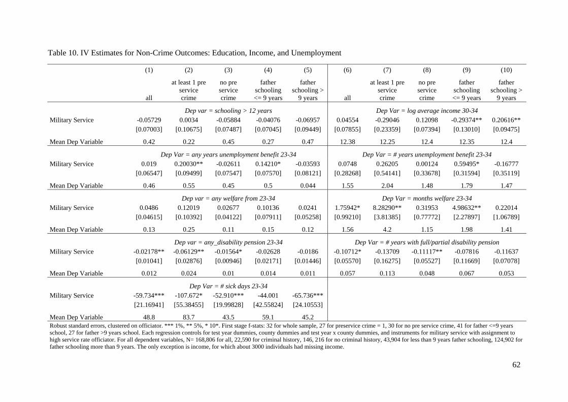
62

Table 10. IV Estimates for Non-Crime Outcomes: Education, Income, and Unemployment

(1) (2) (3) (4) (5) (6) (7) (8) (9) (10)

all

at least 1 pre service crime

no pre service crime

father schooling <= 9 years

father schooling >

9 years all

at least 1 pre service crime

no pre service crime

father schooling <= 9 years

father schooling >

9 years

Dep var = schooling > 12 years Dep Var = log average income 30-34 Military Service -0.05729 0.0034 -0.05884 -0.04076 -0.06957 0.04554 -0.29046 0.12098 -0.29374** 0.20616**

[0.07003] [0.10675] [0.07487] [0.07045] [0.09449] [0.07855] [0.23359] [0.07394] [0.13010] [0.09475]

Mean Dep Variable 0.42 0.22 0.45 0.27 0.47 12.38 12.25 12.4 12.35 12.4

Dep Var = any years unemployment benefit 23-34 Dep Var = # years unemployment benefit 23-34 Military Service 0.019 0.20030** -0.02611 0.14210* -0.03593 0.0748 0.26205 0.00124 0.59495* -0.16777

[0.06547] [0.09499] [0.07547] [0.07570] [0.08121] [0.28268] [0.54141] [0.33678] [0.31594] [0.35119]

Mean Dep Variable 0.46 0.55 0.45 0.5 0.044 1.55 2.04 1.48 1.79 1.47

Dep var = any welfare from 23-34 Dep Var = months welfare 23-34 Military Service 0.0486 0.12019 0.02677 0.10136 0.0241 1.75942* 8.28290** 0.31953 4.98632** 0.22014

[0.04615] [0.10392] [0.04122] [0.07911] [0.05258] [0.99210] [3.81385] [0.77772] [2.27897] [1.06789]

Mean Dep Variable 0.13 0.25 0.11 0.15 0.12 1.56 4.2 1.15 1.98 1.41

Dep var = any_disability pension 23-34 Dep Var = # years with full/partial disability pension Military Service -0.02178** -0.06129** -0.01564* -0.02628 -0.0186 -0.10712* -0.13709 -0.11117** -0.07816 -0.11637

[0.01041] [0.02876] [0.00946] [0.02171] [0.01446] [0.05570] [0.16275] [0.05527] [0.11669] [0.07078]

Mean Dep Variable 0.012 0.024 0.01 0.014 0.011 0.057 0.113 0.048 0.067 0.053

Dep Var = # sick days 23-34 Military Service -59.734*** -107.672* -52.910*** -44.001 -65.736***

[21.16941] [55.38455] [19.99828] [42.55824] [24.10553]

Mean Dep Variable 48.8 83.7 43.5 59.1 45.2 Robust standard errors, clustered on officiator. *** 1%, ** 5%, * 10*. First stage f-stats: 32 for whole sample, 27 for preservice crime = 1, 30 for no pre service crime, 41 for father <=9 years school, 27 for father >9 years school. Each regression controls for test year dummies, county dummies and test year x county dummies, and instruments for military service with assignment to high service rate officiator. For all dependent variables, N= 168,806 for all, 22,590 for criminal history, 146, 216 for no criminal history, 43,904 for less than 9 years father schooling, 124,902 for father schooling more than 9 years. The only exception is income, for which about 3000 individuals had missing income.

63

Table 11. IV Estimates of a Potential Incapacitation Effect: Crime at 19 and 20 for 18-year Old Testees

Dependent Variable: Any Crime Weapons Violent Traffic Theft Other Drugs/Alc Panel A: extensive margin crime at age 19 and 20 Sample: all 18 year old testees -0.01972 0.00076 -0.02590* 0.01743 0.00541 -0.00299 -0.01086 (N = 138799) [0.02825] [0.00442] [0.01497] [0.02093] [0.01302] [0.01552] [0.00801]

Sample: 18 year old testees with criminal history -0.1185 0.02526 -0.05726 -0.10307* 0.06234 0.02823 0.00991 (N = 18558) [0.11841] [0.02034] [0.05448] [0.06046] [0.05937] [0.06804] [0.02739] Mean 0.2 0.013 0.056 0.068 0.064 0.072 0.018

Sample: 18 year old testees with no history -0.00076 -0.00392 -0.02127* 0.04161* -0.00472 -0.00815 -0.01527** (N=120241) [0.02988] [0.00555] [0.01115] [0.02364] [0.01179] [0.01448] [0.00741] Mean 0.056 0.002 0.009 0.021 0.012 0.018 0.003

Panel B: intensive margin crime at age 19 and 20 Sample: all 18 year old testees -0.1156 0.00325 -0.03648 0.00157 -0.02085 -0.0537 -0.00939 (N = 138799) [0.10013] [0.00542] [0.02308] [0.02845] [0.05068] [0.03581] [0.01337]

Sample: 18 year old testees with criminal history -0.41004 0.04497 -0.04737 -0.22169** -0.0592 -0.17721* 0.05046 (N = 18558) [0.37057] [0.04286] [0.08579] [0.09662] [0.21162] [0.10008] [0.06420] Mean 0.52 0.02 0.094 0.12 0.16 0.11 0.03

Sample: 18 year old testees with no history -0.05525 -0.00473 -0.03555* 0.04922* -0.01537 -0.02749 -0.02133** (N=120241) [0.06567] [0.00761] [0.01843] [0.02878] [0.03655] [0.02635] [0.00964] Mean 0.087 0.003 0.013 0.026 0.02 0.023 0.004 Robust standard errors, clustered on officiator. *** 1%, ** 5%, * 10*. To isolate incapacitation, this table focuses on the sample who took the test at age 18 (and likely served from ages 19-20) and looks at crime outcomes at age 19 and 20. As individuals do not serve for all of this period, however, these crime outcomes clearly include some pre- and post-service crime. Military Service is instrumented for with the high service rate officiator dummy. F-statistic on first stage regressions: 26 for all 18 year old testees, 24 for those with a criminal history, and 23 for those with no history. Each regression controls for test year dummies, county dummies and test year x county dummies.

64

Table 12. Difference-in-Difference Estimates of the Incapacitation Effect of Military Service Using Exact Service Dates Dependent Variable:

Any Crime Weapons Violent Traffic Theft Other Drugs/Alc

Panel A: extensive margin Matched sample -0.0043* 0.0003 0.0005 -0.0015 -0.0007 -0.0001 -0.0037***

(N = 30,082) [0.0022] [0.0004] [0.0011] [0.0013] [0.0010] [0.0011] [0.0010]

Mean 0.020 0.001 0.004 0.007 0.004 0.005 0.004

Matched sample with criminal history 0.0060 0.0016 0.0049 -0.0011 0.0034 0.0103 -0.0124**

(N = 3,153) [0.0119] [0.0028] [0.0066] [0.0072] [0.0053] [0.0065] [0.0055]

Mean 0.066 0.005 0.017 0.020 0.011 0.015 0.015

Matched sample with no history -0.0058*** 0.0002 -0.0001 -0.0016 -0.0013 -0.0015 -0.0027***

(N = 26,929) [0.0020] [0.0003] [0.0009] [0.0012] [0.0009] [0.0010] [0.0008]

Mean 0.015 0.000 0.003 0.005 0.002 0.003 0.002

Panel B: intensive margin Matched sample -0.0085 0.0000 0.0015 -0.0066*** 0.0014 -0.0001 -0.0046***

(N = 30,082) [0.0053] [0.0006] [0.0019] [0.0024] [0.0027] [0.0018] [0.0014]

Mean 0.034 0.001 0.006 0.010 0.005 0.007 0.005

Matched sample with criminal history -0.0230 -0.0002 0.0091 -0.0366** 0.0177 0.0075 -0.0205**

(N = 3,153) [0.0367] [0.0045] [0.0142] [0.0176] [0.0152] [0.0120] [0.0102]

Mean 0.154 0.007 0.030 0.044 0.020 0.029 0.025

Matched sample with no history -0.0071* 0.0001 0.0005 -0.0030* -0.0008 -0.0011 -0.0027***

(N = 26,929) [0.0039] [0.0004] [0.0013] [0.0016] [0.0024] [0.0014] [0.0010]

Mean 0.020 0.000 0.003 0.006 0.003 0.004 0.003

Standard errors [in brackets] are robust. *** 1%, ** 5%, * 10%. Criminal history == 1 if the individual has at least one conviction between the ages of 15 and 17

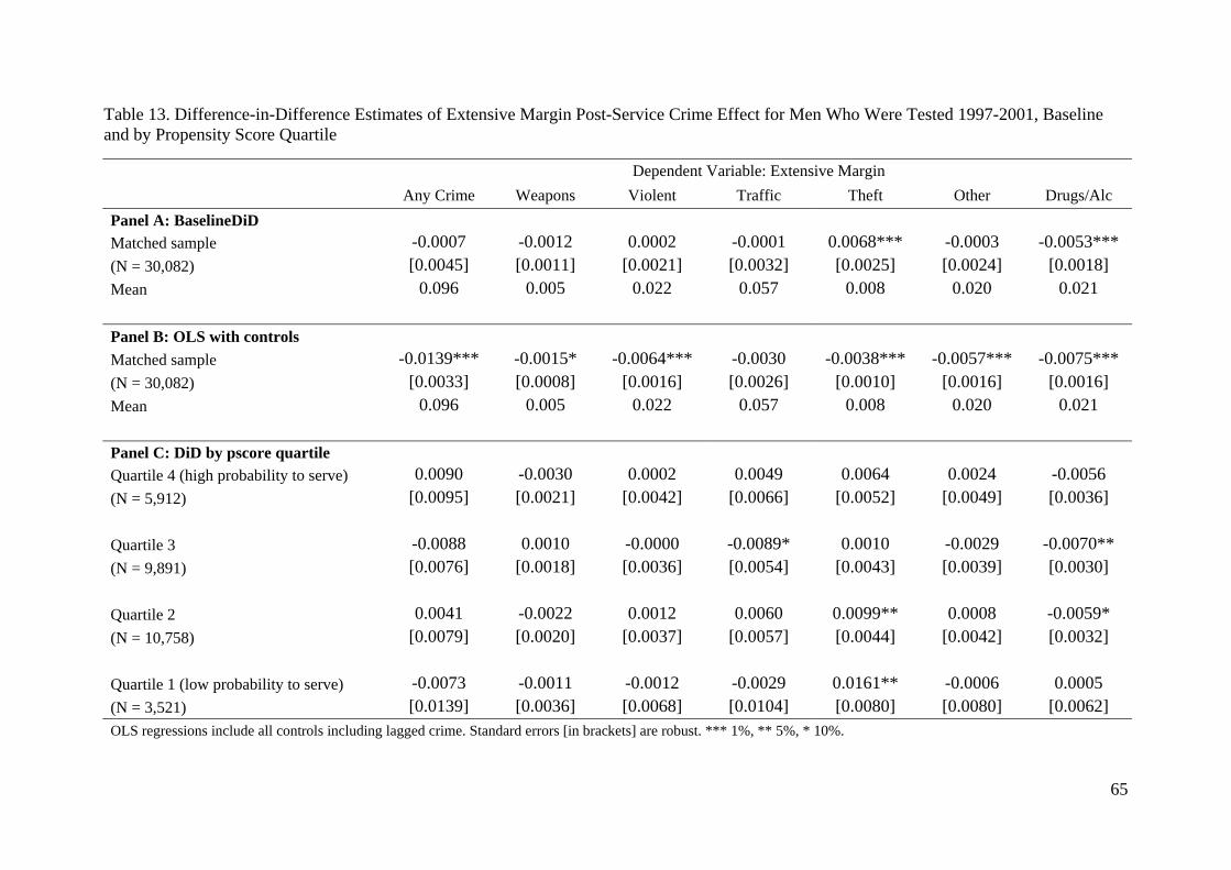
65

Table 13. Difference-in-Difference Estimates of Extensive Margin Post-Service Crime Effect for Men Who Were Tested 1997-2001, Baseline and by Propensity Score Quartile

Dependent Variable: Extensive Margin

Any Crime Weapons Violent Traffic Theft Other Drugs/Alc

Panel A: BaselineDiD

Matched sample -0.0007 -0.0012 0.0002 -0.0001 0.0068*** -0.0003 -0.0053*** (N = 30,082) [0.0045] [0.0011] [0.0021] [0.0032] [0.0025] [0.0024] [0.0018] Mean 0.096 0.005 0.022 0.057 0.008 0.020 0.021

Panel B: OLS with controls Matched sample -0.0139*** -0.0015* -0.0064*** -0.0030 -0.0038*** -0.0057*** -0.0075*** (N = 30,082) [0.0033] [0.0008] [0.0016] [0.0026] [0.0010] [0.0016] [0.0016] Mean 0.096 0.005 0.022 0.057 0.008 0.020 0.021

Panel C: DiD by pscore quartile

Quartile 4 (high probability to serve) 0.0090 -0.0030 0.0002 0.0049 0.0064 0.0024 -0.0056 (N = 5,912) [0.0095] [0.0021] [0.0042] [0.0066] [0.0052] [0.0049] [0.0036] Quartile 3 -0.0088 0.0010 -0.0000 -0.0089* 0.0010 -0.0029 -0.0070** (N = 9,891) [0.0076] [0.0018] [0.0036] [0.0054] [0.0043] [0.0039] [0.0030] Quartile 2 0.0041 -0.0022 0.0012 0.0060 0.0099** 0.0008 -0.0059* (N = 10,758) [0.0079] [0.0020] [0.0037] [0.0057] [0.0044] [0.0042] [0.0032] Quartile 1 (low probability to serve) -0.0073 -0.0011 -0.0012 -0.0029 0.0161** -0.0006 0.0005 (N = 3,521) [0.0139] [0.0036] [0.0068] [0.0104] [0.0080] [0.0080] [0.0062] OLS regressions include all controls including lagged crime. Standard errors [in brackets] are robust. *** 1%, ** 5%, * 10%.

66

Table 14. Potential Peer Effects in Crime.

Dependent variable: Any crime between ages 23-30 Number of crimes between ages 23-30 (1) (2) (3) (4) (5) (6) (7) (8) Unit pre-service crime 0.029 0.0079 0.024 -0.027 0.053** -0.037* 0.007 -0.019 [0.0194] [0.0191] [0.0213] [0.0452] [0.0250] [0.0194] [0.0251] [0.0323] Own pre-service crime = 1 0.115*** 0.089*** 0.115*** 0.115*** 0.454*** 0.2442*** 0.455*** 0.454*** [0.0037] [0.0109] [0.0037] [0.0037] [0.0249] [0.0470] [0.0249] [0.0249] Father education <= 9 years -0.002 -0.042** [0.00061] [0.0205] Private or corporal = 1 -0.007 -0.023** [0.0050] [0.0113] Unit pre-service crime * Own pre-service crime = 1 0.201** 0.748*** [0.0809] [0.1832] Unit pre-service crime * Father education <= 9 years 0.022 0.192** [0.0456] [0.0790] Unit pre-service crime * Private or corporal = 1 0.068 0.083* [0.0502] [0.0430] Mean dependent variable 0.093 0.093 0.093 0.093 0.213 0.213 0.213 0.213 Mean unit crime 0.123 0.123 0.123 0.123 0.262 0.262 0.262 0.262 If pre-service crime = 1 / = 0 0.131/0.122 0.284/0.259 If father education <= 9 years / > 9 years 0.129/0.121 0.280/0.256 If private or corporal = 1 / = 0 0.128/0.067 0.274/0.116 Observations 102,085 102,085 102,085 102,085 102,085 102,085 102,085 102,085 Robust standard errors in brackets; *** p<0.01, ** p<0.05, * p<0.1. This utilizes sample of individuals who tested from 1990-1996 (i.e. the IV sample) who served. All specifications include the full set of test day and pre-test day controls as well as birth month, birth year, municipality and test year by test office fixed effects. Columns (3) and (7) exclude controls for father’s years of schooling, which is one of our pre-test day controls, instead using the dummy for fathers having nine or less years of education. Note that unit pre-service crime is the leave out mean crime rate for each individual’s unit, as defined by test year, rank, and regiment cells.

67

Appendix Table 1. Sample Restrictions for Baseline Instrumental Variable Analysis Sample Restriction Sample Size Non-immigrant males born 1964-1990, and tested 1990-1996 231,707 Excluding if missing county identifier 231,583 Keep only those who are assigned to service 190,520 Drop testees with officiators who see less than 100 cases in their test year

183,065

Drop those missing health group information or assigned to health groups that 'never' serve in that year

173,601

Drop those with unknown end year of service and those 23 or older in year finish service

168,818

This figure provides sample criteria used in creating the baseline sample used in the high service rate officiator instrumental variable analysis.

68

Appendix Table 2. Sensitivity Analysis of Baseline Specification to Standard Error Clustering and Alternative Instrument (1) (2) (3) (4) (5) Panel A: Dependent Variable = Any Crimes from Age 23-30 (Mean = 0.10) military_service 0.08908* 0.08908** 0.08908 0.08908* 0.05707**

[0.04779] [0.04104] [0.05673] [0.04731] [0.02613]

Panel B: Dependent Variable = # Crimes from Age 23-30 (Mean = 0.31) military_service 0.55856** 0.55856** 0.55856** 0.55856** 0.54830***

[0.25192] [0.24409] [0.28332] [0.26652] [0.18881]

Instrument high service

officiator high service

officiator high service

officiator high service

officiator leave out annual

mean

Cluster Unit officiator county 2 way: officiator

and test year officiator x test

year officiator Number of clusters 67 24 67 and 7 203 67 First Stage F-Statistic 32 116 45 39 79 county x test year fixed effects yes yes yes yes yes Test office Fixed Effects no no no no no Pre-test and Test day Controls no no no no no

Columns (1) - (4) present the results of instrumenting for service with a high service rate officiator dummy while column (5) uses the leave out annual mean, i.e. the actual share of testees assigned to an officiator in a given year, excluding the candidate under consideration, who are assigned to service. Standard errors are clustered, and first stage f-statistics calculated accordingly, according to the notes in the table. *** significant 1%, ** significant 5%, * significant 10%. N= 168806

69

Appendix Table 3. Post-Service (23-30) Crime for IV Incapacitation Analysis Sample Dependent Variable:

(1) (2) (3) (4) (5) (6) (7) Any Crime Weapons Violent Traffic Theft Other Drugs/Alc extensive margin: crimes 23-30 Sample: all 18 year old testees 0.06037 0.00473 0.04644** 0.00923 0.00219 0.00984 0.00981

(N = 138799) [0.04448] [0.01096] [0.01898] [0.03285] [0.01597] [0.02344] [0.01773]

Mean Dependent Variable 0.1 0.005 0.023 0.063 0.013 0.024 0.016 intensive margin: crimes 23-30 Sample: all 18 year old testees 0.44435 -0.02081 0.10243* 0.02306 0.11297* 0.13449* 0.09222

(N = 138799) [0.36139] [0.02658] [0.05771] [0.18322] [0.06258] [0.06936] [0.08653]

Mean Dependent Variable 0.3 0.009 0.045 0.12 0.036 0.045 0.046

Robust standard errors, clustered on officiator. *** 1%, ** 5%, * 10*. This table focuses on the sample who took the test at age 18 (and likely served from ages 19-20); i.e. the sample used to isolate incapacitation. But rather than looking at crimes comitted potentially during service, this table looks at post-service crimes (age 23-30) to demonstrate the comparability of the incapacitation sample to the entire sample. Military Service is instrumented for with the high service rate officiator dummy. F-statistic on first stage regressions: 26 for all 18 year old testees. Each regression controls for test year dummies, county dummies and test year x county dummies.

70

Appendix Table 4. Difference-in-Difference Estimates of Intensive Margin Post-Service Crime Effect for Men Who Were Tested 1997-2001, Baseline and by Propensity Score Quartile Dependent Variable: Intensive Margin

Any Crime Weapons Violent Traffic Theft Other Drugs/Alc

Panel A: Baseline DiD Matched sample -0.0789*** -0.0035** -0.0051 -0.0129 0.0198*** -0.0043 -0.0310*** (N = 30,082) (0.0203) (0.0016) (0.0048) (0.0089) (0.0068) (0.0052) (0.0074) Mean 0.262 0.008 0.040 0.104 0.017 0.034 0.059

Panel B: OLS with controls Matched sample -0.1011*** -0.0039*** -0.0177*** -0.0202** -0.0111*** -0.0153*** -0.0328*** (N = 30,082) (0.0201) (0.0014) (0.0043) (0.0085) (0.0037) (0.0040) (0.0073) Mean 0.262 0.008 0.040 0.104 0.017 0.034 0.059

Panel C: DiD by pscore quartile

Quartile 4 (high probability to serve) -0.0830** -0.0039 -0.0007 -0.0156 0.0012 -0.0087 -0.0260** (N = 5,912) (0.0343) (0.0026) (0.0085) (0.0136) (0.0157) (0.0086) (0.0114) Quartile 3 -0.0703** -0.0000 -0.0044 -0.0161 0.0197 -0.0008 -0.0298*** (N = 9,891) (0.0273) (0.0025) (0.0070) (0.0121) (0.0123) (0.0070) (0.0106) Quartile 2 -0.0853** -0.0054* -0.0066 -0.0014 0.0251** -0.0064 -0.0396*** (N = 10,758) (0.0348) (0.0031) (0.0082) (0.0152) (0.0102) (0.0103) (0.0131) Quartile 1 (low probability to serve) -0.0881 -0.0074 -0.0098 -0.0390 0.0400* -0.0001 -0.0226 (N = 3,521) (0.0970) (0.0066) (0.0216) (0.0437) (0.0212) (0.0206) (0.0345) OLS regressions include all controls including lagged crime. Standard errors [in brackets] are robust. *** 1%, ** 5%, * 10%.