the celestial mechanics approach: application to data of

J Geod (2010) 84:661–681DOI 10.1007/s00190-010-0402-6

ORIGINAL ARTICLE

The celestial mechanics approach: application to dataof the GRACE mission

Gerhard Beutler · Adrian Jäggi · Leoš Mervart ·Ulrich Meyer

Received: 12 February 2010 / Accepted: 29 July 2010 / Published online: 21 August 2010© Springer-Verlag 2010

Abstract The celestial mechanics approach (CMA) has itsroots in the Bernese GPS software and was extensively usedfor determining the orbits of high-orbiting satellites. TheCMA was extended to determine the orbits of Low EarthOrbiting satellites (LEOs) equipped with GPS receivers andof constellations of LEOs equipped in addition with inter-satellite links. In recent years the CMA was further devel-oped and used for gravity field determination. The CMA wasdeveloped by the Astronomical Institute of the Universityof Bern (AIUB). The CMA is presented from the theoret-ical perspective in (Beutler et al. 2010). The key elementsof the CMA are illustrated here using data from 50 days ofGPS, K-Band, and accelerometer observations gathered bythe Gravity Recovery And Climate Experiment (GRACE)mission in 2007. We study in particular the impact of (1)analyzing different observables [Global Positioning System(GPS) observations only, inter-satellite measurements only],(2) analyzing a combination of observations of different typeson the level of the normal equation systems (NEQs), (3)using accelerometer data, (4) different orbit parametrizations(short-arc, reduced-dynamic) by imposing different constra-ints on the stochastic orbit parameters, and (5) using either the

G. Beutler (B) · A. Jäggi · U. MeyerAstronomical Institute, University of Bern, Sidlerstrasse 5,3012 Bern, Switzerlande-mail: [email protected]

L. MervartInstitute of Advanced Geodesy, Czech Technical University,K-152, FSvCVVT Thakurova 7, 16629 Prague 6-Dejvice,Czech Republic

inter-satellite ranges or their time derivatives. The so-calledGRACE baseline, i.e., the achievable accuracy of the GRACEgravity field for a particular solution strategy, is establishedfor the CMA.

Keywords Celestial mechanics · Orbit determination ·Global gravity field modeling · CHAMP · GRACE-K-Band ·GRACE accelerometers

1 Introduction

The celestial mechanics approach (CMA) has its roots in theBernese GPS Software (Dach et al. 2007) and it is extensivelyused in this context since 1992 for determining the orbits ofGNSS (Global Navigation Satellite Systems) by the Centerfor Orbit Determination in Europe (CODE) of the Interna-tional GNSS Service (IGS). The CMA was generalized todetermine the orbits of Low Earth Orbiting satellites (LEOs)and constellations of LEOs by Jäggi (2007) using the GPSobservable. In recent years the CMA was extended to grav-ity field determination, including the use of highly accurateinter-satellite measurements.

The theoretical foundations of the CMA may be found inBeutler et al. (2010). Technical aspects like orbit integration,the efficient solution of the variational equations, etc., areoutlined in that reference.

The present article has the focus on the special featuresof the CMA using GPS, K-Band, and, optionally, acceler-ometer data gathered by the GRACE mission in 2007. Itis not the intention of this article to compare the solutionsgenerated by the CMA to those generated by other groups.Such comparisons are, e.g., available in Prange et al. (2010)and Jäggi et al. (2010), where the emphasis is on particular

123

662 G. Beutler et al.

solutions generated with the CMA, which have to be com-pared and/or validated using solutions generated by othergroups. The results presented here are related to the optionsoffered by the CMA and, to some extent, to the methodsof celestial mechanics as such—applied to orbit and forcefield determination. This article is obliged to the Cartesian“discours de la méthode” (Descartes 1637).

Section 2 describes the data set analyzed, the a priorigravity field used and the gravity field to which the solu-tions are compared. The section introduces moreover themethods of comparing and validating solutions. Section 3summarizes the characteristics of all solutions studied sub-sequently.

Section 4 deals with orbit determination of single satellitesusing spaceborne GPS and with orbit determination of closeconstellations using inter-satellite distance measurements inaddition to GPS. The analysis scheme presented in this sec-tion is probably closely related to the one, which would beused by most analysts when tasked with precise orbit deter-mination of a GRACE-like constellation of satellites. Theresults of this section are also used to define the mutual scal-ing of the GPS- and K-Band-specific normal equation sys-tems (NEQs).

Section 5 introduces the standard analysis used so far toderive gravity fields with the CMA. CMA orbits are continu-ous by construction over the entire time span of one arc. Thearc-length for analyzing data from the satellite missions iscurrently 1 day. The orbits are solutions of the deterministicequations of motion. By introducing instantaneous velocitychanges (pulses) in the radial (R), along-track (S), and out-of-plane (W ) directions or, alternatively, piecewise constantaccelerations in these directions, the CMA orbits are givenstochastic properties—for details we refer to Beutler et al.(2010). Section 6 studies the impact of solutions with freeversus constrained pulses or accelerations.

The accelerometer measurements of the GRACE missionand their impact on gravity field estimation are studied inSect. 7. All gravity field solutions discussed up to Sect. 7are based on the K-Band range-rate observable. AlternativeK-Band observables, namely, ranges, range differences, andrange double-differences, are studied in Sect. 8.

The K-Band residuals of range and range-rate solutionsare analyzed in Sect. 9. From the theoretical point of view theK-Band range would be the primary observable—all otherobservables are derivatives of it. The standard range solu-tions presented in Sect. 8, however, cannot cope in qualitywith the best range-rate solutions. In Sect. 10 we show thatrange solutions of a quality comparable to the range-rate solu-tions can be generated with the CMA by making extensiveuse of the pseudo-stochastic parametrization.

The so-called GRACE-baseline (achievable accuracy ofthe gravity field with GRACE) is studied in Sect. 11 as a

function of the CMA options. The major findings are sum-marized in Sect. 12.

2 Observations, reference solutions, comparisons

The GPS-derived kinematic satellite positions of the GRACEsatellites, the K-Band measurements (ranges, range-differ-ences, range-double-differences, range-rates) between themand, optionally, the accelerometer measurements of the mis-sion are used for orbit and gravity field determination in thisarticle. Data from days 50–99 of the year 2007 (DOY 50–99)are analyzed.

The gravity field AIUB-GRACE02Sp (Jäggi et al. 2009),estimated previously at the Astronomical Institute of theUniversity of Bern (AIUB) with the CMA, is used as a pri-ori information (and not modified for the orbit determina-tion runs). The solutions generated in the following sectionsare compared to the solution AIUB-GRACE02S (Jäggi et al.2010). The solution with the suffix “p” is based on the datafrom 2007, the solution without this suffix on data from 2006and 2007. Apart from that the solutions were generated usingthe same pattern. The solution AIUB-GRACE02S

• is a biennial solution (with data from 2006 and 2007);• was generated using the kinematic positions of GRA-

CE-A and -B, the K-Band range-rates without taking themathematical correlations into account, and the acceler-ometer measurements as empirically given (determinis-tic) functions (for a discussion of correlations of K-Bandmeasurements we refer to Beutler et al. (2010));

• was generated with a fixed scaling ratio of σ 2kbd,rr/σ

2ph =

10−10 s−2 between the daily K-Band- and GPS- NEQs;• solved for all spherical harmonic coefficients between

degrees 2 ≤ n ≤ 150 without imposing any constraintsor regularization on them;

• used the gravity field EGM96 (Lemoine et al. 1997) asthe a priori field—and the solution was produced in onestep;

• solved for piecewise constant accelerations in the threedirections R, S and W , set up at 15 min intervals;

• constrained the mean residual accelerations to3 × 10−9 m/s2 in the R-, S-, and W -directions;

• used accelerometer data in the R- and S- directions, butignored them in the W -direction (see Sect. 7);

• constrained the differences between simultaneous accel-erations of the same type between GRACE-A andGRACE-B to 3×10−11m/s2 for the R-, S-, and W - direc-tions.

The quality of the estimated gravity fields is assessed bythe so-called difference degree amplitudes �ai ,

123

The celestial mechanics approach 663

�a2i

.=i∑

k=0

[(Cik,est − Cik,ref)

2 + (Sik,est − Sik,ref)2], (1)

where i is the degree of the spherical harmonics coefficients,k the order; “ref” stands for the reference, “est” for the esti-mated coefficients. In order to study the behavior of specificterms of the expansion the definition (1) is generalized in thefollowing way:

�a2i;l(i),u(i)

.=u(i)∑

k=l(i)

[(Cik,est − Cik,ref

)2

+ (Sik,est − Sik,ref

)2], (2)

where l(i) and u(i) are the lower and upper summation lim-its for each degree. For l(i) = u(i) = 0 the behavior ofthe zonal terms is considered, for l(i) = u(i) = i thatof the sectorial terms. For l(i) = 0 and u(i) = i for-mula (2) reduces to the normal difference degree ampli-tudes, for l(i) = ik and u(i) = ik, ik �= 0 the tesseralterms of a particular order are studied as a function of thedegree.

The square roots of the formal error degree variances,

σ 2i

.=i∑

k=0

[σ 2(Cik,est) + σ 2(Sik,est)

], (3)

or briefly the error degree amplitudes, are used as a roughmeasure of the RMS error of the degree difference ampli-tude �ai (covariances neglected). In analogy to Eqs. (1, 2)degree-specific limits will also be used in Eq. (3).

3 Solutions performed

The solutions generated here are based on the a priori gravityfield AIUB-GRACE02Sp complete up to degree n = 150,but determine only the gravity field up to degree n = 60.Such a set-up might make sense to study monthly variationsin the GRACE gravity field. This aspect is, however, not in thecenter of our interests. We use this option to generate manydifferent solutions in an efficient way (concerning CPU timeand storage requirements).

Table 1 lists all solutions made. The problem type (orbitor gravity field determination), the observable kind(s), theNEQ scaling ratio, the satellite(s), the use of the accelerome-ter data, the type of stochastic parameters, and the constraintsimposed on the mean values and on the differences [definitionsee Beutler et al. 2010, Eq. (33)] of the orbit and stochasticparameters may be reconstructed from the solutions’ names.The actual solutions are in addition time-tagged (year and dayof the year for daily solutions, DOY/2007 for first and lastday included for gravity field determination). When apply-ing the constraints, the value σ0 of the weight unit must be

Table 1 Solution with label PTT(GK)SmmSmSd

Label Solution characteristics

PTT(GK)ASmmSmSd General problem characterization

P Problem type

P.= O: Orbit determination

P.= G: Gravity field determination

TT Observables

GA: GPS-derived positions, GRACE-A

GB: GPS-derived positions, GRACE-B

GC: GPS-derived positions, GRACE-A and -B

RG: GPS-derived positions and K-Band ranges

RD: GPS-derived positions and K-Band range-differences

DD: GPS-derived positions and K-Band range-double-differences

RR: GPS-derived positions and K-Band range-rates

GK Ratio σkbd : σph (K-Band : GPS) for NEQconstituents;

Only for types TT = RG, RD, RR

GK = 16: σkbd: σph = 1 × 10−6 (example)

A Treatment of accelerometer measurements

A.= U: Accelerometer measurements Used

A.= N: Accelerometer measurements Not used

S Type of stochastic parameters

S.= P: Pulses

mm Spacing between stochastic pulses ( min)

mm = 15: Spacing between subsequent sto-chastic epochs 15 min

Sm σabs of stochastic parameter for mean stochas-tic parameters

Sm = 34 : σabs = 3 × 10−4

Sd σrel = σabsS × 10−d for relative stochasticparameters

Sd = 12: σrel = σabs × 10−2

specified. For GPS-only solutions we use σ0 = 2mm for theL1 (and L2) phase measurements, when analyzing K-Bandrange-rates or a combination of GPS and range-rates σ0 =0.2 µm/s. Other combinations of observables are consideredin Sect. 8. The corresponding values for σ0 are specified inEq. (12).

Table 2 contains the list of solutions (without time tags)actually analyzed in each section.

The experiments listed in Table 2 were usually comparedto the biennial solution AIUB-GRACE02. One should keepin mind that this solution does not contain time variationsof the gravity field. Our results thus might be obstructedby this neglect. But as we usually compare two or moresolutions, and are in principle only interested in the mutual

123


Table 2 Solutions performed Label Section Comments

OGXUP15 4 Orbit det. using kinematic positions of GRACE-X, X ∈ {A, B, C},pulses with 15 min spacing, no constraints, accelerometers used.

ORRxxUP15 4 Orbit det. using only K-Band range-rates pulses with 15 min spacing,weak constraints, accelerometers used.

GGCUPmm 5 Gravity field det. using kinematic positions, pulses with spacing of mmmin, mm ∈ {5, 15, 30} min, with accelerometers, no constraints for30 min, and 15 min solutions, weak constraints for 5 min solutions.

GGCUP053810 5 Gravity field det. using only GPS (GRACE-A and GRACE-B), pulseswith 15 min spacing, with accelerometers, weak constraints.

GRRxxUPmm 5 Gravity field det. using only K-Band range-rates pulses with mm minspacing, mm ∈ {5, 15, 30} min, with accelerometers, weak constraints.

GRR14UPmm 5 Gravity field det. using GPS and K-Band range-rates σK B D,rr /σph =1 × 10−4, pulses with spacing of mm min, mm ∈ {5, 15, 30} min, withaccelerometers, weak/no/no constraints.

GRR14UP051610 6 Gravity field det. using K-Band range-rates and GPS, pulses with 5 minspacing, with accelerometers, constraints σvl = 1 × 10−6 m/s for meanvalues and for half differences of pulses.

GRR14UP051612 6 Gravity field det. using only K-Band range-rates, pulses with 5 minspacing, with accelerometers, constraints σvl = 1 × 10−6 m/s for meanvalues and σvl = 1 × 10−8 m/s for half differences of pulses.

GGCNPmm 7 Gravity field det. using only GPS (GRACE-A and GRACE-B), pulses,without accelerometers, pulses with spacing of mm min, mm ∈{5, 15, 30} min, weak/no/no constraints.

GRR14NPmm 7 Gravity field det. using GPS and K-Band range-rates, pulses with spac-ing of mm min, mm ∈ {5, 15, 30} min, with accelerometers, weak/no/noconstraints.

GRR14NP051612 7 Gravity field det. using GPS and K-Band range-rates, pulses with spac-ing of �tp = 5 min, without accelerometers, constraints σvl = 1 ×10−6m/s for mean values and σvl = 1 × 10−8 m/s for half differencesof pulses.

GRD54UP30 8 Gravity field det. using GPS and K-Band range differences,σK B D,rd/σph = 5 × 10−4, pulses with 30 min spacing, accelerometerdata used, no constraints.

GDD84UP30 8 Gravity field det. using GPS and K-Band range-double-differences,σK B D,rdd/σph = 8 × 10−4, pulses with 30 min spacing, accelerom-eter data used, no constraints.

GRG34UP30 8 Gravity field det. using GPS and K-Band ranges without correlations,σK B D,r /σph = 3.46×10−4, pulses with 30 min spacing, accelerometerdata used, no constraints.

GRG33UP30 8 Gravity field det. using GPS and K-Band ranges with correlations,σK B D,r,1a/σph = 2.53 × 10−3, pulses with 30 min spacing, accel-erometer data used, no constraints.

performance of them, this neglect does not affect our mainfindings.

4 Standard processing for orbit determination

Orbits are determined separately for GRACE-A andGRACE-B using only the GPS-derived kinematic positionsas pseudo-observations. Solutions OGAUP15, OGBUP15,OGAUA1539 (see Table 2), are solutions of this kind. Noattempt was made here to improve the GPS-derived posi-tion differences between GRACE-A and GRACE-B, e.g., bysolving for the initial phase ambiguities of the GPS phasedifference observations as recorded by the GRACE-A and-B receivers. Experiments of this type were performed byJäggi (2007).

Orbits for the constellation may be determined usingthe kinematic positions and the K-Band observations. In theexperiments performed in this section the accelerometermeasurements were introduced as empirically givenand the following accelerometer-specific parameters weredetermined:

• one offset parameter per day in the directions R and W ,• a polynomial of degree q = 3 in the S-direction to absorb

slow time variations of the bias parameter,• once-per-revolution terms in R, S, and W .

It is in principle possible to solve for a scale parameter. Thisoption was not used subsequently (mainly due to strong cor-relations with the once-per-rev parameters).

It is not possible to determine the orbits of the two sat-ellites by analyzing only K-Band data and to solve for all

123


0.001

0.0012

0.0014

0.0016

0.0018

0.002

0.0022

0.0024

50 60 70 80 90 100

day of year 2007

GPS,GRACE-A

GPS,GRACE-B

GPS,GRACE-C

K-Band-RR*10000

1e-008

1.5e-008

2e-008

2.5e-008

3e-008

3.5e-008

50 60 70 80 90 100

day of year 2007

ratio

Fig. 1 Left: RMS error of orbit determination using GRACE-A kine-matic positions (m), GRACE-B kinematic positions (m), GRACE-Aand GRACE-B kinematic positions (m), and K-Band range-rates (m/s,

multiplied by 104). Solutions OGAUP15yyddd, OGBUP15yyddd, OG-CUP15yyddd, ORRUP15yyddd; right: Derived ratio σ 2

kbd/σ 2gps using

GRACE-C

orbit parameters pertaining to the two satellites—the corre-sponding NEQ-matrix would become singular. A non-sin-gular differential orbit determination problem using only theK-Band observations is defined by solving only for the dif-ferences p2 [Beutler et al. 2010, Eqs. (33)] of the orbit andstochastic parameters pertaining to the satellites, GRACE-A and GRACE-B, and by slightly constraining the differ-ences of the corresponding orbit parameters to the a prioriGPS-derived orbit parameters. This scheme makes sense,because the K-Band observations are only very weaklydependent on the mean values p1 of the orbit parametersand because they are almost uniquely sensitive to theS-direction (see Eqs. (33)). The K-Band-only solution bearsthe label ORRxxUA153912, “xx” standing for a zero weighton the GPS NEQs. The square of the ratio of the GPS-and K-band-only RMS values a posteriori may subsequentlyserve as the weight factor when combining GPS- and K-BandNEQs.

Figure 1 (left) shows the RMS errors a posteriori [GPSL1 phase observable, see Beutler et al. 2010, Sect. 3.2] ofthe daily orbit determination steps OGAUP15, OGBUP15,OGCUP15, and ORRxxUP15 (the latter multiplied by a fac-tor of 104) as a function of the day of the year. The RMSerrors of the GPS-only solutions for GRACE-A and GRACE-B reveal essentially the same pattern as a function of timeas the two satellites have almost identical properties, are innearly the same orbital plane and observe simultaneouslythe same GPS satellites. Figure 1 (left) shows in additionthe RMS of the GPS-only solutions using the GRACE-Aand GRACE-B GPS-data together (solution OGCUP15, labelGRACE-C). The latter RMS errors were used as σph to derivethe ratio σ 2

kbd/σ 2ph for each day.

Figure 1 (right) shows the day-specific ratios σ 2kbd/σ 2

ph forthe GPS- and K-Band-specific NEQ contributions derived

-1.5

-1

-0.5

0

0.5

1

1.5

0 200 400 600 800 1000 1200 1400

um/s

Minutes of day 62, 2007

15 min 5 min

Fig. 2 Residuals of K-Band range-rate observations (µm/s) using apulse spacing of 15 and 5 min, respectively, DOY 62

from the RMS errors of solutions OGCUP15yyddd and OR-RxxUPyyddd in Fig. 1 (left). These values are used whenanalyzing GPS- and K-Band range-rate data together andparametrizing the orbits with pulses (spacing of 15 min, noconstraints). Figure 2 shows that the pattern of the range-rateresiduals and the corresponding RMS error depends some-what on the spacing of the pulses. The systematic effects stillpresent in the solution with a spacing of 15 min obviously canbe absorbed to some extent by reducing the spacing from 15to 5 min.

As the orbit and gravity field determinations are not verysensitive to small variations of the weight ratio within, letus say, a factor of 3, a general ratio of σ 2

ph/σ 2ph

.= 10−8s−2

will be used subsequently. Note that this ratio does not givethe best consistency of our gravity fields with those of otherGRACE analysis teams. Values of the order of σ 2

kbd/σ 2ph ≈

10−10s−2, in essence de-weighting the GPS-contributions,make our results more consistent to those of other groups.

123


This issue is, however, not of interest for the subsequentexperiments.

Figures 1 and 2 document the simplest analysis scheme inorbit (and gravity field) determination, the short-arc scheme:The daily arc is subdivided into contiguous short arcs of�tp min, where �tp = 15 min in the example. A simi-lar experiment was performed by replacing the pulses bypiecewise constant accelerations with the same spacing as thepulses. Slightly smaller ratios of about σ 2

kbd/σ 2ph ≈

(0.5–1.5) × 10−8 s−2 could be achieved.

5 Standard processing for gravity field determination

Gravity field analysis may either be based on the GPS aloneor on a combination of the GPS and the K-Band observables.Although this is not really correct, one may also use only theK-Band NEQs to derive a gravity field in analogy to the dif-ferential orbit determination strategy introduced in Sect. 4.Solutions of this kind will be generated here in order to vali-date the K-Band-only and the GPS-only contributions of theestimated gravity fields. As in Sect. 4 the accelerometer mea-surements are used as empirically given deterministic values.The same accelerometer-specific parameters are determinedas in Sect. 4.

In this section the CMA is used to determine the sphericalharmonics coefficients between the degrees 2 ≤ i ≤ 60. Theterms of degrees 61 ≤ i ≤ 150 are taken over and kept fixedfrom the solution AIUB-GRACE02Sp. The coefficients ofdegree n > 150 are set to zero. No constraints or regulariza-tions are put on the estimated gravity field parameters. Theobservations of DOY 50–99/2007 are used in this section—asin Sect. 4.

Gravity fields determined only by the kinematic positionsare documented in Fig. 3. All solutions are based on pulsesin R, S, and W with a spacing of 5, 15 and 30 min, respec-tively. The solutions are compared to the biennial solutionAIUB-GRACE02S using Eq. (1). For reference purpose thesolution EIGEN-05S (Förste et al. 2008) is included, as well.The pulses are unconstrained for the solutions based on the 15and 30 min intervals. It was necessary to put weak constraintsof 10−4 m/s on the 5 min solution to avoid true singularitiesdue to data outages, because a linear dependency is intro-duced if two pulses are set up at times ta and tb and if thereare no kinematic positions in the interval [ta, tb]. The con-straints imposed on the 5 min pulses are weak enough not toinfluence the resulting gravity field significantly. The solidlines in Fig. 3 show the difference degree amplitudes of thethree short-arc solutions w.r.t. the biennial solution AIUB-GRACE02S. The quality of the three solutions is almost thesame between the degrees 15 < i < 50. The lower degreesagree better with AIUB-GRACE02S for a wider spacing of

0 10 20 30 40 50 6010

−12

10−10

10−8

10−6

degree n

AIUB−GRACE02SGGCUP055099GGCUP055099GGCUP155099GGCUP155099GGCUP305099GGCUP305099EIGEN−05S

Fig. 3 Difference degree amplitudes w.r.t. AIUB-GRACE02S (solid)and error degree amplitudes (dash-dot) of GPS-only gravity fields basedon short-arcs of 5, 15, and 30 min length; EIGEN-05S difference degreeamplitudes w.r.t. AIUB-GRACE02S included for reference

the pulses, for the degrees n > 50 the opposite is true. Thedash-dot lines in Fig. 3, showing the error degree amplitudesaccording to Eq. (3), explain the quality patterns of the threesolutions for the low degree terms: setting up more and moreunconstrained or only weakly constrained pulses does notallow it to the parameter estimation process to distinguishbetween the long-wave gravity field terms and a long wave-length signal, which may be absorbed by the pulses. Thishas to be expected, because signals with periods P > �tp

may very well be absorbed by the pulses. One might ask thequestion whether the offset between the three curves is signif-icant. Both answers, positive and negative, may be given: Thedash-dot curves in Fig. 3 are computed from the RMS errors aposteriori, i.e., they reflect the product of the estimated meanerror a posteriori of the observations and the square roots ofthe diagonal elements of the corresponding cofactor matrix,the inverse NEQ matrix. In a covariance study based on thewhite noise assumption one would replace the three RMSerrors a posteriori by one and the same RMS error a priori.In this case the three error degree amplitudes would practi-cally coincide in the interval of degrees 15 < n < 50. In thepresence of biases in the kinematic positions more and moreof the low-frequency systematics may be absorbed by thepulses, implying that the mean errors a posteriori decreasewith decreasing pulse separation �tp (1.89, 1.36, 0.89mmfor �tp = 30, 15, 5 min in our case) —and the three errordegree amplitude curves should be different. The “abnormal”behavior of the error degree variances for the degrees 59 and60 is caused by the cut-off degree n = 60 in the estimationprocess.

Figure 4 shows that GPS determines the sectorial terms ofthe gravity field much better than the zonal terms, becausethe sectorial terms generate long-wave perturbations along apolar orbit. Figure 4 shows that the RMS errors of the grav-ity field coefficients drop by 1–3 order of magnitude fromthe zonal to the sectorial terms. This fact indicates that the

123


−80 −60 −40 −20 0 20 40 60 80

0

10

20

30

40

50

60

70

S <−− order −−> C

degr

ee

−16

−15

−14

−13

−12

−11

−10

−9

−8

−7

Fig. 4 Formal RMS errors of spherical harmonics coefficients (loga-rithmic scale) of solution GGCUP15

difference degree amplitudes and the corresponding errordegree amplitudes in Fig. 3 usually are dominated by theerror amplitudes in the (close to) zonal terms.

Instead of introducing and solving for the two satellite-specific orbit and stochastic parameter sets o1 and o1 theirmean values p1 = (o1 + o2)/2 and half differencesp2 = (o1−o2)/2 are used as parameters in the CMA [Beutleret al. 2010, Eq. (33)]. This parameter transformation has sev-eral advantages. Here we make use of the fact that p1 is almostuniquely determined by the GPS observations, whereas p2

is mainly determined by the K-Band observations. There-fore, the mean values p1 were left out (i.e., kept fixed onthe a priori values determined by GPS) from the full set oforbit and stochastic parameters for the K-Band-only solu-tion. Weak constraints were put on the parameters p2, i.e.,on the pulse differences and on the differences of the orbitelements. The following constraints were applied on halfthe differences of the initial osculating elements and of thepulses: σa = 1m, σe = 1 × 10−3, σi = σ� = σω =σu = 10 arcsec, σR = σS = σW = 10−3 m/s. The symbolsa, e, i,�, ω, u stand for the semi-major axis, the numeri-cal eccentricity, the inclination of the orbital plane w.r.t. theequatorial plane, the right ascension of the ascending node,the angular distance of the perigee from the ascending node,and for the argument of latitude, respectively; the symbolsR, S, and W stand for velocity changes (pulses) in the radial,along-track, and out of plane directions. All elements referto the initial epoch. For more details please consult Beutleret al. (2010).

The solid lines in Fig. 5 show the degree difference ampli-tudes of the solutions with 5, 15 and 30 min pulse spac-ing w.r.t. the solution AIUB-GRACE02S, the dash-dot linesshow the corresponding error degree amplitudes. The threesolutions obviously are highly consistent with AIUB-GRACE02S. The consistency increases with the pulse

0 10 20 30 40 50 6010

−12

10−11

10−10

10−9

10−8

degree n

GRRxxUP055099 (diff)GRRxxUP055099 (error)GRRxxUP155099 (diff)GRRxxUP155099 (error)GRRxxUP305099 (diff)GRRUPxx305099 (error)

Fig. 5 Difference degree amplitudes w.r.t. AIUB-GRACE02S (solid)and error degree amplitudes (dash-dot) of range-rate-only gravity fieldsbased on short-arcs of 5, 15, and 30 min length

0 10 20 30 40 50 60

10−12

10−10

10−8

10−6

degree n

GPS, zonal (diff)GPS, zonal (err)KBD, zonal (diff)KBD, zonal (err)GPS, sect (diff)GPS, sect (err)KBD, sect (diff)KBD, sect (err)

Fig. 6 Difference degree amplitudes w.r.t. AIUB-GRACE02S (solid)and error degree amplitudes (dash-dot) of GPS-only (zonal: red, secto-rial: green) and K-Band (range-rate)-only (blue zonal, black sectorial)coefficients based on short-arcs of 15 min length

spacing. The error degree amplitudes are in turn roughly con-sistent with the degree difference amplitudes.

A comparison of Figs. 3 and 5 shows that K-Band hasa much higher potential to contribute to a combined grav-ity field and that the combined gravity field in general isdominated by the K-Band contribution. The contribution is,however, substantially different for different types of har-monic coefficients. Figure 6 illustrates this fact for the 15 minshort-arc solutions: The solid lines of Fig. 6 (red: GPS, blue:K-Band, range-rate) show the degree differences of the zonalterms w.r.t. AIUB-GRACE02S, the dash-dot-lines of thesame color the corresponding error degree amplitudes. Thegreen and black lines in Fig. 6 give the same information forthe sectorial terms, where green corresponds to GPS, blackto K-Band. GPS obviously cannot contribute much to thezonal terms above degree n ≈ 5. It has, however, the poten-tial to contribute up to degree n ≈ 60 (and beyond) to thedetermination of the sectorial terms.

Figure 6 also tells that it is difficult to assess the mutualbenefits of the GPS- and K-Band technique for gravity field

123


determination. The sole use of the difference degree ampli-tudes (1) is not sufficient for a refined analysis.

The next series of solutions combine GPS and K-BandNEQs using the weight ratio of σ 2

ph/σ 2kbd = 108 s2. They

may be considered as the normal or standard GRACE solu-tions. The results are expected to improve w.r.t. those obtainedusing only GPS or K-Band. Figure 7 shows that this is thecase, but not by a large margin (when compared to theK-Band-only contribution). For reference, the correspond-ing solutions based only on K-Band are included (dash-dotlines, same color).

The pattern is rather similar for both types of solutions.The combined solution is slightly superior, in particular forthe low degree terms.

The differences between the K-Band-only and the com-bined solution are shown in Fig. 8 for a 15 min spacing of thepulses. The differences show maximum (absolute) values for

0 10 20 30 40 50 6010

−11

10−10

10−9

10−8

degree n

GRR14UP05GRRxxUP05GRR14UP15GRRxxUP15GRR14UP30GRRxxUP30

Fig. 7 Difference degree amplitudes w.r.t. AIUB-GRACE02S of thecombined GPS- and K-Band (range-rate)-solution (weight ratio =1 × 108); Corresponding K-Band-only solutions included for reference(dash-dot)

−80 −60 −40 −20 0 20 40 60 80

0

10

20

30

40

50

60

70

S <−− order m −−> C

degr

ee n

−16

−15

−14

−13

−12

−11

−10

−9

−8

−7

Fig. 8 Difference between spherical harmonic coefficients ofcombined and K-Band-only solutions (short-arcs of 15 min) (weightratio = 1 × 108)

the (close to) sectorial terms, whereas the differences are onthe RMS level or below for the (close to) zonal terms—exceptfor the terms of very low degree.

Figure 8 shows that GPS has a significant impact on thegravity field determined from the data of the GRACE mis-sion, provided the ratio σ 2

ph/σ 2kbd is defined according to

Sect. 4. For σ 2ph/σ 2

kbd → ∞ the combined gravity field willasymptotically approach the K-Band-only case.

6 Constraining pulses or accelerations in the CMA

Figure 7 showed that the consistency of the 50-day solutionwith solution AIUB-GRACE02S increases with increasingspacing �tp of the pulses, which points to an over-param-etrization when reducing the pulse spacing to values below10 min. As mentioned it was necessary to weakly constrainthe pulses for the 5 min solution in order to avoid true sin-gularities. Whereas constraining was only applied to avoidsingularities in Sect. 5, this option is used here to constrainthe pulses as tightly as allowed by the “physical facts”.

Figure 9 shows the difference degree amplitudes of twoconstrained solutions based on the 5 min pulse solution. Insolution GRR14UP051610 (red curves) all pulses are con-strained to σvl (�t) = 10−6 m/s (RMS error a priori ofthe range-rate observations σ0 = 2 × 10−7 m/s), in solu-tion GRR14UP051612 (blue curves) the mean values of thepulses [see Beutler et al. 2010, Eq. (33)], are constrained tothe same value of σvl (�t), and half of the differences ofthe pulses are more tightly constrained to 10−8 m/s. Notethat velocity changes of 10−6 m/s with a spacing of 300sare roughly equivalent to piecewise constant accelerationsof 10−6/300 ≈ 3.3 × 10−9 m/s2 with the same spacing [seeBeutler et al. 2010, Eq. (17), a value which is clearly abovethe value recommended by Beutler et al. 2010, Eq. (19)]. The

0 10 20 30 40 50 6010

−11

10−10

10−9

degree n

GRR14UP051610GRR14UP051612GRR14UP05GRR14UP15

Fig. 9 Difference degree amplitudes of combined and constrainedshort-arc solutions (short-arcs of 5 min) w.r.t. AIUB-GRACE02S. 5 and15 min unconstrained solutions included for reference (dash-dot curves)

123


large value allows it to absorb possible systematic effects inthe kinematic positions emerging from GPS. The constraintsapplied to the pulse differences are two orders of magni-tude smaller than the constraints applied to the mean valuesof pulses for solution GRR14UP051612, assuming that theerrors to be absorbed by the pulses are highly correlated forGRACE-A and GRACE-B.

For reference the unconstrained (weakly constrained)solutions for the 5 and the 15 min short-arcs are included,as well (green and black curves). Constraining a parameterto zero with infinite weight is equivalent to leaving it out fromthe solution. This explains why the solutions GRR14UP-051610 and GRR14UP051612 are closer in quality to theGRR14UP15 solution (i.e., to the unconstrained 15 min solu-tion). Observe that the consistency with AIUB-GRACE02Sis best for solution GRR14UP051612.

In analogy to Sect. 4 we should generate and discuss thesolutions based on piecewise constant, constrained acceler-ations (as opposed to pulses). As the results are very close tothose based on pulses—provided the constraints are adaptedaccording to (Beutler et al., 2010, Eqs. (17))—this discussionis skipped.

7 Using accelerometer data in the CMA

Figure 10 shows the accelerometer values for DOY 90/2007(mean offsets removed, left: full day, right: 3-h detail view)in m/s2 from top to bottom in the R-, S-, and W -directions forGRACE-A (red), GRACE-B (blue), and for the differencesGRACE-A minus GRACE-B (green). The original measure-ments were transformed from the instrument frame to refer tothe R-, S- and W -directions. The GRACE-B data were more-over shifted by �t = +28 s before taking the differences (�tvaries slowly from day to day). This time shift of the GRACE-B data makes the differences GRACE-A minus GRACE-Brefer (roughly) to the same point in space. Assuming thatthe atmosphere and the insolation did not change much dur-ing �t = 28 s and that the spacecrafts were not acceler-ated artificially during this time interval (e.g., by thrusterfiring), the accelerometers of the two satellites should mea-sure almost the same signal and the difference of the seriesshould be at least an order of magnitude smaller than theindividual signals measured by the GRACE-A and -B accel-erometers.

Figure 10 shows that this expectation is best met for S,not so well for R, and not at all for W (all figures are drawnusing the same scale). The difference signal in S is gen-erally well below the 10−9 m/s2 level (after removal of aconstant offset) and the small spikes usually may be attrib-uted to one of the two satellites. In R, the signal commonto both spacecrafts is clearly visible, but frequent spikes onthe level of about 1 − 2 × 10−8 m/s2 (attributable to one of

the two satellites and thus not reduced by forming the dif-ferences) do occur. In the W -direction the “true” differencesignal is heavily affected by pulses frequently reaching val-ues of > 5 × 10−8 m/s2. The characteristics of the spikesis visible particularly well in Fig. 10 (right). By consult-ing the thruster information file (THR1B*-files), describedin Bettadpur (2007), one can associate virtually all of thesespikes in R, S, and W by (series of) thruster firings leavingtheir traces in the accelerometer data files. The crucial ques-tion is of course, whether these accelerations are real or not.Based on studies of many figures of type Fig. 10 the accel-erometer measurements in the W -direction were excluded,because

• the pattern observed for DOY 90/2007 is typical for allother days of our data set;

• it cannot be excluded that the significantly larger sizesof the spikes in W are due to the reduced measurementaccuracy in this direction (Touboul et al. 1999);

• the W -measurements only have a small impact on theK-Band measurements.

Tests made using and not using the W -accelerations did notreveal significant quality differences.

The differences of the along-track accelerations ofGRACE-A and GRACE-B govern the time development (dueto the non-gravitational forces) of the distance between thesatellites. The differential along-track signal in Fig. 10 (mid-dle row, green) shows the differential signal (essentially) atthe same location. For describing the inter-satellite distancethe plain difference without time shift has to be used. Thecorresponding figure was not included in the interest of short-ening the article.

Our solutions use accelerometer data in a naive sense, byjust interpreting the data in the accelerometer files as valuesof a given empirical function in the numerical integrationprocess. Parameters which may be considered as accelerom-eter-specific in the CMA are: offsets and once-per-revolutionparameters for the R-direction, a polynomial of degree q = 3and once-per-revolution parameters for the S-direction. Thepulses in R and S may be viewed as accelerometer-specific, aswell. Constant, once-per-revolution parameters, and pulsesare also set up for the W -direction. As the accelerometermeasurements in the W -direction are not used, the mentionedparameters define the empirical accelerations in the W -direc-tion. In solutions not making use of accelerometer data thesame parameters in the R- and S-directions are set up as inthe solutions using accelerometer data, but the interpretationis different: they are now the parameters of the empiricalacceleration model in R and S.

For gravity field estimation without and with accelerome-ters the pattern set in Sect. 5 is followed: first, the GPS-onlysolutions without using accelerometer data are generated and

123


-8e-008

-6e-008

-4e-008

-2e-008

0

2e-008

4e-008

6e-008

8e-008

0 200 400 600 800 1000 1200 1400 1600

m/s

**2


-8e-008

-6e-008

-4e-008

-2e-008

0

2e-008

4e-008

6e-008

8e-008

240 260 280 300 320 340 360 380 400 420

m/s

**2


-8e-008

-6e-008

-4e-008

-2e-008

0

2e-008

4e-008

6e-008

8e-008

0 200 400 600 800 1000 1200 1400 1600

m/s

**2


-8e-008

-6e-008

-4e-008

-2e-008

0

2e-008

4e-008

6e-008

8e-008

240 260 280 300 320 340 360 380 400 420

m/s

**2


-8e-008

-6e-008

-4e-008

-2e-008

0

2e-008

4e-008

6e-008

8e-008

0 200 400 600 800 1000 1200 1400 1600

m/s

**2


-8e-008

-6e-008

-4e-008

-2e-008

0

2e-008

4e-008

6e-008

8e-008

240 260 280 300 320 340 360 380 400 420

m/s

**2


GRACE-A, R GRACE-B, R GRACE-(A-B), R GRACE-A, R GRACE-B, R GRACE-(A-B), R

GRACE-A, S GRACE-B, S GRACE-(A-B), S GRACE-A, S GRACE-B, S GRACE-(A-B), S

GRACE-A, W GRACE-B, W GRACE-(A-B), W GRACE-A, W GRACE-B, W GRACE-(A-B), W

Fig. 10 Accelerometer measurements in R-, S-, and W -directions for GRACE-A, GRACE-B and the difference GRACE-A -B, time shifted torefer the measurements to “the same” point in space. Left: full DOY 90/2007, right: 4h–7h , same day

compared to the corresponding solutions making use of theaccelerometer data. Then, the same analysis is performedwith the combined GPS- and K-Band solutions. Apart fromnot using the accelerometer data the background models andthe parametrization for the new solutions are identical withthose documented in Sect. 5. We thus expect to isolate thenet impact of the accelerometer data.

Let us start with the GPS-only results: there is no visibleeffect in the difference degree amplitudes, when compar-ing the solutions with and without accelerometer data withan analogue to Fig. 3. Small differences do, however, exist.Figure 11 visualizes these differences (absolute values, loga-rithmic scale) for the 15 min solutions using a color code. Weconclude that the accelerometer data have very little impact

123


−80 −60 −40 −20 0 20 40 60 80

0

10

20

30

40

50

60

70

S <−− order m −−> C

degr

ee n

−16

−15

−14

−13

−12

−11

−10

−9

−8

−7

Fig. 11 Effect of the accelerometer data on spherical harmonics coef-ficients for the 15 min GPS-only solutions (absolute values, logarithmicscale)

on the quality of the gravity field using only the GPS mea-surements. This result confirms the findings of Ditmar et al.(2007) and Prange et al. (2009).

Figure 12 (left), showing the difference degree ampli-tudes w.r.t. solution AIUB-GRACE02S for the three short-arcsolutions with a spacing of pulses of �t = 5, 15, 30 minneglecting the accelerometer data (solid lines) and the cor-responding solutions making use of the accelerometer data(dash-dot lines), underlines that the accelerometer measure-ments have a significant impact on gravity field determinationwhen using in addition K-Band range-rates, but that solutionsof good quality may also be generated without using thesemeasurements. This result confirms the finding of Jäggi et al.(2010). The quality gain is more pronounced for the higherdegrees than for the lower degrees, because the accelerome-ter-specific parameters successfully remove the low-, but notthe high-frequency systematics. The impact of the acceler-

ometer data becomes more and more prominent with increas-ing spacing �tp of the pulses. For the 30 min-arcs the levelof the degree difference amplitudes w.r.t. AIUB-GRACE02Sis reduced by about 0.15–0.30 in the logarithmic scale, cor-responding to a factor of about 1.4–2.0 in the numeric scale.Figure 12 (right) visualizes the differences of the individualterms estimated with and without the use of the accelerom-eter data. The differences are very small for the low orderterms, they are rather pronounced for the (close to) sectorialterms and the low-degree terms.

8 Analyzing K-Band ranges, range-rates,and range-differences

All solutions involving K-Band were till now based on therange-rate observable without modeling the mathematicalcorrelations between the observations. Alternative solutionsare studied in this section and they are put in relation tothe range-rate solution. Table 3 lists the processing optionsoffered by the CMA. Let us point out that all experimentsperformed here are based on the assumption of white noisefor the original Level-1A range data. Some results involv-ing difference degree amplitudes might be slightly different(worse) when dropping this assumption. The results involv-ing error degree amplitudes are not affected.

Range (options R and RC), range-differences (optionsRD and DD), or range-rate (options R R and R RC) may beused as the basic K-Band observables. Options R, RD, DD,and R R disregard the mathematical correlations introducedby the filtering process to generate Level 1b from Level 1adata [Beutler et al. 2010, Sect. 3.3], options R RC and RCtake them into account. The generic formulas for filtering arerepresented by (Beutler et al., 2010, Eqs. (6)). The resultingweight matrices for range and range-rate Level 1b data aregiven by (Beutler et al., 2010, Eqs. (8) and (9)), respectively.

0 10 20 30 40 50 6010

−11

10−10

10−9

10−8

degree n

GRR14NP05GRR14UP05GRR14NP15GRR14UP15GRR14NP30GRR14UP30

−80 −60 −40 −20 0 20 40 60 80

0

10

20

30

40

50

60

70

S <−− Order m −−> C

degr

ee n

−16

−15

−14

−13

−12

−11

−10

−9

−8

−7

Fig. 12 Combined GPS- and K-Band solutions (weight ratio 1 ×108 s2). Left: Difference degree amplitudes w.r.t. AIUB-GRACE02S(solid lines solutions without accelerometers, dash-dot lines solutions

with accelerometers); right: difference of estimated spherical harmonicscoefficients with and without accelerometer data for the 15 min solution

123


Table 3 CMA processing options for K-Band Analysis

Option Correlations K-band observable

RR No Range-rates

R No Ranges

RD No Range differences

DD No Range-double-differences

RRC Yes Range-rates

RC Yes Ranges

The explicit GRACE filter formulas are given in Thomas(1999).

Formulas (8, 9) in Beutler et al. (2010) suggest that a cor-rect processing of a batch of Level 1b K-Band data (in ourcase a batch corresponds to one day) implies a fully populatedweight matrix P for range and P′ for range-rate, respectively,where the dimension of the weight matrices equals the num-ber of observations. This dimension is d = 86,400/5 =17,280 when analyzing a full day of 5 s data. It is in prin-ciple trivial to implement a procedure to handle correlationscorrectly. Such procedures will, however, become rather inef-ficient when data spans of the order of one day or more aredealt with. To the best of our knowledge, nobody made theattempt to implement correct correlations over intervals ofthis length. We do not have the intention to do that either—also based on the results of this section.

It is, however, easily possible to subdivide the entire timeinterval into shorter subintervals of, let us say, 30 min to2 h, and to use the correct correlation matrices P or P′ withinthese subintervals. This subdivision may, but need not, besynchronized with the stochastic epochs tp. This procedurehas to be understood in the CMA under options RC and R RCfor ranges and range-rates, respectively, where the length ofthe subintervals is set by the user. In order to get a first idea ofthe relevance of correlation modeling the matrices P and P′are visualized for a time interval of 30 min and a data spacingof �t = 5 s.

Figure 13 (left) shows that the weight matrix P for rangeis “almost diagonal”. It is even closely related to P ≈ s × U,where s is a positive scaling factor and U is the unit matrix,where the dimension equals the number of K-Band observa-tions in the subinterval. Using either matrix P or its approx-imation (scaled unit matrix) therefore cannot have too muchof an impact on the results. Options R and RC therefore areexpected to give similar results. Evidence for this statementwill be provided later in this section.

Figure 13 (right) shows that the weight matrix P′ forrange-rate is far from diagonal. Therefore, one concludes atfirst sight that correlations must be taken into account whenanalyzing this observable. One may ask the question, how-ever, whether option R RC is needed at all, when optionsR and RC are available: Apart from first and higher orderterms in �t range-rate equals range-difference between sub-sequent ranges divided by the time difference �t separatingthe ranges

ρ̇i = ρi+1 − ρi

�t+ O(�t), (4)

where �t = 5 s for the GRACE Level 1b data. To the sameorder in �t the second time derivative of range may beapproximated as

ρ̈i = ρi+2 − 2ρi+1 + ρi

�t2 + O(�t). (5)

Equation (5) simply says that analyzing range-double-dif-ferences and range-accelerations (both without taking cor-relations into account) must give almost identical results—assuming that the factor �t2 is taken into account in theweight matrix when combining the GPS- and K-Band-spe-cific NEQs. With option DD it is thus possible to obtain(almost) identical results as those, which would emerge in ananalysis of range-accelerations. The CMA is thus “in princi-ple” capable of generating orbits and gravity fields based onranges, range-rates and range-accelerations using the optionsR, RD, DD. Gravity fields based on the R, RD, and DD

Fig. 13 Weight matrices for atime interval of 30 min with�t = 5 s data spacing (left:K-Band ranges, right: K-Bandrange-rates)

50 100 150 200 250 300 350

50

100

150

200

250

300

350 0

5

10

15

20

25

30

35

40

45

50

50 100 150 200 250 300 350

50

100

150

200

250

300

3501

2

3

4

5

6

7

8

9

10

11x 10

4

123


options will be provided at the appropriate place in this sec-tion. Equation (4) has the following messages:

• The processing options R R and RD are closely related.One obtains, as a matter of fact, almost identical gravityfields (evidence provided below) when using weight fac-tors for the GPS/K-Band combination of NEQs accordingto Eq. (4) when analyzing range-rate or range-differences(both without modeling correlations), respectively.

• The simultaneous use of ranges and range differencesadds no independent information to an analysis based onranges, because the latter observables are linear combina-tions of the former—if the weights of the range-differenceobservations are calculated by applying the law of errorpropagation to the linear combination of ranges on theright-hand side of Eq. (4).

• The situation is different, if the weights are set in a dif-ferent way, e.g., by assigning a much higher weight torange-differences as compared to ranges (than that emerg-ing from Eq. (4)). The CMA allows it to combine range,range-rate solutions, range-accelerations on the NEQ-level with user-defined weights. This option was, how-ever, not studied in this work.

• Equation (4) helps to understand Fig. 13 (right): assum-ing that the Level 1b ranges are independent (not too badan assumption by virtue of Fig. 13 (left)) with varianceσ 2 = 1, the relation between the range differences andthe ranges reads as

�ρ =

⎛

⎜⎜⎜⎜⎜⎜⎝

−1 1 0 . . . 0 00 −1 1 . . . 0 0. . . . . . . . . . . . . . . . . .

. . . . . . . . . . . . . . . . . .

0 0 . . . −1 1 00 0 . . . 0 −1 1

⎞

⎟⎟⎟⎟⎟⎟⎠ρ

.= D ρ. (6)

Under the assumptions mentioned the covariance matrixof the range-differences is cov (�ρ) = DDT , a blockdiagonal symmetric matrix with only the diagonal and theadjacent elements to the diagonal different from zero. Itsinverse (DDT )−1, however, has almost exactly the shapeof Fig. 13 (right)! The shape of matrix P′ is thus mainlydetermined by forming the time differences of the Level1b ranges and does not have much to do with the filter-ing process to generate the Level 1b range-rates from theLevel 1a ranges.

Based on these facts options R and R RC are expected toprovide almost identical results:

1. Biased ranges without correlations (option R) and range-differences with weight matrix (DDT )−1 (not available

as a separate option in the CMA) will inevitably lead toidentical results.

2. Because of Eq. (4) the analysis based on range-rate usingthe correlation matrix �t2 (DDT )−1 will generate, apartfrom terms of higher than second order in �t , identicalresults as that based on range-differences with matrix(DDT )−1 as weight matrix.

3. As the correct weight matrix for range-rates and itsapproximation �t2 (DDT )−1 are very similar, we areeventually allowed to conclude that options R and R RCmust give almost the same results, as well (evidence pro-vided below).

As we have already dealt with option R R, we can in prin-ciple only hope for the analysis of ranges (options R and RC)to achieve better (more carefully: other) results than with ananalysis based on option R R. As options R, RD, DD, RC ,and R RC are of theoretical interest, as well, we includeone gravity field solution based on range-differences, one onrange-double-differences, one based on ranges using correctcorrelations, one based on range-rates using correct correla-tions, and a few solutions based on ranges without modelingcorrelations.

The gravity fields are determined, to the extent possible,in a way consistent with that of Sect. 5 based on option R R:For this purpose the statistical information (weight ratio ofGPS and K-Band and a priori RMS of the weight unit) fromoption R R is transformed into information suitable for pro-cessing range-differences, range-double-differences, ranges,and range-rates with correlations. Options R and RD, bothneglecting correlations, will be used to analyze range andrange-difference data, respectively. In Fig. 1 we found

(σkbd,rr

σph

)2

=(

0.2 × 10−6

2 × 10−3

)2

≈ 1.0 × 10−8 s−2, (7)

Using Eq. (4) we translate this relation into the followingratio for range-differences spaced by �t = 5 s:

(σkbd,rd

σph

)2

=(

5 × 0.2 × 10−6

2 × 10−3

)2

≈ 2.5 × 10−7. (8)

Assuming that the ranges needed to form the range differ-ences are independent—in view of Fig. 13 (left) this is nottoo far from the truth—we are left with

(σkbd,r

σph

)2

=(√

2/2 × 10−6

2 × 10−3

)2

≈ 1.2 × 10−7 (9)

for the individual Level 1b ranges. We can now easilyadd the consistent weight ratio when analyzing weight

123


double-differences (the factor√

6 follows from Eq. (5)):

(σkbd,rdd

σph

)2

=(

0.7 × 10−6 × √6

2 × 10−3

)2

≈ 7.2 × 10−7.

(10)

When using options RC and R RC the K-Band RMS refersto the Level 1a range. In order to get comparable results withthe other solutions one has to modify the ratio for combiningthe K-Band range and GPS NEQs according to

(σkbd,r,1a

σph

)2

=(

7.25 × 0.7 × 10−6

2 × 10−3

)2

≈ 6.4 × 10−6

(11)

The factor of 7.25 of noise reduction from Level 1a to Level1b ranges and range-rates may be extracted from the concretefilter formulas in Thomas (1999). An order of magnitude cal-culation gives approximately the same answer: the GRACEfilter for generating Level 1b ranges may be very crudelyapproximated by a moving average over a 5 s interval con-taining 50 observations. The RMS of the mean value wouldthus be

√50 ≈ 7.1.

The RMS values a priori for the individual observablesare:

σph = 2 mmσkbd,r,1a = 5 µmσkbd,r = 0.7 µmσkbd,rd = 1.0 µmσkbd,rdd = 1.7 µmσkbd,rr = 0.2 µm/s

(12)

Figure 14 shows the difference degree amplitudes of therange-difference solution GRD54UP30 w.r.t. the range-ratesolution GRR14UP30. The former solution was produced

0 10 20 30 40 50 6010−14

10−12

10−10

10−8

10−6

degree n

GRR14UP30GRD54UP30AIUB−GRACE02S

Fig. 14 Difference degree amplitudes of solution GRD54UP30 w.r.t.solution GRR14UP30, solution AIUB-GRACE02S included for refer-ence

with option RD, the latter with R R. Both solutions are basedon pulses with a spacing of 30 min and ignore correlations.The differences are well below the difference degree ampli-tudes between solutions AIUB-GRACE02S and GRR14UP30 (by a factor of 10 or more), which represent the con-sistency of solutions GRR14UP30 and/or GRD54UP30 withthe biennial solution AIUB-GRACE02S. The message of thisfigure is simple: Options R R and RD generate close to iden-tical results when using Eqs. (8) and (7), respectively, forthe mutual weighting of the K-Band and GPS-NEQ con-tributions. Consequently, it would not have been necessaryto include range-rate (neither range-acceleration) in theGRACE Level 1b data. This result is of interest, as well,because the analysis of range-differences is a way to circum-vent the numerical differentiation process for generating therange-rate observable from ranges (see Beutler et al. 2010,Eq. (6)).

Figure 15 shows that the correct modeling of correla-tions or the assumption of independently measured Level 1branges, respectively, does not matter from the standpoint ofthe practitioner: The difference degree amplitudes betweenthe two solutions in Fig. 15, generated with options R andRC , are well below the degree difference amplitudes of theindividual solutions (with or without correct correlation mod-eling) w.r.t. the biennial solution AIUB-GRACE02S.

Figure 16 compares the range solution GRG33UP30 (ref-erence) with correct correlations with the range-rate solu-tion GRR33UP30 with correct correlations. The differencedegree amplitudes of the biennial solution AIUB-GRACE02S with solution GRG33UP30 are included for reference.The two solutions with correct correlations generated withoptions RC and R RC , respectively, may be considered asequivalent from the point of view of the practitioner. As wealready showed the equivalence of options R and RC we may

0 10 20 30 40 50 6010

−14

10−12

10−10

10−8

10−6

degree n

GRG34UP (no corr)GRG34UP (with corr)AIUB−GRACE02S

Fig. 15 Difference degree amplitudes of solution GRG33UP30 (withcorrelations) w.r.t. solution GRG34UP30 (without correlations), solu-tion AIUB-GRACE02S included for reference

123


0 10 20 30 40 50 6010−14

10−12

10−10

10−8

10−6

degree n

GRG33UP30GRR33UP30 (with corr)AIUB−GRACE02S

Fig. 16 Difference degree amplitudes of solution GRR33UP30(range-rate with correlations) w.r.t. solution GRG33UP30 (range withcorrelations), solution AIUB-GRACE02S included for reference

0 10 20 30 40 50 6010−13

10−12

10−11

10−10

10−9

10−8

degree n

GRG34UP30 (diff)GRG34UP30 (error)GRD54UP30 (diff)GRD54UP30 (error)GDD84UP30 (diff)GDD84UP30 (error)

Fig. 17 Difference degree amplitudes of solutions GRG34UP30,GRD54UP30, GDD84UP30 w.r.t. solution AIUB-GRACE02S; Errordegree amplitudes of the three range solutions included (a priori RMSvalues used to define weights)

also conclude that options R, RC , and R RC are equivalent—provided the parametrization is the same and the mutualweighting of the K-Band and GPS contributions follows therules of this section. The result is based on the assump-tion that the Level 1b ranges and range-rates are derivedfrom one and the same set of Level 1a ranges. If range rateswere measured independently (and not generated by takingthe derivatives of the ranges), the result would be differ-ent.

Figure 17 shows the consistency of the solutions pro-duced with options R, RD, DD with the solution AIUB-GRACE02S. Having shown that the solutions RD and R Rare equivalent (see Eq. (4) and Fig. 14) and that the analysisof range acceleration and of range-double-differences (seeEq. (5)) are equivalent, Fig. 17 also illustrates the mutual val-ues of the range, range-rate, and range-acceleration observ-

ables. The solid lines illustrate what was achieved in relationto the solution AIUB-GRACE02S (a) with the range solution(R, red), (b) the range-difference solution (RD, blue), and(c) the range-double-difference solution (DD, green). Thethree alternative K-Band contributions were combined indi-vidually with the GPS contribution using the weight ratiosin Eq. (9) for range, in Eq. (8) for range-difference, and inEq. (10) for range-double-difference. Except for the rangebiases in the range solution R the parametrization was thesame in the three solutions (unconstrained pulses with aspacing of 30 min, correlations of the K-Band observablesignored). The range-difference solution (RD, blue, solid line)is clearly the best choice for the particular parametrization,followed by R (red, solid) in second and DD(green, solid)in the third place. The range solution R and the range-dou-ble-difference solution DD are of lesser quality (consistencywith the biennial solution), for different reasons, however.This becomes clear by comparing the error degree-ampli-tudes (dash-dot lines) of the three solutions, generated withthe RMS errors a priori in Eq. (12), with the correspondingdifference-degree amplitudes (solid lines, same color). Thetwo green curves are close to each other, implying that therange-double-difference observable is not capable of provid-ing more information, but also that the white noise dominatessystematic errors. The R solution (red) promises excellentresults (dash-dot), provided the model adequately representsthe ranges on the 0.7 µm level. This is obviously not thecase—by almost two orders of magnitude! The RD solutionis a good compromise from the point of view of the practi-tioner: the theoretical expectations (blue, dash-dot) and theachieved accuracies (blue, solid) are not too far apart. Theactual differences between the three solutions are relativelysmall for low degrees, because the GPS-contribution, whichhas a large impact in this domain, is the same in the threesolutions.

9 Analysis of the K-band residuals

Let us further explore the characteristics of two solutionsperformed in the previous section, which were based onoption R. Figure 18 shows the range residuals without (red)and with (blue) using accelerometer data of an orbit determi-nation experiment for DOY 62/2007 based on pulses spacedby 30 min. Whereas the reduction of the range-rate residualswas of the order of 10% when using the accelerometer data inthe case of range-rates (not shown), the corresponding gainis more than a factor of 2 (>100%) in the case of ranges.The range observable obviously is much more susceptibleto acceleration-induced model deficiencies than the range-rate observable. This goes hand in hand with the “promised”higher accuracy when using the ranges under the assump-tion that there are no systematics on or above the level of the

123


-6e-005

-4e-005

-2e-005

0

2e-005

4e-005

6e-005

0 200 400 600 800 1000 1200 1400 1600

m

Min DOY 62/2007

Without Acc With Acc

Fig. 18 K-Band range residuals, DOY 62/2007. Gravity fild determi-nation without (red) and with (blue) accelerometer data

accuracy of the range measurements (see Fig. 17). System-atic effects (periodic excursions with periods of few minutes)are dominating the range residuals in Fig. 18. This was notthe case when using option R R (see Fig. 2). This differ-ence explains, as well, why the analysis of range (be it fororbit or gravity field determination) is less successful thanthe analysis of range-rate. Despite the fact that a covarianceanalysis tells that the range observable should lead to muchbetter results than the range-rate observable, the results areslightly inferior, because range is much more prone to (force)model deficiencies. This insight can be underpinned with thefollowing thought experiment. Let us assume that there is a(non-modeled) effect

�ρ̈ = ξ cos2π

Pt (13)

of period P and amplitude ξ in the inter-satellite accelera-tions. Such a periodic signal approximately invokes a signalof the following kind in range-rate and in range, respectively,

|�ρ̇| = P ξ2π

sin 2πP t

|�ρ| = P2 ξ

(2π)2 cos 2πP t

(14)

implying that the amplitudes in the observables, as comparedto the amplitude in the acceleration, are multiplied by a fac-tor of P/(2π) (changing the units of the amplitude from m/sto m/s) for range-rate and by the square of this value forrange (changing the units of the amplitude from m/s2 to m).A non-modeled acceleration with amplitude ξ = 1 ×10−9 m/s2 and period P = 600 s thus translates into a non-modeled effect in the range-rate residuals of 9.5 × 10−8 m/s,and into a non-modeled effect of 9.1 × 10−6 m in the rangeresiduals. Whereas the resulting effect in range-rate is wellhidden in the noise in the case of the GRACE range-rateobservable, the effect is almost a factor 10 above the claimedaccuracy level of the GRACE range observable. This shortexcursion explains why the prominent periods in the range(but also the range-rate) residuals are those of few minutesin our analysis. Non-modeled effects of longer periods areabsorbed by the pseudo-stochastic (and/or dynamic empiri-cal) parameters, whereas shorter period effects can only beabsorbed by the gravity-field parameters—causing a signif-icant deterioration of the gravity field.

Figure 19 shows that these order-of-magnitude results areconfirmed by the spectra of the residuals. The amplitudes ofthe terms with periods around P = 10 min show the behaviorexpected according to Eqs. (13, 14). Figure 19 (left) showsthe amplitude spectrum of the range-rate, Fig. 19 (right) thatof the range residuals of days 50–99. One can see spectrallines with growing amplitudes for periods 0 < P < 15 min.If the spectral lines were caused by non-modeled accelera-tions of the same amplitudes but with different periods onewould expect, according to our argumentation, quadraticallygrowing amplitudes in the ranges, linearly growing ampli-tudes in range-rate as a function of the period P . Figure 19are not in conflict with this statement for periods up to about15 min. A double-logarithmic version of Fig. 19 would show

0

5e-009

1e-008

1.5e-008

2e-008

2.5e-008

3e-008

3.5e-008

0 5 10 15 20 25 30

m/s

Periods (min)

Amplitude spectrum range-rate

With Acc

0

5e-007

1e-006

1.5e-006

2e-006

2.5e-006

3e-006

3.5e-006

0 5 10 15 20 25 30

m

Periods (min)

Amplitude spectrum range

With Acc

Fig. 19 Spectra of 50 day (DOY 50–99/2007) of range-rate and range residuals using the accelerometer data. Left: range-rate, right: range

123


0 10 20 30 40 50 6010

−12

10−11

10−10

10−9

10−8

degree n

GRG34UP30 (diff)GRG34UP30 (error)GRG34UP051612 (diff)GRG34UP051612 (error)GRR14UP30 (diff)GRR14UP30 (error)GRR15UP051612 (diff)GRR15UP051612 (error)

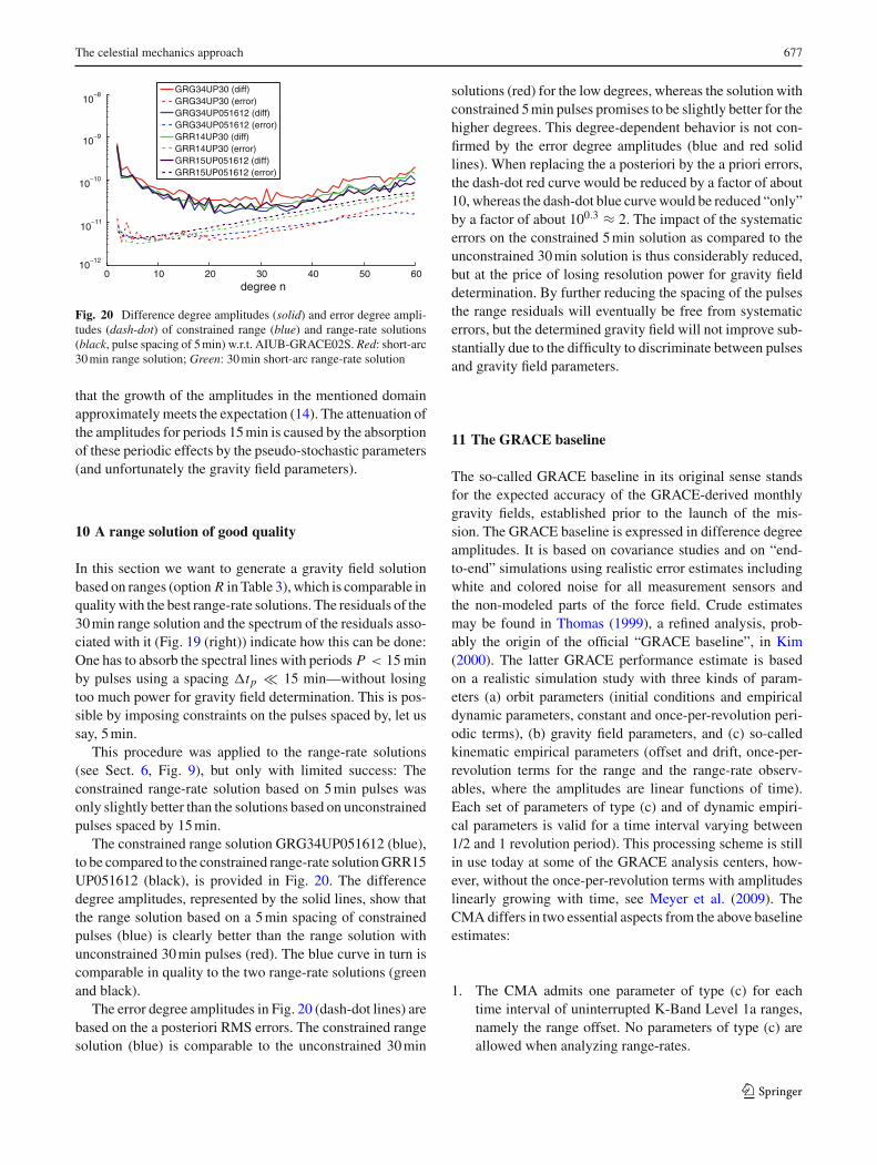
Fig. 20 Difference degree amplitudes (solid) and error degree ampli-tudes (dash-dot) of constrained range (blue) and range-rate solutions(black, pulse spacing of 5 min) w.r.t. AIUB-GRACE02S. Red: short-arc30 min range solution; Green: 30 min short-arc range-rate solution

that the growth of the amplitudes in the mentioned domainapproximately meets the expectation (14). The attenuation ofthe amplitudes for periods 15 min is caused by the absorptionof these periodic effects by the pseudo-stochastic parameters(and unfortunately the gravity field parameters).

10 A range solution of good quality

In this section we want to generate a gravity field solutionbased on ranges (option R in Table 3), which is comparable inquality with the best range-rate solutions. The residuals of the30 min range solution and the spectrum of the residuals asso-ciated with it (Fig. 19 (right)) indicate how this can be done:One has to absorb the spectral lines with periods P < 15 minby pulses using a spacing �tp 15 min—without losingtoo much power for gravity field determination. This is pos-sible by imposing constraints on the pulses spaced by, let ussay, 5 min.

This procedure was applied to the range-rate solutions(see Sect. 6, Fig. 9), but only with limited success: Theconstrained range-rate solution based on 5 min pulses wasonly slightly better than the solutions based on unconstrainedpulses spaced by 15 min.

The constrained range solution GRG34UP051612 (blue),to be compared to the constrained range-rate solution GRR15UP051612 (black), is provided in Fig. 20. The differencedegree amplitudes, represented by the solid lines, show thatthe range solution based on a 5 min spacing of constrainedpulses (blue) is clearly better than the range solution withunconstrained 30 min pulses (red). The blue curve in turn iscomparable in quality to the two range-rate solutions (greenand black).

The error degree amplitudes in Fig. 20 (dash-dot lines) arebased on the a posteriori RMS errors. The constrained rangesolution (blue) is comparable to the unconstrained 30 min

solutions (red) for the low degrees, whereas the solution withconstrained 5 min pulses promises to be slightly better for thehigher degrees. This degree-dependent behavior is not con-firmed by the error degree amplitudes (blue and red solidlines). When replacing the a posteriori by the a priori errors,the dash-dot red curve would be reduced by a factor of about10, whereas the dash-dot blue curve would be reduced “only”by a factor of about 100.3 ≈ 2. The impact of the systematicerrors on the constrained 5 min solution as compared to theunconstrained 30 min solution is thus considerably reduced,but at the price of losing resolution power for gravity fielddetermination. By further reducing the spacing of the pulsesthe range residuals will eventually be free from systematicerrors, but the determined gravity field will not improve sub-stantially due to the difficulty to discriminate between pulsesand gravity field parameters.

11 The GRACE baseline

The so-called GRACE baseline in its original sense standsfor the expected accuracy of the GRACE-derived monthlygravity fields, established prior to the launch of the mis-sion. The GRACE baseline is expressed in difference degreeamplitudes. It is based on covariance studies and on “end-to-end” simulations using realistic error estimates includingwhite and colored noise for all measurement sensors andthe non-modeled parts of the force field. Crude estimatesmay be found in Thomas (1999), a refined analysis, prob-ably the origin of the official “GRACE baseline”, in Kim(2000). The latter GRACE performance estimate is basedon a realistic simulation study with three kinds of param-eters (a) orbit parameters (initial conditions and empiricaldynamic parameters, constant and once-per-revolution peri-odic terms), (b) gravity field parameters, and (c) so-calledkinematic empirical parameters (offset and drift, once-per-revolution terms for the range and the range-rate observ-ables, where the amplitudes are linear functions of time).Each set of parameters of type (c) and of dynamic empiri-cal parameters is valid for a time interval varying between1/2 and 1 revolution period). This processing scheme is stillin use today at some of the GRACE analysis centers, how-ever, without the once-per-revolution terms with amplitudeslinearly growing with time, see Meyer et al. (2009). TheCMA differs in two essential aspects from the above baselineestimates:

1. The CMA admits one parameter of type (c) for eachtime interval of uninterrupted K-Band Level 1a ranges,namely the range offset. No parameters of type (c) areallowed when analyzing range-rates.

123


Table 4 CMA processingoptions for K-Band analysis Solution σapr/σpost Rel. constraint Characteristics

GRR14UP30 0.2/0.276 – Pulse spacing of 30 min, R R

GRR14UP15 0.2/0.249 – Pulse spacing of 15 min, R R

GRR14UP051612 0.2/0.322 1.0 × 10−8 m/s Pulse spacing of 5 min, R R

GRG34UP30 0.7/7.40 – Pulse spacing of 30 min, R

GRG34UP15 0.7/3.53 – Pulse spacing of 15 min, R

GRG34UP051612 0.7/1.87 1.0 × 10−8 m/s Pulse spacing of 5 min, R

0 10 20 30 40 50 6010

−6

10−5

10−4

10−3

degree n

m GRR14UP30 (a priori)GRR14UP30 (a posteriori)GRR14UP15 (a priori)GRR14UP15(a posteriori)GRR14UP051612 (a priori)GRR14UP051612(a posteriori)

0 10 20 30 40 50 6010

−6

10−5

10−4

10−3

10−2

degree nm

GRG34UP30 (a priori)GRG34UP30 (a posteriori)GRG34UP15 (a priori)GRR34UP15(a posteriori)GRG34UP051612 (a priori)GRR34UP051612(a posteriori)

Fig. 21 GRACE baselines, expressed in error degree amplitudes, for the solutions in Table 4; 30 days, geoid heights; left range-rate, right range

2. The CMA allows for the estimation of (constrained)pseudo-stochastic parameters, which have the capabil-ity to absorb the non-modeled parts of the force field.

From our perspective there is no justification for introducingother (than offset) parameters of type (c). Kim (2000) justi-fies the parameters of type (c) in essence with the white andcolored noise present in the accelerometer measurements orin the background models. The parameters of type (c) thusplay a similar role as the pseudo-stochastic parameters in theCMA. Both error sources do exist, but from our perspectivethey should be dealt with on the level they occur, i.e., theyshould be absorbed by empirical dynamic parameters or bypseudo-stochastic parameters. The constant accelerations inR, S, W , the once-per-revolution terms, and the pulses orthe piecewise constant accelerations assume this role in theCMA.

For these reasons it seems appropriate to generate CMA-specific “GRACE baselines”, also in terms of error degreeamplitudes, for the more important processing strategies dis-cussed previously. Two kinds of “baselines” are provided:Those based on the inverted NEQ-matrix multiplied by thea priori RMS of the observable and those based on the esti-mated covariance matrix.

As the classical GRACE baseline is usually referred todata spans of one month and is expressed in geoidal heights,the CMA-specific GRACE baselines are also provided ingeoidal heights (in m) referring to 30 days of data, bymultiplying the dimensionless error degree amplitudes by

ae × √50/30 ≈ 1.291 × ae, where ae = 6,378,137 m is the

equatorial radius of the Earth. This re-scaling gives slightlytoo optimistic values, as the effect of the improved geograph-ical coverage from 30 to 50 days is not taken into account.

Table 4 summarizes the six solutions, for which “base-lines” are provided. Three of them are based on range-rate(without correlations) and three on range (without correla-tions). Two solutions out of the three in each group are con-tiguous, but otherwise unconstrained short-arc solutions, theother one is based on constrained pulses (separated by 5 min).The constraints may also be found in Table 4. The base-lines are of a similar order of magnitude for range-rate andrange—if the covariance matrix is used to calculate the errordegree amplitudes (dash-dot curves). If the RMS a prioriis used for scaling the inverted NEQ matrix, the baselineswhich are derived from the range observable and which arebased on (comparatively) few pseudo-stochastic parameterspromise to be much better than the corresponding baselineusing the covariance matrix. This statement is best seen inFig. 21, red curves. The big difference of course only provesthat

• there are either substantial non-modeled systematics inthe force field not captured by the accelerometers (e.g.,errors in the background models describing temporalgravity field variations like tidal effects, de-aliasing prod-ucts);

• or that the accelerometers do not perform as they should;

123


0 10 20 30 40 50 6010−5

10−4

10−3

10−2

degree n

m

GRR14UP051612(diff)GRR14UP051612 (error)

0 10 20 30 40 50 6010−5

10−4

10−3

10−2

degree n

m

GRG34UP051612 (diff)GRG34UP051612 (error)

Fig. 22 GRACE baselines, expressed in error degree amplitudes, and corresponding difference degree amplitude w.r.t. AIUB-GRACE02S, leftrange-rate, right range

• or that additional information needed to calculate the cen-ter-of-mass to center-of-mass distance between the twosatellites is substantially wrong;

• or that the reduction of the observations (from the rawK-Band measurements to the Level 1a ranges) is notcorrect.

Figure 22 shows the difference degree amplitudes of the30 days 5 min constrained solution (range-rates (left), ranges(right)) w.r.t. the biennial solution AIUB-GRACE02S. Oneclearly sees a big discrepancy towards the low degrees,whereas the higher difference degree amplitudes follow thecurve for the error degree amplitudes quite well. There stillis a discrepancy corresponding to a factor varying between 3and 10 between the achieved and the expected accuracy forthe corresponding range solution in Fig. 22 (right). The miss-ing time-varying signal in the mean field model (e.g., due tohydrology) may be responsible for some of the discrepanciesin the region of the low degree harmonics.

12 Summary and conclusions

The CMA was applied to 50 days of GRACE data, namely,to DOY 50–99/2007. Orbit and gravity field determinationwere considered. The gravity fields were always based onthe full set of 50 days of data in 2007. The solutions differin the underlying observables, in the parametrization, and inthe constraints imposed on the estimated orbit and/or pseudo-stochastic parameters. No constraints were imposed on theestimated gravity field parameters. Only the spherical har-monics within the limits 2 ≤ n ≤ 60 were determined, theterms 61 ≤ n ≤ 150 were taken over from the solutionAIUB-GRACE02Sp, which is based on the entire year 2007of GRACE data.

Orbit determination was studied in Sect. 4. The RMS errora posteriori of the GPS L1 phase observations was found tobe about σph ≈ 2 mm in an orbit determination experimentusing only the kinematic positions (together with the epoch-specific weight matrix) as pseudo-observations. The RMS aposteriori of the K-Band range-rate observable was estab-lished by a “K-Band only” analysis as σkbd,rr ≈ 0.2 µm/s,implying that the correct weight ratio to combine the K-Bandrange-rate and GPS NEQs is σ 2

ph/σ 2kbd,rr ≈ 108 s2. This

ratio was used for orbit and gravity field determination in ouranalyses.

It is an open issue to be addressed in future why the bestconsistency of gravity fields determined by the CMA withthose of other GRACE analysis teams is achieved with aweight ratio σ 2

ph/σ 2kbd,rr ≈ 1010 s2, which considerably de-

weights the GPS contribution.Standard procedures for gravity field estimation were dis-

cussed in Sect. 5. GPS-only, K-Band-only, and combinedGPS and K-Band gravity fields were produced. All K-Bandcontributions used the option R R in Table 3. Pulses in R, S,and W with a spacing of either 30, or 15, or 5 min were setup in different solutions. No or only weak constraints (5 minsolution) were imposed on the pulses. The main findingswere:

• GPS-only gravity fields up to a maximum degree ofnmax ≈ 60 may be determined using a data span of50 days—adopting the terms above n = 60 from an apriori solution of good quality.

• The sectorial terms are much better determined by GPSthan the zonal terms. Actually, the sectorial terms aredetermined with GPS with an accuracy comparable tothat of K-Band-only solutions.

• K-Band-only solutions are based on an a priori orbit estab-lished with K-Band and GPS (in this sense the attribute

123


“K-Band-only” is not correct). All terms, except those oflow degree n � 5, are established with high accuracy.

In Sect. 6 it was shown that the R R-solution (Table 3) withstrongly constrained 5 min pulses is of comparable quality asthe 30 min pulse solution without constraints.

The impact of accelerometer data on gravity field deter-mination using option R R (Table 3) was studied in Sect. 7.The main findings are:

• Gravity fields of good quality may be established evenwithout using acclerometer data.

• The difference degree amplitudes w.r.t. AIUB-GRACE02S when using accelerometer data improve by a factorof about 1–2.

• The S component of accelerometer data has the largestimpact on the K-Band observables.

Alternatives to option R R (Table 3) were studied in Sect. 8.The key findings are:

• Options R R and RD (Table 3) are equivalent, providedthe statistical information is chosen according to Eqs. (7,8, 12).

• Options R and RC (Table 3) are equivalent, provided thestatistical information is chosen according to Eqs. (9, 11,12).

• Options R RC and RC , thus also R, (Table 3) are equiva-lent, provided the statistical information is chosen accord-ing to Eqs. (9, 11, 12)

In Sect. 9 the residuals of range and range-rate solutionswere analyzed. Systematic effects dominate the range solu-tion. It was shown that the use of accelerometer data hasa much larger impact on range residuals than on range-rateresiduals. The overall fit improves roughly by a factor of 2when using the accelerometer data (the gain is much smallerfor range-rate residuals). The residuals of ranges and range-rates were spectrally analyzed for the entire interval of50 days. For periods P < 15 min the spectrum is richlypopulated with terms of amplitudes of the order of 10−8 m/sfor range-rate, of the order of 10−6 m for ranges—indicatingthe presence of systematic accelerations not absorbed by theaccelerometers.

In Sect. 10 we eventually produced a solution based onranges (option R, Table 3), which is of comparable quality asthe best range-rate solutions presented here. Unfortunately,many constrained pulses spaced by 5 min had to be set up,what weakened the much higher potential of the range solu-tions to determine the gravity field.

In Sect. 11 the GRACE baseline, as achievable currentlyby the CMA, was established. When taking into account the

non-modeled and/or the stochastic part of the force-field thediscrepancy of the difference degree amplitudes w.r.t. AIUB-GRACE02 and the error degree amplitudes are small fordegrees n � 20 for option R R (Table 3), somewhat larger foroptions R and RC . The error degree amplitudes are clearlytoo optimistic for low degrees n � 10. More work, in partic-ular concerning the GPS contribution, is required.

Acknowledgements This work was supported by the Swiss NationalScience Foundation (project “gravity field determination using positionsof low Earth orbiters established with the GPS” with number 200020–117908) and by the Institute for Advanced Study (IAS) of the Techni-sche Universität München. Both contributions are gratefully acknowl-edged.

References

Bettadpur S (2007) GRACE 327-720 (CSR-GR-03-02) Gravity recov-ery and climate experiment product specification document (Rev4.5, February 20, 2007), Center for Space Research, the Universityof Texas at Austin

Beutler G, A Jäggi, U Meyer, L Mervart (2010) The celestialmechanics approach: theoretical foundations. J Geod. doi:10.1007/s00190-010-0401-7

Dach R, Hugentobler U, Meindl M, Fridez P (eds) (2007) The BerneseGPS Software Version 5.0, Astronomical Institute, University ofBern

Descartes R (1637) Discours de la methode Pour bien conduire sa rai-son, & chercher la verité dans les sciences, Plus la dioptriuve, lesmeteores, et la geometrie, Qui sont des essais de cete Methode. ALeyde, De l’Imprimerie de Ian Maire MDCXXXVII

Ditmar P, Klees R, Liu X (2007) Frequency-dependent data weight-ing in global gravity field modeling from satellite data contam-inated by non-stationary noise. J Geod 81: 81–96. doi:10.1007/s00190-006-0074-4

Förste C, Flechtner F, Schmidt R, Stubenvoll R, Rothacher M, Kusche J,Neumayer KH, Biancale R, Lemoine JM, Barthelmes F, BruinsmaS, König R, Meyer U (2008) EIGEN-GL05C—a new global com-bined high-resolution GRACE-based gravity field model of theGFZ-GRGS cooperation. Geophysical Research Abstracts, vol 10

Jäggi A (2007) Pseudo-stochastic orbit modeling of low earth satellitesusing the Global Positioning System. Geodätisch-geophysikali-sche Arbeiten in der Schweiz, Vol 73, Schweizerische GeodätischeKommission, Institut für Geodäsie und Photogrammetrie, Eidg.Technische Hochschule, Zürich

Jäggi A, Beutler G, Prange L, Meyer U, Mervart L, Dach R, RummelR, Gruber T (2009) Gravity field determination at AIUB: currentactivities. EGU General Assembly 2009, EGU2009-8714

Jäggi A, Beutler G, Meyer U, Mervart L, Prange L, Dach R (2010)AIUB-GRACE02S—status of GRACE gravity field recoveryusing the celestial mechanics approach. International Associationof Geodesy Symposium (accepted for publication)

Kim J (2000) Simulation study of a low-low satellite-to-satellite track-ing mission. Ph D Dissertation, The University of Texas at Austin,May 2000

Lemoine FG, Smith DE, Kunz L, Smith R, Pavlis NK, Klosko SM,Chinn DS, Torrence MH, Willamson RG, Cox CM, Rachlin KE,Wang YM, Kenyon SC, Salman R, Trimmer R, Rapp RH, NeremRS (1997) The development of the NASA GSFC and NIMA JointGeopotential Model. In: Segawa J, Fujimoto H, Okubo S (eds) IAGsymposia gravity, geoid and marine geodesy. Springer, Berlin, pp461–469

123

http://dx.doi.org/10.1007/s00190-010-0401-7

http://dx.doi.org/10.1007/s00190-010-0401-7

http://dx.doi.org/ 10.1007/s00190-006-0074-4

http://dx.doi.org/ 10.1007/s00190-006-0074-4


Meyer U, Flechtner F, Schmidt R, Frommknecht B (2009) A simula-tion study discussing the GRACE baseline accuracy. Internationalassociation of geodesy symposium (accepted for publication)

Prange L, Jäggi A, Beutler G, Mervart L, Dach R (2009) Gravity fielddetermination at the AIUB—the Celestial mechanics approach. In:Sideris MG (ed) Observing our changing Earth. Springer, Berlin,pp 353–362. doi:10.1007/978-3-540-85426-5-42

Prange L, Jäggi A, Bock H, Dach R (2010) The AIUB-CHAMP02Sand the influence of GNSS model changes on gravity field recov-ery using spaceborne GPS. Adv Space Res 45(2):215–224. doi:10.1016/j.asr.2009.09.020

Thomas J.B. (1999) An analysis of gravity-field estimation basedon intersatellite dual-1-way biased ranging. JPL Publica-tion 98-15 http://podaac.jpl.nasa.gov/pub/grace/doc/newsletters/GRACE_SDS_NL_0401.pdf

Touboul P, Willemenot E, Foulon B, Josselin V (1999) Accelerometersfor CHAMP, GRACE and GOCE space missions: synergy andevolution. Boll Geof Teor Appl 40:321-327

123

http://dx.doi.org/10.1007/978-3-540-85426-5-42

http://dx.doi.org/10.1016/j.asr.2009.09.020

http://dx.doi.org/10.1016/j.asr.2009.09.020

http://podaac.jpl.nasa.gov/pub/grace/doc/newsletters/GRACE_SDS_NL_0401.pdf

http://podaac.jpl.nasa.gov/pub/grace/doc/newsletters/GRACE_SDS_NL_0401.pdf

the celestial mechanics approach: application to data of

Documents