the chemical master equation in gene networks: complexity...
TRANSCRIPT

The Chemical Master Equation in Gene Networks: Complexity and Approaches
Mustafa Khammash
Center for Control, Dynamical-Systems, and ComputationsUniversity of California at Santa Barbara

Outline
• Gene expression
‣ An introduction
‣ Stochasticity in gene expression
‣ Randomness and variability
• Stochastic Chemical Kinetics
‣ The Chemical Master Equation (CME)
‣ Monte-Carlo simulations of the CME
• A new direct approach to solving the CME
‣ The Finite-State Projection Method
‣ Model reduction and aggregation
‣ Examples

Gene Expression
• An Introduction• Stochasticity in Gene Expression• Randomness and variability

Why Are Stochastic Models Needed?
• Much of the mathematical modeling of gene networks represents gene expression deterministically
• Deterministic models describe macroscopic behavior; but many cellular constituents are present in small numbers
• Considerable experimental evidence indicates that significant stochastic fluctuations are present
• There are many examples when deterministic models are not adequate

Modeling Gene Expression
Deterministic model
• Probability a single mRNA is transcribed intime dt is krdt.
• Probability a single mRNA is degraded intime dt is (#mRNA) · !rdt
Stochastic model
!p
kr
kp
!r
!
!
DNA
mRNA
protein

★ Deterministic steady-state equals stochastic mean ★ Coefficient of variation goes as 1/★ When mean is large, the coefficient of variation is (relatively) small
!
mean
Fluctuations at Small Copy Numbers
(mRNA)
(protein)
!p
kr
kp
!r
!
!
DNA
mRNA
protein
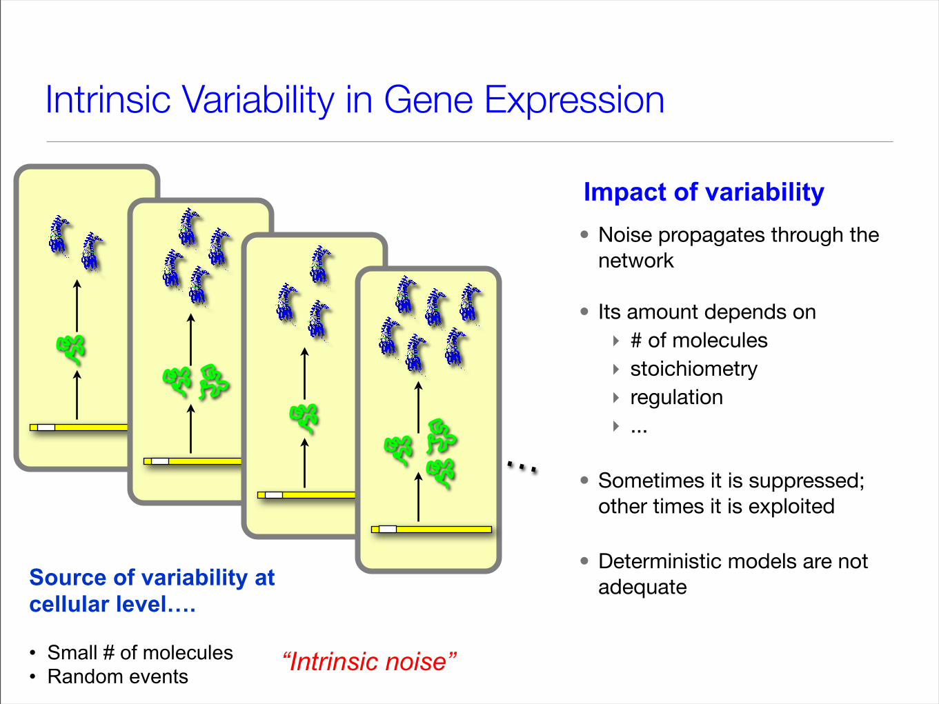
Intrinsic Variability in Gene Expression
• Noise propagates through the network
• Its amount depends on‣ # of molecules‣ stoichiometry‣ regulation ‣ ...
• Sometimes it is suppressed; other times it is exploited
• Deterministic models are not adequate
...
Source of variability at cellular level….
• Small # of molecules • Random events
“Intrinsic noise”
Impact of variability

Stochastic Influences on Phenotype
Fingerprints of identical twins Cc, the first cloned cat and her genetic mother
J. Raser and E. O’Shea, Science, 1995.

Exploiting the Noise
• Stochastic mean value different from deterministic steady state• Noise enhances signal!
Johan Paulsson , Otto G. Berg , and Måns Ehrenberg, PNAS 2000
stochastic
deterministic
0 10 20 30 40 50 60 70 80 90 10050
100
150
200
250
300
350
400
Time
Nu
mb
er o
f M
ole
cu
les
of
P

Noise Induced Oscillations
Circadian rhythm
Vilar, Kueh, Barkai, Leibler, PNAS 2002
• Oscillations disappear from deterministic model after a small reduction in deg. of repressor• (Coherence resonance) Regularity of noise induced oscillations can be manipulated by tuning the level of noise [El-Samad, Khammash]

The Pap Pili Stochastic Switch
• Pili enable uropathogenic E. coli to attach to epithelial cell receptors
‣ Plays an essential role in the pathogenesis of urinary tract infections
• E. coli expresses two states ON (piliated) or OFF (unpiliated)
• Piliation is controlled by a stochastic switch that involves random molecular events

A Simplified Pap Switch Model
Lrp
• Lrp can (un)bind either or both of two binding sites
• A (un)binding reaction is a random event
leucine regulatory protein
One gene g
Site 1 Site 2

R3R4
State g3
R8R7R6R5
State g4
R1 R2
Lrp
State g1
State g2

R3R4
State g3
R8R7R6R5
State g4
R1 R2
Lrp
State g1
State g2
PapI
ON
OFF
OFF
OFF
Piliation takes placeif gene is ON at specific
time: T

Identical Genotype Leads to Different Phenotype
genegene genegene
UnpiliatedPiliated
….

Stochastic Chemical Kinetics
• Mathematical Formulation• The Chemical Master Equation (CME)• Monte-Carlo Simulations of the CME

• The state of the system is described by the integer vector x = (x1, . . . , xn)T ;
xi is the population of species Si.
• (N-species) Start with a chemically reacting system containing N distinct
reacting species {S1, . . . , SN}.
population of S1
popula
tion
of
S2
Stochastic Chemical Kinetics

• (M-reactions) The system’s state
can change through any one of
M reaction: Rµ : µ ! {1,2, . . . , M}..
• (State transition) An Rµ re-
action causes a state transition
from x to x + sµ.
s1 =
!
1
0
"
; s2 =
!
0
!1
"
; s3 =
!
!1
0
"
1
2 3 4
56
7
8
R2 R1 R1 R2 R3 R2 R2Sequence:
popula
tion
of
S2
population of S1
S1 + S2 ! S1
! ! S1
S1 ! !R3
R2
R1Example:
Stoichiometry matrix:
S =!
s1 s2 . . . sM
"

• (Transition probability) Suppose the system is in state x.
The probability that Rµ is the next reaction and that it will occurs within
the next dt time units is given by aµ(x)dt.
If Rµ is the monomolecular reaction Si ! products, there exists some constant
cµ such that aµ(x) = cµxi.
cµ is numerically equal to the reaction rate constant kµ of conventional deter-
ministic chemical kinetics.
If Rµ is the bimolecular reaction Si + Sj ! products, there exists a constant cµ
such that aµ(x) = cµxixj.
cµ is equal to kµ/!, where kµ is the reaction rate constant, and ! is the
reaction volume

The Chemical Master Equation
The Chemical Master Equation (CME):

Challenges in the Solution of the CME
• The state space is potentially HUGE!
• Very often transitions have vastly different time-scales
•
N species
Up to n copies/species
Number of states: nN
! 104 di!erent proteins
! 106 copies/proteins (avg.)
! 106000 states!
Eukaryotic Cell
Proteins bind together to create even more species!
!a(x)! " # as !x! " #

For many species: n << 106
• Modularity: Small subsystems can often be isolated e.g. heat-shock has ~7 key interacting molecules
• Specificity: Each protein binds to one or very few other molecules
• Many “key” molecules exist in small numbers: genes, mRNAs, signaling and regulatory proteins, ... e.g. liver cells, 97% of mRNAs are present at ~10 copies/cell.
• Key molecules constitute many of the compound species: e.g. methylated DNA
Exploiting Underlying Biology
N << 104 N=23 (heat-shock) N=63 (pap switch)

• This approach constructs numerical realizations of x(t) and then histogram-
ming or averaging the results of many realizations (Gillespie 1976).
• At each SSA step: Based on this
distribution, the next reaction and the
time of its occurence are determined.
The state is updated.
Monte Carlo Simuations: The Stochastic Simulation Algorithm (SSA)
Px(!, µ) = aµ(x) exp
!
!
M"
j=1aj(x) !
#
,
• Start by computing the reaction probability density function Px(!, µ):
Px(!, µ) is the joint probability density function of the two random
variables:
– “time to the next reaction” (!);
– “index of the next reaction” (µ).
µ
τ
Px(τ,µ)
1
2
3
M dτ
...

An SSA run
popula
tion
of
S2
population of S1

SSA
• Low memory requirement
• In principle, computation does not depend exponentially on N
Advantages
Disadvantages• Can be very slow
• Convergence is slow
• No guaranteed error bounds
• Little insight
Computational e!ort =C1!2

A Direct Approach to the Chemical Master Equation
• The Finite State Projection Method• Model Reduction and Aggregation• Examples

The Chemical Master Equation (CME):
The states of the chemical system can be enumerated:
The probability density state vector is defined by:
The evolution of the probability density state vector is governed by

The Finite State Projection Approach
The probability density vectorevolves on an infinite integer lattice
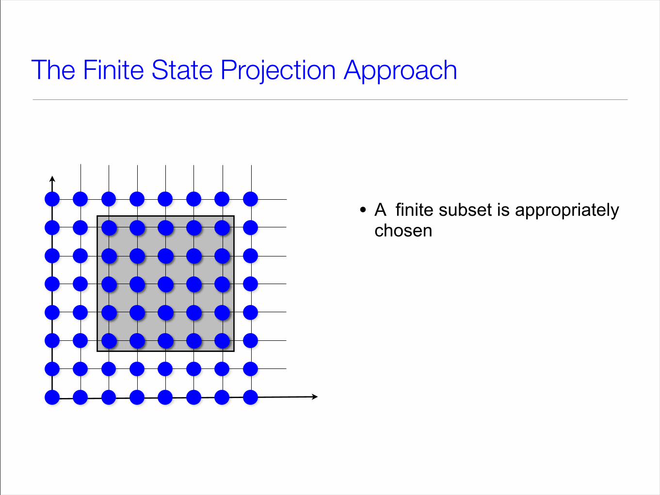
The Finite State Projection Approach
• A finite subset is appropriately chosen

The Finite State Projection Approach
• A finite subset is appropriately chosen
• The remaining (infinite) states are projected onto a single state (red)

The Finite State Projection Approach
The projected system can be solved exactly!
• A finite subset is appropriately chosen
• The remaining (infinite) states are projected onto a single state (red)
• Only transitions into removed states are retained
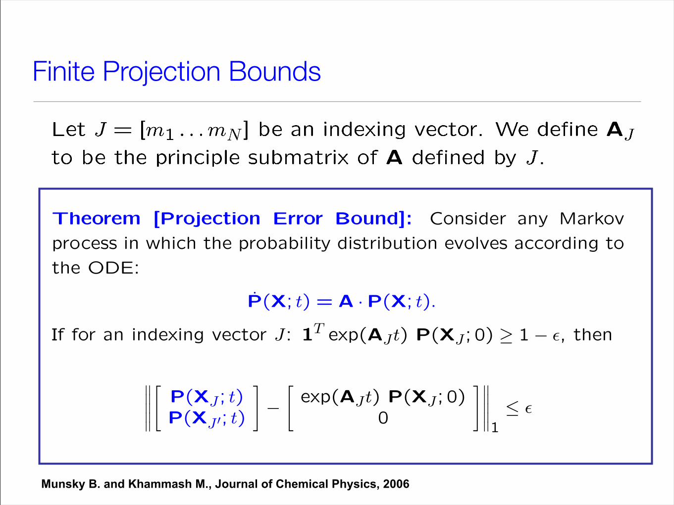
Finite Projection Bounds
Munsky B. and Khammash M., Journal of Chemical Physics, 2006
Theorem [Projection Error Bound]: Consider any Markov
process in which the probability distribution evolves according to
the ODE:
P(X; t) = A ·P(X; t).
If for an indexing vector J: 1T exp(AJt) P(XJ; 0) ! 1 " !, then
!
!
!
!
!
"
P(XJ; t)P(XJ #; t)
#
"
"
exp(AJt) P(XJ; 0)0
#!
!
!
!
!
1
$ !

The FSP Algorithm

Application to the Pap Switch Model
R1 R2 R3R4
R8R7R6R5
Lrp
PapI
State g3
State g4
State g1
State g2
ON
OFF
OFF
OFF
Piliation takes placeif gene is ON at a specific time: T
What is the probability of being in State g2 at time T?

Application to the Pap Switch Model
State g3
R1 R2R3 R4
R8R7R6R5
Lrp
PapI
State g4
State g1
State g2
An infinite number of states:
10 reactions

Application to the Pap Switch Model
A. Hernday and B. Braaten, and D. Low, “The Mechanism by which DNA Adenine Methylase and PapI Activate the Pap Epigenetic Switch,” Molecular Cell,vol. 12, 947-957, 2003.

Application to the Pap Switch Model
● Unlike Monte-Carlo methods (such as the SSA), the FSP directly approximates the solution of the CME.

Model Reduction and Time-Scale Separation

Reducing Unobservable Configurations
• Often one is not interested in the entire probability distribution. Instead one may wish only to estimate:
‣ a statistical summary of the distribution, e.g.
✴means, variances, or higher moments
‣ probability of certain traits:
✴switch rate, extinction, specific trajectories, etc…
• In each of these cases, one can define an output y:
• Frequently, the output of interest relates to small subset of the state space

Aggregation and Model Reduction
Given Generic CME in the form of a linear ODE:
P(X, t) = AP(X, t)
The system begins in the set U at time t = 0 with pdv: P(XU,0).

Aggregation and Model Reduction
The full pdv evolves according to:
• The unreachable states cannot be excited by reachable ones (may be removed!)
0 0
0 0
• The unobservable states may not excite the observable ones
The full system reduces to:!
P(XRO, t)P(XRO!, t)
"
=
!
ARO,RO 0
ARO!,RO ARO!,RO!
" !
P(XRO, t)P(XRO!, t)
"
!
P(XRO, t)1T P(XRO!, t)
"
=
!
ARO,RO 0
1TARO!,RO 1TARO!,RO!
" !
P(XRO, t)P(XRO!, t)
"
We need only keep track of the dynamics of unobservable states as a whole
0
0 00

Begin with a full integer lattice description of the system
FSP: Aggregation and Model Reduction

Remove unreachable states and aggregate unobservable ones
FSP: Aggregation and Model Reduction

Project the remaining states onto a finite subset
FSP: Aggregation and Model Reduction

Reduction Through Time-Scale Separation
• It often occurs in chemical systems that some reactions are very fast, while others are relatively slow
• These differences in reaction rates lead to significant numerical stiffness
• Often the fast dynamics are not of interest
• One may remove the fast dynamics and focus on the dynamics on the slow manifold

Group together states that
are connected through fast
transitions
Fast groups reach proba-
bilistic equilibrium before a
slow transition occurs
Aggregate fast group into
states
Transition propensity is the
weighted sum of transition
propensities of unaggregated
states
Time Scale Separation
popula
tion
of
S2
population of S1

• Each Hi is a generator for a fast group of states. !L is the slow
coupling reactions between blocks.
• Each Hi has a single zero eigenvalue, " = 0, the rest of the eigen-
values have large negative real parts.
• Each Hi has a right eigenvector, vi , and a left eigenvector, 1T that
correspond to the zero eigenvalue.
Time Scale Separation
P =
!
"
"
"
#
$
%
%
%
&
H1 0
0 H2. . .
. . . . . .. . . Hm
'
(
(
(
)
+ !L
*
+
+
+
,
P
U =
!
"
"
"
"
#
1T 0
0 1T . . .
. . .. . .
. . . 1T
$
%
%
%
%
&
V =
!
"
"
"
#
v1 0
0 v2. . .
. . . . . .. . . vm
$
%
%
%
&
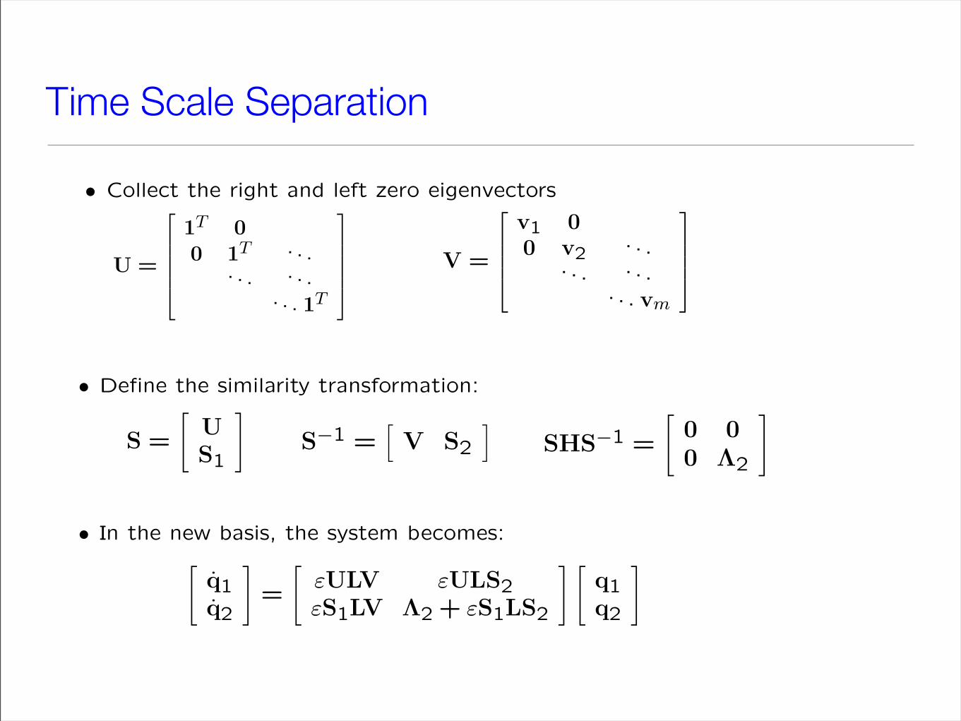
• Collect the right and left zero eigenvectors
S!1 =
!
V S2
"
SHS!1 =
!
0 0
0 !2
"
S =
!
U
S1
"
• Define the similarity transformation:
!
q1
q2
"
=
!
!ULV !ULS2
!S1LV !2 + !S1LS2
" !
q1
q2
"
• In the new basis, the system becomes:
Time Scale Separation

• Ignoring the fast stable modes, the dynamics of q1
q1 ! !ULVq1
P(t) ! !V exp(ULVt)UP(0)
• In the original coordinate system, P (t) is given by
• Note that only the zero eigenvectors of Hi need to be computed!
Simon HA, Ando A. Aggregation of variables in dynamic systems. Econometrica 1961; 29(2):111–138.
Phillips RG, and Kokotovic P, A Singular perturbation approach to modeling and control of Markov Chains,IEEE Transactions on Automatic Control, 26 (5): 1087-1094, 1981.
Time Scale Separation
!
q1
q2
"
=
!
!ULV !ULS2
!S1LV !2 + !S1LS2
" !
q1
q2
"

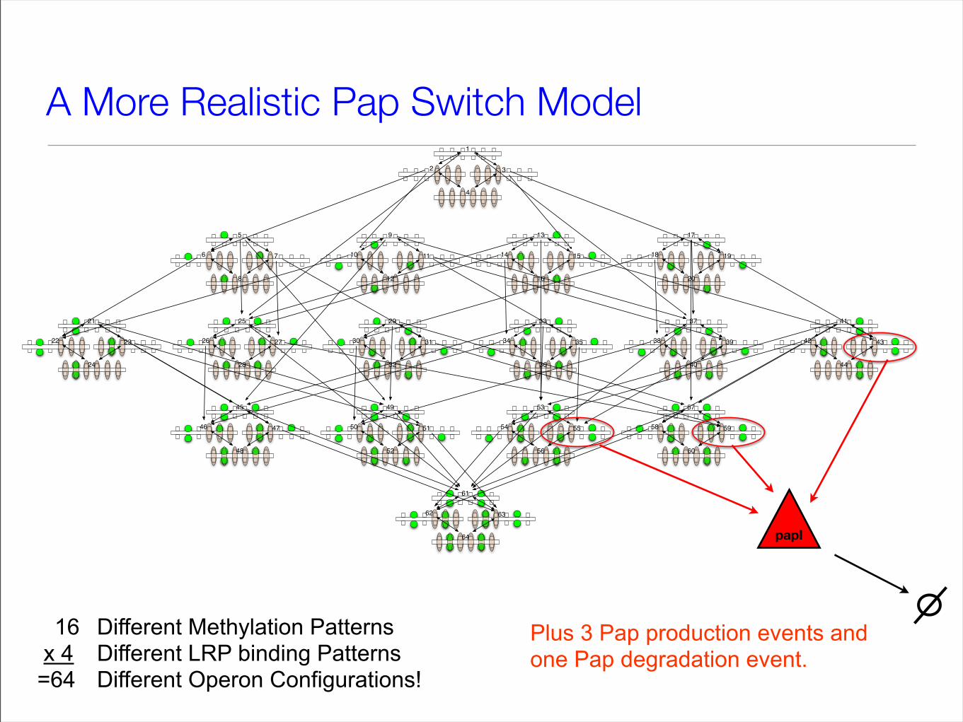
Example: The Full Pap Switch Model

A More Realistic Pap Switch Model
1
2
3
4
Lrp
4 gene states based on Lrp binding sites

1
2 3 4 5
6 7 8 9 10 11
12 13 14 15
16
CH3
A More Realistic Pap Switch Model
16 different possible methylation patterns
DNA Adenine Methylase (DAM) can methylate the gene at the
GATC site

1
4
2 3
9
12
10 11
5
8
6 7
17
20
18 19
13
16
14 15
45
48
46 47
49
52
50 51
53
56
54 55
57
60
58 59
61
64
62 63
25
28
26 27
29
32
30 31
33
36
34 35
37
40
38 39
41
44
42 43
21
24
22 23
A More Realistic Pap Switch Model
1
4
2 3
9
12
10 11
5
8
6 7
17
20
18 19
13
16
14 15
45
48
46 47
49
52
50 51
53
56
54 55
57
60
58 59
61
64
62 63
25
28
26 27
29
32
30 31
33
36
34 35
37
40
38 39
41
44
42 43
21
24
22 23
16 Different Methylation Patterns x 4 Different LRP binding Patterns =64 Different Operon Configurations!
Plus 3 Pap production events and one Pap degradation event.
papI
A More Realistic Pap Switch Model

1
4
2 3
9
12
10 11
5
8
6 7
17
20
18 19
13
16
14 15
45
48
46 47
49
52
50 51
53
56
54 55
57
60
58 59
61
64
62 63
25
28
26 27
29
32
30 31
33
36
34 35
37
40
38 39
41
44
42 43
21
24
22 23
16 Different Methylation Patterns x 4 Different LRP binding Patterns =64 Different Operon Configurations!
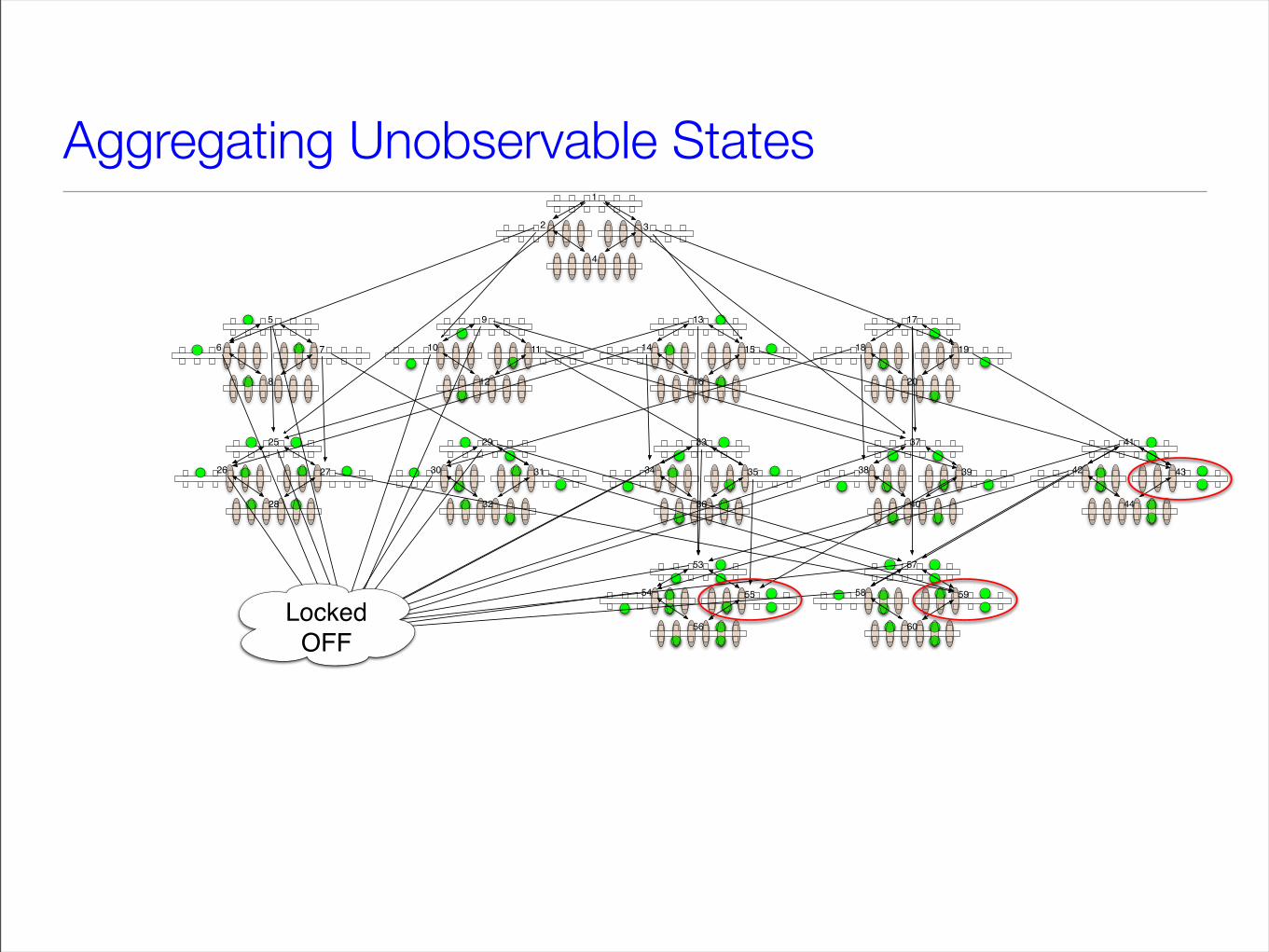
Locked OFF States
These States are unobservable from the ON states and can be aggregated.
Aggregating Unobservable States
1
4
2 3
9
12
10 11
5
8
6 7
17
20
18 19
13
16
14 15
53
56
54 55
57
60
58 59
25
28
26 27
29
32
30 31
33
36
34 35
37
40
38 39
41
44
42 43
4
54
8
4
6
4
7
4
95
2
5
0
5
1
6
16
4
6
2
6
3
2
12
4
2
2
2
3
Locked
OFF
Aggregating Unobservable States

Aggregating Fast States
2
1
3 4 5
6 7 8 9
11 12
10

Table 1: A comparison of the e!ciency and accuracy of the FSP, SSA, andapproximate FSP and SSA methods.Method # Simulations Time (s)a Relative Errorb
Full Model
FSP N.A. c 42.1 < 0.013%SSA 104 > 150 days Not available
Reduced Model
FSP approx. N.A. 3.3 ! 1.3%SSA approx. 104 9.8 ! 16%SSA approx. 105 94.9 ! 7.7%SSA approx. 106 946.2 ! 1.6%
aAll computations have been performed in Matlab 7.2on a 2.0 MHz PowerPC G5.
bError in switch rate is computed at t = 4000scThe FSP is run only once with a specified allowable
total error of 10!5.
FSP vs. Monte Carlo Algorithms

Reduced FSPQS−SSA (104 runs)QS−SSA (105 runs)QS−SSA (106 runs)
Comparisons
0 2000 4000 6000 8000 100000
0.2
0.4
0.6
0.8
1
1.2
1.4
1.6x 10⁻³
Time (s)
Full FSP
Pro
babi
lity
of O
N S
tate

Conclusions
• Low copy numbers of important cellular components give rise to stochasticity in gene expression. This in turn results in cell-cell variations.
• Organisms use stochasticity to their advantage
• Stochastic modeling and computation is an emerging area in Systems Biology
• New tools are being developed. More are needed.
• Many challenges and opportunities for control and system theorists.

Acknowledgments
• Brian Munsky, UCSB
• David Low, UCSB
• Slaven Peles, UCSB

Prediction vs. Experiments

Moment Computations

The Linear Propensity Case