the classical monetary model - crei...2016/07/01 · the classical monetary model jordi galí crei,...
TRANSCRIPT

The Classical Monetary Model
Jordi Galí
CREI, UPF and Barcelona GSE
January 2019
Jordi Galí (CREI, UPF and Barcelona GSE) Classical Monetary Model January 2019 1 / 23

Assumptions
Perfect competition in goods and labor markets
Flexible prices and wages
Representative household
Money in the utility function
No capital accumulation
No fiscal sector
Closed economy
Jordi Galí (CREI, UPF and Barcelona GSE) Classical Monetary Model January 2019 2 / 23
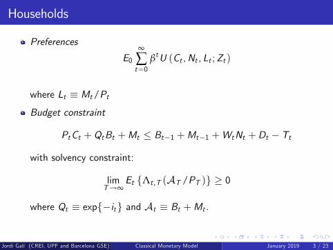
Households
Preferences
E0∞
∑t=0
βtU (Ct ,Nt , Lt ;Zt )
where Lt ≡ Mt/Pt
Budget constraint
PtCt +QtBt +Mt ≤ Bt−1 +Mt−1 +WtNt +Dt − Tt
with solvency constraint:
limT→∞
Et {Λt ,T (AT /PT )} ≥ 0
where Qt ≡ exp{−it} and At ≡ Bt +Mt .
Jordi Galí (CREI, UPF and Barcelona GSE) Classical Monetary Model January 2019 3 / 23
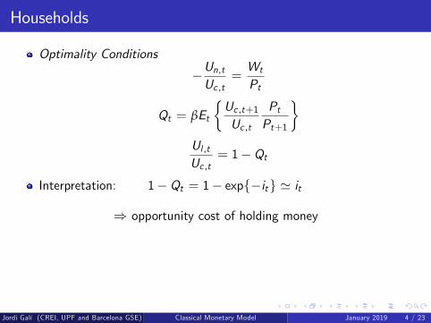
Households
Optimality Conditions
−Un,tUc ,t
=Wt
Pt
Qt = βEt
{Uc ,t+1Uc ,t
PtPt+1
}Ul ,tUc ,t
= 1−Qt
Interpretation: 1−Qt = 1− exp{−it} ' it
⇒ opportunity cost of holding money
Jordi Galí (CREI, UPF and Barcelona GSE) Classical Monetary Model January 2019 4 / 23
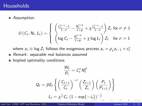
Households
Assumption:
U (Ct ,Nt , Lt ) =
(C 1−σt −11−σ − N 1+ϕ
t1+ϕ + χ L
1−σt −11−σ
)Zt for σ 6= 1(
logCt − N 1+ϕt1+ϕ + χ log Lt
)Zt for σ = 1
where zt ≡ logZt follows the exogenous process zt = ρzzt−1 + εztRemark : separable real balances assumedImplied optimality conditions
Wt
Pt= C σ
t Nϕt
Qt = βEt
{(Ct+1Ct
)−σ (Zt+1Zt
)(PtPt+1
)}Lt = χ
1σCt (1− exp{−it})−
1σ
Jordi Galí (CREI, UPF and Barcelona GSE) Classical Monetary Model January 2019 5 / 23
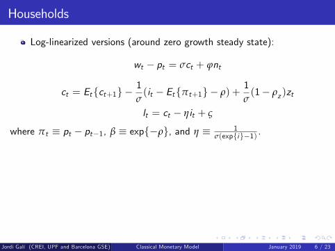
Households
Log-linearized versions (around zero growth steady state):
wt − pt = σct + ϕnt
ct = Et{ct+1} −1σ(it − Et{πt+1} − ρ) +
1σ(1− ρz )zt
lt = ct − ηit + ς
where πt ≡ pt − pt−1, β ≡ exp{−ρ}, and η ≡ 1σ(exp{i}−1) .
Jordi Galí (CREI, UPF and Barcelona GSE) Classical Monetary Model January 2019 6 / 23
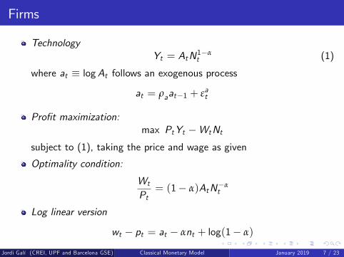
Firms
TechnologyYt = AtN1−α
t (1)
where at ≡ logAt follows an exogenous process
at = ρaat−1 + εat
Profit maximization:max PtYt −WtNt
subject to (1), taking the price and wage as given
Optimality condition:
Wt
Pt= (1− α)AtN−α
t
Log linear version
wt − pt = at − αnt + log(1− α)
Jordi Galí (CREI, UPF and Barcelona GSE) Classical Monetary Model January 2019 7 / 23

Policy
Government budget constraint
PtGt + BGt−1 = Tt +QtBGt + ∆MS
t
Fiscal policy: rule determining {Gt ,BGt ,Tt}Monetary policy: rule determining {MS
t , it}
Jordi Galí (CREI, UPF and Barcelona GSE) Classical Monetary Model January 2019 8 / 23
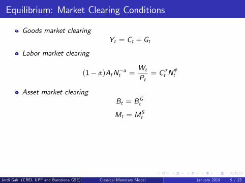
Equilibrium: Market Clearing Conditions
Goods market clearingYt = Ct + Gt
Labor market clearing
(1− α)AtN−αt =
Wt
Pt= C σ
t Nϕt
Asset market clearingBt = BGt
Mt = MSt
Jordi Galí (CREI, UPF and Barcelona GSE) Classical Monetary Model January 2019 9 / 23
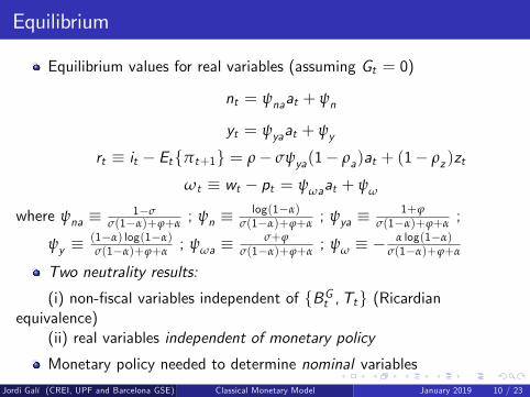
Equilibrium
Equilibrium values for real variables (assuming Gt = 0)
nt = ψnaat + ψn
yt = ψyaat + ψy
rt ≡ it − Et{πt+1} = ρ− σψya(1− ρa)at + (1− ρz )zt
ωt ≡ wt − pt = ψωaat + ψω
where ψna ≡ 1−σσ(1−α)+ϕ+α
; ψn ≡log(1−α)
σ(1−α)+ϕ+α; ψya ≡
1+ϕσ(1−α)+ϕ+α
;
ψy ≡(1−α) log(1−α)σ(1−α)+ϕ+α
; ψωa ≡σ+ϕ
σ(1−α)+ϕ+α; ψω ≡ −
α log(1−α)σ(1−α)+ϕ+α
Two neutrality results:
(i) non-fiscal variables independent of {BGt ,Tt} (Ricardianequivalence)
(ii) real variables independent of monetary policy
Monetary policy needed to determine nominal variables
Jordi Galí (CREI, UPF and Barcelona GSE) Classical Monetary Model January 2019 10 / 23
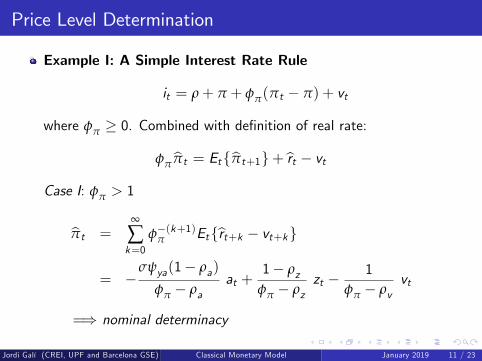
Price Level Determination
Example I: A Simple Interest Rate Rule
it = ρ+ π + φπ(πt − π) + vt
where φπ ≥ 0. Combined with definition of real rate:
φππ̂t = Et{π̂t+1}+ r̂t − vt
Case I: φπ > 1
π̂t =∞
∑k=0
φ−(k+1)π Et{r̂t+k − vt+k}
= −σψya(1− ρa)
φπ − ρaat +
1− ρzφπ − ρz
zt −1
φπ − ρvvt
=⇒ nominal determinacy
Jordi Galí (CREI, UPF and Barcelona GSE) Classical Monetary Model January 2019 11 / 23
Price Level Determination
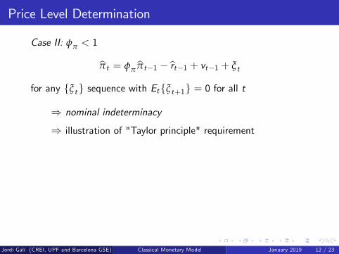
Case II: φπ < 1
π̂t = φππ̂t−1 − r̂t−1 + vt−1 + ξt
for any {ξt} sequence with Et{ξt+1} = 0 for all t
⇒ nominal indeterminacy
⇒ illustration of "Taylor principle" requirement
Jordi Galí (CREI, UPF and Barcelona GSE) Classical Monetary Model January 2019 12 / 23
Price Level Determination
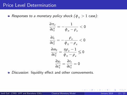
Responses to a monetary policy shock (φπ > 1 case):
∂πt∂εvt
= − 1φπ − ρv
< 0
∂it∂εvt
= − ρvφπ − ρv
< 0
∂mt∂εvt
=ηρv − 1φπ − ρv
≶ 0
∂yt∂εvt
=∂rt∂εvt
= 0
Discussion: liquidity effect and other comovements.
Jordi Galí (CREI, UPF and Barcelona GSE) Classical Monetary Model January 2019 13 / 23
Price Level Determination
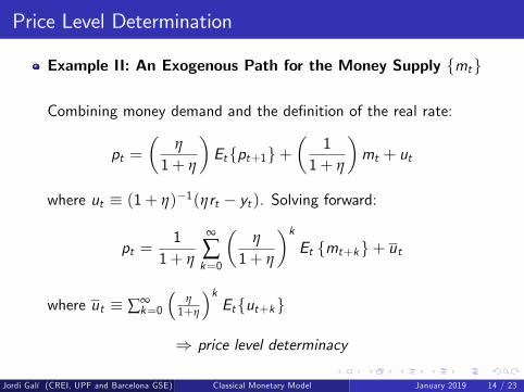
Example II: An Exogenous Path for the Money Supply {mt}
Combining money demand and the definition of the real rate:
pt =(
η
1+ η
)Et{pt+1}+
(1
1+ η
)mt + ut
where ut ≡ (1+ η)−1(ηrt − yt ). Solving forward:
pt =1
1+ η
∞
∑k=0
(η
1+ η
)kEt {mt+k}+ ut
where ut ≡ ∑∞k=0
(η1+η
)kEt{ut+k}
⇒ price level determinacy
Jordi Galí (CREI, UPF and Barcelona GSE) Classical Monetary Model January 2019 14 / 23
Price Level Determination
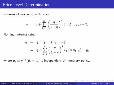
In terms of money growth rates:
pt = mt +∞
∑k=1
(η
1+ η
)kEt {∆mt+k}+ ut
Nominal interest rate:
it = η−1 (yt − (mt − pt ))
= η−1∞
∑k=1
(η
1+ η
)kEt {∆mt+k}+ ut
where ut ≡ η−1(ut + yt ) is independent of monetary policy.
Jordi Galí (CREI, UPF and Barcelona GSE) Classical Monetary Model January 2019 15 / 23
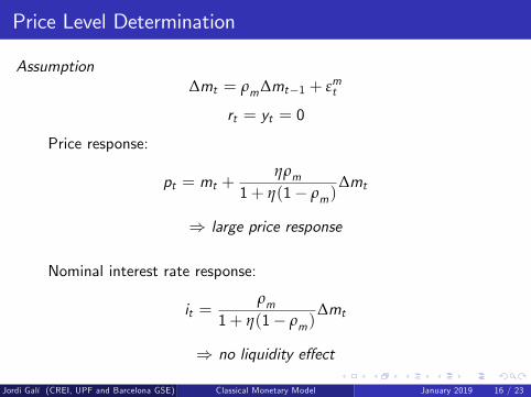
Price Level Determination
Assumption∆mt = ρm∆mt−1 + εmt
rt = yt = 0
Price response:
pt = mt +ηρm
1+ η(1− ρm)∆mt
⇒ large price response
Nominal interest rate response:
it =ρm
1+ η(1− ρm)∆mt
⇒ no liquidity effect
Jordi Galí (CREI, UPF and Barcelona GSE) Classical Monetary Model January 2019 16 / 23
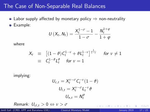
The Case of Non-Separable Real Balances
Labor supply affected by monetary policy ⇒ non-neutralityExample:
U (Xt ,Nt ) =X 1−σt − 11− σ
− N1+ϕt
1+ ϕ
where
Xt ≡[(1− ϑ)C 1−ν
t + ϑL1−νt
] 11−v for ν 6= 1
≡ C 1−ϑt Lϑ
t for ν = 1
implying:Uc ,t = X ν−σ
t C−νt (1− ϑ)
Ul ,t = Xν−σt L−ν
t ϑ
Un,t = Nϕt
Remark: Ucl ,t > 0 ⇔ ν > σJordi Galí (CREI, UPF and Barcelona GSE) Classical Monetary Model January 2019 17 / 23
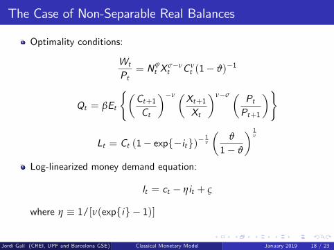
The Case of Non-Separable Real Balances
Optimality conditions:
Wt
Pt= Nϕ
t Xσ−νt C ν
t (1− ϑ)−1
Qt = βEt
{(Ct+1Ct
)−ν (Xt+1Xt
)ν−σ ( PtPt+1
)}
Lt = Ct (1− exp{−it})−1ν
(ϑ
1− ϑ
) 1ν
Log-linearized money demand equation:
lt = ct − ηit + ς
where η ≡ 1/[ν(exp{i} − 1)]
Jordi Galí (CREI, UPF and Barcelona GSE) Classical Monetary Model January 2019 18 / 23
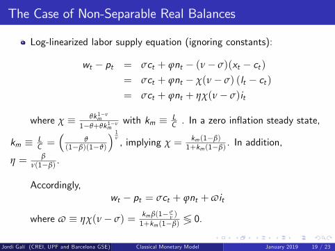
The Case of Non-Separable Real Balances
Log-linearized labor supply equation (ignoring constants):
wt − pt = σct + ϕnt − (ν− σ)(xt − ct )= σct + ϕnt − χ(ν− σ) (lt − ct )= σct + ϕnt + ηχ(ν− σ)it
where χ ≡ θk 1−νm
1−θ+θk 1−νm
with km ≡ LC . In a zero inflation steady state,
km ≡ LC =
(ϑ
(1−β)(1−ϑ)
) 1ν, implying χ = km (1−β)
1+km (1−β). In addition,
η = βν(1−β)
.
Accordingly,wt − pt = σct + ϕnt +vit
where v ≡ ηχ(ν− σ) =kmβ(1− σ
ν )1+km (1−β)
≶ 0.
Jordi Galí (CREI, UPF and Barcelona GSE) Classical Monetary Model January 2019 19 / 23
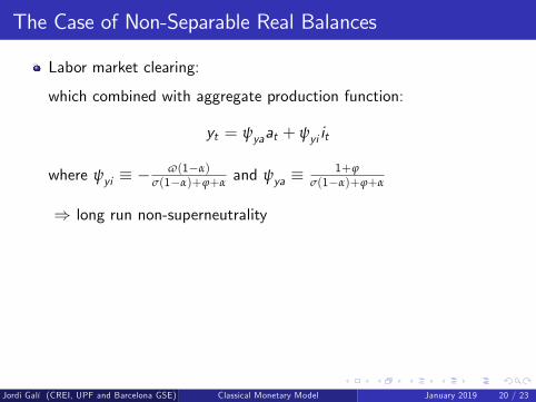
The Case of Non-Separable Real Balances
Labor market clearing:
which combined with aggregate production function:
yt = ψyaat + ψyi it
where ψyi ≡ −v(1−α)
σ(1−α)+ϕ+αand ψya ≡
1+ϕσ(1−α)+ϕ+α
⇒ long run non-superneutrality
Jordi Galí (CREI, UPF and Barcelona GSE) Classical Monetary Model January 2019 20 / 23
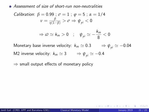
Assessment of size of short-run non-neutralities
Calibration: β = 0.99 ; σ = 1 ; ϕ = 5 ; α = 1/4ν = β
η(1−β)> σ ⇒ ψyi < 0
⇒ v ' km > 0 ; ψyi ' −km8< 0
Monetary base inverse velocity: km ' 0.3 ⇒ ψyi ' −0.04M2 inverse velocity: km ' 3 ⇒ ψyi ' −0.4
⇒ small output effects of monetary policy
Jordi Galí (CREI, UPF and Barcelona GSE) Classical Monetary Model January 2019 21 / 23
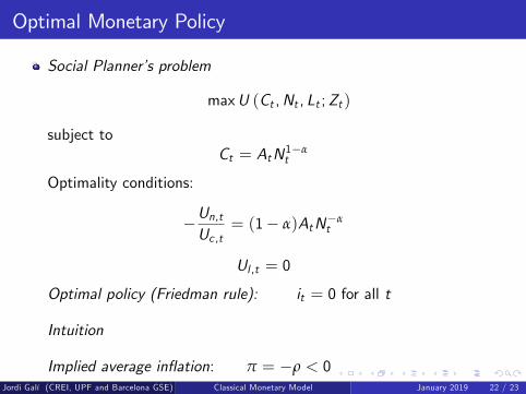
Optimal Monetary Policy
Social Planner’s problem
maxU (Ct ,Nt , Lt ;Zt )
subject toCt = AtN1−α
t
Optimality conditions:
−Un,tUc ,t
= (1− α)AtN−αt
Ul ,t = 0
Optimal policy (Friedman rule): it = 0 for all t
Intuition
Implied average inflation: π = −ρ < 0Jordi Galí (CREI, UPF and Barcelona GSE) Classical Monetary Model January 2019 22 / 23
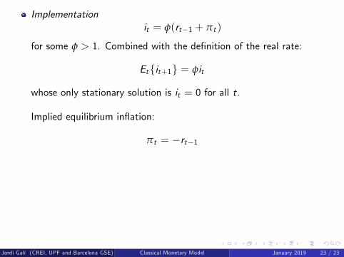
Implementationit = φ(rt−1 + πt )
for some φ > 1. Combined with the definition of the real rate:
Et{it+1} = φit
whose only stationary solution is it = 0 for all t.
Implied equilibrium inflation:
πt = −rt−1
Jordi Galí (CREI, UPF and Barcelona GSE) Classical Monetary Model January 2019 23 / 23