the cohesion system of hermin country and regional models
TRANSCRIPT

1
The COHESION System of HERMIN country and regional models:
Description and operating manual
Version 3
Contract no. 2005 CE 16 0 AT 027
prepared by
John Bradley Gerhard Untiedt
Muenster, September 2008
Contacts for communications GEFRA – Gesellschaft für Finanz- und Regionalanalysen Dr. Gerhard Untiedt Ludgeristr. 56, 48143 Münster, Germany, Phone: +49-251-2 63 93 11 Fax: +49-251-2 63 93 19 Mail: [email protected] Homepage: www.gefra-muenster.de EMDS - Economic Modelling and Development Strategies Dr. John Bradley 14 Bloomfield Avenue, Dublin 8, Ireland Phone: +353-1-454 5138 Fax: +353-1-497 0001 Mail: [email protected]

2
List of contributors
János Gács (Institute of Economics, Hungarian Academy of Sciences, Budapest)
Valentin Chavdarov and Lyubomir Dimitrov (Agency for Economic Analysis and Forecasting – AEAF, Sofia)
Timo Mitze (Gesellschaft für Finanz- und Regionalanalysen - GEFRA, Münster)
Janusz Zaleski and Pawel Tomascewski (Wrocławska Agencja Rozwoju Regionalnego S.A. - WARR, Wroclaw)
Manuela Unguru (Institute of World Economy, Romanian Academy)

3
Table of Contents
[1] GENERAL INTRODUCTION TO THE COHESION SYSTEM 8
1.1 Introductory remarks 8
1.2 Background context to the COHESION model system 8
1.3 Desirable features of the model system 9
1.4 Structure and organization of the User Manual 12
PART I 14
THE COHESION SYSTEM: A THEORETICAL DESCRIPTION 14
[2] COHESION SYSTEM: ORGANISATION AND SCOPE 15
2.1 Introduction 15
2.2 COHESION System: A model system or a system of models? 16
2.3 Historical data for the international environment 18
2.4 Medium-term forecasts for the international environment 18
[3] THE HERMIN COUNTRY MODELS: THEORETICAL STRUCTURE 20
3.1 Introductory remarks 20
3.2 Approaches to policy modelling 21
3.3 One-sector and two-sector small-open-economy frameworks 22
3.4 The structure of a HERMIN model 23
3.5 The supply side of the HERMIN model 26 3.5.1 Output determination 26 3.5.2 Factor demands 27 3.5.3 Sectoral wage determination 29 3.5.4 Demographics and labour supply 32
3.6 Absorption in HERMIN 33
3.7 National income in HERMIN 34 3.7.1 The public sector 34 3.7.2 The national income identities 34
3.8 The monetary sector 35 3.8.1 Introductory remarks 35 3.8.2 Types of monetary transmission mechanisms 37 3.8.3 Monetary experiments and monetary neutrality 38 3.8.4 Exchange rate patterns in cohesion countries 39

4
[4] TRANSMISSION MECHANISMS OF COHESION POLICIES 44
4.1 Introduction 44
4.2 Inserting the NSRF into the new model 44
4.3 Handling cohesion policy physical infrastructure impact analysis 48
4.4 Handling cohesion policy human resources impact analysis 50
4.5 Handling cohesion policy R&D impact analysis 53
4.6 Implications for equations in HERMIN 55 4.6.1 Manufacturing (T) sector effects: 55 4.6.2 Market Services (M) sector effects: 58 4.6.3 Building and Construction effects: 60 4.6.4 Agriculture (A) sector effects: 61 4.6.5 Non-market Services (G) sector effects: 62
PART II 63
CALIBRATING, TESTING AND USING THE 63
COHESION SYSTEM MODELS 63
[5] CALIBRATION OF THE BEHAVIOURAL EQUATIONS 64
5.1 Introductory remarks 64
5.2 Calibration results for behavioural equations 67
5.3 Concluding remarks on calibration 82
[6] SELECTION OF SPILLOVER AND OTHER PARAMETERS 83
6.1 Introductory remarks 83
6.2 The role of infrastructure 83
6.3 Human Capital 95
6.4: Measuring human capital 96
6.5 The role of R&D 98
[7] FROM CP FINANCIAL TABLES TO CP INVESTMENT TYPES 99
[8] TESTING THE COHESION COUNTRY MODELS 103
8.1 Introduction 103
8.2 Checking the model structure 103
8.3 Shocking the model 104

5
8.3.1 A shock to world output (OWM) 105 8.3.2 A public employment shock (LG) 106 8.3.3 A shock to government investment (IGV) 107 8.3.4 A shock to all exogenous price levels 107 8.3.5 Conclusions on responses to shocks 108
[9] ISSUES IN CONSTRUCTING BASELINE PROJECTIONS 110
9.1 Introduction 110
9.2 Short-term forecasting 111
9.3 Issues in medium and long-term forecasting 113 9.3.1 The international environment 113 9.3.2 The domestic policy environment 114
9.4 A HERMIN-based medium-term forecasting methodology 116 9.4.1 Projections: external and policy assumptions 117
9.5 Concluding remarks on forecasting 119
[10] THE COHESION SYSTEM IN ACTION 121
10.1 Introductory remarks 121
10.2 Background to the Spring 2007 analysis 121
10.3 Technical assumptions made in the simulations 123
10.4 Overview of main results, Spring 2007 125
10.5 Comparison of Spring and Autumn 2007 results 131
ANNEX CHAPTER 10: CP IMPACT TABLES - SPRING 2007 ANALYSIS 134
PART III 149
INSTALLING THE COHESION SYSTEM 149
[11] COHESION SYSTEM SOFTWARE REQUIREMENTS 150
11.1 Introductory remarks 150
11.2 Using the COHESION System software in practice 151
[12] SETTING UP THE HERMIN COUNTRY MODEL DATABASES 158
[13] CALIBRATING THE MODEL BEHAVIOURAL EQUATIONS 162
[14] IMPLEMENTING, TESTING AND RUNNING THE MODELS 165

6
[15] DATA SOURCES AND DATA GENERATION 169
[16] CONCLUSIONS AND FUTURE WORK PROGRAMME 179
REFERENCES 181

7

8
[1] General introduction to the COHESION System
1.1 Introductory remarks The first fully operational version of the COHESION System of HERMIN models was implemented and documented in March, 2007. A revised and updated version was implemented in September, 2007. The purpose of this third (annual) revised version is two-fold. First, to review the earlier versions of the User Manual with a view to making them more “user friendly” and self contained. Since the COHESION System of HERMIN models consists of sixteen national models and three regional models, its operation by users who were not involved in its construction and testing is a daunting task. This revision of the User Manual is part of the process of making the model system easier to operate, and of assisting the user in the interpretation of the results ederived from the model. The second purpose of the present revision of the User Manual is to document changes that have been made in the COHESION System of models since September, 2007. As was the case of the previous revision, these changes fall into three main groups. One set of changes arise from continuing updates that were made by DG-ECFIN to their AMECO database system. They concern mainly the treatment by AMECO of national accounts by ISIC production branches. Following approaches made by the authors of the COHESION System, the AMECO team issued a revised AMECO database in 2007 that now permits the separate treatment of the market (M) and non-market (G) services branches. In the first version of the COHESION System database, this separation had to be carried out using the EUROSTAT ISIC 17-branch data, obtained directly from the EUROSTAT web site, and this greatly complicated the task of constructing the database. In addition, AMECO/EUROSTAT now provides enough data for the new EU member states – and for Bulgaria and Romania in particular – to permit adoption of AMECO as the primary source of data for all 16 country models. A very small number of variables are obtained from other sources, including from national Statistics Offices. Another set of changes relate to further “standardisation” of the calibration of the COHESION System model behavioural equations. The short data sample available for the new member states (NMS), and their rapid development and structural change, means that calibration of behavioural equations using standard econometric techniques is a hazardous, and almost impossible task. In this third version of the COHESION System we continue to adopt the approach of imposing a higher degree of “standardisation” on behavioural parameters in order to eliminate the possibilities of parameter values that may be distorted by large fluctuations in the data sample. Finally, we continue to include a set of monetary mechanisms to those models of countries that operate independent monetary policies, i.e., countries that are neither in the euro zone nor operate currency boards.
1.2 Background context to the COHESION model system Since the reform of the European Union’s policy for economic and social cohesion in the late 1980s, both the Commission and the national governments of states who receive investment aid have been faced with two separate but inter-related tasks.

9
The first task involves the design of integrated programmes of public investment that implement the EU cohesion policy and which are part financed by Structural Funds and Cohesion Funds, and co-financed out of domestic resources.1 The second task involves the evaluation of the impact of the investment programmes that implement cohesion policy, before (ex ante), during (mid-term) and after (ex post) their implementation. Since the late 1980s, the task of impact evaluation has been implemented in two different ways. The first – micro evaluation – examines likely impacts at a highly disaggregated level of individual projects, measures and groups of measures. The second – macro evaluation – takes place at a more aggregated level of Operational Programmes and/or at the level of the entire set of investment programmes that implements cohesion policy. For the macro stage of evaluation, disaggregation of the cohesion policy investment categories takes the form of three economic categories: physical infrastructure, human resources and direct aid to firms. At present, we analyse cohesion policy impacts in terms of these three economic categories. If a higher degree of disaggregation were desired (e.g., further disaggregation into different types of physical infrastructure), then the design of the country models in the COHESION System would have to be modified accordingly. The COHESION System of HERMIN models is an instrument that has been designed to analyse the macroeconomic and macro-sectoral impacts of cohesion policy. We use the term “instrument” here to designate a model system that has been tested and found robust enough that it can, after documentation, installing, and training, be passed on the staff of DG Regional Policy in the Commission. Progressive revisions and upgrades of the modelling system will be installed and made fully operational within DG-REGIO for the duration of the present contract. It should then be possible for the Commission staff to carry out fairly routine cohesion policy simulations. However, since these staff were not involved in the development of the model, at this stage they will not be expected to take over the full maintenance and upgrading of the model. This will remain a task for the contractors for the duration of the present contract. The three main goals of the present User Manual are as follows:
1. To describe in detail how that system database is updated each year as new AMECO revisions are made available by DG-ECFIN;
2. To describe how the behavioural equations can be re-estimated in the light of
data revisions by AMECO;
3. To describe how the COHESION System of models can be used to examine cohesion policy impacts.
1.3 Desirable features of the model system The COHESION System of country and regional models needs to be capable of simulating the quantitative impacts of cohesion policy actions on a range of macro-economic variables. In fact, when using the model in this way, the analysis of the 1 Terminology used to describe these programmes has changed over the years. For the rest of the paper we will simply refer to “cohesion policy”, and the funds that are made available by the EU to implement these policies. We will use the term “cohesion policy” to embrace Structural Funds (ERDF, ESF, etc.) and Cohesion Funds (i.e., funds targeted at very specific kinds of physical infrastructure).

10
impacts on all the “endogenous” variables is possible. But in practice, users are normally only interested in the impacts on a small subset of important variables. The following is a specific list of target variables that are particularly relevant to macro analysis of cohesion policy: (i) Real GDP on an expenditure basis, and its standard components (private and
public consumption, investment, stock changes, exports and imports) (ii) Labour productivity, at the aggregate and branch levels; (iii) Employment in aggregate and by branch, and unemployment; (iv) Real and nominal wage rates, by branch; (v) Real and nominal interest rates and exchange rates; (vi) Inflationary consequences of cohesion policy (i.e., on wages and prices); (vii) The state of public finances (e.g., public sector deficits and debt
accumulation); (viii) Trade between receiving states and between receiving and net contributor
states; (ix) Labour migration between receiving states and between receiving and net
contributor states; (x) Development of different production branches (or sectors) of the economy,
and sectoral shifts; This list of “target” variables requires the support of a rather disaggregated and sophisticated model, and has some important implications for the design structure of the model, which we set out below. a) First, it implies that the model must have a fully articulated production,
expenditure and income side, permitting the quantification of cohesion policy impacts on a range of sectors and sectoral shifts (e.g., manufacturing, building and construction, agriculture, market and non-market services), on all the standard elements of expenditure, and on elements of income (such as wage rates and profit income).
b) Second, the model must have a fully articulated public sector revenue and
expenditure segment, to permit analysis of shifts in public sector balances due to the absorption and disbursement of EU funds.
c) Third, the model must have a carefully articulated labour market, distinguishing
labour demand (at level of sectors), labour supply (possibly distinguishing various types of labour), and population growth and migration.2
2 The focus on the labour market is justified since many of the important cohesion policy mechanisms are transmitted through the labour market (e.g., wage rates, competitiveness, productivity, etc.). Moreover, the Commission’s Community Strategic Guidelines for 2007-2013 make efforts to strengthen the synergies between the EU’s cohesion policies and the Lisbon Strategy by issuing guidelines, among others the comprehensive one: “More and better jobs”. Consequently, the analysis of cohesion policies requires special attention to be paid to modeling the labour market. More precisely, the labour market model should take into account the role of trade-unions, active labour market policies, labour market

11
d) Fourth, where necessary, the model should have monetary mechanisms in
order to permit analysis of the impact of cohesion policy on monetary variables (e.g., interest rates and exchange rates).
e) It must be possible to analyse the trade flows between individual receiving and
contributing countries in order to examine net trade impacts of cohesion policies.
f) The model should be structural, in the sense of being based, where necessary
and where appropriate on micro-foundations. Within that structure, the supply-side of the model must be designed in such a way as to permit incorporation of the main mechanisms through which cohesion policy impacts on the productive potential of a recipient economy.
The fact that most of the countries now receiving EU funds were previously centrally planned Communist states, and underwent a period of major transition to liberal market-based policies during the post-1989 period, means that it is not always possible to implement the complete set of the above modelling criteria. The COHESION System addresses many of the desired features, and background research will continue into the future. However, the kind of sophisticated econometric modelling that is common in the advanced, developed economies of the EU is unlikely to be feasible or appropriate for the new member states for some considerable time to come. Turning to the range of countries and macro-regions that are included in the COHESION System, these include regions and countries under the new Convergence objective and the countries eligible under the Cohesion Fund interventions. The coverage includes the following: (i) The ten new member states who joined the EU in 2004 (Estonia, Latvia,
Lithuania, Poland, the Czech Republic, Slovakia, Hungry, Slovenia, Malta and Cyprus);
(ii) The two new member states who joined on January 1, 2007 (Bulgaria and
Romania); (iii) Greece, Portugal and Spain (at the national level);3 (iv) The macro-regions eligible for the Convergence objective in Italy, Germany
and Spain.4 Since cohesion policy is implemented over an extended period (e.g., seven years for the period 2007-2013), and has longer-term impacts even after the implementation phase is complete (e.g., after 2013, if the “n+2 rule” is not invoked, and after 2015 if
regulations, etc., insofar as they may influence wage bargaining outcomes, employment and labour force participation. In particular, attention should be paid to cohesion policy impacts on skill levels in different production sectors, and on schooling levels and/or human capital development. In practice, it is only possible to model a subset of these issues due to data inadequacies in the new EU member states. 3 Since it may be necessary to use the COHESION System to examine the ex-post impacts of the 2000-2006 cohesion policy programmes, we have included Ireland as an additional member of the group of states contained in the COHESION System. 4 In the current implementation of the COHESION System we treat Spain at the national level, in order to maintain continuity with previous national level analysis. At a future stage it may be necessary to engage in regional modelling in Spain.

12
the rule is invoked), the model must be capable of quantifying the short-term (implementation) impacts as well as the longer-term (supply-side) impacts that are most important in the post-implementation period. Furthermore, the model system needs to be flexible enough to permit a range of “no-policy” counterfactuals, e.g., zero EC intervention, the existing (2000-2006, 2004-2006, or pre-accession) level assistance, or any other reasonable counterfactual. It must also be capable of distinguishing between point-impacts (i.e., impacts for any given year) and cumulative impacts (i.e., impacts that are accumulated from any base year (e.g., 2007) to any subsequent year (e.g., 2013). The expenditures under cohesion policy are made up of a complex system that starts with individual projects, which are then aggregated into “measures”, and these measures are further aggregated into broad Operational Programmes. The COHESION System of models is designed in such a way as to permit these expenditures to be grouped into a much smaller range of substantive economic investment categories. At present, there are three such investment categories: physical infrastructure, human resources and direct aid to firms. The model system is also able to handle changes made to the expenditure schedule over the seven-year period 2007-2013; permit changes to the composition of national public spending as well as the co-financing rates; and permit a range of tax-based and debt-based domestic financing of any increased domestic public expenditure. In designing the HERMIN models of the COHESION System, we direct attention to the issue of policy crowding out, i.e., where public expenditure can result in negative feedback on private sector activity through higher tax rates, higher interest rates and labour market tightening. However, the initial expectation is that these crowding-out effects are unlikely to be very large in some the “new” and “joining” states, particularly since the EU interventions relate to the provision of public goods necessary to modernize the economy. Further exploration of this question, together with comparisons of HERMIN and QUEST, is available in Bradley and Untiedt, 2007. To implement as many of the above features as possible, the COHESION System seeks an appropriate balance between simplicity and complexity in designing the HERMIN country models. In addition, attention is paid to the need both to quantify policy impacts as well as to highlight and explain the underlying policy mechanisms.
1.4 Structure and organization of the User Manual This document is not the usual kind of “User Manual”. In other words, it aims to go beyond a simple “cookbook” approach to describing the running the models, and tries to describe wider aspects of the underlying logic and mechanisms of the COHESION System. Given the high degree of complexity of cohesion policies and the associated complexity of their impact analysis, it would be misleading to claim that such analysis could ever be reduced to a completely routine application of a standard model system, by users who were not trained to use the system. In order for users fully to understand the results, they need to understand at least some of the theory from which the model acquires its structure and authority. This Manual tries to assist the user by providing some background context. The User Manual is divided into three main Parts. Part I provides a theoretically oriented description of the COHESION System, and requires a certain familiarity with macroeconomic theory in order to understand it. Part II describes how the models in

13
the COHESION System are calibrated, tested and used. Part III Is more practical, and describes in very precise technical detail how the COHESION System of models is installed on a standard PC, using the appropriate software. Within Part I there are three chapters. Chapter 2 outlines the philosophy behind the COHESION System, and describes its structure. Chapter 3 provides a basic, in-depth description of the theoretical structure of an individual HERMIN country models in the system, including monetary mechanisms, where these are required. Chapter 4 describes the cohesion policy transmission mechanisms, and how these mechanisms are incorporated into, and interfaced with the HERMIN model sectoral structure. Within Part II there are six chapters. Chapter 5 describes the results from the calibration of the COHESION System country sub-models. Chapter 6 explains how values for the cohesion policy spillover parameters were selected, and surveys the background international literature. Chapter 7 shows how the data from cohesion policy financial tables are converted to the economic categories needed by the HERMIN models.5 Chapter 8 describes how the models were tested, prior to any application to the analysis of cohesion policy impacts. In Chapter 9 we show how a counterfactual baseline projection from 2005 to the year 2020 can be set up.6 Finally, Chapter 10 presents initial results from the first trial run of the COHESION System, illustrating the kind of analysis that can be carried out, and the manner in which results can be presented. Within Part III there are five chapters. Chapter 11 sets out the software requirements through which the COHESION System of models is implemented using industry-standard software (MS Excel, TSP and WINSOLVE) running on a standard PC. Chapter 12 describes in detail how the HERMIN model databases were set up, drawing on AMECO/EUROSTAT and other data. Chapter 12 give practical details of how the models can be calibrated, using TSP batch files. Chapter 14 provides similar information about how the models are installed and run on a PC. Chapter 15 explains how the data from EUROSTAT/AMECO were pre-processed so as to feed into the construction of the HERMIN model databases. Chapter 16 concludes, and sets out the continuing research work programme for the COHESION System.
5 By “financial tables” we mean the investment expenditure plan that is expressed in terms of the financial allocations made to the various measures and Operational Programmes. These are the starting point of analysis, but need to be extensively reformulated before the models can be used. 6 The year 2020 is taken as the end-year for policy simulations. This could be changed, and the end-year extended further. However, selecting 2020 means that we follow through the impacts of cohesion policies for seven years after the formal termination date, 2013.

14
Part I
The COHESION System: A theoretical description

15
[2] COHESION System: organisation and scope
2.1 Introduction The purpose of this chapter is to describe the overall organising framework of the system of HERMIN models that has been assembled for the analysis of the impact of cohesion policy (henceforth, for simplicity, referred to as the COHESION System). The internal structure of the individual models will be described in the next chapter. The chapter is organised as follows. In Section 2.2 we discuss the crucial choice of whether the new COHESION System should be developed as a single, fully integrated model or as a network of individual country and regional models linked together only where this is desirable. An example of the former (fully integrated) type of model is QUEST, operated within DG-ECFIN, or NiGEM, operated by the London-based NIESR. After detailed consideration, we decided on the latter approach, i.e., separate, stand-alone country and regional models, linked only where specific international trade and migration spillovers need to be considered. The relatively small size of the countries being analysed, at least in terms of their share of EU GDP, implies that economic causality is likely to run mainly in one direction, i.e., from the rest of the EU and world economies to the country being modelled, with very little reverse causality. So, at least as a first approximation, it is acceptable to simulate the models separately. In Section 2.3 we describe how we handle the global or external environment of the country and regional models that make up the COHESION System. The issue here is that the construction of any national or regional sub-model of the COHESION System needs to draw upon global historical data (e.g., world output, world imports, foreign prices, etc.) and historical data from other major world and EU economies. The reason is that the economies of the countries and regions that receive cohesion policy assistance are influenced, to a very large extent, by the performance of the wider international economy (in the case of country sub-models) and the domestic national economy (in the case of regional sub-models). After detailed discussions with the Commission during the period June-October, 2006, at their request we adopted a system based on AMECO/EUROSTAT data and on DG-ECFIN forecasts, as incorporated into AMECO.7 Consequently, all the international data and almost all of the national data for each HERMIN model is derived from the AMECO system.8 In section 2.4 we expand the previous discussion of how the historical data for the world economy can be extended to the situation where out-of-sample medium and long-term forecasts are needed to define the baseline projection for the country and regional sub-models of the COHESION System. For this purpose, we make use of existing Commission forecasts when preparing the baseline projections. However, the Commission forecasts are not always available for the period required, or for the level of sectoral detail required. In the case of AMECO, forecasts are published for one or two years aahead, and are invaluable guides to the immediate future. But medium- to long-term forecasts are seldom available. So, forecasting has to fall back 7 AMECO Annual Macroeconomic Data, European Commission, Directorate General for Economic and Financial Affairs, Economic Studies and research, Economic Databases and Statistical Co-ordination, May, 2007 8 We would like to record our appreciation of the assistance given to us by the AMECO team, and for the efficient and very helpful way that they handled our many queries on data required for the HERMIN models over the past two years.

16
on judgemental methods and need to make use of whatever information that is to hand, including other forecasts by international agencies.
2.2 COHESION System: A model system or a system of models? The first fundamental decision that had to be taken was whether the COHESION System would be a single, fully integrated model, or if it would be a system of separate models that can be used in stand-alone mode and linked if and when required. The QUEST model of DG-ECFIN (as well as the NiGEM world model of the London-based NIESR) are examples of models where the country sub-models are fully integrated into an encompassing system of simultaneous equations, and the individual country models are almost never simulated in stand-alone mode.9 The need for a simultaneous system in the case of a global model is that QUEST contains models of large economies (the USA, Japan, Germany, the UK, France, etc.) where these economies both influence simultaneously all other economies (and the smaller economies in QUEST in particular), and are in turn influenced by these other economies. The justification for developing QUEST as a fully integrated equation system is compelling. It would be difficult to think of a truly global model in any other way. The modelling challenge in designing COHESION System was very different from that facing QUEST or NiGEM. First, all the constituent economies in COHESION System are small, in the economic sense. Hence, it was reasonable to assume that causality would run mainly from the outside (international) economic environment into any specific “receiving” country. Any reverse causation is likely to be weak. Second, we were primarily interested in examining the impacts of country-specific policy shocks (i.e., a cohesion policy investment programme) on a specific country or macro-region. The most significant international feedbacks are likely to be confined to trade consequences (both for receiving and net contributor countries), to labour migration consequences, and to capital flows. Other feedbacks are likely to be small. Of course the global economic environment sets the context within which the small “receiving” economies will grow and develop. Hence, it must be a key part of the constituent HERMIN models of the COHESION System. Our decision was simply to decouple the HERMIN models from reverse causality feedback, and handle these exogenously. Experience suggests that the benefits of simulating the models in “stand alone” mode, in terms of operational simplicity, is likely greatly to exceed any advantage of designing the COHESION System as a fully simultaneous global model. To do the latter would, as a first stage, require that we develop models of the major global economies, and to link these models with each other. Consequently, we designed COHESION System as a set of stand-alone country and regional models. The system within which they operated is illustrated schematically in Figure 2.1.
9 The country models of the Commission’s QUEST model system could be simulated in stand-alone mode, but appear never to have been used in this way in practice.

17
Figure 2.1: COHESION-Policy Impact Simulation System

18
2.3 Historical data for the international environment Individual economies have very different orientations to the external (or global) economy. For example, Ireland has a heavy trade dependence on the UK. Estonia has a particularly strong trade dependence on the Finnish economy. Poland, on the other hand, has a heavy trade dependence on the German economy. The external dependence of Romania and Bulgaria is considerably more diversified, and includes a significant non-EU element. In designing the COHESION System we decided to standardise all international data so that the same indicators of international performance are being used systematically throughout the system. After consultation with the Commission, and at their request, we adopted the AMECO/EUROSTAT system of data and the forecasts that were available within the Commission. The international coverage of AMECO is very extensive. Obviously, all 27 member states are included, and very comprehensive data are available for the larger, more developed “old” member states which make up key markets for goods produced in the cohesion states (a high proportion of exports go there), and these larger states are also a key source of imports by the cohesion states. In addition to coverage of EU member states, AMECO also has coverage of most of the world’s major economies, including newly emerging markets like India, Brazil and China. However, data coverage varies from country to country. Nevertheless, AMECO provides comprehensive data on country imports, prices, exchange rates, etc., that can be used to construct the “world” economy measures needed in HERMIN models. Briefly, the international database construction for COHESION System operates as follows. A selection of trading partner countries is drawn up. Data on various key variables (such as industrial output, total imports, prices, exchange rates, interest rates, etc.) from each selected trading partner is extracted from AMECO, and these data are transformed into a format suitable for use in the specification of all the country and regional HERMIN sub-models of COHESION System. In addition, at the time of writing (September, 2008) AMECO provides forecast data out to the year 2009, i.e., some three years beyond the end of “historical” data (currently, the year 2006). These can be used to initiate the projections of HERMIN exogenous variables that are carried out when construction the “with-CP” and “without-CP” baselines. Full technical details on the data extraction will be given later in Chapter 15.
2.4 Medium-term forecasts for the international environment We described above how the historical data for the international economy is derived mainly from the EUROSTAT within-sample database (in large part via the AMECO computerised database system developed and maintained within DG-ECFIN). But when the COHESION System is used out-of-sample (e.g., in simulating “no-cohesion policy” baselines or “with-cohesion policy” shocks), it is necessary to develop forecasts for all the international variables contained in COHESION System. Since we usually examine cohesion policy impacts over a time horizon that extends out to the year 2020, obviously we need to project beyond the 2009 forecasting horizon that is available in AMECO. These kinds of variables are handled as being exogenous in

19
the COHESION System, but are often endogenous to the QUEST model. Consequently, forecasts have to be prepared “off-model” in the COHESION System. The preparation of the international forecast for use in simulations of the COHESION System operates as follows. First, the same list of trading partner countries and variables used in the historical database is used for the forecast. The calibration of the country models only uses within-sample data (currently, to the year 2006). As noted above, the AMECO database system includes some data out to the year 2009, based on internal DG-ECFIN forecasts. After the year 2009, we need to draw on whatever forecasts are available within the Commission, and augment them by additional forecasting information from other international agencies and institutes. But the main initial anchor of the forecast is the official Commission one, at least out to the year 2009 (at the time of this revision, e.g., September 2008). Unfortunately, it is very rare that long-term forecasts (or projections) are prepared at the level of sectoral detailed used in the HERMIN models. Once one moves more than three years beyond the terminal year of the historical data (currently, 2006), forecasts – when they are available – tend to be very sketchy, and their methodological foundations are seldom explained. The general absence of detailed medium- to long-term forecasts should be kept in mind when using the HERMIN model. However, in a situation where there is only concern for examining cohesion policy impacts (measured in terms of the change or percentage change of the “with-CP” outturn relative to the “without-CP” outturn), then we do not need to develop a completely realistic baseline projection out to 2020. The quantification of the policy impact has been found to be relatively invariant to the precise nature of the baseline. However, if there is specific interest in the nature of the baseline itself, then some time has to be devoted to refining and improving the baseline projection itself. The process will be explained in technical detail later in Chapter 9.

20
[3] The HERMIN country models: theoretical structure
3.1 Introductory remarks
The reform and expansion of EU regional investment programmes into the so-called Community Support Frameworks (CSFs) in the late 1980s presented the EC as well as domestic policy makers and analysts with major challenges. Although the CSF investment expenditures were very large, and extended over a long time period, this in itself was not a problem for policy design or analysis.10 Indeed. evaluating the macroeconomic impact of public expenditure initiatives had been an active area of work since quantitative models were first developed in the 1930s (Tinbergen, 1939).11 What was special about the CSFs was their declared goal to implement policies whose explicit aim was to transform and modernise the underlying structure of the beneficiary economies in order to prepare them for greater exposure to international competitive forces within the Single Market and EMU. Thus, CSF policies moved far beyond a conventional demand-side stabilization role. Rather, they were aimed at the promotion of structural change, accelerated long-term growth and real cohesion and operated mainly through supply-side mechanisms.
The new breed of macroeconomic models of the late 1980s had addressed the theoretical deficiencies of conventional Keynesian econometric models that had precipitated the decline of modelling activity from the mid-1970s (Klein, 1983; Helliwell et al, 1985). However, policy makers and policy analysts were still faced with the dilemma of having to use conventional economic models, calibrated using historical time-series data, to address the consequences of future structural changes. The Lucas critique was potentially a serious threat to such model-based policy impact evaluations, at least if conventional, reduced-form time-series models were used.12 In particular, the relationship between public investment policies and private sector supply-side responses - matters that were at the heart of the CSF - were not very well understood or articulated from a modelling point of view.
The revival of the study of growth theory in the mid-1980s provided some guidelines to the complex issues involved in designing policies to boost a country’s growth rate, either permanently or temporarily, but was more suggestive of potential growth mechanisms than of actual magnitudes of growth to be expected in any specific country situation (Barro and Sala-y-Martin, 1995; Jones, 1998). Furthermore, the available empirical growth studies tended to be predominantly aggregate and cross-country rather than disaggregated and country-specific.13 Yet another complication
10 Typically, CSF expenditures range from about 1 percent of GDP annually in the case of Spain to over 3 per cent in the case of Greece. The macro consequences are clearly important. 11 Tinbergen’s early contribution to the literature on the design and evaluation of supply-side policies still reads remarkably well after almost 40 years (Tinbergen, 1958). 12 The Lucas critique of the use of models to analyse policy shocks essentially asserts that it is invalid to use certain kinds of models, calibrated on historical data, to examine the future impacts of shocks (Lucas, 1976). The very structure of the model is, itself, affected and altered by the shocks. 13 Fischer, 1991 suggested that identifying the determinants of investment, and the other factors contributing to growth, would probably require a switch away from simple cross-country regressions to time series studies of individual countries. Rodrik (2005) demonstrates that the growth regression approach is deeply flawed and of little or no policy use.

21
facing the designers and analysts of the early CSFs was that the four main beneficiary countries - Greece, Ireland, Portugal and Spain - were on the geographical periphery of the EU, thus introducing spatial issues into their development processes (e.g., distance from the developed agglomerations at the core of the EU). With advances in the treatment of imperfect competition, the field of economic geography (or the study of the location of economic activity) had also revived during the 1980s (Krugman, 1995; Fujita, Krugman and Venables, 1999). But the insights of the new research were confined to small theoretical models and seldom penetrated up to the type of large-scale empirical models that are typically required for realistic policy analysis.
3.2 Approaches to policy modelling
The Keynesian demand-driven view of the world that dominated macro modelling prior to the mid-1970s was exposed as being entirely inadequate when the economies of the OECD were hit by the supply-side shocks of the crises of the 1970s (Blinder, 1979). From the mid-1970s onwards, attention came to be focused on issues of productivity and cost competitiveness as important ingredients in output determination, at least in highly open economies. More generally, analysis of the importance of the manner in which expectation formation was handled by modellers could no longer be ignored, and the reformulation of empirical macro models took place against the background of a radical renewal of macroeconomic theory in general (Blanchard and Fischer, 1990).
The original HERMIN modelling framework drew on many aspects of the above revision and renewal of macro economic modelling. The origins of the HERMIN model can be found in the complex multi-sectoral HERMES model that was developed by the European Commission in the early 1980s (d’Alcantara and Italianer, 1982). HERMIN was initially designed to be a small-scale version of the HERMES model framework in order to take account of the very limited data availability in the poorer, less-developed EU member states and regions on the Western and Southern periphery (i.e., Ireland, Northern Ireland, Portugal, Spain, the Italian Mezzogiorno, and Greece).14 A consequence of the lack of detailed macro-sectoral data, and of sufficiently long time-series that had no structural breaks, was that the HERMIN modelling framework needed to be based on a fairly simple theoretical framework that permitted analysis of a reasonably robust kind. Also, inter-country and inter-region comparisons were highly desirable, since they facilitated the selection of key behavioural parameters in situations where sophisticated econometric analysis was difficult, if not impossible.
An example of a simple but useful theoretical modelling framework is one that treats goods as being essentially internationally tradable (T) and non-tradable (N) (see Lindbeck, 1979). Drawing on this literature, relatively simple versions of the model can be used to structure debates that take place over macroeconomic issues in small open economies (SOEs) and regions. The HERMIN model shows how an empirical model can be constructed that incorporates (and builds on) many of these relatively robust theoretical insights. 14 After German unification, the former East Germany was added to the list of “lagging” EU regions. The data difficulties in the new EU member states are even more severe. This reinforces the original decision to keep the HERMIN modeling framework as simple as possible.
22
3.3 One-sector and two-sector small-open-economy frameworks
In the simplest one-sector model, all goods are assumed to be internationally tradable, and all firms in the small open economy (SOE) are assumed to be perfect competitors. This has two strong implications;
a) Goods produced domestically are perfect substitutes for goods produced
elsewhere, so that prices (mediated through the exchange rate) cannot deviate from world levels;
b) Firms are able to sell as much as they desire to produce at going world prices.
It rules out Keynesian phenomena right from the start. The ‘law of one price’, operating through goods and services arbitrage, therefore ensures that
(3.1) p ept t= * Where pt is the domestic price, e is the price of foreign currency and pt
* is the world price. Under a fixed exchange rate this means that in the simple stylised model, domestic inflation is determined entirely abroad (by the inflation rate of pt*). The second implication of perfect competition is that the SOE faces an infinitely elastic world demand function for its output, and an infinitely elastic world supply function for whatever it wishes to purchase.
A major weakness of the one-sector model as a description of economic reality, even for economies as open as those of Ireland, Estonia or Slovenia, is that the assumption (implied by perfect competition) that domestic firms can sell all they desire to produce at going world prices is clearly unrealistic. For example, to take account of the phenomenon that world demand exerted an impact on Irish output independent of its impact on price, Bradley and FitzGerald (1988 and 1990) proposed a model in which a significant proportion of tradable-sector production in the small, open economy (SOE) is assumed to be carried out by internationally mobile multi-national corporations (MNCs), whose price-setting decisions are independent of the local (or host) SOE's factor costs. When world output expands, MNCs expand production at all their production locations. However, the proportion of MNC investment located in any individual SOE depends on the relative competitiveness of the SOE in question. This allows SOE output to be determined both by domestic factor costs and by world demand. However, since the internal SOE demand is often very small relative to world demand, it plays no role in the MNC's output decisions.
Another weakness of the one-sector SOE model is that, as already implied, government spending is precluded from having any impacts on output. However, most studies of Irish employment and unemployment conclude that the debt-financed fiscal expansion of the late-1970s did indeed boost employment and reduce unemployment, albeit temporarily, and at the expense of requiring very contractionary policies over the course of the whole 1980s (Barry and Bradley (1991)).

23
To address these criticisms, one can add an extra sector, the non-tradable (N) sector, to the above one sector model. Output and employment in the (internationally) tradable sector (T) continues to be determined as before, while the non-internationally tradable (N) sector operates more like a closed economy model. The interactions between the two sectors prove interesting, however. For example, the price of non-tradables is determined by the interaction of supply and demand for these goods. This extension to two sectors (tradable and non-tradable) motivated the decision to identify the real world approximation of these sectors in the specification of the HERMIN model. We approximate the tradable sector mainly with manufacturing, and the non-tradable sector with market services. However, in reality, some proportion of manufacturing is likely to be non-traded, and elements of market services (such as tourism, financial and professional services) are likely to be internationally traded. So the sectoral identification is only approximate.
3.4 The structure of a HERMIN model
We now discuss some practical and empirical implications that need to be taken into account when designing a small empirical model of a typical European peripheral SOE, building on the insights of the two-sector SOE model. Since the model is being constructed in order to analyse medium and long-term impacts of cohesion policies, there are three general and systemic requirements which it should satisfy:
(i) The model must be disaggregated into a small number of crucial sectors
which allows one at least to identify and treat the key sectoral shifts in the economy over the years of development.
(ii) The model must specify the mechanisms through which a “cohesion-type”
economy is connected to the external world. The external (or world) economy is a very important direct and indirect factor influencing the economic growth and convergence of the lagging EU and CEE economies, through trade of goods and services, inflation transmission, population emigration and inward foreign direct investment.
(iii) The construction of the model must recognise that a possible conflict may
exist between actual situation in the country, as captured in a HERMIN model calibrated with the use of historical data, and the desired situation towards which the cohesion or transition economy is evolving (or desires to evolve) in an economic environment dominated by EMU, the Single European Market and wider forces of globalisation. In other words, design and calibration purely on the basis of econometrics using past data (even where feasible) are likely to be inappropriate.
The framework design of the HERMIN model focuses on key structural features of a cohesion-type economy, of which the following are important:
a) The degree of economic openness, exposure to world trade, and response to external and internal shocks;
b) The relative sizes and features of the traded and non-traded sectors and their development, production technology and structural change;
c) The mechanisms of wage and price determination;

24
d) The functioning and flexibility of labour markets with the possible role of international and inter-regional labour migration;
e) The role of the public sector and the possible consequences of public debt accumulation, as well as the interactions between the public and private sector trade-offs in public policies.
f) Monetary mechanisms that may affect development in medium and long-term time horizons.
In order to satisfy these requirements, the initial HERMIN framework originally had four sectors: manufacturing (a mainly (internationally) traded sector), market services (a mainly non-traded sector, that included building and construction), agriculture and government (or non-market) services: see Bradley et al., 1995; Kejak and Vavra, 1998; Barry et al, 2003). In the present extension of the HERMIN framework for the COHESION System, we further disaggregate the aggregate market services sector (N) into two separate sub-sectors: building and construction (B) and the rest of market services (M).15 Given the severe data restrictions that face modellers in cohesion and transition economies, this is as close to an empirical representation of the traded/non-traded disaggregation as we are likely to be able to implement in practice. Although agriculture also has important traded elements, its underlying characteristics (e.g., traditional structure, price support and other aspects of the CAP) imply that it requires separate treatment. Similarly, the government (or non-market) sector is non-traded, but is best formulated in a way that recognises that it is mainly driven by policy instruments that are available – to some extent, at least – to policy makers.16
The internal structure of the HERMIN modelling framework can be best thought as being composed of three main blocks: a supply block, an absorption block and an income distribution block. Obviously, the model functions as an integrated system of equations, with interrelationships between all their sub-components. However, for expositional purposes we describe the HERMIN modelling framework in terms of the above three sub-components, which are schematically illustrated in Figure 3.1.
Conventional Keynesian mechanisms are at the core of the short-term behaviour of a HERMIN model. This statement is often misunderstood as implying that HERMIN is a simple Keynesian model. The remainder of the paragraph should be taken into account before rushing to such a judgement. When subject to a demand shock, expenditure and income distribution sub-components generate fairly standard income-expenditure mechanisms. For example, the implementational phase of cohesion policy has a demand component, as public expenditure is increased, but longer-term supply side benefits have not yet appeared.
But the HERMIN model also has many neoclassical features in the longer term. Thus, output in manufacturing is not simply driven by demand. It is also influenced by price and cost competitiveness, where firms seek out minimum cost locations for production (Bradley and FitzGerald, 1988). In addition, factor demands in manufacturing and market services are derived on the assumption of cost minimization, using a CES production function constraint, where the capital/labour ratio is sensitive to relative factor prices. The incorporation of a structural Phillips curve mechanism in the wage bargaining mechanism introduces further relative price 15 The separate treatment of building and construction (B) is desirable since large proportion of the Structural Funds involve investment in physical infrastructure. In NSRF 2007-2013, this proportion can be as high as 70 per cent of the total. 16 Elements of public policy are endogenous, but we prefer to handle these in terms of policy feed-back rules rather than behaviourally.

25
effects. Most importantly, we will show in a later chapter that the cohesion policy mechanisms operate through the supply side of the model, at least in the medium to long term.
Figure 3.1: The HERMIN Model Schema
Supply aspects
Manufacturing Sector (mainly tradable goods)
Output = f1( World Demand, Domestic Demand, Competitiveness, t) Employment = f2( Output, Relative Factor Price Ratio, t) Investment = f3( Output, Relative Factor Price Ratio, t) Capital Stock = Investment + (1-δ) Capital Stockt-1 Output Price = f4(World Price * Exchange Rate, Unit Labour Costs) Wage Rate = f5( Output Price, Tax Wedge, Unemployment, Productivity ) Competitiveness = National/World Output Prices
Building and Construction Sector (mainly non-tradable)
Output = f6( Total Investment in Construction) Employment = f7( Output, Relative Factor Price Ratio, t) Investment = f8( Output, Relative Factor Price Ratio, t) Capital Stock = Investment + (1-δ)Capital Stockt-1 Output Price = Mark-Up On Unit Labour Costs Wage Inflation = Manufacturing Sector Wage Inflation
Market Service Sector (mainly non-tradable)
Output = f6( Domestic Demand, World Demand) Employment = f7( Output, Relative Factor Price Ratio, t) Investment = f8( Output, Relative Factor Price Ratio, t) Capital Stock = Investment + (1-δ)Capital Stockt-1 Output Price = Mark-Up On Unit Labour Costs Wage Inflation = Manufacturing Sector Wage Inflation Agriculture and Non-Market Services: mainly exogenous and/or instrumental
Demographics and Labour Supply
Population Growth = f9( Natural Growth, Migration) Labour Force = f10( Population, Labour Force Participation Rate) Unemployment = Labour Force – Total Employment Migration = f11( Relative expected wage)
Demand (absorption) aspects Consumption = f12( Personal Disposable Income) Domestic Demand = Private and Public Consumption + Investment + Stock changes Net Trade Surplus = Total Output - Domestic Demand
Income distribution aspects Expenditure prices = f13(Output prices, Import prices, Indirect tax rates)) Income = Total Output Personal Disposable Income = Income + Transfers - Direct Taxes Current Account = Net Trade Surplus + Net Factor Income From Abroad Public Sector Borrowing = Public Expenditure - Tax Rate * Tax Base Public Sector Debt = ( 1 + Interest Rate ) Debtt-1 + Public Sector Borrowing
Key Exogenous Variables External: World output and prices; exchange rates; interest rates; Domestic: Public expenditure; tax rates.
The model handles the three complementary ways of measuring GDP in the national accounts, on the basis of output, expenditure and income. On the output basis, HERMIN disaggregates five sectors: manufacturing (OT), building and construction (OB), market services (OM), agriculture (OA) and the public (or non-market) sector (OG). On the expenditure side, HERMIN disaggregates GDP into the conventional

26
five components: private consumption (CONS), public consumption (G), investment (I), stock changes (DS), and the net trade balance (NTS).17 National income is determined on the output side, and disaggregated into private and public sector elements of wages and profits.
Since all three elements of GDP are modelled – output, expenditure and income - the output-expenditure identity is used to determine the net trade balance residually. The output-income identity is used to determine corporate profits residually. The modelling of all three sides of the determination of GDP – output, expenditure and income – is quite unusual in econometric models, but is required in order to analyse cohesion policies.
Finally, the equations in the model can be classified as behavioural or identity. In the case of the former, economic theory and calibration to the data are used to define the relationships. In the case of identities, these follow from the logic of the national accounts, but have important consequences for the behaviour of the model as well.
3.5 The supply side of the HERMIN model
3.5.1 Output determination
The theory underlying the macroeconomic modelling of a small open economy requires that the equation for output in a mainly traded sector reflects both purely supply side factors (such as the real unit labour costs and international price competitiveness), as well as the extent of dependence of output on a general level of world demand, e.g. through operations of multinational enterprises, as described by Bradley and FitzGerald (1988). By contrast, domestic demand should play only a limited role in a mainly traded sector, mostly in terms of its impact on the rate of capacity utilisation. However, manufacturing in any but extreme cases includes a large number of partially sheltered sub-sectors producing items that are effectively (or partially) non-traded. Hence, we would expect domestic demand to play some role in this sector, possibly also influencing capacity output decisions of firms. HERMIN posits a hybrid supply-demand equation of the form:
(3.2) log( ) log( ) log( / )OT a a OW a ULCT POT= + +1 2 3 + + +a FDOT a POT PWORLD a t4 5 6log( ) log( / ) where OW represents the important external (or world) demand, and FDOT represents the influence of domestic absorption. We further expect OT to be negatively influenced by real unit labour costs (ULCT/POT) and by the relative price of domestic versus world goods (POT/PWORLD).
17 The traded/non-traded disaggregation implies that only a net trade surplus is logically consistent. Separate equations for exports and imports could be appended to the model, but would function merely as conveniently calculated “memo” items that were not an essential part of the model’s behavioural logic. For an example of this formulation, see the Turkish HERMIN model (SPO, 2007).

27
Fairly simple forms of the market service sector output equation (OM) and the building and construction output equation (OB) are specified in HERMIN: (3.3a) log(OM) = a1 + a2 log(FDOM) + a3 log(OW) + a4 log(ULCM/POM) + a4 t (3.3b) log(OB) = b1 + b2 log(IBCTOT) + b3 log(ULCB/POB) + b4 t where FDOM is a measure of domestic demand and OW is a measure of “world” demand (in the OM equation) and IBCTOT is total investment in building and construction by all the other four sectors. The inclusion of the world output term (OW) in the market services OM equation is to take account of countries that have large tourism and international transport services that are internationally traded (e.g., Greece, Portugal). The variables ULCM and ULCB are unit labour costs in market services and building and construction, respectively, and are deflated using the sectoral GDP deflators (POM and POB).
Output in agriculture is modelled very simply as an inverted labour productivity equation:18
(3.4a) log(OA/LA) = a0 + a1 t Output in the public sector (OGV) is determined mainly by public sector employment (LG), which is a policy instrument. The identity reads as follows:
(3.4b) OGV = LG*WG + OGNWV Where OGV is non-market services output (in current prices), LG is employment numbers, WG is average annual earnings and OGNWV is non wage output.
3.5.2 Factor demands
Macro models usually feature production functions of the general form:
(3.5) Q f K L= ( , ) where Q represents output, K capital stock and L employment. However, output is not necessarily determined by this relationship.19 We have seen above that manufacturing output is determined in HERMIN by a mixture of world and domestic demand, together with price and cost competitiveness terms. Having determined output in this way, the role of the production function is to constrain the determination of factor demands in the process of cost minimisation that is assumed. This is in contrast to the case of profit maximisation, where output and factor demands are all determined simultaneously, constrained by the production function.
18 We take the view that progress in reforming and modernising agriculture will depend on very specific conditions in each country. Basically, we summarise these complex processes in terms of the rate of productivity growth and the associated process of labour release from the sector. 19 In many models, capacity output is determined by the production function, with actual output determined in Keynesian fashion by demand. The ratio of actual to capacity output is usually taken as a measure of capacity utilization.

28
Hence, given Q (determined as in equations 3.2 and 3.3(a) and (b) in a hybrid supply-demand relationship), and given (exogenous) relative factor prices, the factor inputs, L and K, are determined via optimisation behaviour of firms by the production function constraint. Hence, the production function operates in the model as a technology constraint and is only indirectly involved in the determination of output. It is partially through these interrelated factor demands that the longer run efficiency enhancing effects of policy and other shocks like the EU Single Market and the Structural Funds are believed to operate.20
Ideally, a macro policy model should allow for a production function with a fairly flexible functional form that permits a variable elasticity of substitution. As the experience of several SOEs, especially Ireland, suggests (Bradley et al., 1995), this issue is important. When an economy opens and becomes progressively more influenced by activities of foreign-owned multinational companies, the traditional substitution of capital for labour following an increase in the relative price of labour need no longer happen to the same extent. The internationally mobile capital may choose to move to a different location than seek to replace costly domestic labour. In terms of the neoclassical theory of firm, the isoquants get more curved as the technology moves away from a Cobb-Douglas towards a Leontief type.21
Since the Cobb-Douglas production function is very restrictive (with its assumed unit elasticity of substitution), we use the more general CES form of the added value production function and impose it on the manufacturing (T), the market service (M) and the building and construction (B) sectors. Thus, in the case of manufacturing;
(3.6) ( ) { } ( ){ }[ ] ρρρ δδλ1
1exp−−− −+= KTLTtAOT ,
In this equation, OT, LT and KT are added value, employment and the capital stock, respectively, A is a scale parameter, ρ is related to the constant elasticity of substitution, δ is a factor intensity parameter, and λ is the rate of Hicks neutral technical progress.
In both the manufacturing and market service sectors, factor demands are derived on the basis of cost minimisation subject to given output, yielding a joint factor demand equation system of the schematic form:
(3.7a)
=
wrQgK ,1
(3.7b)
=
wrQgL ,2
where w and r are the cost of labour and capital, respectively.22
20 Bradley and Fitz Gerald (1988) set our a more rigorous theoretical statement of the determination of output and factor demands. 21 Most models use the simple Cobb-Douglas production function, which is more tractable analytically. However, the imposition of a unit elasticity of substitution may seriously exaggerate the possibilities of factor substitution as relative factor prices change. 22 The above treatment of the capital input to production in HERMIN is influenced by the earlier work of d’Alcantara and Italianer, 1982 on the vintage production functions in the HERMES model. The implementation of a full vintage model was impossible, even for the original four EU cohesion countries. A hybrid putty-clay model is adopted in HERMIN (Bradley, Modesto and Sosvilla-Rivero, 1995).

29
Although the central factor demand systems in the manufacturing (T), market services (M) and building and construction (B) sectors are functionally identical, they will have different estimated parameter values and two further crucial differences.
(a) First, output in the traded sector (OT) is driven by world demand (OW) and domestic demand (FDOT), and is influenced by international price competitiveness (PCOMPT) and real unit labour costs (RULCT). In the non-traded sectors, on the other hand, we tend to find that output (OM and OB) is driven mainly by domestic demand (FDOMS and IBCTOT, respectively), with only a very limited possible role for world demand (OW) in driving OM. This captures the essential difference between the neoclassical-like tradable sector and the sheltered Keynesian non-traded sector.23
(b) Second, the output price in the manufacturing (T) sector is partially externally determined by the world price. In the market services and building sectors (M and B), the producer prices are a mark-up on costs.24 This puts another difference between the partially price taking tradable sector and the price making non-tradable sector.
The modelling of factor demands in the agriculture sector is treated very simply in HERMIN, but can always be extended in later versions as satellite models, where the institutional aspects of agriculture are fully included. We saw above that GDP in agriculture is modelled as an inverted productivity relationship. Labour input into agriculture is modelled as a (declining) time trend, and not as part of a neo-classical optimising system, as in manufacturing, market services and building and construction. The capital stock in agriculture is modelled as a trended capital/output ratio.25
Finally, in the non-market service sector, factor demands (i.e., numbers employed and fixed capital formation) are exogenous instruments and are under the control of policy makers, subject to fiscal solvency and other policy criteria.
3.5.3 Sectoral wage determination
Modelling of the determination of wages and prices in HERMIN can be approached in many different ways. One might design equations that are specific to each sector, and influenced by sectoral characteristics (e.g., the degree of exposure to world competitiveness pressures, the degree of unionisation, required levels of human capital, etc.). However interesting and insightful this approach might be, it runs the risk of permitting wide divergences to emerge in the evolution of sectoral wage inflation. However, such divergences in wage inflation rates tend not to be observed in practice, at least over a medium-term horizon. Of course significant differences in the level of sectoral wages are observed, and these can persist over long periods.
23 When we refer to a sector as being “non-traded”, we mean that its output is only sold locally and is not exported, nor is it subject to direct competition from imported substitutes. Many service sector activities fall into this category. 24 In the case of the M sector output price, one would have to examine for a possible role of world prices, particularly in economies with significantly traded sectors. 25 We emphasise that the simple trended relationships that we use in agriculture can always be replaced by more sophisticated models. Agriculture is “different”, and standard neoclassical optimising paradigms are not appropriate in the new EU member states. At this stage we merely aim to disaggregate it from the private non-agriculture sectors (T, B and M).

30
In the HERMIN models in the COHESION System we adopt a simpler approach, influenced by the so-called “Scandinavian” model, as it applies to most small open economies (Lindbeck, 1979). Based on this approach, the behaviour of the internationally exposed manufacturing sector (T) is assumed to play a dominant role in relation to wage determination in the other sectors of the economy. More specifically, the wage inflation determined in the manufacturing sector tends to be passed through to the down-stream, more “sheltered sectors, e.g., building and construction, market services, agriculture and non-market services, in equations of the form:
(3.8a) WMDOT = WTDOT + stochastic error term
(3.8b) WBDOT = WTDOT + stochastic error term
(3.8c) WADOT = WTDOT + stochastic error term
(3.8d) WGDOT = WTDOT + stochastic error term
where WTDOT, WMDOT, WBDOT, WADOT and WGDOT are the wage inflation rates in manufacturing, market services, building and construction, agriculture and non-market services, respectively.26
In the crucial case of manufacturing, wage rates are modelled as the outcome of a bargaining process that takes place between organised trades unions and employers, with the possible intervention of the government. Formalised theory of wage bargaining points to four paramount explanatory variables (Layard, Nickell and Jackman (LNJ), 1990):
a) Output prices: The price that the producer can obtain for output clearly influences the price at which factor inputs, particularly labour, can be purchased profitably.
b) Consumer prices: This is the main concern of workers, and it can often deviate from producer prices.
c) The tax wedge: This wedge is driven by total taxation between the wage denominated in output prices and the take home consumption wage actually enjoyed by workers. Research suggests that it has at most a transitory impact (LNJ, 1990).
d) The rate of unemployment: The unemployment or Phillips curve effect in the LNJ model is a proxy for bargaining power. For example, unemployment is usually inversely related to the bargaining power of trades unions. The converse applies to employers.
26 Equations 3.8(a)-(d) are actually behavioural, in the sense that they state a testable hypothesis. Examination of data series for the period 1995-2005 suggests that they do capture trend behaviour (i.e., differences are fairly random, and a unit coefficient on WTDOT is plausible.

31
e) Labour productivity: The productivity effect comes from workers’ efforts to maintain their share of added value, i.e. to enjoy some of the gains from higher output per worker.
A general log-linear formulation of the LNJ-type wage equation might take the following form:
(3.9) Log(WT) = a1 +a2 log(POT) + a3 log(PCONS) + a4 log(WEDGE) + a5 log(LPRT) + a6 UR where WT represents the wage rate, POT the price of manufactured goods, PCONS the consumption deflator, WEDGE the tax “wedge”, LPRT labour productivity and UR the rate of unemployment.
This is a very important equation in the model when analysing fiscal shocks, or, more generally, cohesion policy shocks. We discuss some aspects of the policy implications of the wage determination process below.
i. Any public policy that serves to boost the economy is likely to increase employment and reduce unemployment. Depending on whether the labour supply is endogenous (say, through migration) or exogenous (a closed labour market), the increase in numbers employed will not necessarily be equal to the reduction in numbers unemployed. Since the calibrated value of the coefficient on UR is negative, any reduction in the rate of unemployment will serve to push up wage rates. This effect will be higher in the case of a closed labour market than in the case of an open labour market.
ii. Public policy along cohesion policy lines is specifically designed to raise the level of labour productivity. A full treatment will be provided in the next Chapter. The knock-on impact on wage rates will depend on the magnitude and sign of the coefficient of LPRT (labour productivity in manufacturing). In practice, this coefficient is positive, but can range between zero and unity. Any value higher than unity is unsustainable in the longer term. Any value less than zero would imply that the work force was willing to work harder for less wages. In countries with strong trades unions, values near unity can be observed. But in countries like Ireland, Estonia, and other small states where inward investment is important, one usually finds values in the range 0.2 to 0.6. In those cases, the wage-push effects of cohesion-type policies will be smaller than in cases where the productivity elasticity is near unity.
iii. The third mechanism through which wage inflationary impacts of cohesion-type policies can operate is through their impacts on prices. In cases of either fixed or partially fixed exchange rates, the deflator of manufacturing output is usually anchored partially to world prices, and is less affected by domestic inflationary pressures. But wages tend to be indexed to consumer prices (or, in our case, the consumption deflator), and any cost push effects of cohesion policy will work mainly through this channel.
iv. The above points focus only on policy effects that may cause wage inflation in manufacturing. But once inflationary pressures come on wage rates in manufacturing, they are transmitted onwards to all the other sectors, via the transmission mechanisms on the so-called Scandinavian model (see equations 3-8(a)-(d) above).
32
v. The mechanisms through which wage pressures transmits to other areas of the economy (e.g., to sectoral output) are complicated, but all the structural mechanisms are contained in the HERMIN model system. For example, manufacturing output is sensitive to international price competitiveness and to movements in unit labour costs (see equation 3.2 above). One can say that a rise in real unit labour costs (ULCT/POT) will reduce manufacturing output (OT), ceteris paribus. But one would have to actually simulate the model with a specific kind of policy shock in order to see how the shock would affect real unit labour costs.
3.5.4 Demographics and labour supply
In a medium-term model like HERMIN, population growth can be endogenised through a “natural” growth rate, corrected for net additions or subtractions due to migration. Net migration flows can then be modelled using a standard Harris-Todaro approach that drives migration by the relative attractiveness of the local (or national) and international labour markets, where the latter can be proxied by an appropriate destination of migrants, e.g., the UK, Germany, Ireland, etc. in the case of the new EU member states (Harris and Todaro, 1970).27 Attractiveness can be measured in terms of the relative expected wage, i.e., the product of the probability of being employed by the average wage in each region.
The evolution of population tends to be fairly stable, in the absence of large migration flows or other demographic disasters. In that case, it would be simpler to treat population as exogenous, and project it using external information. However, the presence of migration flows complicates matters since population movements and shifts in the labour force can take place.
We treat population in terms of three age cohorts: pre-working age (NJUV); working age (NWORK); and post-working age (NELD). In all three cases we specify a natural growth mechanism (where the rate of growth/decline is obtained from data). However, we link net out-migration (NM) only to the working age group, based on the fact that most migrants are of working age). The three equations are as follows:
(3.10a) ∆NJUV = a1 NJUV-1 + stochastic error term
(3.10a) ∆NWORK = b1 NWORK-1 + b2 NM + stochastic error term
(3.10a) ∆NELD = c1 NELD-1 + stochastic error term
Note that if net outward migration (NM) is measured as a positive number, the sign of the coefficient b2 will be expected to be negative. The calibrated parameters a1 ,b1 and c1 are the “natural” growth rates of the respective population cohorts.
Finally, the labour force participation rate (i.e., LFPR, or the fraction of the working-age population (NWORK) that participates in the labour force (LF)), is treated as a single aggregate.28 The aggregate labour force participation rate (LFPR) can be modelled as a function of the unemployment rate (UR) and a time trend that is 27 The Irish-UK migration relationship is long established, and explored econometrically. In the case of the new EU member states, the poor quality of migration data makes it very difficult to implement the Harris-Todaro framework, and to calibrate the parameters. 28 Future versions of the HERMIN model might disaggregate employment by gender, in which case a similar disaggregation of the labour force would be required. For the present, we do not implement this disaggregation.

33
designed to capture slowly changing socio-economic and demographic conditions, together with the possibility of an encouraged/discouraged worker effect, proxied by the unemployment rate (UR)..
(3.11) LFPR = a1 + a2 UR + a3 t
3.6 Absorption in HERMIN
Household consumption represents by far the largest component of aggregate demand in most developed economies. The properties of the consumption function play an important role in transmitting the effects of changes in fiscal policy to aggregate demand via the Keynesian multiplier. The determination of household consumption is kept simple in the basic HERMIN model, and private consumption (CONS) is determined partially by real personal disposable income (YRPERD), with the possibility of capturing a wealth effect (WNH). In other words, we assume that consumers are only partially liquidity constrained.
(3.12) CONS = a1 + a2 YRPERD + a3 WNH-1 If the coefficient a3 is identically zero, households become completely liquidity constrained, in the sense of having no access to savings or credit in order to smooth their consumption. In later extensions of the HERMIN model, a more sophisticated approach could be adopted.29 However, such versions are unlikely to be capable of being calibrated in most of the new member states, due to unavailability of data time series sufficiently long to facilitate econometric estimation and the relative newness of banking facilities operating in the household sector of the economy.
As for the remaining elements of absorption, public consumption is determined primarily by public employment, which is (effectively) a constrained policy instrument. Private investment is determined within four of the five HERMIN production sectors as the investment part of the sectoral factor demand systems. Public investment is a constrained policy instrument. Inventory changes (DS) are modelled using the standard stock-adjustment approach. Finally, in keeping with the guiding spirit of the two-sector small-open-economy model, exports and imports are not modelled explicitly in HERMIN. Instead, the net trade surplus is residually determined from the balance between GDP on an output basis (GDPFC) and domestic absorption (GDA). Hence, to the extent that a policy shock drives up domestic absorption more than output, the net trade surplus deteriorates. The sectoral output equations take on many of the properties of export equations (i.e., they can be influenced by world demand, competitiveness, etc.
29 For example, in the Irish HERMIN model, experiments were carried out with hybrid liquidity constrained and permanent income models of consumption. It was found that the long-run properties of the model were relatively invariant to the choice between a hybrid and a pure liquidity constrained function. However, if a forward looking model of wage income is used, the adjustment properties of the model change radically (Bradley and Whelan, 1997).

34
3.7 National income in HERMIN
3.7.1 The public sector
With a view to its use for policy analysis, HERMIN includes a high degree of institutional detail in the public sector. Within the category of total public expenditure, we can distinguish public consumption (mainly wages of public sector employees), transfers (social welfare, subsidies, debt interest payments), and capital expenditure (public housing, infrastructure, investment grants to industry). Within public sector debt interest, we would ideally like to distinguish interest payments to domestic residents from interest payments to foreigners, the latter representing a leakage out of GDP through the balance of payments. But this refinement is left to later versions.
One often needs a method of altering public policy within the model in reaction to the economic consequences of any given policy shock. If all the policy instruments are exogenous, this is not possible, although instruments can be changed on the basis of off-model calculations. A solution of the problem by incorporating an “intertemporal fiscal closure rule” has been suggested in Bryant and Zhang, 1994. If it is appropriate, one can include a closure or policy feed back rule in HERMIN, whose task is to ensure that the direct tax rate is manipulated in such a way as to keep the debt/GNP ratio close to an exogenous notional target debt/GNP ratio. A policy feed back rule can be based on the IMF world model, MULTIMOD (Masson et al., 1989), and might take the following form:
(3.13)
−−−
−
−
=∆ −−
GNPVGNDTGNDTGNDTGNDT
GNPVGNDTGNDTRGTYP )()()( *
11**
βα
Here, RGTYP is the personal tax rate, GNDT is the total national debt, GNDT* is the target value of GNDT, GNPV is nominal GNP, and the values of the parameters α and β are selected in the light of model simulations. Of course, the performance of the rule can be quite sensitive to the choice of the numerical values of α, β.
3.7.2 The national income identities30
The income-output identity is used in HERMIN to derive corporate profits. In the actual model, there are various data refinements, but the identity is essentially of the form:
(3.14) YC = GDPFCV - YW where YC is profits, GDPFCV is GDP at factor cost, and YW is the wage bill for the entire economy. Income of the private sector (YP) is determined in a relationship of form:
(3.15) YP = GDPFCV + GTR
30 In the following equations, we use simplified formulations. The actual model equations often include some additional terms (see sample model equation listing contained in the Annex).
35
where GTR is total public sector transfers to the private sector. Income of the household (or personal) sector (YPER) is defined essentially as:
(3.16) YPER = YP – YCU where YCU is that element of total profits (YC) that is retained within the corporate sector for reinvestment, as distinct from being distributed to households as dividends. Finally, personal disposable income (YPERD) is defined as
(3.17) YPERD = YPER - GTY where GTY represents total direct taxes (income and employee social contributions) paid by the household sector. It is the constant price version of YPERD (i.e., YRPERD=YPERD/PCONS) which drives private consumption in the consumption function:
(3.18) CONS = a1 + a2 YRPERD + a3 WNH-1
3.8 The monetary sector
3.8.1 Introductory remarks The goal of the HERMIN country models is to attempt to capture realistic interactions between monetary, fiscal and cohesion policies in the group of countries and regions being studied. Ideally, we desire not only to study the impacts of cohesion policies on monetary variables, but also to take account of any additional channels through which public policies may affect fluctuations in private sector activity (e.g. ‘crowding out’ effects). 31 Unlike the cohesion and fiscal policies that operate under very similar principles in most countries and can therefore modelled within a general common framework, monetary policy regimes can differ between the countries in the cohesion group, with implications for the design of the monetary sector of the specific HERMIN country models. In particular, the group of cohesion countries and regions includes: a) Countries that are inside the euro zone (Ireland, Greece, Spain, Portugal, East
Germany, the Italian Mezzogiorno and (more recently) Slovenia; b) Countries with a fixed exchange rate (e.g. Bulgaria. Estonia, Latvia); c) Countries with full-fledged inflation targeting (IT), e.g. Czech Republic, Poland;
and d) Countries with intermediate regimes (e.g. Hungary32), Slovakia and Romania).
31 In the previous version of the HERMIN model, crowding out takes place through labour market tightening (captured in the Philips curve), and through loss of international competitiveness. 32 Hungary is an inflation targeting country that simultaneously announces a (relatively wide) exchange rate corridor.

36
Although there will be a tendency for these monetary regimes to converge, as the countries approach EMU membership, there may be a case for modelling this diversity, not only because the process is not likely to be fully completed by 2013, but also because countries can switch from one regime to another in the meantime (e.g. while Romania has most recently joined the IT group; other IT countries may soon embrace a combination of IT and an exchange rate band under the ERM II mechanism). The decision to develop COHESION System as a system of country models permits an easy handling of this diversity, while preserving a comparable generic model structure across these country models. In other words, in versions of the model system we can consider the need to build regime-specific monetary sectors into the country sub-models of COHESION System that will otherwise be based on the generic macro framework. Adding the monetary sector into the generic country sub-model framework would ideally satisfy the following criteria:
(i) Provide for endogenous modelling of nominal interest and exchange rates, and money aggregates, and linkages to their real counterparts;
(ii) Provide for monetary transmission mechanism of monetary policy variables (nominal interest/exchange rates) into real variables of the model in the short term, while ensuring monetary neutrality of these variables in the long term.
(iii) Provide for flexibility in handling various exchange rate regimes: fixed exchange rate and inflation targeting (including, e.g. intermediate cases of an exchange rate band).
Although monetary policy models often have a large number of equations and can be fairly complicated, designing a monetary sector embodying the essential principles of monetary policy in the small open economies of the group of cohesion countries can be based on interactions of a very small number of key variables, such as nominal and real interest rates, nominal and real exchange rates, output, some measure of producer marginal costs, and inflation. In fact, the models employed in several central banks of the country group are essentially models of these variables only, and ignore the wider macro-structural features of the economy, which are the principal purpose of HERMIN. The monetary sector evolves along a ‘canonical’ model of monetary policy transmission embodied in these monetary policy models. Such a model involves three main channels through which the inflation stabilizes after a shock. A fast channel, that goes via nominal exchange rate and imported inflation which both respond to policy relatively rapidly in a small open economy. Two slower channels involve a reaction of demand versus supply (output gap) to monetary policy stimulus. In one of them, policy rates affect output through real interest rates, in the other through their effect on nominal and real exchange rate. Finally, stabilizing inflation has to consider the effects the shocks have on inflation expectations. The role of policy variables (nominal interest and exchange rates) in this transmission mechanism scheme differs according to the policy regime in place. In inflation targeting, monetary policy acts as a key cyclical stabilizer in the economy by changing nominal interest rates in response to shocks threatening a serious deviation from the declared inflation target; in fixed exchange rate regimes, the economy stabilizes through an effect of real exchange rate on output, and nominal monetary

37
variables are not directly involved in enacting the macroeconomic stabilization – which is in hands of fiscal policies.
3.8.2 Types of monetary transmission mechanisms Fixed Exchange Rate Regime: As the original HERMIN country sub-models were developed for the situation of quasi-fixed exchange rate regimes under the ERM mechanism, they already exhibit the relevant transmission channels, and modelling of the monetary sector is relatively straightforward. It consists primarily in linking movements in nominal and real interest rates to those of the world economy.33 The standard HERMIN framework captures the direct pass-through of nominal exchange rate into prices and wages, and also the indirect effects operating through competitiveness impacts of real exchange rate (relative price of tradable goods) and real unit labour costs on output. In addition, the framework captures the effects of changes in real interest rates on output and inflation through capital formation and labour/investment decisions of firms. Both nominal exchange rate and real interest rate are therefore important exogenous policy variables of the original model framework, though disjoint. The real interest rate can be endogenised by introducing market nominal interest rates that will move according to: i) the laws of international arbitrage in response to movements in the world
interest rates (provided by QUEST) and exogenous country risk premium, and
ii) the extent of the sterilization policies/reserve accumulations that the country authorities decide to undertake. In this framework, international reserve targets can also be implemented as a target policy variable, if relevant for a particular country.
In addition, the block of monetary aggregates could be linked to the existing equations and variables (notably, consumption, output and interest rates), building on well established concepts. However, such a sophisticated approach may distract from the core function of HERMIN, without necessarily adding much by way of robust analysis that could not be included in off-model adjustment of the (exogenous) interest and exchange rates. A simpler approach is probably more desirable. Flexible exchange rate and inflation targeting: The monetary sector would need to become even more elaborate for the flexible exchange rate, inflation targeting countries. Here the policy variable will be market interest rate responding to deviations of inflation from targets (a Taylor-type policy rule), and the nominal exchange rate will become endogenous responding to differentials between domestic and foreign nominal interest rates (provided by QUEST) and exogenous country risk premia. This is the approach that we have adopted for the range of relevant countries, and details will be provided in Chapter 5 below. 33 At present, this link can be established exogenously, since the direction of causality in from the world economy to the recipient economy, with little or no chance of reverse causation.

38
Hybrid regimes: For regimes that will exhibit both inflation targeting through changing market interest rates and a large degree of exchange rate management, the monetary sector will be a combination of the previous two extremes. As a convenient shortcut, we can limit the interest rate sensitivity of exchange rates, assuming the (explicit or implicit) exchange rate band is maintained through intra-marginal interventions.34 By changing the sensitivity parameter we would be able to allow for wider or narrower exchange rate bands and our final aim would be to parameterize (country specifics permitting) the choice of the exchange rate regime in the sense that the previous cases of pure inflation targeting or fixed exchange rate will result as special cases.
3.8.3 Monetary experiments and monetary neutrality Operating the monetary sector and monetary policy in particular will differ according to the nature of policy experiments being carried out. In impact evaluations of cohesion policies, the effects of the policy measures need be studied over an extended period of time that well exceeds the conventional horizon of monetary fluctuations and the control horizon of monetary stabilization policies. In such applications, the basic question of interest with respect to the monetary sector will be to what extent the planned measures will constrain medium term trajectories of nominal and monetary policy variables, and the other way round. In other application, though, shorter-term fluctuations of nominal variables as well as monetary policy effects will be important, especially for instance as regards studying ‘crowding out’ options during initial cohesion policy implementation, i.e., the period during which the economy is subjected to a positive demand shock, but before the supply-side benefits from the output and productivity spillovers come through. The HERMIN framework was constructed with medium-term applications in mind, which is also reflected in its operating on an annual database. Given in addition the rudimentary nature of the original framework monetary block, it can be argued that the model simulation can be thought of as providing medium-term trajectories of real variables (e.g. real exchange rate) independent of monetary fluctuations. Models of monetary policy fluctuations run typically on data with higher frequency and although the fluctuations usually span over several years, most actions in small open economies typically take place within at most six quarters. Investigating medium term trajectories of monetary sector variables will therefore be reasonably straightforward. In fixed exchange rate regimes, they will result from simple model simulations; in inflation targeting, on the other hand, the trajectory of nominal exchange rate will be inferred by imposing the inflation target on the actual inflation profile, while other variables (e.g. real exchange and interest rates) will be determined through the simulation35. A similar strategy has already been used in the context of HERMIN models when studying the development options of the Czech economy in Barry et al (2003).
34 The width of the band as a probability density is then related to the sensitivity parameter and the structure of shocks hitting the economy. For a given shock structure, then, it can be parameterized using the sensitivity parameter. 35 The rate of change in the nominal exchange rate in the medium-term corresponds to the rate of inflation in small open economies.

39
When interactions with shorter term monetary policy are of interest, care will be taken to ensure neutrality of monetary policy actions in the longer term.36 For that purpose, the policy experiment can be realized through a sequence of simulations:
(i) First, a baseline simulation can be run using the assumption for the exogenous trends (i.e. mainly the inflation target) that would help determine baseline trajectories of trends for real interest and exchange rates.
(ii) Second, the policy application in question can be studied using a simulation with the trend of real exchange and interest rates from the baseline simulation, where the actual levels of real exchange and interest rates will differ from the trends in the short-term.
These ideas are usually incorporated into macro models via a simple inflation targeting rule to endogenise interest rates, where the short-term nominal interest rate adjusts in response to changes in expected inflation, movements in the inflation rate and the output gap.
rst = rrt* + πte + μ(πt – πt*) + ν(yt- yt*)
where rst = short-term interest rate rrt* = baseline value for real interest rate πt
e = expected inflation rate πt = inflation rate πt* = baseline value of inflation rate yt = output gap yt* = baseline value of output gap. A special case would be the well-known Taylor rule, which might take the form
(rst - πt) = 0.5 (πt - πt*) + 0.5 yt
3.8.4 Exchange rate patterns in cohesion countries The argument for inserting a monetary sector into the HERMIN model is that the absorption of cohesion funding will act on the recipient economies in much the same way as (say) a modest resource find or a large inflow of capital (say, through portfolio or foreign direct investment). In other words, the currency will appreciate, interest rates will be driven up, and another crowding out mechanism will open up. What would then be expected is that the impacts of the cohesion funding on the economy will be further dampened, since this new “monetary” reaction will add to existing crowding out mechanisms associated with wage inflation (through the Phillips curve) and conventional loss of international competitiveness. In Table 3.1 below we show movements in the exchange rate of all cohesion countries against the euro. Those marked in yellow are either in the euro zone, or operate currency boards (i.e., operate fixed exchange rate regimes, mainly against the euro). In these countries, it is also possible for agents to borrow at the standard 36 Such applications most likely arise in the context of active monetary policy making, i.e. Inflation Targeting regimes.

40
euro rate (essentially), so interest rates are (effectively) set in accordance with the ECB rates. Consequently, there is no need to endogenise them in the individual country models. Only in the five countries marked red in Table 3.1 is it relevant to consider the role of endogenous exchange rates and interest rates. As discussed above, these countries operate independent monetary regimes. In these countries it becomes relevant to consider how the absorption of cohesion funds might induce monetary reactions, and create the possibility of additional crowding out. Table 3.1: Exchange rate movements in cohesion countries
As an initial stage in the modelling of monetary reactions, we implemented a very simple adjustment to the models for countries that have flexible exchange rates and variable interest rates (i.e., Czech Republic, Hungary, Poland, Romania and Slovakia). This involves endogenising the bilateral exchange rate against the euro and the various nominal interest rates that are in the HERMIN models currently as exogenous variables. Note that we leave the euro rates for all other countries fixed, since while developments inside any of the above five cohesion countries may affect its exchange rates against the euro, it will have no effect on the exchange rates of its trading partners against the euro. Interest rates in HERMIN: In the case of exchange rates, we make the “real” rate exogenous, and link the nominal rate to the real rate and the rate of inflation. This means that:
RS = RSR* + inflation where RS is any nominal rate, RSR the equivalent real rate, and inflation is an appropriate measure of the inflation rate. The “*” indicates that the real rate is considered to be an exogenous policy target. In the actual HERMIN model there are two nominal interest rates, and they are defined as follows:

41
The nominal long-term interest rate (RNL), and the interest rate on government debt (RGND). We provide two options: Option 1 Exogenous nominal interest rates: In the case of the Polish model, the nominal long-term interest rate (RNL) and the interest rate on government borrowing (RGND) are set to an exogenous path (RNLX and RGNDX)). In projecting interest rates to define a baseline scenario, we usually freeze RNLX and RGNDX. But, of course, other paths can be selected, depending on what information sources and forecasts are available. RNL = RNLX; RGND = RGNDX; Option 2: Endogenous nominal interest rates: In this case we assume that the real rates (RNLRE and RGNDRE) are exogenous, and we link the nominal rates to real rates and domestic consumption inflation. RNL = RNLRE + PCONSDOT; RGND = RGNDRE + PCONSDOT; There are two main areas of the model affected by endogenous interest rates. The first is household wealth (WNH), which is defined as accumulated real savings and is influenced by interest rates. But in cases where consumers are liquidity constrained, this effect is zero. The second is in the determination of interest payments on the public debt. Higher interest rates imply higher debt interest, and will result in a deterioration of the public sector borrowing requirement and accumulation of more debt. Exchange rates in HERMIN: In the case of exchange rates, we endogenise the bilateral exchange rate against the euro by a monetary policy feed-back rule of the Taylor kind. In the five models where exchange rates can be variable, we have two options: Option 1: Exogenous exchange rate against the euro: In the case of the Polish model, the euro exchange rate (PLEUR) is set to an exogenous path (PLEURX). In projecting exchange rates to define a baseline scenario, we usually freeze PLEURX. But, of course, other paths can be selected, depending on what information sources and forecasts are available. PLEUR = PLEURX; Option 2: In this case, we use a simple implementation of the Taylor rule, where future values of the exchange rate depend on the inflation differential with Germany. PLEUR = PLEUR(-1) * (1 - (ALPHA/100) * (PCONSDOT - 100*(PDE/PDE(-1)-1)) ); The parameter ALPHA is exogenous, and can be used to set a numerical value for strength of monetary policy feedback (ALPHA) These two equations now permit exchange rates and nominal interest rates to change as a result of the absorption of cohesion funds, and permit the effects to be compared with the case of exogenous exchange rates and interest rates.

42
There are two main areas affected by endogenous exchange rates. The first is where the injection of cohesion funding (denominated in euro, is converted to the local currency. In the case of Poland, this takes the form: GECSFEC = PLEUR * GECSFEC_E ; where GECSFEC_E is the funding injection in euro, PLEUR is the euro/zloty exchange rate, and GECSFEC is the cohesion funding in zloty. The second area affected by exchange rates concerns the transmission of inflation from trading partners to the cohesion country being modelled. The exact equations in the Polish model that carry out these conversions are as follows: Euro zone countries: PDE = (DEP/DEEUR)*(PLEUR/400.82001); Germany PITA= (ITP/ITEUR)*(PLEUR/400.82001); Italy PFR = (FRP/FREUR)*(PLEUR/400.82001); France PES = (ESP/ESEUR)*(PLEUR/400.82001); Spain PNL = (NLP/NLEUR)*(PLEUR/400.82001); The Netherlands PBE = (BEP/BEEUR)*(PLEUR/400.82001); Belgium Non-euro-zone countries PUK = (UKP/UKEUR)*(PLEUR/657.64258); United Kingdom PSE = (SEP/SEEUR)*(PLEUR/47.46128); Sweden PUS = (USP/USEUR)*(PLEUR/433.97577); United States In each HERMIN model, the "world" manufacturing price (PWORLD) is an export-weighted set of the above nine wholesale price indices, in the local currency.
log(PWORLD) = XWP1*log(PDE)+XWP2*log(PITA)+XWP3*log(PFR) +XWP4*log(PNL)+XWP5*log(PUK)+XWP6*log(PUS)
The import deflator is linked to import-weighted world prices, in local currency.
log(PM) = MWP1*log(PDE)+MWP2*log(PITA)+MWP3*log(PFR) +MWP4*log(PNL)+MWP5*log(PUK)+MWP6*log(PUS) );
Many of the key deflators in HERMIN are linked either to PWORLD or to PM. The deflator of manufacturing added-value in the local currency (POT) is determined by the "world" price in the local currency (PWORLD) and by a mark-up on unit labour costs (ULCT). Price homogeneity is imposed.
log(POT) = APOT1+APOT2*log(PWORLD)+(1-APOT2)*log(ULCT) The M-sector output price deflator (POM) is determined as a mark-up on unit labour costs (ULCM), with the possibility of a degree of external price taking (PWORLD). Note the one-year lag in cost mark-up and the imposition of price homogeneity.
log(POM) = APOM1+APOM2*log(ULCM) +(1-APOM2-APOM3)*LOG(ULCM(-1))+APOM3*log(PWORLD) );

43
All domestic absorption prices are determined in terms of the deflators of their two main components: GDP at factor cost (PGDPFC) and imports (PM). These are as follows: Deflator of investment in manufacturing (PIT)
log(PIT) = APIT1+APIT2*log(PGDPFC)+(1-APIT2)*log(PM) Deflator of investment in building & construction (PIB)
log(PIB) = APIB1+APIB2*log(PGDPFC)+(1-APIB2)*log(PM) Deflator of investment in market services (PIM)
log(PIM) = APIM1+APIM2*log(PGDPFC)+(1-APIM2)*log(PM) Deflator of investment in agriculture (PIA)
log(PIA) = APIA1+APIA2*log(PGDPFC)+(1-APIA2)*log(PM) The deflator of public investment (PIG)
log(PIG) = APIG1+APIG2*log(PGDPFC)+(1-APIG2)*log(PM) The deflator of personal consumption (PCONS). Note that all net indirect taxes (TINC) are assumed to bear on consumption prices.
log(PCONS) = APCONS1+APCONS2*log(PGDPFC)+(1-APCONS2)*log(PM) +APCONS3*TINC
The deflator of non-agricultural stock changes (PDST).
log(PDS) = APDS1+APDS2*log(PGDPFC)+(1-APDS2)*log(PM) Consequently, any strengthening of the exchange rate (PLEUR in the case of Poland) caused by the Taylor rule response to higher domestic inflation (induced by the absorption of cohesion funds), will reduce the domestic currency versions of external prices (PWORLD and PM), and these will serve to pull back the inflation increase.

44
[4] Transmission mechanisms of cohesion policies
4.1 Introduction
The structure of the national HERMIN models was designed from its inception to facilitate the macro evaluation of the impacts of cohesion policies, incorporating Structural and Cohesion Funds (see Bradley, Kangur and Lubenets, 2004, for a complete set of early references). In this chapter we describe the manner in which practical model-related aspects of the cohesion policy evaluation methodology and transmission mechanisms are handled, in order to explain to a potential user of the model how it is implemented.
We first describe the way in which the published cohesion policy financial tables can be computerised in a flexible way.37 In other words, we handle the situation where the total sum of EC finance may change, and where its distribution across various types of public investment categories can also change. Such flexibility is need for the system, since it is often necessary to examine a wide series of alternative financial packages.
We then summarise the model-related mechanisms through which the cohesion policy impacts are modelled, and describe the type of information that is needed if the impact evaluation is to be carried out as accurately as possible.
The actual calculations using the published Financial Tables, or other cohesion policy data used by the Commission, are carried out in specially constructed MS Excel Spreadsheets, and will be described in more detail in Chapter 7.
4.2 Inserting the NSRF into the new model
In its most simple form, the cohesion policy data, as negotiated by the recipient country with the EC, consists of time series for the total Community (EC) funding allocation to each recipient state, usually expressed in millions of current euro.38 In each country/region, the HERMIN notation for these basic data is GECSFEC_E, and they are given for the years 2007-2013 inclusive.39
As part of the negotiations with the European Commission, a domestic co-finance ratio is agreed. This percentage is designated as RDCOFIN in the formulae below. The total EC and domestic public (EC+DP) expenditure is then split between three main economic categories using the national shares implicit in the detailed sectoral and regional Operational Programmes contained in the national cohesion policy document. These economic categories are physical infrastructure, human resources, and direct aid to the productive sectors.
37 The “financial tables” contain the published data on the financial allocations of EU assistance aid,
and are agreed between the European Commission and the recipient member state. 38 Constant 2006 price data series GECSFEC_RE for each recipient country can be converted to current prices (GECSFEC_E) by assuming appropriate inflation rates per year from 2006 onwards. This assumption can, of course, be changed in the light of circumstances. These data must then be converted into the local currency. Fixed exchange rates relative to the euro are assumed. 39 If the expenditures are planned to continue after the year 2013 (under the so-called “n+2” rule), then additional data are obviously needed.

45
The further allocation of the direct aid to productive sectors is carried out using assumed shares (as between manufacturing and market services, since it is assumed that no funds will be devoted to agriculture).
The EC total expenditure contribution for each of the years 2007 to 2013 in current euro is input as a datum (GECSFEC_E). Using the seven-year total, and the published distribution of expenditure by year, the data are derived for the seven years of NSRF 2007-2013. This is converted to national currency (GECSFEC) using exchange rate for a selected base period. This is usually taken as the exchange rate at end 2006, i.e., just before the programme starts to be implemented, and will be referred to as ZZEUR.40 Consequently,
GECSFEC = GECSFEC_E * ZZEUR
The implied domestic public (DP) co-finance contribution (GECSFDP), is derived using an assumed domestic co-finance ratio (RDCOFIN, the per cent of the total of EC and domestic public finance that is the domestic co-finance). RDCOFIN is defined by us as follows.41 If GECSFEC is the EU funding contribution, and GECSFDP is the domestic public co-finance contribution, then:
RDPCOFIN=100*GECSFDP/(GECSFEC+GECSFDP)
In the COHESION System we take the domestic public co-finance ratio (RDPCOFIN) as a datum and transform the above definition to define the level of domestic co-funding, given a specified level of EU funding, i.e., we solve the above equation for GECSFDP:
GECSFDP = (RDPCOFIN/(100-RDPCOFIN)) * GECSFEC The implied domestic private (PR) co-finance contribution (GECSFPR), is similarly derived using an assumed domestic co-finance ratio (RPRCOFIN percent), defined as follows. Total EC plus DP finance is taken as the base for calculating the domestic private co-finance ratio.
RPRCOFIN=100*GECSFPR/(GECSFEC+GECSFDP)
In the COHESION System we solve the above equation for the level of domestic private co-finance (GECSFPR):
GECSFPR = (RPRCOFIN/100) * (GECSFEC+GECSFDP)
Total (EC+DP+PR) expenditure (GECSF) is defined as:
GECSF = GECSFEC + GECSFDP + GECSFPR
40 In the rest of this chapter, the letters ZZ are used to signify the two-letter country designations that are used in the COHESION System of HERMIN models. Thus, ZZ=EE for Estonia, and EEEUR is the exchange rate (i.e., the number of Estonian TOL per euro. 41 We use the term “domestic public co-finance ratio” (RDPCOFIN) strictly according to the definition
used above. It should not be confused with other, administrative uses of a similar term.

46
This total (GECSF) is then disaggregated into three main economic categories.
(a) Physical infrastructure (IGVCSFXX)
(b) Human Resources (GTRSFXX), and
(c) Direct Aid to the Productive Sector (TRIXX),
where XX=EC (Community), DP (Domestic Public) and PR (Domestic Private) contribution. The percentage share going to physical infrastructure is RIGVCSF; the share going to human resources is RGTRSF. The residual goes to direct aid to the productive sector.
Physical infrastructure (PI): The amounts being spent to fund investment in physical infrastructure are as follows:
IGVCSFEC = (RIGVCSFE/100) * GECSFEC IGVCSFDP = (RIGVCSFD/100) * GECSFDP IGVCSFPR = (RIGVCSFP/100) * GECSFPR
where the EC, DP and PR notation is as explained above. What these equations in the model do is allocate portions of total cohesion policy expenditure (GECSFXX) to investment expenditures on physical infrastructure. In the HERMIN model we further permit RIGVCSFE, RIGVCSFD and RIGVCSFP to vary according to whether it is associated with an EC (E), domestic public (D) or domestic private (P) finance. In practice, these ratios are invariant. In all data given by the Commission so far, these ratios have been invariant (i.e., RIGVCSFE=RIGVCSFD=RIGVCSFP). Human resources (HR): The amounts being spent to fund investment in human resource activities are as follows:
GTRSFEC = (RGTRSFE/100) * GECSFEC GTRSFDP = (RGTRSFD/100) * GECSFDP GTRSFPR = (RGTRSFP/100) * GECSFPR
where the EC, DP and PR notation is as explained above. What these equations in the model do is allocate portions of total cohesion policy expenditure (GECSFXX) to investment expenditures on human resources. In the HERMIN model we further permit RGTRSFE, RGTRSFD and RGTRSFP to vary according to whether it is associated with an EC (E), domestic public (D) or domestic private (P) finance. In practice, these ratios are invariant. In all data given by the Commission so far, these ratios have been invariant (i.e., RGTRSFE=RGTRSFD=RGTRSFP). Direct aid to the productive sectors (APS, residual): The amounts being spent on activities to aid the productive sectors are determined residually as follows:
TRIEC = GECSFEC - (IGVCSFEC+GTRSFEC) TRIDP = GECSFDP - (IGVCSFDP+GTRSFDP)

47
TRIPR = GECSFPR - (IGVCSFPR+GTRSFPR) where the EC, DP and PR notation is as explained above. Direct aid to the productive sectors (TRIXX) is disaggregated into its three main sectoral allocations (manufacturing (T), Market Services (M) and (residually, Agriculture (A) ). The allocation of sectoral shares (as between T, M and A sectors) is usually independent of the source of the funding (i.e., between EC, DP and PR)
Manufacturing (Percentage share = RTRIT):
TRITEC = (RTRITE/100) * TRIEC TRITDP = (RTRITD/100) * TRIDP TRITPR = (RTRITP/100) * TRIPR
What these equations in the model do is allocate portions of cohesion policy expenditure on aid to the productive sectors (TRIXX) to aid expenditures on manufacturing. In the HERMIN model we further permit RTRITE, RTRITD and RTRITP to vary according to whether it is associated with an EC (E), domestic public (D) or domestic private (P) finance. In practice, these ratios are invariant. In all data given by the Commission so far, these ratios have been invariant (i.e., RTRITE=RTRITD=RTRITP). Indeed, even aggregate ratios are seldom available in the data used by the Commission, and approximations have to be made. Market Services (Percentage share = RTRIM):
TRIMEC = (RTRIME/100) * TRIEC TRIMDP = (RTRIMD/100) * TRIDP TRIMPR = (RTRIMP/100) * TRIPR
What these equations in the model do is allocate portions of cohesion policy expenditure on aid to the productive sectors (TRIXX) to aid expenditures on market services. In the HERMIN model we further permit RTRIME, RTRIMD and RTRIMP to vary according to whether it is associated with an EC (E), domestic public (D) or domestic private (P) finance. In practice, these ratios are invariant. In all data given by the Commission so far, these ratios have been invariant (i.e., RTRIME=RTRIMD=RTRIMP). Indeed, even aggregate ratios are seldom available in the data used by the Commission, and approximations have to be made. Agriculture (residual):
TRIAEC = TRIEC – (TRITEC+TRIMEC) TRIADP = TRIDP – (TRIMEC+TRIMDP) TRIAPR = TRIPR – (TRIMPR+TRIMPR)
We further disaggregate total aid to the productive sectors (APS) into two main economic categories; R&D and other direct aid. The percentage share of total APS funding (TRI) (=TRIEC+TRIDP+TRIPR) going to R&D is defined as RRDTCSF, defined as:
48
RRDTCSF = 100*(TRIRD/TRI) In the model, the above equation is used to determine TRIRD, given values for RRDTCSF and TRI:
TRIRD = (RRDTCSF/100) * TRI; The accumulation of the constant price version of these funds directed at R&D activities (TRIRD) can be used in the model to derive a measure of a "stock" of R&D (KRTRIRD), and is explained in Section 4.5.
4.3 Handling cohesion policy physical infrastructure impact analysis
The HERMIN model assumes that any cohesion policy expenditure on physical infrastructure that is directly financed by EC aid subvention (IGVCSFEC) is matched by a domestically financed public expenditure (IGVCSFDP) and a domestic privately financed component (IGVCSFPR).42 Hence, the total public and private NSRF infrastructure expenditure (IGVCSF) is defined in the model as follows (in current prices):
IGVCSF = IGVCSFEC + IGVCSFDP + IGVCSFPR
Inside the HERMIN model, these cohesion policy-related expenditures are converted to real terms (by deflating the nominal expenditures by the investment price) and are then added to any existing (non-cohesion policy) real public infrastructure investment, determining total real investment in infrastructure (IGINF). Using the perpetual inventory approach, these investments are accumulated into a notional ‘stock’ of infrastructure (KGINF):
KGINF = IGINF + (1-0.02) * KGINF(-1)
where a 2 per cent rate of stock depreciation is assumed. This accumulated stock is divided by the (exogenous) baseline non-cohesion policy stock (KGINF0) to give the cohesion policy-related relative improvement in the stock of infrastructure (KGINFR):
KGINFR = KGINF / KGINF0
It is this ratio that enters into the calculation of any spillovers (or externalities) associated with improved infrastructure.
As regards the public finance implications of cohesion policy, the total cost of the increased public expenditure on infrastructure (IGVCSF - IGVCSFPR) is added to the domestic public sector capital expenditure (GK). Any increase in the domestic public sector deficit (GBOR) is limited by the extent of EC cohesion policy-related aid subventions (IGVCSFEC), since such investment expenditures are provided by the EC and are not a cost on the local exchequer. Whether or not the post-cohesion
42 The notation used in the model originated in earlier years, when the NDP, as implemented, was referred to as the Community Support Framework (or CSF). So, the letters “CSF” in variables like IGVCSF, are no longer appropriate. But in what follows we have left the notation unchanged, but, of course, the appropriate concepts are being used.

49
policy public sector deficit rises or falls relative to the no-cohesion policy baseline will depend both on the magnitude of domestic co-financing and the stimulus imparted to the economy by the cohesion policy shock. This will differ from country to country as well as from programme to programme. In practice, with a low rate of domestic public co-finance, the budgetary position actually improves, as will be seen when the models are used to simulate examples of cohesion policy programmes.
In the complete absence of any externality (or spillover) mechanisms, the HERMIN model initially determines the demand (or Keynesian) effects of the cohesion policy infrastructure programmes, the supply effects being only included to the extent that they are captured by any induced shifts in relative prices or by any tightening of the labour market. This transitory effect will depend on the size of the policy multipliers, which will be known from the testing results of any specific country HERMIN model.
We can now switch in various spillover (or externality) effects to augment the conventional demand-side impacts of the cohesion policy infrastructure programmes in order to capture likely additional supply-side benefits. In each case, the strength of the spillover effect is defined as a fraction of the improvement of the stock of infrastructure over and above the baseline (no-cohesion policy) projected level (KGINFR), i.e.,
Externality effect = KGINFRη
where η is the spillover elasticity. The way in which the spillover elasticity can be approximately calibrated numerically, drawing on the empirical growth theory research literature, will be explained later in chapter 6. In any model-based simulations, the externality effects can be phased in over an extended period, reflecting the implementation stages of the cohesion policy programmes and the fact that benefits from improved infrastructure may only be exploited with a lag by the private sector in terms of increased activity.43
Externality effects associated with improved infrastructure are introduced into the following areas of the HERMIN model:
i. The direct influence on manufacturing output (OT) and market services output
(OM) of improved infrastructure (KGINF), i.e. any rise in the stock of infrastructure relative to the no-cohesion policy baseline (KGINFR) will be reflected in a direct induced rise in output, by an amount that will depend on the size assumed for the spillover elasticity.
ii. Total factor productivity (TFP) in manufacturing (T) as well as in market
services (M) is increased, once again by an amount that will depend on the size assumed for the spillover elasticity.
The first type of externality is an unqualified benefit to the economy, and directly enhances its performance in terms of increased manufacturing and market services output for given inputs. However, the second type is likely to have a negative down-side, in that labour is shed as total factor productivity improves, unless output can be increased to offset this loss. Inevitably production will become less labour intensive in a way that may differ from the experience of more developed economies in the EU core. 43 For example, if a motor way is being constructed between city A and city B, and no parts are opened until it is complete, then there will be no spillover benefits until after completion. In such a case, the “phase-in” process would only start operating after completion, and would be zero during the implementation phase.

50
4.4 Handling cohesion policy human resources impact analysis
The HERMIN model assumes that any cohesion policy expenditure on human resources directly financed through the European Social Fund (ESF) by the EU (GTRSFEC) is matched by a domestically financed public and private expenditure (GTRSFDP and GTRSFPR). Hence, the total expenditure on human resources (GTRSF) is defined in the model as follows (in current prices):
GTRSF = GTRSFEC + GTRSFDP + GTRSFPR
As regards the public finance implications for any Objective 1 country, the total cost of the increased expenditure on human resources (GTRSFEC+GTRSFDP) is added to public expenditure on income transfers (GTR). However, the increase in the domestic public sector deficit (GBOR) is limited by the extent of CSF aid subventions (GTRSFEC).
Since the complex institutional detail of the many ESF human resource (HR) training and education programmes cannot be handled in a stylised macroeconomic model like HERMIN, one needs to simplify drastically if these mechanisms are to be included in the model. Each trainee or participant in a training course is assumed to be paid an average annual income (WTRAIN), taken to be a specified fraction of the average industrial wage (WT). Each instructor is assumed to be paid the average annual wage appropriate to the aggregate market service sector (WM). We assume an overhead on total wage costs to take account of buildings, equipment, materials, etc (OVERHD), and a trainee-instructor ratio (TRATIO).44 Hence, total HR expenditure (GTRSF) can be written as follows (in nominal terms):
GTRSF = (1+OVERHD) * (SFTRAIN*WTRAIN + LINS*WN)
where SFTRAIN is the number of trainees being supported and LINS is the number of instructors, defined as SFTRAIN/TRATIO.45 In other words, the wage bill for trainers and trainees, plus the mark up to cover building, machinery and equipment, exhausts the funding. This formula is then inverted in the HERMIN model and used to estimate the approximate number of extra trainees per year that can be funded from cohesion policy for a given total expenditure GTRSF on human resources, i.e.,
SFTRAIN = (GTRSF/(1+OVERHD)) / (WTRAIN + WN/TRATIO) The wage bill of the HR programme (SFWAG) is as follows:
44 Standard parameter values of OVERHD=0.30, TMUP=0.30 and TRATIO=15 are initially assumed, but these can be modified as more detailed information becomes available. In other words, a building/equipment overhead of 30%, an income support payment to trainees of 30% of the average industrial wage, and a trainee-instructor ratio of 15:1. Obviously, these can be varied, to reflect specific country Social Fund preferences. 45 Even if we were able to obtain full details of the inputs and outputs of the ESF training schemes, the HERMIN-type simplification would still be of use since it “endogenises” the ESF schemes in the macro impact simulations in a way that would be very difficult to do with the ex-post ESF data.

51
SFWAG = SFTRAIN*WTRAIN + LINS*WN
The number of cohesion policy-funded trainees (measured in trainee-years) is accumulated into a 'stock' (KSFTRAIN) by means of a perpetual inventory-like formula, with a ‘depreciation’ rate of 5 per cent:46
KSFTRAIN = SFTRAIN + (1-0.05) * KSFTRAIN(-1)
In order to quantify the increase in the stock of human capital (measured in trainee years), we need to define the initial pre-cohesion policy stock of human capital, KTRAIN0. This is a conceptually difficult challenge, and we are again forced to simplify drastically. We base our measure of human capital on the average number of years of formal education and training that the labour force has achieved prior to the implementation of cohesion policy. We can cut through the complex details of the education system and stylise it as follows:
KTRAIN0 = YPLS*FPLS*DPLS + YHS*FHS*DHS + YNUT*FNUT*DNUT + YUT*FUT*DUT
where the notation is as follows:
YPLS = standardised number of years in primary and lower secondary cycle FPLS = fraction of population with primary and lower secondary cycle education DPLS = “discount” factor for years of primary and lower secondary cycle47
YHS = standardised number of years higher secondary cycle FHS = fraction of population with higher secondary education DHS = “discount” factor for years of higher secondary cycle
YNUT = standardised number of years in non-university tertiary cycle FNUT = fraction of population with non-university tertiary education DNUT = “discount” factor for years of non-university tertiary cycle
YUT = standardised number of years in university tertiary cycle FUT = fraction of population with university tertiary cycle DUT = “discount” factor for years university tertiary cycle
46 If the HR programmes are badly designed and ineffective, obviously the raw stock proxy, KSFTRAIN will be a poor guide to future benefits. However, that can be handled by imposing low, or zero spillover benefits. 47 The reason for including a “discount” factor is as follows. Although many studies assume that a single year of primary cycle education adds as much to human capital (and is as valuable a contribution as an input to productive working activity), as one year of university education, this is very unlikely to be true in practice. Adding up the years of education without weighting them is likely to bias the level of human capital upwards. For example, since primary and lower secondary level education are becoming the norm throughout the EU, we might discount these years relative to years of higher secondary, tertiary non-university and tertiary university education. If one sets the discount factor to zero, this is equivalent to assuming that primary and lower secondary education is a prerequisite for acquiring human capital, and not a part of productivity-enhancing human capital. However, this is a rather extreme assumption.

52
The accumulated stock of trainees (KSFTRAIN) is added to the exogenous baseline stock of trained workers (KTRAIN0) and is divided by the baseline stock to give the relative improvement in the proportion of trained workers associated with the cohesion policy-funded HR programmes:
KTRNR = (KTRAIN0+KSFTRAIN) / KTRAIN0
and it is this ratio (KTRNR) that enters into the calculation of spillovers (or externalities) associated with improved human resources.
In the absence of any externality mechanisms, the HERMIN model can only calculate the income-expenditure effects of the cohesion policy human resource programmes. These effects are limited in magnitude. In addition, a sizeable fraction of the HR policy payments to trainees may simply replace existing unemployment transfers. The ‘overhead’ element of these programmes (equal to OVERHD*SFWAG) is assumed to boost non-wage public consumption directly.
The HERMIN model introduces spillover (or externality) effects to augment the demand-side impacts of the cohesion policy human resource programmes. In each case, the strength of the spillover effect is defined as a fraction of the improvement of the stock of ‘trained’ workers over and above the baseline (no-cohesion policy) projected level, i.e.,
Externality effect = KTRNR η
here η is the spillover (or externality) elasticity. The way in which the externality elasticity can be approximately calibrated numerically, drawing on the empirical growth theory research literature, will be explained later in chapter 6. In the model-based simulations, the externality effects can be phased in over an extended period, reflecting the implementation stages of the cohesion policy programmes and the fact that benefits from improved human resources may only be exploited with a lag by the private sector in terms of increased activity.
Two types of spillover effects associated with human capital are introduced into the HERMIN model:48
i. The direct influence on manufacturing and market services output (OT and
OM) of improved human capital, i.e. any rise in the “stock” of human capital relative to the no-cohesion policy baseline (proxied by KTRNR) will be reflected in an induced rise in output.
ii. Labour embodied technical change in manufacturing (T) and in market
services (M) is increased, where a given output can now be produced by less workers or where any increased level of sectoral output can become more skill intensive but less employment intensive.
48 It is well known that untrained and/or unskilled workers compete in the labour market in a very ineffective way, and are much more likely to end up as long-term unemployed than are skilled/trained workers (Layard, Nickell and Jackman, 1991). We assume that all HR/ESF trainees are in the unskilled or semi-skilled category, and that their temporary removal from the labour force for the duration of their training scheme has almost no effect on wage bargaining behaviour through the Phillips curve ‘pressure’ effect in the HERMIN wage equation.

53
4.5 Handling cohesion policy R&D impact analysis
Using Eurostat published data on R&D expenditures, we can construct a pre-cohesion policy stock of R&D (KRTRIRD). We generate a total stock of pre-NSRF R&D by accumulating pre-NSRF real expenditures on R&D (i.e., deflated nominal expenditures), using the perpetual inventory formula. The value of real R&D (RRandD) in 1995 is assumed to be 0.5 per cent of GDP in 1995. To initialise the stock KRTRIRD for 1995, we set it at 10 years accumulated RRandD (1995). Given the somewhat ephemeral nature of R&D, we assume an 8% rate of depreciation. The generations are carried out in TSP, and are shown below:
SMPL 1995 1995; KRTRIRD=10.0*(0.5/100)*GDPFC; SMPL 1996 2005; GENR KRTRIRD=RRandD+(1-0.08)*KRTRIRD(-1);
The HERMIN model assumes that any cohesion policy-based expenditure on R&D that is directly financed by EC aid subvention is matched both by a domestically financed public expenditure and an (often significantly large) domestic privately financed component. The APS (direct aid to productive sectors) injection of EU funding (TRIEC) is accompanied by a national public counterpart (TRIDP) and a private sector counterpart (TRIPR). Only part of total APS (i.e., TRI) consists of R&D expenditures (i.e., TRIRD).
Hence, the total public and private cohesion policy R&D expenditure (TRIRD) is defined in the model as follows (in current prices):
TRIRD = (RRDTCSF/100) * (TRIEC+TRIDP+TRIPR) Inside the HERMIN model, these cohesion policy-related expenditures are converted to real terms (by deflating the nominal expenditures by an appropriate price) and are then added to any existing (non-cohesion policy) real R&D investment, determining total real investment in R&D (RTRIRD).
We accumulate the real TRIRD expenditures (RTRIRD) to obtain a real stock of R&D (KRTRIRD).49 However, when it comes to the public sector accounts, we exclude private transfers TRIPR from public NSRF capital expenditure (GEKCSF).
We define total "real" R&D investment expenditures as the sum of real non-cohesion policy R&D investments (RRANDD) and additional APS R&D investments (TRIRD/PCONS, where the deflator used in the consumption price)
RTRIRD = RRANDD+TRIRD/PCONS
R&D investment is accumulated into a notional stock (KRTRIRD) by a perpetual inventory formula, assuming an 8% depreciation rate.
KRTRIRD = RTRIRD + (1-0.08)*KRTRIRD-1
49 If the R&D programmes are badly designed and ineffective, obviously the raw stock proxy, KRTRIRD will be a poor guide to future benefits. However, that can be handled by imposing low, or zero spillover benefits.

54
The new (augmented) stock of R&D (KRTRIRD) is related to a baseline ex-ante stock (KRTRIRD00). Spillovers are associated with increases in this ratio (KRTRIRDR).
KRTRIRDR=KRTRIRD / KRTRIRD0
It is this ratio that enters into the calculation of any externalities (spillovers) associated with an improved stock of R&D, as described above. The remainder of aid to productive sectors (APS), i.e., the element that is not devoted to R&D activities, is assumed to have only transitory Keynesian impacts, and no long-term spillover impacts.
As regards the public finance implications of the APS expenditure, the total cost of the increased public expenditure on R&D is added to the domestic public sector capital expenditure (GK). Any increase in the domestic public sector deficit (GBOR) is limited by the extent of EC APS-related aid subventions. Whether or not the post-cohesion policy public sector deficit rises or falls relative to the no-cohesion policy baseline will depend both on the magnitude of domestic co-financing and the stimulus imparted to the economy by the cohesion policy shock.
In the complete absence of any externality (or spillover) mechanisms, the HERMIN model calculates the demand (or Keynesian) effects of the APS-funded R&D programmes, the supply effects being only included to the extent that they are captured by any induced shifts in relative prices. This transitory effect will depend on the size of the policy multipliers, which will be known from the testing results of any specific country HERMIN model.
We can now switch in various spillover (or externality) effects to augment the conventional demand-side impacts of the APS-funded R&D programmes in order to capture likely additional supply-side benefits. In each case, the strength of the spillover effect is defined as a fraction of the improvement of the stock of R&D over and above the baseline (no-cohesion policy) projected level (KRTRIRDR), i.e.,
Externality effect = KRTRIRDR η
where η is the spillover elasticity. The way in which the externality elasticity can be approximately calibrated numerically, drawing on the empirical growth theory research literature, is described later in Chapter 6. In any model-based simulations, the spillover effects can be phased in over an extended period, reflecting the implementation stages of the ALS R&D programmes and the fact that benefits from improved R&D may only be exploited with a lag by the private sector in terms of increased activity.
Spillover effects associated with improved R&D are introduced into the following areas of the HERMIN model:
i. The direct influence on manufacturing and market services output (OT and
OM) of improved R&D (KRTRIRD), i.e. any rise in the stock of R&D relative to the no-cohesion policy baseline (KRTRIRDR) will be reflected in an induced rise in output.
ii. Total factor productivity (TFP) in manufacturing (T) as well as in market
services (M) is increased

55
As in the case of the other spillovers (from enhanced stocks of physical infrastructure and human capital), the first type of spillover above is an unqualified benefit to the economy, and directly enhances its performance in terms of increased manufacturing sub-sector output for given inputs. However, the second type is likely to have a negative down-side, in that labour is shed as total factor productivity improves, unless output can be increased to offset this loss. Inevitably production will become less labour intensive in a way that may differ from the experience of more developed economies in the EU core.
4.6 Implications for equations in HERMIN
In the previous three sections we have described the mechanisms through which improved stocks of physical infrastructure, human resources and R&D can create benefits for the economy in terms of increased output and higher productivity. In this concluding section we set out exactly how these mechanisms feed into the output and factor demand systems in the HERMIN model.
The crucial “spillover” elasticities are defined as follows (with default values of the elasticities are shown in brackets):
Manufacturing output ETATQI = Output spillover - infrastructure (0.20) ETATQH = Output spillover - human capital (0.20) ETATQR = Output spillover - R&D (0.05) Manufacturing productivity ETATPI = Labour productivity spillover - infrastructure (0.10) ETATPH = Labour productivity spillover - to human capital (0.10) ETATPR = Labour productivity spillover - R&D (0.05) Market services output ETAMQI = Output spillover - infrastructure (0.05) ETAMQH = Output spillover - human capital (0.05) ETAMQR = Output spillover - R&D (0.01) Market services productivity ETAMPI = Labour productivity spillover - infrastructure (0.05) ETAMPH = Labour productivity spillover - human capital (0.05) ETAMPR = Labour productivity spillover - R&D (0.025)
4.6.1 Manufacturing (T) sector effects:
GDP produced in the manufacturing sector (OT) is determined by a hybrid supply-demand equation. The influence of external factors incorporates the role of foreign direct investment and portfolio investment. The domestic demand factors represent the conventional Keynesian mechanism. The driving variables are as follows:

56
OWM : World demand (proxied by world imports) ULCT/POT : The real unit cost of labour FDOT : Sectoral weighted domestic demand POT/PWORLD : Relative domestic-to-world prices TOT : A time trend, to capture other shifts in the drivers of OT
Infrastructure, human capital and R&D spillovers are included as options in the modification of OT. Note that in the baseline NSRF simulation, the ratios KGINFR, KTRNR and KRTRIRDR are set to unity.
KGINFR = Increase in stock of physical infrastructure (relative to baseline) KTRNR = Increase in stock of trained labour (relative to baseline) KRTRIRDR = Increase in stock of R&D (relative to baseline)
In the case of the Estonian example, the calibrated behavioural coefficients in the OT equation are as follows:
AOT1 = 9.30929; AOT2 = 1.0; {Elasticity of OT wrt OWM} AOT3 = 0.0; {Elasticity of OT wrt FDOT} AOT4 = -0.2; {Elasticity of OT wrt RULCT} AOT5 = -0.2; {Elasticity of OT wrt PCOMPT} AOT6 = 0.027467; {Autonomous time trend}
The equation in the model that determines GDP in manufacturing (OT) is modified as follows, to take account of the presence of spillover mechanisms. In this equation, the exogenous variables DETATQI, DETATQH and DETATQR are “phase-in” mechanisms that permit one to take account of the fact that some multi-year investment programmes may only yield supply-side benefits after a lag. In all the current simulations, these variables are set so as to phase in the supply-side impacts uniformly over a five year period. In other words, the full impact of the spillover benefit, as quantified by the spillover elasticity and the size of the increase in the underlying stock, only comes on stream after five years. As more information comes available on the actual progress of the investment programmes, these “phase-in” variables can be reset to reflect reality.:
log(OT)= AOT1 + (DETATQI*ETATQI)*log(KGINFR) + (DETATQH*ETATQH)*log(KTRNR) + (DETATQR*ETATQR)*log(KRTRIRDR) +AOT2*log(OWM) +AOT3*log(FDOT) +AOT4*log(RULCT) +AOT5*log(PCOMPT) +AOT6*TOT;
Investment demand (IT) and labour demand (LT) are derived by cost minimization, using a semi putty-clay CES production function with constant returns to scale.

57
ERFPT is the expected relative factor price ratio and T represents time. Technical progress is assumed to beHicks-neutral.
The CES production function parameters (AT, SIGT, LAMT and DELT) are defined as follows, with the Estonian calibrated values shown as an illustration.
AT = 13.23784 ; {Scale parameter} SIGT = 0.50000 ; {Elasticity of substitution: 0 < SIGT < 1} LAMT = 0.081784 ; {Rate of Hicks-neutral technical progress} DELT = 0.25630 ; {Weight for capital input}
Infrastructure and R&D also have a total factor productivity externality effect in the production function. Human capital is embodied in labour and the returns to increases in human capital are internalised. This is implemented through the scale parameter (AT), augmented by spillover mechanisms (renamed ATX). The role of human resources will be treated later.
ATX=AT * (KGINFR)^(DETATPI*ETATPI) * (KRTRIRDR)^(DETATPR*ETATPR);
Investment demand (IT) is the first part of the two-equation joint factor demand system.50
log(IT/OT) = -log(ATX) - LAMT*TT + SIGT/(1-SIGT)*log(1-DELT) + SIGT/(1-SIGT) * log ( (DELT/(1-DELT))^(SIGT)*ERFPT^(1-SIGT) + 1.0) + TRITRL;
Note that all direct aid to manufacturing (i.e., the manufacturing share of total APS) is included as a boost to manufacturing investment (TRITRL). Hence, during the implementation phase of any cohesion policy programme, there is a Keynesian boost to the economy, operating through an exogenous increase in manufacturing investment. After the programme is terminated, this vanishes. However, the R&D element continues to have supply-side spillover impacts that operate through the variable KRTRIRDR.
The capital stock can be recovered using the standard perpetual inventory formula:
KT=IT+(1-DEPTRAT)*KT(-1);
Labour demand (LT) is the second part of the two-equation joint factor demand system. The effective input of labour is LT * KTRNR^(DETATPH*ETATPH), where
50 For the complete derivation of the highly non-linear factor demand system, using the two-factor input
CES production function, refer Bradley and Fanning, 1984, pages 309-312.

58
KTRNR is a training stock ratio dependent on NSRF training expenditures This is equivalent to augmenting the labour-embodied technical progress term, LAMLT
log(LT/OT) = -(DETATPH*ETATPH)*log(KTRNR)-log(ATX)-LAMT*TT + SIGT/(1-SIGT)*log(DELT) + SIGT/(1-SIGT) * log( (DELT/(1-DELT))^(-SIGT)*ERFPT^(SIGT-1) + 1.0 );
4.6.2 Market Services (M) sector effects:
GDP arising in the Market Services sector (OM) is determined by weighted domestic demand (FDOM), world demand (proxied by OWM), cost pressures (real unit labour costs) and a time trend to capture residual factors (TOM).
Infrastructure, human capital and R&D spillovers are included as options in the modification of OM. Note that in the baseline NSRF simulation the ratios KGINFR, KTRNR and KRTRIRDR are set to unity. Spillovers in the M-sector are more problematic than in the T-sector, and the default elasticities in OM are usually assumed to be lower than in OT, based on the international literature.
KGINFR = Increase in stock of physical infrastructure (relative to baseline) KTRNR = Increase in stock of trained labour (relative to baseline) KRTRIRDR= Increase in stock of R&D (relative to baseline)
In the case of the Estonian example, the calibrated behavioural coefficients in the OM equation are as follows:
AOM1 = 2.72572 ; AOM2 = 0.731013 ; {Elasticity of OM wrt FDOM} AOM3 = 0.062650 ; {Elasticity of OM wrt OWM} AOM4 = 0.0 ; {Elasticity of OM wrt RULCM} AOM5 = 0.017170 ; {Autonomous time trend}
The equation in the model that determines GDP in Market Services (OM) is modified as follows, to take account of the presence of spillover mechanisms. As in the case of manufacturing, the exogenous variables DETATQI, DETATQH and DETATQR are “phase-in” mechanisms that permit one to take account of the fact that some multi-year investment programmes may only yield supply-side benefits after a lag.
log(OM) = AOM1 + (DETAMQI*ETAMQI)*log(KGINFR) + (DETAMQH*ETAMQH)*log(KTRNR) + (DETAMQR*ETAMQR)*log(KRTRIRDR) + AOM2*log(FDOM) + AOM3*log(OWM) + AOM4*log(RULCM) + AOM5*TOM ;

59
Investment (IM) and labour demand (LM) are derived using cost minimization, using a semi putty-clay CES production function with constant returns to scale. ERFPM is the expected relative factor price ratio and TM is time. Technical progress is assumed to be Hicks-neutral.
The CES production function parameters (AM, SIGM, LAMM and DELM) are defined as follows, with the Estonian calibrated values shown as an illustration.
AM = 15.09250 ; {Scale parameter} SIGM = 0.50000 ; {Elasticity of substitution: 0 < SIGM < 1} LAMM = 0.055418 ; {Rate of Hicks-neutral technical progress} DELM = 0.12227 ; {Weight for capital input}
There is a total factor productivity externality, due to infrastructure and R&D, as in the T-sector (see above). The scale parameter (AM), is augmented by spillover mechanisms (renamed AMX)
AMX = AM * (KGINFR)^(DETAMPI*ETAMPI) * (KRTRIRDR)^(DETAMPR*ETAMPR) ;
Investment demand (IM) is the first part of the two-equation joint factor demand system.
log(IM/OM) = -log(AMX) - LAMM*TM + SIGM/(1-SIGM)*log(1-DELM) + SIGM/(1-SIGM) * log( (DELM/(1-DELM))^SIGM*ERFPM^(1-SIGM)+ 1.0) + TRIMRL ;
Note that all direct aid to market services (i.e., the market services share of total APS) is included as a boost to market services investment (TRIMRL). Hence, during the implementation phase of any cohesion policy programme, there is a Keynesian boost to the economy, operating through an exogenous increase in market services investment. After the programme is terminated, this vanishes. However, the R&D element continues to have supply-side spillover impacts that operate through the variable KRTRIRDR.
The capital stock (KM) is accumulated from investment flows (IM) using the perpetual inventory formula, with a depreciation rate of DEPMRAT per cent ( 0 < DEPMRAT < 1).
KM=IM+(1-DEPMRAT)*KM(-1);
Labour demand (LM) is the second part of the joint factor demand system. The effective input of labour is LM * KTRNR^(DETAMPH*ETAMPH). This is equivalent to changing the labour-embodied technical progress term, LAMM.

60
log(LM/OM) = -(DETAMPH*ETAMPH)*log(KTRNR)-log(AMX)- LAMM*TM + SIGM/(1-SIGM)*log(DELM) + SIGM/(1-SIGM) * log( (DELM/(1-DELM))^(-SIGM)*ERFPM^(SIGM-1) + 1.0 ) ;
4.6.3 Building and Construction effects:
GDP in the B-sector (OB) is determined by total B&C-type investment (IBCTOT), real unit labour costs (ULCB/PCONS) and a time trend (TOB). No NSRF-related spillover mechanisms are assumed for this sector. This is a reasonable and pragmatic assumption, since cohesion policy is implemented through this sector (or, at least, the physical infrastructure element of it), but the sector is not a direct beneficiary of output and productivity enhancing spillovers. Although this is an approximation, it is a prudent one to make.
The calibrated behavioural coefficients for the Estonian illustrative case are as follows:
AOB1 = 2.24051 ; AOB2 = 0.648825 ; {Fixed elasticity of OB wrt IBCTOT} AOB3 = 0.0 ; {Time varying elasticity of OB wrt RULCB} AOB4 = 0.0 ; {Autonomous time trend}
And the full equation can be written:
log(OB) = AOB1+(AOB2+AOB3*TOB)*log(IBCTOT)+AOB4*log(RULCB) ;
As in the cases on the T and M sectors, investment (IB) and labour demand (LB) are derived using cost minimization, using a semi putty-clay CES production function with constant returns to scale, as in the T-sector (see above). ERFPB is the expected relative factor price ratio and TB is time.
The CES production function parameters (AB, SIGB, LAMB and DELB) are as follows, using the Estonian illustrative example:
AB = 15.99526 ; {Scale parameter} SIGB = 0.50000 ; {Elasticity of substitution: 0 < SIGB < 1} LAMB = 0.050589 ; {Rate of Hicks-neutral technical progress} DELB = 0.22181 ; {Weight for capital input}
Investment demand (IB) is the first part of the two-equation joint factor demand system.

61
log(IB/OB) = -log(AB) - LAMB*TB + SIGB/(1-SIGB)*log(1-DELB) + SIGB/(1-SIGB) * log( (DELB/(1-DELB))^SIGB*ERFPB^(1-SIGB)+ 1.0) ;
The capital stock (KB) is accumulated from investment flows (IB) using the perpetual inventory formula, with a depreciation rate of DEPBRAT per cent.
KB=IB+(1-DEPBRAT)*KB(-1);
Labour demand (LB) is the second part of the two-equation joint factor demand system.
log(LB/OB) = -log(AB)- LAMB*TB + SIGB/(1-SIGB)*log(DELB) + SIGB/(1-SIGB) * log( (DELB/(1-DELB))^(-SIGB)*ERFPB^(SIGB-1) + 1.0
4.6.4 Agriculture (A) sector effects:
Agricultural GDP (OA) is determined from a time-trended labour productivity relationship (TOA). Unlike the cases of T and M, no production function is imposed. The view is taken that low productivity in the A-sector is partially caused by under-employment. As investment and mechanisation grows, labour is "released" for work in the non-agriculture sectors, and productivity increases. In view of the under developed nature of the A sector, and since support for agriculture is only a mo=inor part of modern EU cohesion policy, we do not include any spillover mechanisms in this sector.
The calibrated behavioural coefficients for the Estonian illustrative case are as follows:
AOA1 = 3.78367 ; AOA2 = .068666 ; {Trend "increase" in agricultural productivity}
log(OA/LA) = AOA1+AOA2*TOA ;
Numbers engaged in agriculture (employees and self employed) (LA) are modelled as an exponential time trend (TLA). This captures the post-liberalisation phase of the new EU member states. But when projecting out to the future, care should be taken if the employment share is stabilizing.
ALA1 = 4.58219 ; ALA2 = -0.071498 ; {Trend "decline" in agricultural employment}
log(LA) = ALA1+ALA2*TLA;

62
The capital intensity of agricultural output (KA/OA) is modelled as an exponential time trend (TKA). Take care when projecting out-of-sample.
AKA1 = -.108609 ; AKA2 = .095225 ; {Trend "increase" in capital intensity in agriculture}
log(KA/OA) = AKA1+AKA2*TKA ;
Agricultural investment (IA) is recovered by inverting the perpetual inventory formula used to define the capital stock (KA), where DEPARAT is the assumed depreciation rate.
IA =KA-(1-DEPARAT)*KA(-1) + TRIARL ;
Since a small element of direct aid to productive sectors is targeted at agriculture, we include this (TRIARL) as a boost to investment, but only as a transient effect during the implementation phase of the cohesion policy programme.
4.6.5 Non-market Services (G) sector effects:
The value of GDP arising in the G-sector (OGV) is measured mainly by wage inputs (YWG) but also includes a non-wage element (OGNWV).
OGV = YWG + OGNWV;
The value of the non-wage element of G-sector output (OGNWV) is indexed to the deflator of output (POG) and (exogenous) real non-wage consumption (OGNW). For convenience, OGNW is treated as a policy instrument. Note that "overhead" costs of running the ESF training programmes are included as an element of non-wage public consumption (but defaults to zero in the absence of ESF programme expenditure).
OGNWV=POG*OGNW + OVERHD*SFWAG ;
The G-sector wage bill (YWG) is the product of employment (LG) and the wage rate (WG). ESF instructors are assumed to be in the YWG wage bill, and are paid at the rate WM. In the absence of ESF programme expenditure, this term defaults to zero.
YWG=LG*WG + LINS*WM ;

63
Part II
Calibrating, testing and using the
COHESION System models

64
[5] Calibration of the behavioural equations
5.1 Introductory remarks A country HERMIN model consists of a system of linear and non-linear equations, where the number of equations is equal to the number of endogenous variables in the model. The equations are of two types: behavioural and identity. The behavioural equations are derived from theory. The identities are adding-up or definitional relations that simply reflect the structure of the national accounts. Only the behavioural equations contain parameters, whose values are not pre-determined by theory. The usual way to obtain estimates of these parameters is to use econometric techniques, applied to times series data for all the variables (endogenous and exogenous) that are contained in any given equation. For small models, it is sometimes possible to apply econometrics to the model as a whole. Realistically, even when plenty of data points are available, for large-scale models one must use single-equation econometric techniques and try to control for the various types of statistical bias that this generates. Having outlined all the behavioural equations in chapter 3, in this chapter we present the calibration results. In view of the extremely constrained data sets available for use (mainly for the period 1995-2005, inclusive, i.e., 11 annual observations), and the fact that the early part of the sample is still characterised by very rapid, post-Communist transitional structural change, we are forced to use very simple calibration techniques.
Before proceeding with the analysis of the individual equations, a few qualifying remarks concerning our approach to calibration are appropriate. The small number of observations available prevented us from undertaking the sophisticated econometric estimation and hypothesis testing techniques commonly used to calibrate macro models. Three different approaches to model calibration (or estimation) have been used in the literature of modelling in the transition economies of the CEE region:
(i) Extending the data sample over different economic regimes
For the Polish W8-2000 model, data for the period 1960-1998 are used (Welfe, Welfe, Florczak and Sabanty, 2002). The advantage is that this provides 39 annual observations and facilitates econometric hypothesis testing and estimation. The serious disadvantage is that the extended data sample covers three very different economic regimes: the era of Polish Communist economic planning; the years immediately following the collapse of the Communist economic system in 1989; and the era of rapid recovery and growth that followed the post-Communist collapse, which coincides with the 1995-2006 data sample that we use in the COHESION System for the new EU member states.

65
(ii) The Panel data approach
This is the approach used within the CEE models contained in the NIGEM model of the world economy developed by the London-based NIESR (Barrell and Holland, 2002). A series of CEE economic data bases are assembled for the post Communist era, a generalised model is posited that is appropriate to each of the constituent economies, and cross-economy constraints are imposed. For example, a common marginal propensity to consume might be imposed on all models. This has the advantage of increasing the degrees of freedom and obtaining more precise parameter estimates. A possible disadvantage is that the cross-economy restrictions are difficult to test.
(iii) Simple curve-fitting to post 1995 data
This is the approach used in the HERMIN models of the new member states that make up the COHESION System. Each economy is studied in isolation. The limitation of about eleven annual observations excludes any sophisticated econometrics, in the sense of formalised and robust hypothesis testing. By keeping the behavioural equations very simple, and ignoring lags, the number of behavioural parameters can be kept to a minimum. Using ordinary least squares, a form of “curve-fitting” is carried out, where the derived parameters are examined and related to other knowledge of the economy in question (such as degree of openness, stage of development, etc.) and to a range of estimates from other EU models, where longer data sets are available. In its extreme form, this reduces to the way in which computable general equilibrium (CGE) models are calibrated, by imposing all important parameters, and using one year’s data to force congruence with the data for that year. Advantages of this approach include the tight theoretical control imposed on the model, the use of the most recent and consequently, most relevant data sample, and the use of judgement to ensure the relevance of the parameters. Disadvantages are numerous, including a complete lack of ability to carry out formal hypothesis testing.
The curve-fitting approach to calibrating the HERMIN models of the COHESION System relies on judgement, aided by single equation estimation using “ordinary least squares” (OLS). There is really no way out of this dilemma, since waiting for the next twenty years for more, and better, data to arrive in not a practical option! We look to the OLS output to give us some usable curve-fitting information on the values of model parameters that appear to make the behavioural equation roughly congruent with the data for the entire sample of eleven years.
However, we often modify these calibrated parameters in the light of the underlying theoretical implications for the range of values as well as the empirical experience from others modelling exercises in the EU cohesion countries (such as Greece, Ireland and Portugal), where longer time series are usually available (typically, AMECO often includes the period 1980-2006). Sometimes we impose a particular parameter value for which we have some prior (extra-model) knowledge in order to be able to calibrate the remainder of the parameters. On almost all occasions we have therefore run several regressions with modified structure, from which we picked up the one fitting best the underlying assumptions. In a few equations, we are simply unable to calibrate the parameters using OLS, and in those cases we impose values that are plausible in the light of the known characteristics of a specific economy. This

66
is not a very satisfactory situation, but is somewhat better than the technique used in computable general equilibrium (CGE) models of calibration using a single observation.
There are 20 behavioural equations that have to be calibrated in each of the HERMIN country models, as follows:51 • GDP arising in manufacturing (OT) • Factor demands in manufacturing (employment (LT) and investment (IT) • The GDP deflator for manufacturing (POT) • Average annual earnings in manufacturing (WT) • GDP arising in marketed services (OM) • Factor demands in marketed services(employment (LM) and investment (IM) • The GDP deflator for market services (POM) • GDP arising in building & construction (OB) • Factor demands in building & construction (employment (LB) and investment (IB) • The GDP deflator for building and construction (POB) • GDP arising in agriculture, forestry and fishing (OA) • Labour input in agriculture, forestry and fishing (LA) • Fixed capital stock in agriculture, forestry and fishing (KA) • Pre-working age population (NJUV) • Working age population (NWORK) • Post working age population (NELD) • Labour force participation rate (LFPR) • Household consumption (CONS) • Deflator of total investment (PI) • Deflator of private consumption (PCONS)) The above set of behavioural equations is embedded within a larger set of identities, which are of vital importance to the performance and properties of the model, but do not contain numerical parameters that need to be calibrated. Together, the behavioural equations and the identities form an integrated system, and should not be considered in isolation from each other. The OLS-based calibration (or curve fitting) technique is only feasible if the number of parameters in each behavioural equation is kept to an absolute minimum. Hence, all HERMIN behavioural equations are kept as simple as possible, often at the price of poor within-sample tracking. We avoid the use of any dummy variables. In particular, structures such as the CES production function are imposed to make calibration easier. There is an obvious loss in the within sample tracking performance and in capturing dynamics of adjustment and behaviour, but there is little or nothing that one can do about these problems. The following sections 51 Malta is a special case. For that country, the three sectors T, B, M and A were amalgamated into a single “private” sector. This is noted in the next section, where results are presented. Also, the wage inflation equations for market services (WMDOT), building and construction (WBDOT), agriculture (WADOT) and non-market services (WGDOT), are actually “behavioural”, but we impose a unit coefficient (see Chapter 3 above).

67
provide discussion of the calibration process for each behavioural equation and technical details on the chosen specification.
5.2 Calibration results for behavioural equations 5.2.1 The Manufacturing sector The equation that determines manufacturing output is very difficult to calibrate, since one is trying to obtain values for up to six parameters, using only a maximum of about eleven observations. A series of parameter impositions needed to be made. In the first of these, we imposed values of -0.2 for the two competitiveness elasticities (a4 and a5). From the literature, we know that these elasticities tend to be low in aggregate equation specifications, and only take higher values when manufacturing output is disaggregated into NACE two and three digit level (Carling, et al, 2001).
Next, for all models, except Greece and Spain, we imposed the elasticity with respect to domestic demand as zero. For the range of small, open economies (SOEs), this is probably a very reasonable assumption, since these countries have very high ratios of exports and imports to GDP, and tend to import a wide range of industrial goods and other inputs that are not produced locally. It also is consistent with the low Keynesian multipliers that one typically finds in SOEs.
We imposed the elasticity with respect to world demand at unity (with Greece and Malta the only exceptions. The problem here is that the variable OW (trade-weighted world imports) and the time tend to be highly correlated, and the resulting multi-colinearity make the parameter estimates very imprecise.52 It is probably reasonable to assume that all the economies being modelled, with perhaps the exception of Greece, will react strongly to changes in world demand, and a unit elasticity is a useful approximation. In the Greek case, the less open nature of the economy, as well as characteristics of the manufacturing sector suggest that it is heavily oriented towards the local market. For example, there is a high rate of self-employment, which is usually a sign of small, family-run firms operating in traditional areas. In the case of Malta, it is the aggregate private sector that is modelled, rather than just manufacturing, where the former consists of the sum of manufacturing, market services and agriculture. We expect it to be quite sensitive to domestic demand as well as to external demand.
We also constrain the elasticity with respect to domestic demand (FDOT) to be zero in all cases, except Greece, Spain and Malta. The presence of the final demand term, FDOT, provides a Keynesian flavour to the sector that may not be appropriate in the case of small, open economies that produce a restricted range of manufactured goods. However, Greek manufacturing remains focused on supplying its own market; Spain is a large economy that sustains its manufacturing sector; and in Malta we model the private sector rather than the manufacturing sector (see above). For the other economies, the imposition of a zero coefficient on FDOT is probably a reasonable one, since most of these economies are small, very open to 52 We cannot make use of other econometric techniques to deal with multi-colinearity and unit roots, since the techniques that handle these problems require very large data samples. We have only eleven, at most, and usually less.

68
international trade, and tend to produce in specialised sectors mainly for export. However, it should be stressed that this does not interfere with the operation of cohesion policy mechanisms, insofar as they operate through boosting sectoral output, sectoral factor productivity. Reference to the material in Chapter 4, Section 4.6 contains complete information on how the mechanisms of cohesion policy operate.
The results are presented below in Table 5.1. Since the calibration is so constrained, the only points to note are the negative time trends obtained in some models. We expect these to be positive in the new member states. The negative signs are probably due to the over-stating of the world output elasticity (at unity). It should be noted that we can adjust the time trends in out-of-sample projections, and use them to proxy any expected changes due to progressive integration into the EU single market.
Table 5.1
Log(OT) = a1 + a2*Log(OWM) + a3*Log(FDOT) + a4*Log(RULCT) + a5*Log(PCOMPT) + a6*T
Country a2 a3 a4 a5 a6
EE 1 0 -0.2 -0.2 0.026 LV 1 0 -0.2 -0.2 -0.018 LT 1 0 -0.2 -0.2 0.025 PL 1 0 -0.2 -0.2 -0.005 CZ 1 0 -0.2 -0.2 0.001 SK 1 0 -0.2 -0.2 0.010 HU 1 0 -0.2 -0.2 0.014 SI 1 0 -0.2 -0.2 -0.010 MT* 0.23 0.75 -0.3 -0.3 0.0 CY 1 0 -0.2 -0.2 -0.051 RO 1 0 -0.2 -0.2 -0.007 BG 1 0 -0.2 -0.2 0.005 EL 0.25 0.58 -0.2 -0.2 0.0 IE 1 0 -0.2 -0.2 0.024 PT 1 0 -0.2 -0.2 -0.043 ES 1 0.25 -0.2 -0.2 -0.041 For Malta, Private sector (NACE Codes A+B+C+D+E+F+G+H+I+J+K+O+P)
In Table 5.2 we present the calibration of the joint factor demand system for manufacturing. Since we impose a CES production function, we are essentially trying to recover the underlying CES parameters, as shown in equation 3.6 in chapter 3 above.
Although in some cases it was possible to recover plausible values for the elasticity of substitution (SIGT), we decided to impose a common value of 0.5, i.e., mid-way between a Cobb-Douglas value of unity and a Leontief value of zero. Experimentation with imposing other values of SIGTshowed that the values of the other parameters were relatively insensitive to the value of the elasticity of substitution.
The remaining three parameters were calibrated from the data (using a highly non-linear approach implemented with TSP batch files that will be described in detail later

69
in Part III). The most interesting, and economically significant, parameters is LAMT, the rate of Hicks-neutral technical progress. Values range from highs of between about 8 and 9 per cent (for Estonia, Lithuania, Slovakia and Ireland), to lows of near zero per cent for Malta and Spain. The high values for many of the new member states may be capturing both the continued modernisation of existing manufacturing plants, as well as the inflow of foreign direct investment (i.e., the addition of new, high-technology, plants).
Table 5.2
CES Production function parameters - T-
sector Country SIGT LAMT
EE 0.5 0.086 LV 0.5 0.056 LT 0.5 0.091 PL 0.5 0.061 CZ 0.5 0.060 SK 0.5 0.089 HU 0.5 0.057 SI 0.5 0.056
MT* 0.5 0.006 CY 0.5 0.018 RO 0.5 0.056 BG 0.5 0.045 EL 0.5 0.035 IE 0.5 0.079 PT 0.5 0.035 ES 0.5 0.008
For Malta the sector is labelled as (P) = Private sector (NACE Codes A+B+C+D+E+F+G+H+I+J+K+O+P) Note: Results are shown only for the CES parameters SIGT and LAMT. The other two parameters, AT and DELT have a scaling rather than an economic role.
The simple specification of the equation determining the deflator of manufacturing GDP (POT) seeks the balance between price taking behaviour (PWORLD) and a mark-up on unit labour costs (ULCT). Once again, free calibration gave a wide range of results. But due to extreme multi-co-linearity between PWORLD and ULCT, we considered them to be unreliable. Given the high degree of openness, we imposed a parameter of 0.8 as the elasticity of POT with respect to PWORLD. The exception is Malta, where a lower value of 0.5 was used). The value for Malta is also included in Table 5.3 (at 0.50), but it should be recalled that this is for the aggregate of T, M, B and A sectors, and not just for the T-sector.

70
Table 5.3
Log(POT) = a1 + a2*Log(PWORLD) + (1-
a2)*Log(ULCT) Country a2
EE 0.8 LV 0.8 LT 0.8 PL 0.8 CZ 0.8 SK 0.8 HU 0.8 SI 0.8 MT* 0.5 CY 0.8 RO 0.8 BG 0.8 EL 0.8 IE 0.8 PT 0.8 ES 0.8 For Malta, Private sector (NACE Codes A+B+C+D+E+F+G+H+I+J+K+O+P)
The fourth and last behavioural equation in the manufacturing sector determines the wage rate (or, more accurately, average annual earnings, WT). The theoretical derivation was explained in Chapter 3. Early experimentation suggested that it was the consumption deflator, PCONS, rather than the manufacturing GDP deflator, POT, that was the main price determinant of earnings. Since HERMIN is a medium-term model, we imposed full pass-through of prices (i.e., full wage indexation). Experimentation also suggested that the rate of unemployment (URBAR, a two-year moving average of UR) was not very influential in wage bargaining, although negative effects were usually found. Rather than introduce spurious heterogeneity into the wage equation, we imposed a moderate Philips curve coefficient of -0.015, and will keep the size of the parameter under observation.53 The problem here is that there are almost no formal, econometric-based studies of the structural Phillips curve in the new member states. Consequently, one has no established NMS literature from which to draw guidance. Nevertheless, it would be unwise to assume that “tension” in the labour market – as proxied by the rate of unemployment – had no impact on wage bargaining. Because of large-scale outmigration after the year 2004, the labour markets in many NMS have tightened, and wage bargaining is likely to become more sensitive to unemployment in the future than it was in the past. The absorption of cohesion funds almost certainly serves to tighten the labour market further. But in view of the poor state of empirical research in many of the new EU member states, we do not have any firm guidelines.
The most interesting parameter is the elasticity of wages to productivity (a3). In terms of its consequences for productivity-driven wage inflation push, low values produce less inflation push. These range from highs of unity (i.e., full pass-through of productivity to wages), to values below 0.3. Ireland is one of the lowest, since it has had a system of nationwide collective bargaining since the mid-1980s. In addition, the high productivity of the foreign dominated branches of Irish manufacturing tends to feed into higher repatriated profits and not into higher wages. 53 In the first (Phase 1) versions of the models, we used a lower value of -0.005 for the Phillips curve term.

71
Table 5.4
Log(WT) = a1 + a2*Log(POT) + (1-a2)*Log(PCONS) + a3*Log(LPRT) +
a4*URBAR Country a2 a3 a4 **
EE 0 0.71 -0.015 LV 0 0.36 -0.015
LT 0 0.86 -0.015
PL 0 0.50 ** -0.015
CZ 0 0.70 -0.015
SK 0 0.47 -0.015
HU 0 0.32 -0.015
SI 0 0.49 -0.015
MT* 0 0.80 -0.015
CY 0 0.52 -0.015
RO 0 0.90 ** -0.015
BG 0 0.50 ** -0.015
EL 0 0.37 -0.015
IE 0 0.10 -0.005 **
PT 0 0.71 -0.015
ES 0 0.50 ** -0.015
For Malta, Private sector (NACE A+B+C+D+E+F+G+H+I+J+K+O+P) ** denotes imposed parameters
5.2.2 The Market Services sector Only three behavioural equations need to be calibrated in this sector, since wage behaviour is determined by pass-through of inflationary trends from manufacturing (as discussed in Chapter 3). The equation specification for output (ON) was described in Chapter 3. Although this is a predominantly non-traded sector (since only certain services are normally exported), nevertheless we found some impacts of world demand (OW). This effect was highest in Latvia (transit trade from Russia), and Cyprus (tourism). In the case of Greece, tourism and international shipping are important drivers of OM.
The strongest effect was from domestic demand, and the size of the coefficient a2 plays a major role in determining the magnitude of the Keynesian multiplier. Calibrated values are in the range 0.5 to 1.0. Positive time trends were also found for some economies, and were highest in the case of Estonia, Poland and Ireland.

72
Table 5.5
Log(OM) = a1 + a2*Log(FDOM) + a3*Log(OWM) + a4*Log(RULCM) + a5*T Country a2 a3 a4 a5
EE 0.46 0.15 0 0.034 LV 0.62 0.48 0 0 LT 0.72 0.27 0 0 PL 0.40 0.00 0 0.023 CZ 0.95 0.09 0 0 SK 0.66 0.05 0 0 HU 0.61 0.04 0 0 SI 0.88 0.15 0 0 MT n/a n/a n/a n/a CY 0.40 0.50 0 0 RO 0.76 0.00 0 0 BG 0.74 0.00 0 0 EL 0.73 0.16 0 0 IE 0.95 0.00 0 0.019 PT 0.60 0.12 0 0.003 ES 0.77 0.05 0 0
The CES production function was also used in the market services sector to derive the joint factor demand system for employment (LM) and investment (IM). In the M sector we also imposed a uniform value of 0.5 for the elasticity of substitution, since the evidence for its size was conflicting. Once again, the remaining CES production function parameters were relatively insensitive to the imposed value used for the elasticity of substitution.
The most interesting finding is the uniformly lower rate of Hicks–neutral technical progress, as compared to the case of manufacturing. In the case of Slovakia, Bulgaria and Portugal it was (essentially) zero. Only in the Baltic States and Poland did it rise above 4 per cent.
Table 5.6
CES Production function parameter - M-sector
Country SIGM LAMM EE 0.5 0.063 LV 0.5 0.045 LT 0.5 0.051 PL 0.5 0.047 CZ 0.5 0.022 SK 0.5 0.004 HU 0.5 0.019 SI 0.5 0.010 MT n/a n/a CY 0.5 0.017 RO 0.5 0.027 BG 0.5 0.003 EL 0.5 0.017 IE 0.5 0.014 PT 0.5 0.006 ES 0.5 -0.005 Note: Results are shown only for the CES parameters SIGM and LAMM. The other two parameters, AM and DELMhave a scaling rather than an economic role.

73
The last behavioural equation in market services determines the output deflator (POM) as a mark-up on unit labour costs, with the possibility of direct influences of world prices (PWORLD). After much data mining, we concluded that both effects play a role, and imposed short-run elasticities of 0.5 (with respect to unit labour costs) and long-run elasticities of 0.7. Imposing price homogeneity, this implies an elasticity of 0.3 with respect to world prices.
Table 5.7
Log(POM) = a1 + a2*Log(ULCM) + (1-a2-a3)*Log(ULCM(-
1)+a3*Log(PWORLD) Country a2 a3
EE 0.5 0.3 LV 0.5 0.3 LT 0.5 0.3 PL 0.5 0.3 CZ 0.5 0.3 SK 0.5 0.3 HU 0.5 0.3 SI 0.5 0.3 MT n/a n/a CY 0.5 0.3 RO 0.5 0.3 BG 0.5 0.3 EL 0.5 0.3 IE 0.5 0.3 PT 0.5 0.3 ES 0.5 0.3
5.2.3 The Building and Construction sector Although we describe the output equation determining OB as “behavioural”, it is, in effect, a quasi identity, related to an underlying input-output relationship. We link total investment in building and construction activities (IBCTOT, determined within the model as investment by type of good) to output (OB), with the possibility of a time trend (TOB).
We noticed that in many countries the ratio of OB to IBCTOT declined steadily over time, so we allowed for this effect in the equation. The explanation is difficult to find, but the pattern of behaviour seems to be fairly robust. However, when we come to use the models to project out-of-sample, we will consider changes to the time trend.

74
Table 5.8
Log(OB) = a1 + (a2+a3T)*Log(IBCTOT) + a4*TOB Country a2 a3 a4
EE 0.57 0 0.000 LV 0.64 0 0.000 LT 0.65 0 0.000 PL 0.80 0 -0.026 CZ 1.00 0 -0.053 SK 0.72 0 0.000 HU 0.95 0 0.000 SI 0.53 0 0.002 MT n/a n/a n/a CY 0.74 0 -0.007 RO 1.00 0 0.000 BG 0.52 0 0.000 EL 0.96 0 0.004 IE 0.65 0 0.000 PT 1.00 0 -0.018 ES 0.92 0 0.000
The CES production function form was also used in the building and construction sector. We also imposed a uniform value of 0.5 for the elasticity of substitution, since the evidence for its size was conflicting. The most interesting finding is that the rates of Hicks–neutral technical progress are quite scattered, unlike the cases of manufacturing (where they were positive and usually high) and market services (where they were positive and mainly low-to-medium). In the cases of Estonia and Latvia, rates of about 4 per cent were found. Three of the four “old” EU states (Ireland, Portugal and Spain) had (effectively) zero values, with a high value for Greece. In the case of the Czech Republic and Bulgaria, negative values were found, suggesting technical “regress” rather than technical progress. However, it would be unwise to assume that these negative values will serve to characterise the future behaviour of the sector, and they can be modified in projections.
Table 5.9
CES Production function parameter - B-sector Country SIGB LAMB
EE 0.5 0.038 LV 0.5 0.030 LT 0.5 0.020 PL 0.5 0.003 CZ 0.5 -0.011 SK 0.5 0.009 HU 0.5 0.024 SI 0.5 0.018 MT n/a n/a CY 0.5 -0.004 RO 0.5 0.045 BG 0.8 -0.033 EL 0.5 0.030 IE 0.5 -0.012 PT 0.5 -0.005 ES 0.5 -0.008 Note: Results are shown only for the CES parameters SIGB and LAMB. The other two parameters, AB and DELB have a scaling rather than an economic role.

75
The last behavioural equation in the building sector determines the output deflator as a mark-up on unit labour costs (ULCB). Some lagged effects were found, and in all cases we imposed a short-run elasticity of 0.5. Since we also impose price homogeneity, the elasticity of 0.5 merely affects the short-run dynamics of cost push into building output prices.
Table 5.10
Log(POB) = a1 + a2*Log(ULCB) + (1-a2)*Log(ULCB(-1)
Country a2 EE 0.5 LV 0.5 LT 0.5 PL 0.5 CZ 0.5 SK 0.5 HU 0.5 SI 0.5 MT 0.5 CY 0.5 RO 0.5 BG 0.5 EL 0.5 IE 0.5 PT 0.5 ES 0.5
5.2.4 The Agricultural sector There are three very simple behavioural-type equations in this sector. The first determines trend labour productivity. The second determines trend labour-release. And the third determines trend capital/labour ratio. The findings are summarise in Tables 5.11, 5.12 and 5.13.
The findings are as one might expect. Trend labour productivity in agriculture is growing very strongly in some of the new member states (highest at 14 per cent in Slovakia, and 10 per cent in Estonia. Productivity growth is lowest in Portugal (essentially zero) and slightly negative in Bulgaria.

76
5.11
Log(OA/LA) = a1 + a2*T
Country a2
EE 0.103 LV 0.078 LT 0.042 PL 0.024 CZ 0.081 SK 0.137 HU 0.048 SI 0.029 MT n/a CY 0.011 RO 0.027 BG -0.008 EL 0.020 IE 0.021 PT 0.008 ES 0.041
Table 5.12 shows that in all cases (even the four “old” member states), employment is declining in agriculture. The rate of decline is highest in Slovakia and Estonia (about 7 per cent), followed by Estonia (7.1 per cent), and lowest in Poland (less than 1 per cent).
Table 5.12
Log(LA) = a1 + a2*T Country a2
EE -0.068 LV -0.048 LT -0.040 PL -0.009 CZ -0.056 SK -0.073 HU -0.050 SI -0.032 MT n/a CY -0.014 RO -0.023 BG -0.010 EL -0.039 IE -0.015 PT -0.015 ES -0.022
Table 5.13 presents the calibration results for the capital/labour ratio. In some countries this is rising at a very high rate (e.g., 16 per cent in Latvia). However, in the case of the Czech Republic, Greece and Spain, the trend is almost zero, perhaps suggesting that labour release rather than investment is the driving force of productivity growth

77
5.2.5 Demographics and labour supply This part of the model contains four behavioural equations that determine population changes (for three ages cohorts) and the labour force participation rate. We had intended to have a fifth behavioural equation to determine net migration outflows, but it proved impossible to find reliable data on these flows. Until such data are made available in published sources, we will be forced to continue to exclude a behavioural equation for migration. However, exogenous assumptions can be made “off model” for projections.
Consequently, the population equations play a rather minor role in the model, merely projecting existing natural rates of growth and decline. The results are summarised in Tables 5.14, 5.15 and 5.16. They demonstrate the well-known finding that birth rates are falling in all EU member states, and as a result, the pre-working age numbers (NJUV) are in decline in all countries in the COHESION System. The results for working age population are more varied, and numbers are still increasing in at least some of the countries (and most strongly in Cyprus and Ireland). Finally, the post-working age population is increasing in all countries (in some cases, quite strongly), with the exception of Hungary and Bulgaria, where it is also in decline.
Table 5.13
Log(KA/LA) = a1 + a2*T Country a2
EE 0.079 LV 0.162 LT 0.104 PL 0.047 CZ -0.004 SK -0.016 HU 0.078 SI 0.075 MT n/a CY 0.039 RO 0.030 BG 0.086 EL 0.008 IE 0.013 PT -0.007 ES -0.002

78
Table 5.14
∆(NJUV) = a1*NJUV(-1)
Country a1 EE -0.036 LV -0.041 LT -0.031 PL -0.033 CZ -0.023 SK -0.028 HU -0.017 SI -0.024 MT -0.013 CY -0.012 RO -0.028 BG -0.036 EL -0.014 IE -0.006 PT -0.015 ES -0.017
Table 5.15
∆ (NWORK) = a1*NWORK(-1) Country a1
EE -0.004 LV -0.003 LT -0.003 PL 0.006 CZ 0.003 SK 0.007 HU 0.001 SI -0.002 MT 0.009 CY 0.020 RO 0.001 BG -0.007 EL 0.004 IE 0.019 PT 0.005 ES 0.010

79
Table 5.16
∆ (NELD) = a1*NELD(-1) Country a1
EE 0.014 LV 0.013 LT 0.014 PL 0.016 CZ 0.007 SK 0.008 HU -0.007 SI 0.023 MT 0.028 CY 0.046 RO 0.015 BG -0.000 EL 0.023 IE 0.011 PT 0.019 ES 0.020
In Table 5.17 we show the results of calibrating the labour force participation rate (LFPR). The empirical results presented something of a calibration paradox. In many countries there were quite high effects of unemployment (the encouraged/discouraged worker effect). But these effects tended not to be observable in the historical data. In other words, large variations in unemployment rates did not seem to shift the participation rates much. In practice, LFPR was usually trended, with only very minor fluctuations. Consequently, we set the coefficient on unemployment at zero (a2), and included only the time trend. This situation will have to be monitored in the future, in a search for a more comprehensive model of labour supply.
The results are shown in Table 5.17, and we see that there are both negative and positive trends. For example, the highest positive trends are in Ireland and Spain (an increase of over 0.7 percentage points per year). The highest negative trend is in Romania (minus 0.90 percentage points per year). The explanation may lie in the initial starting value of the participation rate. If it was low, there will be a tendency to rise (as is the case in Ireland and Spain). If it was initially high, there may be a tendency to fall (as was the case in Romania). Most of the countries in receipt of cohesion fund aid appear to be at a stage in labour market evolution that is institutionally driven by slowly varying socio-demographic factors. Sensitivity to the business cycle may only come at a later stage of development.

80
Table 5.17
LFPR = a1 + a2*URBAR(-1) + a3*T
Country a2 a3 EE 0 0.008 LV 0 0.067 LT 0 -0.188 PL 0 -0.453 CZ 0 -0.264 SK 0 0.003 HU 0 0.333 SI 0 0.159 MT 0 0.038 CY 0 0.383 RO 0 -0.900 BG 0 0.149 EL 0 0.501 IE 0 0.775 PT 0 0.333 ES 0 0.752
5.2.6 Expenditure The calibration results for the consumption function are shown in Table 5.18(a). The specification is a hybrid of the liquidity constrained “Keynesian” function (the first two terms) and a permanent income effect (the last term). Only in the cases of Poland, Hungary, Greece, Ireland and Portugal was it possible to calibrate the wealth effect plausibly. For the rest, the simple liquidity constrained version was imposed.
The most important parameter insofar as the Keynesian multiplier is concerned is the so-called “marginal propensity to consume” (or MPC). It lies in the plausible range, and is lower in the cases of the four countries which exhibited the wealth effect.
Table 5.18(a)
CONS = a1 + a2*YRPERD + a3*WNH(-1)
Country a2 a3 EE 0.79 0 LV 0.80 0 LT 0.80 0 PL 0.76 0.037 CZ 0.62 0 SK 0.80 0 HU 0.64 0.027 SI 0.59 0 MT 0.80 0 CY 0.80 0 RO 0.80 0 BG 0.80 0 EL 0.67 0.080 IE 0.78 0.0001 PT 0.58 0.066 ES 0.74 0
However, the fact that the MPC varies between a low value of 0.6 (Slovenia and Portugal) and a high value of about 0.8 may create difficulties in the analysis of policy shocks. In light of the poor quality of the data for some new member states, an

81
option might be to constrain all NMS models to have a common MPC (say, 0.8). However, for the present we continue to use the above mixture of derived and imposed MPC values, and will re-examine the situation when the model database is next revised and the model behavioural equations re-calibrated. 5.2.7 Expenditure deflators The final two behavioural equations determine the price deflators for total investment (PI) and private consumption (PCONS). In both cases these are functions of the prices of inputs to expenditure, namely the GDP deflator (PGDPFC) and the import price (PM).
In the case of the consumption deflator, we add an indirect tax term, TINC, and assume that all indirect tax changes appear as price changes, i.e., tax changes are passed on to consumption prices.
If input-output tables were available, these equations would become identities, and would be determined in terms of transformations of I-O coefficients. Our specification is an approximation, necessary in the absence of I-O tables. Due to the high degree of multi-colinearity between PGDPFC and PM, it proved difficult to obtain stable and plausible coefficients for some countries. Consequently, in order to standardise these relationships, we imposed elasticities of 0.5 on both terms, thus imposing price homogeneity. In the case of Latvia we used a slightly higher value of 0.69 in the invetment price equation.
Table 5.19
Log(PI) = a1 + a2*Log(PGDPFC) +
(1-a2)*Log(PM),
(apply to: PIT, PIM, PIB, PIA, PIG)
Country a2 EE 0.5 LV 0.69 LT 0.5 PL 0.5 CZ 0.5 SK 0.5 HU 0.5 SI 0.5 MT 0.5 CY 0.5 RO 0.5 BG 0.5 EL 0.5 IE 0.5 PT 0.5 ES 0.5

82
Table 5.20
Log(PCONS) = a1 + a2*Log(PGDPFC) + (1-
a2)*Log(PM) +a3*TINC Country a2 a3
EE 0.5 1 LV 0.5 1 LT 0.5 1 PL 0.5 1 CZ 0.5 1 SK 0.5 1 HU 0.5 1 SI 0.5 1 MT 0.5 1 CY 0.5 1 RO 0.5 1 BG 0.5 1 EL 0.5 1 IE 0.5 1 PT 0.5 1 ES 0.5 1
5.3 Concluding remarks on calibration In an ideal world, we would have long and stable data series for all models, and could use these data series to carry out more formalised econometric calibration and hypothesis testing on the behavioural equations of each HERMIN model. The unfortunate reality is that we have at most eleven annual observations, and less in many cases (due to lags and/or truncated time series). Furthermore, the quality of the data is sometimes poor, and the underlying structure of the individual economies was changing rapidly in the run-up to EC accession and in the immediate post-accession period. What this means is that any attempt to use simple curve-fitting, based on OLS regressions is likely to produce erratic results in terms of parameter values. These values can, in turn, induce strange behaviour in the HERMIN models. After extensive testing of the first versions of the databases and models, we concluded that it may be better to impose parameter values where these can be inferred from theoretical considerations or from other sources. The responses of the models are now not dependent on fluctuating parameter values, and this is probably preferable to a situation of unstable responses. However, as new and better data become available over the coming years, we will need to keep the situation under review.
83
[6] Selection of spillover and other parameters
6.1 Introductory remarks In this chapter we briefly review the literature on the impact of infrastructure, human capital, and research and development on the level and growth of economic activity. We focus particularly on empirical results since these are used to guide our selection of spillover parameters in the cohesion policy transmission mechanisms contained in the HERMIN models.
Over the last decade there has been renewed interest in the issue of economic growth. The focus of much of this work has been to model more explicitly the factors which impact on a country's growth rate, either in the short run or the long run. This approach stands in contrast to the earlier growth models which explained economic growth simply through exogenous technical progress, the sources of which were not specifically modelled (see Solow, 1956). In these earlier models, growth was essentially exogenously driven, with policy measures changing the transition path but not the long run steady state growth rates of an economy. These models also predicted convergence among economies which, due to diminishing returns to factors, would arise if countries have similar rates of technical progress.
“Endogenous” growth theory has addressed these shortcomings. In particular this literature has focused on the role of spillovers or externalities which arise from particular investments, for example, in human capital, infrastructure and R&D. These externalities generate additional unintended benefits to the productive capacity of an economy. More specifically, this literature has investigated how technical progress can be affected directly through investments in research and development (R&D). Here, externalities can also arise when innovations in one firm are adopted by other firms, i.e. when such innovations have public good qualities54. In contrast to the 'exogenous' growth models, convergence is not automatic in “endogenous” growth models. Absent the “drivers” of growth, and the economy can stagnate or fall further behind more dynamic economies, where such “drivers” operate effectively
These theoretical advances have also led to an extensive empirical literature which investigates the growth effects which have been put forward. Thus, there now exists a large literature on the effect of infrastructure on growth, while that on the impacts of human capital and R&D on growth is less extensive. The empirical results remain somewhat mixed, so it is not yet possible to give precise estimates of these effects.
6.2 The role of infrastructure Much of the recent literature on the growth effects of infrastructure has focused on the estimation of the rate of return to investment in infrastructure. This rate of return is inferred from the output elasticity of infrastructure, usually estimated under the assumption that infrastructure enters the production function as a public intermediate
54 For extensive reviews of the theoretical literature on endogenous growth see Hammond
and Rodriguez-Clare, 1993 or Romer, 1994.

84
input. An alternative approach involves the estimation of a cost function and associated factor demand functions which yields shadow values for infrastructure55.
Overall a consensus is emerging that infrastructure has a positive impact on growth, However, the size of that impact has been in dispute ever since Aschauer (1989a, 1989b) found the output elasticity with respect to infrastructure to be in a high range between values of 0.39 and 0.8. Taking the lower value, this estimate implied that a 1% increase in the stock of infrastructure in the US ($19.38 billion) would result in an increase in US output of 0.39% ($ 16.8 billion)56. Similar results were found by Wylie (1996) for Canada.
Aschauer-type results have been subjected to substantial criticism which has focused largely on the econometric estimation of the production function. Thus, Holtz-Eakin (1994) found that infrastructure had at best a negligible effect on output. Numerous studies have subsequently addressed this issue, with many researchers finding a positive impact of infrastructure, but often a more modest one than found in early work in the area, such as Aschauer (1989). In summary, the production function studies suggest that values for the elasticity of output with respect to infrastructure between 0.1 and 0.4 appear feasible and reasonable. Cost function studies find somewhat smaller cost elasticities of between -0.05 and -0.2 (see table 6.1 below for a comprehensive survey of the results).
Output elasticities for East Germany (the new Federal States) have so far not been published. Thus, there only exist estimates for West Germany. These estimates have been calculated using both regional and national sectoral-datasets and based on the cost function approach. The results from estimating a cost function can be summarised in two ways. Firstly, a cost elasticity of infrastructure can be constructed, and secondly, the results can be expressed by shadow price of infrastructure. Estimates of the shadow values of infrastructure range from 0.0005 to 0.06 for manufacturing industries, depending on the industry or time period (Conrad and Seitz, 1994, Seitz, 1993, 94). In other words an increase in the stock of infrastructure by DM 1 would reduce unit costs by between DM 0.0005 and DM 0.06. These shadow prices when summed over industries indicates the total benefit to manufacturing, and this ranges from a total cost saving of DM 0.015 to DM 0.155 in response to a DM1 increase in infrastructure.
The cost elasticity with respect to infrastructure has been found to range between -0.07 to -0.35, implying that a one percent increase in infrastructure would reduce costs by between 0.07 and 0.35 percent (Conrad and Seitz, 1992, Seitz and Licht, 1995). An interesting result from the estimation of a cost function system using regional data for Germany is that the impact of infrastructure is larger in those regions which have a large land area such as Bavaria or North-Rhine-Westphalia (-0.34 and -0.357 respectively). This suggests that infrastructure has spatial spillovers, which are more likely to be captured in larger regions. Since many of the new EU member states are geographically small, this finding probably has important implications for the evaluation of cohesion policy impacts.
Since no results are available for any of the other new member states, it is instructive to briefly focus on the results for the original four cohesion countries; Spain, Portugal, Greece and Ireland. This is particularly appropriate since the economies of these countries are not as well developed as that of West Germany and are therefore more like the East German and new EU member state economies. Consequently the estimated elasticities for these countries may be more appropriate for wider adoption and use in the HERMIN models of the COHESION System.
55 For a detailed review of both the empirical and theoretical literature see Morgenroth 2000. 56 Using this elasticity the marginal product of infrastructure would have been 0.96 in 1991!

85
There have been a number of studies on the impact of infrastructure in Spain. Specifically output elasticities with respect to infrastructure of between 0.07 and 0.21 have been estimated (see Bajo-Rubi & Sosvilla-Rivero, 1993, De la Fuente & Vives, 1995, Mas et.al., 1996, Flores de Frutos et.al., 1998). For Greece Mamatzikis (1998) finds an output elasticity with respect to infrastructure of 0.27, Rovolis and Spence (1999) find elasticitities that range from 0.25 to 0.74 for manufacturing and Baffes and Shah (1998) reports an output elasticity of 0.05. Dalmagas (1995) on the other hand obtains rather mixed results using the production function, cost function and profit function approaches. Specifically, he finds a negative output elasticity with respect to infrastructure (-1.24), implying that additional infrastructure will reduce output while the cost and profit function approaches indicate significant gains from additional infrastructure, by lowering costs by 2.35% in response to a 1% increase in infrastructure or increasing profits by 1.06% in response to this 1% increase in infrastructure. Clearly these estimates are somewhat extreme, especially in the light of the findings of the other international studies.
While results for Portugal do not appear to exist, there have been a number of studies on Ireland. The only published study by Kavanagh (1997) uses the production function approach in conjunction with modern time series methods. She finds an output elasticity of 0.14 which however was not statistically significantly different from zero. Denny and Guiomard (1997) on the other hand find unrealistically high output elasticities which range from 0.93 to 6.3!
A listing of papers in the international literature is presented below, in Table 6.1. Most of these relate to studies carried out using data from developed economies. Consequently, one has a somewhat better understanding of the position in these economies than in the less developed “cohesion” economies of the EU. Economic theory suggests that the returns to increased investment in physical infrastructure, human capital and R&D would be lower than in the less well endowed lagging economies. So, the international literature, based as it is on advanced, developed economies, might reasonably be held to provide a lower bound for the likely magnitudes of the impacts in less developed economies. Of course, the impacts in less developed economies are likely to be higher, provided that the integrated investment programmes are well designed and efficiently executed.

86
Table 6.1: Research papers examining the role of infrastructure on the economy Study Type of
Study National / Regional
Sectors Functional Form
Data Elasticity Significance
Argimon et.al. (1995)
Empirical National, 14 OECD Countries
GDP Investment and Marginal capital Productivity, Production Function, Cobb Douglas
Panel, 1979 - 1988 Positive Productivity Effect Output: 0.15 to 0.21
Yes
Aschauer (1989a) Empirical National, USA Private Business Economy
Production Function, Cobb Douglas
Time Series, 1949 - 1985
Output, 0.24 to 0.8
Yes
Aschauer (1989b) Empirical National, USA Private Business Economy
Investment Function, Rate of return
Time Series, 1925 - 1985
Investment -0.72 to -0.99
Yes
Aschauer (1997a) Theory, Empirical Regional, US States
Gross State Product
Growth Regression Cross Section 1970 - 1990
Growth 0.02 to 0.04
Yes
Aschauer (1997b) Empirical Regional, US States
Gross State Product
Growth Regression Employment Growth
Panel 1970 - 1990
Baffes & Shah (1998)
Empirical National, 21 Countries
GDP Production Function, Translog
Pooled Time Series, 1965 - 1984
Output 0.01 to 0.16
Yes
Bairam & Ward(1993)
Empirical National, 25 OECD Counties
Investment Box Cox Transformations
Time Series 1950 - 1988
Crowding out Yes
Bajo-Rubio et.al. (1999)
Empirical Regional, 17 Spanish Regions
GDP Growth Regression Panel, 1967 - 1991 Growth Effect
Yes Human Capital not effective!
Bajo-Rubio & Sosvilla-Rivero (1993)
Empirical National, Spain GDP Production Function, Cobb Douglas
Time Series 1964 - 1988
Output: 0.16 to 0.19 MP 0.61
Yes
Barro (1990) Theory, Empirical National, 47 Countries
GDP Growth Regression Cross Section, 1970 to 1985
Growth 0.014 No

87
Table 6.1 continued. Study Type of
Study National / Regional
Sectors Functional Form
Data Elasticity Significance
Batina (1998) Empirical National, USA Industrial Production
VARM Time Series, 1948 - 1993
Output 0.02 to 0.16
Berndt & Hansson (1991 & 1992)
Empirical National Sweden Business Sector Output, Cobb Douglas, Labour Input Demand, Flexible
Time Series 1960 - 1988
Output: 0.68 to 1.6 MFP growth 0.159
Yes (but implausible) Yes
Biehl (1986) Empirical / Data Regional EU Regions
Regional Product Cross Section Yes
Biehl (1991) Empirical Regional EU Regions
GDP Quasi Production Function
Cross Section Output 0.19 to 0.5
Yes
Charlot & Schmitt (1999)
Empirical Regional, France Regional GDP Production Function, Cobb Douglas, Translog
Panel 1982 - 1993 Output 0.07 to 0.32 -0.01 to 0.4
Yes
Conrad & Seitz (1992)
Empirical National, Germany Sectors Cost Function, Cost Shares Translog
Time Series, Panel 1961 - 1988
Cost: 0.02 to - 0.34
Yes
Conrad & Seitz (1994)
Empirical National, Germany Sectors Cost Function, Input Shares, Translog
Time Series, SUR, 1961 - 1988
Shadow value 0.01 to 0.06
Yes
Crihfield & Panggabean (1995)
Empirical Regional, US Metropolitan Areas
Regional Income Growth Regression Cross Section Mixed Results Mixed
De Haan et.al. (1996)
Empirical National, OECD Countries
Public Investment
De la Fuente & Vives (1995)
Empirical Regional, Spanish Regions
Production Function, Employment, Labour Force Participation, Human Capital Gap
Panel Output 0.21
Yes (also has Human Capital elasticity)
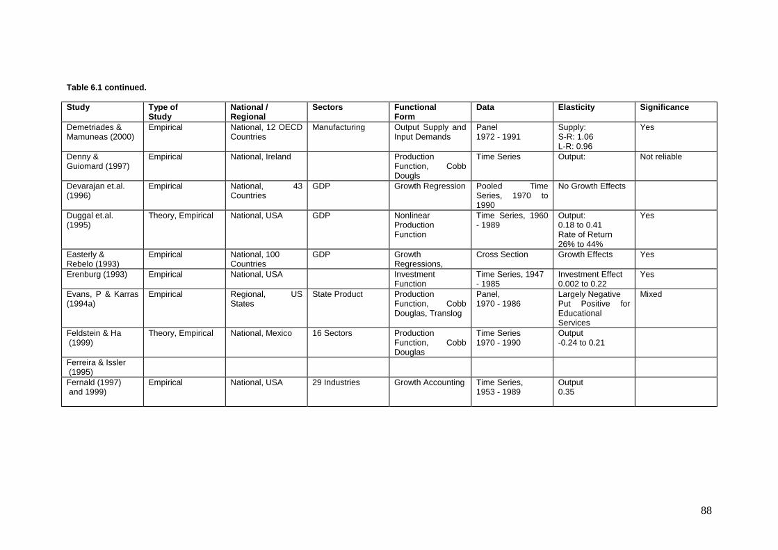
88
Table 6.1 continued. Study Type of
Study National / Regional
Sectors Functional Form
Data Elasticity Significance
Demetriades & Mamuneas (2000)
Empirical National, 12 OECD Countries
Manufacturing Output Supply and Input Demands
Panel 1972 - 1991
Supply: S-R: 1.06 L-R: 0.96
Yes
Denny & Guiomard (1997)
Empirical National, Ireland Production Function, Cobb Dougls
Time Series Output: Not reliable
Devarajan et.al. (1996)
Empirical National, 43 Countries
GDP Growth Regression Pooled Time Series, 1970 to 1990
No Growth Effects
Duggal et.al. (1995)
Theory, Empirical National, USA GDP Nonlinear Production Function
Time Series, 1960 - 1989
Output: 0.18 to 0.41 Rate of Return 26% to 44%
Yes
Easterly & Rebelo (1993)
Empirical National, 100 Countries
GDP Growth Regressions,
Cross Section Growth Effects Yes
Erenburg (1993) Empirical National, USA Investment Function
Time Series, 1947 - 1985
Investment Effect 0.002 to 0.22
Yes
Evans, P & Karras (1994a)
Empirical Regional, US States
State Product Production Function, Cobb Douglas, Translog
Panel, 1970 - 1986
Largely Negative Put Positive for Educational Services
Mixed
Feldstein & Ha (1999)
Theory, Empirical National, Mexico 16 Sectors Production Function, Cobb Douglas
Time Series 1970 - 1990
Output -0.24 to 0.21
Ferreira & Issler (1995)
Fernald (1997) and 1999)
Empirical National, USA 29 Industries Growth Accounting Time Series, 1953 - 1989
Output 0.35

89
Table 6.1 continued. Study Type of
Study National / Regional
Sectors Functional Form
Data Elasticity Significance
Flores de Frutos et.al. (1998)
Empirical National, Spain GDP Production Function, Cobb Douglas Dynamic Analysis
Time Series 1964 - 1992
Output: 0.21
Yes
Ford, R., and Poret, P., (1991)
Empirical National, 11 OECD Countries
GDP TFP , Cross Country Regression
Time Series, 1957 - 1989
MP of Infrastructure 0.45 to 1.7
Yes
Garcia-Mila & McGuire (1992)
Empirical Regional, US States
Gross State Product
Production Function, Cobb Douglas
Panel, 1969 - 1983
Output 0.04
Yes
Garcia-Mila et.al. (1996)
Empirical Regional, US States
Regional Product Production Function: Cobb Douglas
Time Series, Panel
Output: -0.002 to -0.58
No
Grossman (1988) Empirical National, USA GNP Production Function, Cobb Douglas and Non Linear
Time Series, 1929 - 1982
Output 0.03 to 408
Yes
Holtz-Eakin (1994) Empirical Regional, US States
Gross State Product
Production Function, Cobb Douglas
Panel, 1969 - 1986
Output: -0.15 to 0.203
Mixed
Holtz-Eakin & Lovely (1995 & 1996)
Theory, Empirical Regional, US States
Manufacturing Panel Indirect effect
Holtz-Eakin & Schwartz (1995)
Empirical Regional, US States
Gross State Product
Production Function, Cobb Douglas
Panel, 1969 - 1986
Output: 0.03 to 0.05
Yes
Hulten (1996) Empirical National, 42 Countries
GDP Growth Regressions
Cross Section Growth -0.063 to 0.248
Mixed

90
Table 6.1 continued. Study Type of
Study National / Regional
Sectors Functional Form
Time-Series / Cross-Section / Panel
Elasticity Significance
Hulten & Schwab (1991)
Empirical Regional, US States
State Value Added
MFP Time Series, 1951 to 1986
0
Ingram & Liu, Z., (1997)
Empirical National, Regional 50 Countries, 35 Urban Areas
Kavanagh (1997) Empirical National, Ireland GDP Production Function, Cobb Douglas
Time Series, 1958 - 1990
Output No
Keeler & Ying (1988)
Empirical Regional, 9 US Regions
Road Freight Sector
Cost Function, Translog
Time Series, Panel
Cost -0.07
Khan & Kumar (1997)
Empirical National, 95 Countries
GDP Growth Regression
Pooled Time Series, 1970 - 1990
Growth effect 0.13 to 0.29
Yes (large regional differences)
Kocherlakota & Yi (1996)
Empirical National, USA GNP Time Series Analysis
Time Series, 1917 - 1988
Output 0
Yes
Looney & Frederiksen (1981)
Empirical Regional, Mexico Regional Income 'Production Function' Cobb Douglas
Cross Section, Grouped, 1970
Yes

91
Table 6.1 continued. Study Type of
Study National / Regional
Sectors Functional Form
Time-Series / Cross-Section / Panel
Output Elasticity Significance
Lynde (1992) Empirical National US Profit, Cobb Douglas
Time Series MPg: 0.09- 0.27 Profit: 1.2
Yes
Lynde & Richmond (1992)
Empirical National, US Aggregate productive Sector
Share equations, Translog
Time Series, 1958 - 1989
Factor Demand: K 0.71 & 0.90 L -.49 & -0.45
Lynde & Richmond (1993a)
Empirical National, UK Manufacturing Share equations, Translog
Time Series, 1966-1990
Factor Demand K L
Lynde & Richmond (1993b)
Empirical National, USA Profit Function, Share Equations Translog
Time Series, 1958 - 1989
Labour Productivity Growth 0.06
Yes
Lynde & Richmond (1999)
Empirical National, UK Manufacturing DEA Analysis Time Series 1966 - 1990
Mamatzikis (1998) Empirical National, Greece Manufacturing Cobb Douglas Time Series, 1959 - 1993
Output 0.27
Yes
Mas et.al. (1996) Empirical Regional, Spain Regional Output Production Function, Cobb Douglas
Panel 1964 - 1991
Output 0.07 to 0.13
Yes
Merriman (1990) Empirical Regional, Japan, US
Regional Output, by sector
Translog Panel, 1954 -1963
0.43 to 0.58 Yes

92
Table 6.1 continued. Study Type of
Study National / Regional
Sectors Functional Form
Data Elasticity Significance
Morrison & Schwartz (1992 & 1996)
Empirical Regional, US States
Manufacturing Cost Function, Input demand, Generalise Leontief
Time Series, SUR, 1970 -1987
Cost: -0.16 to -0.18 (short run) Productivity growth effects Direct : 0.192 to 0.622 Indirect: -0.027 to 1.442
Yes
Morrison & Schwartz (1996)
Empirical Regional, US States
Manufacturing Cost Function, Input demand, Generalised Leontief
Time Series, 1971 - 1987
Cost: 0.253 (short run) 1.245 (long run)
Munnell ed. (1990) Review, Empirical National, Regional, USA
Production Functions
Time Series Output: 0.055 to 0.11
Yes
Nadiri, I & Mamuneas (1994)
Empirical National, USA Manufacturing Industries
Cost Function, Factor share equations, Translog
Time Series- Cross Section Pooled, 1956 - 1986
Cost -0.1182 to -0.173
Yes
Nagaraj et.al. (1998)
Empirical Regional, Indian States
Growth Regressions
Cross Section Growth -0.37 to 0.46
Otto & Voss (1994) Empirical National, Australia Private sector output, Sectors
Output, Cobb Douglas
Time Series, 1966 - 1990
Output 0.38 to 0.43
Yes
Otto & Voss (1996) Empirical National, Australia Private Sector Output
Output, Cobb Douglas
Time Series 1959 - 1992
Output 0.1675 to 0.2961
Yes
Otto & Voss (1998) Empirical National, Australia Private Sector Output
Cobb Douglas, CES
Time Series 1959 - 1992
Output 0.06 - 0.07
Yes

93
Table 6.1 continued. Study Type of
Study National / Regional
Sectors Functional Form
Time-Series / Cross-Section / Panel
Elasticity Significant
Ram (1986) Empirical Cross Country 'Cobb Douglas' Cross Section Time Series, 1960 - 1980
Marginal Externality -1.41 to 0.5
Find spillovers
Ram & Ramsey (1989)
Empirical National, USA Private Output Cobb Douglas Time Series, 1948 - 1985
Output 0.24
Yes
Ratner (1983) Empirical National, USA Production Function, Cobb Douglas
Time Series 1949 - 1973
Output 0.06
Yes
Rietveld & Boonstra (1995)
Empirical Supply
Rovolis & Spence (1999)
Empirical National, Regional, Greece
Manufacturing & Non- Manufacturing Sectors
Cobb Douglas Time Series, Panel 1982 - 1991
Output Non Man. Sectors: -0.15 to 0.36 Man. Sectors: 0.65 to 0.89 Regions: 0.04 to 0.38
Yes (lots of results)
Seitz (1993) Empirical National, Germany 31 Manufacturing Industries
Cost Function, Input Demand Functions, Generalise Leontief
Panel, 1970 - 1989
Cost: -0.0003
Yes
Seitz (1994) Empirical National, Germany 31 Manufacturing Industries
Cost Function, Factor Demands, Generalised Leontief
Panel, 19770 -1989
Shadow Price: 0.003 to 0.004 Factor Demand: L -0.01 to -0.29 K 0.7 to 0.82
Yes

94
Table 6.1 continued. Study Type of
Study National / Regional
Sectors Functional Form
Data Elasticity Significance
Seitz & Licht (1995)
Empirical Regions, German States
Cost Function, Translog
Panel 1971 -1988
Cost: -0.1 to -0.35
Yes
Shah (1992) Empirical National, Mexico 3 Digit Industries
Cost Function, Input Demand, Translog
Time Series, Pooled, 1970 - 1987
Rate of Return 0.05 to 0.07
Yes
Sturm et.al (1996)
Review, Empirical National, Netherlands
Production Function, Cobb Douglas
Time Series, 1953-1991
0.51 - 1.13 Yes
Vijverberg et.al (1997)
Empirical National, USA Non Financial Corporate Sector
Production, Cost and Profit Function, Cobb Douglas, Semi- Translog
Time Series, 1958 - 1989
inconclusive
Wylie (1996) Empirical National, Canada Manufacturing Production Function Cobb Douglas, Translog
Time Series 1946 - 1991
0.248 - 0.407 Yes

95
6.3 Human Capital The debate on the effect of human capital on aggregate output and growth is still ongoing and no clear consensus has emerged yet. This is despite the fact that at the individual level the returns to schooling have been found to be positive and statistically significant (see Harmon and Walker, 1995 or Barrett, Callan and Nolan, 1999).
One of the main issues is the definition of the human capital variable used in estimation. Thus, some authors use the enrolment rate, i.e. the percentage of the working population of school age which is in (secondary) education at a point in time (Mankiw, Romer and Weil, 1992). However, this does not measure the stock of human capital in an economy at that point in time, but rather measures the future additions to that stock. An alternative measure is the average years of schooling of the labour force which is a measure of the stock of human capital (Benhabib and Spiegel, 1994). However, even this measure is far from perfect since it does not account for school quality which some researchers measure using the amount spent on education. Of course higher expenditure does not automatically result in better quality of education, particularly if a substantial proportion of the funds are used in an inefficient way. It is beyond the scope of this paper to settle this debate and we therefore simply review some of the interesting results which have been obtained.
In an influential paper, Mankiw, Romer and Weil (1992) found using a cross country data set that the output elasticity with respect to human capital, as measured by the secondary school enrolment rates, is in the region of 0.3. This work has been extended by Nonneman and Vanhoudt (1996), who find that elasticity to be somewhat smaller at 0.15. Further corroborating evidence for this result has been put forward by Demetriades, Arestis and Kelly (1998), who, using mean years of schooling as a proxy for human capital, find the output elasticity to be 0.37.
Griliches and Regev (1995) use a labour quality index which is based on the mix of academic qualifications in the labour force in a study of firm productivity in Israeli industry. These authors find the elasticity of output per worker with respect to labour quality to fall in the range between 0.14 and 0.74.
The above papers all use the level of the human capital proxy in regressions with the level of output as the dependent variable. This suggests that growth rates should be related positively to rate of change of these human capital proxy measures. However there is evidence which suggests that this is not so. Benhabib and Spiegel (1994), again in a cross country setting, find that the change in educational attainment affects growth negatively though not statistically significantly. Furthermore they find weak evidence for a positive impact of the level of human capital on the growth rate of output. Finally they find that the level of human capital has a positive and often significant effect on investment, which suggests that human capital affects the rate of technological innovation as well as the speed of the adoption of new technologies.
Further evidence supporting the link between the level of human capital and output growth is provided by Barro (1991), using enrolment rates, and by Barro and Sala-I-Martin (1995), using secondary and higher level educational attainment. However the latter only find male secondary and higher level educational attainment has a statistically to have a significant positive impact on growth, while the same variables for females has a negative, though not statistically significant, effect on growth.57
This brief review indicates that, on balance, human capital is likely to have a positive impact and that the output elasticity is in the range of 0.15 to 0.4. However, there appears to be scope for further work in this area. In particular, the existing literature has yet to address the 57 In should be noted that recent work by Rodrik (2005) casts considerable doubt on the utility of growth regressions in the investigation of the policy impacts of public investment programmes.

96
issue of spillovers of human capital as there has been no attempt to estimate the productivity effect of the presence of a highly educated worker on a worker who with lower human capital.
6.4: Measuring human capital If one is to study the relationship between human capital and growth, it is necessary to have a methodology for measuring the level or the flow of human capital. In most studies in this area a simple approach is adopted that does not distinguish between the level at which the education takes place (see Sianesi and Van Reenen, 2002 for a comprehensive survey). In such approaches, years spent in education are simply counted and years in primary school are treated in the same way as years spent in university. This simplification is often necessitated by the unavailability of data for many countries. However, in the case of many of the countries covered in the HERMIN models of the COHESION System, reliable and comparable data are collected annually by the OECD, together with a common classification of different types of education.
In order to measure the impact of that proportion of the EU cohesion policy funding that were, or are to be, devoted to the development of human capital, the starting stock of human capital is needed. If the cohesion policy evaluation is an ex-post one, focused on the period 2000 to 2006, then this starting stock is needed for the year 1999 (i.e., the year prior to the implementation start-up). If the evaluation is an ex-ante one, focused on the period 2007 to 2013, then this starting stock is needed for the year 2006.
The most basic variable that is required to measure the stock of human capital is the educational attainment of the population. This simply records the percentage of the population by their highest level of attainment. The breakdown chosen by the OECD refers to four levels of educational attainment:
i. Primary and lower secondary education (PS) ii. Higher secondary education (HS) iii. Non-university tertiary education (NUT) iv. University education (UT)
Primary and lower secondary education are grouped together since these are the most basic levels of education and lower second level education tends to be the minimum level of education at which children leave school. Table 6.2 shows that there were large differences between many of the EU states by the middle of the last decade. For example, Portugal has a very high percentage of the population in the primary and lower secondary group and consequently only small percentages in the higher groups. The opposite is true for Germany.
Table 6.2: Educational Attainment:
Percentage of population classified by highest level of attainment (1994)
Primary and Lower Secondary
Higher Secondary
Non University Tertiary
University Tertiary
Greece 55 27 6 12 Ireland 55 27 10 9
Portugal 81 8 3 7 Spain 74 11 4 11
Germany 16 62 10 13 Italy 67 26 8 UK 26 54 9 12
Source: OECD Education at a Glance, 1996

97
Table 6.2 refers to the whole population and ignores generational differences. In order to further evaluate these differences, it is useful to analyse the educational attainment of persons aged 25 to 34 years. This also yields a more accurate picture of the likely future development of human capital. Table 6.3 shows particularly low rates of attainment in Portugal, Spain and Italy.
Table 6.3: Educational attainment:
Percentage of the population aged 25 to 34 which has attained at least upper secondary or third level education, 1995
Upper Secondary and
Higher Tertiary
education Greece 64 26 Ireland 64 27 Portugal 31 14 Spain 47 27 Germany 89 21 Italy 49 8 UK 86 23
Source: OECD Education at a Glance, 1997 The usual measure of human capital in the economic literature is years of schooling. However, this variable ignores the important differences between the educational systems of the countries in question, and this can introduce biases into the measure of human capital. Table 6.4 highlights these difference by giving details of the typical cumulative years of schooling required to complete a particular level. For example, in order to complete lower secondary level education, a pupil in Ireland, Spain and Germany will spend 10 years in school, while students in Portugal and Italy require just 8 years. The table also shows the additional years that are required to attain the next highest level of education which can be readily worked out by subtracting the years required for the lower level from the years required for the higher level. It should be noted that the University level does not build on the non-university tertiary level. Rather, both tertiary levels tend to be achieved at the same time by different non-overlapping groups, and build on the higher secondary levels.
Table 6.4: Cumulative years of schooling required to attain
a specified level of education (1994)
Primary and Lower Secondary
Higher Secondary
Non University Tertiary
University Tertiary
Greece 9 12 15 23 Ireland 10 13 15 16 Portugal 8 12 14 16 Spain 10 12 14 17 Germany 10 13 15 19 Italy 8 13 13 20 UK 9 13 15 16
Source: OECD Education at a Glance, 1996 A further issue that arises is the fact that the participation in the labour force is not equal for all levels of educational attainment. As is indicated from Table 6.5 below, persons with a lower level of education are less likely to participate in the labour force than those with a

98
higher level of education. This clearly reflects the fact that those with a higher level of education have invested more in their education and are therefore seeking a return to their investment as well as the fact that these individuals also tend to have more opportunities to gain employment since their skill are more in demand. Of course this also means that a given programme that increases the human capital of individuals will not result in all individuals finding employment or even seeking employment.
Table 6.5: Labour force participation by educational attainment (percentage, 1994)
Primary and Lower Secondary
Higher Secondary
Non University Tertiary
University Tertiary
Total
Greece 62 67 84 87 67 Ireland 58 73 85 89 67 Portugal 72 84 87 95 75 Spain 58 80 88 87 65 Germany 56 76 85 88 75 Italy 58 73 85 89 67 UK 64 82 87 91 79
Source: OECD Education at a Glance, 1996 These patterns of behaviour influenced the manner in which the measure of stock of human capital was specified in the HERMIN country models, as explained in Chapter 4, Section 4.4, above.
6.5 The role of R&D The quantification of the likely impacts of investment spending on R&D is the most difficult to analyse. Most research in the area consists of theoretical explorations of the role of R&D in promoting growth, within the context of new theory-based models of endogenous growth. Empirical research into R&D impacts remains at an early and experimental stage. An extensive survey of research has been carried out by the US Congressional Budget Office (CBO, 2005). Unfortunately, most of the empirical investigation centres of the analysis of cross-sectional data at a specific point in time. This is to be contrasted with the analysis of time series data over an extended period of time. The CBO survey suggests that the impacts of R&D derived from cross-sectional studies tend to be both larger and more significant than those derived from time series analysis. The CBO survey also suggests that the returns from public investment in R&D tend to be lower than the returns from R&D carried out by the private sector. Finally, the empirical findings are even less robust than those found in comparable analysis of the impacts of physical infrastructure and human capital on output. One possible implication for the HERMIN model is that one might consider setting the spillovers (or externalities) of R&D investments of cohesion policy at zero. In that case, there would only be transitory Keynesian impacts during the implementational period, which would vanish after the programme is terminated. We feel that this is an extreme position to adopt. But the alternative of setting the rates of return from R&D investment at the values typically found from physical infrastructure and human capital would also be extreme, and probably unrealistically optimistic. In subsequent analysis we adopt very low values of the spillover (or externality) elasticities of output and productivity with respect to increases in the stock of R&D. A more precise analysis and quantification will have to be postponed until there is greater detail on the exact nature of the cohesion policy R&D measures, and until the international literature progresses.

99
[7] From CP financial tables to CP investment types The planned expenditures on cohesion policy (CP) are usually first available in the form of Financial Tables that set out the data classified into measures and Operational Programmes (OPs). But before these data and their content can be used for the analysis of the impact of cohesion policy, it is necessary to bring them into a form that can be handled inside the COHESION System of economic models. In other words, the data from the Financial Tables must first be mapped into the three types of investment that are incorporated in the model mechanisms: physical infrastructure, human resources and direct support of the productive sector. This process is carried out “off-model” in a series of sophisticated spreadsheet files that take in the published data from the Financial Tables, and generate the required transformation of these data into the investment types. It is made up of the following stages: Stage 1: DG Regional Policy, in association with the member states, is responsible for the production of the Financial Tables. Although these may vary in format, we assume that they are in the form of a spreadsheet file for all countries called “FIELD OF INTERVENTION.XLS”. This file must contain a description of the measures used in a specific country. The following screenshot shows an extract from this spreadsheet, taken from an ex-ante study of the impacts of the CP 2007-2013 programme:
Stage 2: The COHESION System of models requires that the Financial Tables be reclassified by economic types of investment goods. Three economic categories of investment are used within the HERMIN models of the COHESION System, and are defined as follows:

100
i. Physical infrastructure (henceforth, PI) ii. Human resources (henceforth, HR) iii. Aid to the productive sectors (henceforth, APS)
In the case of APS, we distinguish between aid to manufacturing, market services and agriculture. Furthermore a R&D sub-category of total APS is introduced, since a specific share of the aid to the productive sectors is designated for investment in R&D activities. A country specific spreadsheet file is set-up to perform all the needed calculations, and is explained below. Stage 3: Taking Estonia (EE) as an example, the spreadsheet NSRF_HEE5_ESTONIA.XLS contains the following five work sheets
Economic categories: This is the worksheet where all the categorisation of the measures is performed. As an additional measure the national co-finance rate is calculated.
SF for Estonia: This is the worksheet where decisions are made concerning allocations from OPs to investment categories, and calculations are performed (all blue highlighted cells may be changed by the user) (a) Different scenarios can be defined (e.g., A,B,C). The examples here are taken from the Spring 2007 ex-ante study carried out for DG Regional Policy, using the first operational version of the COHESION System.

101
(b) Indexation, defining an inflation rate (since the initial EC cohesion funding may be defined in constant (initial) year prices.
(c) Setting the co-financing rate (national and private), as required by EC regulations.
(d) The Lisbonisation “rules”: These are designed to explore stylised variations of the so-called Lisbon Strategy, where there is a greater emphasis on investment in HR and R&D (i.e., a subset of APS), and less emphasis on PI.
(e) Distribution into economic categories. This is carried out in the work sheet Economic categories. The allocation of the cohesion policy financial data into PI, HR and APS (including R&D) is not a completely standardised process, but has an element of judgement. The more detailed is the information available in the Financial Tables, the more accurate can be the re-classification into investment categories.
(f) Finally, the SF financial data for the period 2000 – 2006 and 2007 – 2013 are inserted from the spreadsheet provided by DG Regional Policy.

102
Stage 4: After the above decisions have been made, provision is made for up to three further worksheets to be defined, in the case where we can assume three different cohesion policy scenarios (referred to as A, B and C below):
i. NSRF EC data inputs (A) ii. NSRF EC data inputs (B) iii. NSRF EC data inputs (C)
These are generated and recalculated automatically from the previous worksheet, whenever any changes are made to the basic decisions, and can then be used as direct input to the relevant parts in the WINSOLVE model simulation files that perform the analysis of cohesion policy impacts. These WINSOLVE simulation files are “batch” files that execute the analysis in a standard way. Examples will be given later, and in the Annexes, based on the Spring 2007 ex-ante analysis of the 2007-2013 programme. For example, the worksheet NSRF EC data inputs (B) for Estonia is as follows:
The data from this worksheet can simply be read off and directly pasted into the WINSOLVE simulation file. Examples will be provided later.

103
[8] Testing the COHESION country models
8.1 Introduction In Chapter 5 we described the first stage of model testing, namely the calibration of the model. We now move to further testing, starting with the simulations that were designed to check the within-sample tracking performance. It should be stressed that HERMIN is not a model designed for short-term forecasting. It includes none of the special fixes and dummy variables that are commonly used to ensure good within-sample performance in many short-term forecasting models. But it needs to be stressed that good within-sample tracking is usually achieved at the expense of dispensing with a sound theoretical structure and coherent medium-term performance. In this section we describe how the individual country models can be subjected to a battery of further tests with the object of examining the performance of the system of equations as a whole. We first describe briefly the process of checking the model structure by forcing the model’s behavioural equations to track the within-sample data exactly (i.e., “fixing” of intercept adjustments or “add-factors” for the behavioural equations of the model). Then we describe how the model is subjected to a series of standard exogenous and policy shocks in order to explore the pattern of its responses.
8.2 Checking the model structure Even though the model is primarily designed for policy oriented experiments of a complex kind, we do not completely neglect its within sample tracking performance. Not only is a reasonable within sample tracking a necessary condition for the model to be realistic, but it would also point out the weak parts of the model, i.e. the behavioural equations whose calibration neglected some important factors, or identities that were mis-specified. Therefore checking of the model’s within sample properties provides valuable information on the quality of the calibration process and is used in the design stage of model construction, when modellers often have to return back to the calibration stage if such checks produce unsatisfactory results. The control of the within sample performance is initially carried out by a means of a so-called “residual check” simulation. Once the individual behavioural equations have been calibrated, and the model as a parameterised system of equations is set up, we run a static simulation which uses the historical values of the endogenous and exogenous variables on the right hand side of every equation of the model to compute the endogenous (behavioural or identity) variable that is designated as being determined by this equation. The resulting values of the endogenous variables for every simulated year of the sample is then compared to their actual historical values. More specifically, we are interested in the percentage difference of the simulated from actual values. There is no obvious benchmark as to what percentage difference constitutes a reasonable fit of an equation. Rather, it varies from a case to case, but overall we aim at less than 10 per cent difference for all of the more important behavioural variables. Of course, variables computed as identities must, by definition, fit exactly if simulated in this “single-equation” way, up to a numerical rounding error. In addition, we also want these differences for each behavioural variable to change signs over time, suggesting a random error. If this residual check produces unsatisfactory results, we can revert back to calibration of the most

104
troublesome equations and carry out a review the equation specification. In the case\of the present models in the COHESION System, we finished with most behavioural variables showing less than 5 per cent difference from the historical values in every year. The main exceptions were investment variables, which are very difficult to track with a model of the highly constrained type that we specify.58 On balance, the within sample tracking results boosted our confidence in the ability of the model to reflect reality reasonably well. However, it falls far short of the rigorous testing normally carried out on econometric models, where long and stable time series of data are available and support rigorous econometric analysis. It should also be recalled that most of the country HERMIN models in the COHESION System have only recently emerged from a transition from central planning to market-based institutions, and have little previous experience of econometric research and modelling due, mainly, to the short time span of data that are available. In many cases, the HERMIN country models are the first examples of such econometric models to be constructed. Having performed the residual check procedure described above, we can then carry out the usual kind of within-sample static and dynamic system simulations. In static system simulations, the model is re-started every time period, and the historical data used for lags. In dynamic simulations, on the other hand, the model is started at some point in time, and the solution values are used for lags in subsequent periods. The dynamic simulation is a more searching test of model performance than the static simulation. We obviously want to use the information on the magnitude of error that the individual equations display during the within sample check, in the out of the sample projections and simulations. In order to do so, we carry out a static, within sample simulation as before, but this time we solve each equation independently and not as part of the simultaneous system (i.e., a “residual checking” simulation). We then compute absolute differences between the simulated and true values. These absolute differences are used to create the so called constant adjustment (or CA) factors each year for each behavioural variable. These adjustment factors act, effectively, as corrections to our estimates of behavioural intercepts in each behavioural equation, with the property that they make the computed “behavioural” variable exactly fit the within sample data. Therefore, if we add these constant adjustment factors back to each behavioural equation we will obtain a perfect fit of the whole model, within sample. What is more important, though, is that we can use this information on the error in our behavioural intercepts in the out of the sample projections and simulations, as will be described in the next chapter, when we describe how baseline projections can be prepared.
8.3 Shocking the model59
We can examine the properties of any HERMIN model using a series of simulated shocks to exogenous variables. In order to examine the full medium-term properties of the model, we need to simulate the model over a long period. To do this, we use a baseline projection for the period 2006 to 2020, since the year 2006 is the last one for which historical data are
58 The highly constrained specification of the factor demand systems in manufacturing, building and market
services is an essential requirement if the model is to be useful in the analysis of the long-term impacts of cohesion policies. Refer to Chapter 3, section 5 for full details of the CES production function and factor demand specifications.
59 In Section 8.3 we continue to present the results of shocks as derived using the September, 2007 version of the COHESION System. Updated versions of these tests can be easily derived using the series of WINSOLVE batch files supplied with the computer installation.
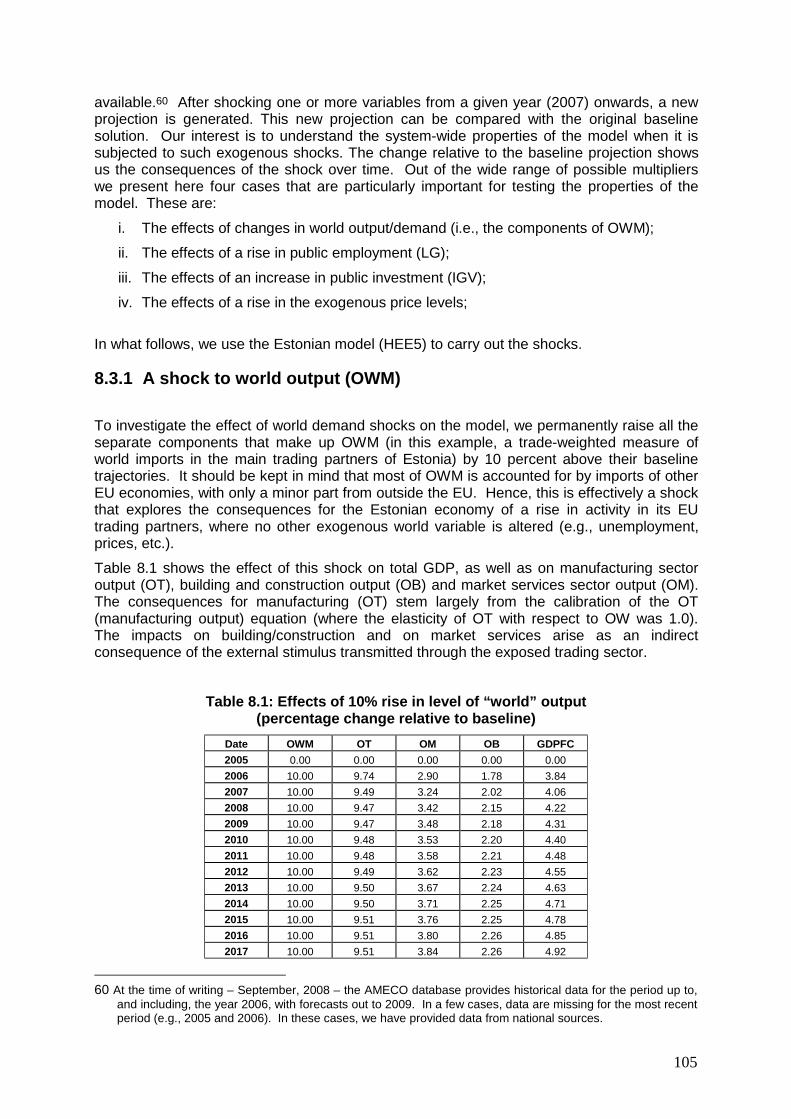
105
available.60 After shocking one or more variables from a given year (2007) onwards, a new projection is generated. This new projection can be compared with the original baseline solution. Our interest is to understand the system-wide properties of the model when it is subjected to such exogenous shocks. The change relative to the baseline projection shows us the consequences of the shock over time. Out of the wide range of possible multipliers we present here four cases that are particularly important for testing the properties of the model. These are:
i. The effects of changes in world output/demand (i.e., the components of OWM);
ii. The effects of a rise in public employment (LG);
iii. The effects of an increase in public investment (IGV);
iv. The effects of a rise in the exogenous price levels;
In what follows, we use the Estonian model (HEE5) to carry out the shocks.
8.3.1 A shock to world output (OWM)
To investigate the effect of world demand shocks on the model, we permanently raise all the separate components that make up OWM (in this example, a trade-weighted measure of world imports in the main trading partners of Estonia) by 10 percent above their baseline trajectories. It should be kept in mind that most of OWM is accounted for by imports of other EU economies, with only a minor part from outside the EU. Hence, this is effectively a shock that explores the consequences for the Estonian economy of a rise in activity in its EU trading partners, where no other exogenous world variable is altered (e.g., unemployment, prices, etc.).
Table 8.1 shows the effect of this shock on total GDP, as well as on manufacturing sector output (OT), building and construction output (OB) and market services sector output (OM). The consequences for manufacturing (OT) stem largely from the calibration of the OT (manufacturing output) equation (where the elasticity of OT with respect to OW was 1.0). The impacts on building/construction and on market services arise as an indirect consequence of the external stimulus transmitted through the exposed trading sector.
Table 8.1: Effects of 10% rise in level of “world” output (percentage change relative to baseline)
Date OWM OT OM OB GDPFC 2005 0.00 0.00 0.00 0.00 0.00 2006 10.00 9.74 2.90 1.78 3.84 2007 10.00 9.49 3.24 2.02 4.06 2008 10.00 9.47 3.42 2.15 4.22 2009 10.00 9.47 3.48 2.18 4.31 2010 10.00 9.48 3.53 2.20 4.40 2011 10.00 9.48 3.58 2.21 4.48 2012 10.00 9.49 3.62 2.23 4.55 2013 10.00 9.50 3.67 2.24 4.63 2014 10.00 9.50 3.71 2.25 4.71 2015 10.00 9.51 3.76 2.25 4.78 2016 10.00 9.51 3.80 2.26 4.85 2017 10.00 9.51 3.84 2.26 4.92
60 At the time of writing – September, 2008 – the AMECO database provides historical data for the period up to,
and including, the year 2006, with forecasts out to 2009. In a few cases, data are missing for the most recent period (e.g., 2005 and 2006). In these cases, we have provided data from national sources.
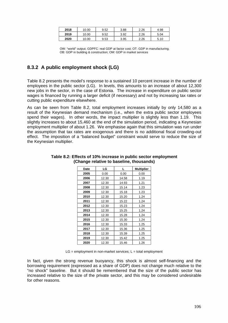
106
2018 10.00 9.52 3.88 2.26 4.98 2019 10.00 9.52 3.92 2.26 5.04 2020 10.00 9.53 3.95 2.26 5.10
OW: “world” output; GDPFC: real GDP at factor cost; OT: GDP in manufacturing; OB: GDP in building & construction; OM: GDP in market services
8.3.2 A public employment shock (LG)
Table 8.2 presents the model’s response to a sustained 10 percent increase in the number of employees in the public sector (LG). In levels, this amounts to an increase of about 12,300 new jobs in the sector, in the case of Estonia. The increase in expenditure on public sector wages is financed by running a larger deficit (if necessary) and not by increasing tax rates or cutting public expenditure elsewhere.
As can be seen from Table 8.2, total employment increases initially by only 14,580 as a result of the Keynesian demand mechanism (i.e., when the extra public sector employees spend their wages). In other words, the impact multiplier is slightly less than 1.19. This slightly increases to about 15,460 at the end of the simulation period, indicating a Keynesian employment multiplier of about 1.26. We emphasise again that this simulation was run under the assumption that tax rates are exogenous and there is no additional fiscal crowding-out effect. The imposition of a “balanced budget” constraint would serve to reduce the size of the Keynesian multiplier.
Table 8.2: Effects of 10% increase in public sector employment (Change relative to baseline, thousands)
Date LG L Multiplier 2005 0.00 0.00 0.00 2006 12.30 14.58 1.19 2007 12.30 14.93 1.21 2008 12.30 15.14 1.23 2009 12.30 15.18 1.23 2010 12.30 15.20 1.24 2011 12.30 15.22 1.24 2012 12.30 15.23 1.24 2013 12.30 15.25 1.24 2014 12.30 15.28 1.24 2015 12.30 15.30 1.24 2016 12.30 15.33 1.25 2017 12.30 15.36 1.25 2018 12.30 15.39 1.25 2019 12.30 15.42 1.25 2020 12.30 15.46 1.26
LG = employment in non-market services; L = total employment
In fact, given the strong revenue buoyancy, this shock is almost self-financing and the borrowing requirement (expressed as a share of GDP) does not change much relative to the “no shock” baseline. But it should be remembered that the size of the public sector has increased relative to the size of the private sector, and this may be considered undesirable for other reasons.

107
8.3.3 A shock to government investment (IGV)
The next shock we describe relates to an increase in public investment in infrastructure. Table 8.3 shows the effect of a permanent 10 percent increase in nominal public investment. As can be seen from Table 8.3, there is a initially modest Keynesian multiplier effect of less than unity (i.e., the change in real GDP (GDPE) divided by the shock to real public investment (IG)). The multiplier on GDP rises to 1.05 by the year 2010, and to 1.15 by the year 2020.
Once again, we must stress that the extra public expenditure to support increased public investment is financed by running a higher public sector deficit. So, there is no fiscal crowding out due to higher tax rates or higher interest rates (since interest rates are exogenous). It should also be stressed that in shocking public investment, IGV, we only look at the expenditure impacts, and make no assumptions concerning any supply-side benefits that may arise from these investments. As we saw above, in the case of cohesion policy shocks one obtains both a Keynesian effect as well as a supply-side impact, due to the beneficial effects of increases in the stocks of physical infrastructure, human resources and R&D.
Table 8.3: Effects of a 10% rise in the level of public investment (change relative to baseline, real EEK (2000))
Date IG I CONS NTS GDPE Multiplier 2005 0.00 0.00 0.00 0.00 0.00 0.00 2006 473.27 591.56 249.09 -402.62 437.92 0.93 2007 471.35 601.53 283.38 -419.79 464.85 0.99 2008 470.69 605.57 298.88 -423.97 480.13 1.02 2009 470.44 604.48 304.13 -421.79 486.37 1.03 2010 470.26 603.10 308.11 -419.02 491.62 1.05 2011 470.09 601.64 311.86 -416.17 496.61 1.06 2012 469.93 600.18 315.61 -413.36 501.51 1.07 2013 469.77 598.73 319.38 -410.62 506.34 1.08 2014 469.61 597.28 323.18 -407.93 511.10 1.09 2015 469.45 595.85 327.00 -405.29 515.78 1.10 2016 469.29 594.42 330.86 -402.67 520.37 1.11 2017 469.13 592.99 334.73 -400.07 524.87 1.12 2018 468.96 591.56 338.61 -397.46 529.26 1.13 2019 468.78 590.12 342.51 -394.81 533.53 1.14 2020 468.59 588.67 346.42 -392.08 537.68 1.15
IG = real public investment; I = total investment; GDPE = GDP (expenditure); NTS = real net trade surplus; CONS = private consumption
8.3.4 A shock to all exogenous price levels
Here we carry out a shock that raises the exogenous price levels permanently by 10 percent, mainly in order to test the price homogeneity that was imposed on the model. The prices involved are as follows: the price of agricultural output (POA); the price of manufacturing output in the world (with various subcomponents); and the import price (PM).
Table 8.4 illustrates the response of prices and costs in the case of Estonia. The delay in adjustment is due entirely to the phased adjustment of prices in market services and building.

108
Table 8.4: Effects of 10% increase in all exogenous price levels (percentage change relative to baseline)
Date PWORLD POT POM PCONS WT ULCT RULCT 2005 0.00 0.00 0.00 0.00 0.00 0.00 0.00 2006 10.00 9.12 6.57 8.17 7.97 7.98 -1.05 2007 10.00 9.28 8.42 8.99 8.79 8.79 -0.45 2008 10.00 9.32 8.66 9.10 8.96 8.96 -0.33 2009 10.00 9.34 8.72 9.14 9.01 9.01 -0.30 2010 10.00 9.35 8.75 9.15 9.04 9.04 -0.28 2011 10.00 9.36 8.78 9.17 9.06 9.06 -0.27 2012 10.00 9.37 8.80 9.18 9.08 9.08 -0.26 2013 10.00 9.38 8.83 9.20 9.10 9.10 -0.25 2014 10.00 9.39 8.85 9.21 9.12 9.12 -0.24 2015 10.00 9.40 8.88 9.22 9.14 9.14 -0.24 2016 10.00 9.41 8.90 9.24 9.16 9.16 -0.23 2017 10.00 9.42 8.92 9.25 9.18 9.18 -0.22 2018 10.00 9.43 8.95 9.26 9.20 9.20 -0.21 2019 10.00 9.44 8.97 9.28 9.22 9.22 -0.20 2020 10.00 9.45 8.99 9.29 9.23 9.23 -0.20
PWORLD = World price; POT = manufacturing output deflator; POM = market services output deflator; PCONS = Consumption deflator; WT = Average annual earnings in manufacturing; ULCT = unit labour costs, manufacturing; RULCT: Real unit labour costs, manufacturing
8.3.5 Conclusions on responses to shocks
The shocks illustrate some of the properties of the five-sector versions of the HERMIN models that make up the COHESION System. For example, world market conditions feed into the economy of Estonia mainly through the internationally exposed manufacturing sector but also indirectly through the market services sector. Much the same behaviour is displayed by the other models in the system. External price shocks pass quickly into domestic prices, under the assumption of a fixed exchange rate. Public employment and investment shocks have relatively modest Keynesian impacts on the economy. However, it must be recognised that the public employment (LG) and public investment (IGV) shocks impact mainly on the demand side of the economy. In the next section we show how these demand-side (or Keynesian) impacts can be augmented through supply-side productivity-enhancing effects that are associated with EU Structural Funds.
The above set of tests serve to alert us to the importance of the market services and building and construction sectors (i.e., the mainly non-traded sectors). The latter is destined to play a major role in the implementation of the physical infrastructure investment programmes of the cohesion policies, which will absorb a high proportion of the funding. They also demonstrate the rather different properties of the manufacturing sector, due to its direct exposure to the global economy, its more limited exposure to the domestic economy, and the role played by international competitiveness.

109

110
[9] Issues in constructing baseline projections
9.1 Introduction One of the most common activities carried out by economists working in the public and private sectors involves the preparation of economic forecasts. Most of the published forecasts focus on the immediate future, and have a time horizon of about one year, or perhaps 18 months, at most. Most are also constructed on the basis of special knowledge and the personal judgement of the analysts. The most influential forecasts tend to be those that are prepared by the most prestigious institutions, either internationally (by organisations such as the European Commission in Brussels (DG-ECFIN), the Paris-based OECD, or by the IMF in Washington), or nationally (e.g., by national Ministries of Finance, Central Banks or other NGOs). It is when one attempts to carry forecasts out into the medium term, with time horizons of up to five or more years, that the real difficulties begin. First, very few national organisations prepare forecasts of medium-term prospects. Second, even when such forecasts are prepared, they are seldom published formally, even if they are used internally inside government agencies as background inputs to medium-term policy making. Third, it is often the case that medium-term forecasts are prepared by simply running the short-term methodologies out into the medium term, even when such methodologies may be completely inappropriate. Before we turn to forecasting issues using the HERMIN models of the COHESION System, it is important to emphasise the context within which forecasts are prepared. National governments need to monitor economic performance, and to anticipate future trends, for two reasons. First, they need to understand the consequences of the international forces that shape their economies, but over which they have little or no control. The most obvious examples include the nature and timing of changes in the international business cycle; technological innovations; “shocks” to oil and other commodity prices, etc. Second, they need to be able to design and use economic policies to improve the environment within which businesses function efficiently as well as improve the welfare of households. The task of monitoring and anticipating international trends, as well as designing and evaluating public policy, draws its authority from the existing pool of academic and applied research in economics, both domestic and international. If a country faces major policy challenges, but either has an inadequate stock of research-based knowledge or fails to draw comprehensively from its available pool of research, then policy design and evaluation are less likely to be soundly based or effective. Access to applied economic and business research is a necessary condition for good policy-making, but is certainly not sufficient. From the point of view of policy analysts engaged in the preparation of forecasts, research is most useful when it is “quantitative” in nature. This requires that there be formal studies of the most important mechanisms in the economy, such as the functioning of the labour market, the determination of prices, the nature of the production process, consumer behaviour, etc. In most “old” EU member states, there is usually a long “back catalogue” of research findings to draw from. However, in the new member states of the COHESION System, where a market economy was only slowly created after the 1989 liberalisation, there is less accumulated research from which to draw. A particularly useful vehicle for quantitative economic research is when isolated and unconnected research findings are brought together and consolidated into formal policy

111
models, which attempt to examine all the major mechanisms in the economy within a single system. This is the goal of the COHESION System of models. But it should be emphasised that such macro-economic models are only as good as the underlying quantitative research from which they draw their authority. Economic models have come to play a crucial role in policy analysis and forecasting. This role is more important for the longer term than for the shorter term, but having a systemic or holistic view of the economy is useful even for ad-hoc short-term forecasting exercises. Indeed, it can be said that policy analysts and forecasters always use models, consciously or unconsciously. These models can be “informal” or “formal”. The use of “informal” models tends to be more widespread, particularly for short-term forecasting. There are many reasons for this situation. First, “informal” models can treat the parts of the economy in isolation from each other, and avoid the need for rigorous consistency checking (e.g., are the public finances consistent with assumed developments in private sector activity?). Second, the economy is a complex, changing, often unstable system that can be very difficult to formalise convincingly in mathematical equations. And even if formalised models of the economy could be developed, they would require time, technical skills, and other resources that are often in short supply. Third, even if resources were devoted to model building, the data restrictions in the economies of the NMS are serious, and will usually support only relatively unsophisticated models.61
9.2 Short-term forecasting It may be unwise to consider setting up a serious medium-term forecasting exercise unless one has already in place an adequate short-term forecasting system. If one were to attempt to prepare a medium-term forecast of a typical new member state economy at the time of writing (September, 2008), one would be faced with a situation where the most recent complete official national accounting data were for the year 2006, with the prospect of having data for 2007 in the immediate future. Partial information is available for 2007, but this usually takes the form of short-term forecasts (or perhaps, more accurately, “backcasts”). Setting up a short-term forecasting system essentially involves a database of economic indicators of recent performance, as well as indicators of likely performance in the immediate future. These data can come from a variety of sources:
i. Statistical releases issued by the Central Statistics Office;
ii. Economic commentary in the financial press, prepared by economic research agencies and internally by the media;
iii. Official releases by the monetary authority, as well as by other private banks;
iv. Publications issued by trade organisations and private companies, in the form of
annual reports, etc.;
v. International forecasting publications that focus on the immediate past and the immediate future.
The most common framework for short-term forecasting is the simple Keynesian income-expenditure framework. Typically, one starts with forecasts of exports, and then prepares
61 For example, the NMS HERMIN models are based on 12 annual observations at most, covering the period 1995-2006. This is too small a data sample to use for conventional econometrics.

112
forecasts of the other elements of GDP on the expenditure side of the national accounts: private consumption, public consumption, investment, stock-changes and imports. In each case there is usually a range of indicators to guide the forecast, such as investment intentions, consumer surveys, recent government budgets, etc. Having forecast GDP on the expenditure basis, one then proceeds to the income side of the national accounts. In the case of wage rates, there is usually evidence of recent trends, and indications of likely future changes over a horizon of about one year. The wage rate forecasts are then combined with employment projections (derived from, and linked to the GDP forecast already made), and this yields the wage component of GDP on an income basis. Corporate profits are then derived residually as GDP on the expenditure basis, minus wage income. In short-term forecasts, the public finances are usually handled separately, and official projections often accepted unquestioned. The same applies to the balance of payments on current account (except, of course, for the net trade balance, which is obtained from the expenditure-side forecasts). The derivation of short-term forecasts seldom make use of formal economic models. Rather, a consistency check is operated through the income expenditure identity, usually by means of a computer-based spreadsheet. An initial forecasting round is carried out, and the income expenditure identity checked, with emphasis on items calculated residually. The process then goes through a series of iterations, until a satisfactory and acceptable result is obtained. To the extent that they involve genuine forecasting activities (as distinct from reliance on leading indicators), short-term forecasts are judgemental. The income-expenditure consistency framework can be used to improve the forecasts, but little use is made of formal economic research. For the “ragged edge” period (i.e., the period from the last complete set of officially published national accounting data to the date on which the forecast is made), this approach serves to optimise the use of partial information in order to derive a complete picture of the state of the economy in the present and in the immediate past. But judgemental forecasts are usually unreliable beyond about 12 to 18 months into the future. To move further into the future requires a more formalised methodology based on model systems. To summarise, short-term forecasts usually review the previous 12 months and project the next 12 to 18 months. An “informal” model approach is used:
(a) Leading indicators are used to forecast the likely external economic environment (b) The fiscal stance is taken from the most recent budget (c) The main expenditure components of GDP (exports, private consumption,
investment, stock changes and imports) are forecast, using leading indicators and judgement.
(d) Wages and prices are forecast using leading indicators and judgement (e) Profits are residually determined from the income-expenditure identity (f) Output is determined by the level of demand
The above approach could be said to be based loosely on a “model”, in the sense that the Keynesian income-expenditure framework is used. But the model is “informal” in the sense that relationships are not expressed analytically, are not subject to any testing and stability analysis, and probably represent a small subset of knowledge of how the economy works. Such an approach is useful in the short term, when structures are relatively stable, policy decisions are pre-set, and the demand-side mechanisms (which operate in the short-term) dominate the supply-side mechanisms (which operate in the longer term).

113
9.3 Issues in medium and long-term forecasting We discussed above how “informal” models can be used in the preparation of short-term forecasts. But as one shifts the time horizon outwards, beyond 12 months, informal approaches become less useful. There are many reasons for this, and a longer-term forecasting perspective has many different requirements beyond those used in short-term forecasting. First, in the longer term underlying structures are changing over time. Examples include the capacity and sectoral structure on the economy, and of agriculture, manufacturing and market services in particular. Technology is also changing, as old products decline and new products rise, with serious implications for the productive sectors. Also, the economy’s external orientation may be shifting. In the case of the NMS, they are becoming more open to international trade with other EU member states, and receives a growing share of inward direct investment. Second, in the short term, the international environment is known, at least to some degree. NMS short-term forecasters can draw on a wide range of authoritative forecasts of the international environment and use these to set the international context for the NMS economies. However, over the longer term, the international environment is much more difficult to predict, and there are far fewer authoritative and timely publications to draw from. Indeed, the best way to handle the international environment is to form close links with an organisation that specialises in global forecasting, and feed that knowledge into the local forecasts.62 Third, in the short term, the domestic policy stance is often fixed. For example, short-term forecasts are often prepared and published immediately after a new national budget, when the policy stance for the next 12 months is reasonably well known. However, in the longer term, policy decisions are not pre-set. Indeed, there may be a need to quantify and compare the consequences of a range of different policy options (e.g., different expenditure configurations in proposed cohesion policy programmes that will be implemented over an extended period of years). Finally, different economic mechanisms become important over the longer term. For example, evolving trends in price and cost competitiveness can interact with the supply side of the economy, and produce predictable shifts in performance that would be less relevant in a shorter time frame. All these reasons point to the need for a more systematic and formalised approach to medium-term forecasting. Indeed, the logical tool is a formal model that is constructed with a view to its use in the preparation of medium term forecasts and the execution of medium-term policy analysis.
9.3.1 The international environment Short-term international prospects can be examined using short-term leading indicators, in much the same way that short-term domestic forecasts are constructed. Moving to the longer term requires a knowledge of how global economic models are used to derive longer
62 An example of an international link for the purposes of medium-term forecasting is the association between the ESRI in Ireland and the National institute for Economic and Social Research (NIESR) in the UK. NIESR operate a global model (NIGEM), that is used to produce their authoritative Review every quarter. NIGEM is licensed to the ESRI and can be used to update and “improve” the NIESR international forecasts.

114
term international forecasts. Such models are operated by most international agencies, such as the European Commission (DG-ECFIN’s QUEST model), the OECD (INTERLINK), and the International Monetary Fund (MULTIMOD). Private research organisations also operate global models. An authoritative example is the NIGEM model operated by the London-based National Institute for Economic and Social Research, and used as the basis for preparing their international economic forecasts. It is reasonable to assume that the new member state economies have relatively small feedbacks on the global economy, so that the global forecasts can be prepared as a separate exercise. The important point is that one is able to prepare a completely consistent set of international forecasts, that can then be fed into a more detailed new member state medium-term forecasting exercise, without being too concerned about reverse feedback from the NMS to the rest of the world economy.
9.3.2 The domestic policy environment In a medium-term perspective, one has to examine the different types of domestic policy in great detail. The following types of policy issues become relevant: Fiscal policy A basic objective here is usually the need to ensure medium-term balance in the state’s public finances through setting tax rates at levels that will ensure that expenditure policies can be funded without running up unsustainable public debt. Economic analysts and forecasters need to understand how the fiscal stance adopted by the public authorities is likely to influence domestic demand and competitiveness over the medium-term. This requires the use of formal economic models. Monetary policy The main discretionary instrument here is the level of the interest rate. Although Central Banks can influence the evolution of the exchange rate (not least by changing interest rates), exchange rates are essentially outside the direct control of the monetary authorities and are determined by market forces. In the case of those models in the COHESION System that are of countries in the euro zone, both exchange rates and nominal interest rates can be considered as set externally by the ECB. And since the NMS economies are among the smaller ones in the euro zone, there is likely to be little or no reverse feed-back from the cohesion country to the rest of the EU. However, in the case of a subset of HERMIN models, interest and exchange rates are endogenised. The policy reaction rules described in Chapter 3 provide examples. Interest rate effects operate inside HERMIN models mainly through the cost of capital (on the supply side), and through interest payments on the public (or national) debt on the other hand. Depending on the specification of household behaviour, interest rates may affect the demand for housing and consumer durables (on the demand side). But such effects are not included in HERMIN at present. Once again, formal economic models are required for proper medium-term analysis of monetary policy shocks. Exchange rates mainly affect the relationship between domestic and foreign prices.

115
Industrial policy The narrow policy aim here is to design aids and incentives to encourage investment in productive activities. These can be tax-based (e.g., low rates of corporation tax, generous depreciation allowances, etc.), or expenditure-based (e.g., investment expenditure on physical infrastructure and on human resources, investment grants, production subsidies, funding for training or marketing, etc.). While the public finance implications of such policies are reasonably easy to analyse (in terms of tax revenue foregone or extra expenditure incurred), the effects of such policies on enhanced industrial and wider economic performance are much more difficult to evaluate and require both business and economic research modelling frameworks. More generally, many other types of policy combine to influence industrial growth and competitiveness, so it is unwise to interpret industrial policy in too narrow a context. We would include much of the cohesion funding plans under this heading, since the goal of such policies is to enhance the supply-side performance of the economy, and the performance of manufacturing in particular. Regional policy The different regions of any state tend to have different growth rates. Over long periods of time, such differences tend to accumulate and create significant gaps in welfare and wealth. Regional policies have a mainly redistributive role and attempt to narrow regional income differences. However, they also have (or should have) longer term goals of enhancing the growth potential of poorer regions, thus assisting them to escape from a permanent state of dependency on financial aid from more prosperous regions. At the EU level, an example of such supply-side regional policy is where cohesion policy (operating within the framework of cohesion policy) has aimed to promote the more rapid convergence of the poorer peripheral states (such as Greece, Ireland, Portugal and the twelve new member states) and regions (such as Northern Ireland, the Italian Mezzogiorno and East Germany). Labour market, education and training policies Where industrial policies tend to be directed at building fixed capital and improving its rate of utilization, labour market and training policies are directed at building human capital. It is widely acknowledged that modern industrial growth required high levels of human capital. Nevertheless, these policies are among the most difficult to evaluate in terms of their longer term supply side impacts. Models are still very experimental. However, the earlier work with the Polish HERMIN model (Bradley and Zaleski, 2003), as well as more recent analysis by Bradley, Zaleski and Zuber, 2004, show how the longer term impacts of human resource policies can be studied. Social policy These policies tend to be politically driven and are directed more at equity rather than efficiency goals. Although it is reasonably well understood that “social” capital is important in promoting economic growth, economic analysts tend to be more concerned with evaluating the impact of social policies on overall public expenditure, in addition to any knock-on impacts on demand. Such analysis can make use of formal economic models, but the concept of “social capital” is difficult to quantify, even though it is known to be very important in producing county-specific growth performance (Hall and Jones, 1999). But the institutions and government policies that carry social policy can change slowly over time, and need to be taken into account.

116
Regulatory policy These policies set the microeconomic ground rules within which the economy (and mainly industry) functions. They are different from each of the previous categories of policy in that they place less of a burden on public expenditure but can have major impacts on the actual performance of individual firms and sectors. Standard economic theory extols the virtues of competition and deregulation and such initiatives have been associated with enhanced business performance in most of the poorer EU states. But rather little can be said about the magnitude of the impacts of any particular policy initiative on business behaviour. Nevertheless, the consequences of any existing or proposed changes in the regulatory environment need to be monitored in medium-term forecasting exercises.
9.4 A HERMIN-based medium-term forecasting methodology The reason why we need a baseline scenario is that we require a “counterfactual” projection of the economy into the future against which we can evaluate the future impacts of any policy decisions. In the case of evaluating the impacts of cohesion policy, we need a baseline scenario that extends very far into the future, since for the present programming period the cohesion policies are implemented for a horizon that stretches to 2013 (or to 2015, if one takes into account the so-called “n+2” rule). But we actually need to go beyond the year 2015, since the main supply-side benefits of cohesion policy will only occur after the funding ceases. This is because the improved stocks of physical infrastructure, human capital and R&D will generate long-term benefits that endure after the policies have terminated. At this stage it is important to be clear about the distinctions between “forecasts” and “projections”. Definition 1: Projection: A “baseline” projection is any simulation generated by the model when a set of projections of all the exogenous variables is fed into the model, and results are generated for all the endogenous variables Definition 2: Forecast: A “baseline” projection (according to Definition 1 above) takes on the characteristics of a “forecast” when the assumptions for the exogenous variables are prepared carefully to be in line with informed analysis by national and international experts, and where the initial model projections are adjusted in light of off-model information by these experts as well as by the model operators. If we were only interested in the cohesion policy impacts, then any reasonable baseline projection could be used. Policy impacts are not very sensitive to the exact nature of the baseline.63 One could derive the baselines in a very simple way, and not pay very much attention to the “realism” of the assumptions or the fine detail of the projection. But there is usually a very particular interest in the baseline projection itself, as well as in the “levels” of the “with-cohesion policy” simulation. Unrealistic baseline projections attract attention and criticism. This means that every effort should be made to choose realistic values for the out- 63 More technically, for a linear model, the policy multipliers are invariant with respect to the nature of the baseline. A model like HERMIN is nonlinear, so the magnitude of the policy multipliers may become somewhat sensitive to the baseline, within a very wide range of outcomes.

117
of-sample exogenous variables and policy instruments. In that way we can move to a more realistic medium/long-tern forecast, and be in a position to stand over the quality and realism of the baseline.
9.4.1 Projections: external and policy assumptions The preparation of the baseline scenario is, in fact, the very first stage in the preparation of a realistic medium-term forecast. For the purposes of out-of-sample projection, the external and policy variables can be grouped into five different types, as follows: External (or world) variables There are about 20 variables in this important category in the HERMIN models.
(a) World economic growth: The rate of growth of manufacturing output and total imports
in a recipient economy’s main trading partners (i.e., the main export destinations that include Germany, France, Italy, the United Kingdom, etc.). We make an initial stylised assumption that it will be in the region of 3-5 per cent per year from 2007-2020. Any more realistic assumptions would require a detailed examination of a wide range of international forecasts (see above).
(b) External prices: These include the price of imports (PM), agricultural prices (POA), as
well as the output prices of manufactured goods in a series of the recipient economy’s main trading partners.64 We make the stylised assumption of a common inflation rate of 3 per cent per year for the period 2007-2020. Any more realistic assumptions would require a detailed examination of a wide range of international forecasts (see above).
(c) UK unemployment rate: This is available for use should one wish to endogenise
migration flows. But in the preliminary version of the HERMIN country models, migration flows are left exogenous.
Internal (or policy) variables These are mainly public expenditure instruments (including public sector employment) and tax rates, and there are over twenty variables in this category.
(a) Public employment (LG): Employment numbers are usually frozen at their end-of-
sample (2006) value. This is equivalent to maintaining public consumption expenditure fixed in real terms.
(b) Other elements of real public consumption (RGENW, OGNW): These are also usually
frozen at their end-of-sample (2006) values.
(c) Other elements of public expenditure (e.g., IGV): These are usually projected to grow in nominal terms at the same rate as world prices (i.e., 3 per cent per year). Thus, they are assumed to be maintained approximately fixed in real terms, ex ante. Of course, it the domestic rate of inflation rises above the (assumed) world rate of 3 per cent, then this assumption would need to be revisited. It should be stressed that the assumption with respect to IGV concerns public sector investment expenditure that
64 In HERMIN models of EU countries, the partial exogeneity of agricultural prices follows from the Common Agriculture Policy (or CAP).

118
are not part of the domestic co-financed element of cohesion policy. If all such IGV expenditures are regarded as part of domestic public co-finance, then IGV would be projected as zero, and the cohesion policy variables would be used instead. In practice there is usually some IGV unrelated to cohesion policy rules.65
(d) Tax rates: These are usually fixed at their end-of-sample (2006) values.
Consequently, revenues (in nominal prices) will grow at the same rate as the relevant tax base (e.g., CONSV in the case of RGTE, the rate of indirect taxes). When the consequences for future revenue generation are known from initial simulations, then these assumptions will need to be revisited.
(e) The exchange rates of the recipient country’s currency against the currencies of its
main trading partners: These are initially projected as being fixed at their end-of-sample (2006) values. However, certain HERMIN country models allow for the possibility that exchange rates can be determined endogenously (Czech Republic, Hungary, Poland, Romania and Slovakia). In those cases, and where the endogenous exchange rate option is switched on, the post-2006 bilateral exchange rates become endogenous and the model simulated values for exchange rates override the initial exogenous assumptions.
(f) Interest rates: These are initially projected as being fixed at their end-of-sample
(2006) values. However, certain HERMIN country models allow for the possibility that interest rates can be determined endogenously (Czech Republic, Hungary, Poland, Romania and Slovakia). In those cases, and where the endogenous interest rate option is switched on, the post-2006 national interest rates become endogenous and the model simulated values for interest rates override the initial exogenous assumptions.
Other exogenous variables There are two main categories: trade weights and a miscellaneous category.
(a) Trade weights: These are used in the model to weight the components of world
import growth. In the projection, it is assumed that they are fixed at their end-of-sample (2006) values.
(b) Miscellaneous: Most remaining exogenous variables are projected as being fixed in
real terms, ex ante. Modifications of out-of-sample time trends A range of time trends have been used in the model, and values were calibrated using the within-sample data from 1995-2006. However, it would be unwise to project these trend rates of growth unchanged into the medium term without some reflection on their characteristics. The following are the main kinds of assumptions made about the future path of the key time trends in the HERMIN country models:
(a) Hicks neutral technical progress: The calibrated values within-sample for
manufacturing, building and construction, and market services, are used initially. Out of sample, these can be modified. For example, if the calibrated rates are very high,
65 Note that all private investment (by sector, as in IT, IM, IB, IA; and by type of good, as in IOTHM
and IOTHB) are endogenous, and are determined by simulating the model.

119
it would be unwise to assume that technical progress would necessarily continue at this rate.
(b) Agricultural productivity growth: The within-sample growth rate can be used. When
these are very high, they can be tapered off over time, in line with the behaviour of more advanced member states.
(c) Agricultural employment: Projecting high rates of decline in employment in agriculture
would mean (essentially) that the sector would become insignificant in time. Projected rates are derived in light of each country’s particular circumstances.
(d) The capital/output ratio in agriculture: As for (b) and (c) above.
(e) Labour force participation rate: The within-sample annual changes (declines or
increases) are usually set to zero out of sample. Hence, the participation rate can be frozen at its end-of-sample (2006) level, or forced to track any desired path in the future.
(f) Trend sectoral output growth: Where there are significant time trends in any sectoral
output equations (positive or negative), these have to be projected with care.
Behavioural intercept adjustments
For the calculation of these, see Chapter 8. We usually make the simple assumption that the value of the end-of-sample (2006) error for the behavioural equations is projected forward to 2020 unchanged. However, where a behavioural equation defines a rate of change or a flow (e.g., wage inflation in the M-sector (WMDOT), etc.), then we project the error as zero. These are fairly standard assumptions made when models are used to project future trends of the economy.
9.5 Concluding remarks on forecasting Economic models are used in two different but related situations: forecasting and policy analysis. If one requires simply to forecast aggregate GNP and its components forward a few years, a simple approach based on extrapolating recent past trends, adjusted by a study of likely future world trends, and applied with a modicum of common sense will probably out-guess any large structural economic model! However, if a series of detailed sectoral forecasts, based on a range of different world scenarios and domestic policy stances, is required, the simple isolated time-series approach becomes less relevant. But in such situations, macro-models may have some problems. The so-called "Lucas critique" asserts that model-based policy analysis is invalid since the model's structural parameters (the numbers obtained from statistical analysis of past data) cannot be assumed to remain unchanged in the face of future policy regime shifts. However, the force of the Lucas critique is greatest in the case of "reduced form" models, i.e., small-scale models whose equations represent a mixture of behavioural, policy reaction and ad hoc dynamic elements. The HERMIN model is more “structural”, and structural change is actually modelled explicitly. However, care must still be exercised to ensure that one does not stray into configurations of the economy which are very different to those which characterised the years used for model calibration.

120
Most conventional models use adaptive or extrapolative expectations mechanisms: i.e., future performance of a particular variable is affected only by present and past factors. "Rational" or “model consistent” expectations mechanisms assume that people form views about the future by taking account of all available information, including available economic model forecasts. For example, if an NMS government announced a major fiscal restructuring, involving public expenditure cut-backs, the effects of such an announcement would be immediate if the policy was “credible”.66 However, if the policy lacked credibility, nothing would happen. Models can be used to develop medium-term forecasts, conditional on judgemental assumptions concerning the world economy and domestic policy. Such forecasts are never used in "pure" form, and are altered post hoc in the light of judgement and experience. A model provides an essential accounting and economic framework within which to formulate and evaluate forecasts. The absence of such a framework makes realistic medium-term forecasting difficult, if not impossible, to carry out. But its presence is still no absolute guarantee of the validity of the forecast. Policy and scenario analysis can be carried out using the model. Ideally, such scenarios should not differ massively from the historical inputs. In practice one sometimes pushes the model to its limits and beyond (i.e., in terms of very large policy shocks), and so one must be careful to adjust ones evaluation of the validity of the results accordingly. Models are also useful for the analysis of the macroeconomic consequences of wider policy initiatives, in such areas as industrial and business policy, labour market initiatives, social policy, tax reform, etc. In particular, the HERMIN models of the COHESION System are designed for analysis of the impact of Structural Funds. We have described the role played by “informal” and “formal” macroeconomic models in strategic economic policy design and evaluation. The types of formal models used in this role should have properties that place emphasis on medium-term supply side mechanisms. This is heavily dependent on research. Models should be used as a way of bringing together all the different strands of national economic research so that policy analysis is improved. “Formal” models are not a substitute for “informal” analysis. Rather, both work in parallel and their structure and properties need to be translated into non-technical language. They must be fully transparent. If used as a “black box”, their results will lack persuasive power. Finally, the level of mathematical and econometric sophistication should be kept as simple as is strictly necessary. Such tools have their role, but in transition economies, with their lack of long time series of data, it is largely a waste of time to engage in sophisticated hypothesis testing. Rather, simple, even crude approaches to calibrating models should be used as a starting point. Sophistication can come later. This was the methodological philosophy adopted in the COHESION System.
66 For an example of an application of a HERMIN model that contains forward-looking expectation mechanisms, see the study of the 1987-98 fiscal restructuring in Ireland (Bradley and Whelan, 1997).

121
[10] The COHESION System in action67
10.1 Introductory remarks This chapter describes the use of the COHESION System to examine the impacts of cohesion policy on the recipient member states designated as Objective 1, during the period from the year 2000 (the start of the previous seven year programme) to the year 2013 (formally the end year of the present programme that started on January 1st, 2007). The first full version of the COHESION System was used in Spring, 2007 to carry out this examination, and the results were used as an input to the Fourth Cohesion Report, published in May, 2007.68 In revising the HERMIN models of the COHESION System, we are conscious of two conflicting needs. First, we need to update the model database, structure and behavioural coefficients in the light of the availability of new data and new research. Second, we need to maintain continuity with previous versions of the HERMIN country models so that policy conclusions derived from use of the models maintain credibility among policy makers and other users of the results. In order to maintain that continuity, we repeat the analysis that was presented in Spring, 2007, based on the first version of the COHESION System. The basic methodology of setting up the cohesion policy shocks, using the model to analyse impacts, and presenting the conclusions is unchanged, even if the models have been updated. In that sense, the Spring, 2007 results continue to be relevant today. However, we select two country models (Lithuania and Poland) and re-run the analysis, so that the reader can see the extent to which the Spring, 2007 impact analysis is changed. We discuss the logic of these changes and show that they are relatively marginal.
10.2 Background to the Spring 2007 analysis The models used in Spring, 2007 were based on the first implementations of the new five-sector HERMIN models that form the components of the COHESION System being developed for DG Regional Policy. The four “old” member states (OMS) – Greece, Ireland, Portugal and Spain) – received aid for the full period 2000-2006. Three of them will continue to receive significant aid for the period 2007-2013, with Ireland receiving only very small amounts of aid and effectively dropping out of the group. The ten new member states that joined in 2004 have received aid for the three last years of the most recent programme (2004-2006), and will receive aid for the seven year period 2007-2013. The two most recent members – Bulgaria and Romania, who joined in January 2007 – will receive aid for the seven year period 2007-2013.69 Data on the EC contribution to cohesion policy funds were provided by DG-REGIO, and we have described in Chapter 7 how these data are transformed for use with the COHESION System of HERMIN models. These data were originally classified into various Operational
67 In this chapter we reproduce the NSRF impact analysis from the September, 2007 revision of the User Manual. Our purpose is to show the kind of analysis that can be carried out, and how results can be presented. Revised NSRF impact results, based on new NSRF data, can be easily derived using the WINSOLVE simulation files provided in the COHESION System computer implementation. 68 Growing Regions, Growing Europe: Fourth Report on Economic and Social Cohesion, CEC, May 2007. 69 If the so-called “n+2” rule is invoked, the aid continues beyond the year 2013, and terminates in 2015.

122
Programmes (OPs) and Measures within each OP. The first task that we performed was to re-classify the OP/Measure data into the following three economic: (a) Physical infrastructure (PI) (b) Human Resources (HR), and (c) Direct Aid to the Productive Sector (APS) Within the category “Direct Aid to the Productive Sectors” (APS), we distinguish between the use of funds to finance research and development (R&D) and other uses. This re-classification into the three main economic categories is required before the HERMIN models can be used for impact analysis, and is an approximation based sometimes on judgement. It should also be stressed that in the subsequent analysis, no account has been taken of any domestic public co-finance or of any private co-finance. Only the EC element of aid is analysed in the present chapter. The addition of domestic public co-finance would only require a minor change to the process being described. The responses of the economies being aided by cohesion policy funds over the period 2000-2013 may usefully be divided into two different phases. First, there will be the “implementation” years, i.e., the period during which the aided programmes are being designed and implemented. After the programme of aid ends, it is assumed that the improved “stock” of physical infrastructure, the improved level of human resources (or “stock” of human capital), and the benefits of previous direct aid to support R&D (i.e., the “stock” of R&D) will continue to exert a beneficial influence on the economies. These influences operate solely on the supply side of the economy, through spillover mechanisms that serve to raise the level of production and the level of factor productivity. Consequently, during the “implementation” years the impacts on the recipient economies will be made up of two separate elements: a) A mainly demand-side element, which is driven by the expenditure of the cohesion
policy funds on programmes of investment projects. This will be manifested mainly in higher investment, higher consumption, and usually a rise in the trade deficit (as imports are sucked in, prior to the supply-side improvements that will serve to generate increased exports).
b) A mainly supply-side impact that arises due to the gradual build-up of “stocks” of
infrastructure, human capital and R&D, and the beneficial output and productivity spillovers that will be generated both during and after the cohesion policy programmes.
The complexity of analysing the impacts of cohesion policy arises from the inter-mingling of these two separate processes, since in the real world, they cannot be distinguished. Only with a formal macro-sectoral model – like HERMIN or QUEST - is it possible to identify and quantify the separate chains of demand and supply causation. In particular, if one confined the cohesion policy impact analysis to the implementation period 2000-2013, the two separate effects would be very difficult to disentangle by simply observing the actual economic outturn. First, during the cohesion policy implementation period – 2000-2013 - the gradual build-up of demand-side effects will dominate and the improved supply side responses will tend to be hidden. Second, other non-cohesion policy factors would also be influencing the performance of the economies of the recipient states in the past, and will continue to do so in the future (e.g., the Single Market, foreign direct investment, the performance of a country’s main trading partners, etc.). In the isolated analysis of cohesion policy impacts, all other external and internal factors are held unchanged.

123
In order to identify the separate supply-side impacts that will continue after the termination of the cohesion policy programme, we have to simulate the models out beyond the formal “termination” year, 2013. By convention, we continue the simulations out to the year 2020, i.e., seven years after the formal termination of the current programme. What the model-based analysis shows is that although the implementation (or demand-side) impacts are large, these impacts vanish almost completely after the year 2013. The supply-side impacts, although more modest during the implementation period, endure for many years afterwards, due to the spillover benefits of the improved stocks of physical infrastructure, human capital and R&D. In this chapter we present results of the impacts of cohesion policies on a small group of key macroeconomic aggregate variables, such as aggregate GDP, aggregate employment and aggregate productivity. We stress that it is vital that the results not be misinterpreted. In the past, the long-enduring impacts of the cohesion policies on the level of GDP (as generated using the HERMIN models) have sometimes been confused with the more transitory impacts on the growth rate of GDP. Unlike pure growth models, HERMIN examines the impacts on the level of GDP. Obviously, the cohesion policies serve to boost the growth rate temporarily, but it would be unreasonable to build into HERMIN any assumptions that the growth rate would be permanently increased by an isolated programme of investment aid, even if it endures for seven years.70 While the policies are being implemented, the growth rate moves higher than in the no-cohesion policy baseline. When the programme is terminated, the negative demand shock drives the growth rate lower than in the no-cohesion policy baseline. The overall effect is to leave the level of GDP higher than in the baseline, by an amount that varies from country to country. In the longer run, the growth rates in the no-cohesion and the with-cohesion policy regimes converge and are identical. We start with a specially prepared “without-cohesion policy” baseline projection. In effect, this is a form of medium- to long-term forecast (or scenario). Such longer-term scenario analysis is not commonly carried out in any of the recipient states, except Ireland.71 We then set the cohesion policy public expenditures at the levels described in the DG-REGIO data, as re-classified into three economic categories, and re-simulate a “with-CP” outcome. The “with-CP” simulation is compared with the “without-CP” baseline, and the differences are taken as measures of the CP impacts. These differences are usually expressed as percentage changes relative to the baseline (e.g., for GDP impacts), but can also be expressed as absolute differences from the baseline (e.g., for unemployment numbers, the net trade balance, etc.).
10.3 Technical assumptions made in the simulations The models used in the impact analysis being described were the first operational versions of the HERMIN models of the COHESION System delivered to the Commission in Spring, 2007 for internal use by DG-REGIO. We retained many of the other basic assumptions that were made in many previous ex-ante impact analysis of cohesion policy. The most important assumption – insofar as it affects the impact outturn – concerns the so-called spillover parameters. These are designed to capture the benefits of the improving stocks of physical
70 The kind of cumulative and enduring high growth of the kind experienced by Irish economy during the 1990s, as well as the high growth rates of some of the Baltic States, are usually caused by a complex of policies, including industrial policy to encourage clusters, the EU Single Market, convergence towards euro-zone low interest rates, as well as by NDP policies. Indeed, the optimisation of the use of cohesion policies needs to consider the wider development strategy being implemented by a country. 71 The ESRI in Ireland has published a formal, model-based, five-year forecast, with an outline ten-year scenario, since the mid-1980s. Such an exercise is presently under way in Poland. No other country publishes forecasts in any detail for more than a couple of years forward.

124
infrastructure, human capital and R&D in boosting output and productivity during the implementation stage and after the CP programme ends in 2013. On the basis of our examination of the international literature, and after reviewing some of the member state cohesion policy background documents, we have assumed the following “spillover” elasticities as conservative initial working hypotheses.72
Manufacturing output
Manufacturing productivity
Market Services output
Market Services productivity
Physical infrastructure
0.20 0.10 0.03 0.03
Human resources 0.10 0.10 0.03 0.03
R&D (APS) 0.03 0.03 0.03 No spillover effect
What this means – for example – is that a 1 per cent increase in the level of the stock of physical infrastructure caused by cohesion policy investment will induce a long-run increase of 0.2 per cent in manufacturing output, 0.1 per cent in manufacturing productivity, 0.03 per cent in the output of market services and 0.03 per cent in the level of productivity in market services. Note that we take a rather pessimistic approach to the role of spillovers in market services (compared to manufacturing), as well as a very conservative approach to the role of R&D in creating spillover benefits. This latter view may change as more information about the nature of the R&D programmes becomes available.73 All other technical assumptions are unchanged from previously published studies, e.g., trainee/instructor ratios (15:1), training scheme overheads (30 per cent of wage costs), etc. The simulations were carried out in the following two-stages. First, an effort was made to obtain a “reasonable” baseline projection for each country model out to the year 2020. For the period 2000-2005, this was the historical data. For the period 2006-2008, it was close to the forecasts contained in the AMECO/EUROSTAT data.74 All the cohesion policy instruments were set to zero in the baseline (no-CP) simulation. Hence, it represents what might happen if no cohesion policy funds were forthcoming, and no counterpart domestic investment programme was implemented instead. Next, the CP data were set at the values derived from the data supplied by DG-REGIO (i.e., investment in physical infrastructure (PI), human resources (HR) and direct aid to the productive sectors (APS). In addition, we defined the fraction of APS that was devoted to investment in R&D. Using the technical assumptions for the so-called “spillover” elasticities (mentioned above), we then simulated the models again, and obtained the outturn for the “with-CP” case.
72 The case of Malta is different, since it was only possible (at great difficulty) to construct a two-sector HERMIN-type model for that country: a private sector and a public sector. The private sector combines manufacturing, market services and agriculture (as defined in the five-sector HERMIN models). Average values for the spillover elasticities (as between manufacturing and market services and shown in the above table) were used. 73 Most of the empirical research on the impacts of R&D are based on US studies, and may be a poor guide to possible impacts in the relatively under-developed new member states of the EU. We took this into account by imposing lower values of the spillover elasticities. 74 In the case of Bulgaria, the AMECO/EUROSTAT sources are rather deficient. It should be noted that the AMECO database has been augmented from local sources by the modelling team. As previously noted, in the case of Malta the data were inadequate for construction of a HERMIN model, and that country was the subject of a special analysis based on a reduced size, two-sector HERMIN-type model.

125
Finally, the comparison of the “with-CP” case and the “without-CP” case permits the derivation of the impact of the CPs on any of the endogenous variables in the model. In practice, only a limited number of key variables are examined initially (GDP, employment, productivity, investment, consumption, etc.).
10.4 Overview of main results, Spring 2007 DG-REGIO supplied two different sets of cohesion policy implementations, and asked that they be separately analysed. CASE A terminated the CP investment programmes in the year 2013, and had an annual expenditure profile that used up all the funds by that year. CASE B invoked the so-called “n+2” rule, and continued the funding out to the year 2015. Consequently, the annual expenditure profile in CASE A was more “bunched” than in CASE B, since CASE A is implemented over two fewer years. The Tables included in the attached Annex are as follows: Tables 10.1 and 10.8 present values of the HERMIN variable called GECSFRAE, which is the CP injection for each year expressed as a percentage of the level of GDP for that year. Note that as GDP grows over time – both due to the CP impacts and for other reasons – the GECSFRAE measure will drift below the ex-ante measure derived using the GDP for the year prior to CP implementation. Obviously, GECSFRAE reverts to zero after the end of the programme in the year 2014 (for CASE A) and in 2016 (CASE B). Tables 10.2 and 10.9 are derived from Tables 10.1 and 10.8, and accumulate the GECSFRAE measures, so that for any given year, Tables 2 and 8 show the cumulative injection of CP funds, expressed as a percentage of GDP. This measure reaches a maximum in the year 2013 (CASE A) and in the year 2015 (CASE B), and remains stable thereafter. Tables 10.3 and 10.10 show the annual impact on GDP due to the CP, expressed as a percentage increase from the no-CP baseline. During the so-called “implementation” years, this measure tends to be dominated by demand-side (or Keynesian) mechanisms. After the SF programmes cease in 2013 (CASE A) and in 2015 (CASE B), the withdrawal of funds causes the Keynesian impact to go to zero, leaving the longer term supply-side impacts due to improved stocks of infrastructure, human capital and R&D. Tables 10.4 and 10.11 are derived from Tables 10.3 and 1o.10, and show the cumulative impact on GDP due to the CPs, expressed as a percentage increase from the no-CP baseline. During the so-called “implementation” years, this measure tends to be dominated by demand-side (or Keynesian) mechanisms. However, unlike Tables 10.2 and 10.9 (the cumulative CP injections), the cumulative impact on GDP continues to rise after 2013 (in CASE A) and after 2015 (in CASE B), since the economies will continue to benefit from positive spillovers obtained from improved stocks of PI, HR and R&D.75 Tables 10.5 and 10.12 show the so-called “cumulative CP multiplier”, which is calculated by dividing the cumulative percentage increase in the level of GDP by the cumulative injection of CP funds (the latter expressed as a share of GDP). This multiplier serves to “normalise” the results (i.e., make them relatively independent of the size of the CP funding injection). Hence, the cumulative multipliers can be compared from country to country. Tables 10.6 and 10.13 present values for the year 2013 (CASE A) and 2015 (CASE B) of two key variables. First, for total GDP at constant market prices (GDPM, in HERMIN 75 Obviously, the stocks of PI, HR and R&D will “decay” over time, in the absence of further investment. Decay rates are applied, but are fairly low. So, the spillover benefits are sustained into the longer term.
126
notation), expressed as a percentage deviation from the baseline. Second, for total numbers employed (L, in HERMIN notation), expressed both as the change in employment relative to the no-SF baseline (in thousands) and as the percentage change of L relative to the no-SF baseline. The values shown can be seen as the impact of the cohesion policies in the last year of the implementation (2013 in CASE A; 2015 in CASE B). Tables 10.7 and 10.14 present the same variables as in Tables 10.6 and 10.13 above, but this time both for the same year, 2020. The values shown can be seen as the long-run yearly impact of the cohesion policy, that can be expected even seven years (CASE A) or five years (CASE B) after the CP interventions have terminated.76 In the next section we examine this sequence of seven summary CASE A Tables 10.1-10.7 under a series of headings, and describe the main findings. Similar interpretations (with obvious modifications for the different phasing of SF interventions) can be given for CASE B, Tables 10.8-10.14. 10.4.1 The annual size of the CP injections (Table 10.1) An obvious observation to make is that the CP impact on (say) GDP is likely to be closely related to the size of the injection of CP funds, measured as a percentage of GDP. Small injections of CP funds (measured as a percentage of GDP) are likely to produce small impacts on GDP, unless very special circumstances prevail. What Table 10.1 shows is that the CP injections into the old member states (OMS) – Greece, Portugal and Spain) are relatively small, when expressed as a percentage of GDP. The Irish values are the lowest of the four OMS (peaking at 0.46 per cent of GDP in 2002). In the case of Spain, they range between 0.02 per cent to a maximum of 1.24 per cent. The Portuguese and Greek injections are still larger, and peak at 3.49 per cent of GDP (Portugal, 2007) and at 3.79 (Greece, 2007). However, during the 2007-2013 period, the Portuguese and Greek injections fall to between 1 and 1.5 per cent of GDP. The CP injections for the ten new member states (entering the EU in 2004) build up from low levels after 2004 and are in the region of 3 per cent of GDP by the end of the programming period. However, there are exceptions. Cyprus – a relatively wealthy country – has a low injection (peaking at 1.41 per cent of GDP in 2007, and declining to 0.28 per cent of GDP in 2013. Slovenia – another relatively wealthy country – also has a low injection (peaking at 2.13 per cent of GDP in 2007, and declining to 1.50 per cent by 2013. In the case of Malta, the injection peaks at 2.69 per cent of GDP in the year 2007, and remains at about 2 per cent of GDP.77 A final observation on this point is that the size of the CP funding injection, expressed as a percentage of ex-post GDP, will be influenced by the pattern of growth of GDP both in the baseline (without-CP) simulation and due to the CP impacts themselves. The Bulgarian share seems rather high, perhaps due in part to the fact that the underlying growth rate in the baseline is rather low. This could be examined further. The derivation of realistic and
76 Note the important assumption that no other CP programme takes over when the present one terminates. Nor do we assume that a purely domestically-funded programme will be substituted. Once again, the Irish case is instructive, since the recently published NDP 2007-2013 is almost entirely domestically funded. Consequently, our simulations are somewhat artificial. This should be taken into consideration when one tries to relate the model simulations to the situation that will be likely to prevail after 2013/2015. It is not always the HERMIN model that is unrealistic! 77 The long-term baseline growth forecast for Malta was very difficult to prepare, and is relatively low. This may serve to push up the SF share of GDP.

127
authoritative baseline forecasts out to 2013 is a complex and daunting task. Presumably the original allocation of CP funds was carried out using shares of GDP for years prior to 2007. 10.4.2 The cumulative size of the CP injections as a share of GDP (Table 10.2) Turning to Table 10.2, we see the different patterns of the cumulative injections of CP funds, where these are also expressed as a percentage of GDP. These range from the low values for Ireland (2.93) and for Spain (9.03). For Greece the cumulative peak by 2013 is 20.2 per cent of GDP), and for Portugal the peak is 25.33 per cent of GDP. The eight of the ten NMS have broadly similar cumulative injections, in the range of 20 to 25 per cent of GDP. Cyprus, Slovenia and Malta are the exceptions, with values of 4.82, 12.74, and 16.41 per cent of GDP, respectively. The size of the CP injection, cumulated in this way, gives an idea of the size of the shock to the economy. If the CPs had no supply-side spillover impacts, then we would be able to predict the impact on GDP once we knew the size of the appropriate Keynesian multipliers. For the smaller, more open EU member states, this would be usually in the region of unity. In other words, if the CP funds were used to pay for digging useless holes in the ground, and filling them in again (to use Keynes’ infamous example), then the impact on the economy would be about equal to the size of the CP funding injection, provided it was operating at below full capacity. After the programme ended, there would be no sustained benefits, and the level of GDP would revert to its baseline value. But even if the CP funds are used to fund wise and productive investments, it is not the absolute size of the CP injection, expressed in millions of euro that matters. Rather it is the size of the CP injection relative to the size of the recipient economy. The broadest measure of economic size is GDP. Other things being equal, we would expect bigger CP injections (expressed as a share of GDP) to have bigger impacts. As we will see, the models broadly confirm this, but also illustrate how the structure and dynamism of the recipient economies can influence the final outturn. For example, if an economy has a relatively small and unproductive manufacturing sector, and is not export oriented, the CP impacts are likely to be smaller than in the case of an economy with a dynamic, export-oriented manufacturing sector. The wider range of structural features of economies – as captured in the HERMIN models – is rather technical, and cannot be comprehensively described in this short note. 10.3.3 The pattern of annual CP impacts on the level of GDP (Table 3) Table 10.3 shows the impact on GDP of the CP funds, expressed in terms of the percentage change in the level of GDP relative to the no-CP baseline value of the level of GDP. A common pattern can be seen. The impacts on GDP during the implementation years (prior to 2013 in the present CASE A) are considerable higher than the post-implementation impacts. It should be stressed that a large impact on GDP does not necessarily imply efficient and/or effective use of CP funds. It might just arise from a large injection of funds. Similarly, a small impact on GDP might just imply a correspondingly small injection of funds (e.g., the case of Ireland). Cross-country comparisons require us to develop a “normalised” measure of the impact, and this will be the cumulative multiplier in Table 10.5. We postpone comparisons until then.

128
10.4.4 The pattern of cumulative CP impacts on the level of GDP (Table 10.4) We now turn to Table 10.4, which shows the impacts of the CP funds on the cumulated percentage rise in the level of GDP. As explained above, these results cannot be compared between countries, nor can any inference be drawn that the larger impacts denote more efficient use of the CP funds. Nevertheless, the individual results are interesting. Table 10.4 shows that the cumulative increase in the level of GDP associated with CP funds ranges from 10.7 per cent (in the case of Cyprus and 13.7 per cent in the case of Ireland to 90 per cent in the cases of Estonia, Latvia and Lithuania. Consider the middle cases of Poland and Estonia, where the cumulative increases in the level of GDP by the year 2020 are 59% and 92%, respectively. We can interpret these numbers as follows. Let us assume (for the sake of the exposition) that both Poland and Estonia grow at least as fast as the EU average in their respective no-CP baseline. In fact, based on recent experience, this is an extremely conservative assumption, since both economies have actually been growing much faster than the EU average. But if this assumption were true, it would imply that neither Poland nor Estonia would make any progress in catching up with the EU average (i.e., no cohesion progress). In other words, they would remain at roughly the same relative position within the EU in terms of GDP per capita. One interpretation of Table 10.4 is that it suggests that the impact of the CP funds over the period 2004-2013 (assuming that they cease after 2013) would be to raise the cumulative level of GDP by 59 per cent in the case of Poland and by 92 per cent in the case of Estonia, over and above any increases due to growth taking place in the no-CP baseline scenario. But since we assumed (for sake of exposition) that Poland and Estonia were growing at the EU average in the no-CP baseline, then this extra CP-induced rise in the level of GDP would permit an element of cohesion to take place. Spreading the cumulative increase in GDP over the period 2007-2020 (i.e., the seven years of significant CP programmes for 2007-2013, and for the seven year period of zero CP funds to 2020), then the average sustained increase in the level of GDP over and above the rest of the EU would be 4.2 per cent for Poland and 6.6 per cent for Estonia. On the basis of the crude assumptions that we made, this would be the number of percentage points of cohesion that would be delivered by cohesion policy. It is very artificial to separate the CP-induced cohesion process from all the other factors that might serve to promote cohesion. But it does give a rough order of magnitude of the modest, but significant role that CP funds can play in isolation from these other driving forces. 10.4.5 The emerging pattern of cumulative multipliers A good way of presenting the CP impact results in a manner that permits cross-country comparisons is to calculate the so-called cumulative multiplier. This is defined as the cumulative percentage increase in the level of GDP divided by the cumulative CP funding injection (expressed as a percentage of GDP).78 These are presented in Table 10.5 in the Annex to this chapter. Since the absolute level of CP injections shown in Tables 10.3 and 10.4 are now replaced by the “normalised” multiplier, one can say that countries with high cumulative multipliers are the ones who are likely to make best use of cohesion policy funds. By “best use” we mean that both the Operational Programmes and the inherent structure of 78 The ordinary definition of a public expenditure multiplier is the change in the level of GDP (relative to a baseline) divided by the change in public expenditure. This is derived during the testing of the HERMIN models, in order to check the “validity” of the model structure. The size of the public expenditure multiplier is in the region of unity for the smaller states, and rises above unity for the larger, less open economies.

129
the economies (as reflected in the structure of the HERMIN models), together with any non-CP supportive policies, combine to produce high impacts on the level of GDP (or, equivalently, high transitory impacts on the growth rate of GDP). This phenomenon is illustrated by the case of Ireland, where the CP injections expressed as a percentage of GDP were low (Tables 10.1 and 10.2), but where the cumulative CP multiplier by 2020 (at 4.8) is very high (Table 10.5). One can divide the range of countries into three groups, based on a ranking by the size of the cumulative multipliers multipliers (We leave aside the regional models since they are specific cases and should not be compared to the national models):
• High Cumulative Multipliers: Ireland (4.82); Romania (4.60); Czech Republic (4.38);
• Medium Cumulative Multipliers: Estonia (3.65); Lithuania (3.36); Latvia (2.78); Slovakia (2.62); Greece (2.47); Poland (2.39); Hungary (2.37); Spain (2.40); Cyprus (2.21)
• Low Cumulative Multipliers: Bulgaria (1.87); Slovenia (1.86); Portugal (1.84)
10.3.6 Interpretation of the pattern of cumulative multipliers In view of the early stage of development and use of the new HERMIN models, as well as the rather poor quality of economic (macro-sectoral) data from some of the new member states (Romania and Bulgaria, in particular), we would advise caution in the interpretation of the above pattern of cumulative multipliers. The high value for Romania and the low value for Bulgaria are cases in point. Both economies have undergone very late transitions to market liberalisation, and the quality and reliability of macro-economic data are low. Consequently, it is difficult to regard the HERMIN models for Bulgaria and Romania as being stable, in the sense that the structural patterns of development can be clearly identified and modelled. It should also be recalled that we have assumed a common pattern of spillover elasticities for all countries. So, for example, we assume that the quality of CP planning is the same in Ireland (on the one hand) as it is for Bulgaria (on the other). Clearly this may turn out to be a highly unrealistic assumption. But it is forced on us by the absence of any independent evaluation of the capacity of individual recipient countries to plan and optimise their CP Operational Programmes, and to implement the resulting investment projects in a timely and cost-effective manner. Based on our own personal knowledge of all the new member states, we have formed impressions of the different standards of administrative capacity of the cohesion policy managing authorities, and the quality of the economic analysis that underlies the pre-CP planning. However, these views have not influenced the manner in which we carried out the present analysis. If one acted on this information, one would probably need to alter the sizes of the so-called spillover elasticities used in the various models, since these capture the “quality” of the CP investments in terms of their likely ability to cause faster growth and produce a higher relative level of GDP per head. However, we are reluctant to go down this route prior to there being a detailed examination of the country NSRFs at a micro-economic level. 79 Consequently, the differences in the cumulative multipliers are only capturing the
79 See Bradley, J., T. Mitze, E,. Morgenroth and G. Untiedt (2006), How can we know if EU Cohesion Policy is successful? Integrating micro and macro approaches to the evaluation of Structural Funds, Monograph,

130
inherent “structural” differences between the economies of the recipient member states, as captured in the structural equations of the respective HERMIN models. Some examples will serve to illustrate this point. Consider Ireland and Greece. The HERMIN models of these two OMSs capture some important stylised facts and differences between their economies. For example, the CES production functions for manufacturing have rates of technical progress of about 8 per cent per year in the case of Ireland, but only 1.4 per cent per year in the case of Greece. In addition, whereas the Irish economy is extremely open to world trade (as measured by export and import ratios to GDP), whereas the Greek economy is the least open in the EU (based on these measures). In terms of wage bargaining mechanisms, a much high proportion of productivity in passed on to wages in the case of Greece than is the case in Ireland. These are the kind of structural differences that emerge from the HERMIN models, and serve to influence how the models respond to CP-type shocks. In the cases of Ireland and Greece, the implication will be that the impact of cohesion policy on Greece, as measured by the cumulative multiplier, will be lower than in the case of Ireland. The danger in building models is that one might use past data to calibrate the models in a case where major structural changes come about, that might serve to alter the future response of the economy to policy shocks. This is the so-called Lucas critique, and warns one off using crude, reduced form models, or inflexible structures. It also suggests that one should use as up-to-date data as possible. In the case of the HERMIN models we have used data up to the year 2005, the latest year for which national accounts are available in EUROSTAT/AMECO. 10.4.7 The yearly impacts in 2013 (Case A) Table 10.6 shows the situation for CASE A in the year 2013, i.e., when the CP programmes are assumed to end. The year 2013 is the last one before all funding goes to zero. Since it is seven years into the programme (which started in 2007), the impacts are a mixture of demand effects and supply effects. The following Table 10.7 (showing the situation in the year 2020) is pure supply-side, since all demand/implementation impacts are gone. By the GDP measure (i.e., the percentage increase in the level of GDP relative to the no-CP baseline), the biggest impacts are in the three Baltic States and the Czech Republic (where the level of GDP is between 9 and 10 percent higher than in the no-CP baseline). If every country received a CP funding injection that was the same fraction of its GDP, then one might compare these results. But, as noted above, one can only do inter-country comparisons using cumulative multipliers. Turning to the impacts on employment, expressed as a percentage deviation from the no-CP baseline, one sees that the percentage rise in the level of employment tends to be much smaller than the percentage rise in the level of GDP. In the case of Estonia, these are 9.7% (GDP) and 6.2% (employment), respectively. The model structure drives a “wedge” between output growth and employment growth, due to relative factor price changes (i.e., the price of labour relative to the cost of capital), and technical progress. The third column gives the change in the number of people employed. Of course, the underlying size of the national labour force makes these numbers difficult to compare, unlike the percentage changes. GEFRA/Muenster, March, for a description of how micro-analysis of NSRFs can guide one towards the appropriate size of the spillover elasticities.

131
10.4.8 The yearly impacts in 2020 (Case A) Table 10.77 shows the same two variables as in Table 10.6, but for the year 2020, i.e., seven years after all cohesion policies are assumed to cease. Perhaps the most useful summary measure is the sustained increase in total numbers employed in all recipient countries in the year 2020 (700 thousand), compared with 2054 thousand in the year 2013. This is a rather artificial situation, and assumes that as the CP programmes cease in the year 2013, the workers on all the projects are simply laid off (construction workers, trainers, management consultants, etc.). But even after these layoffs, there are still over 700 thousand extra employed, due to the sustained buoyancy of the economy caused by the supply-side spillovers of improved infrastructure, etc. Turning to the sustained impacts on the level of GDP, it is clear that this is much lower than the increase that applied in the year 2013. For example, in the Baltic States, the 9 per cent boost in the level of GDP falls to about 4 per cent in the year 2020. This suggests that about one half of the 2013 increase was “demand-side” and one half was “supply-side”. However welcome the demand-side boost is, to economies that are working under capacity and have high actual and hidden unemployment, only the supply-side boost is sustainable into the longer term.
10.5 Comparison of Spring and Autumn 2007 results We have reproduced the analysis of the Spring, 2007 cohesion policy impacts largely unchanged, since these results served as inputs to the Fourth Cohesion Report published in May, 2007. In the Autumn of 2007 the COHESION System database was revised and the model calibration was re-visited. However, the changes to the database were focused on the methodology for extracting data from AMECO/Eurostat into the COHESION System database, and did not actually contain any major revisions to the data up to the tear 2005 (our end-of-historical-sample). However, even very minor changes to the behavioural parameters can introduce changes to how the model reacts to shocks, so the cohesion policy analysis needs to be re-examined. We select two countries to illustrate the changed output of the cohesion policy analysis: Lithuania (a small, open economy) and Poland (a larger, less open economy). In both cases, we re-ran the cohesion policy analysis (using CASE B above), and present the comparison below. 10.5.1 The cases of Lithuania and Poland In table 10.1 below we extract the Spring, 2007 results for CASE A of cohesion policy from the complete table in the annex to Chapter 10. In the columns headed “Spring, 2007”, this table shows the percentage change in the level of GDP that is caused by the cohesion policy shock, as evaluated in Spring, 2007, using the first version of the COHESION System models. We then carried out the same analysis, but now using the revised version of the Lithuanian and Polish HERMIN models. These results are presented in the columns headed “Autumn, 2007”.. We should stress that in the case of both models, we used the exogenous version of exchange rates and interest rates. For Lithuania, there is no reason to alter this. But in the case of Poland, we have used the option to exogenise exchange rates and interest rates, as discussed in Chapter 3, Section 3.8.4.

132
Table 10.1: Percentage change in level of GDP: Spring and Autumn, 2007
Date Lithuania
Spring 2007 Lithuania
Autumn 2007 Poland
Spring 2007
Poland
Autumn 2007
2003 0.00 0.00 0.00 0.00 2004 0.56 0.57 0.26 0.25 2005 1.02 1.04 0.24 0.24 2006 1.21 1.26 0.54 0.56 2007 6.68 6.79 3.19 3.45 2008 8.05 8.30 4.14 4.49 2009 6.95 7.26 3.97 4.31 2010 7.53 7.82 4.38 4.75 2011 8.10 8.38 4.84 5.24 2012 8.67 8.96 5.28 5.72 2013 9.22 9.52 5.71 6.17 2014 5.35 5.57 4.03 4.29 2015 5.08 5.20 3.93 4.18 2016 4.83 4.90 3.83 4.06 2017 4.65 4.70 3.73 3.95 2018 4.48 4.52 3.63 3.84 2019 4.32 4.35 3.54 3.74 2020 4.16 4.19 3.45 3.64
In both cases we see a very small increase in the impact of CASE A of cohesion policy, as defined in detail in the annex to Chapter 10. However, the evaluation remains robust, and there is no reason to alter the general thrust of the evaluations made in Spring, 2007, using the first version of the COHESION System. 10.5.2 The case of Poland: monetary policy reaction function It remains to investigate whether the endogenisation of interest rates and exchange rates are likely to modify the policy conclusions, compared to the use of exogenous rates. This is an option to be built into five of the HERMIN models (Czech Republic, Hungary, Poland, Romania and Slovakia), as explained in Chapter 3 above. To test the role of endogenising exchange rates and interest rates, we set the Taylor rule policy-feedback parameter (α) at the value 0.5, which represents a widely used degree of feed-back. However, experimentation would be needed to see what value was consistent with the behaviour of the Polish monetary authorities. The results are shown in Table 10.2(a), (b) and (c) below. The default case (a) has exogenous values of exchange rates and interest rates, and is the result that has been used previously. The case of endogenous monetary reaction is then shown (b), where – of course – the outcome depends on the strength assumed for the policy feed-back rule (the value of α). The third table shows the difference between the exogenous and endogenous cases. As we expected, these differences (c) are positive, so the exogenous exchange rate and interest rate case gives a slightly bigger stimulus to the economy, at least as measured by the impacts on GDP and total employment. But the differences are modest. Subject to further investigation of the policy feed-back rule, this suggests that the inflationary impacts of the cohesion funds are not sufficiently big as to trigger severe monetary tightening. Of course, this might be expected, since one of the consequences of cohesion funds is to drive up productivity, lower unit labour costs, and drive down inflationary pressures.

133
Table 10.2(a) Poland: NSRF Case A: Exogenous exchange rates and interest rates.
Date GDPFC L UR (dif) WT PCONS 2003 0.00 0.00 0.00 0.00 0.00 2004 0.25 0.22 -0.18 0.12 0.03 2005 0.24 0.18 -0.15 0.25 0.06 2006 0.57 0.41 -0.32 0.38 0.08 2007 3.46 2.64 -2.04 1.93 0.37 2008 4.58 2.98 -2.31 3.69 0.70 2009 4.44 2.50 -1.95 3.84 0.74 2010 4.91 2.65 -2.07 3.79 0.67 2011 5.42 2.83 -2.23 4.07 0.66 2012 5.90 3.00 -2.38 4.38 0.68 2013 6.37 3.16 -2.52 4.67 0.70 2014 4.51 1.35 -1.09 3.69 0.48 2015 4.38 1.33 -1.08 2.59 0.21 2020 3.73 1.13 -0.95 2.08 0.08
Table 10.2(b) Poland: NSRF Case A: Endogenous exchange rates and interest rates
Date GDPFC L UR WT PCONS 2003 0.00 0.00 0.00 0.00 0.00 2004 0.25 0.22 -0.18 0.11 0.02 2005 0.23 0.17 -0.14 0.22 0.03 2006 0.56 0.41 -0.31 0.34 0.04 2007 3.42 2.62 -2.02 1.73 0.20 2008 4.50 2.95 -2.29 3.30 0.38 2009 4.34 2.46 -1.92 3.42 0.39 2010 4.80 2.60 -2.04 3.39 0.35 2011 5.29 2.78 -2.19 3.66 0.35 2012 5.76 2.94 -2.33 3.95 0.35 2013 6.22 3.10 -2.47 4.23 0.36 2014 4.37 1.31 -1.05 3.37 0.24 2015 4.24 1.28 -1.04 2.40 0.10 2020 3.61 1.09 -0.92 1.97 0.04
Table 10.2(c) Poland: NSRF Case A: Differences (endogenous - exogenous)
Date GDPFC L UR (dif) WT PCONS 2003 0.00 0.00 0.00 0.00 0.00 2004 0.00 0.00 0.00 -0.02 -0.01 2005 -0.01 0.00 0.00 -0.03 -0.03 2006 -0.01 -0.01 0.00 -0.05 -0.04 2007 -0.04 -0.02 0.02 -0.20 -0.17 2008 -0.08 -0.04 0.03 -0.38 -0.33 2009 -0.10 -0.04 0.03 -0.42 -0.35 2010 -0.12 -0.05 0.04 -0.40 -0.32 2011 -0.13 -0.05 0.04 -0.40 -0.32 2012 -0.14 -0.05 0.04 -0.42 -0.33 2013 -0.16 -0.06 0.05 -0.44 -0.34 2014 -0.14 -0.05 0.04 -0.32 -0.24 2015 -0.14 -0.05 0.04 -0.19 -0.11 2020 -0.13 -0.04 0.03 -0.11 -0.04

134
Annex Chapter 10: CP Impact tables - Spring 2007 analysis The task of this annex is to present the content of the attached tables for each of the Countries / Regions that has been examined. Two scenarios have been set-up together with DG Regional Policy: Scenario A: For the period 2000-6 the payment profile is based on actual spending
for the period 2000 to 2006 and a distribution of the unspent rest equally over the years 2007 and 2008. For the period 2007-13 the planned figures are used as they were delivered by DG Regional Policy. For the latter period it is assumed that all money is distributed during the period and that the (n+2)-rule is not applied.
Scenario B: In this second scenario we apply the same payment profile for the
period 2000-2006 as in Scenario A. For the CP period from 2007 to 2013 the payment profile of former period is used, i.e., the average spending per year from a six country average. The time profile was delivered by DG Regional Policy and is given as:
Year Percentage 2007 3,3 2008 8,2 2009 11,0 2010 11,6 2011 12,3 2012 11,6 2013 11,4 2014 15,3 2015 15,3

135
Table 1: CASE A: Structural Fund injections (EC element) expressed as a per cent of GDP (GECSFRAE)
Date Bulgaria Cyprus Czech
Republic Estonia Greece Hungary Ireland Latvia Lithuania Poland Portugal Romania Slovakia Slovenia Spain East
Germany Mezzo-giorno Malta
1999
2000 0.19 0.95 0.02 0.17 0.74
2001 1.42 0.38 1.20 0.66 0.63 0.14 2002 0.92 0.46 1.83 0.96 0.66 0.69
2003 0.77 0.38 1.96 0.89 0.60 1.33
2004 0.04 0.24 0.57 1.29 0.25 0.33 0.66 0.52 0.45 1.88 0.39 0.11 0.82 0.70 1.19 0.14
2005 0.06 0.19 0.70 1.11 0.40 0.23 0.97 0.83 0.33 1.57 0.44 0.21 0.69 0.76 1.30 0.09
2006 0.10 0.43 1.17 1.46 0.63 0.20 1.05 0.83 0.69 1.31 0.58 0.31 0.45 0.69 1.41 0.30
2007 2.43 1.41 3.38 4.08 3.79 3.80 0.27 5.63 4.77 4.27 3.49 1.46 3.92 2.13 1.35 1.30 3.31 2.69
2008 3.35 1.17 3.29 3.97 3.58 3.75 0.24 5.61 4.61 4.20 3.35 1.93 3.87 2.06 1.24 1.27 3.23 2.65
2009 4.33 0.71 2.70 2.86 1.26 3.03 0.08 3.69 3.06 2.97 1.65 2.38 2.95 1.66 0.47 0.67 1.34 2.15
2010 4.40 0.49 2.65 2.89 1.22 3.03 0.06 3.85 3.08 2.89 1.61 2.62 3.01 1.62 0.41 0.65 1.32 2.14
2011 4.53 0.28 2.61 2.92 1.16 2.99 0.04 4.00 3.09 2.90 1.56 2.60 3.03 1.58 0.37 0.64 1.27 2.11
2012 4.66 0.28 2.56 2.94 1.12 2.99 0.04 4.14 3.10 2.91 1.51 2.57 3.03 1.54 0.35 0.62 1.26 2.08
2013 4.77 0.28 2.51 2.96 1.08 2.98 0.04 4.26 3.09 2.91 1.46 2.53 2.98 1.50 0.34 0.61 1.23 2.05

136
Table 2: CASE A: Cumulated injections of Structural Funds (EC element). expressed as a percentage of GDP
Date Bulgaria Cyprus Czech
Republic Estonia Greece Hungary Ireland Latvia Lithuania Poland Portugal Romania Slovakia Slovenia Spain East
Germany Mezzo-giorno Malta
1999 0.00 0.00 0.00
2000 0.00 0.19 0.95 0.02 0.17 0.74
2001 1.42 0.57 2.16 0.69 0.80 0.87
2002 2.35 1.02 3.98 1.64 1.46 1.56
2003 0.00 0.00 0.00 3.12 0.00 1.40 0.00 0.00 0.00 5.94 0.00 0.00 2.53 2.06 2.90 0.00
2004 0.04 0.24 0.57 4.41 0.25 1.73 0.66 0.52 0.45 7.82 0.39 0.11 3.36 2.76 4.09 0.14
2005 0.10 0.42 1.27 5.51 0.65 1.97 1.63 1.34 0.78 9.39 0.83 0.32 4.05 3.52 5.39 0.23
2006 0.00 0.20 0.85 2.43 6.97 1.28 2.17 2.68 2.17 1.47 10.70 0.00 1.42 0.63 4.50 4.21 6.80 0.52
2007 2.43 1.61 4.24 6.52 10.77 5.08 2.44 8.31 6.94 5.74 14.19 1.46 5.34 2.76 5.85 5.51 10.11 3.21
2008 5.78 2.78 7.53 10.49 14.35 8.83 2.68 13.92 11.56 9.95 17.54 3.39 9.20 4.83 7.09 6.79 13.34 5.86
2009 10.10 3.49 10.22 13.35 15.61 11.85 2.75 17.60 14.62 12.92 19.19 5.77 12.16 6.49 7.56 7.45 14.68 8.01
2010 14.50 3.98 12.88 16.23 16.83 14.88 2.81 21.45 17.70 15.81 20.80 8.39 15.17 8.11 7.97 8.10 16.00 10.16
2011 19.04 4.26 15.48 19.15 18.00 17.88 2.85 25.45 20.80 18.71 22.36 10.99 18.20 9.69 8.34 8.74 17.27 12.27
2012 23.69 4.55 18.04 22.09 19.12 20.86 2.89 29.59 23.90 21.62 23.87 13.56 21.24 11.23 8.70 9.36 18.53 14.35
2013 28.46 4.82 20.55 25.06 20.20 23.84 2.93 33.84 26.99 24.53 25.33 16.09 24.22 12.74 9.03 9.97 19.77 16.41
2014 28.46 4.82 20.55 25.06 20.20 23.84 2.93 33.84 26.99 24.53 25.33 16.09 24.22 12.74 9.03 9.97 19.77 16.41
2015 28.46 4.82 20.55 25.06 20.20 23.84 2.93 33.84 26.99 24.53 25.33 16.09 24.22 12.74 9.03 9.97 19.77 16.41
2016 28.46 4.82 20.55 25.06 20.20 23.84 2.93 33.84 26.99 24.53 25.33 16.09 24.22 12.74 9.03 9.97 19.77 16.41
2017 28.46 4.82 20.55 25.06 20.20 23.84 2.93 33.84 26.99 24.53 25.33 16.09 24.22 12.74 9.03 9.97 19.77 16.41
2018 28.46 4.82 20.55 25.06 20.20 23.84 2.93 33.84 26.99 24.53 25.33 16.09 24.22 12.74 9.03 9.97 19.77 16.41
2019 28.46 4.82 20.55 25.06 20.20 23.84 2.93 33.84 26.99 24.53 25.33 16.09 24.22 12.74 9.03 9.97 19.77 16.41
2020 28.46 4.82 20.55 25.06 20.20 23.84 2.93 33.84 26.99 24.53 25.33 16.09 24.22 12.74 9.03 9.97 19.77 16.41

137
Table 3: CASE A: Percentage increase in the level of GDP. due to the Structural Funds (EC element)
Date Bulgaria Cyprus Czech
Republic Estonia Greece Hungary Ireland Latvia Lithuania Poland Portugal Romania Slovakia Slovenia Spain East
Germany Mezzo-giorno Malta
1999 0.00 0.00 0.00 0.00 0.00 0.00
2000 0.00 0.25 0.77 0.03 0.16 0.53
2001 1.74 0.57 1.01 0.78 0.61 0.03
2002 1.15 0.80 1.69 1.22 0.68 0.50
2003 0.00 0.00 0.00 1.08 0.00 0.83 0.00 0.00 0.00 1.99 0.00 0.00 1.26 0.66 0.98 0.00
2004 0.04 0.42 0.69 1.91 0.21 0.89 0.76 0.56 0.26 2.14 0.39 0.10 1.28 0.81 0.85 0.16
2005 0.07 0.36 0.95 2.14 0.36 0.89 1.25 1.02 0.24 2.10 0.48 0.20 1.22 0.92 0.98 0.11
2006 0.00 0.12 0.86 1.77 2.77 0.62 0.87 1.56 1.21 0.54 1.97 0.00 0.70 0.31 0.98 0.88 1.09 0.38
2007 1.65 1.60 6.97 6.39 6.50 3.66 1.00 8.17 6.68 3.19 4.24 1.76 4.53 2.14 2.11 1.57 2.73 3.51 2008 2.71 1.58 7.99 7.77 6.58 4.41 1.00 9.64 8.05 4.14 4.32 3.07 5.42 2.37 2.17 1.61 2.55 3.76
2009 3.85 1.19 7.59 7.08 3.33 4.27 0.77 7.75 6.95 3.97 2.92 4.43 5.04 2.17 1.34 1.01 0.97 3.48
2010 4.47 0.99 8.16 7.71 3.30 4.67 0.73 8.35 7.53 4.38 3.02 5.68 5.54 2.27 1.24 1.00 1.17 3.77
2011 5.11 0.77 8.69 8.37 3.22 5.03 0.68 8.99 8.10 4.84 3.04 6.65 5.99 2.36 1.18 1.00 1.26 3.97
2012 5.75 0.77 9.18 9.05 3.23 5.41 0.66 9.65 8.67 5.28 3.09 7.58 6.42 2.45 1.17 1.01 1.37 4.17
2013 6.39 0.78 9.63 9.73 3.22 5.78 0.64 10.29 9.22 5.71 3.13 8.48 6.76 2.53 1.16 1.01 1.40 4.36
2014 3.65 0.47 4.81 5.38 1.57 3.48 0.57 4.62 5.35 4.03 1.72 5.82 3.71 1.11 0.74 0.35 0.38 1.67
2015 3.53 0.43 4.62 4.98 1.51 3.36 0.55 4.25 5.08 3.93 1.71 5.52 3.48 1.05 0.69 0.33 0.53 1.76
2016 3.41 0.41 4.45 4.69 1.42 3.25 0.52 3.98 4.83 3.83 1.64 5.33 3.29 1.00 0.66 0.32 0.59 1.65
2017 3.31 0.39 4.28 4.50 1.37 3.15 0.50 3.80 4.65 3.73 1.60 5.16 3.13 0.96 0.63 0.31 0.62 1.59
2018 3.21 0.37 4.13 4.32 1.32 3.05 0.48 3.63 4.48 3.63 1.56 4.99 2.99 0.92 0.61 0.30 0.62 1.53
2019 3.12 0.36 3.98 4.15 1.27 2.96 0.46 3.47 4.32 3.54 1.52 4.82 2.85 0.89 0.59 0.29 0.61 1.47 2020 3.04 0.34 3.84 4.00 1.23 2.87 0.44 3.32 4.16 3.45 1.48 4.65 2.71 0.86 0.57 0.28 0.59 1.41

138
Table 4: CASE A: Cumulative percentage increase in the level of GDP. due to the Structural Funds (EC element)
Date Bulgaria Cyprus Czech
Republic Estonia Greece Hungary Ireland Latvia Lithuania Poland Portugal Romania Slovakia Slovenia Spain East
Germany Mezzo-giorno Malta
1999 0.00 0.00 0.00
2000 0.00 0.25 0.77 0.03 0.16 0.53
2001 1.74 0.83 1.79 0.80 0.77 0.56
2002 2.89 1.62 3.48 2.03 1.45 1.06
2003 0.00 0.00 0.00 3.98 0.00 2.46 0.00 0.00 0.00 5.47 0.00 0.00 3.28 2.11 2.04 0.00
2004 0.04 0.42 0.69 5.89 0.21 3.34 0.76 0.56 0.26 7.61 0.39 0.10 4.57 2.92 2.89 0.16
2005 0.11 0.77 1.64 8.03 0.57 4.23 2.01 1.58 0.50 9.71 0.86 0.30 5.79 3.84 3.87 0.26
2006 0.00 0.23 1.63 3.40 10.79 1.20 5.10 3.57 2.79 1.04 11.69 0.00 1.56 0.61 6.78 4.72 4.96 0.64
2007 1.65 1.82 8.60 9.80 17.29 4.86 6.10 11.74 9.46 4.23 15.93 1.76 6.09 2.76 8.89 6.29 7.69 4.15
2008 4.36 3.41 16.59 17.56 23.87 9.27 7.10 21.38 17.52 8.37 20.25 4.84 11.51 5.12 11.06 7.89 10.23 7.91
2009 8.21 4.59 24.18 24.64 27.20 13.54 7.87 29.13 24.47 12.34 23.17 9.27 16.55 7.29 12.39 8.90 11.20 11.39
2010 12.68 5.59 32.34 32.35 30.50 18.21 8.59 37.48 32.00 16.72 26.20 14.95 22.09 9.56 13.63 9.90 12.37 15.16
2011 17.79 6.36 41.03 40.72 33.72 23.24 9.27 46.47 40.10 21.56 29.24 21.61 28.08 11.92 14.81 10.90 13.63 19.13
2012 23.54 7.13 50.21 49.77 36.96 28.65 9.93 56.12 48.77 26.84 32.33 29.19 34.49 14.37 15.99 11.91 15.00 23.30
2013 29.93 7.90 59.84 59.49 40.18 34.42 10.58 66.41 57.99 32.56 35.45 37.67 41.25 16.91 17.15 12.92 16.40 27.66
2014 33.58 8.37 64.65 64.87 41.75 37.90 11.15 71.02 63.34 36.59 37.17 43.49 44.96 18.02 17.89 13.27 16.78 29.33
2015 37.11 8.81 69.27 69.85 43.26 41.26 11.69 75.27 68.42 40.52 38.89 49.02 48.44 19.07 18.58 13.60 17.31 31.09
2016 40.52 9.22 73.72 74.54 44.68 44.51 12.21 79.25 73.25 44.35 40.53 54.35 51.73 20.07 19.24 13.92 17.90 32.75
2017 43.82 9.61 78.00 79.04 46.06 47.66 12.71 83.05 77.90 48.09 42.13 59.51 54.87 21.03 19.87 14.23 18.52 34.34
2018 47.04 9.98 82.13 83.36 47.38 50.71 13.20 86.69 82.37 51.72 43.69 64.49 57.86 21.95 20.48 14.52 19.14 35.86
2019 50.16 10.34 86.11 87.51 48.65 53.67 13.66 90.16 86.69 55.26 45.20 69.31 60.70 22.84 21.07 14.81 19.75 37.33
2020 53.19 10.68 89.95 91.51 49.66 56.54 14.10 93.47 90.86 58.71 46.68 73.97 63.42 23.69 21.64 15.08 20.34 38.74

139
Table 5: CASE A: Cumulative Structural Fund multiplier (see text for definition)
Date Bulgaria Cyprus Czech
Republic Estonia Greece Hungary Ireland Latvia Lithuania Poland Portugal Romania Slovakia Slovenia Spain East
Germany Mezzo-giorno Malta
1999 0.00 0.00 0.00
2000 0.00 1.36 0.81 1.15 0.93 0.72
2001 1.22 1.45 0.83 1.17 0.97 0.64
2002 1.23 1.58 0.87 1.23 1.00 0.68
2003 0.00 0.00 0.00 1.28 0.00 1.75 0.00 0.00 0.00 0.92 0.00 0.00 1.30 1.03 0.70
2004 1.05 1.75 1.20 1.34 0.84 1.93 1.16 1.09 0.58 0.97 0.99 0.91 1.36 1.06 0.71 1.15
2005 1.08 1.82 1.29 1.46 0.88 2.15 1.24 1.17 0.64 1.03 1.04 0.94 1.43 1.09 0.72 1.16
2006 0.00 1.13 1.91 1.40 1.55 0.93 2.35 1.33 1.28 0.71 1.09 0.00 1.10 0.97 1.51 1.12 0.73 1.22
2007 0.68 1.13 2.03 1.50 1.61 0.96 2.50 1.41 1.36 0.74 1.12 1.21 1.14 1.00 1.52 1.14 0.76 1.29
2008 0.75 1.22 2.20 1.68 1.66 1.05 2.65 1.54 1.52 0.84 1.15 1.43 1.25 1.06 1.56 1.16 0.77 1.35
2009 0.81 1.32 2.37 1.85 1.74 1.14 2.86 1.65 1.67 0.96 1.21 1.61 1.36 1.12 1.64 1.19 0.76 1.42
2010 0.87 1.40 2.51 1.99 1.81 1.22 3.06 1.75 1.81 1.06 1.26 1.78 1.46 1.18 1.71 1.22 0.77 1.49
2011 0.93 1.49 2.65 2.13 1.87 1.30 3.25 1.83 1.93 1.15 1.31 1.97 1.54 1.23 1.78 1.25 0.79 1.56
2012 0.99 1.57 2.78 2.25 1.93 1.37 3.44 1.90 2.04 1.24 1.35 2.15 1.62 1.28 1.84 1.27 0.81 1.62
2013 1.05 1.64 2.91 2.37 1.99 1.44 3.61 1.96 2.15 1.33 1.40 2.34 1.70 1.33 1.90 1.30 0.83 1.69
2014 1.18 1.74 3.15 2.59 2.07 1.59 3.81 2.10 2.35 1.49 1.47 2.70 1.86 1.41 1.98 1.33 0.85 1.79
2015 1.30 1.83 3.37 2.79 2.14 1.73 4.00 2.22 2.54 1.65 1.54 3.05 2.00 1.50 2.06 1.36 0.88 1.90
2016 1.42 1.91 3.59 2.98 2.21 1.87 4.17 2.34 2.71 1.81 1.60 3.38 2.14 1.58 2.13 1.40 0.91 2.00
2017 1.54 1.99 3.80 3.15 2.28 2.00 4.35 2.45 2.89 1.96 1.66 3.70 2.27 1.65 2.20 1.43 0.94 2.09
2018 1.65 2.07 4.00 3.33 2.34 2.13 4.51 2.56 3.05 2.11 1.72 4.01 2.39 1.72 2.27 1.46 0.97 2.19
2019 1.76 2.14 4.19 3.49 2.41 2.25 4.67 2.66 3.21 2.25 1.78 4.31 2.51 1.79 2.33 1.49 1.00 2.28
2020 1.87 2.21 4.38 3.65 2.47 2.37 4.82 2.76 3.37 2.39 1.84 4.60 2.62 1.86 2.40 1.51 1.03 2.36

140
Table 6: CASE A: Impact of the Structural Fund on selected target variables in 2013
GDPM_pdif L_pdif L_dif Bulgaria 6.39 3.56 100.61
Cyprus 0.78 0.50 1.82 Czech Republic 9.63 7.57 353.03
Estonia 9.73 6.16 35.38 Greece 3.22 2.11 86.41
Hungary 5.78 4.02 158.10 Ireland 0.64 0.40 7.72 Latvia 10.29 6.65 62.47
Lithuania 9.22 5.42 76.51 Poland 5.71 2.96 399.04
Portugal 3.13 2.03 101.81 Romania 8.48 3.69 304.57 Slovakia 6.76 4.36 95.26 Slovenia 2.53 1.69 15.72
Spain 1.16 0.73 139.53 East Germany 1.01 0.80 54.39
Mezzogiorno 1.40 0.80 54.72 Malta 4.36 3.84 6.53
Total 2053.61

141
Table 7: CASE A: Impact of the Structural Fund on selected target variables in 2020 (long-run effects)
GDPM_pdif L_pdif L_dif Bulgaria 3.04 1.10 30.48
Cyprus 0.34 0.14 0.49 Czech Republic 3.84 2.28 101.77
Estonia 4.00 1.92 10.95 Greece 1.23 0.55 22.30
Hungary 2.87 1.21 48.87 Ireland 0.44 0.27 5.17 Latvia 3.32 1.39 12.66
Lithuania 4.16 1.76 24.85 Poland 3.45 1.15 165.57
Portugal 1.48 0.66 33.05 Romania 4.65 1.69 143.81 Slovakia 2.71 1.21 28.12 Slovenia 0.86 0.33 3.12
Spain 0.57 0.26 49.66 East Germany 0.28 0.12 8.24
Mezzogiorno 0.59 0.14 9.87 Malta 1.41 0.98 1.79
Total 700.75
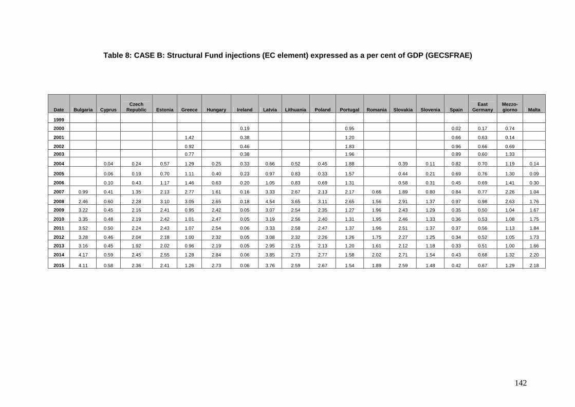
142
Table 8: CASE B: Structural Fund injections (EC element) expressed as a per cent of GDP (GECSFRAE)
Date Bulgaria Cyprus Czech
Republic Estonia Greece Hungary Ireland Latvia Lithuania Poland Portugal Romania Slovakia Slovenia Spain East
Germany Mezzo- giorno Malta
1999
2000 0.19 0.95 0.02 0.17 0.74
2001 1.42 0.38 1.20 0.66 0.63 0.14
2002 0.92 0.46 1.83 0.96 0.66 0.69 2003 0.77 0.38 1.96 0.89 0.60 1.33
2004 0.04 0.24 0.57 1.29 0.25 0.33 0.66 0.52 0.45 1.88 0.39 0.11 0.82 0.70 1.19 0.14
2005 0.06 0.19 0.70 1.11 0.40 0.23 0.97 0.83 0.33 1.57 0.44 0.21 0.69 0.76 1.30 0.09
2006 0.10 0.43 1.17 1.46 0.63 0.20 1.05 0.83 0.69 1.31 0.58 0.31 0.45 0.69 1.41 0.30
2007 0.99 0.41 1.35 2.13 2.77 1.61 0.16 3.33 2.67 2.13 2.17 0.66 1.89 0.80 0.84 0.77 2.26 1.04
2008 2.46 0.60 2.28 3.10 3.05 2.65 0.18 4.54 3.65 3.11 2.65 1.56 2.91 1.37 0.97 0.98 2.63 1.76
2009 3.22 0.45 2.16 2.41 0.95 2.42 0.05 3.07 2.54 2.35 1.27 1.96 2.43 1.29 0.35 0.50 1.04 1.67
2010 3.35 0.48 2.19 2.42 1.01 2.47 0.05 3.19 2.56 2.40 1.31 1.95 2.46 1.33 0.36 0.53 1.08 1.75
2011 3.52 0.50 2.24 2.43 1.07 2.54 0.06 3.33 2.58 2.47 1.37 1.96 2.51 1.37 0.37 0.56 1.13 1.84
2012 3.28 0.46 2.04 2.18 1.00 2.32 0.05 3.08 2.32 2.26 1.26 1.75 2.27 1.25 0.34 0.52 1.05 1.73
2013 3.16 0.45 1.92 2.02 0.96 2.19 0.05 2.95 2.15 2.13 1.20 1.61 2.12 1.18 0.33 0.51 1.00 1.66
2014 4.17 0.59 2.45 2.55 1.28 2.84 0.06 3.85 2.73 2.77 1.58 2.02 2.71 1.54 0.43 0.68 1.32 2.20
2015 4.11 0.58 2.36 2.41 1.26 2.73 0.06 3.76 2.59 2.67 1.54 1.89 2.59 1.48 0.42 0.67 1.29 2.18

143
Table 9: CASE B: Cumulated injections of Structural Funds (EC element). expressed as a percentage of GDP
Date Bulgaria Cyprus Czech
Republic Estonia Greece Hungary Ireland Latvia Lithuania Poland Portugal Romania Slovakia Slovenia Spain East
Germany Mezzo-giorno Malta
1999 0.00 0.00 0.00 0.00 0.00 0.00
2000 0.00 0.19 0.95 0.02 0.17 0.74
2001 1.42 0.57 2.16 0.69 0.80 0.87
2002 2.35 1.02 3.98 1.64 1.46 1.56
2003 0.00 0.00 0.00 0.00 3.12 0.00 1.40 0.00 0.00 0.00 5.94 0.00 0.00 2.53 2.06 2.90 0.00
2004 0.00 0.04 0.24 0.57 4.41 0.25 1.73 0.66 0.52 0.45 7.82 0.39 0.11 3.36 2.76 4.09 0.14
2005 0.00 0.10 0.42 1.27 5.51 0.65 1.97 1.63 1.34 0.78 9.39 0.83 0.32 4.05 3.52 5.39 0.23
2006 0.00 0.20 0.85 2.43 6.97 1.28 2.17 2.68 2.17 1.47 10.70 0.00 1.42 0.63 4.50 4.21 6.80 0.52
2007 0.99 0.61 2.21 4.56 9.74 2.89 2.33 6.01 4.84 3.60 12.87 0.66 3.31 1.44 5.34 4.98 9.06 1.56
2008 3.45 1.21 4.49 7.66 12.79 5.54 2.52 10.55 8.49 6.70 15.52 2.22 6.22 2.81 6.31 5.95 11.69 3.32
2009 6.67 1.66 6.66 10.08 13.74 7.96 2.57 13.62 11.03 9.05 16.79 4.18 8.65 4.10 6.66 6.46 12.73 5.00
2010 10.02 2.14 8.85 12.49 14.75 10.43 2.62 16.81 13.59 11.45 18.10 6.14 11.11 5.43 7.01 6.99 13.81 6.74
2011 13.54 2.63 11.09 14.92 15.82 12.97 2.68 20.13 16.17 13.92 19.46 8.09 13.61 6.79 7.39 7.54 14.94 8.59
2012 16.82 3.10 13.13 17.10 16.82 15.30 2.73 23.22 18.49 16.18 20.73 9.84 15.88 8.04 7.73 8.07 15.99 10.31
2013 19.98 3.54 15.05 19.12 17.78 17.49 2.78 26.17 20.64 18.31 21.93 11.45 18.00 9.22 8.06 8.58 16.99 11.97
2014 24.15 4.13 17.50 21.67 19.06 20.32 2.84 30.02 23.38 21.07 23.51 13.47 20.71 10.76 8.49 9.26 18.31 14.17
2015 28.26 4.72 19.86 24.08 20.32 23.05 2.90 33.78 25.96 23.75 25.05 15.36 23.30 12.24 8.91 9.93 19.60 16.35
2016 28.26 4.72 19.86 24.08 20.32 23.05 2.90 33.78 25.96 23.75 25.05 15.36 23.30 12.24 8.91 9.93 19.60 16.35
2017 28.26 4.72 19.86 24.08 20.32 23.05 2.90 33.78 25.96 23.75 25.05 15.36 23.30 12.24 8.91 9.93 19.60 16.35
2018 28.26 4.72 19.86 24.08 20.32 23.05 2.90 33.78 25.96 23.75 25.05 15.36 23.30 12.24 8.91 9.93 19.60 16.35
2019 28.26 4.72 19.86 24.08 20.32 23.05 2.90 33.78 25.96 23.75 25.05 15.36 23.30 12.24 8.91 9.93 19.60 16.35
2020 28.26 4.72 19.86 24.08 20.32 23.05 2.90 33.78 25.96 23.75 25.05 15.36 23.30 12.24 8.91 9.93 19.60 16.35

144
Table 10: CASE B: Percentage increase in the level of GDP. due to the Structural Funds (EC element)
Date Bulgaria Cyprus Czech
Republic Estonia Greece Hungary Ireland Latvia Lithuania Poland Portugal Romania Slovakia Slovenia Spain East
Germany Mezzo-giorno Malta
1999 0.00 0.00 0.00 0.00 0.00 0.00
2000 0.00 0.25 0.77 0.03 0.16 0.53
2001 1.74 0.57 1.01 0.78 0.61 0.03
2002 1.15 0.80 1.69 1.22 0.68 0.50 2003 0.00 0.00 0.00 0.00 1.08 0.00 0.83 0.00 0.00 0.00 1.99 0.00 0.00 1.26 0.66 0.98 0.00
2004 0.00 0.04 0.42 0.69 1.91 0.21 0.89 0.76 0.56 0.26 2.14 0.39 0.10 1.28 0.81 0.85 0.16
2005 0.00 0.07 0.36 0.95 2.14 0.36 0.89 1.25 1.02 0.24 2.10 0.48 0.20 1.22 0.92 0.98 0.11
2006 0.00 0.12 0.86 1.77 2.77 0.62 0.87 1.56 1.21 0.54 1.97 0.00 0.70 0.31 0.98 0.88 1.09 0.38
2007 0.67 0.48 2.78 3.50 4.89 1.63 0.83 4.90 3.84 1.69 2.91 0.79 2.25 0.83 1.48 0.99 1.83 1.35
2008 1.87 0.77 5.18 5.78 5.63 2.96 0.87 7.50 6.10 2.93 3.54 2.28 3.89 1.51 1.74 1.25 2.13 2.45
2009 2.74 0.68 5.56 5.57 2.68 3.14 0.68 6.18 5.44 2.93 2.36 3.43 3.87 1.58 1.07 0.79 0.78 2.53
2010 3.27 0.75 6.17 6.12 2.80 3.53 0.66 6.70 5.96 3.36 2.53 4.18 4.29 1.74 1.06 0.82 1.00 2.86
2011 3.81 0.83 6.81 6.68 2.89 3.93 0.65 7.26 6.47 3.81 2.63 4.93 4.71 1.90 1.09 0.87 1.13 3.20
2012 4.08 0.84 6.91 6.80 2.85 4.07 0.64 7.30 6.58 4.04 2.61 5.37 4.79 1.90 1.07 0.85 1.14 3.25
2013 4.39 0.86 7.10 6.98 2.85 4.25 0.62 7.42 6.76 4.30 2.62 5.81 4.92 1.93 1.06 0.85 1.16 3.37
2014 5.47 1.07 8.69 8.28 3.40 5.11 0.64 9.01 7.95 5.08 3.08 6.98 5.87 2.39 1.21 1.06 1.48 4.32 2015 5.94 1.12 9.05 8.65 3.45 5.40 0.63 9.33 8.27 5.44 3.12 7.60 6.10 2.47 1.24 1.08 1.46 4.50
2016 3.63 0.49 4.56 5.07 1.52 3.36 0.53 4.38 5.05 3.91 1.64 5.58 3.48 1.07 0.72 0.34 0.35 1.61
2017 3.52 0.44 4.38 4.71 1.45 3.26 0.51 4.05 4.81 3.82 1.64 5.32 3.28 1.01 0.66 0.31 0.51 1.72
2018 3.40 0.41 4.22 4.45 1.37 3.16 0.49 3.81 4.59 3.72 1.57 5.13 3.09 0.96 0.63 0.30 0.57 1.61
2019 3.31 0.39 4.07 4.27 1.32 3.06 0.47 3.64 4.43 3.63 1.53 4.95 2.95 0.93 0.61 0.29 0.61 1.55
2020 3.21 0.38 3.93 4.11 1.27 2.97 0.45 3.47 4.27 3.53 1.49 4.78 2.81 0.89 0.59 0.28 0.61 1.49

145
Table 11: CASE B: Cumulative percentage increase in the level of GDP. due to the Structural Funds (EC element)
Date Bulgaria Cyprus Czech
Republic Estonia Greece Hungary Ireland Latvia Lithuania Poland Portugal Romania Slovakia Slovenia Spain East
Germany Mezzo-giorno Malta
1999 0.00 0.00 0.00 0.00 0.00 0.00
2000 0.00 0.25 0.77 0.03 0.16 0.53
2001 1.74 0.83 1.79 0.80 0.77 0.56
2002 2.89 1.62 3.48 2.03 1.45 1.06
2003 0.00 0.00 0.00 0.00 3.98 0.00 2.46 0.00 0.00 0.00 5.47 0.00 0.00 3.28 2.11 2.04 0.00
2004 0.00 0.04 0.42 0.69 5.89 0.21 3.34 0.76 0.56 0.26 7.61 0.39 0.10 4.57 2.92 2.89 0.16
2005 0.00 0.11 0.77 1.64 8.03 0.57 4.23 2.01 1.58 0.50 9.71 0.86 0.30 5.79 3.84 3.87 0.26
2006 0.00 0.23 1.63 3.40 10.79 1.20 5.10 3.57 2.79 1.04 11.69 0.00 1.56 0.61 6.78 4.72 4.96 0.64
2007 0.67 0.70 4.41 6.90 15.68 2.82 5.92 8.47 6.63 2.73 14.60 0.79 3.81 1.45 8.26 5.71 6.79 1.99
2008 2.55 1.47 9.59 12.68 21.31 5.78 6.79 15.97 12.73 5.66 18.14 3.07 7.70 2.96 10.00 6.97 8.92 4.45
2009 5.29 2.15 15.15 18.26 23.99 8.92 7.47 22.14 18.17 8.59 20.50 6.50 11.57 4.54 11.07 7.75 9.70 6.98
2010 8.56 2.91 21.32 24.38 26.79 12.45 8.13 28.84 24.13 11.96 23.03 10.69 15.85 6.27 12.13 8.57 10.69 9.84
2011 12.37 3.73 28.13 31.06 29.68 16.38 8.79 36.10 30.60 15.77 25.66 15.62 20.56 8.17 13.22 9.45 11.83 13.04
2012 16.45 4.57 35.04 37.86 32.54 20.45 9.42 43.40 37.18 19.81 28.27 20.99 25.35 10.06 14.29 10.30 12.97 16.29
2013 20.85 5.43 42.15 44.84 35.39 24.69 10.05 50.82 43.94 24.11 30.89 26.80 30.27 11.99 15.35 11.15 14.13 19.66
2014 26.32 6.50 50.83 53.12 38.79 29.80 10.69 59.84 51.89 29.19 33.97 33.78 36.14 14.38 16.57 12.21 15.60 23.98
2015 32.26 7.62 59.88 61.77 42.24 35.20 11.32 69.17 60.16 34.62 37.09 41.38 42.25 16.85 17.80 13.29 17.06 28.48
2016 35.89 8.10 64.44 66.83 43.76 38.56 11.86 73.55 65.21 38.53 38.73 46.96 45.73 17.92 18.52 13.63 17.41 30.09
2017 39.41 8.55 68.82 71.54 45.22 41.82 12.37 77.60 70.03 42.35 40.37 52.28 49.01 18.93 19.18 13.95 17.92 31.81
2018 42.82 8.96 73.04 76.00 46.58 44.98 12.86 81.41 74.62 46.07 41.94 57.40 52.10 19.90 19.81 14.25 18.50 33.43
2019 46.12 9.36 77.11 80.27 47.91 48.04 13.33 85.05 79.05 49.70 43.47 62.36 55.05 20.82 20.42 14.54 19.11 34.98
2020 49.33 9.73 81.04 84.37 49.18 51.01 13.78 88.52 83.32 53.23 44.96 67.14 57.85 21.71 21.00 14.83 19.71 36.48

146
Table 12: CASE B: Cumulative Structural Fund multiplier (see text for definition)
Date Bulgaria Cyprus Czech
Republic Estonia Greece Hungary Ireland Latvia Lithuania Poland Portugal Romania Slovakia Slovenia Spain East
Germany Mezzo-giorno Malta
1999 0.00 0.00 0.00 0.00 0.00 0.00
2000 0.00 0.00 0.00 0.00 0.93 0.72
2001 1.22 1.45 0.83 1.17 0.97 0.64
2002 1.23 1.58 0.87 1.23 1.00 0.68
2003 0.00 0.00 0.00 0.00 1.28 0.00 1.75 0.00 0.00 0.00 0.92 0.00 0.00 1.30 1.03 0.70 0.00
2004 0.00 1.05 1.75 1.20 1.34 0.84 1.93 1.16 1.09 0.58 0.97 0.99 0.91 1.36 1.06 0.71 1.15
2005 0.00 1.08 1.82 1.29 1.46 0.88 2.15 1.24 1.17 0.64 1.03 1.04 0.94 1.43 1.09 0.72 1.16
2006 0.00 1.13 1.91 1.40 1.55 0.93 2.35 1.33 1.28 0.71 1.09 0.00 1.10 0.97 1.51 1.12 0.73 1.22
2007 0.68 1.15 2.00 1.51 1.61 0.98 2.54 1.41 1.37 0.76 1.13 1.20 1.15 1.01 1.55 1.15 0.75 1.28
2008 0.74 1.21 2.14 1.65 1.67 1.04 2.70 1.51 1.50 0.84 1.17 1.38 1.24 1.05 1.58 1.17 0.76 1.34
2009 0.79 1.29 2.28 1.81 1.75 1.12 2.91 1.63 1.65 0.95 1.22 1.55 1.34 1.11 1.66 1.20 0.76 1.40
2010 0.85 1.36 2.41 1.95 1.82 1.19 3.10 1.72 1.78 1.04 1.27 1.74 1.43 1.16 1.73 1.23 0.77 1.46
2011 0.91 1.42 2.54 2.08 1.88 1.26 3.28 1.79 1.89 1.13 1.32 1.93 1.51 1.20 1.79 1.25 0.79 1.52
2012 0.98 1.48 2.67 2.21 1.93 1.34 3.46 1.87 2.01 1.22 1.36 2.13 1.60 1.25 1.85 1.28 0.81 1.58
2013 1.04 1.53 2.80 2.35 1.99 1.41 3.62 1.94 2.13 1.32 1.41 2.34 1.68 1.30 1.91 1.30 0.83 1.64
2014 1.09 1.57 2.90 2.45 2.04 1.47 3.76 1.99 2.22 1.38 1.44 2.51 1.74 1.34 1.95 1.32 0.85 1.69
2015 1.14 1.61 3.02 2.56 2.08 1.53 3.90 2.05 2.32 1.46 1.48 2.69 1.81 1.38 2.00 1.34 0.87 1.74
2016 1.27 1.72 3.25 2.78 2.15 1.67 4.08 2.18 2.51 1.62 1.55 3.06 1.96 1.46 2.08 1.37 0.89 1.84
2017 1.39 1.81 3.47 2.97 2.23 1.81 4.26 2.30 2.70 1.78 1.61 3.40 2.10 1.55 2.15 1.40 0.91 1.95
2018 1.52 1.90 3.68 3.16 2.29 1.95 4.43 2.41 2.87 1.94 1.67 3.74 2.24 1.63 2.22 1.43 0.94 2.04
2019 1.63 1.98 3.88 3.33 2.36 2.08 4.59 2.52 3.04 2.09 1.74 4.06 2.36 1.70 2.29 1.46 0.97 2.14
2020 1.75 2.06 4.08 3.50 2.42 2.21 4.75 2.62 3.21 2.24 1.79 4.37 2.48 1.77 2.36 1.49 1.01 2.23

147
Table 13: CASE B: Impact of the Structural Fund on selected target variables in 2015
GDPM_pdif L_pdif L_dif Bulgaria 5.94 3.22 90.38 Cyprus 1.12 0.86 3.10
Czech Republic 9.05 7.14 327.83 Estonia 8.65 5.43 31.00 Greece 3.45 2.33 95.01
Hungary 5.40 3.73 147.29 Ireland 0.63 0.43 8.18 Latvia 9.33 5.98 55.43
Lithuania 8.27 4.81 67.67 Poland 5.44 2.80 384.21
Portugal 3.12 2.09 104.76 Romania 7.60 3.22 267.46 Slovakia 6.10 3.97 87.92 Slovenia 2.47 1.69 15.75
Spain 1.24 0.82 156.65 East Germany 1.08 0.88 59.98 Mezzogiorno 1.46 0.88 60.07
Malta 4.50 3.99 6.92
Total 1969.61

148
Table 14: CASE B: Impact of the Structural Fund on selected target variables in 2020 (long-run effects)
GDPM_pdif L_pdif L_dif
Bulgaria 3.21 1.16 32.15 Cyprus 0.38 0.15 0.54
Czech Republic 3.93 2.33 104.12 Estonia 4.11 1.98 11.29 Greece 1.27 0.57 23.26
Hungary 2.97 1.25 50.36 Ireland 0.45 0.27 5.25 Latvia 3.47 1.45 13.24
Lithuania 4.27 1.81 25.51 Poland 3.53 1.17 168.43
Portugal 1.49 0.66 33.19 Romania 4.78 1.74 147.99 Slovakia 2.81 1.26 29.15 Slovenia 0.89 0.34 3.24
Spain 0.59 0.26 51.03 East Germany 0.28 0.13 8.41
Mezzogiorno 0.61 0.14 9.82 Malta 1.49 1.04 1.89
Total 718.86

149
Part III
Installing the COHESION System

150
[11] COHESION System software requirements
11.1 Introductory remarks There are two main approaches to developing software for economic models, or systems of models. Option 1: In this case one designs and writes special programs to implement the database and model simulation system using any of a range of basic (or low level) programming languages such as FORTRAN or PASCAL. For example, this is the approach taken by the London-based National Institute for Economic and Social Research (NIESR) for their NiGEM global model as well as for NiDOM, their domestic model of the UK economy. Such an approach has both advantages and disadvantages. However, the contract upon which the development of the COHESION System was based effectively eliminated this option, since the Commission services required all model-related software to be completely based on standard and widely available software packages. Option 2: In this case one programs and implements the required database and model simulation system using high level, industry standard software packages. Examples of such packages include Microsoft Excel (for spreadsheets); TSP or Eviews (for database and econometric work); and WINSOLVE (for model simulations). The earlier work on the individual HERMIN national and regional models always followed this second option, and the practice was carried forward and extended for the development and implementation of the COHESION System. This approach was also in keeping with the contractual conditions set out by the Commission for the development of the system of models. Given the very complex array of tasks involved in developing, updating and running a system of economic models, one needs to draw on a range of specific software packages, each handling functionally different tasks. The software packages listed below are used to implement and apply the COHESION System of EU member state and regional models. (i) Text Editor: A text editor is needed to prepare text/data files for use as inputs to
other software (e.g., TSP and WINSOLVE). One can also make use of Microsoft Word, but restricting it to editing and saving “TXT” (i.e., ASCII) files. But the simpler Microsoft WordPad is perfectly adequate. Other more sophisticated text editors (like TextPad) can also be used.
(ii) Spreadsheet Software: Microsoft Excel is used to handle spreadsheets in
preparing the data, and in working with output tables generated from the WINSOLVE model simulation report generator. However, it should be noted that some econometric packages read and save spreadsheets using the older Lotus WK1 format, but these can always be read and saved using Excel. In the case of the TSP package, it only reads and writes the older format of XLS file, which does not permit multiple worksheets in a spreadsheet. In other words, one should

151
always save such spreadsheet files as (say) “version 4” of Excel 95, an option that is available in Microsoft Office 97 and 2003.80
(iii) Econometric Software: The development of databases and execution of
econometric tasks requires an econometric package which also has good database features for use in computerising all input data, and for carrying out the model calibration exercises. Potentially, there is a wide range of possibilities here. The earlier HERMIN-related research had always standardised on the TSP package (Time Series Processor), but this could be replaced by any of the modern packages (like EViews). The reason for using TSP rather than EViews is that TSP has a much simpler batch file language. It is highly desirable when developing and operating relatively large-scale macro models to do so using pre-prepared batch files. EViews has powerful interactive commands, and is excellent for developing and simulating small-scale “academic” models. But experience suggests that TSP is simpler in batch mode and hence preferable for use in the COHESION System.
(iv) Model Simulation Software: In an ideal world, the three main database,
econometric and model simulation tasks would be combined within a single package. For example, EViews and TSP can formally do all three tasks, at least for small-scale, manageable models. In practice, our experience has been that the simulation task is very specialised, particularly when large-scale models have to be operated on a routine basis by staff who are not econometric and modelling research specialists. Early work on the HERMIN model was carried out using TROLL on an IBM mainframe, but this was excessively expensive and subsequent port of TROLL to desktop PCs was complex and also expensive.81 Subsequently a shift was made to SIMPC, a DOS-based simulation package developed by the Dutch Central Plan Bureau. All the early HERMIN models were implemented using Excel+TSP+SIMPC. But as Windows became the dominant PC operating system in the mid-1990s, and full Windows integration of all software became mandatory, a second shift was made to Excel+TSP+WINSOLVE. WINSOLVE is a very sophisticated model simulation package that was originally developed by Richard Pearse for the Bank of England, and is now available commercially (www.econ.surrey.ac.uk/winsolve/). It is specifically designed for users who need to operate relatively large-scale policy models, and who need to carry out a wide range of different types of forecasting and policy analysis exercises on a routine basis.
11.2 Using the COHESION System software in practice In what follows, we describe how the computer system to implement the COHESION System was designed. In the longer run, as the COHESION System and its supporting databases stabilise, consideration could be given to designing a “turn-key” software package that completely insulated the user from any of the technical aspects that we are about to describe. However, this is not yet possible, and even when it is possible, it may not ever be desirable, for the following reasons:
80 It should be noted that the latest version of MS Excel in Office 2007 only permits one to save as Excel 95,
version 5. This can also be read by TSP and WINSOLVE, provided that only one worksheet is included in the spreadsheet.
81 On a mundane, practical note, the authorities in the new member states simply could not afford the high annual licence cost of TROLL. This, together with a desire for robustness and simplicity, was what pointed the HERMIN work in the direction of TSP and WINSOLVE.

152
i. Economic models – particularly models of post-transition, new EU member states – will continue to display instabilities and structural changes for some time to come. There are huge conceptual and practical differences between modelling (say) the French or German economies, and modelling the economies of Bulgaria and Romania. Even the more advanced new member states, such as Slovenia, Estonia, and the Czech Republic, are undergoing continual structural change. Consequently, such models have to be checked, upgraded and revised continually in ways that would make it difficult, even impossible, to standardise the COHESION System in the way that, say, an airline reservation system can be standardised.
ii. Even the data situation in the new member states is in a continual state of flux,
and examination of the AMECO database shows that data coverage is not always uniform or complete, even in the very recent years. In addition, the AMECO database system of DG-ECFIN is also in a state of continual upgrading, as more data are added.
iii. It is advisable that any user of an economic model be continually exposed to the
complexities of economic modelling, since all models – QUEST, MULTIMOD, HERMIN – have their imperfections and breakdowns. An unsuspecting user, operating in a mode which is insulated from detail by a standard, menu-driven, user interface, runs the risk of not noticing that the model is performing erratically, and may be led into making serious errors in policy analysis and forecasting.
The overall COHESION System is illustrated in Figure 11.1. In what follows we give outline details of the system, and hold off giving complete, technical details until later chapters. With a broad understanding of the general organisation of the system, it will be easier to develop a deeper and more technical knowledge of the detailed files that are needed to implement and run the complete COHESION System. Stage 1: Database of international time series, generated from AMECO A standard set of international variables drawn from those available in EUROSTAT is extracted either from the AMECO historical database (at the stage of model construction or updating) or from a AMECO-based forecasts (in the case of constructing baselines for cohesion policy impact simulations). The entire international coverage of AMECO is used, even though the system actually only draws on a subset of trading partners in practice. Scope for continual extension of the model is anticipated (e.g., to embrace the impact of economies such as China and India), so the entire AMECO international coverage is potentially available. Standardised Excel spreadsheets are produced to process the data copied over from AMECO, which are then read by the TSP software (in the case of model construction or updating), or by the WINSOLVE program (in the case of model policy simulations). This task, once set up, will normally only have to be performed once per year, when the model database is updated. All of the national HERMIN models make use of the same set of data on the global economy, even if the individual models make different selections of major trading partners. Stage 2: Databases for the country and macro-regional sub-models of the COHESION System Each country and macro-regional model has its own Excel spreadsheet inputs that consists of the minimal dataset that must be extracted and computerised from

153
AMECO/EUROSTAT sources, augmented, where absolutely necessary, by local Central Statistics Offices. Once this is set up, it only has to be altered once every year at the time of model system updating. The specific time of updating will be largely determined by the updating schedule of the AMECO database, which is currently twice each year – Spring and Autumn. Stage 3: Automatic generation of “derived” data for country and macro-regional sub-models of the COHESION System, using the minimal datasets from Stage 2 Each country and macro-regional model has its “data generation” batch files, developed in TSP batch language. These files are written in TSP batch language, and use as inputs the “minimal” datasets from Stage 2 above. They generate as output all the remaining data needed in the country and regional models. These data generation batch files will normally only be run once every year, and can be used to produce as output the full country and macro-regional model database of all variables needed in the model (i.e., the minimal input data plus all generated data). Although this model database is developed for use in calibrating and running the HERMIN models, it is of interest in its own right, since it is a detailed and highly structured macro database of countries that do not always have such data available in easily accessible format. Stage 4: Calibration of the country-model behavioural equations A set of standard files is set up (using TSP batch language) for each country and macro-regional sub-model. These files can be used to calibrate all the behavioural equations in a model. This task will normally be run only once every year, immediately after the model databases have been fully updated. As well as updating the behavioural coefficients routinely, care is also taken to ensure that none of the previous versions of any behavioural equation have “broken down” (i.e., failing to produce satisfactory results when re-estimated using the previous year’s equation formulation, but now making use of the new data set). After any such re-calibration exercise, two different outcomes can arise: Outcome 1: The re-estimation may be acceptable, and the behavioural equations simply require new (modified) numerical parameters. In this case, the new parameters are transferred manually to the model program file (i.e., the WINSOLVE version of the model equations). This model program file is always named HZZ5.TXT, and is a text file, where the letters ZZ are used to designate the two-character country code as used also within the AMECO database system. Outcome 2: Visual examination of the re-calibration results may suggest that some equations have broken down and require re-specification as well as re-estimation. In a situation where a completely new equation has had to be substituted for the previous one, two further tasks will need to be carried out. First, the relevant behavioural equation in the WINSOLVE model listing (HZZ5.TXT) must be replaced by the new formulation. Second, the new behavioural parameters must be copied over to the model program file (HZZ5.TXT). In the event of Outcome 2, i.e., where at least one of the entire set of behavioural equations breaks down after the re-calibration exercise, a further complication can arise. If the re-specification of the equation can be done by making use of variables drawn from those that are already in the model databank, then only the equation specification and equation parameters have to be altered in the model file HZZ5.TXT. However, if the re-specification requires the use of any new variables, i.e., not already contained in the model database, then the database system would have to be altered and extended to

154
include the new variables. This would require detailed changes to a range of system files, and would require expert knowledge of the details of the COHESION System files.
Figure 11.1: The computer-based implementation of COHESION System

155
Stage 5: Implementation of the country sub-models in WINSOLVE The implementation of a country or macro-regional sub-model in WINSOLVE requires only two files. The first file – referred to as the model equation file – is a text file that contains all the equations of the model, and is annotated with many explanatory remarks (HZZ5.TXT). In Outcome 1 of Stage 4 (see above), the equations in the model file (HZZ5.TXT) will not have to be altered as a result of model up-dating. Only a very minor alteration to the numerical coefficients of the affected behavioural equations must be made. If Outcome 2 of Stage 4 (see above) arises, then both the algebraic formulation of the equation affected and the new parameters have to be updated.82 The second file – referred to as the model data file - contains all the historical (or within-sample) data needed for the simulation of the model over the full extent of the historical data period. This is called HZZ5.SDF, and is a specific binary data file generated within WINSOLVE (details of which will be provided in subsequent Chapters). In normal circumstances, the historical WINSOLVE model data file (HZZ5.SDF) will only need to be generated once every year. The data is transferred from the TSP country or regional database into WINSOLVE format in one simple operation, by means of Excel spreadsheets containing all the exogenous and endogenous variables needed by the model) that can be generated automatically from the TSP model database file, HZZ5DB.TLB. Stage 6: Within sample simulation and testing of the country or macro-regional model When a country or regional sub-model is first implemented, or when it has been updated in the annual cycle of revision, it must be simulated within sample to test its internal integrity. This can be done interactively using the WINSOLVE interactive menu system, but is best carried out using standardised batch simulation files (i.e., simple text files that contain sequences of WINSOLVE simulation commands). Using the WINSOLVE batch simulation file, the following standardised within-sample simulations can be carried out: (i) A “consistency-checking” simulation, where equations are examined one at a
time, and checks are made to see that the behavioural equations and the model identities have been correctly incorporated in the model file. This was described previously in Chapter 8.
(ii) A “static” simulation, where the model is automatically re-started every year (as
explained in Chapter 8). (iii) A “dynamic” simulation, where the model is started at the beginning of the data
sample, and simulated for the full within sample period (as explained in Chapter 8).
When these test simulations are completed and checked, the model is ready for use in preparing an out-of-sample projection for use as a baseline in policy analysis.
82 We make the simplifying assumption that the equation re-specification can be done using the
existing set of model variables, and that no new variables are needed. If this does not hold, the task becomes more complicated and needs expert knowledge to carry out.

156
Stage 7: Preparation of out-of-sample baseline projection and policy analysis Before any model-based analysis of cohesion policy impacts can be carried out, it is necessary to set up an out-of-sample baseline projection. This is also executed using a standardised, country-specific WINSOLVE batch simulation file, and the process is illustrated in Figure 11.2.
Figure 11.2: Schema for preparing a baseline projection
We briefly describe the stages involved in generating a baseline: (i) Forecasts of the international variables (carried out using EUROSTAT/AMECO,
and described in Stage 1 above) are converted automatically from the Excel spreadsheet into the relevant section of the WINSOLVE batch file. For years beyond 2009 (as of September, 2008), such forecasts need to be based on other sources, and on informed judgement, since AMECO usually only goes as far as the year 2009.
(ii) A standard set of domestic policy assumptions (excluding cohesion policy) is
made. Usually these take the form of simple projections of the policy variables from there last within-sample value. This has been described previously in Chapter 8.

157
(iii) A standard set of assumptions is made about all the remaining exogenous variables in the country or regional sub-model. These usually do not have to be changed much from year to year.
(iv) All the cohesion policy instruments are set at zero values.83 (v) Having generated the required changes to the contents of the WINSOLVE batch
projection file, it is run and the baseline projection is generated and the output presented in a routine report generator.
It should be noted that the baseline projection is, in effect, a medium-term forecast for the country whose model is being used. Although formally easy to describe, the process is one where a high degree of skill and country-specific knowledge is needed if the baseline projection is to be reasonably realistic. In addition, the baseline projections need to be “tuned”, i.e., examined for plausibility and for coherence with any other forecasts available within the Commission (e.g., those prepared by DG-ECFIN using QUEST, and the OECD, etc.). Once the baseline out-of-sample projection is acceptable, it can be used as a baseline for any subsequent policy shocks. It is very simple to set up policy shocks (other than for cohesion policy impact analysis) using the WINSOLVE batch language. A standard set of such shocks (e.g., using world demand (OWM), public employment (LG), public investment (IGV) and external prices (PWORLD, PM) are provided so that these diagnostic shocks can be easily executed. Two simulations (at a minimum) are needed to carry out a cohesion policy impact analysis. The first consists of the baseline projection, described above. The second requires the preparation of a specific WINSOLVE batch simulation file that incorporates all the required financial and other data that describe the nature of the cohesion policy being examined. Sample versions are prepared for each country and regional model, and can be easily adapted for a range of further cohesion policy simulations. The manner in which the cohesion policy instruments are incorporated into the COHESION System country and regional sub-models has been described in detail in Chapter 4 above. From the point of view of the computer system and its routine operation, the necessary simulations can be carried out using fully standardised WINSOLVE batch simulation files, and the results transferred either to a report generator customised within WINSOLVE, or to any other reporting system via MS Excel output files generated by WINSOLVE. However, such model output should never be used uncritically. Great care and attention needs to be paid to the interpretation of the output of such simulations.
83 Note that we make the simplifying assumption that the baseline projection is a “no cohesion
policy” baseline, i.e., all cohesion policy expenditure instruments are set to zero. This is the most appropriate assumption for use in ex-ante impact analysis. However, in mid-term and ex-post analysis, the historical data will contain the effects of cohesion policy. In such analysis, one usually switches to a “with cohesion policy” baseline, and the counterfactual simulation removes the cohesion policy instruments by re-setting them to zero.

158
[12] Setting up the HERMIN country model databases The objective of this chapter is to describe how a typical HERMIN country model database is set up. Such a database includes at least all the variables required to set up a HERMIN country model. But in addition, many useful extra variables are generated to assist in the exploration of the patterns of behaviour in the economy while the model system is being designed, calibrated and improved. For example, sectoral employment data are needed within a HERMIN country model for five production sectors: manufacturing (LT), market services (LM), building and construction (LB), agriculture (LA) and the public (or non-market) sector (LG). In order to check the validity, stability and accuracy of these five series, we also calculate the sectoral employment shares. Thus, if L represents total employment numbers, and LA is employment in agriculture, then we calculate LASHR as 100*(LA/L), i.e., the percentage share of employment in agriculture. Similarly, we calculate the other four sectoral employment shares. These “share” variables, together with a range of other variables, are not needed inside a HERMIN model, but are very useful when examining the raw data and describing evolving trends in the economy. However, at the stage where the data are transferred from the TSP database (which consists of a binary file called HZZ5DB.TLB), to the HERMIN/WINSOLVE model database (HZZ5.SDF), we select only the necessary and sufficient data for the model, i.e., the exact number of variables needed in the model, which is a subset of the entire country database HZZ5DB.TLB.
Three main stages are gone through in generating a country model database. In what follows, we use the database for the Estonian model (HEE5) as an illustrative example. But almost identical procedures are used in all of the 16 COHESION System country HERMIN models, where usually only the country designation “ZZ” changes in the file names and in the file contents.84 The remaining two regional models (i.e., East Germany (HGE5) and the Italian Mezzogiorno (HMZ4) are handled somewhat differently, since the input data needed cannot be standardised as much as for the country model (based, as the latter is mainly on officially published AMECO/EUROSTAT data).
Stage 1: The international data
The data for Stage 1 are generated using a TSP batch file called BASIC_AMECO_HEE5.TSP.85 In any file, the extension “TSP“ always denotes a TSP batch file, i.e., a sequence of TSP calculations that are carried out automatically when the batch file (or program) is executed.86 This TSP batch file reads in the necessary international data common to all the COHESION country models. This consists of data downloaded from the DG-ECFIN database system AMECO, and provides
i. Industrial output in a wide range of actual and potential trading partners;
ii. Total imports of a wide range of actual and potential trading partners
iii. The rate of unemployment in UK, as a proxy for an “alternative“ labour market 84 It should be noted that the economic variables in each HERMIN model do not contain any
country “identifiers”. In other words, the variable CONS is used in all models to represent real household consumption. The country identification comes from the sub-directory file nomenclature, and not from the variable names.
85 Thus, if we were describing the Polish model, the TSP file name would be BASIC_AMECO_HPL5.TSP 86 Although the file extension on a TSP batch file is “TSP”, it is an ASCII text file. If this file is
prepared using MS Word, it must always be saved as a TXT file, and not as a DOC file.

159
iv. A range of national exchange rates against the euro
The input data are in the form of an Excel file called BASIC_AMECO.XLS, which is contained in the Estonian model sub-directory, C:\SIMREGIO\HEE5. This XLS file (BASIC_AMECO.XLS) does not require any “EE” identifier, since an identical common set of international data is used in all country models. The XLS file is constructed directly from AMECO data, with a switch to a more transparent HERMIN-type variable notation. The conversion between AMECO notation and HERMIN notation will be explained in Chapter 15, where we describe how the AMECO data are extracted for processing by the TSP batch file, BASIC_AMECO_HEE5.TSP. This TSP batch file simply processes these input data and writes them out to a TSP binary database file called BASIC_AMECO.TLB. This process is illustrated below:
Reads BASIC_AMECO.XLS
BASIC_AMECO_HEE5.TSP
Generates BASIC_AMECO.TLB in the
SIMREGIO\HEE5 subdirectory
Stage 2: The country national accounts and related data
The second TSP batch file is called BASIC_OTHER_HEE5.TSP, and its task is to input a range of national accounting and other related data (for the case of Estonia in the illustrative example). Once again, the data come mainly from the AMECO database, suitably transformed and modified. But for some countries the AMECO database is not complete, and some required data are missing, even though the latest version of AMECO has been revised and extended in order to provide the full five-sector branch disaggregation that is needed in HERMIN. In cases of missing data the AMECO database is augmented by extra data, usually taken directly from EUROSTAT sources, e.g., the NACE-17 level branch data, where AMECO does not include them. The details will be set out in Chapter 15 below. In this stage, there are four data input files, in the form of four Excel input spreadsheets.
AMECO_Part01_HEE5.XLS: Standard national accounting data from AMECO
AMECO_Part02_HEE5.XLS: Public sector revenue and expenditure data from AMECO
AMECO_Part03_HEE5.XLS: NACE 5 branch data from AMECO and, where required, directly from EUROSTAT
Export_Shares_HEE5.XLS: Export share data from EUROSTAT (for Estonia in the illustrative case)
A series of data transformations are sometimes carried out within the TSP batch file BASIC_OTHER_HEE5.TSP, which generate other variables. The nature of these transformations is described in full detail in the annotations that are included in the

160
country-specific TSP batch files themselves. For example, AMECO gives data in billions of currency units, and this has to be transformed to the units of millions used in HERMIN.
When the first (March, 2007) version of the database was constructed, it was not possible – using AMECO alone – to split employment, GDP and wage bill data for total services, as given in the earlier version of AMECO, into its two components: market services (M) and non-market services (G), as required by HERMIN. In order to be able to do this, we had to make use of data series extracted directly from EUROSTAT at the NACE-17 branch level (specifically, NACE branches L, M and N), for employment, GDP at current and constant factor cost, and the wage bill.87
The sequence of calculations is illustrated in the diagram below, showing the TSP batch file, the four data input Excel files, and the generated TSP binary database file, BASIC_OTHER_HEE5.TLB
AMECO_Part01_HEE5.XLS AMECO_Part02_HEE5.XLS AMECO_Part03_HEE5.XLS Export_Shares_HEE5.XLS
BASIC_OTHER_HEE5.TSP
BASIC_OTHER_HEE5.TLB
Stage 3: A miscellaneous set of country data
Although AMECO/EUROSTAT sources provide a wide range of data that can be used in HERMIN, nevertheless, not all data required by the country models are available from either of these two sources. Two simple examples will illustrate this point. In the first example, AMECO provides data on total revenue from direct taxation (GTY, in HERMIN notation). But the HERMIN model needs to have total direct tax revenue further disaggregated into income tax paid directly by households (GTYPER) and corporation tax revenue that is paid by firms (GTYC).88 In the second example, the HERMIN model also needs to distinguish data on social insurance contributions paid by workers from contributions paid by employers. In both cases, the required split permits a more accurate definition of household disposable income. In both cases we need data from outside AMECO/EUROSTAT in order to make the required split. These are usually obtained from national sources, or – in the complete absence of local data – we make an approximation of the split.
The data generation process is shown in the diagram below. The TSP batch file, BASIC_MISCEL_HEE5.TSP reads in the data file BASIC_MISCEL_HEE5.XLS, which contains any miscellaneous data inputs that are required. The resulting transformed and augmented data are then written out to a TSP binary database file called BASIC_MISCEL_HEE5.TLB, as illustrated below.
87 In Chapter 12 we simply assume that the AMECO, EUROSTAT and other input data are available in spread-sheet form. Later, in Chapter 15 we will give complete information on how these data are actually derived from basic sources. 88 The split of GTY into GTYP and GTYC is required in order to construct a measure of household disposable income in the model. GTYC is paid by the company sector. Only GTYP is paid by the household sector.
reads
generates

161
BASIC_MISCEL_HEE5.XLS
BASIC_MISCEL_HEE5.TSP
BASIC_ MISCEL _HEE5.TLB
Stage 4: The generation of the complete national model database.
In this fourth and final stage, the three TSP binary database files generated in Stages 1-3 above are read into, and processed by the TSP program batch file, HERDATA_HEE5.TSP. This is the main data generation task and carries out very extensive processing. The data generation process is illustrated below. The three binary database input files are called BASIC_AMECO.TLB (international data, common to all country models); BASIC_OTHER_HEE5.TLB (national accounting data for a specific country, Estonia in this case), and the third file BASIC_MISCEL_HEE5.TLB (containing a small set of miscellaneous data that are not available in AMECO/Eurostat).
BASIC_AMECO_HEE5.TLB BASIC_MISCEL_HEE5.TLB BASIC_OTHER_HEE5.TLB
HERDATA_HEE5.TSP
HEE5DB.TLB
The final TSP binary database file that is generated – namely, HEE5DB.TLB, in the case of Estonia - is a comprehensive set of annual time series for Estonia, which is the main input database for the model database.
The TSP binary database file, HEE5DB.TLB, is the basic input to all subsequent stages of the installation of the COHESION System models. It is used in the calibration of the Estonian HERMIN model behavioural equations, as a source of historical data for input to the model simulation software (WINSOLVE), and more generally as a source of systematic data for a wide range of analysis of the economies of the countries which are in receipt of Structural and Cohesion Fund assistance.
A complete dictionary of the variables used in a typical HERMIN country model is provided in Annex A.2, where we list the exogenous and endogenous variables separately. The best way to examine and understand the nature of the variables is to use this annotated dictionary in conjunction with the model listing, which also contains extensive explanations of how the model uses these variables in the identities and behavioural equations.
reads
generates
reads
generates

162
[13] Calibrating the model behavioural equations The TSP software is used to carry out the calibration of the HERMIN model behavioural equations. The specifications of these equations has already been described in Chapter 3, and the results and interpretation of the calibration exercise has been described in Chapter 5. The purpose of this chapter is to describe the actual process used to carry out the calibration exercise. It should be stressed again that the eighteen economies being modelled (sixteen countries and two macro-regions) are all developing and undergoing structural change, both due to the impacts of cohesion policies and for many other reasons. In the case of most of the new member states, we only have available eleven annual data observations (1995-2005), since the pre-1989 data are inappropriate (coming from the Communist centrally planned period), and the 1989-1994 period was one of post-Communist turbulence and transition, and must be regarded as untypical of the recovery period of the liberal, market-based policy regime. The short data sample, combined with the rapid structural change of the post-1995 period, implies that the scope for formal econometric testing is extremely limited and almost non-existent. As explained in Chapter 5, we engage in a data calibration or “curve-fitting” exercise, and select parameter values that appear to be reasonable in view of the known features and characteristics of the economy in question. This calibration exercise can be carried out interactively using TSP, and initially such exploration (“data mining”) was performed. However, the lessons learned from the interactive exploration were then incorporated into a series of TSP batch files that re-execute the calibrations automatically and generate printed output that can be studied and used. The purpose of this Chapter is to describe the process of how the TSP batch files have been developed and used to calibrate the HERMIN country models. Stage 1: The model equation listing An overview of the behavioural and identity equations can be obtained from the listing of the model equations contained in the file HEE5.TXT (in the case of Estonia), a copy of which is contained in the annexes. This is an annotated version of the Estonian model file, where the meaning of all the equations (identities as well as behavioural equations) is carefully explained, and which includes the final values selected for all the calibrated behavioural equation parameters. We illustrate this by extracting the consumption function from the complete model listing, as follows: @ A "Permanent Income Hypothesis" (PIH) consumption function is specified. @ Consumers can be partially or totally liquidity constrained, as determined @ in the equation calibration. *P ACONS1 = -4.77495 ; *P ACONS2 = 0.708794 ; {SR impact MPC} *P ACONS3 = 0.0 ; {MPC out of wealth} *A CONS = ACONS1+ACONS2*YRPERD+ACONS3*WNH(-1) ; Any line starting with the symbol “@” is simply an explanatory comment, designed to assist the reader in understanding the meaning of the equation. The lines starting with

163
“*P” give numerical values of behavioural parameters. These are inserted manually from the TSP calibration output files to be described below.89 The line starting with “*A” designates that a behavioural equations will immediately follow. In the illustrative case of the consumption function, this is formulated in terms of a partial liquidity constraint. In the case of Estonia, no wealth effect could be calibrated (i.e., ACONS3 is zero). The crucial parameter ACONS2 is the so-called “marginal propensity to consume”, and was found to take the value 0.709. All the other behavioural equations in the model listing HEE5.TXT are described in a similar fashion, and the detailed results have already been described in Chapter 5. In the rest of this Chapter we describe the three TSP batch files that were used to calibrate the HERMIN country models. Stage 2: Calibrating the joint factor demand systems The “joint factor demand” system is an integrated set of two equations that determine labour and capital inputs, subject to a CES production function constraint. The theoretical derivations have been given previously in Chapter 3, with the calibration results in Chapter 5. The TSP batch file CALIB_JFDPC_HEE5.TSP is used to calibrate the joint factor demand system for the three sectors manufacturing (T), market services (M) and ), building and construction (B). This is illustrated below:
HEE5DB.TLB (input data)
CALIB_JFDPC_HEE5.TSP
CALIB_JFDPC_HEE5.OUT (calibration)
In other words, the TSP batch file CALIB_JFDPC_HEE5.TSP accesses the HERMIN country database (HEE5DB.TLB, in the case of Estonia) and produces an output file called CALIB_JFDPC_HEE5.OUT. This output file shows a series of calibrations, based on free estimation (i.e., no imposed parameter constraints) and for a series of three imposed values of the elasticity of substitution (σ) in the CES production function. The range of values includes σ=0.2 (quasi Leontief), σ=0.5 (mid way between Leontief and Cobb-Douglas), and σ=0.8 (quasi Cobb-Douglas). In the revised version of this batch file, for simplicity we only use the case of σ=0.5. Stage 3 : Calibration of the remaining behavioural equations One of the difficulties in relying on econometric calibration techniques for new member states is that there are not enough data observations to carry out formal hypothesis testing and structural stability analysis. A second difficulty is that many of these
89 In later versions of the COHESION System, the process of insertion of calibrated parameter values could be automated. But the relative instability of the data for some of the NMS makes this less attractive.
reads
outputs

164
economies are undergoing rapid structural change, rendering unreliable any calibration performed using a run of eleven years data.
Rather than use parameter values that may vary randomly over a wide spectrum, we carry out a final series of what we call “standardised” calibrations, for all models, and we try to ensure that the resulting properties of the calibrated equations are both reasonable (within a specific country model) and are also reasonable (across a series of economies that might reasonably be expected to share similar structural characteristics). This task is performed by the TSP batch file HEE5_Standardised_Calibration.TSP, as illustrated below;
HEE5DB.TLB (data input)
HEE5_Standardised_Calibration.TSP
HEE5_Standardised_Calibration.OUT (calibration)
Once again, the TSP batch file accesses the HERMIN country database, HEE5DB.TLB, and produces an output file, HEE5_Standardised_Calibration.OUT, from which the values of the calibrated parameters can be extracted for insertion into the model file, HEE5.TXT.
inputs
outputs

165
[14] Implementing, testing and running the models The WINSOLVE program is a sophisticated tool, specifically designed to facilitate the management and use of large-scale macro models. It can be used in two modes: interactive and batch. However, it is seldom advisable to use the interactive mode when the model being implemented is complex and large. Although initial exploratory work was carried out on the COHESION System country and regional models using the interactive mode of WINSOLVE, all routine use of the models is carried out though the medium of carefully designed and pre-written WINSOLVE batch simulation files. These are standard ASCII or text files that must always have the file extension LOG, e.g., the file HEE5_LG.LOG is a WINSOLVE batch simulation file that makes a shock to the exogenous variable LG (public employment). There is a sequence of four sets of WINSOLVE operations and related batch files needed to get to the final stage of executing an NSRF impact analysis. These files are as follows: Stage 1: Preparing the historical data for reading into WINSOLVE The first operation is carried out using the TSP batch file HIST_WINSOLVE_HEE5.TSP, and is used to dump all the data needed for the model HEE5 out to three XLS files for subsequent input to WINSOLVE, as illustrated below:
HEE5DB.TLB (data input)
HIST_WINSOLVE_HEE5.TSP
HEE5_EXOG.XLS HEE5_ENDOG1.XLS (XLS files generated) HEE5_ENDOG2.XLS
The country database binary file, HEE5DB.TLB is accessed, and the necessary and sufficient set of country model data is extracted and written out to the three generated XLS files. Note that WINSOLVE expects there to be a perfect, one-to-one match between the list of variables actually used in any specific country model and the set of data series input. If any variables needed by the model are missing, an error message will be generated. In there are any “surplus” variables in the set of XLS input files, an error message will also be generated. Three XLS data files are generated by running HIST_WINSOLVE_HEE5.TSP: HEE5_EXOG.XLS, HEE5_ENDOG1.XLS and HEE5_ENDOG2.XLS. The explanation for the need for these three files (rather than one) is as follows. First, it is useful to distinguish between exogenous and endogenous variables, particularly when we come later to carry out an out-of-sample projections. Second, Microsoft Excel imposes a restriction of 256 columns in any spreadsheet, and there are more than 256 endogenous variables. Consequently, we need to split them into two parts, making three files in total.90
90 The restriction to 256 columns has been removed in Office 2007. However, most users still only have access to Office 2003.
inputs
outputs

166
Note that some special requirements attach to these files. First, they need to be stored as Microsoft Excel, version 4.0, in order to be able to read them into WINSOLVE. Second, all references to “missing” data (#N/A in the initial Excel files) must be removed and replaced by some number (usually selected as zero). Third, the column that contains the identifiers for the year must be generated manually, taking account of the specific range of data. Stage 2: Inserting historical data into WINSOLVE Every time a new set of historical data is prepared (usually about once every year), these data must be input to WINSOLVE, using the three XLS files described in Stage 1. This is best carried out interactively, using the following sequence of steps. Step1: Execute WINSOLVE Step2: Load model file, HEE5.TXT Step3: Create a blank data set over 1995-2020 (NMS), 1980-2020
(OMS)91 Step4: Read each of the 3 XLS files generated from Stage 2 previously Step5: Save data in a file named HEE5.SDF Step 1 is performed simply by double clicking on the WINSOLVE icon located on the desktop. Step 2 is performed by clicking on the “open model” icon on the WINSOLVE menu. Step 3 is performed by using the “data” menu, and clicking on “create new data”. Use the subsequent menu to define an annual set of data, from 1995-2020 for the NMS models (1980-2020 for the OMS models). Do not initialise the data (as in the displayed menu). Step 4 is performed also by using the “data” menu, using the “open data” command. Use this to load each of the three XLS files HEE5_EXOG.XLS, HEE5_ENDOG1.XLS and HEE5_ENDOG2.XLS, with the new data overwriting the old (null) data. In step 5 the complete set of historical data can be stored permanently in a wide variety of formats. The generic WINSOLVE format (SDF) is preferable. Having saved the data in this format, as HEE5.SDF, one can simply read it in all subsequent simulations, until such times as it needs updating. Stage 3: Model simulations: Testing Phase Any newly constructed model should always be subjected to a wide range of diagnostic testing before it is ever used for “real” policy analysis simulations. The results of these tests have already been described previously, in Chapter 8. In this Chapter we simply list the sequence of pre-prepared WINSOLVE batch simulation files that can be used to test the model very simply. The case of Estonia is used as an example, but the same files are available for all the COHESION System models (replacing HEE5 by HZZ5). a) HEE5_RESIDUAL_CHECK.LOG: Carries out single equations residual check b) HEE5_PROJ1.LOG: Projects exogenous variables for 2005-2020 c) HEE5_PROJ2.LOG: Carries out model simulations out to 2020
91 We use the year 2020 as the terminal year for simulations. This permits simulations to continue for a
further seven years beyond 2013, the end of the current Structural Fund programme period. Of course only the data from the start of the sample to the end of the historical data period are actually available. Data beyond the historical sample4 is set automatically to zero.

167
(baseline) (HEE5_BASELINE.XLS) d) HEE5_OWM.LOG Shock to world demand e) HEE5_LG.LOG Shock to public employment f) HEE5_IGV.LOG Shock to public employment g) HEE5_PRICE.LOG Shock to all exogenous price variables h) HEE5_DEVALUATION.LOG Devaluation against Euro Test (a) is used to check that the historical data are compatible with the model identity and behavioural equations. It takes each equation in the model in isolation from all others, and inserts the historical data into the right-hand-side variables. The value of the left-hand-side variable, thus calculated, is then compared with the historical value of the left-hand-side variable. In the case of an identity, the differences should only be die to rounding errors. In the case of the behavioural equations, the differences should be the same as the stochastic residuals derived when the equations were calibrated. Test (b) is a WINSOLVE batch file that projects all the values of the model exogenous variables out from the end of the historical data sample (2005, in the present case), to 2020. This process was described in Chapter 9. The annexes contain examples of the required files. Test (c) is a WINSOLVE batch file that uses these projections of the exogenous variables to carry out a baseline simulation to the year 2020. The results, for a range of important macro-variables, are stored in the Excel file HEE5_BASELINE.SDF, for subsequent examination and use. Test (d) is used to shock the value of total imports in each of the main trading partners of the country whose model is being used. This tests the impact of a change in the external (world) environment on economic performance. Test (e) is used to shock numbers employed in the public sector, LG. No offsetting tax funding changes are implemented, although a balanced budget version would be simple to implement. Test (f) is used to shock the value of public investment, IGV.92 Test (g) is used to shock all exogenous price variables, to examine the role of price homogeneity in the models behavioural price determination systems. Test (h) examines the impact of a devaluation of the national currency against all external currencies, and resembles the price shock. Stage 4: NSRF policy impact simulations Four batch files have been prepared for each country, in order to examine NSRF impacts. These are referred to as CASE A, CASE B, CASE C and CASE D, and the corresponding WINSOLVE LOG files are called: HEE5_NSRF_A.LOG (Case A), HEE5_NSRF_B.LOG (Case B),
92 Note that in test (f), there are no spillover mechanisms. In other words, this is a purely Keynesian shoc to demand.

168
HEE5_NSRF_C.LOG (Case C) and HEE5_NSRF_D.LOG (Case D). Their use is illustrated below:
HEE5_NSRF_A.LOG Estonia_NSRF_A_Impacts.XLS
HEE5_NSRF_B.LOG Estonia_NSRF_B_Impacts.XLS
HEE5_NSRF_C.LOG Estonia_NSRF_C_Impacts.XLS
HEE5_NSRF_D.LOG Estonia_NSRF_D_Impacts.XLS
In addition to running the NSRF simulation, these LOG files automatically generate an Excel file as output, listing the impacts of the NSRF on a wide range of target macro indicators. These impacts have already been examined and described in Chapter 10. The list can have any of the models variables, endogenous and exogenous. In a specific study, one can design a set of standard output indicators and have them generated automatically. Of course, it is always possible to augment the standard data dump with an interactive exploration of the impacts on other variables, and generate ad-hoc tables, graphs and spreadsheets.
generates

169
[15] Data sources and data generation In the previous three chapters we described the system of Excel, TSP and WINSOLVE batch files that have been set up to service the data collection, data generation, model calibration and model simulation requirements of the new COHESION System of HERMIN country and regional models. In this chapter we first describe a series of background files that are required for use as inputs to the data generation process for the individual country models. These files are of a highly technical nature, and are intended for use only by experienced analysts who need to work directly with the detail of the data and of the models and who are already totally familiar with the previous set of files. Stages 1-4 are the top level files. In Stage 5 we describe how the data for a specific country model are prepared, using the Estonian case as an example. In Stage 6 we describe the final part of the production of a country HERMIN database, namely inputting the “raw” data, and generating all the remaining data. These six stages are explained below in more detail. In Stage 1 we describe how the original NSRF data are extracted from the Financial Tables and other sources and transformed for use in the HERMIN NSRF impact simulations. Since this process is not completely standardised, and changes between member states and over time, the examples that we use are merely designed to illustrate the process of NDP/NSRF data collection. This data collection system will have to be adapted to changing circumstances. In Stage 2 we describe more precisely how raw data are extracted from AMECO and prepared for use in generating all of the individual HERMIN country databases, i.e., the TSP binary database file HZZ5DB.TLB. This was illustrated using the Estonian case, HEE5DB.TLB, in Chapter 12 above. In Stage 3 we describe how some additional sectoral national accounting data for certain countries have to be extracted directly from EUROSTAT and other sources. This arises because of the requirement to separate the public service sector (G) from the aggregate services sector (private (M) plus public (G)) in cases where this division is not yet available in AMECO.93 Until the AMECO sectoral coverage is fully standardised, these ad-hoc operations will be required to build the COHESION System database. In Stage 4 we describe how data on export share by country of destination are collected. In Stage 5 we describe the extraction of data on expenditures on research and development (R&D). These data are used to construct a baseline historical series of a notional “stock” of R&D, for use in the spillover mechanism in the NSRF simulations. In Stage 6 we describe how the data in the previous five stages above are transferred into the individual country sub-directories for use in generating the databases for each country. This is a process that can be standardised only to a limited extent. But we make every effort to retain as high a degree of standardisation as possible. Departures from the standardised approach are clearly signalled. In Stage 7 we describe the process that is used to input all the “raw” data, drawn from the above five stages, and then “generates” all the remaining data using a country-specific TSP batch file called HERDATA_HZZ5.TSP (HERDATA_HEE5.TSP in the 93 As previously noted, the latest version of AMECO provides a disaggregation of all five HERMIN ISIS branches (T, M, B, A and G). However, data for the following countries are very deficient: BG, EL, HU, IE, MT, PT and RO. For these countries, we fall back on the version 1 (Spring, 2007) methodology.

170
illustrative case of Estonia). The output from this final stage in the TSP binary database file HZZ5DB.TLB (HEE5DB.TLB in the illuatrative case of Estonia), which contains all the data needed to assemble a HERMIN country model. Stage 1: Extracting the NSRF data The data for expenditures on NDP and/or NSRF investments are usually presented in a series of financial tables published in the official country NDP and/or NSRF documentation, and classified by Operational Programme (OP) and individual measures within each OP.94 A standardised Excel-based system has been designed to take these basic NSRF data and to reclassify them in terms of the three economic categories used in the HERMIN models, namely physical infrastructure (PI), human resources (HR) and direct aid to productive sectors (APS). Within the APS category, we also need to know the fraction of the total that is allocated to manufacturing (T), to market services (M) and to agriculture (A). Also, within the total of APS, we need to know the fraction that is allocated to funding of R&D actifities as distinct from other non-R&D aid. The subdirectory C:\SIMREGIO\AAA_NSRF_DATA_CONVERSION contains a full set of eighteen XLS files that carry out the above task for each of the models. For example, the XLS file that prepares the Estonian data is called NSRF_HEE5_Estonia.XLS. Note that the NSRF data extraction takes place in the special sub-directory C:\SIMREGIO\AAA_NSRF_DATA_CONVERSION, which stands above the individual sub-directories that handle activities for each separate country model. This special NSRF sub-directory is the source of data files for subsequent transfer to the individual country model sub-directories, as will be explained later. Comments and explanations are contained in these XLS files which describe their structure, and where the data are located. This is designed to assist in the subsequent extraction and incorporation of the required NSRF data into the relevant WINSOLVE LOG files for use in simulating the impacts of the NSRF policies. The different NSRF data configuration cases are set out in separate worksheets. For example, the file NSRF_HEE5_Estonia.XLS contains a worksheet called “NSRF EC data inputs (A)”. This worksheet contains the NSRF data for a specific set of NSRF data called “CASE A” for Estonia. Within this worksheet, the relevant data that will change from simulation to simulation (e.g., from CASE A to CASE D for the present XLS file) are as follows:
i. GECSFEC_E: The total EC contribution, in current euro, for the required period of years
ii. RDPCOFIN: The domestic public co-finance ratio
iii. RPRCOFIN: The domestic private co-finance ratio
iv. RIGVCSF: Investment allocations to physical infrastructure, expressed as a
percentage of total. The qualifiers E, D and P are used in the model to designate EC, domestic public and domestic private percentages. However, these are normally identical and only one of the three identical sets of data (RIGVCSF) is listed in the worksheet.
94 The change in name of the strategic Structural Fund documentation from National Development Plan (NDP) to National Strategic Reference Framework (NSRF) occurred during the switch to the present programming period (2007-2013). For simplicity, we will refer to NSRF, even in cases where NDP would be more accurate.

171
v. RGTRSF: Investment allocations to human resources, expressed as a percentage
of total. The qualifiers E, D and P are used in the model to designate EC, domestic public and domestic private percentages. However, these are normally identical and only one of the three identical sets of data (RGTRSF) is listed in the worksheet.
vi. RTRIT: Fractions of direct aid to firms allocated to manufacturing. The qualifiers E,
D and P are used in the model to designate EC, domestic public and domestic private percentages. However, these are normally identical and only one of the three identical sets of data (RTRIT) is listed in the worksheet.
vii. RTRIM: Fractions of direct aid to firms allocated to market services. The qualifiers
E, D and P are used in the model to designate EC, domestic public and domestic private percentages. However, these are normally identical and only one of the three identical sets of data (RTRIM) is listed in the worksheet.
viii. RRDTCSF: Fraction of total direct aid to firms allocated to R&D These variables are clearly identified in the separate worksheets of the relevant country XLS file, for each NSRF data configuration, and can be copied manually from that worksheet to the appropriate position in the relevant NSRF impact analysis WINSOLVE LOG file, to be discussed later.95 Stage 2: Extracting standard data from the AMECO system The AMECO database system is developed and maintained by a group of statisticians in DG-ECFIN. It provides an invaluable service to economic researchers, both within the European Commission and elsewhere, by processing and harmonising “raw” EUROSTAT data and making it accessible in a user-friendly APL system. Four different sets of data are extracted manually from AMECO into the subdirectory C:\SIMREGIO\AAA_AMECO_XLS_Files. The AMECO system is run in a DOS window, and data are extracted to XLS files using the options provided by the AMECO system. Note that the AMECO data extraction takes place in the special sub-directory C:\SIMREGIO\AAA_AMECO_XLS_Files, which stands above the individual sub-directories that handle activities for each separate country model. This special AMECO sub-directory is the source of data files for subsequent transfer to the individual country model sub-directories, as will be explained later. a) AMECO_General_Data_Dump_Part01.XLS
These consist of general macroeconomic, labour force and demographic data. With the exception of the disaggregated sectoral data, which is extracted separately, these form the majority of the national accounts and associated data needed in the COHESION System.
95 In the implementation of the COHESION System we will continue to carry out certain actions manually. These could be automated. However, we do not do so, for two main reasons. First, the NSRF classifations can change, and would require disruptive alterations to the system files. Second, we believe that it is very important for the user to examine data carefully, and the best way of doing this is to process it manually, at least to some extent.

172
The XLS file AMECO_General_Data_Dump_Part01.XLS is structured manually into 16 country-specific worksheets, each clearly identified using the standard two-letter (ZZ) country designator, with an additional worksheet named COMPLETE into which the original AMECO data were originally copied. The COMPLETE worksheet identifies all the variables in terms of the original AMECO notation, and the HERMIN-like notation used in the COHESION System. Within each “country” worksheet, we use the following colour codes: RED: This is used to indicate that data are missing for the within-sample period appropriate to the country. This period is 1980-2006 for EL, ES, IE and PT (i.e., the four “old” EU member states). This period is 1995-2006 for the “new” EU member states. Both periods refer to the September 2008 update of the COHESION System. YELLOW: This indicates that data are missing for the out-of-sample data period (i.e., 2007-2009 in the September 2008 update of the COHESION System). Where there are good proxies available, we sometimes derive approximations to missing data. However, we continue to use the colour coding to warn the user that actual data are missing. There is also a separate XLS file called AMECO_General_Data_Dump_Part01_Notation.XLS which gives a complete, one-to-one translation of the AMECO data notation into HERMIN notation. b) AAA_AMECO_General_Data_Dump_Part02.XLS
These are data for revenue and expenditure of general government. The XLS file AMECO_General_Data_Dump_Part02.XLS is structured into 16 country-specific worksheets, each clearly identified using the standard two-letter (ZZ) country designator, with an additional worksheet named COMPLETE into which the original AMECO data are copied. The COMPLETE worksheet identifies all the variables in terms of the original AMECO notation, and the HERMIN-like notation used in the COHESION System. Within each “country” worksheet, we use the following colour codes: RED: This is used to indicate that data are missing for the within-sample period appropriate to the country. This period is 1980-2006 for EL, ES, IE and PT (i.e., the four “old” EU member states). This period is 1995-2006 for the “new” EU member states. Both periods refer to the September 2008 update of the COHESION System. YELLOW: This indicates that data are missing for the out-of-sample data period (i.e., 2007-2009 in the September 2008 update of the COHESION System). Where there are good proxies available, we sometimes derive approximations to missing data. However, we continue to use the colour coding to warn the user that actual data are missing. We have provided a separate XLS file called AMECO_General_Data_Dump_Part02_Notation.XLS which gives a complete, one-to-one translation of the AMECO data notation into HERMIN notation.

173
c) AAA_AMECO_General_Data_Dump_Part03.XLS
These are data that refer specifically to the ISIC branch disaggregation of output, employment and the wage bill. The XLS file AMECO_General_Data_Dump_Part03.XLS is structured into 16 country-specific worksheets, each clearly identified using the standard two-letter (ZZ) country designator, with an additional worksheet named COMPLETE into which the original AMECO data are copied. The COMPLETE worksheet identifies all the variables in terms of the original AMECO notation, and the HERMIN-like notation used in the COHESION System. Within each “country” worksheet, we use the following colour codes: RED: This is used to indicate that data are missing for the within-sample period appropriate to the country. This period is 1980-2006 for EL, ES, IE and PT (i.e., the four “old” EU member states). This period is 1995-2006 for the “new” EU member states. Both periods refer to the September 2008 update of the COHESION System. YELLOW: This indicates that data are missing for the out-of-sample data period (i.e., 2007-2009 in the September 2008 update of the COHESION System). Where there are good proxies available, we sometimes derive approximations to missing data. However, we continue to use the colour coding to warn the user that actual data are missing. We have provided a separate XLS file called AMECO_General_Data_Dump_Part03_Notation.XLS which gives a complete, one-to-one translation of the AMECO data notation into HERMIN notation. We stress again that not all models can be handled directly from AMECO sources, and in those cases – listed in the previous footnote – we revert to the form used in earlier versions of the COHESION System, i.e., a combination of AMECO, direct data extraction from the Eurostat 17-branch data, and local sources. In those cases, unfortunately, the standardised pattern of data extraction breaks down and each case has to be handled separately (see Stage 3 below).
d) AMECO_International_Data_Dump.XLS
This contains a dump of all the international data needed for a HERMIN country model. This file is common to all of the country sub-models of COHESION Systems, although the selection of a sub-set of the data differs from country to country, reflecting the country’s external orientation to the international economy. Consequently, there is no need to include specific country codes in the XLS file name. There is also a separate XLS file called AMECO_International_Data_Dump_Notation.XLS which gives a complete explanation of the data notation being used. Within each “country” worksheet, we use the following colour codes: RED: This is used to indicate that data are missing for the within-sample period appropriate to the country. This period is 1980-2006 for EL, ES, IE and PT (i.e., the four “old” EU member states). This period is 1995-2006 for the “new” EU member states. Both periods refer to the September 2008 update of the COHESION System. YELLOW: This indicates that data are missing for the out-of-sample data period (i.e., 2007-2009 in the September 2008 update of the COHESION System).

174
Where there are good proxies available, we sometimes derive approximations to missing data. However, we continue to use the colour coding to warn the user that actual data are missing. Stage 3: Handling missing National Accounts Branch data in AMECO In early versions of the COHESION System databse, AMECO did not provide the complete disaggregation of National Accounts by branch of activity as required by the 5-sector country models. Specifically, only total services was presented, where market services (M) was combined with public services (G). Since Autumn 2007, AMECO now bases its data on National Accounts by branch of activity on the NACE 17-branch EUROSTAT data, which permits the M and G sectors to be separated. However, this area of data remains the one where most difficulties are found, in term sof missing data. One can distinguish three situations: Case (a): Almost no data available for the whole period In the case of Malta (MT), very little data by branch are available. The only branch data that are available are for GDP in current prices and for compensation of employees by branch. This was the main reason why it was decided to construct a reduced model for Malta, distinguishing only two sectors: private and public. Case (b): Cases where data are missing for certain years, but otherwise available At the other extreme, the branch data are often missing, either at the start of the sample or at the end of the sample. For Hungary, the compensation of employees data are missing for the year 2006, but available for 1995-2005. Bulgaria is a slightly worse situation, where no branch data are available for the years 1995-1997, and employment and employee data are also missing for the additional years 1998-1999. In the cases of Greece and Ireland, no branch data is provided for the period 1980-1994. However, in the case of Ireland, there are good local CSO sources to make up the deficit back to 1980. Case (c): Cases where specifically the M-G breakdown is missing This case arises for Romania, Greece, and Portugal. In the case of Romania, no data are available to permit the M and G sectors to be separated. For Greece, these data are missing for the period 1980-1999, but available for 2000-2006. For Portugal, no M-G data are available for the period 1980-1997 But in addition, the GDP data and compensation of employees data are also completely missing. Since AMECO now uses the 17-branch data from EUROSTAT, it is no longer possible to obtain missing M-G data directly from EUROSTAT. In other words, the absence of these data from AMECO is due to their absence from EUROSTAT. A series of different approaches are adopted to handle missing data. For technical details, the reader is referred to the AMECO data XLS files, described in Stage 2 above, where cases of missing data are highlighted in red on the worksheet country identifier.

175
Stage 4: Extracting export shares by destination These data are obtained from OECD sources. The sub-directory C:\SIMREGIO\AAA_Export_Shares contains all the data for each country in the COHESION System, in XLS files that are separately identified using the two-letter country code: e.g., Export_Shares_HEE5.XLS contains the export share (by destination) for Estonia. Note that a standard list of export destination countries is used for all models. However, the „share“ data numbers obviously differ between individual HERMIN country models, reflecting the specific trade orientation of each country. The actual selection of a sub-set of major export destinations is not made until the country model database is generated using the TSP batch file HERDATA_HZZ5.TSP. The reader can find the selection made in that file, which contains extensive explanatory comments (see further explanations below). Stage 5: Extracting R&D data EUROSTAT sources are used to obtain data on historical expenditure on R&D. These are extracted into the special sub-directory C:\SIMREGIO\AAA_RandD XLS Files, and are collected in a single XLS file called RandD_by_Country.XLS. This XLS file has a series of individual worksheets for each country, and a worksheet called “Description” that explains the source of the data. Stage 6: Individual country databases Each individual country model has a series of six basic input data files that are derived from the top-level file system described in Stages 2-5 above. These are as follows (using the Estonian case as an example, where the two-letter country identifier ZZ becomes EE): (a) AMECO_Part01_HEE5.XLS This file is derived from the top-level file AMECO_General_Data_Dump_Part01.XLS from Stage 2 above. The data from the EE worksheet of that top-level file are copied and pasted into AMECO_Part01_HEE5.XLS. Note that the data need to be presented so that rows indicate years and columns indicate variables. This format is required by TSP. (b) AMECO_Part02_HEE5.XLS This file is derived from the top-level file AMECO_General_Data_Dump_Part02.XLS from Stage 2 above. The data from the EE worksheet of that top-level file are copied and pasted into AMECO_Part02_HEE5.XLS. Note that the data need to be presented so that rows indicate years and columns indicate variables. This format is required by TSP. (c) AMECO_Part03_HEE5.XLS This file is derived from the top-level file AMECO_General_Data_Dump_Part03.XLS from Stage 2 above. The data from the EE worksheet of that top-level file are copied and pasted into AMECO_Part03_HEE5.XLS. Note that the data need to be presented

176
so that rows indicate years and columns indicate variables. This format is required by TSP. (d) Basic_AMECO.XLS This file is derived from the top-level file AMECO_International_Data_Dump.XLS, also from Stage 2 above. The data from the EE worksheet of that top-level file are copied and pasted into Basic_AMECO.XLS. Note that the data need to be presented so that rows indicate years and columns indicate variables. This format is required by TSP. Note also that since the set of international data is common to all country models, we do not need to have a separate country identifier in this file name. The actual selection of a sub-set of international data, appropriate to each specific country model, is made when the data are generated using HERDATA_HZZ5.TSP, as explained in Stage 4 above. (e) Export_Shares_HEE5.XLS This file is copied over from the top-level sub-directory C:\SIMREGIO\AAA_Export_Shares from Stage 4 above. Note that a standard set of export destination countries is used for all COHESION System models. The selection of a sub-set of major export destinations is made when the data are generated using HERDATA_HZZ5.TSP, as explained in Stage 4 above. (f) Basic_MISCEL_HEE5.XLS The goal in the COHESION System is to have a fully standardised process of database construction for all country models of the system. However, although the AMECO coverage has been extended in recent years, not all of the data needed for a HERMIN country model are available from AMECO. The file Basic_MISCEL_HEE5.XLS is used to gather together any missing data series, i.e., series that cannot be gererated from AMECO/EUROSTAT sources. However, it can also be used to enter miscellaneous data. The data included in Basic_MISCEL_HEE5.XLS can differ from country to country. In the case of Estonia – where the AMECO data coverage is very good, the variables that are “missing” from the previous sets are as follows: GTYPR; Revenue from personal income tax, expressed as a share of total income tax, since AMECO only has total tax revenue on income (personal and corporate). GTYSOCWR: Social insurance contributions made by workers, expressed as a share of total social insurance contributions, since AMECO only has data on total social insurance contributions. YCTREP: Manufacturing profits that are “repatriated”, i.e., that flow out of the country through the current account. These data are difficult to obtain in “new” EU member states, and are often set to zero. GREVABR: Government revenue received from abroad, if available as a separate item. Otherwise, set to zero. BPTPRAT: Fraction of private transfers in total net current transfers from the rest of the world. Set to zero if not available.

177
RandD: Expenditures on R&D by national government, obtained from Stage 5 above. UVG0: GDP at current factor cost, obtained from AMECO. OVG0: GDP at constant factor cost, obtained from AMECO. IAVSHR: Fixed capital formation in agriculture (A) as a share of total fixed capital formation. IBVSHR: Fixed capital formation in building & construction (B) as a share of total fixed capital formation. IGVSHR: Fixed capital formation in general government (G) as a share of total fixed capital formation. IMVSHR: Fixed capital formation in market services (M) as a share of total fixed capital formation. ITVSHR: Fixed capital formation in manufacturing (T) as a share of total fixed capital formation. DEPV: Total depreciation expenditure in GDP, obtained from AMECO when available as a separate item. When we say that such data are “missing”, we mean that they are usually not available from AMECO sources. Very recently, some of these variables have become available directly from EUROSTAT sources (e.g., GTYPR, GTYSOCWR). Others are available from OECD sources (e.g., expenditures on R&D). But the sectoral allocation of gross fixed capital formation over the sectors is completely absent from EUROSTAT sources, and is even difficult to obtain from local/national sources. In addition, we use this XLS file, Basic_MISCEL_HEE5.XLS, to pull in a few other variables that are needed for checking purposes, but which do not fit into the standardised data collection process (e.g., UVG0, OVG0 and DEPV). Stage 7: Generation of final country database: HZZ5DB.TLB In the case of each individual country model in the COHESION System, there is a specific TSP batch file that inputs the “raw” data (i.e., the data inputs that were described above), and that then generates the remaining variables that are needed in the model. The rationale behind this division between “raw” data and “generated” data is to minimise the amount of “raw” data that have to be input into the system. In addition, this approach guarantees compatibility between data as published in official sources and data as generated by the model system.96 When using economic data on a fairly ad-hoc basis (e.g., for short-term analysis and forecasting), this kind of rigorous consistency checking may appear to be excessive. However, the HERMIN model framework uses the three sides of the national accounting system: output, expenditure and income. All three sides must be compatible.
96We also use a “residual checking” diagnostic simulation to check that the data inputs are
compatible with the model structure. This was described briefly in Chapter 8, Section 8.2 previously.

178
The data generation TSP batch files, HERDATA_HZZ5.TSP, are the most complicated in the entire COHESION System. Rather than describe them in the text of this User Manual, we have developed the TSP batch file system so as to be largely self-documenting, mainly by incorporating extensive comments/explanations at every stage of the file. The reader is referred to Annex A.4 for a listing of the illustrative case of Estonia (HERDATA_HEE5.TSP). If an extra year of “raw” input data is added to the sample, previous data revised, and there are no other changes, then all one has to alter in the HERDATA_HZZ5.TSP batch file is the terminal year. For the revision made in September 2008, for example, this requires a global “search & replace” of “2005” by “2006”. If only “raw” data are revised, but new years data are added, then the HERDATA_HZZ5.TSP file requires no changes. Of course, the file must be run in order to generate data compatible with the revised “raw” data. However, if there are other data changes of a methodological kind (such as a change to the base year for price deflators, or changes to basic data definitions), then one needs to alter the HERDATA_HZZ5.TSP files carefully, to incorporate the appropriate changes.97
97 An example of a change to data methodology that occurred during previous revisions of the
COHESION System was the incorporation of the “adjustment for financial services – FISM” term into the different branch GDP data, rather than adding it to GDP as a single, separate item.

179
[16] Conclusions and future work programme 16.1 Weaknesses in the analysis, and how these might be addressed Previous attempts to quantify the likely impacts of CP impacts have come in for severe criticism.98 Some of these criticisms are justified, particularly insofar as they refer to the relatively poor quality of CP expenditure data. For example, in current analysis of cohesion policy impacts, we are obliged to use the CP financial allocation data as equivalent to actual investment data. Clearly these two kinds of data are closely related to each other, but the absence of actual data for actual investments, with the correct timing of implementation, forces us to use the financial planning data. In an ex-ante study, there is probably no way out of the dilemma. But for mid-term and ex-post studies, the errors in timing as between the actual financial allocations and the actual investment activity could be serious, at least during the implementation phase. When it comes to questions concerning the reliability of the HERMIN (or any other) economic model, other issues arise. For example, how appropriate is the structure of the model as a tool for investigating the medium- to long-term impacts of cohesion policy on growth and development, as distinct from the short-term (Keynesian) impacts that arise during implementation? Even within an acceptable model structure, how reliable is the calibration of the behavioural equations? Here we are captives of the quality of the available data, and there are serious deficiencies with respect to availability and reliability. But even if one accepts the HERMIN-type neo-Keynesian macro-econometric model structure, and the data are reliable, what about the manner in which the cohesion policy mechanisms are incorporated into the models, and the manner in which the “spillover” mechanisms are handled? Only in the cases of Spain, and Ireland to a lesser extent, is there any body of micro-economic and cost-benefit analysis research upon which the macro-spillover mechanisms can be calibrated. In the absence of such research, one is forced to draw on international research from large developed economies, and regions of such economies, and to use these findings as substitutes for the missing results for the new member states. In the case of Poland, research to address this gap in micro-evaluation is being initiated. Previous work on East Germany is also useful. But until such work is fully integrated into the standard approaches to monitoring and evaluating SF implementation, we will continue to be forced to use international research findings in the areas of infrastructural, human capital and R&D spillover mechanisms. The implication of the above is that one should look upon the COHESION System as a way of exploring the consequences of different assumptions concerning supply-side spillovers, rather than as a tool that inputs “correct” spillover parameters and produces a unique “correct” impact evaluation. A more serious consideration concerns the fact that different model systems produce different cohesion policy impact evaluations. In Bradley and Untiedt, 2007 this is explored for the cases of HERMIN and QUEST, and to a lesser extent, ECOMOD. Few, if any, of these differences can be resolved by appeal to solid econometric research,
98 A recent report by the Court of Auditors was particularly critical of the use of previous HERMIN models in the ex-post evaluation of CSF 1994-99.

180
since the data deficiencies in the new member states have already been described. What this suggests is that the comparison of different models ought to be carried out in a way that forces the modellers to confront the actual challenges of the assisted countries, and the likely behaviour of the policy makers and other economic agents. The norms of behaviour, and the institutional capacities of the new member states differ from each other, differ from the assisted “old” member states, and differ from the advanced “donor” states. 16.2 Work programme for the next Phase of project We have described the Autumn 2008 revised implementation of the COHESION System of HERMIN models. The subsequent phases of the project will focus on the topics such as the following:
i. Re-implementation of the revised model system on the Commission computer systems, replacing previous versions;
ii. Monitoring the implications of the revisions, and highlighting any major implications
for policy analysis carried out using earlier versions; iii. Improving the technical implementation of the model system, so that it can be made
more “user friendly”; iv. Continual re-examination of the trade-offs between variety in behavioural equation
calibration (i.e., country specific effects) and a more rigid standardisation of the behavioural equation parameters;
v. Comparison of the cohesion policy impacts derived using the HERMIN models with
results derived using other models, such as QUEST and ECOMOD. vi. Continual monitoring of the remaining data problems that were identified from our
use of the AMECO/EUROSTAT data systems; vii. Regular annual updating of the COHESION System database when a new version
of the AMECO database is issued.

181
References Acemoglu, D., and J. Angrist (2000), “How Large are Human Capital Externalities? Evidence from
Compulsory Schooling Laws,” Bernanke, B., and K. Rogoff, (eds.) NBER Macoeconomics Annual, 2000. Cambridge (MA): MIT Press
Adams, P. D., Dixon, P. B. 1997. "Generating detailed commodity forecasts from a computable general equilibrium model”, International Journal of Forecasting, 13, 223-236.
Aghion, P., Blanchard, O. 1994. “On the speed of transition in Central Europe”, NBER Macroeconomics Annual, 283-320.
Arrowsmith, J., Barrell, R., Pain, N., Young., and Wlodek, K.,(1997) ‘Capital Market Liberalisation in Europe’ Kogan Page for the European Commission
Aschauer, D. 1989. “Is Public Expenditure Productive?”, Journal of Monetary Economics, Vol. 3, 177-200.
Ashenfelter, O., Harmon, C., and H. Oosterbeek (1999) “A Review of Estimates of the Schooling/Earnings Relationship, with Tests for Publication Bias,” Princeton University, Industrial Relations Section Working Paper No. 425.
Bajo-Rubio, O., Sosvilla-Rivero, S. 1993. “Does public capital affect private sector performance? An analysis of the Spanish case, 1964-1988”, Economic Modelling, 10(3), 179-185.
Balard, C., Fullerton, D., Shoven, J., Whalley, J. 1985. A General Equilibrium Model for Tax Policy Evaluation, University of Chicago Press.
Banse, M., Guba, W., Münch, W. 1998. Domestic Resource Costs based on CGE Simulations: Results for the Food Industries of Hungary and Poland, presented at: the joint workshop of ESA-FAO and the Institute of Agricultural Development in Central and Eastern Europe (IAMO), Halle, Germany.
Barrell R, and Dirk Willem te Velde (2000) ‘Catching-up of East German labour productivity in the 1990s’ German Economic Review special issue on German Unification 10 years after. Vol (3) pp 271-297
Barrell R., and Dury, K. (2003) ‘Asymmetric labour markets in a converging Europe: Do differences matter?’ National Institute Economic Review No. 183, January 2003
Barrell, R, and te Velde, D. W., (2002) ‘European integration and manufactures import demand, an empirical investigation of 10 European countries. German Economic Review
Barrell, R. and Holland, D (2001)‘Foreign direct investment in Central European manufacturing’, in Weresa, M. (ed.), Foreign Direct Investment in a Transition Economy: The Polish Case (forthcoming).
Barrell, R. and Holland, D., (2000) ‘Foreign direct investment and enterprise restructuring in Central Europe’, Economics of Transition, 8, 2, pp. 477–504.
Barrell, R. and Pina, A. (2004), “How Important are Automatic Stabilisers in Europe?” Economic Modelling vol. 21, no. 1 pp1-35
Barrell, R., and Hubert, F. eds. (1999) ‘Modern Budgeting in the Public Sector’ NIESR
Barrell, R., and N. Pain (1997), “Foreign Direct Investment, Technological Change, and Economic Growth Within Europe”, Economic Journal, 107, pp. 1770-1776.
Barrell, R., Dury, K. and Hurst, I. (2003), ‘International monetary policy co-ordination: An evaluation using a large Econometric model’, Economic Modelling vol 20 pp 507-527
Barrell, R., Holland, D., Pain, N., Kovacs, M.A., Jakab, Z., Smidkova, K., Sepp, U., Cufer U. 2004. “An Econometric Macro-model of Transition: Policy Choices in the Pre-Accession Period”. Royal Economic Annual Conference 15, Royal Economic Society

182
Barrell, Ray Dawn Holland and Kateøina Šmídková ‘An Empirical Analysis of Monetary Policy Choices in the Pre-EMU Period NIESR Discussion paper No 204. Also published as a Czech Central Bank Discussion Paper.
Barro, R. (1991), “Economic Growth in a Cross Section of Countries,” Quarterly Journal of Economics, Vol. 106(2), pp. 407-444.
Barro, R. and X. Sala-i-Martin (1995). Economic Growth, New York, McGraw Hill.
Barry, F. and J. Bradley (1997). “FDI and Trade: the Irish Host-Country Experience”, Economic Journal, 107(445), pp. 1798-1811, November.
Barry, F. and J. Bradley (1999). The comparative study of transition and cohesion, ACE-Phare project P96-6242-R, Working Paper No. 4, March 26th.
Barry, F., Bradley, J. 1999. The comparative study of transition and cohesion. Research project supported under ACE-Phare Research Contract number P96-6242-R
Barry, F., Bradley, J., Hannan, A., McCartan, J., Sosvilla-Rivero, S. 1997. Single Market Review 1996: Aggregate and regional impact: the cases of Greece, Spain, Ireland and Portugal, Office for Official Publications of the European Communities in association with Kogan Page, London. (168 pages).
Barry, F., Bradley, J., Kejak, M., Vavra, D. 2003. “The Czech economic transition: exploring options using a macrosectoral model”, The Economics of Transition, 11(3), 539-67.
Barry, F., J. Bradley and D. Duggan (1997). “Economic structure and change in the EU periphery”, in Competing from the Periphery: Core Issues in International Business, B. Fynes and S. Ennis (eds.), Dublin: Oak Tree Press, pp. 117-146.
Barry, F., J. Bradley and J. McCartan (1997). “Unemployment in the EU Periphery: Problems and Prospects”, EUI Working paper No. 97/47, Robert Schuman Centre, Florence: European University Institute.
Barry, F., J. Bradley, M. Kejak and D. Vavra (2003). “The Czech economic transition: exploring options using a macrosectoral model”, The Economics of Transition, Vol. 11 (3), pp. 539-567.
Bassanini, A., and S. Scarpetta (2001) “Does Human Capital matter for Growth in OECD Countries? Evidence from Pooled Mean-Group Estimates,” OECD Economics Department Working Paper No. 282.
Bassanini, A., Rasmussen, J. H., Scarpetta, S. 1999. “The economic effects of employment-conditional income support schemes for the low-paid: an illustration from a CGE model applied to four OECD countries”, OECD working paper No. 224.
Benes, J., Hledik, T., Kumhof, M., Vavra, D. 2005. “An Economy in Transition and DSGE: What the Czech National Bank’s New Projection Model Needs”. CNB Working Paper, 12.
Benes, J., Hledik, T., Vavra, D. 2003a. Developing a New Generation of Core Models for the FSAP of the CNB. First-year research report, CNB, mimeo.
Benes, J., Hledik, T., Vavra, D., Vlcek, J. 2003b. “The Quarterly Projection Model and its Properties”, in Coats, W., Laxton, D., Rose, D. (eds), The Czech National Bank’s Forecasting and Policy Analysis System. Prague, CNB.
Benhabib, J. and M. M. Spiegel. (1994) “The Role of Human Capital in Economic Development: Evidence from Aggregate Cross-Country Data,” Journal of Monetary Economics, Vol. 34(2), pp.143-73.
Berndt, E. 1991. “Modelling the simultaneous demand for factors of production”, in Hornstaein, Z., Grice, J., Webb, A. (eds.), The Economics of the Labour Market, HMSO, London.
Blanchard, O. 1997. The Economics of Post-Communist Transition. Oxford University Press, Oxford.
Blanchard, O., Fischer, S. 1990. Lectures in Macroeconomics, Cambridge, Massachusetts: The MIT Press.

183
Bradley J., and C. Fanning (1982). "Modelling Aggregate Supply for a Medium-Term Macroeconometric Model", Journal of the Statistical & Social Inquiry Society of Ireland, Vol. XXIV, Part IV, pp. 85-106.
Bradley J., Wojtasiak A., Tomaszewski P., Zaleski J. (2002): Adaptation of HERMIN model for evaluation of EU Structural Funds impacts on the macroeconomic situation in Poland; Wrocław
Bradley, J. (1977). "Lags in the Transmission of Inflation", Economic and Social Review, Vol. 8, No. 2, pp. 149-154.
Bradley, J. (1986). "Unemployment and Fiscal Activism in a Small Open Economy", Recherches Economiques de Louvain, Vol. 52, No. 3-4, pp. 339-372 (reprinted in Unemployment in Europe, (eds.) J. Muysken and C. De Neubourg, London: Macmillan Press, 1989, pp. 361-396).
Bradley, J. (1989). "Competitiveness and Output: What Empirical Models Show", in Competition and Industry: The Irish Experience, (ed.) Dermot McAleese, Dublin: Gill and Macmillan.
Bradley, J. (1989). "The Legacy of Economic Development: The Irish Economy 1960-1987", in The Legacy of T. K. Whitaker, (ed.) John McCarthy, Dublin: The Glendale Press, pp. 128-150 (reprinted in The Economic Development of Ireland Since 1870, (ed.) C. O Grada, Edward Elgar, 1994).
Bradley, J. (1992). "Modelling the Economic Effects of Energy Taxes: A Survey", in The Economic Effects of Carbon Taxes, (ed.) J. Fitz Gerald, Policy Research Paper No. 14, Dublin: The Economic & Social Research Institute, pp. 35-52.
Bradley, J. (1995). "Analysing Structural Policies and Growth: Ireland and Portugal", in Convergence and Divergence Among European Regions, H. Armstrong and R. Vickerman (eds.), London: Pion, pp. 201-218.
Bradley, J. (2000) “The Irish economy in comparative perspective”, in Bust to Boom: The Irish Experience of Growth and Inequality, eds. B. Nolan, P. O’Connell and C. Whelan, Dublin: Institute of Public Administration.
Bradley, J. (2000). “Foreign direct investment: implications for Irish economic development and wider lessons”, Rassegna Economica: Quaderni di ricerca, 3, April, pp. 97-138.
Bradley, J. (2000). “Policy Design and Evaluation: EU Structural Funds and Cohesion in the European Periphery”, F. den Butter and M. Morgan (eds.), London: RoutledgeAmsterdam.
Bradley, J. (2001) Experiences with building systems of monitoring and evaluation of EU funds: The Irish case, Report prepared for the World Bank project Support of a monitoring and evaluation system of the use of European Union and other foreign funds, Warsaw, May.
Bradley, J. (2001). “Enlargement: Challenges and Opportunities – a general economic assessment”, in Enlargement and Opportunities, ed. A. O’Rourke, Dublin: The Institute of European Affairs.
Bradley, J. (2003). “Designing and implementing National Development Plans: The Irish experience”, Report prepared for the World Bank project Regional Policy Study of Poland, November.
Bradley, J. (2006). “Evaluating the impact of EU cohesion policy in less developed countries and regions”, Regional Studies, special issue on The evaluation of EU cohesion policy.
Bradley, J. (ed.) (2002) An examination of the ex-post macroeconomic impacts of CSF 1994-99 on the Objective 1 countries and regions: Greece, Ireland, Portugal, Spain, East Germany and Northern Ireland, European Commission, Final Report to DG-Regional Policy, November.
Bradley, J. and C. Ciupagea (1999). “Strategic development paths for transition economies: a view from the EU cohesion countries”, paper presented to the Club of Rome Symposium How to ride the global wave, Bucharest, September 12-14.
Bradley, J. and C. Fanning (1984). Aggregate Supply, Aggregate Demand and Income Distribution in Ireland: A Macrosectoral Analysis, Research Paper No. 115, Dublin: The Economic & Social Research Institute (360 pages).

184
Bradley, J. and C. O'Raifeartaigh (1981). "Optimal Control and Policy Analysis with a Model of a Small Open Economy: The Case of Ireland", in Dynamic Modelling and Control of National Economies, ed. J. N. Janssen et al , London: Pergamon Press.
Bradley, J. and J. Fitz Gerald (1988). "Industrial output and factor input determination in an econometric model of a small open economy", European Economic Review, Vol. 32, pp. 1227-1241.
Bradley, J. and J. Fitz Gerald (1989). Medium-Term Review: 1989-1994, Dublin: Economic & Social Research Institute (76 pages).
Bradley, J. and J. Fitz Gerald (1990). "Production Structures in an SOE with Mobile and Indigenous Investment", European Economic Review, Vol. 34, pp. 364-374.
Bradley, J. and J. Fitz Gerald (1991). "The ESRI Medium-Term Economic Model", in Medium-Term Review: 1991-1996, Dublin: The Economic & Social Research Institute, pp. 73-78.
Bradley, J. and J. Zaleski (2002) Modelling EU accession and Structural Fund Impacts using the new Polish HERMIN model, Report to the Polish Government (PHARE PL 0101.15), December.
Bradley, J. and J. Zaleski (2003a) “Modelling EU accession and Structural Fund impacts using the new Polish HERMIN model”, in Modelling Economies in Transition, ed. W. Welfe, Proceedings of the 7th Conference of the International Association, Lodz: AMFET.
Bradley, J. and J. Zaleski (2003b). “Ocena wpływu Narodowego Planu Rozwoju Polski na lata 2004-2006 na gospodarke przy zastosowaniu modelu HERMIN”, Ospodarka Narodowa, 7-8/2003, pp. 18-46.
Bradley, J. and K. Whelan (1992). "Econometric Modelling and Technological Change: A Review of Issues", in Proceedings of the Workshop on Quantitative Evaluation of the Impact of R&D Programmes, (ed.) H.Capron, January 23-24, 1992. MONITOR/SPEAR Programme, Commission of the European Communities, Directorate-General for Information Technologies and Industries, and Telecommunications, Luxembourg, pp. 13-44.
Bradley, J. and K. Whelan (1996). "The Irish Expansionary Fiscal Contraction: A Tale from One Small European Economy", Economic Modelling, 14(2), pp. 175-201.
Bradley, J. and Kearney, I., (2000) HERMIN HL4 – A medium-term macro-model of Latvia: structure, properties and forecasts, Phare Working Paper, Dublin: The Economic and Social Research Institute, August.
Bradley, J., A. Kangur and E. Morgenroth (2001) Ex-ante analysis of the economic impact of the Estonian National Development Plan 2001-2004: An evaluation based on the HERMIN model, Report prepared for the Ministry of Finance, Tallinn under PHARE Service Contract Number ES-9803.04.01.0012, September.
Bradley, J., A. Kangur and I. Kearney, (2001) HERMIN HE4 – A medium-term macro-model of Estonia: structure, properties and forecasts, Phare Working Paper, Dublin: The Economic and Social Research Institute, February.
Bradley, J., A. Kangur and N. Lubenets (2004). “Macro impact evaluation of National Development Plans: Ireland and Estonia”, in J. Bradley, G. Petrakos and I. Traistaru (eds.), Integration, Growth and Cohesion in an Enlarged European Union, New York: Springer.
Bradley, J., C. Fanning, C. Prendergast and M. Wynne (1985). Medium-Term Analysis of Fiscal Policy in Ireland : A Macroeconomic Study of the Period 1967-1980, Research Paper No. 122, Dublin: The Economic & Social Research Institute (202 pages).
Bradley, J., C. McCarthy and T. O'Connell (1978). "The Central Bank's Macroeconometric Model: Structure, Estimation and Application", Central Bank of Ireland , Winter Bulletin, pp. 73-98.
Bradley, J., C. McCarthy and T. O'Connell (1979). "Modelling the Irish Economy: A Progress Report on the Central Bank's Macroeconometric Model", Journal of the Statistical & Social Inquiry Society of Ireland, Vol. XXIV, Part 1, pp. 1-39 (publication attribution was "Research Department, Central Bank of Ireland").

185
Bradley, J., E. Morgenroth and G. Untiedt (2000). HERMIN HGE4: A macro-sectoral model of East Germany – structure and properties, report submitted to the Commission of the European Communiuties, DG REGIO, EFRE No. 98.02.17002, February.
Bradley, J., E. Morgenroth and G. Untiedt (2001). Analysis of the macroeconomic impact of the CSF on the economy of East Germany, ifo Dresden Studien 30, Dresden: ifo Institut.
Bradley, J., Fitz Gerald, J. 1990. “Production Structures in a Small Open Economy with Mobile and Indigenous Investment”, European Economic Review, 34, 364-374.
Bradley, J., Fitz Gerald, J., Kearney, I. 1992. “The Role of the Structural Funds: Analysis of Consequences for Ireland in the Context of 1992”, Policy Research Series No. 13, The Economic & Social Research Institute, Dublin.
Bradley, J., Fitzgerald, J. 1988. “Industrial output and factor input determination in an econometric model of a small open economy”, European Economic Review 32, 1227-1241.
Bradley, J., G. Petrakos and I. Traistaru (eds.) (2004). Integration, Growth and Cohesion in an Enlarged European Union, New York: Springer.
Bradley, J., Gacs, J., Kangur, A., Lubenets, N. 2004a “HERMIN: A macro model framework for the study of cohesion and transition”, in J. Bradley, G. Petrakos and I. Traistaru (eds.), Integration, Growth and Cohesion in an Enlarged European Union, Springer, New York.
Bradley, J., Gács, J., Morgenroth, E., Untiedt, G. 2004c A Study of the Macro-economic Impact of the Reform of EU Cohesion Policy, Report submitted to the European Commission, Directorate-General for Regional Policy, Brussels. (http://europa.eu.int/comm/regional_policy/sources/docgener/studies/pdf/3cr/macro_impact.pdf ).
Bradley, J., Herce, J.A., Modesto L. 1995b. “Modelling in the EU Periphery. The Hermin Project”, Economic Modelling 12, special issue, 219-220.
Bradley, J., Herce, J.A., Modesto, L. 1995c. “The macroeconomic effects of the CSF 1994-99 in the EU periphery. An analysis based on the HERMIN model”, Economic Modelling 12, special issue, 323-334.
Bradley, J., I. Kearney and E. Morgenroth (2000) Ex-ante analysis of the economic impact of pre-accession Structural Funds: A model-based methodology for Latvia, Report prepared for the Ministry of Finance, Riga, August.
Bradley, J., J. Fitz Gerald and A. Storey (1987). Medium-Term Review: 1987-1992 Dublin: Economic & Social Research Institute (82 pages).
Bradley, J., J. Fitz Gerald and D. McCoy (1991). Medium-Term Review: 1991-1996, Dublin: Economic & Social Research Institute (72 pages).
Bradley, J., J. Fitz Gerald and I. Kearney (1991). "The Irish Market Services Sector: An Econometric Investigation", Economic & Social Review, Vol. 22, No. 4, pp. 287-310
Bradley, J., J. Fitz Gerald and I. Kearney (1992). The Role of the Structural Funds: Analysis of Consequences for Ireland in the Context of 1992, Policy Research Series No. 13, Dublin: The Economic & Social Research Institute (pp. 1-122).
Bradley, J., J. Fitz Gerald and I. Kearney (1993). "Modelling Supply in an Open Economy using a Restricted Cost Function", Economic Modelling, Vol. 10, No. 1, pp. 11-21.
Bradley, J., J. Fitz Gerald and K. Whelan (1992). Economic Policy and Growth: The Context for Irish Industry, Dublin: Stationary Office, (Published version of report prepared for the Industrial Policy Review Group, Department of Industry and Commerce, as part of A Time for Change: Industrial Policy in the 1990s - The "Culliton" Report).
Bradley, J., J. Fitz Gerald, D. Hurley, L. O'Sullivan and A. Storey, (1989). "HERMES: A Macrosectoral Model for the Irish Economy", in HERMES: Harmonised Econometric Research for Modelling Economic Systems, (ed.) Commission of the European Communities, Amsterdam: North-Holland, pp. 327-451.

186
Bradley, J., J. Fitz Gerald, P. Honohan and I. Kearney (1997). “Interpreting the recent Irish growth experience”, in Medium-term review, Dublin: The Economic and Social Research Institute, pp. 35-66.
Bradley, J., J. Zaleski and P. Zuber (2004). “The role of ex-ante evaluation in CEE National Development Planning: A case study based on Polish administrative experience”, in J. Bradley, G. Petrakos and I. Traistaru (eds.), Integration, Growth and Cohesion in an Enlarged European Union, New York: Springer.
Bradley, J., J-A. Herce and L. Modesto (1995). "Modelling in the EU periphery: The HERMIN project", Economic Modelling, Vol. 12, No. 3, pp. 219-220.
Bradley, J., J-A. Herce and L. Modesto (Guest Editors) (1995). Special Issue: The HERMIN Project, Economic Modelling, Vol. 12, No. 3, July.
Bradley, J., K. Whelan and J. Wright (1993). Stabilization and Growth in the EC Periphery: A Study of the Irish Economy, Aldershot: Avebury (198 pages).
Bradley, J., K. Whelan and J. Wright (1995). "HERMIN Ireland", Economic Modelling, Vol. 12, No. 3, pp. 219-220.
Bradley, J., L. Modesto and S. Sosvilla-Rivero (1995). "Similarity and diversity in the EU periphery: A HERMIN-based investigation", Economic Modelling, Vol. 12, No. 3, pp. 219-220.
Bradley, J., Mitze, T., Morgenroth, E., Untiedt, G. 2006. “How can we know if EU Cohesion Policy is successful? Integrating micro and macro approaches to the evaluation of Structural Funds”, GEFRA Working Paper, Muenster, March. (http://www.gefra-muenster.org/deutsch/publikationen/abstract.php?pub_id=96)
Bradley, J., Morgenroth, E., Untiedt, G. (2003): "Macro-regional evaluation of the Structural Funds using the HERMIN modelling framework", Scienze regionali/Italian Journal of Regional Science (3)
Bradley, J., Morgenroth, E., Untiedt, G. 2000. HERMIN HGE4: A macro-sectoral model of East Germany – structure and properties, report submitted to the Commission of the European Communiuties, DG REGIO, EFRE No. 98.02.17002, February.
Bradley, J., N. O'Donnell, N. Sheridan and K. Whelan (1995). Regional Aid and Convergence: Evaluating the Impact of Structural Funds on the European Periphery, Perspectives on Europe: Contemporary Interdisciplinary Research Series, Aldershot: Avebury (299 pages).
Bradley, J., O’Donnell, N., Sheridan, N., Whelan, K. 1995a. Regional Aid and Convergence, Aldershot (UK), Avebury
Bradley, J., Petrakos, G., Traistaru, I. (eds.) 2004. Integration, Growth and Cohesion in an Enlarged European Union, New York: Springer.
Bradley, J., Pisa, V., Untiedt, G., Vavra, D. 2006. HCZ5: A HERMIN five-sector macromodel of the Czech Republic: Description of database and model user manual, GEFRA, April.
Bradley, J., Whelan, K. 1995. “HERMIN Ireland”, Economic Modelling 12, special issue, 249-274.
Bradley, J., Whelan, K. 1997. “The Irish expansionary fiscal contraction: A tale from open small European economy”, Economic Modelling 14, 175-201.
Bradley, J. and Untiedt, G. 2007. Do economic models tell us anything useful about cohesion policy?, GEFRA Working Paper No. 3, July
Bryant, R., Zhang, L. 1994. Alternative Specifications of Intertemporal Fiscal Policy in Macroeconomic Models: An Initial Working paper. Mimeo, Brookings Institution, Washington.
Burda, M, Lubyova, L 1995. “The Impact of Active Labour Market Policies: A Closer Look at the Czech and Slovak Republics”, CEPR, Discussion Paper, 1102, February.
Cannon, E. (2000) “Human Capital: Level versus Growth Effects,” Oxford Economic Papers, Vol. 52(4), pp. 670-76.
Carlin, W., Glynn, A., Van Reenen, J. 2001. “Export market performance of OECD countries: an empirical examination of the role of cost competitiveness”, The Economic Journal, vol. 111 (January), 128-162.

187
Ciupagea, C., Manda, A. 1999. “The HERMIN macromodel of Romania”, Working Paper 2, Ace-Phare project P96-6242-R, March.
Cizkowicz, P., Rzonca, A. 2005. „Non-Keynesian effects of fiscal contraction in new member states“, Working Paper Series 519, European Central Bank.
Clarida, R., Gali, J., Gertler, M. 2000. “Monetary Policy Rules and Macroeconomic Stability: Evidence and Some Theory”, The Quarterly Journal of Economics, MIT Press, 115(1), 147-180, February.
Congressional Budget Office (2005). R&D and Productivity Growth, Congressional Budget Office, The Congress of the United States, June.
Cooley, T.F. 1997. “Calibrated models”, Oxford Review of Economic Policy, 13, 55-69.
Cooper R.N. and Gács J. (Eds.) (1997) Trade Growth in Transition Economies: Export Impediments for Central and Eastern Europe, Cheltenham: Edward Elgar, 363 pages
D’Alcantara, G., Italianer, A. 1982. A European project for a multinational macrosectoral model, Document MS 11, DG XII, Brussels: Commission of the European Communities.
Demetriades, P., Arestis, O., and C. Kelly (1998) “New Evidence on the Endogenous Growth Debate”. Paper Presented at the European Economic Association Congress, Berlin.
Denny, K., Harmon, C., O’Connell, P. 2000. “Investing in People: The Labour Market Impact of Humn Resource Interventions Funded Under The 1994-1999 Community Support Framework in Ireland”, Policy Research Series No. 38, Dublin: The Economic and Social Research Institute, November.
Dervis, K., Melo, J., Robinson, S. 1991. General equilibrium models for development policy. Cambridge University Press, Cambridge.
Dimitrov, L. (1994): The Unemployment in Bulgaria 1991-1993 - a working paper of AECD, 1994, reprinted in “Bank Review” N 2
Dimitrov, L. (1997): Perfection of the legislation on the mass privatisation - “Financial Forum” N 4
Dimitrov, L. (1997): The state of small business in Bulgaria - Foundation for Entrepreneurship Development
Dimitrov, L. (1998): Dynamics of the wages in Bulgaria and possibilities for their increase – a working paper of AEAF
Dimitrov, L. (1998): The state of small business in Bulgaria - Foundation for Entrepreneurship Development
Dimitrov, L. (1999): Budget constraints of Bulgarian enterprises, 1996-97 – CERT discussion paper 99/5. Also as a working paper of AEAF (1999).
Dimitrov, L. (1999): Economic and financial position of enterprises, in “Post-privatisation development of enterprises in Bulgaria”, Centre for Economic Development, Sofia
Dimitrov, L. (1999): Productivity and growth: present state and problems of the real sector (in “Factors for economic growth in Bulgaria” – papers from a conference).
Dimitrov, L. (2000): The shadow economy and the labour market – in “The Shadow Economy in Bulgaria”, Sofia, Harvard University, AEAF, Institute for Market Economy
Dimitrov, L. (2002): Human Development Index: Municipalities in the context of districts, UNDP, Sofia, (co-author).
Dimitrov, L. (2003): Human Development Index: Rural Regions: Overcoming Development Disparities, UNDP Sofia, (co-author).
Dimitrov, L. (2003): Halve extreme poverty and malnutrition – in “Millennium Development Goals Report for Bulgaria”, UNDP, Sofia
Dimitrov, L. (2004): Hidden economy and incomes from labour – in “The Hidden Economy in Bugharia”, Center for the Study of Democracy, Sofia
Dimitrov, L., Gradev, T. (2002): Who are the true survivors in Bulgarian manufacturing (mimeo),

188
Dlouhy, V. 1986. “On the Problem of Macroeconomic Modelling in Centrally Planned Economies”, Ekonomicko-matematicky obzor, no. 22.
ESRI, DKM, ESB, GEFRA (2003), The mid-term evaluation of the National Development Plan and Community Support Framework for Ireland, 2000 to 2006. Final Report to the Department of Finance. Eds.: J. Fitz Gerlad, C. McCarthy, E. Morgenroth, P. O'Connell. ESRI Policy Research Series (50). Contributors: A. Bergin, T. Callan, J. Cullen, D. Duffy, J. Fitz Gerald, M. Keeney, I. Kearney, D. McCoy, E. Morgenroth, P. O'Connell, E. O'Malley, H. Russell, S. Scott, A. Hughes, J. Lawlor, C. McCarthy, P. Corbett, L. Walsh, G. Untiedt.
Fanning, C. and J. Bradley (1982). "Twenty-Five Years of Macromodelling: The Irish Economy - Retrospect and Prospect", Journal of the Statistical & Social Inquiry Society of Ireland, Vol. XXIV, Part IV, pp. 107-131.
Fidmuc, J., Fidmuc, J. 2000. “Macroeconomic Development in the Czech Republic and Accession to the European Union”, Prague Economic Papers, 4.
Fidmuc, J., Fidmuc, J. 2000. Macroeconomic Developments in the Czech Republic and the EU Accession Process, Interim Report of IR-00-008, IIASA.
Fischer, J. 2004. “Quarterly Estimates of Expanditures on Gross Domestic Product and Their Stability”, Politicka ekonomie, 3.
Fischer, S., Sahay, R. Végh, C. 1998. „From transition to market: Evidence and growth prospects”, IMF Working Paper, April.
Gács J. Ed. (1999) Macroeconomic Development in the Candidate Countries with Respect to the Accession Process, PREPARITY Project 02 Vienna: WIFO-IIASA, December 1999, 147 pages
Gács, J. (1991) Foreign Trade Liberalization (1968-1990) - Hungary's Experiences and Policy Options, in: Köves, A. and Marer, P. (Eds.) Foreign Economic Liberalization - Transformations in Socialist and Market Economies, Boulder: Westview Press, pp. 185-198
Gács, J. (1993) Small Scale Privatization in Eastern Europe and Russia from a Historical and Comparative Perspective, (Co-authors Il'dar Karimov and Christoph M. Schneider) Communist Economies and Economic Transformation, Vol. 5. No. 1. pp. 61-86
Gács, J. (1994) The Economic Interpenetration between the EC and Eastern Europe: Hungary, European Economy, No. 6, pp. 191-223
Gács, J. (1994) Trade Liberalization in the CSFR, Hungary and Poland: Rush and Reconsideration, in: Gács, J. and Winckler, G. (Eds.) International Trade and Restructuring in Eastern Europe, Heidelberg: Physica Verlag, pp. 123-151
Gács, J. (1995) Foreign Trade Relations (Chapter 5) and Foreign Direct Investments (Chapter 6) in: The Pioneer of Reforms - Hungary (V. Ebner and P. J. Moore eds.), Institute for Advanced Studies, Vienna and Bank Austria, Vienna
Gács, J. (1997) Government Policies in Support of Exports in Small Transition Economies, in: Cooper R.N. and Gács J. (Eds.) Trade Growth in Transition Economies: Export Impediments for Central and Eastern Europe, Cheltenham: Edward Elgar, pp. 303-328
Gács, J. (1997) Impediments to Exports in Small Transition Economies (co-author: Cooper, R.N.) MOCT-MOST , Vol. 7, No. 2, , pp. 5-32
Gács, J. (1997) Trade Policy in the Czech and Slovak Republics, Hungary and Poland in 1989-1995 - A Comparison, in: Orlowski, L. and Salvatore, D. (Eds.) Trade and Payments in Central and Eastern Europe's Transforming Economies, Handbook of Comparative Economic Policies, Volume 6. Westport, Connecticut and London: Greenwood Press, pp. 97-119
Gács, J. (1998) The European Union and the Rest of the World: Complements or Substitutes for Central and Eastern Europe?, (Co-author: M. Wyzan) Interim Report IR-98-020, International Institute for Applied Systems Analysis (IIASA), Laxenburg, 1998; 67 pages http://www.iiasa.ac.at/Publications/Documents/IR-98-020.pdf
Gács, J. (1999) Accession to the EU: A Continuation of or a Departure from Transition Reforms? Interim Report IR-99-02, International Institute for Applied Systems Analysis (IIASA), Laxenburg, 11 pages http://www.iiasa.ac.at/Publications/Documents/IR-99-002.pdf

189
Gács, J. (1999) The Time Pattern of Costs and Benefits of EU Accession, (Co-author: M. Wyzan) Interim Report IR-99-015, 1999, International Institute for Applied Systems Analysis (IIASA), Laxenburg, 113 pages, http://www.iiasa.ac.at/Publications/Documents/IR-99-015.pdf
Gács, J. (2000) Macroeconomic Developments in Hungary and Alternative Scenarios for Hungary’s Accession to the EU, Forschungsbericht 0007, Europe Institute, University of Saarland, September
Gács, J. (2001) Catching Up, Accession and Human Development, Paper presented at IIASA’s workshop Catching Up and EU Accession, Stockholm, May 3-5, 2001 (Mimeo) International Institute for Applied Systems Analysis (IIASA), Laxenburg, April
Gács, J. (2001) EU Structural Support: Its Macroeconomic and Distributional Effects and Social Environment (Co-author: Vladimír Benácek) Interim Report IR-01-032, 2001, International Institute for Applied Systems Analysis (IIASA), Laxenburg, 86 pages, http://www.iiasa.ac.at/Publications/Documents/IR-01-032.pdf
Gács, J. (2001) The Impact of EMU’s Third Stage on Estonian Economic Development, 1999-2000 (Co-authors: Iikka Korhonen and Mare Randveer), BOFIT Online 2001, No. 6, Bank of Finland Institute for Economies in Transition, Helsinki, http://www.bof.fi/bofit/eng/7online/abs/pdf/bon0601.pdf
Gács, J. (2001) Wage Convergence Before and After EU Accession: Theory, Empirical Experience and Possible Scenarios (Co-authors: Ágnes Hárs and Antónia Hüttl) Külgazdaság, (Foreign Economy ( Vol. XLIV. No. 7-8 (July-August) (in Hungarian)
Gács, J. (2002) Catching Up and EU Accession – Conditions for Fast Real Convergence in the Candidate Countries (Co-author: Vladimír Benácek), Interim Report IR-02-068, International Institute for Applied Systems Analysis (IIASA), Laxenburg, 137 pages, http://www.iiasa.ac.at/Publications/Documents/IR-02-068.pdf
Gács, J. (2003) Structural Change and Catching Up: Experience of the Ten Candidate Countries, in: Mooslechner, P., and G. Tumpel-Gugerell (Eds.) Economic Convergence and Divergence in Europe - Growth and Regional Development in an Enlarged European Union Cheltenham, UK and Northampton, US: Edward Elgar, pp. 131-167
Gács, J. (2003) Transition, EU Accession and Structural Convergence, Empirica Vol. 30, No. 3. pp. 271-303
Gács, J. (2004) HERMIN: A Macro Model Framework for the Study of Cohesion and Transition (Co-authors: John Bradley, Alvar Kangur and Natalie Lubenets), in: Bradley J., Petrakos, G. and Traistaru, I. (Eds.) Integration, Growth and Cohesion in an Enlarged European Union, ZEI Studies in European Economics and Law, New York: Springer
Gács, J. (2004) Hungary’s Integration to the Lisbon Process, with Special Emphasis on Competitiveness, ITC, Innovaton, Education, Employment and Social Cohesion (Co-authors: Attila Havas and Pál Valentiny); Study prepared for the Hungarian Ministry of Foreign Affairs, Institute of Economics, Hungarian Academy of Sciences, Budapest, April
Gács, J. (2005) The macroeconomic conditions of EU-inspired employment policies, in: Köllő, J. (Ed.) Evaluation of the Hungarian Employment Policy in the Context of the European Employment Strategy, based on the experience of the past five years, Study prepared for the Hungarian Ministry of Employment and Labor Affairs, Institute of Economics, Hungarian Academy of Sciences, Budapest, August, pp. 1-24. (in Hungarian)
Gács, J. and Winckler, G. (Eds.) (1994) International Trade and Restructuring in Eastern Europe, Heidelberg: Physica Verlag, 341 pages
Gács, J., Holzmann, R. and Wyzan, M. L. (Eds.) (1999) The Mixed Blessing of Financial Inflows: Transition Countries in Comparative Perspective, Cheltenham: Edward Elgar, 253 pages
Garibaldi, P., Dimitrov, L., Stoyanova, G. (2001) The Bulgarian labour market over the 90s: from transition to EU accession, a World Bank working paper
Gingsburg, V., Keyzer, M. 1997. The structure of applied general equilibrium models. MIT Press, Cambridge, Massachusetts.

190
Griliches, Z., and H. Regev (1995) “Firm Productivity in Israeli Industry: 1979-1988,” Journal of Econometrics, Vol. 65(1), pp. 175-203.
Hallet, M., Untiedt, G. (2001), “The potential and limitations of macroeconomic modelling for the evaluation of the EU Structural Funds illustrated by the HERMIN model for East Germany”, in: Informationen zur Raumentwicklung.
Hanousek, J., Tuma, Z. 1995b. “Money Demand in the Czech Economy”, Finance a Uver, 5, 249-268.
Hanushek, E., and D. Kimko, (2000) “Schooling, Labour-Force Quality and the Growth of Nations,” American Economic Review, Vol. 90(5), pp. 1184-1208.
Harris, J., Todaro, M. 1970. “Migration, Unemployment and Development: A Two Sector Analysis”, American Economic Review, Vol. 60, 126-142.
Holub, T. 1997a. “Analysis of Import Demand in the Czech Republic”, Prague Economic Papers, 3, 268-276.
Holub, T. 1997b. “Money Multiplier and Monetary Development in the Czech Republic”, Finance a Uver, 3, 129-142.
Honohan, P. (1997). “EU Structural Funds in Ireland: A Mid-Term Evaluation of the CSF 1994-1999”, Policy Research Series No. 31, Dublin: The Economic and Social Research Institute.
Hsing, Y. 2004. “Impacts of Macroeconomic Policies on Output in the Czech Republic: An Application of Romer's IS-MP-IA Model”, Prague Economic Papers, December.
Kangur A.(2002) “Growth and Convergence in Transition Countries: the Case of Estonia.” ISSEI 8th Conference publication series.
Kejak, M., Vavra, D. 1999a. “Modelling the macroeconomic impact of the CSF on the Czech Republic using the HERMIN model: some preliminary results”, CERGE-EI Discussion Paper no1999-27.
Kejak, M., Vavra, D. 1999b. “HERMIN CR”, Report to the EU Commision on the project P96-6242R: Macroeconomics and structural change: common themes between CEE and EU periphery countries.
Kekak, M., Vavra, D. 1999. “The HERMIN macromodel of the Czech Republic”, Working Paper 1, Ace-Phare project P96-6242-R, March.
Klacek, J., Smidkova, K. 1995. The Demand for Money Function: The Case of the Czech Economy. Prague, Institute of Economics of the Czech National Bank.
Lau, I. M., Pahlke, A., Rutherford, T. F. 1997. “Modelling Economic Adjustment: A Primer in Dynamic General Equilibrium Analysis”, MobyDK project policy paper, Denmark, October.
Laxton, D., Pesenti, P. 2003. “Monetary rules for Small, Open, Emerging Economies”. Journal of Monetary Economics, Elsevier, 50(5), 1109-1146, July.
Layard, R., Nickell, S, Jackman, R., 1991. Unemployment, macroeconomic performance and the labour market. Oxford University Press, Oxford, Great Britain.
Lewis, J. 1994. Applied general equilibrium and economic development; present achievements and future trends, University of Michigan Press, Michigan.
Lindbeck, A. 1979. “Imported and structural inflation and aggregated demand: The Scandinavian model reconstructed”, in: Lindbeck, A. (ed.), Inflation and Employment in Open Economies. North-Holland, Amsterdam.
Lucas, R. E., Jr. (1988) “On the Mechanics of Economic Development,” Journal of Monetary Economics, Vol. 22(1), pp. 3-42.
Lüschow, J., Untiedt, G. (1996), „Regionales Wachstum und regionale Arbeitslosigkeit: Okun's Law in den Ländern der Bundesrepublik Deutschland (West) 1960 – 1993“, Seminarberichte der Gesellschaft für Regionalforschung, p. 131 - 153.
Mankiw, G., Romer, D., and D. Weil (1992), “A Contribution to the Empirics of Economic Growth,” Quarterly Journal of Economics, Vol. 107(2), pp. 407-437.

191
Masson, P., Symansky, S., Meredith, G. 1990. “MULTIMOD Mark II: A Revised and Extended Model”. Occassional Paper No.71, International Monetary Fund, Washington.
Munnell, A. 1993. “An assessment of trends in and economic impacts of infrastructure investment”, in Infrastructure policies for the 1990s, Paris, OECD.
Nonneman, W., and P. Vanhoudt (1996) “A Further Augmentation of the Solow Model and the Empirics of Economic Growth for OECD Countries,” Quarterly Journal of Economics, Vol. 111(3), pp. 943-53.
OECD (2001) The Well Being Of Nations: The Role of Human and Social Capital. Paris: OECD
Pierse, R. 1998. WINSOLVE Version 3: An Introductory Guide, Department of Economics, University of Surrey, June.
Riedel, J., Scharr, F., Untiedt, G. et al. (1999), Wirtschaftsförderung im Transformationsprozess. Die Gemeinschaftsaufgabe ”Verbesserung der regionalen Wirtschaftsstruktur” in Thüringen , ifo Dresden Studien 21.
Robinson, S., Kilkenny, M., Hanson, K. 1990. „The USDA/ERS Computable General Equilibrium (CGE) Model of the United States, USDA/ERS”, Staff Report No. AGES 9049, Washington D.C.
Rodrik, D. (2005). “Why we learn nothing from regressing economic growth on policies”, Working Paper, Harvard University, march 25.
Rutherford, T. F, Tarr, D., Rutström, E. 1997. “Morocco's free trade agreement with the EU: A quantitative assessment”. Economic Modelling, 14, 237-269, April.
Rutherford, T. F. 1999. “Applied General Equilibrium Modelling with MPSGE as a GAMS Subsystem: An Overview of the Modelling Framework and Syntax”, Computational Economics, 14, 1-46.
Schalk, H.J., Lüschow, J., Untiedt, G. (1995), „Technische Effizienz, Wachstum und Konvergenz in den Arbeitsmarktregionen der Bundesrepublik Deutschland (West). Eine ökonometrische Analyse für die Verarbeitende Industrie mit einem ”Frontier Production Function”-Modell“, Jahrbücher für Nationalökonomie und Statistik 214 (1), p. 25-49.
Schalk, H.J., Untiedt, G. (1995), „Unterschiedliche regionale Technologien und Konvergenzgeschwindigkeit im neoklassischen Wachstumsmodell“, ifo Diskussionsbeiträge No. 30, Munich.
Schalk, H.J., Untiedt, G. (1996), „Technologie im neoklassischen Wachstumsmodell: Effekte auf Wachstum und Konvergenz. Empirische Befunde für die Arbeitsmarktregionen der Bundesrepublik Deutschland 1978-1989“, Jahrbücher für Nationalökonomie und Statistik 215 (5), p. 562-585.
Schalk, H.J., Untiedt, G. (1996), Regional Policy in Germany : Impacts on Factor Demand, Technology and Growth , Nota Di Lavoro 68.96, Mailand, Italy.
Schalk, H.J., Untiedt, G. (2000), “Regional Investment Incentives in Germany: Impacts on Factor Demand and Growth”, The Annals of Regional Science 34, p. 173-195.
Schalk, H.J., Untiedt, G. (2000), Wachstum und Arbeitslosigkeit: Empirische Befunde und wirtschaftspolitische Optionen für die Bundesrepublik Deutschland, Report to the Friedrich-Ebert-Stiftung, Bonn, 140 p.
Shoven, J. B., Whalley, J. 1992. Applying general equilibrium, Cambridge University Press, Cambridge.
Sianesi and Van Reenen (2002) “The Returns of Education: A review of the Empirical Macro-Economic Literature,” IFS Working Paper No. 02/05.
Simoncic et al. 1999. ”The HERMIN Macromodel of Slovenia”, Working Paper submitted to the Commission of the EU under the project P96-6242R.
Simoncic, M., Pfajfar, L., Potocnik, P., 1999. „The HERMIN Macromodel of Slovenia”. Working Paper submitted to the Commission of the EU under the project P96-6242R.

192
Sinaesi, B., Van Reenen, J. 2002. “The Returns to Education: A Review of the Empirical Macro-Economic Literature”, Working Paper WP 02/05, Institute of Fiscal Studies (IFS), London.
Sirovatka, T., Zizlavsky, M. 2003. “Unemployment and Work Incentives”. Politicka ekonomie, 3, 391-406.
Sosvilla Rivero, S. (1995): "HERMIN Spain", Economic Modelling, Vol. 12, pp. 295-311 (With José A. Herce).
Sosvilla Rivero, S. (2002): "European Union Enlargement. Effects on the Spanish Economy, Servicio de Estudios de "la Caixa", Colección Estudios e Informes No. 27. Barcelona, 2002. With Carmela Martín, José A. Herce and Javier Velázquez.
Sosvilla Rivero, S. (2003): "Macroeconomic Policy in Interdependent Economies", in Oscar Bajo-Rubio (ed.): Macroeconomic Policy in an Open Economy (Nueva York: Nova Science Publishers, ISBN:1-59033-470-1), pp.33-51.
Sosvilla Rivero, S. (2004): “European Cohesión Policy and the Spanish Economy: Evaluation and Perspectiva”, Working Paper 2004-20, FEDEA, November 2004. With José A. Herce.
Sosvilla Rivero, S. (2004): “Human capital in Spain: An estimate of educational attainment, Working Paper 2004-08, FEDEA, May 2004. With Javier Alonso.
Sosvilla Rivero, S. (2005): "Assessing the Effectiveness of EU´s Regional Policies: A New Approach", forthcoming in European Planning Studies (With Oscar Bajo-Rubio and Carmen Díaz-Roldán).
Sosvilla Rivero, S. (2005): “EU Structural Funds and Spain's Objective 1 Regions: An Analysis Based on the Hermin Model”, Working Paper 2005-23, FEDEA, October 2005.
State Planning Office (2007): The Turkish HERMIN model: structure and properties, Economic Modelling Department, State Planning Office, Ankara, September.
Temple, J. (1999) “A Positive Effect of Human Capital on Growth,” Economics Letters, Vol. 65, pp. 131-134.
Temple, J. (1999) “The New Growth Evidence,” Journal of Economic Literature, Vol. 37(1), pp. 112-56.
Unguru, M.C. (1999) Romanian Trade Integration into the European Union. PhD dissertation. National Institute for Economic Research, Bucharest
Welfe, W., Welfe, A., Florczak, W., Sabanty, L. 2002. “The W8-2000 medium-term macroeconometric model of the Czech Republic economy”, paper presented at the International Conference MACROMODELS 2002, Cedzyna, The Czech Republic, December4-7.
Zaleski J., Tomaszewski P., Wojtasiak A., Bradley J. (2004): A methodology for medium – term forecasting and policy analysis based on the Polish HERMIN model. Working paper. Wrocław
Zaleski J., Tomaszewski P., Wojtasiak A., Bradley J. (2004): Modelling the structure of the Polish manufacturing sector: 1994 – 2002. Working paper. Wrocław
Zaleski J., Tomaszewski P., Wojtasiak A., Bradley J. (2004): Modelling Polish Regional Economies: A preliminary case study based on Dolnośląskie Voivodship (Lower Silesia). Working paper. Wrocław.