the complex burgers equation, the hciz integral … · the complex burgers equation, the hciz...

THE COMPLEX BURGERS EQUATION, THE HCIZ INTEGRALAND THE CALOGERO-MOSER SYSTEM

GOVIND MENON

Abstract. This article is the text of a talk at the meeting on Random MatrixTheory at CMSA (Harvard) in Jan 2017. The goal of this talk is to presenta new approach to the limit PDE obtained by Matytsin [13] in his analysis ofthe asymptotics of the HCIZ integral. The main new idea is to treat this PDEas a zero dispersion continuum limit of the Calogero-Moser system.

Contents

1. Introduction 21.1. The mass transportation problem 21.2. The asymptotics of the HCIZ integral 21.3. The Calogero-Moser system 41.4. An exact solution to complex Burgers 52. Large deviations for Dyson Brownian motion and the CM system 62.1. The principle of least action 62.2. Large deviations of Dyson Brownian motion 62.3. The Hamilton-Jacobi equation and Matytsin’s approach 73. Solving the Calogero-Moser system 93.1. Moser’s matrices and the projection method 93.2. A naive numerical scheme 104. The complex Burgers equation 124.1. Matytsin’s functional equations 124.2. The Hilbert and Cauchy transforms 134.3. Free convolution with the semicircle law 144.4. The domain for (1.4) 154.5. A generalized Hilbert transform 154.6. The doubled Benjamin-Ono equation 164.7. τ functions and the zero dispersion continuum limit 175. The scaling limit 185.1. Approximations with the Euler-MacLaurin formula 196. The Lax pair for the continuum limit 22References 23

1991 Mathematics Subject Classification. 82C40.Key words and phrases. Random matrix theory.The author acknowledges support from NSF grant DMS 1411278. It is a pleasure to thank the

audience of the meeting, especially Alexei Borodin and Marc Potters, for their comments.

1

2 GOVIND MENON

1. Introduction

1.1. The mass transportation problem. My most direct goal is to gain a betterunderstanding of the following boundary value problem. Consider a compressiblefluid with density ρ(x, t) and velocity field v(x, t) satisfying Euler’s equations

(1.1) ∂tρ + ∂x(ρv) = 0, ∂tv + v∂xv − π2ρ∂xρ = 0.

Here x ∈ R, t ∈ (0, 1), ρ(x, t) ≥ 0, and the boundary conditions are

(1.2) ρ(x, t)|t=0 = ρA(x), ρ(x, t)|t=1 = ρB(x),

where ρA and ρB are given density fields. Our goal is to obtain explicit understand-ing of how the probability measure ρA is transported to the probability measureρB according to the flow of (1.1).

The system (1.1) may be rewritten as follows. Define the complex field 1

(1.3) f(x, t) = v(x, t) + iπρ(x, t),

and observe that the system (1.1) is equivalent to the single equation

(1.4) ∂tf + f∂xf = 0.

This looks like Burgers equation, and it is tempting to think of (1.4) in terms ofthe (implicit) solution formula

(1.5) f(x, t) = f0(x− tf(x, t), f0(x) := f(x, 0).

However, since f(x, t) is complex at each point where ρ(x, t) > 0, we must treatthe equation more carefully. To see what the issue is, recall that the linear partialdifferential equation

(1.6) ∂tf + c∂xf = 0,

is the transport equation when c is real. In this case the solution to (1.6) is simplyf(x, t) = f0(x − ct). Further, this solution formula makes sense even when f0 isa function with minimal smoothnes. On the other when c = i, f is necessarilycomplex, and equation (1.6) is the Cauchy-Riemann equations in disguise. Moregenerally, when the imaginary part of c is non-zero, f is complex, and (1.6) is anelliptic equation and the formal solution formula f(x, t) = f0(x− ct) is meaningfulonly if the domain of f0 can be extended into a complex neighborhood of the realline. Thus, it can be solved only for analytic initial conditions.

Returning to the complex Burgers equation (1.4), we see that whether it ishyperbolic or elliptic at a point (x, t) depends on whether ρ(x, t) > 0 (hyperbolic)or ρ(x, t) = 0 (elliptic). The fact that (1.4) is elliptic also explains the fact thatwe prescribe boundary conditions on only ‘half the variables’ (i.e. only on ρ, noton v). The problem is over-determined if both ρ and v are prescribed at t = 0 andt = 1.

1.2. The asymptotics of the HCIZ integral. The above boundary value prob-lem arises in a central problem in random matrix theory– the asymptotic analysisof matrix integrals. The integral of interest here is the HCIZ integral defined asfollows. Assume given two strictly increasing sequences of real numbers, denoteda1 < a2 < . . . < aN and b1 < b2 < . . . < bN . Form the diagonal matrices

(1.7) AN = diag(a1, a2, . . . , aN ), BN = diag(b1, b2, . . . , bN ),

1As usual, i denotes√−1.

THE COMPLEX BURGERS EQUATION, THE HCIZ INTEGRAL AND THE CALOGERO-MOSER SYSTEM3

and consider the matrix integral over the unitary group U(N) with normalized Haarmeasure

(1.8) IN (AN , BN ) =∫

U(N)

eNtr(AN UBN U∗) dU.

Harish-Chandra (HC) discovered [10], and Itzykson and Zuber (IZ) re-discovered [11],the beautiful exact formula

(1.9) IN (AN , BN ) =1

ωn

det(eNajbk

)1≤j,k≤N

VN (AN )VN (BN ),

where VN (AN ) denotes the Vandermonde determinant

(1.10) VN (AN ) :=

∣∣∣∣∣∣∣∣∣∣∣

1 1 . . . 1a1 a2 . . . aN

a21 a2

2 . . . a2N

......

aN−11 aN−1

2 . . . aN−1N

∣∣∣∣∣∣∣∣∣∣∣=∏j<k

(ak − aj),

VN (BN ) is defined in an identical manner, and ωN is the volume of U(N), given by

(1.11) ωN =N−1∏j=1

j!.

It would take me too far afield to derive this formula, since there are at least threedifferent approaches [18]. The most intuitive (to me) uses the fundamental solutionto the heat equation in the space of Hermitian matrices with metric ds2 = tr(dM)2.A second proof uses the character expansions for U(N). Finally, a third proof isbased on the Duistermaat-Heckman theorem from symplectic geometry. The lastof these proofs has a rather striking consequence – since our interest is in large N ,if one naively applies the saddle-point method to the right hand side of (1.8), wefind that it yields (1.9) exactly!

The asymptotic problem is as follows. We fix spectral measures,

(1.12) µA(dx) = ρA(x) dx, µB(dx) = ρB(x) dx,

and consider sequences of diagonal matrices AN = diag(a(N)1 , . . . , a

(N)N ) and BN =

diag(b(N)1 , . . . , b

(N)N ) whose spectral measures

(1.13) µAN=

1N

∑j=1

δa(N)j

, µBN=

1N

∑j=1

δb(N)j

,

converge weakly to µA and µB respectively. 2 In a beautiful paper, Matytsin [13]discovered that in this regime

(1.14) limN→∞

1N2

log IN (AN , BN ) = F0(ρA, ρB),

where

(1.15) F0(ρA, ρB) = S(ρA, ρB) +12

(m2(ρA) + m2(ρB))− 12

(Σ(ρA) + Σ(ρB)) .

2Since we assume that we have limit densities ρA and ρB , this simply means that the distri-bution functions µAN

(x) and µBN(x) converge pointwise to µA(x) and µB(x) at each x.

4 GOVIND MENON

The key term here is the coupling S(ρA, ρB). It turns out that it is the classicalaction

(1.16) S(ρA, ρB) =∫ 1

0

∫R

(12ρv2 +

π2

6ρ3

)dxdt,

evaluated on the (unique) solution to (1.1) with the boundary condition (1.2). Eachof the remaining terms in (1.15) depends on either ρA or ρB , but not both of them.For instance,

(1.17) m2(ρA) :=∫

Rx2ρA(x) dx, Σ(ρA) :=

∫R

∫R

log |x− y|ρA(x)ρA(y) dx dy.

A rigorous formulation of Matytsin’s work has been provided by Guionnet andZeitouni [8, 9]. Further, it is of considerable interest to understand higher-orderterms, and to rigorously establish an asymptotic expansion of the form

(1.18)1

N2log IN (AN , BN ) = F0(ρA, ρB) +

1N2

F1(ρA, ρB) +1

N4F2(ρA, ρB) + . . .

since the terms in the expansion have deep significance in enumerative geometry [7].The purpose of a rigorous analysis of (1.4) is now clear. I expect it to complement

the above rigorous results by yielding new exact solutions, numerical schemes, andperhaps even simpler proofs of some known theorems. The reason is that thecomplex Burgers equation is a continuum limit of a fundamental integrable system– the classical Calogero-Moser system. We may therefore apply several methodsthat have been developed for the Calogero-Moser systems to the analysis of (1.4).The work presented here is a preliminary attempt. There is a great deal more thatone can do 3.

1.3. The Calogero-Moser system. The (classical) Calogero-Moser (CM) is asystem of N identical particles on the line interacting through an inverse squarepotential. The coordinates of the particles are x1 < x2 < . . . < xN and theirmomenta are denoted p1,p2, . . . pN . The phase space of the system is WN × Rn,where WN denotes the Weyl chamber

(1.19) WN = x ∈ RN |x1 < x2 < . . . < xN .

The potential energy and Hamiltonian of the system are respectively

(1.20) V (x) =g2

2

∑k 6=j

1(xj − xk)2

, H(x, p) =12|p|2 + V (x).

The equations of motion are given by(1.21)

xj = ∂pjH(x, p) = pj , pj = −∂xj

H(x, p) = 2g2∑k 6=j

1(xj − xk)3

, 1 ≤ j ≤ N.

The parameter g measures the strength of the interaction. When g is real, theparticles repel one another; however, when g is imaginary, the particles are attractedto one another, and coalesce in finite time. Most of the literature on the CM systemassumes that g is real. In this case, equation 1.20 shows that the Hamiltonian is

3This connection appears as a footnote in [13]. Continuum limits of the Calogero-Moser systemhave been studied by several physicists, especially Jevicki, but the version studied here is different,because it is a zero dispersion limit.


necessarily positive. If H(x(0), p(0)) = E > 0, then the particles can never get tooclose to one another because of the uniform bound

(1.22) 0 <g2

2

∑k 6=j

1(xj − xk)2

≤ E.

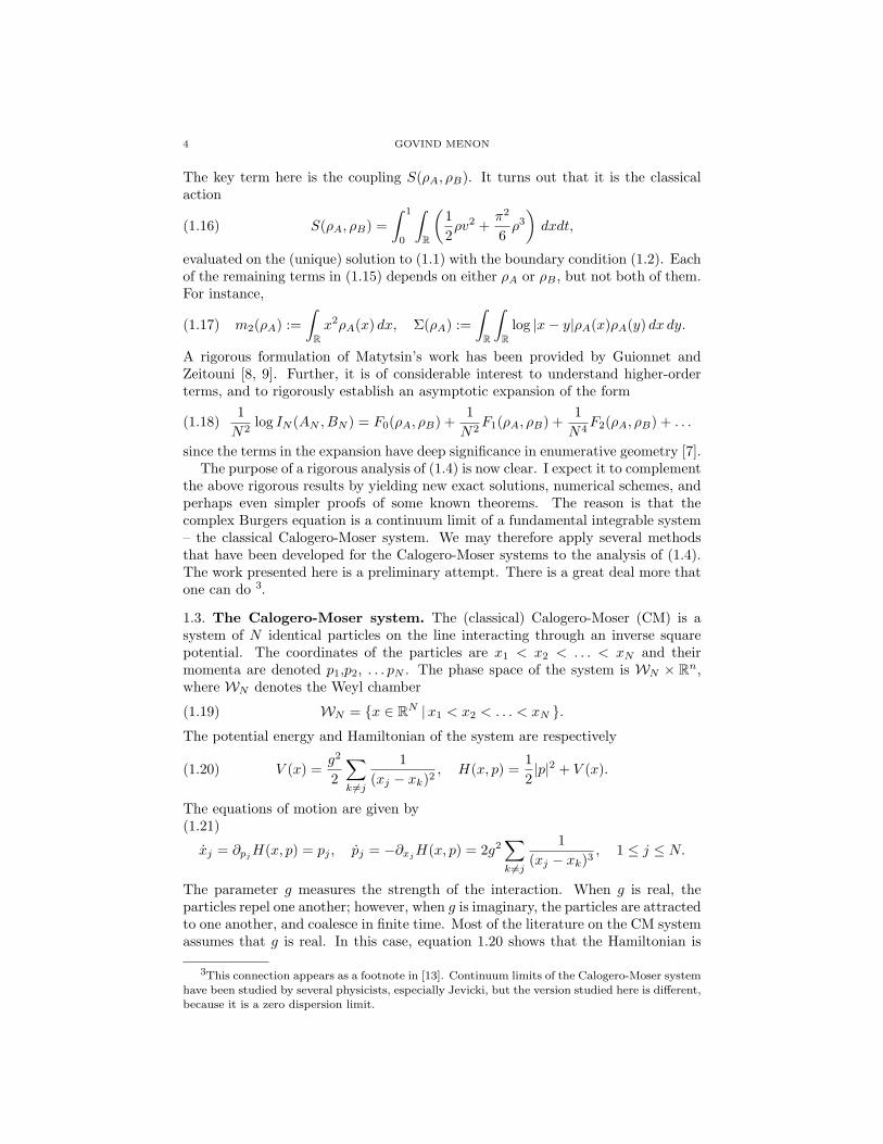
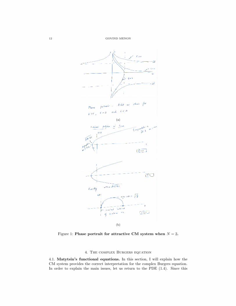
Before turning to the exact solvability of the CM system, let us build some intuitionby considering the simplest case, which is N = 2. Without loss of generality, wemay assume that the center of mass and mean momentum are 0. Therefore, usingequation (1.21) we find that s = x2 − x1 satisfies the second-order differentialequation

(1.23) s =4g2

s3.

This equation may be integrated using conservation of energy. We find that

(1.24) s2 = 2E − 2g2

s2, or s = ±

√2E − 2g2

s2.

The phase portraits for this system when g = 1 (repulsive) and g = i (attractive) areshown in Figure 1. When g = i, for each E < 0, there is a unique, positive solutionon a maximal interval (−T (E), T (E) with limt→±T (E) s(t) = 0. This solution has asquare-root singularity s(t) ∼ (T (E)−t)1/2 and s(t) ∼ (t+T (E))1/2 as t → ±T (E),since s ∼ ±s−1 as s → 0+. This critical solution is of interest to us for the followingreason. It gives rise to an exact solution to the boundary value problem (1.1)–(1.2).

1.4. An exact solution to complex Burgers. Bun, Bouchaud, Majumdar andPotters [5] 4 observed that (1.1)–(1.2) may be solved exactly by substituting theansatz

(1.25) f(x, t) = b(t)x + i

√4σ(t)2 − x2

2σ(t), |x| ≤ 2σ(t),

in equation (1.4), and solving the resulting ordinary differential equations for b(t)and σ(t). The exact form of this solution may be found in their work; what I wouldlike to point out here is that σ(t) and b(t) are related as follows:

(1.26) σ = − 4σ3

, b(t) =σ

σ.

That is, the N = 2 CM system is embedded within this exact solution, and b isobtained by the Riccati transformation of σ(t). The solution is symmetric aboutt = 1/2 and may be extended to a maximal time interval corresponding to thecritical solution to the CM system with N = 2. This calculation is reminescentof the construction of solitons and breathers via a pole ansatz, and I suspect thatseveral other exact solutions may be constructed in this manner.

4Matytsin makes a similar ansatz to solve induced QCD [13, Sec. 4].

6 GOVIND MENON

2. Large deviations for Dyson Brownian motion and the CM system

2.1. The principle of least action. The CM system arises naturally in the studyof the HCIZ integral through a somewhat unexpected confluence of two differentvariational problems. Recall that the equations of classical mechanics may be for-mulated using the principle of least action. The Lagrangian for the CM system isthe function

(2.1) L(x, y) =12|y|2 − V (x), x ∈ WN , y ∈ RN .

We consider C1 paths γ : [0, 1] →WN with boundary conditions γ(0) = (a1, a2, . . . , aN )and γ(1) = (b1, b2, . . . , bN ) and we associate to each path the action

(2.2) S[γ(·)] =∫ 1

0

L(γ(s), γ(s)) ds.

The principle of least action asserts that the ‘true’ path is a minimizer for the abovevariational principle. In this case, the Euler-Lagrange equations are precisely theequations of motion for the CM system (we’re using p = x). This is a formalprinciple and it is not always true that there is a minimizing path for the repulsiveCM system. Surprisingly, the attractive CM system is better behaved.

Lemma 2.1. Assume g = iκ for some κ ∈ R . Assume given any two pointsa and b in the Weyl chamber WN and any T > 0. Then there is a unique C1

path γ : [0, T ] → WN with γ(0) = a and γ(T ) = b that minimizes the action. Inparticular, for every a, b ∈ WN and T > 0, there exists a unique solution to theCM system defined on [0, T ] such that γ(0) = a and γ(T ) = b.

Sketch of the proof. The main point is that when g is imaginary, the LagrangianL(x, y) of the CM system is strictly convex in both x and y, since

(2.3) L(x, y) =12|y|2 +

κ2

2

∑k 6=j

1(xj − xk)2

, x ∈ WN , y ∈ RN .

Further, the Weyl chamber WN is a convex set, since it may be written as anintersection of half-spaces. A standard argument yields existence, uniqueness andsmoothness of minimizers.

2.2. Large deviations of Dyson Brownian motion. Let us now indicate howan a priori different variational principle is connected to this approach. The startingpoint for Guionnet and Zeitouni, as well as Bun et al , is the large deviations ofDyson Brownian motion. For each x ∈ WN we define the Coulomb energy

(2.4) U(x) =∑j<k

log |xj − xk|,

and recall that Dyson Brownian motion originating at a point a ∈ WN is the uniquesolution to the SDE

(2.5) dγl = −∂xlU(γ) dt + εdBl, γ(0) = a,

where dBl, l = 1, . . . , N are independent standard Brownian motions. Let us focuson Dyson Brownian bridges γ with γ(0) = a and γ(1) = b. Ignoring technicalities,as ε ↓ 0, such a bridge concentrates at the path that minimizes the Wiener action

(2.6) W [γ(·)] =12

∫ 1

0

|γ +∇U(γ)|2 ds,


where we again minimize over all C1 paths γ : [0, T ] → WN with γ(0) = a andγ(1) = b.

There is a lovely identity that connects the variational principle for the Wieneraction with the principle of least action for the CM system. Since U(x) is theCoulomb energy, we differentiate to find

(2.7) ∂xlU(x) =

∑j 6=l

1xl − xj

, l = 1, . . . , N.

Therefore, observing that the cross-terms cancel, we find

12|∇U(x)|2 =

12

N∑l=1

(∂xlU(x))2(2.8)

=12

N∑l=1

∑j 6=l

∑k 6=l

1(xl − xj)(xl − xk)

=12

∑k 6=j

1(xj − xk)2

=1g2

V (x),

where V (x) is the potential energy for the CM system defined in (1.20).We apply this identity to the Wiener action, to obtain

(2.9) W [γ(·)] =∫ 1

0

(12|γ|2 +

1g2

V (γ))

ds−∫ 1

0

γ · ∇U(γ) ds.

The last term is a total differential (a null Lagrangian in the terminology of thecalculus of variations), since

(2.10)∫ 1

0

γ · ∇U(γ) ds =∫ 1

0

d

dsU(γ(s)) ds = U(b)− U(a).

To summarize, we have obtained the following identity for the Wiener action

(2.11) W [γ(·)] =∫ 1

0

(12|γ|2 +

1g2

V (γ))

ds− (U(b)− U(a)) .

In particular, when g = i, the classical action S[γ()] and the Wiener action W [γ()]are minimized on the same path. Further, the minimum values are related by thedifference in the Coulomb energy

(2.12) argminW [γ(·)] = argminS[γ(·)]− (U(b)− U(a)) .

2.3. The Hamilton-Jacobi equation and Matytsin’s approach. Let us nowconnect the principle of least action to the Hamilon-Jacobi theory. FollowingArnol’d [3, §46C], we define the action function

(2.13) S(x, t) =∫ t

0

L(γ(s), γ(s)) ds,

where γ(t) is the extremal path connecting γ(0) = a to an arbitrary point x ∈ WN

at time t. Any initial condition would do, we have chosen γ(0) = a, only tobe concrete. By Lemma 2.1, the action function is well-defined when g is purelyimaginary. It then follows that S(x, t) solves the Hamilton-Jacobi equation

(2.14) ∂tS = H(x, ∂xS), i.e. ∂tS =12

N∑j=1

(∂xj S

)2 +g2

2

∑k 6=j

1(xj − xk)2

.

The reason for introducing this formalism here is to contrast Matytsin’s ap-proach to the HCIZ integral with Guionnet’s. Matytsin’s approach is not explicitly

8 GOVIND MENON

probabilistic. More precisely, he uses the heat equation in the space of Hermitianmatrices, but not Dyson Brownian motion. His starting point is the fact that atime-dependent version of the HCIZ integral solves a heat equation in WN . Hethen makes a WKB (or inverse Cole-Hopf) transformation to convert the linearheat equation to a nonlinear Hamilton-Jacobi equation, obtaining after some cal-culations a Hamilton-Jacobi equation with diffusion

(2.15) ∂tS =1

2N

N∑j=1

∂2xj

S +N

2

N∑j=1

(∂xj

S)2

− 12N3

∑k 6=j

1(xj − xk)2

.

At this stage, everything is exact. His key assumption is then to neglect the diffusionterm, obtaining the Hamilton-Jacobi equation [13, Eqn (2.7)]

(2.16) ∂tS =N

2

N∑j=1

(∂xj S

)2

− 12N3

∑k 6=j

1(xj − xk)2

.

We may write this equation in the form

(2.17) ∂tS = HN (x, S), HN (x, p) =N

2|p|2 − 1

2N3

∑k 6=j

1(xj − xk)2

,

Aside from scaling factors, equation (2.16) is identical to (2.14). Thus, implicit inMatytsin’s calculation is a reduction of the HCIZ integral to the CM system. (Thisrescaling is discussed in Section 5.)

The corresponding Lagrangian of the rescaled system is

(2.18) L(x, x) =1

2N

N∑j=1

x2j +

12N3

∑k 6=j

1(xj − xk)2

.

As explained in Section 5 when N →∞, the above Lagrangian has the the contin-uum limit

(2.19) L(ρ, v) =∫

Rρ(x, t)

(12|v(x, t)2 +

π2

3ρ3(x, t)

), dx,

Continuum limits of the CM system have been considered in the physics litera-ture [1, 17]. In these papers, N → ∞, but g does not depend on N . In ourwork, we must also take g → 0 at the rate 1/N . This changes the character of theproblem; we now have a zero-dispersion continuum limit, much like the celebratedLax-Levermore-Venakides theory.


3. Solving the Calogero-Moser system

There are many distinct solution techniques for the CM system. Two of these areconsidered here: (i) the projection method of Olshanetsky and Perelomov; and (ii)the use of pole dynamics and the doubled Benjamin-Ono equation (2BO). Thereis also a third approach that I have not worked out. This involves the use ofτ -functions and the KP hierarchy. I remark on this briefly at the end of this note.

In this section N is held fixed, and we drop the subscript N in the notation. Weassume given a, b ∈ WN and we write A = diag(a), B = diag(b). We set T = 1 andfocus on solving the boundary value problem for the CM system corresponding tothe principle of least action for paths γ : [0, 1] →WN with γ(0) = a, γ(1) = b. Thisis equivalent to determining the most likely path for the Dyson Brownian bridgeconnecting a and b as the noise vanishes when g is purely imaginary. In order toexplain the solution to this boundary value problem, it is important to first recallthe solution to the initial value problem for the CM system.

3.1. Moser’s matrices and the projection method. Consider the CM system

(3.1) xj = yj , yj = 2g2∑k 6=j

1(xj − xk)3

,

with the initial conditions x(0) = a ∈ WN , y(0) = v ∈ WN . Moser showed thatthis problem is completely integrable 5 by introducing the following matrices. Given(x, y), introduce the matrices P (x, y) and Q(x, y) with entries

Pjj = yj , Pjk =ig

(xj − xk), j 6= k,(3.2)

Qjj = −∑l 6=j

ig

(xj − xk)2, Qjk =

ig

(xj − xk)2.(3.3)

For comparison with continuum results with the Hilbert transform of the density,we also introduce the discrete matrix

(3.4) Hjj = 0, Hjk(x, y) =1

xj − xk, j 6= k.

While it requires considerable ingenuity to discover these matrices, a direct com-putation shows that (3.1) is equivalent to the Lax equation

(3.5) P = [P,Q].

As a consequence, the eigenvalues of P are constants of motion for (3.1). Thesecan be shown to be in involution and it follows that (3.1) is an integrable system.

Given a matrix H with real, distint eigenvalues, let eig(H) ∈ WN denote theeigenvalues listed in increasing order. We will use the following refinement ofMoser’s method introduced by Olshanetsky and Perelomov [15] to directly solvethe initial value problem for (3.1). Given (a, v) ∈ WN × RN , define the matrixP (a, v) as in (3.2). Then as long as the solution to (3.1) exists, it is given by thesimple formula

(3.6) x(t) = eig(A + tP (a, v)) .

There is an important difference between the repulsive case (g real) and the at-tractive case (g imaginary). When g is real, the matrix H(t) := A + tP (a, v) is

5He implicitly assumes g is real, but this is not necessary.

10 GOVIND MENON

Hermitian, the eigenvalues are real for all t, and the energy bound (1.22) ensuresthat the eigenvalues never collide. Thus, for each (a, v) ∈ WN × RN there is asolution to the CM system for every t ∈ R.

This is no longer true when g = i. The initial value problem is not defined forall time, and the eigenvalues collide. In fact, since A+ tP (a, v) is a real matrix thatis not symmetric, there is no a priori reason to expect that it has real eigenvalues(though this follows from (3.1), and remains true until the first collision of eigen-values). The above solution formula is called the projection method, since the CMflow is obtained by projecting the linear flow H(t) = A + tP (a, v) in Her(n) (wheng is real) or GL(n; R) (when g is imaginary) onto WN via the map H 7→ eig(H).

Nevertheless, Lemma 2.1 always allows us to solve the boundary value problem.More precisely, when g = i, given a, b ∈ WN , there is always a unique path withγ(0) = a and γ(1) = b that minimizes the action. This path is necessarily smooth,and in particular, if we set v = γ(0), we find that

(3.7) b = eig(A + P (a, v)).

Observe that b is given and v is determined implicitly through (3.7). This so-lution formula yields a shooting method to solve the boundary value problem.Thisyields the initial condition v for the CM flow connecting a to b. The entire flow isthen given by (3.6).

This solution formula allows us to approximate and visualize the transport mapfrom ρA to ρB that seems so mysterious when written in the form (1.1)–(1.2).Roughly, all we have to do is to approximate the spectral measures µA and µB

with N suitably chosen point masses, choose g = i/N , and find the CM solutionthat connects a and b. For instance, given ρA and ρB and N , let us define thevectors a, b ∈ WN by setting

(3.8) aj = µ−1A (

j

N), bj = µ−1

B (j

N), 1 ≤ j ≤ N,

where µA(x) :=∫ x

−∞ ρA(s) ds is the distribution function of µA, and we define theinverse as µ−1

A (α) = infxµA(x) ≥ α. We then apply the numerical scheme below.

3.2. A naive numerical scheme. In order to solve the discrete transport mapnumerically, it is only necessary to determine the initial velocity v that solves equa-tion (3.7). We use an eigenvalue solver and a Newton scheme as follows. Define thenonlinear map

(3.9) v 7→ λ(v) := eig(A + P (a, v)),

and consider the quadratic cost function

(3.10) h(v) =12|λ(v)− b|2.

The Newton-Raphson scheme to solve h(v) = 0 consists of an iterative sequencev(n) ∈ RN defined by

(3.11) v(n+1)j = v

(n)j − h(v(n))

∂vj h(v(n)), j = 1, . . . , N.

By the product rule, the gradient of h is

(3.12) ∂vj h(v) = (λ(v)− b) ·(∂vj λ(v)

)=

N∑k=1

(λk(v)− bk)(∂vj λk(v)

).


Therefore, our problem reduces to standard perturbation theory for eigenvalues.Let us recall the general facts, and then apply them in our context.

Consider a smooth curve (−1, 1) 3 τ 7→ C(τ) ∈ GL(N, R) in the space of ma-trices, such that eig(C(τ)) ∈ WN , τ ∈ (−1, 1). Let U(τ) denote the matrix ofeigenvectors and Λ(τ) = diag(eig(C(τ)) denote the diagonal matrix of eigenvalues.We differentiate the equation

(3.13) C(τ) = U(τ)Λ(τ)U−1(τ),

and rearrange terms to obtain

(3.14) U−1CU = [U−1U ,Λ] + Λ.

The diagonal entries of the commutator [U−1U ,Λ] vanish. Thus,

(3.15) Λ = diag(U−1CU

).

We apply the general formula(3.15) to our situation as follows. In order tocompute the derivative

(3.16) ∂vj λ(v)∣∣v=v(n)

we consider a curve C(τ) with

(3.17) C(τ) = A + igH(a) + ig diag(v(τ)), v(τ) = v(n) + τej

where ej ∈ Rn is the j-th standard basic vector. In this case,(3.18)

C(0) = A + igH(a) + ig diag(v(n)) = A + P (a, v(n)), and C(0) = diag (ej).

We then have

(3.19) ∂vjλ(v)

∣∣v=v(n) = ig diag

(U−1 diag(ej)U

),

where U = U(v(n)) is the matrix of eigenvectors of A + P (a, v(n)).In summary, the numerical scheme is as follows. Given v(n), we compute the

eigenvalues λ(n) and eigenvector matrix U (n) of A + P (a, v(n)) using an eigenvaluesolver for non-symmetric matrices. We then compute the cost function h(v(n))and its derivative using the formulas (3.10), (3.12) and (3.19). These yield thenext iterate v(n+1) in the Newton-Rapshon scheme. The scheme requires a carefulchoice of initial conditions. 6 In particular, since the matrix A + P (a, v(n)) is not-symmetric, we must stop the iteration if it has complex eigenvalues.

6As of Feb. 2016, I have not been able to use this scheme to solve the BVP! It appears thatwhat one needs is a multiple shooting method.

12 GOVIND MENON

(a)

(b)

Figure 1: Phase portrait for attractive CM system when N = 2.

4. The complex Burgers equation

4.1. Matytsin’s functional equations. In this section, I will explain how theCM system provides the correct interpretation for the complex Burgers equation.In order to explain the main issues, let us return to the PDE (1.4). Since this


equation is elliptic at all points where ρ(x, t) > 0, we cannot use the solutionformula (1.5) without assuming that f0 is analytic in a complex neighborhood ofthe x-axis. However, f0 cannot be analytic for any ρA with compact support, noteven for the exact solution (1.25)!

Matytsin does not let such mathematical niceties stop him, and he solves inducedQCD by the method of characteristics as follows. Let f0 and f1 denote f(x, 0) andf(x, 1) respectively. Define the forward characteristic map G+ : x 7→ x + f0(x) andthe backward characteristic map G− : x 7→ x − f1(x), and (formally) use (1.4) toobtain the identities

(4.1) G−(G+(x)) = x, G+(G−(x)), x ∈ R,

Matytstin formally solves these functional equations with boundary conditions

(4.2) Im(G+(x)) = πρA(x), Im(G−(x)) = πρB(x), x ∈ R,

by making a clever ansatz.In my view, the use of this functional equations does not actually shed any

light on the problem, since it is an easy consequence of the (unjustified) use of themethod of characteristics. Further, when one applies this method to the study ofthe Kosterlitz-Thouless phase transitions as in [14], the functional equation leadsto a problem with small divisors, a sure sign that there is something rather subtlein the background. Therefore, it strikes me as important to nail down the methodof characteristics in this problem. In particular, this requires a more careful speci-fication of the domain of the problem (Is x real or complex? How is f0 defined inthe complex plane, when we only prescribe ρA and ρB on the line? etc.).

4.2. The Hilbert and Cauchy transforms. Given a complex function u(x),x ∈ R, its Hilbert transform is defined by

(4.3) Hu(x) =p.v.

π

∫R

1λ− x

u(λ) dλ = x ∈ R

The principal value integral is defined by

(4.4) Hu(x) =p.v.

π

∫R

u(x− s)s

ds =1π

limε→0

∫|s|>ε

u(x− s)s

ds.

The Hilbert transform is a bounded operator on Lp(R), 1 < p < ∞. When theFourier transform of u is defined by

(4.5) u(ξ) =∫

Re−2πixξu(x) dx,

the Hilbert transform has the multiplier 7

(4.6) (Hu)(ξ) = −isgn(ξ) u(ξ), ξ ∈ R.

When u is real, the Hilbert transform provides the boundary values of the com-plementary harmonic function for the harmonic extension of u. Here is what thismeans. Assume u is real and consider its Cauchy transform

(4.7) Cu(z) =∫

R

1λ− z

u(λ) dλ, z ∈ C\R.

7We use Stein’s convention to define the Hilbert transform, but the modern sign conventionfor the Fourier transform. This is why the multiplier is −i sgn(ξ), as compared with i sgn(ξ) [16,p.55].

14 GOVIND MENON

The function Cu is analytic in C\R. When u is a positive density it is a Herglotzfunction.8 Let (Cu)±(x) denote its boundary values as z → x ∈ R from the upperand lower-half plane respectively. Then

(4.8) Cu±(x) = πHu(x)± iπu(x), x ∈ R.

4.3. Free convolution with the semicircle law. To build some intuition forcomplex Burgers equation, let us first recall the following fact from free probabilitytheory. Let νt denote the semicircle law with width 2t

(4.9) dνt(x) =1

2πt

√4t− x2, |x| ≤ 2t.

Assume given a measure µA with density ρA, and let µt = µA νt denote the freeconvolution of µA with the semicircle law νt. Let ρt denote the density of µt and(abusing notation) let us set f(z, t) = Cµt(z) = Cρt(z). Then a basic fact in freeprobability theory is that f solves the complex Burgers equation

(4.10) ∂tf − f∂zf = 0, t > 0, z ∈ C+.

The difference with (1.4) is that we are not explicit about the domain of our func-tion, and the use of complex characteristics is completely justified. The character-istics of (4.10) solve the ordinary differential equation

(4.11) z = −f(z, t), z ∈ C+.

On the real axis, these ordinary differential equations become

(4.12) x = πHρt(x), y = −πρt(x), x ∈ R, t > 0.

Since ρt ≥ 0, the characteristics always flow out of C+. Thus, the domain C+

is positively invariant under the flow (4.11). This property is what allows us touse the method of characteristics in this problem. In summary, in the absence of aboundary condition at t = 1, equation (1.4) is well-posed on the domain C+×(0,∞)by extending ρ(·, t) to the analytic function f(z, t) using the Cauchy transform. Itmay also be checked that for each t > 0 the PDE continues to hold on the x-axis.With a little work, one can now establish regularity for ρt (Biane does not explicitlyuse the method of characteristics, but it is implicit in his proof[4]).

The complex Burgers equation (4.10) should be thought of as the analogue of theheat equation in free probability. The solution admits the following direct stochasticinterpretation. Let St denote a standard free Brownian motion, and let A be anoperator with spectral measure ρA that is free with respect to the process St. Thenρt is the spectrum of A + St. The appearance of complex Burgers equation in

8There is a rather annoying difference in sign conventions between the use of Cauchy transformsin the theory of Herglotz function and in free probability theory. Herglotz functions are analyticfunction f : C+ → C+. A classical representation theorem asserts that each Herglotz functionis the potential of a positive measure, that is f = Cµ where µ is a positive measure on R. Thissign convention ensures that Herglotz functions are closed under composition and that they arematrix monotone [6]. In the literature on free probability, the Cauchy transform is normalized asGµ(z) := −Cµ(z). The transform Gµ is an anti-Herglotz function, that is Gµ : C+ → C−. Thisconvention has the unfortunate effect of flipping the sign in the inversion formula. For simplicity,assume µ has a density ρ. Then

limy↓0

Re Gµ(x + iy) = πHρ(x), limy↓0

Im Gµ(x + iy = −πρ(x),

in comparison with (4.8). Since Matytsin’s starting point is the function f = v+ iπρ, we have pre-ferred to use the convention on Herglotz functions, rather than the convention of free probability.


Matytsin’s work also has a free probability interpretation. However, now we mustconsider a free Brownian bridge, not a free Brownian motion. Let S be a standardsemicircular operator, and let A and B be operators with spectral measures ρA

and ρB respectively, and suppose A,B and S are free with respect to one another.Then the density ρ(·, t) corresponding to the solution to (1.4) is the law of the freevariable 9

(4.13) Xt = (1− t)A + tB +√

t(1− t) S, t ∈ [0, 1].

4.4. The domain for (1.4). In order to solve (1.4) by the method of character-istics, we must extend the spatial domain from x in the support of ρ, to a suitablesubset of the complex plane. Classical potential theory and the calculation abovesuggests that the natural extension of ρ to the complex plane is provided by itsCauchy transform. Further, the calculations above show that each positive densityρ induces a velocity field πH(ρ)(x). However, when solving the boundary valueproblem (1.2)–(1.4), it is clear that the ‘shooting velocity’ from ρA cannot simplybe πH(ρA), since this would imply ρt = ρA νt. Thus, we are finally led to sepa-rate the velocity field into two parts: a self evolution corresponding to the Hilberttransform and free convolution, and a second part, which ‘shoots’ ρA at t = 0 toρB at t = 1. 10

This idea is implemented as follows. For each δ > 0 we define the open stripSδ = z || Im(z)| < δ . Given ρA and ρB we seek δ > 0 and a function f = f+ + f−such that f− is analytic in Sδ and

(4.14) f+(z, t) = Cρ(·, t), z ∈ C\R.

Observe that this separates the velocity field v(x, t), x ∈ R into two parts:

(4.15) v+(x, t) = πH(ρ(·, t))(x) = Re f+(x, t), v−(x, t) = Re f−(x, t), x ∈ R.

The first part corresponds to the ‘self-velocity’ of free convolution. The secondpart is the ‘driving’ velocity that steers ρ(·, t) from ρA to ρB . The point is that thesolution formula (1.5) may be rigorously applied for z ∈ Sδ.

The difference between the velocity v(x, t) and Hρ(·, t) may be computed for theexact solution (1.25) constructed in [5]. In this example, we find that

(4.16) f−(z, t) =(

b(t) +1

2σ2(t)

)z.

In this case, Sδ = C and f−(z, t) is an entire function of z. Matytsin always assumesthat the ‘driving’ velocity field is a polynomial, which is what allows him to use themethod of characteristics. However, this situation is atypical, and for many otherinteresting solutions, f− is analytic only in a strip of finite width.

4.5. A generalized Hilbert transform. Aficionados of integrable systems areaware of many unexpected connections between distinct models. For instance, ithas been known since the work of Airault, McKean and Moser that the CM systemdescribes the evolution of rational solutions to the KdV hierarchy [2]. Roughly, thepoles of certain rational solutions to KdV evolve according to the CM system. Suchconnections were treated systematically for the KP hierarchy by Krichever [12]. The

9This statement follows Guionnet [8]. But surely one should be able to use a ‘true’ freeBrownian bridge (i.e. a process St), rather than just scaling a fixed free variable S.

10In the discrete CM system, this splitting correspond to the off-diagonal and diagonal termsof the matrix P defined in (3.2).

16 GOVIND MENON

version of this set of ideas that is most useful for us is a connection between CMsolutions and the doubled Benjamin-Ono equation studied by Abanov, Bettelheimand Wiegmann [1] (see also [17]).

In order to introduce these equations, we will modify the definition of the Hilberttransform as follows. Consider a simple closed curve Γ that separates the complexplane into exterior and interior domains, denoted Ω± respectively. Given a suffi-ciently regular function ϕ : Γ → C we extend it to the analytic functions

(4.17) ϕ±(z) =1

2πi

∮Γ

ϕ(s)s− z

ds, z ∈ Ω±.

The Plemelj formulas provide jump and continuity conditions on the curve z ∈ Γ

(4.18) ϕ−(z)− ϕ+(z) = ϕ(z), ϕ−(z) + ϕ+(z) =p.v.

πi

∮Γ

ϕ(s)s− z

ds.

Therefore, we may define the Hilbert transform with respect to Γ, as

(4.19) HΓϕ(z) =p.v.

π

∮Γ

ϕ(s)s− z

ds = i (ϕ−(z) + ϕ+(z)) .

Of particular importance for us are the following eigenfunctions of the operator HΓ.Using the above formulas, we find that when

(4.20) ϕ(z) =1

z − a, a ∈ Ω+ ∪ Ω−,

(4.21) HΓϕ(z) = −iϕ(z), a ∈ Ω+, HΓϕ(z) = +iϕ(z), a ∈ Ω−.

These eigenfunctions are computed as follows. To be concrete, we assume a ∈ Ω+.Then ϕ(z) is analytic in a sufficiently small neighborhood of Γ, and the integrandin (4.17) may be written as follows:

(4.22)ϕ(s)s− z

=1

z − a

(1

s− a− 1

s− z

).

Substituting in (4.17), we find that

(4.23) ϕ−(z) =−1

z − a, ϕ+(z) = 0.

Similarly, when a ∈ Ω− we find

(4.24) ϕ−(z) = 0, ϕ+(z) =1

z − a.

We substitute (4.23)–(4.24) in (4.19) to obtain (4.21).

4.6. The doubled Benjamin-Ono equation. The Benjamin-Ono equation withrespect to the curve Γ is the PDE

(4.25) ∂tf + f∂zf =g

2∂2

zHΓf, z ∈ Γ, t > 0.

This PDE is connected to the CM system via the following ansatz. Assume Γ is asufficiently curve that circles a sufficiently large interval I on the x-axis. AssumeN and M are integers, and let x1(t) < x2 < . . . < xN (t) be points on I, and letwk(t)M

k=1 be points in Ω+ ⊂ C. We substitute the ansatz

(4.26) f(z, t) =N∑

j=1

ig

z − xj(t)−

M∑k=1

ig

z − wk(t),


into (4.25), use (4.20)–(4.21), and the identity

(4.27)1

z − α

1(z − β)2

+1

(z − α)21

z − β=

1α− β

(1

(z − α)2− 1

(z − β)2

),

to obtain the ordinary differential equations

xj =N∑

l=1,l 6=j

ig

xl − xj−

M∑m=1

ig

wm − xj, j = 1, . . . , N,(4.28)

wk = −N∑

l=1

ig

wk − xl+

M∑m=1,m 6=k

ig

wk − wm, k = 1, . . . ,M.(4.29)

Thus, we obtain a closed system of N +M equations for the evolution of the poles.Now it turns out that one may further differentiate these equations, and use (4.28)and (4.29) to eliminate xj and wk to find that

(4.30) xj =∑l 6=j

2g2

(xj − xl)3, j = 1, . . . , N.

Thus, the poles xj satisfy the CM system (1.21). In order to ensure that thesesolutions stay real, we must ensure that the initial w’s are such that xj(0) is realfor each j. Equation (4.28) shows that this always holds provided M is even andthe poles w are pairs of complex conjugates. The w’s satisfy a complementary CMsystem. Except for the coupling through the initial condition, these two systemsevolve independently (despite what (4.28)–(4.29) suggests at first sight).

4.7. τ functions and the zero dispersion continuum limit. Though the de-tails are not presented here, it is a short step from (ii) to the use of τ -functionsto construct multi-soliton solutions to (1.1). Roughly, exact solutions to the CMsystem may be expressed as determinants using τ -functions for the KP hierarchy.Further, the N →∞, g = O(1) continuum limit of these solutions has already beenworked out by Abanov et al . However, it does remain to see how this approachyields solutions to the complex Burgers equation when we also take g → 0. If werecall that the zero-dispersion limit of (real valued) KdV is Burgers equation – thisis the core observation of Lax and Levermore – we see exactly how the N → ∞limit studied by Matytsin is an analogous zero-dispersion limit. In order to explainthis point, let us examine the scaling limit more carefully.

18 GOVIND MENON

5. The scaling limit

Our starting point is the Calogero-Moser system with the rescaled Hamiltonian

(5.1) H(x, p) =N

2|p|2 − κ2

2N3

∑k 6=j

1(xj − xk)2

.

In the notation of equation (1.20), we have chosen

(5.2) g =iκ

N,

where κ is a fixed parameter, independent of N . In most of what follows κ = 1.This parameter is included to provide a unified treatment of the attractive andrepulsive CM system.

Recall that fluid equations such as (1.1) may be written in either the Eulerian orLagrangian formulation. We first write the equations of motion for the particle sys-tem with Hamiltonian (5.1) in a way that is suggestive of the continuum limit in theLagrangian formulation. To this end, let α ∈ [0, 1] denote the material coordinate;the position of the particle x(α, t) is given implicitly through the relationship

(5.3)∫ x(α,t)

−∞ρ(s, t) ds = α,

and the map α 7→ x(α, t) is an increasing function. At points where ρ(x, t) > 0, wemay differentiate (5.3) to obtain the relationship

(5.4) x′(α, t) := ∂αx(α, t) =1

ρ(x, t).

The Lagrangian form of equation (1.1) is the system

∂tx(α, t) = u(α, t),(5.5)

∂tu(α, t) = −κ2π2 x′′

(x′)4,(5.6)

where the Eulerian and Lagrangian velocity fields are related via

(5.7) u(α, t) = v(x(α, t), t) = v(x, t).

The equivalence between the two systems of equations at points where ρ(x, t) isstrictly positive and differentiable may be established by differentiating (5.5) andusing (5.3), (5.4) and (5.7).

We now explain how to obtain (5.5) as the N →∞ limit of the CM system withHamiltonian (5.1). For each N , let us denote the vector x ∈ RN (resp. v, p), asa function x(N)(α, t) defined at each lattice point αk = k/N , 1 ≤ k ≤ N by therelation

(5.8) x(N)(αk, t) = xk(t), p(N)(αk, t) = pk(t), u(N)(αk, t) = uk(t).

In these variables the equations of motion for the Hamiltonian (5.1) take the form

∂tx(N)(α, t) = Np(N)(α, t),(5.9)

∂tp(N)(α, t) =

2κ2

N3

∑β 6=α

1(x(N)(β, t)− x(N)(α, t)

)3 ,(5.10)


where the Lagrangian coordinates α and β range over the index set k/N , 1 ≤ k ≤ N .In the limit, we expect the particle velocities to be well-defined, and working withv(N) instead of p(N), we find

∂tx(N)(α, t) = u(N)(α, t),(5.11)

∂tu(N)(α, t) =

2κ2

N2

∑β 6=α

1(x(N)(β, t)− x(N)(α, t)

)3 .(5.12)

It is easy to see how (5.11) converges to (5.5), when we scale the momentum asin (5.1). Indeed, with this scaling, the kinetic energy in the Hamiltonian is

(5.13)N

2

N∑k=1

p2k =

12N

N∑k=1

u2k =

12N

N∑k=1

∣∣∣u(n)(αk, t)∣∣∣2 ≈ 1

2

∫ 1

0

|u(α, t)|2 dα,

using the Riemann sum to approximate the integral under the assumption that

(5.14) u(n)(αk, t) ≈ u(αk, t), 1 ≤ k ≤ N.

However, it is necessary to treat the singular terms systematically in order toobtain the continuum limit (5.6) from (5.12) under the scaling (5.2). We will explaina general procedure to approximate such singular sums.

5.1. Approximations with the Euler-MacLaurin formula. Assume f : [0, 1] →R is a C∞ function. The Euler-MacLaurin formula∫ 1

0

f(α) dα =1N

(12f(0) +

N1∑k=1

f(k

N) +

12f(1)

)(5.15)

+1

12N2(f ′(0)− f ′(1))− 1

720N4(f ′′′(0)− f ′′′(1)) + . . .

provides an asymptotic expansion for the Riemann integral of f . Observe that theerror terms are controlled by the derivatives of f at the endpoints 0 and 1.

Our interest lies in the leading order asymptotics of sums of the form

(5.16)N∑

k=1,k 6=j

1(xk − xj)p

,

when j = Nα where α ∈ (0, 1) is held fixed, and p is an integer (p = 1, 2 and 3). Inorder to apply the Euler-MacLaurin formula to such functions, we will replace thesummand with a suitably regularized function fp, (p = 1, 2 and 3) that regularizesthe singularity near k = j. In what follows, we fix α, set j = αN , and we usek = βN to denote the indices being summed over.

5.1.1. Case 1. p = 1 . Fix ε > 0 and consider separately the sum over β such that|α−β| ≥ ε and |α−β| < ε. In the region |α−β| ≥ ε, the summand is non-singularand we find

(5.17) limN→∞

1N

∑|j−k|<εN

1xk − xj

=∫|α−β|>ε

1x(β)− x(α)

dβ.

In order to treat the singular region, we consider the function

(5.18) f1(s) =1

x(α + s)− x(α)− 1

x′(α)s, |s| < ε.

20 GOVIND MENON

Under the assumption that x(β) is C2 at β = α, we find that

(5.19) lims→0

f1(s) =12

x′′(α)x′(α)

.

We apply the Euler-MacLaurin approximation to f1 on the interval |s| < ε to obtain

(5.20)1N

∑|l|<εN

(1

x(α + l/N)− x(α)− N

x′(α)l

)=∫|α−β|<ε

f1(β) dβ + O(1N

).

On the other hand, we also have

(5.21)∑

|l|<εN, l 6=0

1x′(α)l

= 0.

Therefore, we can remove this term from the summand. Further, we can alsoremove the regularizing term in the integrand, provided we replace the divergentintegral with its principal value. Combining these steps, we find that

(5.22) limN→∞

∑|l|<εN

1x(α + l/N)− x(α)

= p.v.

∫|α−β|<ε

1x(β)− x(α)

dβ.

5.1.2. Case 2. p = 2 . As in Case 1, it is only necessary to consider the sum inthe range |β − α| < ε for some fixed ε > 0. The regularizing function in this casetakes the form

(5.23) f2(s) =1

(x(α + s)− x(α))2− c0 + c1s

s2, |s| < ε,

where the coefficients c0 and c1 are determined by the condition that f2(s) is con-tinuous at s = 0. We find after some algebra (as explained below for the case p = 3)that

(5.24) f2(s) =1

(x(α + s)− x(α))2− 1

(x′(α)2s2+

x′′(α)x′(α)s

, |s| < ε,

Thus, adding the regularizing terms, and using the fact that∑|j−k|<ε,j 6=k(k −

j)−1 = 0 and∑∞

l=1 l−2 = ζ(2) = π2/6, we obtain the approximation

1N

∑|j−k|<εN,j 6=k

1(xk − xj)2

=Nπ2

3x′(α)2

+1N

∑|j−k|<εN,j 6=k

1(xk − xj)2

− N2

(x′(α)2(j − k)2+

Nx′′(α)x′(α)(j − k)

+ O(1N

).

By the Euler-MacLaurin expansion, the second term on the right hand side is O(1),since it converges to the integral

∫|s|<ε

f2(s) ds. Thus,

(5.25) limN→∞

1N2

∑|j−k|≤εN,j 6=k

1(xk − xj)2

=π2

3x′(α)2.

This also shows that the discrete CM potential energy has the scaling limit

(5.26) limN→∞

−κ2

N3

∑k 6=j

1(xk − xj)2

= −κ2

∫ 1

0

π2

3x′(α)2dα.


The above convergence of the potential energy is enough to deduce that (5.6) is thecontinuum limit of the CM system, but let us also show that the same techniqueyields the convergence of (5.12) to (5.6).

5.1.3. Case 3. p = 3 . Observe that in Case 2, the leading order term is local (i.e.not a singular integral, unlike Case 1). This is typical for all p ≥ 2. When p = 3,we proceed as for p = 2, seeking a function

(5.27) f3(s) =1

(x(α + s)− x(α))3− c0 + c1s + c2s

2

s3,

that is continuous as s → 0. Assuming that we have found such an expansion, wefix an ε > 0, use the fact that

(5.28) 0 =∑

|j−k|<εN,j 6=k

1(j − k)3

=∑

|j−k|<εN,j 6=k

1(j − k)

and apply the Euler-MacLaurin expansion to f3 in the interval (α − ε, α + ε), toobtain the asymptotic expansion

(5.29)1

N2

∑ 1(xk − xj)

3 = c1

∑ 1(j − k)2

+1

N2

∑f3(xk − xj),

where the sum is over the index k in the range |k − j| < ε, k 6= j.The coefficients c0, c1 and c2 are computed as follows. For brevity, let us denote

the Taylor expansion

(5.30) x(α + s)− x(α) = a1s + a2s2 + a3s

3 + . . .

The continuity of f3 at s = 0 imposes the requirement that

(5.31) s3 − (a1s + a2s2 + a3s

3)3(c0 + c1s + c2s

2)

= O(s6),

which yields the following set of polynomial equations for c0, c1 and c2 in terms ofa1, a2 and a3:

O(1) : c0a31 = 1,

O(s) : c1a31 + 3c0a

21a2 = 0,

O(s2) : a31c2 + 3c1a

21a2 + 3c0

(a1a

22 + a2

1a3

)= 0,

These equations have a unique solution when a1 6= 0. We find that

(5.32) c0 =1a31

, c1 = −3a2

a41

, c2 = 6a22

a51

− 3a3

a41

.

Equations (5.29) tells us that we only need c1. Thus, using the fact that a1 anda2 are the first two terms in the Taylor expansion of x(α + s)− x(α), we use (5.29)and (5.32) to find that for every ε > 0,

(5.33) limN→∞

1N2

∑|j−k|<ε,j 6=k

1(xk − xj)3

= −π2

332

x′′(α)x′(α)4

= −π2

2x′′(α)x′(α)4

.

We apply (5.33) to (5.12) to obtain equation (5.6), the continuum CM system inLagrangian coordinates.

22 GOVIND MENON

6. The Lax pair for the continuum limit

We have now found two distinct descriptions of the continuum limit of the CMsystem. The Eulerian formulation (1.1), and the Lagrangian formulation (5.5) and(5.6). It is easy to guess the form of the Lax pair for the Lagrangian formulationusing the formulas (3.2)–(3.3), though these must be written in weak form.

Let h : [0, 1] → C be a test function that vanishes at all points where x′(α) = 0,and define the singular integral operators

Ph(α) = u(α)h(α) + κ p.v.

∫ 1

0

h(β)x(β)− x(α)

dβ(6.1)

Qh(α) = −κ p.v.

∫ 1

0

h(β)− h(α)(x(β)− x(α))2

dβ.(6.2)

These operators are formal limits of the Lax pair (3.2)–(3.3), when g = iκ/N . Thecondition that the test function h vanishes at all points where x′(α) = 0 is necessaryto ensure that the integrals are meaningful. This condition is cumbersome and itis simpler to work with the operators written in Eulerian coordinates.

Let ϕ : R → R be a smooth test function and recall that ρ(x, t) and v(x, t) arethe Eulerian density and velocity field for (1.1). We define the operators

Lϕ(x) = v(x, t)ϕ(x) + κ p.v.

∫R

f(s)s− x

ρ(s, t) ds,(6.3)

Mϕ(x) = −κ p.v.

∫R

f(s)− f(x)(s− x)2

ρ(s, t) ds.(6.4)

We claim that when κ = 1, (1.1) and (1.4) is equivalent to the Lax equation

(6.5) L = [L,M ].

While we have been led to this Lax pair by taking the continuum limit of theN particle CM system, it may be used directly for the analysis of (1.1). Theverification that (6.5) is equivalent to (1.1) requires a careful computation, at theheart of which is the following commutator identity for the Hilbert transform. Aswith many Fourier identities, it is enough to check the lemma on functions inthe Schwartz class S(R), and then to use standard density arguments to extendthe identity to general function classes, say Lp(R). Given a Schwartz functionn ∈ S(R), we define the multiplication operator Mn : S → S by h 7→ Mnh,Mnh(x) = n(x)h(x).

Lemma 6.1. Suppose p ∈ S(R). Then we have the following commutator identity

(6.6) [H,MHp] = Mp +HMpH.

The precise domain of definition of the above operators takes some care, sincethe Hilbert transform does not map S(R) into itself, but I’m going to ignore thesetechnicalities for now. The main point is really that the above lemma provides theright way to think about the cancellation (4.28), which underlies the equivalencebetween the Lax equation (3.5) and the discrete CM system (3.1).

Proof. The lemma is best proved with Fourier multipliers. Let ϕ ∈ S(R) andconsider

[H,MHp]ϕ = HMnϕ−MnHϕ.


Since H has multiplier −isgn(ξ) and Mnϕ = n ? ϕ, we find that

(6.7) HMHpϕ = −isgn(ξ)(Hp ? ϕ

)(ξ) = −sgn(ξ)

∫R

sgn(η)p(η)ϕ(ξ − η) dη.

A similar computation reveals that

(6.8) MHpHϕ = −∫

Rsgn(η)sgn(ξ − η)p(η)ϕ(ξ − η) dη.

Thus, we have found that the Fourier transform of [H,MHp]ϕ is

(6.9)∫

Rsgn(η) (sgn(ξ − η)− sgn(ξ)) p(η)ϕ(ξ − η) dη.

Now an elementary computation shows that

(6.10) sgn(η) (sgn(ξ − η)− sgn(ξ)) = 1− sgn(η)sgn(ξ − η), ξ, η ∈ R.

Therefore, the Fourier transform of [H,MHp]ϕ is

(6.11)∫

Rp(η)ϕ(ξ − η) dη −

∫R

sgn(η)sgn(ξ − η)p(η)ϕ(ξ − η) dη,

which is the Fourier transform of (Mp +HMpH)ϕ.

References

[1] A. G. Abanov, E. Bettelheim, and P. Wiegmann, Integrable hydrodynamics of Calogero-Sutherland model: bidirectional Benjamin-Ono equation, J. Phys. A, 42 (2009), pp. 135201,24.

[2] H. Airault, H. P. McKean, and J. Moser, Rational and elliptic solutions of the Korteweg-de Vries equation and a related many-body problem, Comm. Pure Appl. Math., 30 (1977),pp. 95–148.

[3] V. I. Arnol′d, Mathematical methods of classical mechanics, Springer-Verlag, New York-Heidelberg, 1978. Translated from the Russian by K. Vogtmann and A. Weinstein, GraduateTexts in Mathematics, 60.

[4] P. Biane, On the free convolution with a semi-circular distribution, Indiana Univ. Math. J.,46 (1997), pp. 705–718.

[5] J. Bun, J.-P. Bouchaud, S. N. Majumdar, and M. Potters, Instanton approach to largen harish-chandra-itzykson-zuber integrals, Physical review letters, 113 (2014), p. 070201.

[6] W. F. Donoghue, Jr., Monotone matrix functions and analytic continuation, Springer-Verlag, New York-Heidelberg, 1974. Die Grundlehren der mathematischen Wissenschaften,Band 207.

[7] I. P. Goulden, M. Guay-Paquet, and J. Novak, Monotone Hurwitz numbers and the HCIZintegral, Ann. Math. Blaise Pascal, 21 (2014), pp. 71–89.

[8] A. Guionnet, First order asymptotics of matrix integrals; a rigorous approach towards theunderstanding of matrix models, Comm. Math. Phys., 244 (2004), pp. 527–569.

[9] A. Guionnet and O. Zeitouni, Large deviations asymptotics for spherical integrals, J. Funct.Anal., 188 (2002), pp. 461–515.

[10] Harish-Chandra, Differential operators on a semisimple lie algebra, American Journal ofMathematics, 79 (1957), pp. 87–120.

[11] C. Itzykson and J.-B. Zuber, The planar approximation. ii, Journal of MathematicalPhysics, 21 (1980), pp. 411–421.

[12] I. M. Krichever, Rational solutions of the Kadomcev-Petviasvili equation and the integrablesystems of N particles on a line, Funkcional. Anal. i Prilozen., 12 (1978), pp. 76–78.

[13] A. Matytsin, On the large-N limit of the Itzykson-Zuber integral, Nuclear Phys. B, 411(1994), pp. 805–820.

[14] A. Matytsin and P. Zaugg, Kosterlitz-Thouless phase transitions on discretized randomsurfaces, Nuclear Phys. B, 497 (1997), pp. 658–698.

24 GOVIND MENON

[15] M. A. Ol′shanetskiı, A. M. Perelomov, A. G. Reı man, and M. A. Semenov-Tyan-Shanskiı, Integrable systems. II, in Current problems in mathematics. Fundamental direc-tions, Vol. 16 (Russian), Itogi Nauki i Tekhniki, Akad. Nauk SSSR, Vsesoyuz. Inst. Nauchn.i Tekhn. Inform., Moscow, 1987, pp. 86–226, 307.

[16] E. M. Stein, Singular integrals and differentiability properties of functions, Princeton Math-ematical Series, No. 30, Princeton University Press, Princeton, N.J., 1970.

[17] M. Stone, I. Anduaga, and L. Xing, The classical hydrodynamics of the calogero–sutherlandmodel, Journal of Physics A: Mathematical and Theoretical, 41 (2008), p. 275401.

[18] J.-B. Zuber, Introduction to random matrices. Lectures at Les Houches (May 2011) andBangalore (Jan 2012), 2012.

Division of Applied Mathematics, Box F, Brown University, Providence, RI 02912.E-mail address: govind [email protected]

the complex burgers equation, the hciz integral … · the complex burgers equation, the hciz...

Documents