the composite absolute penalties family for grouped …

Submitted to the Annals of Statistics

THE COMPOSITE ABSOLUTE PENALTIES FAMILY FOR

GROUPED AND HIERARCHICAL VARIABLE SELECTION

By Peng Zhao and Guilherme Rocha and Bin Yu†

University of California at Berkeley

Extracting useful information from high-dimensional data is an

important focus of today’s statistical research and practice. Penal-

ized loss function minimization has been shown to be effective for

this task both theoretically and empirically. With the virtues of both

regularization and sparsity, the L1-penalized squared error minimiza-

tion method Lasso has been popular in regression models and beyond.

In this paper, we combine different norms including L1 to form

an intelligent penalty in order to add side information to the fitting

of a regression or classification model to obtain reasonable estimates.

Specifically, we introduce the Composite Absolute Penalties (CAP)

family which allows given grouping and hierarchical relationships be-

tween the predictors to be expressed. CAP penalties are built by

defining groups and combining the properties of norm penalties at

the across group and within group levels. Grouped selection occurs

for non-overlapping groups. Hierarchical variable selection is reached

∗ The authors would like to gratefully acknowledge the comments by Nate Coehlo,

Jing Lei, Nicolai Meinshausen, David Purdy and Vince Vu, the partial support from NSF

grants DMS-0605165, DMS-03036508, DMS-0426227, ARO grant W911NF-05-1-0104, and

NSFC grant 60628102 and comments from the referees.† Bin Yu gratefully acknowledges the support from a Miller Research Professorship in

Spring 2004 from the Miller Institute at UC Berkeley and a Guggenheim Fellowship in

2006.

AMS 2000 subject classifications: Primary 62J07

Keywords and phrases: linear regression, penalized regression, variable selection, coef-

ficient paths, grouped selection, hierarchical models

1imsart-aos ver. 2006/10/13 file: cap_annals_revision.tex date: October 1, 2007

2 ZHAO, ROCHA AND YU

by defining groups with particular overlapping patterns. We propose

using the BLASSO and cross-validation to compute CAP estimates

in general. For a subfamily of CAP estimates involving only the L1

and L∞ norms, we introduce the iCAP algorithm to trace the en-

tire regularization path for the grouped selection problem. Within

this subfamily, unbiased estimates of the degrees of freedom (df) are

derived so that the regularization parameter is selected without cross-

validation. CAP is shown to improve on the predictive performance of

the LASSO in a series of simulated experiments including cases with

p >> n and possibly mis-specified groupings. When the complexity

of a model is properly calculated, iCAP is seen to be parsimonious

in the experiments.

1. Introduction. Information technology advances are bringing the

possibility of new and exciting discoveries in various scientific fields. At the

same time they pose challenges for the practice of statistics, because current

data sets often contain a large number of variables compared to the number

of observations. A paramount example is micro-array data where thousands

or more gene expressions are collected while the number of samples remains

around a few hundreds [e.g. 11].

For regression and classification, parameter estimates are often defined as

the minimizer of an empirical loss function L and too responsive to noise

when the number of observations n is small with respect to the model di-

mensionality p. Regularization procedures impose constraints represented

by a penalization function T . The regularized estimates are given by:

β̂(λ) = arg minβ

[L(Z, β) + λ · T (β)] ,

where λ controls the amount of regularization and Z = (X, Y ) is the (ran-

imsart-aos ver. 2006/10/13 file: cap_annals_revision.tex date: October 1, 2007

GROUPED AND HIERARCHICAL SELECTION 3

dom) observed data: X is the n × p design matrix of predictors, and Y a

n-dimensional vector of response variables (Y being continuous for regres-

sion and discrete for classification). We restrict attention to linear models:

L(Z, β) = L(Y,p∑

j=1

βjXj),(1)

where Xj denotes the observed values for the j-th predictor (j-th column of

X). Thus, setting βj = 0 corresponds to excluding Xj from the model.

Selection of variables is a popular way of performing regularization. It

stabilizes the parameter estimates while leading to interpretable models.

Early variable selection methods such as Akaike’s AIC [1], Mallow’s Cp

[15] and Schwartz’s BIC [18] are based on penalizing the dimensionality

of the model. Penalizing estimates by their Euclidean norm [ridge regres-

sion, 12] is commonly used among statisticians. Bridge estimates [9] use

the Lγ-norm on the β parameter defined as ‖β‖γ = (∑p

j=1 |βj |γ)1γ as a

penalization: they were first considered as a unifying framework in which

to understand ridge regression and variable selection (the dimensionality of

the model being interpreted as the “L0-norm” of the coefficients). More re-

cently, the non-negative garrote [3], wavelet shrinkage [5], basis pursuit [4]

and the LASSO [21] have exploited the convexity [2] of the L1-norm as a

more computationally tractable means for selecting variables.

For severely ill-posed estimation problems, sparsity alone may not be suf-

ficient to obtain stable estimates [25]. Group or hierarchical information can

be a source of further regularization constraints. Sources of such information

vary according to the problem at hand. A grouping of the predictors may

arise naturally: for categorical variables, the dummy variables used to rep-

resent different levels define a natural grouping [22]. Alternatively, a natural



hierarchy may exist: an interaction term is usually only included in a model

after its corresponding main effects. More broadly, in applied work, expert

knowledge is a potential source of grouping and hierarchical information.

In this paper, we introduce the Composite Absolute Penalties (CAP) fam-

ily of penalties. CAP penalties are highly customizable and build upon Lγ

penalties to express both grouped and hierarchical selection. The overlapping

patterns of the groups and the norms applied to the groups of coefficients

used to build a CAP penalty determine the properties of the associated esti-

mate. The CAP penalty formation assumes a known grouping or hierarchical

structure on the predictors. For group selection, clustering techniques can

used to define groups of predictors before the CAP penalty is applied. In

our simulations, this two-step approach has resulted in CAP estimates that

were robust to misspecified groups.

Zou and Hastie [25] (the Elastic Net), Kim et al. [14] (Blockwise Sparse

Regression) and Yuan and Lin [22] (GLASSO) have previously explored

combinations of the L1-norm and L2-norm penalties to achieve more struc-

tured estimates. The CAP family extends these ideas in two directions: first,

it allows different norms to be combined and; second, different overlapping

of the groups are allowed to be used. These extensions result both in com-

putational and modeling gains. By allowing norms other than L1 and L2

to be used, the CAP family allows computationally convenient penalties to

be constructed from the L1 and L∞ norms. By letting the groups overlap,

CAP penalties can be constructed to represent a hierarchy among the pre-

dictors. In Section 2.2.2, we detail how the groups should overlap for a given

hierarchy to be represented.



CAP penalties built from the L1 and L∞-norms are computationally

convenient, as their regularization paths are piecewise linear for piecewise

quadratic loss functions [17]. We call such group of penalties the iCAP family

(“i” standing for the infinity norm). We extend the homotopy/LARS-LASSO

algorithm [8, 16] and design fast algorithms for iCAP penalties in the cases of

non-overlapping group selection (the iCAP algorithm) and tree-hierarchical

selection (the hierarchical iCAP algorithm: hiCAP). A Matlab implemen-

tation of these algorithms is available from our research group webpage at

http://www.stat.berkeley.edu/twiki/Research/YuGroup/Software.

For iCAP penalties, used with the L2-loss, unbiased estimates of the de-

grees of freedom of models along the path can be obtained by extending the

results in Zou et al. [26]. It is then possible to employ information theory

criteria to pick an estimate from the regularization path and thus avoid the

use of cross validation. Models picked from the iCAP path using Sugiura’s

AICc [20] and the degrees of freedom estimates had predictive performance

comparable to cross-validated models even when n << p.

The computational advantage of CAP penalties is preserved in a broader

setting. We prove that CAP penalties is convex whenever all norms used in

its construction are convex. Based on this, we propose using the BLASSO

algorithm [24] to compute the CAP regularization path and cross-validation

to select the amount of regularization.

Our experimental results show that the inclusion of group and hierar-

chical information substantially enhance the predictive performance of the

penalized estimates in a comparison to the LASSO. This improvement was

preserved even when empirically determined partitions of the set of pre-



dictors was severely mis-specified and was observed for different settings of

the norms used to build CAP. While the CAP estimates are not sparser

than LASSO estimates in the number of variables sense, they result in more

parsimonious use of degrees of freedom and more stable estimates [7].

The remainder of this paper is organized as follows. In Section 2, for a

given grouping or hierarchical structure, we define CAP penalties, relate

them to the properties of γ-norm penalized estimates and detail how to

build CAP penalties from given group and hierarchical information. Section

3 proves the convexity of the CAP penalities and describes the computation

of CAP estimates. We propose algorithms for tracing the CAP regularization

path and methods for selection the regularization parameter λ. Section 4

gives experimental results based on simulations of CAP regression with the

L2-loss and explores a data-driven group formation and show CAP estimates

enjoy some robustness relative to possibly misspecified groupings. Section 5

concludes the paper with a brief discussion.

2. The Composite Absolute Penalty (CAP) Family. We first give

a review of the properties of Lγ-norm penalized estimates. Then we show how

CAP penalties exploit them to reach grouped and hierarchical selection. For

overlapping groups, our focus will be on how to overlap groups so hierarchical

selection is achieved.

2.1. Preliminaries: properties of bridge regressions. We consider an ex-

tended version of the bridge regression [9] where a general loss function



γ = 1 γ = 1.1 γ = 2 γ = 4 γ = ∞

0 0.5 1 1.5−0.5

0

0.5

Fig 1. Regularization Paths of Bridge Regressions. Upper Panel: Regularizationpaths for different bridge parameters for the diabetes data. From left to right: Lasso (γ = 1),near-Lasso (γ = 1.1), Ridge (γ = 2), over-Ridge (γ = 4), max(γ = ∞). The horizontaland vertical axis contain the γ-norm of the normalized coefficients and the normalizedcoefficients respectively. Lower Panel: Contour plots ‖(β1, β2)‖γ = 1 for the correspondingpenalties.

replaces the L2-loss. The bridge regularized coefficients are given by:

β̂γ(λ) = arg minβ

[L(Z, β) + λ · T (β)](2)

with T (β) = ‖β‖γγ =

p∑j=1

|βj |γ

The properties of bridge estimates path varies considerably according to

the value chosen for γ. The estimates tend to fall in regions of high “curva-

ture” of the penalty countour plot: for 0 ≤ γ ≤ 1, some estimated coefficients

are set to zero; for 1 < γ < 2, estimated coefficients lying in directions closer

to the axis are favored; for γ = 2, the estimates are not encouraged to lie

in any particular direction; and finally for 2 < γ ≤ ∞ they tend to concen-

trate along the diagonals. Figure 1 illustrate the different behavior of bridge

regression estimates for different values of γ for the diabetes data used in

Efron et al. [8].

CAP penalties exploit the distinct behaviors of the bridge estimates ac-

cording to whether γ = 1 or γ > 1. For convex L and γ ≥ 1, the bridge



estimates are fully characterized by the Karush-Kuhn-Tucker (KKT) condi-

tions (see for instance [2]):

∂L

∂βj= −λ

∂‖β‖γ

∂βj= −λ · sign(βj)

|βj |γ−1

‖β‖γ−1γ

, for j such that βj 6= 0 ;(3)

| ∂L

∂βj| ≤ λ|∂‖β‖γ

∂βj| = λ

|βj |γ−1

‖β‖γ−1γ

, for j such that βj = 0.(4)

Hence, for 1 < γ ≤ ∞, the estimate β̂j equals zero if and only if ∂L(Yi,Xi,β̂)∂βj

|βj=0=

0. This condition is satisfied with probability zero when the distribution of

Zi = (Xi, Yi) is continuous and L is strictly convex. Therefore, 1 < γ ≤ ∞

implies that all variables are almost surely included in the bridge estimate.

When γ = 1, however, the right side of (4) becomes a constant set by λ

and thus variables that fail to infinitesimally reduce the loss by a certain

threshold are kept at zero. In what follows, we show how these distinctive

behaviors result in group and hierarchical selections.

2.2. CAP penalties. We start this subsection by defining the CAP family

in its most general form. Then for a given group or hierarchical structure,

we specialize the CAP penalty for grouped and hierarchical selection. Un-

less otherwise stated, we assume that each predictor Xj in what follows is

normalized to have mean zero and variance one.

Let I denote the set of all predictor indices:

I = {1, ..., p}

and denote the K given subsets of predictors as:

Gk ⊂ I, k = 1, . . . ,K

The group formation varies according to the given grouping or hierarchical

structure that we want to express through the CAP penalty. Details are



presented later in this section. We let a given grouping be denoted by:

G = (G1, ...,GK)

Moreover, a vector of norm parameters γ = (γ0, γ1, . . . , γK) ∈ RK+1+ must

be defined. We let γk ≡ c denote the case γk = c,∀k ≥ 1.

Call the Lγ0-norm the overall norm and Lγk-norm the k-th group norm

and define:

βGk= (βj)j∈Gk

,

Nk = ‖βGk‖γk

, and

N = (N1, . . . , NK) , for k = 1, . . . ,K.

(5)

The CAP penalty for grouping G and norms γ is given by:

TG,γ(β) = ‖N‖γ0γ0

=

[∑k

|Nk|γ0

].(6)

The corresponding CAP estimate for the regularization parameter λ is:

β̂G,γ(λ) = arg minβ

[L(Z, β) + λ · TG,γ(β)] .(7)

In its full generality, the CAP penalties defined above can be used to

induce a wide array of different structures in the coefficients: γ0 determines

how groups relate to one another while γk dictates the relationship of the

coefficients within group k. The general principle follows from the distinctive

behavior of bridge estimates for γ > 1 and γ = 1 as discussed above. Hence,

for γ0 = 1 and γk > 1 for all k, the variables in each group are selected

as a block [14, 22]. Non-overlapping groups yield grouped selection, while

suitably constructed overlapping patterns can be used to achieve hierarchical

selection. More general overlapping patterns and norm choices are possible,

but we defer their study for future research as they are not needed for our

goal of grouped and hierarchical selection.



2.2.1. Grouped selection: the non-overlapping groups case. When the goal

of the penalization is to select or exclude non-overlapping groups of variables

simultaneously and the groups are known, we form non-overlapping groups

Gk, k = 1, . . . ,K to reflect this information. That is, all variables to be added

or deleted concurrently should be collected in one group Gk ∈ G.

Given a grouping G with non-overlapping sets of indices, the CAP pe-

nalization can be interpreted as mimicking the behavior of bridge penalties

on two different levels: an across-group and a within-group level. On the

across-group level, the group norms Nk behave as if they were penalized

by a Lγ0-norm. On the within-group level, the γk norm then determines

how the coefficients βGkrelate to each other. A formal result establishing

this is established in a Bayesian interpretation of CAP penalties for non-

overlapping groups presented in details in the technical report version of

this paper [23]. For γ0 = 1, sparsity in the N vector of group norms is pro-

moted. The γk > 1 parameters then determine how close together the size

of the coefficients within a selected group are kept. Thus, Yuan and Lin’s

[22] corresponds to the LASSO on the across group level and the rotational

invariant ridge penalization on the within group level. Figure 2 shows the

effect of γk on grouped estimates for the diabetes data from Efron et al. [8].

By allowing group norms other than L2 to be applied to the coefficients

in a group, CAP can lead to computational savings by setting γ0 = 1 and

γk ≡ ∞. In Section 3 below, we present computationally efficient algorithm

and model selection criterion for such CAP penalties.

In Section 4, simulation experiments provide compelling evidence that the

addition of the group structure can greatly enhance the predictive perfor-



γk ≡ 1 γk ≡ 1.1 γk ≡ 2 γk ≡ 4 γk ≡ ∞

(a) (b) (c) (d) (e)

Fig 2. Effect of group-norm on regularization path. In this figure, we show theregularization path for CAP penalties with different group-norms applied to the diabetesdata in Efron et al. [8]. The predictors were split into three groups: the first group containsage and sex; the second, body mass index and blood pressure; and the third blood serummeasurements. From left to right, we see: (a) Lasso (γ0 = 1, γk ≡ 1); (b) CAP(1.1),(γ0 = 1, γk ≡ 1.1); (c) GLasso (γ0 = 1, γk ≡ 2), (d) CAP(4), (γ0 = 1, γk ≡ 4); (e)iCAP(γ0 = 1, γk ≡ ∞).

mance of an estimated model.

A note on normalization. Assuming the predictors are normalized, it may

be desirable to account for the size of different groups when building the

penalties. For γ0 = 1, γk ≡ γ̄ and letting γ̄∗ = γ̄γ̄−1 , the decision on

whether group Gk is in the model for a fixed λ can be shown to depend

upon ‖∇βGkL(Z, β̂(λ)

)‖γ̄∗ . Thus, larger groups are more likely to be in-

cluded in the model purely due to their size. Group normalization can be

achieved by dividing the variance normalized predictors in Gk by q1

γ̄∗k . Fol-

lowing Yuan and Lin [22], such correction causes two hypothetical groups

Gk and Gk′ having ‖∇βjL(Z, β̂(λ))‖ = c for all j ∈ Gk ∪ Gk′ to be included

in the CAP estimate simultaneously. Note that for γ̄ = 1 (LASSO), γ̄∗ = ∞

and the group sizes are ignored as in this setting the group structure is lost.

In an extended technical report version of this paper [23], we perform

experiments suggesting that the additional normalization by group size does

not affect the selection results greatly. This aspect of grouped CAP penalties

is explained in further detail there.



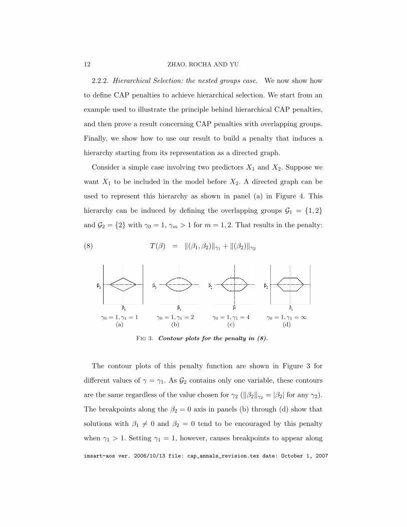
2.2.2. Hierarchical Selection: the nested groups case. We now show how

to define CAP penalties to achieve hierarchical selection. We start from an

example used to illustrate the principle behind hierarchical CAP penalties,

and then prove a result concerning CAP penalties with overlapping groups.

Finally, we show how to use our result to build a penalty that induces a

hierarchy starting from its representation as a directed graph.

Consider a simple case involving two predictors X1 and X2. Suppose we

want X1 to be included in the model before X2. A directed graph can be

used to represent this hierarchy as shown in panel (a) in Figure 4. This

hierarchy can be induced by defining the overlapping groups G1 = {1, 2}

and G2 = {2} with γ0 = 1, γm > 1 for m = 1, 2. That results in the penalty:

T (β) = ‖(β1, β2)‖γ1 + ‖(β2)‖γ2(8)

γ0 = 1, γ1 = 1 γ0 = 1, γ1 = 2 γ0 = 1, γ1 = 4 γ0 = 1, γ1 = ∞(a) (b) (c) (d)

Fig 3. Contour plots for the penalty in (8).

The contour plots of this penalty function are shown in Figure 3 for

different values of γ = γ1. As G2 contains only one variable, these contours

are the same regardless of the value chosen for γ2 (‖β2‖γ2 = |β2| for any γ2).

The breakpoints along the β2 = 0 axis in panels (b) through (d) show that

solutions with β1 6= 0 and β2 = 0 tend to be encouraged by this penalty

when γ1 > 1. Setting γ1 = 1, however, causes breakpoints to appear along



the β1 = 0 axis as shown in panel (a) hinting that γ1 > 1 is needed for the

hierarchical structure to be preserved.

In what refers to the definition of the groups, two things were important

for the hierarchy to arise from penalty (8): first, β2 was in every group β1

was; second, there was one group in which β2 was penalized without β1

being penalized. As we will see below, having β2 in every group where β1

is ensures that, once β2 deviates from zero, the infinitesimal penalty of β1

becomes zero. In addition, letting β2 be on a group of its own makes it

possible for β1 to deviate from zero, while β2 is kept at zero.

The general principle behind the example. The example above suggests

that, to construct more general hierarchies, the key is to set γ0 = 1, γk > 1

for all k. Given such a γ, a penalty can cause a set of indices I1 to be added

before the set I2, by defining groups G1 = I2 and G2 = I1 ∪ I2. Our next

result extends this simple case to more interesting hierarchical structures.

Theorem 1. Let I1, I2 ⊂ {1, . . . , p} be two subsets of indices. Suppose:

• γ0 = 1 and γk > 1,∀k = 1, . . . ,K

• I1 ⊂ Gk ⇒ I2 ⊂ Gk for all k and

• ∃k∗ such that I2 ⊂ Gk∗ and I1 6⊂ Gk∗

Then, ∂∂βI1

T (β) = 0 whenever βI2 6= 0 and βI1 = 0.

A proof is given in the Appendix. Assuming the set {Z ∈ Rn×(p+1) :

∂∂βI1

L(Z, β)∣∣∣βI2

=β̂I2,βI1

=0 = 0} to have zero probability, Theorem 1 states

that once the variables in I2 are added to the model, infinitesimal movements

of the coefficients of variables in I1 are not penalized and hence βI1 will

almost surely deviate from zero.



Defining groups for hierarchical selection. Using Theorem 1, a grouping for

a more complex hierarchical structure can be constructed from its represen-

tation as a directed graph. Let each node correspond to a group of variables

Gk and set its descendants to be the groups that should only be added to the

model after Gk. The graph representing the hierarchy in the simple case with

two predictors above is shown in the panel (a) of Figure 4. Based on this

representation and Theorem 1, CAP penalties enforcing the given hierarchy

can be obtained by setting:

T (β) =nodes∑m=1

αm ·∥∥∥(βGm , βall descendants of Gm

)∥∥∥γm

(9)

with αm > 0 for all m. The factor αm can be used to correct for the effect

of a coefficient being present in too many groups, a concern brought to our

attention by one of the referees. In this paper, we keep αm = 1 for all m

throughout. We return to this issue in our experimental section below.

For a more concrete example, consider a regression model involving d

predictors x1, . . . , xd and all its second order interactions. Suppose that an

interaction term xixj is to be added only after the corresponding main effects

xi and xj . The hierarchy graph is formed by adding an arrow from each main

effect to each of its interaction terms. Figure 4 shows the hierarchy graph

for d = 4. Figure 5 shows sample paths for d = 4 with penalties based on (9)

and using this hierarchy graph and having different settings for γk. These

sample paths were obtained by setting β1 = 20, β2 = 10, β3 = 5, β1,2 = 15

and β2,3 = 7. All remaining coefficients in the model are set to zero. Each

predictor has standard normal distribution and the signal to noise ratio is

set to 2. Because of the large effect of some interaction terms they are added

to the model before their respective main effects when the LASSO is used.



However, setting γk to be slightly larger than one is already enough to cause

the hierarchical structure to be satisfied. We develop this example further

in one of the simulation studies in Section 4.

(a) (b)

Fig 4. Directed graphs representing hierarchies: (a) The hierarchy of the simpleexample: X1 must precede X2; (b) Hierarchy for a main and interaction effects model withfour variables. The “root nodes” correspond to the main effects and must be added to themodel before its children. Each main effect has all the interactions in which it takes partas its children. Each second order interaction effect has two parents.

3. Computing CAP Estimates. The proper value of the regulariza-

tion parameter λ to use with CAP penalties is rarely known in advance. Two

ingredients are then needed to implement CAP in practice: efficient ways of

computing estimates for different values of λ and a criterion for choosing an

appropriate λ. This section proposes methods for completing these tasks.

3.1. Tracing the CAP regularization path. Convexity is a key property

for solving optimization problems such as the one defining CAP estimates

(7). When the objective function is convex, a point satisfying the Karush-

Kuhn-Tucker (KKT) conditions is necessarily a global minimum (see for

instance [2]). As the algorithms we present below rely on tracing solutions

to the KKT conditions for different values of λ, we now present sufficient

conditions for convexity of the CAP program (7). A proof is given in Ap-

pendix A.



γk ≡ 1 γk ≡ 1.1 γk ≡ 2 γk ≡ 4 γk ≡ ∞

(a) (b) (c) (d)

Fig 5. A sample regularization path for the simple ANOVA example with fourvariables In the LASSO path, an interaction (dotted lines) is allowed to enter the modelwhen its corresponding main effect (solid lines) is not in the model. When the group normγk is greater than one, the hiearchy is respected. From left to right: (a) Lasso (γ0 =1, γk ≡ 1); (b) CAP(1.1), (γ0 = 1, γk ≡ 4), (c) GLasso (γ0 = 1, γk ≡ 2), (d) CAP(4),(γ0 = 1, γk ≡ 4), (e) iCAP, (γ0 = 1, γk ≡ ∞).

Theorem 2. If γi ≥ 1,∀i = 0, ...,K, then T (β) in (6) is convex. If,

in addition, the loss function L is convex in β the objective function of the

CAP optimization problem in (7) is convex.

We now detail algorithms for computing the CAP regularization path.

The BLasso algorithm is used to deal with general convex loss functions and

CAP penalties. Under the L2-loss with γ0 = 1 and γk ≡ ∞, we introduce the

iCAP (∞-CAP) and the hiCAP (hierarchical-∞-CAP) algorithms to trace

the path for group and tree-structured hierarchical selection respectively.

3.1.1. The BLasso algorithm. The BLasso algorithm [24] can be used

to approximate the regularization path for general convex loss and penalty

functions. We use the BLasso algorithm in our experimental section due

to its ease of implementation and flexibility: the same code was used for

different settings of the CAP penalty.

Similarly to boosting [10] and the Forward Stagewise Fitting algorithm

[8], the BLasso algorithm works by taking forward steps of fixed size in the

direction of steepest descent of the loss function. However, BLasso also allows



for backward steps that take the penalty into account. With the addition

of these backward steps, the BLasso is proven to approximate the Lasso

path arbitrarily close, provided that the step size can get small. An added

advantage of the algorithm is its ability to trade off between precision and

computational expense by adjusting the step size. For a detailed description

of the algorithm, we refer the reader to Zhao and Yu [24].

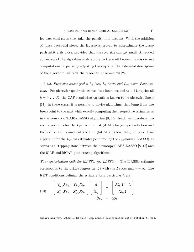
3.1.2. Piecewise linear paths: L2-loss, L1-norm and L∞-norm Penaliza-

tion. For piecewise quadratic, convex loss functions and γk ∈ {1,∞} for all

k = 0, . . . ,K, the CAP regularization path is known to be piecewise linear

[17]. In these cases, it is possible to devise algorithms that jump from one

breakpoint to the next while exactly computing their respective estimates as

in the homotopy/LARS-LASSO algorithm [8, 16]. Next, we introduce two

such algorithms for the L2-loss: the first (iCAP) for grouped selection and

the second for hierarchical selection (hiCAP). Before that, we present an

algorithm for the L2-loss estimates penalized by the L∞-norm (iLASSO). It

serves as a stepping stone between the homotopy/LARS-LASSO [8, 16] and

the iCAP and hiCAP path tracing algorithms.

The regularization path for iLASSO (∞-LASSO). The iLASSO estimate

corresponds to the bridge regression (2) with the L2-loss and γ = ∞. The

KKT conditions defining the estimate for a particular λ are: X ′RλXRλ

XRλXUλ

X ′UλXRλ

X ′Uλ

XUλ

α̂

β̂Uλ

=

X ′Rλ

Y − λ

XUλY

β̂Rλ

= α̂Sλ

(10)



whereRλ = {j : |β̂j | = ‖β̂‖∞}, Uλ = {j : |β̂j | < ‖β̂‖∞}, S(λ) = signs[X ′(Y−

Xβ̂(λ))], and XRλ=∑

j∈RλSj(λ)Xj . From these conditions, it follows that

|β̂j(λ)| = α̂, for all j ∈ Rλ and X ′j(Y −Xβ̂(λ)) = 0, for all j ∈ Uλ. Starting

from a breakpoint λ0 and its respective estimate β̂(λ0), the path moves in

a direction ∆β̂ that preserves the KKT conditions. The next breakpoint is

then determined by β̂λ1 = β̂λ0 + δ · ∆β̂ where δ > 0 is the least value to

cause an index to move between the Rλ and Uλ sets. The pseudo-code for

the iLASSO algorithm is presented in the technical report version of this

paper [23]. We now extend this algorithm to handle the grouped case.

The iCAP algorithm (∞-CAP). The iCAP algorithm is valid for the L2-

loss and non-overlapping groups with γ0 = 1 and γk ≡ ∞. This algorithm

operates on two levels: it behaves as the Lasso on the group level and as

the iLASSO within each group. To make this precise, first define the k-th

group correlation at λ to be ck(λ) = ‖X ′Gk

(Y − Xβ(λ))‖1 and the set of

active groups Aλ = {j ∈ {1, . . . ,K} : |cj(λ)| = maxk=1,...,K |ck(λ)|}. At

a given λ, the groups not in Aλ have all their coefficients set to zero and

β̂(λ) is such that all groups in Aλ have the same group correlation size. At

the within-group level, for β̂(λ) to be a solution, each index j ∈ Gk must

belong to either of two sets: Uλ,k = {j ∈ Gk : X ′j(Y − Xβ̂(λ)) = 0} and

Rλ,k = {j ∈ Gk : β̂j(λ) = ‖β̂Gk(λ)‖∞}.

For λ0 = maxj∈∞,...,K ‖X ′Gj

Y ‖1, the solution is given by β̂(λ0) = 0. From

this point, a direction ∆β̂ can be found so that the conditions above are

satisfied by β̂(λ0) + δ∆β̂ for small enough δ > 0. To find the next break-

point, compute the least value of δ > 0 that causes one of the following

events: a group is added to or removed from Aλ; an index moves between



the sets Uλ,k and Rλ,k for some group k; or a sign change occurs in the

correlation between the residuals and a variable in an inactive group. If

no such δ > 0 exists, the algorithm moves towards an un-regularized so-

lution along the direction ∆β̂. The pseudo-code is given in Appendix B.

The Matlab code implementing this algorithm can be downloaded from


The hiCAP algorithm (hierarchical-∞-CAP). We now introduce an algo-

rithm for hierarchical selection. It is valid for the L2-loss when γ0 = 1,

γk ≡ ∞ and the graph representing the hierarchy is a tree. The KKT con-

ditions in this case are to an extent similar to those of the non-overlapping

groups case. The difference is that the groups now change dynamically along

the path. Specifics of the algorithm are lengthy to describe and do not pro-

vide much statistical insight. We give a high level description here and refer

readers interested in implementing the algorithm to the code available at


The algorithm starts by forming non-overlapping groups such that:

• Each non-overlapping group consists of a sub-tree.

• Viewing each of the subtrees formed as a supernode, the derived super-

tree formed by these supernodes must satisfy the condition that aver-

age correlation size (unsigned) between Y and X’s within the supern-

ode is higher than that of all its descendant supernodes.

Once these groups are formed, the algorithm starts by moving the coef-

ficients in the root group as in the non-overlapping iCAP algorithm. The

optimality conditions are met because the root group has the highest average

correlation. Then, the algorithm proceeds observing two constraints:



1. Average unsigned correlation between Y −Xβ̂(λ) and X’s within each

supernode is at least as high than that of all its descendant supernodes;

2. Maximum unsigned coefficient of each supernode is larger than or equal

to that of any of its descendants;

Between breakpoints, the path is found by determining a direction such

that these conditions are met. Breakpoints are found by noticing they are

characterized by:

• If the average correlation between Y − Xβ̂(λ) and a subtree Ga con-

tained by a supernode equals that of a supernode, then Ga splits into

a new supernode.

• If a supernode a’s maximum coefficient size equals that of a descendant

supernode b, then they are combined into a new supernode. These

would also guarantee that a super node with all zero coefficients should

have descendants with all zero coefficients.

• If a supernode with all zero coefficients and a descendant reached equal

average correlation size (unsigned), they are merged.

3.2. Choosing the regularization parameter λ. For the selection of the

regularization parameter λ under general CAP penalties, we propose the

use of cross-validation. We refer the reader to Stone [19] and Efron [6] for

details on cross-validation. For the particular case of the iCAP having non-

overlapping groups and under the L2-loss, we extend Zou et al. [26]’s un-

biased estimate of the degrees of freedom for the LASSO. This estimate

can then be used in conjunction with an information criterion to pick an

appropriate level of regularization. We choose to use Sugiura’s AICC [20]



information criterion. Our preference for this criterion follows from its being

a correction of Akaike’s AIC [1] for small samples. Letting k denote the

dimensionality of a linear model, the AICC criterion for a linear model is:

AICC =n

2log

(n∑

i=1

(Yi −Xiβ̂(λ)

)2)

+n

2

(1 + k

n

1− k+2n

),(11)

where n corresponds to the sample size. A model is selected by minimizing

the expression in (11). To apply this criterion to iCAP, we substitute k by

estimates of the effective number of parameters (degrees of freedom). As we

will see in our experimental section, the AICC criterion resulted in good

predictive performance even in the “small-n,large-p” setting.

The extension of Zou et al. [26] unbiased estimates of the degrees of free-

dom to iCAP follows from noticing that, between breakpoints, the LASSO,

iLASSO and iCAP estimates mimic the behavior of projections on linear

subspaces spanned by subsets of the predictor variables. It follows that stan-

dard results for linear estimates establish the dimension of the projecting

subspace as an unbiased estimate of the degrees of freedom of penalized

estimates in a broader set of penalties. Therefore, to compute unbiased es-

timates of degrees of freedom for the iLASSO or iCAP regressions above,

it is enough to count of the number of free parameters at a point on the

path. Letting Aλ and Uk,λ be as defined in Section 3.1 above, the resulting

estimates of the degrees of freedom are d̂f(λ) = |Uλ|+1 for the iLASSO and

d̂f(λ) = |Aλ|+∑

k∈Aλ|Uk,λ| for the iCAP. A complete proof for the iLASSO

case and a sketch of the proof for the iCAP case are given in Appendix A.1.

Based on the above reasoning, we believe similar results should hold under

the L2-loss for any CAP penalties built exclusively from the L1-norm and

the L∞-norm. The missing ingredient is a way of determining the dimension



of a projecting subspace along the path in broader settings. Future research

will be devoted to that.

4. Experimental results. We now illustrate and evaluate the use of

CAP in a series of simulated examples. The CAP framework needs the input

of a grouping or hierarchical structure. For the grouping simulations, we

explore the possibility of having a data driven group structure choice and

show that CAP enjoys a certain degree of robustness to misspecified groups.

We leave a completely data driven group structure choice as a topic of future

research. For the hierarchical selection two examples illustrate the use of the

framework presented in Section 2.2.2 and the penalty in (9) to induce a pre-

determined hierarchy. We defer the study of data defined hierarchies for

future work.

We will be comparing the predictive performance, sparsity and parsimony

of different CAP estimates and that of the LASSO. As a measure of predic-

tion performance we use the model error ME(β̂) = (β̂ − β)E(X ′X)(β̂ − β).

In what concerns sparsity, we look not only at the number of variables se-

lected by CAP and LASSO, but also at measures of sparsity that take the

added structure into account: the number of selected groups for group se-

lection and a properly defined measure for hierarchical selection (see 4.2).

Whenever possible, we also compare the parsimony of the selected mod-

els as measured by the effective degrees of freedom and compare the cross

validation and AICC based selections for the tuning parameter λ.

In all experiments below, the data is simulated from:

Y = Xβ + σε,(12)



with ε ∼ N (0, I). The parameters β, σ as well as the covariance structure of

X are set specifically for each experiment.

4.1. Grouped selection results. In our grouping experiments, the group

structure among the p predictors in X is due to their relationship to a set

of K zero-mean Gaussian hidden factors Z ∈ RK :

cov(Zk, Zk′) =

2.0, if |k − k′| = 0,

1.0, if |k − k′| = 1,

0.0, if |k − k′| > 1,

for k, k′ ∈ {1, . . . ,K}.

A predictor Xj in group Gk is the sum of the Zk factor and a noise term:

Xj = Zk + ηj , if j ∈ Gk,

with the Gaussian ηj noise term having zero mean and:

cov(ηj , ηj′) = (4.0) · 0.95|j−j′|

The correlation between the factors Z is meant to make group selection

slightly more challenging. Also, we chose the covariance structure of the dis-

turbance terms η to avoid an overly easy case for the empirical determination

of the groups described below.

Clustering for forming groups. In applications, the grouping structure must

often be estimated from data. In our grouping experiments, we estimate the

true group structure G by clustering the predictors in X using the Partition-

ing Around Medoids (PAM) algorithm [see 13]. The PAM algorithm needs

the number of groups as an input. Instead of trying to fine tune the selection

of the number of groups, we fix the number of groups K̃ in the estimated

clustering above, below and at the correct value K. Specifically, we set:



• K̃ = K: proper estimation of the number of groups;

• K̃ = 0.5 ·K: severe underestimation of the number of groups;

• K̃ = 1.5 ·K: severe overestimation of the number of groups;

Implicitly, we are assuming that a tuning method that can set the number

of estimated groups K̃ in PAM to be between 0.5K (alt. below 1.5K) and

the true number of groups K has results that are no worse than the ones

observed in our underestimated (alt. overestimated) scenarios.

4.1.1. Effect of group norms and λ selection methods. In this first ex-

periment, we want to compare the difference amongst CAP estimates using

alternative settings for the within group norm and the LASSO. We keep the

dimensionality of the problem low and emulate a high-dimensional setting

(n < p) by setting

n = 80, p = 100, and K = 10.

The coefficients β are made dissimilar (see Figure 6) within a group to

avoid undue advantage to iCAP:

βj =

0.10(1 + 0.9j−1), for j = 1, . . . , 10;

0.04(1 + 0.9j−11), for j = 11, . . . , 20;

0.01(1 + 0.9j−21), for j = 21, . . . , 30;

0, otherwise.

The noise level is set to σ = 3 and results are based on 50 replications.

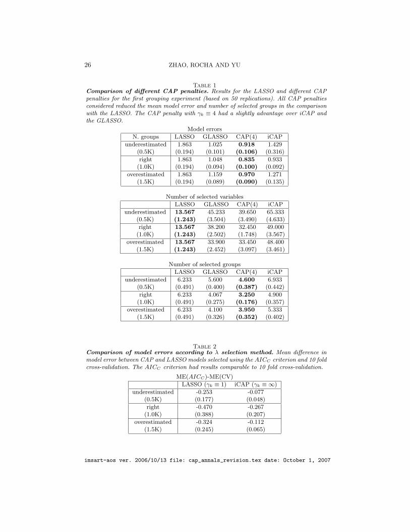
The results reported in Table 1 show that all the different CAP penalties

considered significantly reduced the model error in the comparison with the

LASSO. The reduction in model error was also observed to be robust to mis-

specifications of the group structure (the cases K̃ = 0.5 ·K and K̃ = 1.5 ·K).



Table 2 shows that our estimate for the degrees of freedom used in con-

junction with the AICC criterion was able to select predictive models as good

as 10-fold cross-validation at a lower computational expense. The compari-

son of the results across the number of clusters used to group the predictors

show that the improvement in prediction was robust to misspecifications in

the number of groups used to cluster the predictors. iCAP’s performance was

the most sensitive to this type of misspecification as the L∞-norm makes a

heavier use of the prespecified grouping information.

In terms of sparsity, the CAP estimates include a larger number of vari-

ables than the LASSO due to its block-inclusion nature. If we look at how

many of the true groups are selected instead, we see that the CAP estimates

made use of a lesser number of groups that the LASSO: an advantage if

group selection is the goal. The low ratio between the average number of

variables and the average number of groups selected by the LASSO provide

evidence that the LASSO estimates did not preserve the group structure

selecting only a few variables from each group.

Fig 6. Profile of coefficients for grouping experiment In the first grouping experi-ment, only the first three groups have non-zero coefficients. Within each group, the coeffi-cients have an exponential decay.



Table 1Comparison of different CAP penalties. Results for the LASSO and different CAPpenalties for the first grouping experiment (based on 50 replications). All CAP penaltiesconsidered reduced the mean model error and number of selected groups in the comparisonwith the LASSO. The CAP penalty with γk ≡ 4 had a slightly advantage over iCAP andthe GLASSO.

Model errors

N. groups LASSO GLASSO CAP(4) iCAP

underestimated 1.863 1.025 0.918 1.429(0.5K) (0.194) (0.101) (0.106) (0.316)

right 1.863 1.048 0.835 0.933(1.0K) (0.194) (0.094) (0.100) (0.092)

overestimated 1.863 1.159 0.970 1.271(1.5K) (0.194) (0.089) (0.090) (0.135)

Number of selected variables

LASSO GLASSO CAP(4) iCAP


right 13.567 38.200 32.450 49.000(1.0K) (1.243) (2.502) (1.748) (3.567)

overestimated 13.567 33.900 33.450 48.400(1.5K) (1.243) (2.452) (3.097) (3.461)

Number of selected groups

LASSO GLASSO CAP(4) iCAP


right 6.233 4.067 3.250 4.900(1.0K) (0.491) (0.275) (0.176) (0.357)

overestimated 6.233 4.100 3.950 5.333(1.5K) (0.491) (0.326) (0.352) (0.402)

Table 2Comparison of model errors according to λ selection method. Mean difference inmodel error between CAP and LASSO models selected using the AICC criterion and 10 foldcross-validation. The AICC criterion had results comparable to 10 fold cross-validation.

ME(AICC)-ME(CV)

LASSO (γk ≡ 1) iCAP (γk ≡ ∞)

underestimated -0.253 -0.077(0.5K) (0.177) (0.048)

right -0.470 -0.267(1.0K) (0.388) (0.207)

overestimated -0.324 -0.112(1.5K) (0.245) (0.065)



4.1.2. Grouping with small-n-large-p. We now compare iCAP and the

LASSO when the number of predictors p = Kq grows due to an increase

in either the number of groups K or in the group size q. The sample size

is fixed at n = 80. The coefficients are randomly selected for each replica-

tion according to two different schemes: in the Grouped Laplacian scheme

the coefficients are constant within each group and equal to K independent

samples from a Laplacian distribution with parameter αG; in the Individ-

ual Laplacian scheme the p coefficients are independently sampled from a

Laplacian distribution with parameter αI . The Grouped Laplacian scheme

favors iCAP due to the grouped structure of the coefficients whereas the

Individual Laplacian scheme favors the LASSO. The parameters αG and αI

were adjusted so the signal power E(β′X ′Xβ) is roughly constant across

experiments. The complete set of parameters used is shown in Table 3.

We only report the results obtained from using the AICC criterion was

used to select λ. The results for 10-fold cross-validation were similar. Tables

4 and 5 show the results based on 100 replications.

The iCAP estimates had predictive performance better than or compa-

rable to LASSO estimates. For the Grouped Laplacian case, the reduction

in model error was very pronounced for all settings considered. In the Indi-

vidual Laplacian case, iCAP and LASSO had comparable model errors for

Table 3Parameters for the simulation of the small-n-large-p case.

Grouped Laplacian Individual Laplacianp q K αG E(β′X ′Xβ) SNR αI E(β′X ′Xβ) SNR σ

100 10 10 1.00 · 10−1 54.02 3.95 3.00 · 10−1 54.00 3.95 3.7250 10 25 0.63 · 10−1 53.60 3.92 1.90 · 10−1 54.15 3.96 3.7250 25 10 0.43 · 10−1 54.61 3.99 1.90 · 10−1 54.15 3.96 3.7



Table 4Results for small-n-large-p experiment under Grouped Laplacian sampling. Re-sults based on 100 replications and AICC selected λ. The true model has its parameterssampled according to the Grouped Laplacian scheme (see Section 4.1.2). The inclusion ofgrouping structure improves the predictive performance of the models whether the predic-tors are clustered in the correct number of groups (1.0K) or not (0.5K and 1.5K). LASSOselects a smaller number of variables and is slightly sparser in terms of number of groups.iCAP estimates are more parsimonious in terms of degrees of freedom.

Model errors

LASSO 0.5K 1.0 K 1.5K

p=100, q=10 5.028 3.783 2.839 3.481(0.208) (0.172) (0.119) (0.132)

p=250, q=10 13.061 11.135 6.660 8.128(0.506) (0.834) (0.227) (0.271)

p=250, q=25 8.356 5.113 3.479 4.457(0.379) (0.228) (0.149) (0.202)


LASSO 0.5K 1.0 K 1.5K

p=100, q=10 19.590 93.940 82.200 73.720(0.546) (1.108) (1.508) (1.438)

p=250, q=10 26.070 211.090 169.700 144.740(0.668) (3.335) (2.866) (2.781)

p=250, q=25 25.450 236.300 218.500 192.730(0.664) (2.979) (3.049) (3.667)

Number of true groups selected

LASSO 0.5K 1.0 K 1.5K

p=100, q=10 8.140 9.520 8.220 8.240(0.163) (0.090) (0.151) (0.148)

p=250, q=10 14.550 21.780 16.970 16.720(0.336) (0.290) (0.287) (0.317)

p=250, q=25 7.980 9.560 8.740 8.530(0.160) (0.102) (0.122) (0.149)

Degrees of freedom

LASSO 0.5K 1.0 K 1.5K

p=100, q=10 19.590 13.600 10.460 12.060(0.546) (0.459) (0.365) (0.404)

p=250, q=10 26.070 19.710 18.490 20.190(0.668) (0.646) (0.431) (0.501)

p=250, q=25 25.450 18.010 13.590 14.920(0.664) (0.604) (0.481) (0.491)



Table 5Results for small-n-large-p experiment under Individual Laplacian sampling. Re-sults based on 100 replications and AICC selected λ. The true model has its parameterssampled according to the Independent Laplacian scheme (see Section 4.1.2). For a lowerdimensional model (p = 100, q = 10), the predictive performance of iCAP is comparableto the LASSO. For higher-dimensions (p = 250, q = 10 and q = 25), iCAP has betterpredictive performance. LASSO selects a smaller number of variables than iCAP and acomparable number of groups in all cases. iCAP estimates are still more parsimonious interms of degrees of freedom.

Model errors

LASSO 0.5K 1.0 K 1.5K

p=100, q=10 10.310 10.885 10.153 11.056(0.309) (0.388) (0.300) (0.348)

p=250, q=10 22.560 18.790 18.194 18.990(0.701) (0.446) (0.463) (0.422)

p=250, q=25 19.891 17.483 16.544 18.301(0.614) (0.424) (0.387) (0.493)


LASSO 0.5K 1.0 K 1.5K

p=100, q=10 20.200 96.460 90.700 73.530(0.620) (0.869) (1.249) (1.459)

p=250, q=10 25.540 228.070 180.700 150.000(0.620) (2.246) (3.003) (2.508)

p=250, q=25 24.440 243.490 234.250 198.040(0.589) (1.530) (1.935) (2.638)

Number of true groups selected

LASSO 0.5K 1.0 K 1.5K

p=100, q=10 9.580 9.760 9.480 9.320(0.106) (0.092) (0.098) (0.119)

p=250, q=10 21.210 24.110 21.580 20.720(0.309) (0.115) (0.266) (0.290)

p=250, q=25 9.720 9.870 9.730 9.650(0.057) (0.049) (0.066) (0.069)

Degrees of freedom

LASSO 0.5K 1.0 K 1.5K

p=100, q=10 20.200 16.320 16.140 14.650(0.620) (0.684) (0.635) (0.614)

p=250, q=10 25.540 22.230 20.290 21.210(0.620) (0.630) (0.486) (0.536)

p=250, q=25 24.440 20.360 20.060 18.670(0.589) (0.610) (0.635) (0.637)



p = 100. As the number of predictors increased, however, iCAP resulted

in lower model errors than the LASSO even under the Individual Lapla-

cian regime. This result provides evidence that collecting highly-correlated

predictors into groups is benefitial in terms of predicting performance espe-

cially as the ratio p/n increases. The predictive gains from using CAP were

also preserved under mis-specified groupings. iCAP estimates had smaller

or comparable model errors than the LASSO when the predictors were clus-

tered into a number of groups that was 50% smaller or larger than the actual

number of predictor clusters.

Contrary to what was expected, the iCAP estimates involved a number

of groups comparable to the LASSO in all simulated scenarios. We believe

this is due to a more parsimonious use of degrees of freedom by iCAP esti-

mates. As more groups are added to the model, the within-group restrictions

imposed by the L∞-norm prevent a rapid increase in the use of degrees of

freedom. As a result, iCAP estimates can afford to include groups in the

model more agressively in an attempt to reduce the L2-loss. This reasoning

is supported by the lesser degrees of freedom used by iCAP selected models

in the comparison to the LASSO.

4.2. Hierarchical selection results. Now, we provide examples where the

hierarchical structure of the predictors is exploited to enhance the predictive

performance of models. We define hierarchical gap as a measure of compli-

ance to the given hierarchical structure: it is minimal number of additional

variables that should be added to the model so the hierarchy is satisfied. If

a model satisfies a given hierarchy, no additional variables must be added

and this measure equals zero.



4.2.1. Hierarchical selection for ANOVA model with interaction terms.

We now further develop the regression model with interaction terms intro-

duced in Section 2 (cf. Figure 4).

The data is generated according to (12) and set the number of variables to

d = 10 resulting in a regression involving 10 main effects and 45 interactions:

X = [Z1, . . . , Z10, Z1Z2, . . . , Z1Z10, . . . , Z9Z10]

Zji.i.d.∼ N (0, 1)

We assume the hierarchical structure is given that the second order terms

are to be added to the model only after their corresponding main effects.

This is an extension of the hierarchical structure in Figure 4 from d = 4 to

d = 10. Applying (9) to this graph with uniform αm weights gives:

T (β) =10∑

j=1

j−1∑i=1

[|βi,j |+ ‖(βi, βj , βi,j)‖γi,j

]In this case, each interaction term is penalized in three factors of the sum-

mation which agrees to the number of variables that are added to the model

(Zij , Zi and Zj).

We set the first four the main effect coefficients to be β1 = 7, β2 = 2, β3 =

1 and β4 = 1 with all remaining main effects set to zero. The main effects

are kept fixed throughout and five different levels of interaction strengths

are considered as shown in Table 6. The variance of the noise term was kept

constant across the experiments. The number of observations n was set to

121. The results reported in Table 7 were obtained from 100 replications.

For low and moderate interactions, the introduction of hierarchical struc-

ture reduced the model error from the LASSO. For strong interactions, the

CAP and LASSO results were comparable. For very strong interactions, the



Table 6Simulation setup for the ANOVA experiment.

CoefficientsDescription Z1Z2 Z1Z3 Z1Z4 Z2Z3 Z2Z4 Z3Z4 σ SNR

No interactions 0 0 0 0 0 0 3.7 4.02Weak interactions 0.5 0 0 0.1 0.1 0 3.7 4.08Moderate interactions 1.0 0 0 0.5 0.4 0.1 3.7 4.33Strong interactions 5 0 0 4 2 0 3.7 13.88Very Strong interactions 7 7 7 2 2 1 3.7 38.20

implicit assumption of smaller second order effects embedded in the hierar-

chical selection is no longer suitable causing the LASSO to reach a better

predictive performance.

In addition, CAP selected models involving on average a slightly lesser

or equal number of variables to the LASSO in all simulated cases. The

hierarchical gap (see definition in 4.2) for the LASSO shows that it did

not comply with the hierarchy of the problem. According to the theory

developed in Section 2, for CAP estimates this difference should be exactly

zero. The small deviations from zero observed in our experiments are due

to the approximate nature of the BLasso algorithm.

4.2.2. Multiresolution model. In this experiment, the true signal is given

by a linear combination of Haar wavelets at different resolution levels. Let-

ting Zij denote the Haar wavelet at the j-th position of level i, we have:

Zij(t) =

−1, if t ∈ ( j

2i+1 , j+12i+1 )

1, if t ∈ ( j+12i+1 , j+2

2i+1 )

0, otherwise

, for i ∈ N, j = 0, 1, 2, . . . , 2i−1

In what follows, we let a vector Z̃ij be formed by computing Zij(t) at 16

equally spaced “time points” over [0, 1]. The design matrix X is then given



Table 7Simulation results for the hierarchical ANOVA example. Results based on 50 repli-cations, 121 observations and 10 fold CV. Hierarchical structure lead to reduced modelerror and sparser models. The hierarchy gap is the number of variables that must be addedto the model so the hierarchy is satisfied. The LASSO does not respect the model hierarchy.The small deviations from zero for CAP estimates are due to BLASSO approximation.

Model errors

LASSO “GLASSO” CAP(4) iCAP

No Interactions 3.367 1.481 1.478 1.466(0.288) (0.133) (0.134) (0.124)

Weak Interactions 4.032 2.190 2.296 2.117(0.303) (0.147) (0.161) (0.117)

Moderate Interactions 5.905 4.260 4.090 4.085(0.307) (0.205) (0.207) (0.196)

Strong Interactions 8.912 8.901 7.793 8.388(0.695) (0.621) (0.568) (0.626)

Very Strong Int. 11.474 11.998 14.538 26.072(0.758) (0.800) (0.915) (1.351)



No Interactions 13.440 12.720 11.440 9.280(0.897) (0.935) (0.725) (0.431)

Weak Interactions 13.960 13.780 12.720 9.920(0.936) (1.041) (0.806) (0.442)



Very Strong Int. 26.400 28.020 20.520 14.560(0.670) (0.577) (0.448) (0.289)

Hierarchy gap


No Interactions 3.560 0.220 0.420 0.800(0.192) (0.066) (0.107) (0.128)

Weak interactionsI 3.560 0.160 0.340 0.840(0.169) (0.052) (0.079) (0.112)



Very Strong Int. 3.780 1.080 1.580 0.920(0.155) (0.140) (0.143) (0.137)



by:[

Z̃00 , Z̃10 Z̃11 , Z̃20 · · · Z̃23 , Z̃30 · · · Z̃37

].

We consider five different settings for the value of β with various sparsity

levels and tree depths. The parameter σ is adjusted to keep the signal to

noise ratio is at 0.4 in all cases. The true model parameters are shown within

the tree hierarchy in Figure 7.

The simulated data corresponds to 5 sets of observations of the 16 “time

points”. Five fold cross validation was used for selecting the regularization

level. At each cross-validation round, the 16 points kept out of the sample

correspond to each of the “time positions” (“balanced cross-validation”).

In its upper left panel, Figure 7 shows the directed graph representing the

tree hierarchy used to form the CAP penalty using the recipe laid out by

(9) in section 2 with αm = 1 for all m. Our option for setting all weights to

one in this case is similar to the one presented in the ANOVA experiment

above: the number of variables added to the model when a variable is added

matches the number of times its coefficient appears on the penalty.

The results for the hierarchical selection are shown in Table 8. The use

of the hierarchical information greatly reduced the model error as well as

the number of selected variables. As in the ANOVA cases, the hierarchical

gap shows that the LASSO models do not satisfy the tree hierarchy. The

approximate nature of the BLASSO algorithm again causes the hierarchi-

cal gap of GLASSO and CAP(4) to deviate slightly from zero. For hiCAP

estimates, perfect agreement with the hierarchy is observed as the hiCAP

algorithm (see Section 3) is exact.



Table 8Simulation results for the hierarchical wavelet tree example. Results based on 200replications, 5 × 16 observations and 5 fold “balanced” CV. Hierarchical structure leadto reduced model error and sparser models. The hierarchy gap is the number of variablesthat must be added to the model so the hierarchy is satisfied. The LASSO does not respectthe tree hiearchy. Small discrepancies in GLASSO and CAP(4) due to approximation inBLASSO.

Model errorsLASSO GLASSO CAP(4) iCAP

root-only tree 40.508 26.994 28.498 28.909(2.039) (1.635) (1.650) (1.820)

one-sided 80.197 57.100 58.228 57.195(2.954) (2.519) (2.465) (2.532)

complete tree 112.578 76.911 79.498 78.117(3.407) (2.661) (2.736) (2.733)

regular tree 82.979 58.020 60.037 60.259(2.738) (2.237) (2.252) (2.379)

heavy-leaved tree 454.607 388.262 385.770 359.154(11.950) (10.015) (9.884) (10.565)

Number of selected variablesLASSO GLASSO CAP(4) iCAP

root-only tree 4.070 4.495 4.405 3.185(0.209) (0.265) (0.241) (0.244)

one-sided 6.080 6.770 6.235 5.415(0.211) (0.247) (0.218) (0.245)

complete tree 7.010 7.605 6.995 6.720(0.226) (0.227) (0.213) (0.248)

regular tree 6.140 6.690 6.255 5.490(0.230) (0.243) (0.218) (0.250)


Hierarchy gapLASSO GLASSO CAP(4) iCAP

root-only tree 1.765 0.235 0.360 0.000(0.096) (0.038) (0.049) (0.000)

one-sided 0.710 0.180 0.300 0.000(0.064) (0.031) (0.038) (0.000)

complete tree 1.640 0.310 0.505 0.000(0.091) (0.042) (0.057) (0.000)

regular tree 1.210 0.225 0.335 0.000(0.069) (0.030) (0.039) (0.000)




case 1 (σ = 23.72, SNR= 0.4) case 2 (σ = 26.86, SNR= 0.4)root-only tree one-sided tree

case 3 (σ = 28.52, SNR= 0.4) case 4 (σ = 27.08, SNR= 0.4)almost-complete tree regular tree

case 5 (σ = 47.43, SNR= 0.4)deep tree

Fig 7. Coefficients and hierarchies used in the wavelet tree example.

4.3. Additional experiments. In addition to the experiments presented

above, we have also run CAP under examples taken from Yuan and Lin

[22] and Zou and Hastie [25]. The results are similar to the ones obtained

above: CAP results in improved prediction performance over the LASSO

with models involving a larger number of variables, a similar or smaller

number of groups and making use of less degrees of freedom. We invite the

reader to check the details in the technical report version of this paper [23].



5. Discussion and Concluding Remarks. In this paper, we have

introduced the Composite Absolute Penalty (CAP) family. It provides a

regularization framework for incorporating pre-determined grouping and hi-

erarchical structures among the predictors by combining Lγ-norm penalties

and applying them to properly defined groups of coefficients.

The definition of the groups to which norms are applied is instrumental

in determining the properties of CAP estimates. Non-overlapping groups

give rise to group selection as done previously by Yuan and Lin [22] and

Kim et al. [14] where L1 and L2 norms are combined. CAP penalties extend

these works by letting norms other than the L2-norm to be applied to the

groups of variables. Combinations of the L1 and L∞ are convenient from

a computational standpoint as illustrated by the iCAP (non-overlapping

groups) with fast homotopy/LARS-type algorithms. Its Matlab code can be

downloaded from our research group website:


The definition of CAP penalties also generalizes previous work by allowing

the groups to overlap. Here, we have shown how to construct overlapping

groups leading to hierarchical selection. Combinations of the L1 and L∞ are

also computationally convenient to hierarchical selection as illustrated by

the hiCAP algorithm for tree hierarchical selection (also available from our

research group website).

In a set of simulated examples, we have shown that CAP estimates us-

ing a given grouping or hierarchical structure can reduce the model error

when compared to LASSO estimates. In the grouped selection case, we show

such reduction has taken place in the “small-n-large-p” setting and was ob-



served even when the groups were data-determined (noisy) and the resulting

number of groups was within a large margin of the actual number of groups

among the predictors (between 50% and 150% of the true number of groups).

In addition, iCAP predictions are more parsimonious in terms of use of

degrees of freedom being less sensitive to disturbances in the observed data

[7]. Finally, CAP’s ability to select models respecting the group and hier-

archical structure of the problems makes its estimates more interpretable.

It is a topic of our future research to explore ways to estimate group and

hierarchical structures completely based on data.

A. Appendix: Proofs.

Proof. of Theorem 1. Algebraically, we have for γ > 1:

∂

∂β1T (β) =

∂

∂β1‖β‖γ = sign (β1)

(|β1|‖β‖γ

)(γ−1)

As a result, if β2 > 0, β1 is locally not penalized at 0 and it will only stay

at this point if the gradient of the loss function L is exactly zero for β1 = 0.

Unless the distribution of the gradient of the loss function has an atom at

zero for β1, β1 6= 0 with probability one.

Proof. of Theorem 2. It is enough to prove that T is convex:

1. T(α · β) = |α| ·T(β), for all α ∈ R: For each group k, Nk(αβ) =

αNk(β). Thus T (αβ) = ‖N(αβ)‖γ0 = |α|‖N(β)‖γ0 = |α|T (β);

2. T(β1 + β2) ≤ T(β1) + T(β2): Using the triangular inequality:

T (β1 + β2) =∑k

(Nk(β1 + β2))γ0 ≤

∑k

(Nk(β1) + Nk(β2))γ0

= ‖N(β1) + N(β2)‖γ0 ≤ ‖N(β1)‖γ0 + ‖N(β2)‖γ0

= T (β1) + T (β2)



Convexity follows by setting β1 = θβ3 and β2 = (1−θ)β4 with θ ∈ [0, 1].

A.1. DF Estimates for iLASSO and iCAP. We now derive an unbiased

estimate for the degrees of freedom of iLASSO fits along the regularization

path. The optimization problem defining the iLASSO estimate is dual to the

LASSO problem (see for instance [2]). Facts 1 through 3 below follow from

this duality and the results in Efron et al. [8] and Zou et al. [26]. In what

follows, we denote the iLASSO and iCAP fit by µ̂(λ, y) = Xβ̂(λ, y).

Fact 1. For each λ, there exists a set Kλ such that Kλ is a the union

of a finite collection of hyperplanes and for all Y ∈ Cλ = Rn −Kλ, λ is not

a breakpoint in the regularization path.

Fact 2. β̂(λ, y) is a continuous function of y for all λ.

Fact 3. If y ∈ Cλ, then the sets Rλ and Uλ are locally invariant.

From these three facts, we can prove:

Lemma 1. For a fixed λ ≥ 0 and Y ∈ Cλ , µ̂(λ, y) satisfies:

‖µ̂(λ, y + ∆y)− µ̂(λ, y)‖ ≤ ‖∆y‖, for sufficiently small ∆y and

∇ · µ̂(λ, y) = |Uλ|+ 1

Proof. Lemma 1 We first notice that, µ̂(λ, y) = Xβ̂(λ, Y ) =[XRλ

XUλ

]·[

α̂ β̂′Uλ

]′. From the optimality conditions for the L∞ penalty:

(X ′X

)α̂(λ, Y ) = X ′Y − λ · sign (Y −X α̂(λ, Y )) , and(

X ′X)α̂(λ, Y + ∆Y ) = X ′(Y + ∆Y )− λ · sign (Y + ∆Y −X α̂(λ, Y + ∆Y ))



For Y ∈ Cλ, there exists small ∆Y so the signs of the the correlation

between the residuals and each predictor are preserved. Subtracting the two

equations above: µ̂(λ, Y +∆Y )−µ̂(λ, Y ) = X (X ′X )−1X ′∆Y . Thus, µ̂(λ, Y )

behaves locally as a projection on a fixed subspace implied by Rλ and Uλ.

From standard projection matrix results: ‖Xβ̂(λ, y + ∆y) − Xβ̂(λ, y)‖ ≤

‖∆y‖, for small ∆y and ∇ · µ̂(λ, Y ) = tr(X (X ′X )−1X ′) = |Uλ|+ 1.

Lemma 1 implies that the fit µ̂(λ, y) is uniformly Lipschitz on Rn (it is

the closure of Cλ). Using Stein’s lemma and the divergent expression above:

Theorem 3. The L∞-penalized fit µ̂λ(y) is uniformly Lipschitz for all

λ. The degrees of freedom of µ̂λ(y) is given by df(λ) = E [|Uλ|] + 1.

The proof for the case of non-overlapping groups follows the same steps.

We only present a sketch of the proof as a detailed proof is not very insight-

ful. Fact 1 is proven by noticing that, for fixed λ, each of the conditions

defining breakpoints require Y to belong to a finite union of hyperplanes.

Fact 2 follows from the CAP objective function being convex and contin-

uous in both λ and Y . Fact 3 is established by noticing that the sets Aλ

and Rk,λ,∀k = 1, . . . ,K are invariant in between breakpoints. As before,

the CAP fit behaves (except for a shrinkage factor) as a projection onto a

subspace whose dimension is the number of “free” parameters at that point

of the path. The result follows from standard arguments for linear estimates.

B. Pseudo-code for the iCAP algorithm.

1. Set t = 0, λt = maxk ‖ck(0)‖, β̂(λt) = 0

2. Repeat until λt = 0:



(a) Set Aλt to contain all groups with ck = λt;

(b) For each group k, set :

Uλ,k = {j ∈ Gk : X ′j(Y −Xβ̂(λt)) = 0} and Rλ,k = Gk − Uk,λ;

(c) Determine a direction ∆β̂ such that:

i. if k 6∈ Aλ, then ∆β̂Gk= 0;

ii. for k ∈ Aλ, ∆β̂Rk,λ= αk · Sλ,k with αk chosen so:

ck(β̂(λ) + δ ·∆β̂) = ck∗(β̂(λ) + δ ·∆β̂) for all k, k∗ ∈ Aλ and ,

X ′Uk,λ

(Y −X(β̂(λ) + δ ·∆β̂)

)= 0 for small enough δ > 0;

(d) Compute the step sizes for which breakpoints occur:

δA = infδ>0

{ck∗(β̂λ + δ ·∆β̂) = ck(β̂λ + δ ·∆β̂) for some k∗ 6∈ Aλ and k ∈ Aλ

};

δI = infδ>0

{‖β̂Gk

(λ) + δ ·∆β̂‖∞ = 0 for some k ∈ Aλ

}δU = inf

δ>0

{X ′

m

(Y −X(β̂(λ) + δ ·∆β̂)

)= 0 for some m ∈ Gk with k ∈ Aλ

}δR = inf

δ>0

{|β̂m(λ) + δ ·∆β̂m| = ‖β̂Gk

(λ) + δ ·∆β̂‖∞ for some m ∈ Uk,λ with k ∈ Aλ

}δS = inf

δ>0

{X ′

m

(Y −X(β̂(λ) + δ ·∆β̂)

)= 0 for some m ∈ Gk with k 6∈ Aλ

}where we take the infimum over an empty set to be +∞.

(e) Set t = t+1, δ = min{δA, δI , δR, δU , δS , λt}, λt+1 = ‖ck

(β̂(λt) + δ ·∆β̂

)‖∞

and β̂(λt+1) = β̂(λt) + δ ·∆β̂

References.

[1] Akaike, H. 1973. Information theory and an extension of the maximum likelihood

principle. Proc. 2nd International Symposium on Information Theory , 267–281.

[2] Boyd, S. and Vandenberghe, L. 2004. Convex Optimization. Cambridge University

Press.



[3] Breiman, L. 1995. Better subset regression using the nonnegative garrote. Techno-

metrics 37, 4, 373–384.

[4] Chen, S. S., Donoho, D. L., and Saunders, M. A. 2001. Atomic decomposition

by basis pursuit. SIAM Review 43, 1, 129–159.

[5] Donoho, D. and Johnstone, I. 1994. Ideal spatial adaptation by wavelet shrinkage.

Biometrika 81, 3 (August), 425–455.

[6] Efron, B. 1982. The Jackknife, the Bootstrap and Other Resampling Plans. Society

for Applied and Industrial Math.

[7] Efron, B. 2004. The estimation of prediction error covariance penalties and cross-

validation. Journal of the American Statistical Association 99, 467, 619–632.

[8] Efron, B., Hastie, T., Johnstone, I., and Tibshirani, R. 2004. Least angle re-

gression. The Annals of Statistics 35, 407–499.

[9] Frank, I. E. and Friedman, J. 1993. A statistical view of some chemometrics

regression tools. Technometrics 35, 109–148.

[10] Freund, Y. and Schapire, R. E. 1997. A decision theoretic generalization of on-line

learning and an application to boosting. Journal Computer and System Sciences 55,

119–139.

[11] Golub, T. R., Slonim, D. K., Tamayo, P., Huard, C., Gaasenbeek, M.,

Mesirov, J. P., Coller, H., Loh, M. L., Downing, J. R., Caligiuri, M. A.,

Bloomfield, C. D., and Lander, E. S. 1999. Molecular classification of cancer: Class

discovery and class prediction by gene expression monitoring. Science 286, 531–537.

[12] Hoerl, A. E. and Kennard, R. W. 1970. Ridge regression: Biased estimation of

nonorthogonal problems. Technometrics 12, 1, 55–67.

[13] Kaufman, L. and Rousseeuw, P. J. 1990. Finding groups in data: an introduction

to cluster analysis. John Wiley & Sons.

[14] Kim, Y., Kim, J., and Kim, Y. 2006. Blockwise sparse regression. Statistica

Sinica 16, 2, 375–390.

[15] Mallows, C. L. 1973. Some comments on cp. Technometrics 15, 4, 661–675.

[16] Osborne, M., Presnell, B., and Turlach, B. 2000. A new approach to variable

selection in least square problems. IMA Journal of Numeric Analysis 20, 389–404.

[17] Rosset, S. and Zhu, J. 2004. Piecewise linear regularized solution paths. Tech.



rep., University of Michigan Department of Statistics.

[18] Schwartz, G. 1978. Estimating the dimension of a model. The Annals of Statistics 6,

461–464.

[19] Stone, M. 1974. Cross-validatory choice and assessment of statistical predictions.

Journal of the Royal Statistical Society. Series B (Methodological) 36, 2, 111–147.

[20] Sugiura, N. 1978. Further analysis of the data by akaike’s information criterion and

finite corrections. Communications in Statistics A7, 1, 13–26.

[21] Tibshirani, R. 1996. Regression shrinkage and selection via the lasso. Journal of

the Royal Statistical Society, Series B 58, 1, 267–288.

[22] Yuan, M. and Lin, Y. 2006. Model selection and estimation in regression with

grouped variables. Journal of the Royal Statistical Society, Series B 68, 1, 49–67.

[23] Zhao, P., Rocha, G., and Yu, B. 2006. Grouped and hierarchical model selec-

tion through composite absolute penalties. Tech. rep., Department of Statistics, UC

Berkeley.

[24] Zhao, P. and Yu, B. 2004. Boosted lasso. Tech. rep., Department of Statistics, UC

Berkeley.

[25] Zou, H. and Hastie, T. 2005. Regularization and variable selection via the elastic

net. Journal of the Royal Statistical Society, Series B 67, 2, 301–320.

[26] Zou, H., Hastie, T., and Tibshirani, R. 2004. On the “degrees of freedom” of the

lasso. Tech. rep., Stanford University Department of Statistics.

Department of Statistics

University of California, Berkeley

367 Evans Hall

Berkeley, CA 94720

USA

E-mail: [email protected]




the composite absolute penalties family for grouped …

Documents