the cosmological constant problem and many-body physics …
TRANSCRIPT
The Pennsylvania State University
The Graduate School
Eberly College of Science
THE COSMOLOGICAL CONSTANT PROBLEM
AND
MANY-BODY PHYSICS: AN INVESTIGATION
A Dissertation inPhysics
byDeepak Vaid
Submitted in Partial Fulfillmentof the Requirements
for the Degree of
Doctor of Philosophy
May 2012

The dissertation of Deepak Vaid was reviewed and approved* by the following:
Stephon AlexanderAssociate Professor of Physics, Haverford CollegeCo-Chair of CommitteeDissertation Adviser
Martin BojowaldAssociate Professor of PhysicsCo-Chair of Committee
Jainendra JainErwin W. Mueller Professor of Physics
Adrian OcneanuProfessor of Mathematics
Nitin SamarthProfessor of PhysicsGeorge A. and Margaret M. Downsbrough Department Head of Physics
*Signatures are on file in the Graduate School.

Abstract
A model for condensation of fermions in a flat Friedmann-Robertson-Walker (FRW) back-
ground is presented. It is shown that condensation can happen, via the BCS mechanism
due to a four-fermion interaction which appears naturally when fermions are included in
gravity. We argue that this process can form the basis for a non-perturbative resolution to
the cosmological constant problem. In order to make contact with observational evidence,
we show that CMB data from the WMAP3 mission can be fitted to a cosmological model
with zero Λeff , provided that we live in a universe riddled with voids of the order of 100
Mpc. For our calculations voids are approximated by LTB metrics. We argue that the
correct way to model voids is based on the methods of dark matter structure formation,
which are highly non-linear but are amenable to an analytic treatment.
iii

Contents
List of Figures vii
Acknowledgments viii
1 Cosmological Considerations 1
1.1 A Brief History of Cosmology . . . . . . . . . . . . . . . . . . . . . . . . . . 1
1.1.1 Problems with FRW Models . . . . . . . . . . . . . . . . . . . . . . 4
1.1.2 Inflationary Cosmology . . . . . . . . . . . . . . . . . . . . . . . . . 5
1.2 Many-Body Phenomena and Gravity . . . . . . . . . . . . . . . . . . . . . . 7
1.2.1 The Cosmological Constant term in Field Theory . . . . . . . . . . . 8
1.2.2 Elements of LQG . . . . . . . . . . . . . . . . . . . . . . . . . . . . . 10
1.2.3 Gravitation as a Many-Body Phenomenon - A concrete example . . 12
1.3 Cosmological Condensates . . . . . . . . . . . . . . . . . . . . . . . . . . . . 17
1.3.1 Nature of the “vacuum” . . . . . . . . . . . . . . . . . . . . . . . . . 18
1.3.2 Ether Revisited . . . . . . . . . . . . . . . . . . . . . . . . . . . . . . 19
1.3.3 The Cosmic Superfluid . . . . . . . . . . . . . . . . . . . . . . . . . . 21
1.4 Effective metric in spin-triplet condensates . . . . . . . . . . . . . . . . . . . 22
1.5 WMAP - New eyes upon the Cosmos . . . . . . . . . . . . . . . . . . . . . . 23
1.6 Beyond the Standard Model . . . . . . . . . . . . . . . . . . . . . . . . . . . 24
1.6.1 Topological Defects and Vacuum Energy . . . . . . . . . . . . . . . . 25
1.6.2 The Braided Universe . . . . . . . . . . . . . . . . . . . . . . . . . . 25
1.7 Michelson-Morley and Curvature Measurements . . . . . . . . . . . . . . . . 27
iv
2 BCS Gravity 30
2.1 Introduction . . . . . . . . . . . . . . . . . . . . . . . . . . . . . . . . . . . . 30
2.2 Torsion and the four-fermi interaction . . . . . . . . . . . . . . . . . . . . . 32
2.3 3+1 decomposition and Legendre Transform . . . . . . . . . . . . . . . . . . 35
2.4 Symmetry Reduction and quantization . . . . . . . . . . . . . . . . . . . . . 38
2.5 Boguliubov transformation . . . . . . . . . . . . . . . . . . . . . . . . . . . 40
2.6 Four-fermion term . . . . . . . . . . . . . . . . . . . . . . . . . . . . . . . . 41
2.7 Discussion . . . . . . . . . . . . . . . . . . . . . . . . . . . . . . . . . . . . . 50
2.8 Conclusion . . . . . . . . . . . . . . . . . . . . . . . . . . . . . . . . . . . . 51
2.9 Other Approaches . . . . . . . . . . . . . . . . . . . . . . . . . . . . . . . . 53
2.9.1 Covariant Approach . . . . . . . . . . . . . . . . . . . . . . . . . . . 53
2.9.2 RG Approach . . . . . . . . . . . . . . . . . . . . . . . . . . . . . . . 53
3 Relaxation of Cosmological Constant 54
3.1 Introduction . . . . . . . . . . . . . . . . . . . . . . . . . . . . . . . . . . . . 54
3.2 Friedmann and scalar equations . . . . . . . . . . . . . . . . . . . . . . . . . 57
3.3 Numerical solution and results . . . . . . . . . . . . . . . . . . . . . . . . . 62
3.4 Discussion . . . . . . . . . . . . . . . . . . . . . . . . . . . . . . . . . . . . . 63
4 Cosmological Acceleration
and the Dark Energy Problem 65
4.1 Introduction . . . . . . . . . . . . . . . . . . . . . . . . . . . . . . . . . . . . 65
4.2 Cosmic Candles and Luminosity Distance . . . . . . . . . . . . . . . . . . . 68
4.3 Evidence for “dark energy” . . . . . . . . . . . . . . . . . . . . . . . . . . . 68
4.4 Parameter Estimation using Markov Chain Monte Carlo (MCMC) . . . . . 68
4.5 LTB Model . . . . . . . . . . . . . . . . . . . . . . . . . . . . . . . . . . . . 68
4.6 Comparison with LCDM model . . . . . . . . . . . . . . . . . . . . . . . . . 68
4.7 Discussion . . . . . . . . . . . . . . . . . . . . . . . . . . . . . . . . . . . . . 69
4.8 Microwave Background Radiation from Cosmic Anistropies . . . . . . . . . 70
4.9 Hierarchical Structure Formulation . . . . . . . . . . . . . . . . . . . . . . . 70
v

4.10 Cosmological Averaging . . . . . . . . . . . . . . . . . . . . . . . . . . . . . 71
Bibliography 72
vi

List of Figures
1.1 Experimental layout of the Michelson-Morley type experiments . . . . . . . 27
2.1 Condensate gap as a function of the scale factor . . . . . . . . . . . . . . . . 50
3.1 Scale factor, hubble rate and condensate gap as a function of time . . . . . 62
3.2 Scalar field and momentum . . . . . . . . . . . . . . . . . . . . . . . . . . . 63
4.1 The large scale distribution of visible matter (left) and dark matter (right)
in the present epoch as modelled by the Millenium Simulation . . . . . . . . 71
vii

Acknowledgments
This work was made possible by the help and support of many people. These include:
• George Peter - a teacher extraordinaire, a kind and inspiring man who not only
provided moral ballast at a crucial time in my life but also encouraged me to stick to
my chosen path
• Mr. Cherian, my high school math teacher - another great educator who recognized
the stifling effect schools can have on a young individuals creativity and ambition and
therefore tried to nurture the same in me.
• I thank Narendra Srivastava, Shubranghsu Sengupta the State College ”gang” con-
sisting of Vinay Kumar, Lisa Santini, Megan Broda, Whitney Polakowski, Renae DiP-
ierre, Nathaniel Hermann, Eric Goeller, Rusty Andrews, Sean Brinza, Sarah Catalina,
Darcy Worden, Aarao Cornelio and many others who were my friends in turbulent
times.
• I cannot forget the secretaries and administrative assistants at UMR and later at Penn
State whose selfless efforts helped me navigate the world of forms and deadlines.
• And finally to my parents, sisters, grandmother, uncles, cousins and all of my extended
family I am eternally grateful for their love, patience and support throughout my
graduate years. To them I dedicate this thesis.
viii

Let no man ignorant of Geometry enter here
–Plato.
And I cherish more than anything else
the Analogies, my most trustworthy masters.
They know all the secrets of Nature,
and they ought least to be neglected in Geometry.
–Johannes Kepler
ix

Chapter 1
Cosmological Considerations
1.1 A Brief History of Cosmology
Cosmology is one of the oldest and perhaps the grandest of human sciences. The word
”cosmos” is commonly understood to represent the entire Universe. It originates from the
Greek word for order i.e. the opposite of chaos and disorder [52]. Since ancient times, across
history and all civilizations the human mind has always been drawn to the night sky and to
the order apparent in it. What, our curiosity compels us to ask, is the mechanism that causes
this Order to come about, not only in our planetary sphere but on the scale of the stars and
galaxies? Today the word “cosmology” has a somewhat narrower interpretation in terms of
the study of the dynamics of the Universe in the language of physics and mathematics, but
though the language might have become more structured the essential question remains the
same.
The first viable mathematical description of a cosmological model was possible only after
the discovery of General Relativity by Albert Einstein[23], a framework which allows us to
describe the motion not only of matter but also of the spacetime manifold in which matter
lives. Even though Einstein himself, for personal and aesthetic reasons, was a proponent of
1

2
a static universe, the discovery of solutions for expanding cosmological metrics by DeSitter,
Freidmann, Le’Maitre and others pointed elsewhere. The discovery of the redshifting of
the spectra of distant nebulae and galaxies by Edwin Hubble in 1920[28] provided concrete
evidence for an expanding universe. This discovery raised even more vexing questions. If
the Universe is expanding in the present epoch then at some earlier epoch all the matter
and energy must have existed in the form of an incredibly dense and hot Cosmic egg. This
birthing scenario for the Universe came to be known as the “Big Bang” hypothesis. At
this stage not only gravitational but also quantum mechanical fluctuations would become
significant. Thus a theory of “quantum gravity” would necessarily be required to properly
describe the earliest epoch of the Universe. Consequently research in theoretical cosmology
since the 1930s until the present has essentially been a quest for such a unification of the
two pillars of modern physics: Quantum Mechanics and General Relativity.
The lack of a complete understanding of such a unification becomes stark when considering
one of the key elements of General Relativity as formulated by Einstein - the Cosmological
Constant (CC). Einstein originally introduced this parameter into his field equations in order
to obtain a static cosmological solution which as mentioned above seemed most natural to
him. Including this term the field equations become [49]:
Gµν = 8πG Tµν − Λ gµν (1.1)
where Gµν is the Einstein tensor, Tµν is the matter stress-energy tensor, gµν is the metric
tensor and Λ is the CC. Now the simplest form for Tµν is that of a perfect fluid:
Tµν = ρuµuν + p(gµν + uµuν) (1.2)
where ρ, P are the density and pressure, respectively, of the fluid w.r.t an (unaccelerated)
observer whose trajectory is given by the four-vector uµ. With the CC term the effective
stress-energy tensor becomes:

3
Tµν = (ρ+ p)uµuν + (p− Λ
8πG)gµν (1.3)
or more explicitly for a stationary observer whose trajectory is given by uµ = (−1, 0, 0, 0)
in a flat background with metric gµν = diag(−1, 1, 1, 1):
Tµν =
ρ+ Λ
8πG
p− Λ8πG
p− Λ8πG
p− Λ8πG
(1.4)
from which we can see that the CC term behaves as a perfect fluid with energy density Λ8πG
and negative pressure − Λ8πG . This behavior is also characterized by the equation of state:
w =p
ρ(1.5)
In the absence of any other forms of matter we have ρ = Λ8πG and p = − Λ
8πG , giving w = −1.
Thus any form of matter which has equation of state w = −1 has the same physical effect
on cosmological dynamics as the CC term.
For a metric parametrized by a scale factor a(t) and the parameter k, which takes on
values −1, 0, 1 corresponding to an open (hyperbolic), flat and closed (S3) spatial topologies
respectively:
ds2 = −dt2 + a2(t)
[dr2
1− kr2+ r2(dθ2 + sin2(θ)dφ2)
](1.6)
and the stress-energy tensor of a perfect fluid with a CC term, only the diagonal components
of the Einstein tensor are non-zero and the field equations reduce to [49]:

4
a2
a2=
8πGρ
3+
Λ
3− k
a2(1.7)
a
a= −4πG
3(ρ+ 3p− Λ
4πG) (1.8)
which are referred to as the first and second Friedmann equations respectively. We can see
from the first equation that for k = +1, there exists a Λ > 0 such that the H2 = a2
a2 = 0.
For a suitable value of p, we can also set the RHS of the 2nd equation to zero. This solution
is known as the Einstein-static universe. It is clear that without the presence of the CC
term in the 2nd term such a static solution would not be possible. It is an easy exercise to
show that this solution is unstable w.r.t small perturbations in the scale factor. Therefore
the Einstein-static universe, apart from being in conflict with observation is also not a
mathematically stable solution. Thus Einstein’s introduction of the CC term was a failure
in that it cannot be used to obtain a stable static solution. Subsequently Einstein would
refer to the CC term as his “greatest blunder”1.
As the focus of cosmological research moved on to the study of special solutions of (1.1)
describing stars and black holes, the realization of the true significance of this cosmological
term was postponed until the last decade of the 20 century when enough evidence had
accumulated from cosmological observations involving ground and space-based platforms
examples and references HST, COBE etc. to rule out all cosmological models except those
with non-zero Λ [43]
1.1.1 Problems with FRW Models
Though Hubble’s discovery provided confirmation that the large scale structure of the cos-
mos was amenable to a description within the framework of Einstein’s General Relativity,
1Even in this “blunder”, Einstein had discovered a term that lies at the crux of the clash between GRand QM and continues until today to vex theorists and experimentalists alike with its resistance to a finalsatisfactory resolution as to its physical origins and significance.

5
this was merely the beginning of the story. It was clear that the observable universe con-
tained a great deal of structure and that any cosmological model would be considered in-
complete if it did not provide some explanation as to how these large-scale inhomogeneities
could form. A further layer of confusion was added by Penzias and Wilson’s discovery [35]
of the cosmic microwave background (CMB) radiation which appeared to be isotropic and
uniform at a temperature of ∼ 3◦ K, with negligible fluctuations. This radiation was the im-
print of the recombination era, the time when the universe had cooled enough for electrons
and protons to form hydrogen atoms. Naturally any gravitational inhomogeneities present
at that epoch would have left a signature on the radiation emitted during recombination.
And these same inhomogeneities constituted the seeds of present day large scale structure.
However a simple calculation assuming a FRW cosmological model, shows that the struc-
tures which lie within our Hubble horizon (∼ 3000Mpc ∼ 1026m) could not have been in
causal contact at trec. How could one reconcile this observation with the observed isotropy
and homogeneity of the CMB? We also happen to live in a universe with a predominance
of matter over anti-matter.2 Now the Standard Model description of elementary particles
does not incorporate CP violation, which would be required for one form of matter to be
predominant. What mechanism could explain this matter-antimatter asymmetry?
1.1.2 Inflationary Cosmology
In 1982 Alan Guth, and Vilenkin and Starobinsky in the following year, proposed a new
paradigm for the early universe: the inflationary model. The elegance of this solution lay in
the fact that it had the potential to explain all three of the above problems (horizon/flatness
problem, structure formation and matter-antimatter asymmetry) in one stroke. The idea
behind inflation is simple enough. As the word implies, the universe underwent a period of
exponential growth when the scale factor a(t) grew as ∼ e−Hinf t (Hinf is the Hubble rate
during this era) starting from some small homogenous, isotropic patch of geometry. This
rapid expansion would damp out any large scale geometrical inhomogeneities present prior
2The alternative would clearly be unsuitable not only for life but for any kind of stable structures suchas planets and galaxies.
6
to inflation, avoiding the need to fine-tune the matter density at early epochs, and would
naturally yield the flat, isotropic background as characterized by the CMB, leaving only
small density fluctuations whose amplitude (δρ/ρ ∼ 10−5) depends only on the duration of
the inflationary phase. Being a non-equilibrium process, inflation provides the conditions
necessary for CP violating processes to occur, which would then naturally yield an excess
of particles over anti-particles.
Despite these attractive features, the biggest obstacle to accepting the validity of this model
was the lack of a sensible physical mechanism. Guth’s original proposal was that of false
vacuum decay. The initial state of geometry is described by a quantum state that is trapped
in the false minimum of a potential. As the temperature falls, the potential is lowered
sufficiently to allow the state to tunnel out resulting in bubbles of inflationary patches
to grow. This model however ran into trouble because the speed of expansion of these
bubbles was insufficient to allow them to combine and reach equlibrium, resulting in a
highly inhomogenous universe at the end of the inflationary phase, in conflict with the
homogeneity of the CMB. The other most commonly adopted class of models was based
on the notion of ”slow-roll”. A scalar field can be shown to have a negative equation of
state, the same as a positive cosmological constant and can thus drive inflation. In order to
obtain the required duration of inflation, followed by a period of reheating, the potential for
this scalar would in general have to have a very specific form determined by the so-called
”slow-roll” conditions. The ad-hoc nature of this potential and the lack of a suitable scalar
field in the Standard Model are the main deficiencies of this class of models3. In recent
years, alternatives to inflation such as the ekpyrotic and bouncing universe scenarios have
been proposed. String Theory has also provided fertile ground for alternatives to inflation
such as the brane collision model [31]. However, none of these alternatives has the simplicity
and elegance of the inflationary scenario. The question then arises: can we come up with
some mechanism which generates inflation without resorting to ad-hoc potentials or exotic
scalar/quintessence fields which a priori don’t have sufficient grounding in our (reasonably
3The SM is posited to contain the U(1) Higgs axion which is supposed to endow particles with mass viaa sponatenous symmetry breaking mechanism. It is unclear however if the Higgs would correspond to theinflaton and if so how could they be related.

7
complete) picture of the Standard Model of particles?
In this thesis, we argue that a cosmological condensate which forms via the BCS mechanism
can source inflation without resort to ad-hoc potentials and also provide a resolution to the
cosmological constant problem. Venturing into the speculative realm, we also conjecture
that such an axion would play the role of the Higgs scalar. Inflation has the character of a
phase transition. Phase transitions in particle physics are generally understood within the
framework of spontaneous symmetry breaking (SSB). An axion with U(1) symmetry could
undergo SSB and be responsible for both driving inflation and endowing leptons with mass,
thus playing the role of the inflaton + Higgs.
1.2 Many-Body Phenomena and Gravity
Physics has come a long way from the days of the Newtonian point particle and exactly
solvable two-body systems. It is now clear that it is many body phenomena than constitute
the phenomena in Nature of deepest interest to us. Some examples of such theories are
• fluid-flow or hydrodynamics, under whose coarse-grained banner falls everything from
the sloshing of tea in a cup to oceanic and atmospheric currents.
• condensed matter, hard and soft, encompasses the behaviour of systems with elec-
tronic energy band structures; fermi and non-fermi liquids; excitons, polarons and
other excitations in crystalline media.
• quantum field theory, which seeks to describe the behaviour and interactions of ele-
mentary particles and gauge fields which ultimately determine the nature of the strong
and electroweak forces the glue holding nuclear structure together.
In light of the arena of gravitational physics, ranging from planetary systems to galaxies,
one might be tempted to think of general relativity as also being a many body phenomena.
Indeed the equations of GR describe the interaction of fields of matter and geometry, which

8
like all fields are continuum descriptions of an underlying many body theory. However, even
though the many body nature of gravitation is implicit in the structures used to define it,
most physicists would initially balk at such a description.
1.2.1 The Cosmological Constant term in Field Theory
While the most concrete evidence for a non-zero Λ has come from astronomical observations,
one can also investigate this question from the perspective of local QFT and/or candidates
for theories of Quantum Gravity (QG) such as LQG and String Theory. But first, let us
consider the simple case of the quantum harmonic oscillator.
One of the most striking results of early quantum mechanics was Dirac’s quantization of the
harmonic oscillator hamiltonian is the energy eigenstate basis. The resulting hamiltonian
becomes:
H = ~ω∑~k
(a†~ka~k +
1
2
)(1.9)
where ω is the characteristic frequency of the given oscillator. This expression might seem
passe to most physicists, having encountered it one too many times in the literature. How-
ever, let’s rewrite it as:
H = Hkin + HΛ =
~ω∑~k
a†~ka~k
+
∑~k
1
2~ω
(1.10)
It is clear that the second term HΛ is a divergent sum, at least for a free harmonic oscillator.
This is referred to as the zero-point energy and arises due to the commutation relations of
the ladder operators. Its presence clearly indicates a difficulty. The ground state of a SHO
is characterised by a divergent energy term. In practice, this term is considered a minor
annoyance as in any physical observation it is the energy difference between two states that

9
is measured, and can therefore be ignored for all practical purposes (FAPP). This is no
longer the case when gravity is included in the picture. These ”zero-point” fluctuations will
now contribute to the expectation value 〈Tµν〉 of the stress-energy tensor and hence lead to
metric perturbations which can no longer be neglected. In general, due to the interaction of
matter and geometry as codified by the equivalence principle, any matter fields will receive
some non-zero correction to their self-energy in a given background metric. In principle this
is a good thing. It should regulate the divergent sums as found above in HΛ by modifying
the dispersion relation at high momenta.
What we refer to as the cosmological constant from the perspective of QFT is precisely
the zero-point contribution to the vacuum energy from all Standard Model matter fields.
This contribution (HSM ) would constitute the T00 term of the vacuum stress-energy tensor
and the solution of the Einstein equations is deSitter spacetime with ΛSM = 〈HSM 〉. ΛSM
would also act as a natural momentum cutoff for integrals in the SM.
So far we have not encountered any contradictions. Matter quantum fields have a divergent
zero-point energy. This energy should play the role of a positive Λ when gravity is included
in the picture and should act as a momentum cut-off thereby regulating divergences in the
field theory. Seen this way, gravity is nature’s way of keeping vacuum fluctuations in check
[21].
However, the ratio of the CC as obtained from WMAP3 and other cosmological observations
(Λobs) happens to be smaller than that calculated from SM fields (ΛSM ) by a factor of about
10−120. What is the explanation for this massive discrepancy? Regardless of its origin, this
number points to a lack of knowledge about the SM and/or a quantum theory of gravity.
In the 1960s, theorists realized that the mechanism of supersymmetry could alleviate the
problem somewhat. In this picture every SM particle has a supersymmetric dual whose
vacuum fluctuations are of opposite sign as those of the original particle. This leads to a
partial cancellation when computing ΛSM . The magnitude of the problem is then reduced
but the ratio Λobs/ΛSM still remains a gargantuan 10−60. Also the inclusion of SUSY raises
more questions. Since we don’t observe SUSY particles in nature and none have so far been

10
found in high energy experiments4, we need a mechanism to break SUSY at some point
before the radiation era. Also if SUSY is broken then it is hard to see how it could effect
the CC problem in the present epoch. By itself, SUSY is another beautiful symmetry of
nature and will likely be observed at some point either in the LHC or perhaps in the realm
of condensed matter physics.5
Insert para about how it is G2NΛSM and not GN which determines the strength of the
coupling between matter fields and gravity. As it so happens, in the proper units, G2NΛSM ∼
10120Λobs. How does this factor into the picture ???
Of course, one might ask if it even makes sense to compare two quantities associated with
vastly different scales: ΛSM corresponding to the scale of electroweak theory (∼ 10−15m)
and Λobs corresponding to the scale of CMB horizon (∼ 1026m). Assuming that the large-
scale structure of geometry can be described by a condensate, such a comparison becomes
essentially meaningless. We know from our knowledge of many-body physics that fluc-
tuations above the correlation length of a condensate are strongly suppressed relative to
microscopic scales. If we wish to adopt this perspective, then we must explain how such
a condensate can form and how its correlation length comes to exceed the range of the
weak force. One might speculate that given a reasonably complete picture of condensate
formation the second question might be answered naturally. In this thesis, we outline the
first steps towards such a complete picture.
1.2.2 Elements of LQG
There are two principle approaches to the problem of reconciling gravitational physics with
quantum theory. The first is String Theory (ST) which is founded around the study of
excitations of extended objects - strings and higher dimensional branes - embedded in a flat
4Though it is believed that the spectrum of high energy cosmic rays might be due to decaying relic SUSYparticles
5This is, of course, a very simplified summary of the actual picture. In QFT 〈HSM 〉 corresponds to theone-loop energies of all the possible SM interaction vertices. However, the physical essence of the reasoningpresented above remains the same.

11
spacetime. The second is Loop Quantum Gravity (LQG) which attacks the problem from a
different perspective, one that seeks to preserve the principle feature of general relativity -
background independence. Here the notion is that by quantizing around a flat background
- as is done in String Theory - we sacrifice background independence and then there is
no guarantee that the resulting theory can correctly describe the quantum fluctuations of
geometry especially in the strong-field regime.
The principle obstacle to covariant quantization approaches was the non-renormalizability
of the gravitational action, a problem rendered even more difficult due to its non-quadratic
form. The Einstein-Hilbert action is:
SEH =
∫d4x√−gR (1.11)
where R is the Ricci scalar and g is the determinant of the metric element. One can see
that due to the non-polynomial nature of this action, because of the presence of the√−g,
the direct application of methods of QFT is not possible.
Loop Quantum Gravity (LQG) presents a fundamentally different approach - as compared
to QFT and String Theory - to the old problem of the construction of a quantum theory
of gravity. It is built upon the recognition that via a change of variables, the action of
canonical General Relativity (GR) can be cast in a form which resembles that of gauge
theories such as Maxwell and Yang-Mills. Despite the great power and elegance of this
formalism it is not yet very widely used, due in part to the lack of accessible introductory
reviews. The concepts that arise in LQG should be familiar to anyone acquainted with
gauge theories, although the notation used can often seem unfamiliar at first glance.
In its gauge theory-like form, the fundamental variables of GR are no longer the metric and
Christoffel connection, but a Lie-algebra valued gauge connection AIµ and an orthonormal
basis {eµI } for a local frame (often called a vierbein). The great advantage of these vari-
ables over the traditional ones is that the gauge symmetries which encode frame-rotation

12
are no longer obscured. Also the presence of the gauge connection allows us to transpar-
ently include fermions in any action via the covariant derivative with respect to the gauge
connection:
DµΨ = ∂µΨ− gAIµTIΨ
where {TI} are the generators of the Lie algebra of the corresponding Lie group, and g
measures the strength of the gauge coupling. In this language GR has the same phase
space as Yang-Mills theory, allowing us to apply the powerful mathematical techniques and
physical insights of lattice gauge theory to the problem of quantum gravity.
But apart from its relevance for quantum gravity, and perhaps more importantly, such
a change of language allows us a more accessible path into general relativity than the
traditional foundation build around the metric tensor and its derivatives.
1.2.3 Gravitation as a Many-Body Phenomenon - A concrete example
In this thesis we show how a fermionic gas in a time-dependent background can undergo
condensation and the resulting condensate can be used to generate inflation. Now, while
this approach utilizes the notions of many-body physics in a gravitational background, it
does not directly address the question of whether gravitation itself is best understood as
many-body phenomena. A detailed analysis of this assertion is done in other work. Here
we briefly outline the physical motivations for making such a claim.
The simplest physical models of inflation rely on the deSitter metric:
ds2 = dt2 − a(t)2dr2
=1
H20η
2(dη2 − dr2) (1.12)

13
where a−1(η) = H0η [check and fix details ...] and η ∈ [−∞, 0]. In these models the
gravitational background is taken as a given in terms of some prescribed metric such as in
1.12 or some version thereof, coupled to some matter field φ 6 with a potential V (φ). The
search for viable models of inflation has generally involved finding good candidates for the
matter fields and the corresponding potentials. Any such model of inflation will necessarily
be only a poor approximation to a more complete picture of quantum gravity where matter
and gravitational degrees of freedom are treated in a unified manner.
In these approaches to inflation one fundamental aspect of general relativity is ignored -
that gravity describes a system with precisely two degrees of freedom at each point of space-
time. This is most easily via the ADM formulation of GR wherein we find that Einstein’s
equations can be expressed as a sum of constraints. The Ricci curvature tensor Rµν in D
dimensions has N = (D − 2)(D − 1)/2 (see Appendix 2 of [49]) degrees of freedom. For
D=4, this yields N=6. We have four constraint equations (one from the scalar and three
from the diffeomorphism constraint) giving us two free degrees of freedom at each point of a
3+1 dimensional background. In light of this observation the picture that comes to mind is
that of a spin-system such as those encountered in condensed matter models. If we were to
proceed under the assumption that such an analogy has more than merely formal content,
then one can immediately export the tremendous insights gained from condensed matter
physics to the gravitational arena.
In such a framework the gravitational variables such as the scale factor a(t) and the corre-
sponding conjugate momenta a(t) are best understood as coarse-grained expectation values
of local operators defined on the spin-system, in the same manner as the magnetization in
the Ising model corresponds to the average of the spins at all sites of the given lattice. The
exponential growth of the scale factor in inflationary scenarios can then be interpreted as
corresponding to the divergence of the correlation lengths of order parameters near a critical
point in a spin-system. This point of view is also in concordance with the picture emerging
from studies of quantum geometry where the spatial manifold is replaced by discretized
6which satisfies the negative energy equation of state: w = −1

14
structures called spin networks whose edges are labeled by spins and vertices are labeled by
so-called intertwiners - which live in the space of linear operators I :⊗
i∈[1..n]
Hji → C where
{ji} are the spin labels of the edges incident on that vertex. If one asked a condensed mat-
ter physicist what this picture reminds them of, the immediate answer would be: the Ising
model !. Or one could ask a lattice QCD expert and they would remark on this model’s
similarity to their own work. After all the action for Yang-Mills theory - which with gauge
group SU(3) is used to model the strong interaction - is:
SQCD =
∫dtd3xTr[F IJµν F
µν KLσIJσKL] (1.13)
where σIJ are the generators of the relevant gauge group (SU(3) for QCD) and F IJµν is
the curvature of the gauge field. This action the same essential structure as the action for
gravity. We elaborate with some mathematics:
Following Smolin [42], we have for the Hamiltonian constraint for GR with positive Λ:
HdeS = εijkEαi
(F kαβE
βj − Λ
3εαβγE
βjEγk)
= 0 (1.14)
where (α, β, γ) are the “internal” or spin indices and {i, j, k} are the spatial indices of the
triads.
We would like to point the formal similarity between this equation and the hamiltonian for
condensed matter systems, in particular the spin-ice model, where our degrees of freedom
are spins Si placed at the vertices of a hexagonal lattice ?L. The dual L of this lattice is
a triangular lattice. The spins can also be seen as being located on the faces of L. This
makes sense from the quantum geometry framework where the area operator of a surface
is the Casimir J2 of a system of spins ji labeling each point on the surface pi which is
pierced by a loop carrying a flux of the gravitational connection. For this to work however,
we must dimensionally reduce 1.14 which a priori is the Hamiltonian of a system in three
15
dimensions. This can be done by considering a foliation of the three dimensional space with
two dimensional sheets. The triads can be understood to be spinor Sαi τα7 sitting on the
edges of the lattice.
Let us fix a gauge in which we set one spinor Eγi=z = ηγ to be the normal to the two
dimensional surface Σ. The other two triads {Eαx , E
βy} then become a spinorial basis or
co-ordinatization of Σ as shown in insert fig .... Then 1.14 can be written as:
HdeS = Fαβ · Exα × Eyβ −Λ
3Ezγ · εαβγExα × Eyβ
=
{Fαβ − Λ
3εαβγ ηγ
}· Aαβ (1.15)
where Fαβ ≡ Fαβz plays the role of a “magnetic” field normal to Σ. The first term can
be thought of as the coupling between the area Aαβ(x, y) ≡ Exα × Eyβ of the lattice cell
(x, y) on Σ and this magnetic field. The cross product “×” is the familiar one from three-
dimensional geometry.
The deSitter Hamiltonian HdeS can then be interpreted as being the sum of the terms
corresponding to the kinetic energy and the nearest neighbor, two and three body interaction
energies of spins Eai placed at the vertices of the hexagonal lattice (?L). The two and three
body interaction energies are:
E2 =∑
F abij EiaE
jb ; E3 = −Λ
3
∑εijkε
abcEiaEjbE
kc (1.16)
where i, j, k label vertices in ?L and a, b, c label the possible states of each spin variable.
From the form of the above equations it is clear that the “spins” in this case have to live in
a three-dimensional hilbert space H3. The two-body interaction term contains the kinetic
energy term which is given by:
7τα are the Pauli matrices.
16
Ekin =1
2
∑i
F abii EiaE
ib (1.17)
The remaining components of the two-body term can be interpreted as exchange energies:
Eexch =∑i 6=j
F abij EiaE
jb (1.18)
=1
2
∑i
∑j>i
F abij
(EiaE
jb ± E
jaE
ib
)(1.19)
where the sign in the last term determines the statistics the particles Eia obey under ex-
change.
When restricted to a 2D space, in addition to fermionic and bosonic statistics we can have
anyonic statistics, i.e. exchanging two identical objects can lead to a phase change of eıθ.
The exchange term should then be written as:
2DEexch =1
2
∑i
∑j>i
F abij
(EiaE
jb + eıθEjaE
ib
)(1.20)
where the anyon phase factor is included.
The above example illustrates how by treating tetrads as spinors, one can map the deSitter
Hamiltonian onto a many-body system leaving us free to utilize the techniques and insights
from condensed matter to understand the notion of emergent geometry.

17
1.3 Cosmological Condensates
This thesis is built around the assertion that the large scale geometry of the Universe, as
given by metric and curvature invariants, can be understood as a condensate of some more
fundamental degrees of freedom. However, this point of view runs into an old and venerable
dispute in physics - that regarding the concept of “ether”.
Long before Quantum Gravity, physicists struggled to understand by what means could
Maxwell’s electromagnetic radiation be transmitted through seemingly empty space. After
all, all other sorts of wave phenomena were known to occur in some medium such as a
fluid, solid or gas. The vacuum of space did not contain any material whose macroscopic
excitations could be identified with light waves. Yet, light did exist, and it did propagate
through the vacuum.
In order to get a hold on this issue, it came to be generally accepted that the vacuum is
not truly empty but consists of a fluid referred to as the ether, in which all other forms of
matter - from planets to galaxies - were immersed. As is well known, Einstein’s work on
special relativity, understandably given its own revolutionary nature, caused grave damage
to such an idea by asserting that the speed of light is the same for all observers regardless of
their motion through and with respect to the surrounding ether. Consequently the presence
of an ethereal medium could not be confirmed by experiments such as the one performed
by Michelson and Morley ( for an elaboration of this experiment see1.7).
It took another eighty years of progress in our understand of physical processes before a
new and more robust candidate for the ether came into being - the vacuum experienced
by quasiparticles moving in a superfluid background. In the following we elaborate on this
idea and its synthesis.

18
1.3.1 Nature of the “vacuum”
One topic new students of quantum mechanics must initially struggle with is the notion
of a vacuum for a physical system. The vacuum is a privileged state among all the other
states of the system in that perturbations around this special state describe the low-energy
properties of the system. An intuitive picture is that of the surface of a small body of water
such as in a bathtub. We can shake the container as much as we like creating waves on the
surface. However, if left to rest, one observes that these perturbations eventually decay until
we are left with a still surface of water. In order to describe the physics of (small) waves on
the surface our natural starting point would be to study small perturbations around this
still surface or the “ground state” (state of lowest energy).
The above might seem to be a classical analogy, however it can be extended to the quantum
regime. If the surface in question is that of a quantum state of matter such as a drop of
superfluid 3He, then the surface waves in question would - until some maximum energy
scale above the vacuum energy - behave as quantum mechanical objects which can exist in
superposed states.
Now, we know that the droplet itself has a finite, albeit small, temperature T•, which we
know from the 3rd Law of Thermodynamics, will always be greater than absolute zero.8 The
bulk possesses density fluctuations corresponding to this temperature. The precise form of
the fluctuations, i.e. their dispersion relations, depend in general on the phase the system
is in and its distance from any critical points.
The density fluctuations in the bulk will manifest themselves as two-dimensional density
fluctuations δρs/ρs of the boundary surface, which can be decomposed into radial and
tangential parts. At any finite non-zero temperature the vacuum state describing the low-
energy surface physics must contain these area fluctuations. Such a vacuum state is then
represented by an appropriate (gaussian or power-law depending on how close we are to a
8In passing we note that the 3rd Law itself can be thought of as arising due to the existence of irreducible,finite quantum fluctuations at all, but especially at the lowest, energy levels of a given system. One mighteven say that the thermal nature of the Universe is a reflection of its underlying quantum nature.

19
critical point) sum over wavefunctions of surface perturbations upto energies E < k(Tc−T•).
Thus, the picture of the vacuum that emerges from this example is akin to a level surface
such as that of a flag or of water, with small waves quantum mechanically superposed
around it. Of course, this quantum mechanical picture is a challenge to our intuition based
on the classical world and it takes some time to digest fully.
One possible criticism of this view of the vacuum, in the case where our system’s degrees of
freedom are geometric (as in general relativity), is a lack of the description of the high-energy
states of the geometric vacuum. We can ask: If the Minkowski space we experience captures
only the low-energy physics of the geometric vacuum, then what is the high-energy physics?
Again we resort to our condensed matter intuition, according to which at high energies the
system must non-perturbatively reorganize itself into a state with a new vacuum, which is
now adapted to the degrees of freedom at those energies.
This is the perspective advanced in the composite fermion theory, for instance. There as we
increase the transverse magnetic flux through a hall bar we eventually reach a critical field
strength Bc where it is energetically favourable for electrons and flux vortices to form bound
states known as composite fermions. For these new, “emergent” degrees of freedom then
experience an effective magnetic field lower than the external field. We can then speculate
that something similar will happen with the geometric vacuum. When the stress-energy
fluxes of matter in a given region are high enough, the vacuum will reorganize itself into an
entirely different phase of geometry than the one we started with (Minkowski). This could
have applications in the theory of warp drives and superluminal travel[3, 47].
1.3.2 Ether Revisited
Now that we have a notion of what a vacuum state for a field theory (or many-body system)
should look like, we can move on to the philosophical and technical issues involved in treating
the background spacetime of our universe as a condensate. The foremost of these is the
question of the effective symmetries obeyed by the geometric vacuum, that describes the

20
physics of our low-energy world - such as those associated with translational, rotational and
boost transformations. A condensate with local translational and rotational symmetries is
not hard to conceive of. However, how can Lorentz invariance, which we believe to be a
fundamental property of our Minkowski spacetime, arise in such a setting if to begin with
our underlying theory is not Lorentz invariant? In order to answer this we can consider a
simpler situation from condensed matter physics - that of the carbon allotrope graphene
where the physics is 2+1 dimensional.
Carbon exists in various forms in Nature. Its electronic structure is of the form 1s2 2s2 2p2
where 1s is the first s-shell containing two electrons. The outermost p-shell can accommo-
date a total of six electrons - which is the case with the first noble gas Neon.
When its orbitals are hybridized in the sp3 scheme we get the fcc diamond lattice where
each carbon has four neighbours.
Graphene is a honeycomb lattice of carbon atoms with each atom’s orbitals in the hybrid
sp2 state binding it to three other carbons. The bonds between the carbons are known as π
bonds. Three of each carbon atom’s four valence electrons pair up with the valence electrons
in each of the three neighbouring carbon forming π bonds. This leave a fourth electron free
to occupy the fourth orbital which can be pictured to lie above (or below) the graphene
plane. If we were to stack two such sheets on top of each other, this fourth electron would
form a van der Waals type or σ bond with an electron in the partner sheet figure. The
resulting structure is known as graphite or more commonly “pencil lead”. Thus when we
write with a pencil each stroke leaves behind one or more sheets of graphene on the writing
surface [34].
The fourth orbital can contain two electrons and this is the case when graphene sheets
bond together. Therefore in a lone graphene sheet each site (each carbon atom) is half-
empty. When considering the entire sheet made up of a large number of carbon atoms this
translates into the statement that the resulting band-structure is at half-filling. An electron
at a given site can hop over to any one of the neighbouring carbons as long as its orbital is

21
half or fully vacant. This coupling can be written down in the form of a tight-binding or
Hubbard model Hamiltonian [27, 39] whose continuum approximation turns out to be the
Dirac Hamiltonian for massless fermions with the charge of the electron.
In, and of itself, this property of graphene is highly intriguing. For our discussion its
significance is to illustrate a simple condensed matter system described by a non-relativistic
Hamiltonian, whose large-scale or low energy excitations are described by a relativistic
theory!
1.3.3 The Cosmic Superfluid
In the previous segment we discussed how a Lorentz-invariant effective vacuum can arise in
a simple condensed matter model and does so in the case of graphene at half-filling which
gives us a 2 + 1 dimensional vacuum in the infra-red limit. More technically, a Minkowski
background and its associated phenomenology can be thought of as corresponding to the
infra-red fixed point of some simpler underlying many-body system. Having overcome this
technical hurdle we must now discuss whether such a “vacuum” state can truly be thought
of as playing the role of the “ether”, while simultaneously being consistent with the negative
results of the Michelson-Morley type experiments which try to measure the “drift” of this
background ether.
This question has been most clearly addressed in the Grigory Volovik’s ground breaking
work on the emergence of relativistic physics and the standard model from an underlying
theory of the superfluid phase of 3HeB. Rather than belabor the point we quote the
following extract taken from the eminently readable text [48] by Volovik:
When an external observer measures the propagation of ‘light’(sound, or othermassless low-energy quasiparticles), he or she finds that the speed of light iscoordinate-dependent. Moreover, it is anisotropic: for instance, it depends onthe direction of propagation with respect to the ow of the superuid vacuum. Onthe contrary, the inner observer always finds that the ‘speed of light’ (the max-imum attainable speed for low-energy quasiparticles) is an invariant quantity.

22
This observer does not know that this invariance is the result of the flexibilityof the clocks and rods made of quasiparticles: the physical Lorentz-Fitzgeraldcontraction of length of such a rod and the physical Lorentz slowing down ofsuch a clock (the time dilation) conspire to produce an effective special rela-tivity emerging in the low-energy corner. These physical eects experienced bylow-energy instruments do not allow the inner observer to measure the ‘etherdrift, i.e. the motion of the superfluid vacuum: the Michelson- Morley typemeasurements of the speed of massless quasiparticles in moving ‘ether’ wouldgive a negative result. The low-energy rods and clocks also follow the anisotropyof the vacuum and thus cannot record this anisotropy. As a result, all the in-ner observers would agree that the speed of light is the fundamental constant.Living in the low-energy corner, they are unable to believe that in the broaderworld the external observer finds that, say, in 3 He-A the ‘speed of light’ variesfrom about 3 cm s−1 to 100 m s−1 depending on the direction of propagation.
Thus the undetectability of the ether drift by low-energy observers, who are themselves
made out of quasiparticles belonging to the effective vacuum, is a direct consequence of the
long-range quantum coherent nature of this state. Questions as to whether we live in a
quantum or a classical Universe are therefore rendered moot. Classicality is an effective,
emergent feature of low-energy excitations of the quantum vacuum.
The corollary to this argument would be that a Michelson-Morley type experiment using
light or matter at energies close to the electroweak scale, rather than radiation at visible and
hence low-energy wavelengths, will likely yield the first observable signs of Lorentz violation
in a physical system.
1.4 Effective metric in spin-triplet condensates
Having laid down the basic argument for the existence of a condensate -like superfluid state
which can play the role of the “ether”, we must now confront the formidable challenge of
providing a theoretical framework for these ideas.
23
1.5 WMAP - New eyes upon the Cosmos
As mentioned above, Einstein introduced the Λ parameter 9 in order to fulfil his aesthetic
vision of a static universe. After observations ruled out a static universe the Λ term faded
into obscurity until astronomical observations in the latter half of the 20th century provided
evidence for an accelerating universe. The most recent and precise of these observations
have come from the Wilkinson Microwave Anisotropy Probe or WMAP for short. The
results from WMAP310 and measurements of supernovae, galaxy redshift surveys and large-
scale structure surveys such as SDSS are all consistent with a ΛCDM cosmological model
- suggesting a universe dominated by dark energy in the form of Λ and cold dark matter
(CDM), with hot baryonic matter constituting only about 10% of the present day matter
density11.
The Friedmann equations (1.7) contains the following constants: G,Λ, k and the variable
quantities are a(t), a(t) or their combinations a(t)/a(t) ∼ H. How do we determine the
values of these quantities from experiment and observation? Many experiments [citations]
have determined the value of G to be ∼ 6.67× 10⁻⁷Nm2/kg2. However most of these have
been earth-based. Recent studies have suggested that one way to look at the Λ problem is by
allowing G to vary on cosmological scales [22], a phenomenon referred to as “degravitation
. But in order to determine the correct extension of GR which would incorporate this idea,
we have to test the limits of the validity of simple cosmological model given by (1.7) with
constant G,Λ and k. A viable inflationary model ends up in a Friedmann universe within a
radiation background with some finite, pseudo-constant values for these parameters, because
that is the state compatible with the CMB. From that point on cosmological evolution
on different scales decouples due to gravitational collapse and thereafter the large scale
evolution of the universe can to some extent be described independently of the structure-
formation processes occurring at smaller scales.
9For obvious reasons, we feel that the ”cosmological constant” not truly being a constant deserves adifferent designation
10the suffix ’3’ denoting the latest data run11the recent observations of the ballistic collision of two galaxies in the Bullet Cluster seems to have
answered in the affirmative the question of the existence of dark matter
24
1.6 Beyond the Standard Model
By now it is generally accepted that topological considerations will play a major role in any
theory of Quantum Gravity. The course of development of theoretical physics over the 20th
century coincides with attempts to generalize the geometrical framework which undergirds
particles and their interactions. First the Special and then the General Theory of Relativity
extended the backdrop for physical phenomena from Galilean to a Lorentzian and finally
to a pseudo-Riemannian manifold. The realization that geometry is itself dynamical led to
efforts by Kaluza-Klein, Einstein, Weyl and others to construct a field theory incorporating
gravity and electromagnetism. In fact Weyl provided one of the earliest formulations of the
gauge principle in theoretical physics through his attempts at unifying Maxwell’s theory
with General Relativity.
These early considerations generally did not consider the role that topology might play in
unifying matter and geometry. A notable exception was the work by Einstein and Rosen [24].
Though most often cited in reference to “Einstein-Rosen” bridges (wormholes), the intent
behind the work had nothing to do with wormholes, but with constructing a singularity
free solution of general relativity which naturally incorporated matter. To cite from the
abstract:
. . . These solutions involve the mathematical representation of physical space by
a space of two identical sheets, a particle being represented by a “bridge” con-
necting these sheets . . .
In the absence of concrete physical predictions and a lack of theoretical interest this model
of elementary particles as spacetimes with non-trivial topology was forgotten. It was revived
later in the form of the “wormhole” solution which could conceivably be a model for travel
between two different and vastly separated regions of space [32, 47].

25
1.6.1 Topological Defects and Vacuum Energy
The statement that History repeats itself is exemplified by the resurgence of topological
considerations in particle physics. In the late 19th century Lord Kelvin proposed that
particles could exist as knots or vortices in the ether given which the discrete nature of
atomic matter is a natural consequence of the discreteness of knotted surfaces. This idea,
we must remember, was proposed in the heyday of Maxwell’s theory and prior to the
development of Relativity when the reality of the ether was taken for granted.
Einstein’s work in 1905 laid the final stones in the foundation of the theory of Relativity
which postulated that the speed of light was a constant for all observers. Inevitably, these
developments led to the abandonment of the idea that the ether principle could have any
fundamental role in our understanding of space and time. The notion that matter might
have a topological origin lay dormant until the late 20th century when the work of Volovik,
Visser, Baez and many others used insights gleaned from condensed matter physics to
breathe new life into the ether concept.
1.6.2 The Braided Universe
In 2006 Sundance Bilson-Thompson proposed that the particles of the Standard Model
(SM), or at least those in the first generation: the leptons consisting of the electron, electron-
neutrino and the up and down quarks and the gauge bosons (W±, Z0, γ) could be given
a unified representation in terms of the irreducible elements of the first non-trivial braid
group (B3).12
He then showed that the irreducible elements of B3 can be put into one-to-one correspon-
dence with (at least) the first generation of the SM particles in a very natural manner.
Despite the elegance of the construction - for instance all particles have left and right-
12To be precise, he used an enlargement of the braid group. Physically this consists of replacing the 1Dthreads of the braid with 2D ribbons which can then contain twists (or orientation). Mathematically thisis the product group B3 = B3 × Z2 - i.e. the product of the simplest abelian and the simplest non-trivialbraid group.

26
handed representations, except for the neutrino which comes in only one handedness - some
significant physical questions remained unanswered in [12]. In the following we elaborate on
these missing pieces.
LQG and String Theory both remain a few steps away from giving a coherent description
of quantum gravity which naturally incorporates the particles of the SM - i.e. the so-called
goal of ”Unification”. However, we have obtained a very good notion of what the final
picture should look like from the advances in the respective fields. In fact now we are
faced with a convergence of two supposedly clashing approaches. Critics of String Theory
point to its lack of a natural habitat for the SM and its many solutions constituting an
embarrassment of riches that is yet to be tamed. However, String Theory is more like a tree
than the idea of one. It doesn’t have one indisputable conclusion or equation, but a plethora
of very compelling ideas13 which, it is safe to say, will emerge naturally in the final analysis.
Likewise the main weakness of LQG (in my opinion), its lack of a particle spectrum, does
not diminish the validity of the physical implications of quantum geometry14
Given this abundance of theoretical evidence, it is clear that any notion of particles as
topological structures should find a natural home in LQG and String Theory, for instance
the manner in which Ehrenfest’s theorem allows us to make a correspondence between the
time evolution of quantum expectation values and that of classical phase space variables.
Now, at least at a purely visual level, the braid picture seems to be in concordance with
the structures that are natural in both LQG and String Theory - Spin-networks whose 1D
edges can braid around each other15 on the one hand, and 1D strings and higher dimensional
brane-like structures on the other. Unfortunately, this visual similarity begins and ends at
the purely speculative level and can only guide us to the final answer. It has yet to be
shown how to correctly embed ribbon-like structures in LQG16. Smolin has shown [42] that
13Put in examples - such as the Born-Infeld action, String Condensation, ?-Dualities which can possiblyexplain the hierarchy problem etc.
14e.g. BH entropy, quantized area and volume operators, non-commutative spacetime - which incidentallyhas also been encountered in String Theory [6, 7].
15Indeed, Yidun Wan showed that this process allows us to implement Bilson-Thompson’s picture in LQG- however, not perfectly
16It is the author’s prejudice that String Theory and LQG are not descriptions of nature at the same

27
Figure 1.1: Experimental layout of the Michelson-Morley type experiments
in LQG with a positive Λ, for technical reasons, we are required to use framed ribbons
instead of 1D curves as the edges of our spin-networks. Taking the idea further, in [41],
he constructed a picture which has very strong resemblance to the one we present here. If
Bilson-Thompson had written his paper 10 years ago, then conceivably Lee Smolin might
have completed the construction long ago. In fact, the author was unaware of [41] until late
into this investigation. However the striking parallels, give us greater faith in the validity
of this construction.
1.7 Michelson-Morley and Curvature Measurements
Let us give a quick rundown of the physical aspects of the Michelson-Morley type experi-
ments. Essentially these experiments are interferometric in nature. The basic experimental
layout is shown in Fig. 1.7, where A is a beam-splitter, essentially a half-silvered mirror
which splits the incoming beam L into the two beams L1 and L2. After two more reflections
scale. Instead String Theory is in some ways a semi-classical cousin of LQG. Thus in the following we willstick with LQG and hope to be able to revisit the connection with String Theory at a later point
28
via mirrors B and B’ these beams merge and the resulting interference pattern is observed
at the screen C.
The interference pattern encodes the phase difference Θ1−Θ2 between the Arahanov-Bohm
phase changes experienced by the two beams as they travel between A and C, via the paths
ABC and AB’C respectively.
Now let us assume that there exist fluxes, corresponding to the curvature F Iµν of a gauge
connection AIµ, piercing the surface bounded by the closed path Lγ = L1 ∪ L2. Such a flux
would take the form:
δφI [S] =
∫SF Iµνn
µdxν (1.21)
where I, J,K, . . . are Lie algebra indices, µ, ν, . . . are spacetime indices and S denotes the
surface bounded by Lγ .
In the classic setup, the experimentalist employs light beams with the spin-1 photons being
the corresponding excitations whose phase shifts are measured. However nothing prevents
us from using any excitation we like from the particle spectrum of the standard model.
Each excitation would undergo a phase shift corresponding to the flux of the connection
associated with that particular excitation. For instance, electrons, muons and neutrinos
would respond to the electroweak component of the flux while hadrons would respond to
the strong component. If we were given some species of massless fermions which couple to
the gauge group SU(2) for the gravitational connection, then their phases would measure
the strength of the gravitational field in the region bounded by Lγ .
For an abelian connection, such as a U(1) connection the Lie algebra is one-dimensional
and its corresponding index is trivial. We have: Fµν = ∂µAν , inserting this into 1.21 and
using Stokes’ theorem we find:

29
δφ[S] =
∫S∂µAνn
µdxν =
∫Lγ
A(~x(γ))µ · d~x(γ)µ (1.22)
For a non-abelian connection AIµ, the Lie-algebra index is non-trivial and the expression
for curvature has an additional term: F Iµν = ∂µAν + g εIJK [AJµ, AKν ], where g determines the
strength of the self-interactions of the gauge field. Consequently the expression for phase
shift, or holonomy, becomes:
δφI [S] =
∫S
{∂µA
Iν + gεIJK [AJµ, A
Kν ]}nµdxν =
∫Lγ
A(~x(γ))µ · d~x(γ)µ (1.23)

Chapter 2
BCS Gravity
2.1 Introduction
Ever since the BCS theory of superconductivity has been discovered, the phenomenon of
Cooper pairing has played a seminal role across a wide range of physics, including Pion
formation, Technicolor and QCD at high densities. A Cooper pair requires some necessary
conditions:
• A Fermi surface.
• Screening resulting in an attractive interaction between fermions.
• A relevant four-fermion interaction.
Another important aspect of the BCS theory is that it signifies that the perturbative vacuum
with respect to perturbative phonon or vector boson exchange is unstable; a very weak
attractive interaction drives the system to a lower energy non-perturbative ground state.
In the context of general relativity, graviton exchange between fermions is a ripe setting to
ask whether or not a BCS condensate can form. This possibility may have consequences,
especially for the inflationary paradigm and the cosmological constant problem since the
30

31
idea that the vacuum is unstable with respect to graviton exchange between fermions can
pave a way to solving the cosmological constant problem. In this paper we demonstrate for
the first time that gravity naturally incorporates a BCS condensate in a FRW space-time.
In the context of inflation this condensate can play the role of the inflaton field. We show
that the condensate behaves as a scalar field with a mass which is a montonically decreasing
function of the physical volume of the spatial hypersurfaces. The condensate mass is large
in the early universe when the spatial volume is very small and quantum correlations are
large. The scalar field sources inflation which lasts until its mass becomes negligible, at
which point only the kinetic term of the scalar field contributes and we enter a radiation
like epoch which slowly expanding scale factor and decaying hubble rate.
Recently [37] is was shown that gravity in the presence of a Dirac field induces a non-zero
torsion. This torsion turns out to be proportional to the axial current, Jµ5. Inserting the
expression for the torsion back into the first-order action we find a new interaction term
which is proportional to the square of the axial current and also has a dependance on the
Immirzi parameter.1 Such a four-fermi interaction is well-known to cause the formation of
a chiral condensate. As a consequence < ψ†ψ > develops a non-zero vev and the resulting
theory has a mass gap ∆.
The paper is arranged as follows. In Section 2 we show how the presence of a Dirac term in
the first-order action for fermions coupled to gravity, induces the four-fermion interaction.
In Section 3 we do the (3+1) decomposition of the resulting Lagrangian and find the Hamil-
tonian by performing a Legendre transform. This allows us to identify the diffeomorphism,
hamiltonian and gauge constraints of the theory. It is the hamiltonian constraint which is
responsible for dynamics and we concentrate on it. In Section 4 we write down the hamil-
tonian constraint for a FRW metric. We then quantize the fermion field, while leaving the
background metric classical. In Section 5 we exhibit the Boguliubov transformation on the
fermionic ladder operators which is a necessary step in the BCS calculation2. In Section
1This four-fermion interaction is not new. As far back as 1922 Cartan proposed that a correct theory ofgravity should also contain torsion.
2The gap can also be determined via a variational method, however the Boguliubov transformation issimpler and more instructive

32
6 we diagonalize the matter hamiltonian by applying the Boguliubov transformation and
then find the gap equation. We find that the matter part of the hamiltonian now behaves
as a scalar field with mass ∆, decreases monotonically as the scale factor increases. We
then discuss how this scalar field can source an inflationary phase.
2.2 Torsion and the four-fermi interaction
Our starting point is with the Holst action for General Relativity with a cosmological
constant, coupled to fermions. We will calculate the four-fermion interaction induced by
Torsion and write the action in Hamiltonian form. The action will be symmetry reduced
and after all of the constraints are identified we will show that the fermionic Hamiltonian is
a many-body BCS Hamiltonian. Finally we will diagonalize the Hamiltonian and calculate
the energy gap.
First, it is convenient to introduce our conventions. Lowercase greek letters µ, ν, ... stand
for four dimensional spacetime indices 1..4. Lowercase latin letters denote spatial indices
on Σ. Uppercase latin I, J, ... denote internal indices 1..4. Lowercase latin letters denote
internal indices 1..3.
The action for gravity coupled with massless fermions is:
S[A, e,Ψ] = SH + SD (2.1)
where SH is the Holst action and is equivalent to the metric formulation of general relativity:
SH =1
2κ
∫d4x e eµI e
νJF
IJµν −
1
2κγ
∫d4x e eµI e
νJ ? F
IJµν (2.2)
and SD is the action for fermions:

33
SD =i
2
∫d4x e (ΨγIeµIDµΨ−DµΨγIeµIΨ) (2.3)
where:
DµΨ = ∂µΨ− 1
4AIJµ γIγJΨ (2.4)
DµΨ = ∂µΨ +1
4ΨγIγJA
IJµ (2.5)
The equation of motion obtained by varying (2.1) with respect to the four dimensional spin
connection AIJµ yields:
AIJµ = ωIJµ + CIJµ (2.6)
where ωIJµ is the spin connection compatible with the tetrad eµI and CIJµ is the tetrad
projection of the contortion tensor:
CIJµ = Cνδµ eI[νe
Jδ] (2.7)
On solving for CIJµ in terms of the fermionic field and inserting the resulting expression for
AIJµ in (2.1) one obtains the following:
S[e,Ψ] =1
16πG
∫d4x e eµI e
νJF
IJµν [ω(e)]+
i
2
∫d4x e (ΨγIeµIDµ[ω(e)]Ψ−Dµ[ω(e)]ΨγIeµIΨ)+Sint[e,Ψ]+Sb
(2.8)

34
where Sint is the four fermion interaction3:
Sint = −3
2πG
γ2
γ2 + 1
∫d4x e(Ψγ5γIΨ)(Ψγ5γ
IΨ) = −3
2πG
γ2
γ2 + 1
∫d4x e(jIa)2 (2.9)
and Sb is a boundary term, given by:
Sb = − 3
4κγ
∮∂Σ
d3xnµjµa (2.10)
Before we proceed to the (3 + 1) decomposition of the above action, we write the Dirac
action in terms of Weyl spinors. This will make the decomposition simpler and will also
illustrate an important property of the left and right handed spinors 4
We expand the second term in (2.4)
AIJµ γIγJ = Ai0µ γiγ0 +A0iµ γ0γi +Aijµ γiγj
= 2A0iµ γ0γi +Aijµ γiγj
= 2A0iµ
−σi 0
0 σi
+ iAjkµ εijk
σi 0
0 σi
= 2i
Ai+µ σi 0
0 Ai−µ σi
(2.11)
In the second line we have used the fact that AIJµ is antisymmetric in the internal indices
and that the gamma matrices anticommute. In the third we have used the expressions
3A detailed derivation is included in the Appendix4In the following we essentially follow the Appendix of [46], filling in some of the steps. We have included
this derivation to make the paper self-contained.

35
for the gamma matrices given in the appendix to expand out the matrix products. In the
fourth we have used the definition of the self and anti-self dual parts of the connection:
Ai+µ =1
2εijkAjkµ + iA0i
µ
Ai−µ =1
2εijkAjkµ − iA0i
µ (2.12)
Now writing the Dirac spinor Ψ in term of the Weyl spinors ψ, η, we see that (2.4) becomes:
DµΨ =
D+µ ψ
D−µ η
(2.13)
where D+µ ψ = ∂µψ − i
2Ai+µ σiψ and D−µ η = ∂µη − i
2Ai−µ σiη. Thus the left(right) handed
spinors couple to the self(anti-self) dual parts of the connection.
We now proceed with the (3+1) decomposition of (2.8).
2.3 3+1 decomposition and Legendre Transform
Consider a spacelike slice Σ of the spacetime manifold M with unit normal nµ. Then the
Dirac action is:

36
2SD = i
∫d3x dtN
√q (ΨγµDνΨ− c.c.)(qµν − nµnν)
= i
∫d3x dtN
√q(ΨγaDaΨ + Ψγ0nνDνΨ− c.c.)
= i
∫d3x dtN
√q(ψ†σaD+
a ψ − η†σaD−a η − c.c) +√q(tµ −Nµ)(ψ†D+
µ ψ + η†D−µ η − c.c)
= i
∫d3x dtN
√q(ψ†σaD+
a ψ − η†σaD−a η − c.c)
+√q(ψ†ψ + η†η − i
2AiCt ψ
†σiψ −i
2AiCt η
†σiη − c.c.)
−√qNa(ψ†D+a ψ + η†D−a η − c.c.) (2.14)
In the first line we have used the decomposition of the metric gµν on M in terms on the
metric qab on Σ and the unit normal nµ to Σ. qµν projects tensors and derivatives on M
to tensors and derivatives on Σ. Dµ and Da denote the covariant derivative on M and its
restriction to Σ respectively. In the second line we have used the freedom to fix the gauge
in the internal space such that the contraction of γµ and nµ gives us −γ0. In the third the
decomposition of nµ in terms of the timelike vector field tµ, the lapse N and the shift Nµ,
and the expression of the covariant derivative in terms of the self and anti-self dual parts
of the connection is used. In the last line we have noted that the restriction of Ai+µ to Σ is
the Ashtekar connection Γia + iKia. The time component of Ai+µ is written as AiCt .
Using Ajt = Re(AjCt ) and evaluating the complex conjugate terms explicitly we get:
SD =i
2
∫d3x dt
√q(ψ†ψ + η†η − c.c.)− i√qAit(ψ†σiψ + η†σiη)
−√qNa(ψ†Daψ + η†Daη − c.c.)
+N[Eai (ψ†σiDaψ − η†σiDaη − c.c.) + i[Ka, E
a]k(ψ†σkψ + η†σkη)]
(2.15)
Here Daψ = ∂aψ − i2Γiaσiψ. We can easily see that contributions of the Dirac action

37
to the gauss, scalar and diffeomorphism constraints are the coefficients of Ait, N and Na
respectively. The decomposition of Sint is easily done and we obtain the following form:
Sint = −3
2πG
γ2
γ2 + 1
∫d3x dt
√qN[(ψ†σaψ + η†σaη)2 − (−ψ†ψ + η†η)2
](2.16)
From (2.15) we see that Lagrange multiplier of the matter contribution to the gravitational
gauss constraint is Re(AiCt ). In order to get this Lagrange multiplier one must first start
with the 3+1 decomposition of the self-dual gravitational action and then take its real part.
The self-dual gravitational action is:
SSD =1
κ
∫d4x eaIe
bJ
+F IJab (2.17)
+F IabJ is the curvature of the self-dual connection and eaI is the usual tetrad. Doing the
3+1 decomposition in the usual manner yields:
SSD =1
κ
∫d3x dt
[−iEbi Aib − iAiCt Db(Ebi )− iNatr[FabE
b] +N
2√qtr(Fab[E
a, Eb])
](2.18)
where Ebi is the densitized triad, F iab is the curvature of the restriction Aib to Σ of the
complex self-dual connection, and the trace and commutators are taken in the Lie-algebra
of su(2).
Taking the real part of the above action and using the fact that Aia = Γia + iKia we get:

38
Sreal =1
κ
∫d3x dt
{Ebi K
ib +Ait[Kb, E
b]i + 2NaD[aKib]E
bi +
N
2√q
(Riab − [Ka,Kb]i)[Ea, Eb]i
}(2.19)
From (2.15) we see that the momenta conjugate to ψ and ψ† are i2ψ† and − i
2ψ respectively..
Then doing the Legendre transform on Sreal + SD + Sint we get the following Hamiltonian:
HG+D+int =
∫d3xAit
{1
κ[Kb, E
b]i + ji}
+N
{1
2κ√q
(Riab − [Ka,Kb]i)[Ea, Eb]i +
i
2√qEai (ξ†σiDaξ − ρ†σiDaρ− c.c.)
+1
2[Ka, E
a]kjk −3
2πG
γ2
γ2 + 1[j2 − (−ξ†ξ + ρ†ρ)2] +
√qΛ0
}+Na
{2
κD[aK
ib]E
bi +
i
2(ξ†Daξ + ρ†Daρ− c.c.)
}(2.20)
where ξ = q14ψ; ρ = q
14 η and ji = (η†σiη + ρ†σiρ)/2 is the axial current . We must change
variables to make the matter fields half-densities, because otherwise the connection would
become complex [46]. The hamiltonian is manifestly a sum of constraints and the form of
each constraint is easy to read off from (2.20). It is important to note the gravitational
Gauss constraint now has a matter contribution. In the third line we have also added a
term coming from the bare cosmological constant.
2.4 Symmetry Reduction and quantization
We make the ansatz that the background metric is FRW with scale factor a. The basic
gravitational variables are:

39
Eai = a2δai Kia = a2aδai Riab = 0 (2.21)
We assume, for the moment, that the axial current is zero and hence the Gauss constraint
is satisfied. We also assume that the matter contribution to the diffeomorphism constraint
is zero. Later we shall find that these statements are true when we quantize the fermionic
field. We are left with the hamiltonian constraint and this reduces to:
H = HG+HD+Hint = −3
κa3H2+a3Λ0+
i
a
(ξ†σa∂aξ − ρ†σa∂aρ
)+
3κ
32a3
γ2
γ2 + 1
[ξ†ξ − ρ†ρ
]2= 0
(2.22)
where H = (a/a) is the Hubble parameter.
We switch to physical co-ordinates in order to take care of the factor of 1/a in HD. HD
reduces to i(ξ†σa∂aξ − ρ†σa∂aρ). We can then expand ξ and ρ in terms of fourier modes:
ξ(x) =
∫d3k
(2π)3
{ξk↑e
−ikx + ξk↓e−ikx
}(2.23a)
ρ(x) =
∫d3k
(2π)3
{ξk↓e
−ikx + ξk↑e−ikx
}(2.23b)
where ξk↑ (ξk↓) is a spinor5 of density weight 1/2 6 along the direction k in momentum space
and with spin up (down) along k, and corresponding to eigenvalue +|k| (−|k|). The positive
(negative) helicity modes correspond to positive (negative) frequencies for ξ and vice versa
for ρ. Thus we can write the quantized field in the usual manner in term of anticommuting
annihilation and creation operators:
5The expressions for these spinors are given in the Appendix6Because as mentioned earlier the fermionic fields must be half-densities

40
ξ(x) =
∫d3k
(2π)3
{akξk↑ + b†−kξk↓
}e−ikx (2.24a)
ρ(x) =
∫d3k
(2π)3
{bkξk↓ + a†−kξk↑
}e−ikx (2.24b)
ρ and ξ are independent fields, therefore we have used¯to distinguish their operators. These
fields satisfy the anticommutation relations:
{ξ†α(x), ξβ(y)} = {ρ†α(x), ρβ(y)} = (2π)3δαβδ3(x, y)
√q (2.25a)
{ξα(x), ξβ(y)} = {ξ†α(x), ρβ(y)} = 0 (2.25b)
The above expressions for the quantized field can be used to easily verify that the spatial
current and the matter contribution to the diffeomorphism constraint are zero, as stated
previously. Using the orthogonality of spinors of opposite helicity, the quantized form of
the free Dirac hamiltonian is easily found to be:
HD = Hξ + Hρ =
∫d3k
(2π)3|k|(a†kak + b†−kb−k + a†−ka−k + b†k bk) (2.26)
2.5 Boguliubov transformation
The four-fermi interaction is identical to the one which describes the formation of a conden-
sate in BCS theory [25]. Due to this interaction the true vacuum is not the one corresponding
to the Dirac equation but one in which particles and antiparticles of opposite momenta and
helicity are paired7. The interacting part is non-diagonal in the present variables. In order
to diagonalize the full matter hamiltonian we have to perform a Boguliubov transforma-
tion, which is a linear canonical transformation to new annihilation and creation operators.
7In BCS theory the pairing happens between particles of opposite momenta. However, here we have leftand right handed fermions therefore the pairing must include the helicity

41
We get a new ground state corresponding to these operators. This BCS ground state is a
condensate of Cooper pairs. Excitations of this ”vacuum” are produced by the action of the
new operators whose physical effect is to break up Cooper pairs and produce free fermions
and antifermions.
αk = ukak − vkb†−k (2.27a)
β−k = ukb−k + vka†k (2.27b)
Then the new variables αk and β−k satisfy anticommutation relations if u2k + v2
k = 1. In
terms of the new variables, the old ones are:
ak = ukαk + vkβ†−k (2.28a)
b−k = ukβ−k − vkα†k (2.28b)
In the new variables Hξ becomes:
Hξ =
∫d3k
(2π)3|k|(2v2k + (u2
k − v2k)(mk + n−k) + 2ukvkΣk
)(2.29)
where mk = α†kαk , n−k = β†−kβ−k are the new number operators and Σk = α†kβ†−k +β−kαk
is the off-diagonal part.
2.6 Four-fermion term
The interaction hamiltonian is an attractive four-fermion term which causes the formation
of the fermion condensate. In the this section we use the mode expansion for the fermion
field to expand this term and then apply the Boguliubov transformation to it.
42
The four-fermion term is:
Hint =3κ
32a3
γ2
γ2 + 1
∫d3x
(ξ†ξ − ρ†ρ
)2
=α
a3
∫d3x
(ξ†ξξ†ξ + ρ†ρρ†ρ− ρ†ρξ†ξ − ξ†ξρ†ρ
)= H1 + H2 + Hρξ + Hξρ (2.30)
where α = 3κ32
γ2
γ2+1. Now we can write ρ as:
ρ(x) =
∫d3k
(2π)3
{b−kξk↑ + a†kξk↓
}eikx (2.31)
by doing changing variables from k to −k in the integration. Then by comparing (2.31)
and (2.24a) we see that one can switch from ξ to ρ (or vice versa) by changing ak ↔ b−k.
Now using the anticommutation relations for the fermionic fields we can write H1 as:
H1 = α
∫d3x ξ†ξ − α
a3
∫d3x ξ†αξ
†β ξβ ξα = Nξ + Hξξ (2.32)
Using (2.24a) and (2.27) Nξ becomes:
Nξ = α
∫d3k
(2π)3
[a†kak − b
†−kb−k
]= α
∫d3k
(2π)3[mk − n−k] (2.33)
Likewise for ρ we have:
H2 = α
∫d3x ρ†ρ− α
a3
∫d3x ρ†αρ
†β ρ
β ρα = Nρ + Hρρ (2.34)

43
and Nρ is:
Nρ = α
∫d3k
(2π)3
[b†k bk − a
†−ka−k
]= α
∫d3k
(2π)3[nk − m−k] (2.35)
To explicitly evaluate Hξξ and Hρξ we use the mode expansion (2.24) and the anticommu-
tation relations of the fermionic operators. Then Hρρ and Hξρ are obtained by simply using
the substitution ak ↔ b−k. After some algebra we obtain the following expression:
Hξ + Hξξ + Nξ =
∫d3k
(2π)3|k|(a†kak + b†−kb−k)−α
∫d3kd3p
(2π)62a†kak
[(ξ†k↑ξp↓
)(ξ†p↓ξk↑
)+ 1]
− α∫d3kd3pd3k′d3p′
(2π)6δ3(k + k′ − p− p′)
{a†ka†k′apap′
(ξ†k↑ξp↑
)(ξ†k′↑ξp′↑
)+
b†−kb†−k′b−pb−p′
(ξ†p↓ξk↓
)(ξ†p′↓ξk′↓
)}+ δ3(k − k′ + p− p′)a†kb
†−k′b−pap′
{(ξ†k↑ξk′↓
)(ξ†p↓ξp′↑
)+(ξ†k↑ξp′↑
)(ξ†p↓ξk′↓
)}+ α
∫d3k
(2π)3
[a†kak − b
†−kb−k
]= Hξ + α
∫d3kd3p
(2π)6A0V0 − α
∫d3kd3pd3k′d3p′
(2π)6
[δ3(k + k′ − p− p′)(A1V1 +A2V2)+
δ3(k − k′ + p− p′)A3V3
]+ Nξ (2.36)
In the last line the As denote the operator products and the V s denote the spinor products.
Also in the above expression and henceforth we only use dedensitized spinors. There is
a factor of a3 in front of the whole expression which we set to 1 for now. The factor is
re-introduced later when appropriate.
Now using momentum conservation we can simplify A1 as follows.
A1 = a†ka†k′apap′ = a†ka
†k′ak−qak′+q (2.37)

44
Using Wick’s theorem and the operator identities in the Appendix the above expression can
be written as:
A1 = N(A1) +
{−N(a†kak−q) a
†k′ak′+q −N(a†k′ak′+q) a
†kak−q +N(a†kak′+q) a
†k′ak−q
+N(a†k′ak−q) a†kak′+q − a
†kak−q a
†k′ak′+q + a†kak′+q a
†k′ak−q
}= N(A1) +
{−N(a†kak)v
2k′δq,0 −N(a†k′ak′)v
2kδq,0 +N(a†kak)v
2k′δk′,k−q +
N(a†k′ak′)v2kδk′,k−q − v2
kv2k′δq,0 + v2
kv2k′δk′,k−q
}(2.38)
Inserting the above expression for A1 into (2.36) and integrating first over the delta function
in (2.36) and then over the delta functions in (2.38) we obtain after relabelling some indices
and some algebraic manipulations we have:
− α∫d3kd3k′d3q
(2π)9A1V1(k, k′, q) =
−N(V1) + α
∫d3kd3k′
(2π)6
[N(a†kak)v
2k′ +N(a†k′ak′)v
2k + v2
kv2k′
] [1−
(ξ†k↑ξk′↑
)(ξ†k′↑ξk↑
)](2.39)
where N(V1) is quartic in the creation and annihilation operators.
A2 can be dealt with in a similar manner and after some computations we find:

45
− α∫d3kd3k′d3q
(2π)9(A1V1 +A2V2) =
−N(V1 + V2)− α∫d3kd3k′
(2π)62[N(a†kak) +N(b†−kb−k) + v2
k
]v2k′
[(ξ†k↑ξk′↑
)(ξ†k′↑ξk↑
)− 1]
(2.40)
The term with A3 yields:
−α∫d3kd3k′d3q
(2π)9A3V3 = −N(V3)−
{[N(a†kak) +N(b†−kb−k) + v2
k
]v2k′
[(ξ†k↑ξk′↓
)(ξ†k′↓ξk↑
)+ 1]
+[N(a†kb
†−k) +N(b−kak) + ukvk
]uk′vk′<
[(ξ†k↑ξk′↑
)(ξ†k′↓ξk↓
)]}(2.41)
Above we have dealt with the terms of Hξξ. Doing similar manipulations with Hξρ we find:
Hξρ = Hρξ = −α∫d3kd3k′
(2π)6
(a†kak − b
†−kb−k + b†−k b−k − a
†kak
)(2.42)
In the above equation we have a seemingly divergent integral over the momenta k′. This is
dealt with by imposing a momentum cutoff. We get:
∫d3k
2π3=
1
2π2
∫k2dk =
1
2π2
~ωD∫0
E2dE =(~ωD)3
6π2= C1
The sum of (2.29), (2.39), (2.40), (2.41) and the first half of (2.42) gives us the matter
hamiltonian corresponding only to the field ξ. The other half corresponding to ρ can be is
identical except for the substitution ak ↔ b−k.

46
H(ξ) =
∫d3k
(2π)3
(a†kak + b†−kb−k
)(|k| − C1α)−α
∫d3k
(2π)3
{[N(a†kb
†−k) +N(b−kak) + ukvk
]uk′vk′V
′1
+[N(a†kak) +N(b†−kb−k) + v2
k
]v2k′V′
2
}=
∫d3k
(2π)3
[(u2k − v2
k)(mk + n−k) + 2ukvkΣk + 2v2k
](|k|−C1α)−α
∫d3kd3k′
(2π)6
{[(u2k−v2
k)Σk
+ 2ukvk(mk + n−k) + ukvk]uk′vk′V
′1 +
[(u2k − v2
k)(mk + n−k) + 2ukvkΣk + v2k
]v2k′V′
2
}(2.43)
where:
V ′1(k, k′) = R{
(ξ†k↑ξk′↑)(ξ†k′↓ξk↓)
}(2.44a)
V ′2(k, k′) = (ξ†k↑ξk′↑)(ξ†k′↑ξk↑) + (ξ†k↑ξk′↓)(ξ
†k′↓ξk↑) = 1 (2.44b)
Where in the second line we have used the expressions for spinors given in the Appendix.
Now we can easily apply the Boguliubov transformation to the above hamiltonian and then
collect terms according to their operator coefficients. This process yields:
H(ξ) = −N(V )+
∫d3k
(2π)3
{(mk+n−k)
[(u2k − v2
k)Ek + 2ukvk∆k
]+Σk
[2ukvkEk − (u2
k − v2k)∆k
]+[2v2kEk + E′v2
k − ukvk∆k
]}= −N(V ) + K1 + K2 + U (2.45)
where:
E′ = α
∫d3k′
(2π)3
v2k′
2V ′2(k, k′) (2.46a)

47
Ek = |k| − C1α− E′ (2.46b)
∆k = α
∫d3k′
(2π)3V ′1(k, k′)uk′vk′ (2.46c)
In order to make the full matter hamiltonian diagonal we set the coefficient of Σk in (2.45)
to zero. This allows us to solve for uk and vk in terms of ∆k and Ek.
Since u2k + v2
k = 1, it is natural to use trigonometric variables. We set uk = cos θ and
vk = sin θ. Then we have:
2ukvkEk − (u2k − v2
k)∆k = 0 (2.47)
⇒ sin(2θ)Ek = cos(2θ)∆k
⇒ tan(2θ) =∆k
Ek, sin(2θ) =
∆k√∆2k + E2
k
=∆k
εk, cos(2θ) =
Ekεk
(2.48)
Using the above the various terms in (2.45) become:
U =
∫d3k
(2π)3
{(1− Ek
εk
)(Ek +
E′k2
)−
∆2k
2εk
}(2.49a)
K1 =
∫d3k
(2π)3εk(mk + n−k) (2.49b)
From (2.49b) it is clear that the spectrum is now bounded from below by ∆k which therefore
is the mass gap.
Now we make a change of variables in order to find the gap equation. Let:
uk = (1
2+ xk)
12 vk = (
1
2− xk)
12 (2.50)

48
Then (2.47) becomes:
2ukvkEk − (u2k − v2
k)∆k = 0
⇒ 2Ek(1
4− x2
k)12 − 2xk∆k
⇒ xk = ± Ek
2√E2k + ∆2
k
(2.51)
Inserting the solution for xk into the expression (2.46c) for ∆k, we get the gap equation:
∆k = α
∫d3k′
(2π)3
V ′1(k, k′)∆k′
2√E2k′ + ∆2
k′
(2.52)
In the above expression the potential V ′1 ∼ O(1). We use a mean-field approximation to
set the value of this potential to a constant Va. Then it is also consistent to assume that
∆k ≡ ∆ ∀ k.
Now we quantize our fermions in a box of size L. Then we have the following relation
between the density of states and the volume in momentum-space:
D(E)dE =4πk2dk
(π/L)3(2.53)
Then (2.52) becomes:

49
∆ =π3αVaL3
∫dE D(E)
∆
2√E2k + ∆2
⇒ 1 ≈ π3αVaD(0)
L3
~ωD∫−~ωD
dE∆
2√E2 + ∆2
⇒ 1 ≈ π3αVaD(0)
2L3ln
√(~ωD)2 + ∆2 + ~ωD√(~ωD)2 + ∆2 − ~ωD
⇒ ∆ ≈ 2~ωDsinh(ν/2)
(ν =
2L3
π3αVaD(0)
)(2.54)
In the second line we have restricted our range of integration over the energy to a small
region of width 2~ωD around the fermi surface. This is the only region in momentum space
where electrons are free to have interactions. We take the density of states in the interaction
region to be a constant D(0) equal to the density of states at the fermi surface.
From the last line we can see that the gap decreases monotonically with increasing L.
Physically this is happening because the expansion of the universe causes the fermions to
redshift and:
D(0)
L3∝ k2
f (2.55)
where kf is the physical fermi energy and this redshifts as 1/a.
The gap has different behavior in the strong (L� 1) and weak (L� 1)coupling limits:
∆ ∼2~ωDM2plL
3 L� 1
2~ωDe−M2plL
3
L� 1(2.56)

50
Figure 2.1: Condensate gap as a function of the scale factor
The gap is exponentially suppressed for large L but is very large at early times when L is
very small.
One has to keep in mind that this is a semiclassical calculation and breaks down for small
L as we enter a non-perturbative regime where quantum gravitational fluctuations of the
metric must be taken into account.
2.7 Discussion
Eqn. (2.49a) is the expression for the potential energy of the fermi gas. The gap equation
(2.52) has two solutions. The trivial solution is zero and corresponds to the free fermi gas.
In this case (2.49a) reduces to the Hartree-Fock potential energy for the free fermi gas [25].
When the condensate forms the potential is reduced by the amount given by the last term
in (2.52)8. The full Hamiltonian constraint (2.22) now becomes:
8The other terms in (2.52) are also affected when he have a condensate. However, this is perturbation isnegligible compared to the that due to the gap term

51
1
V
∫d3x a3H = −3
κH2 + Λ0 +
∫d3k
(2π)3
√E2k + ∆2
k(mk + mk + n−k + n−k)− 2∆2√E2k + ∆2
k
= −3
κH2 + Λ0 +
∫d3k
(2π)3
√E2k + ∆2
k(mk + mk + n−k + n−k)− 2∆2
α(2.57)
where V is the volume of integration over the three-manifold. We have integrated the last
term in the first line using (2.52) and the assumptions listed below that equation.
Now we note that the second term in (2.57) corresponds to the quantized form of a com-
plex scalar field with mass ∆. Hence we can replace that quantum expression with the
corresponding classical expression for a complex scalar field which the final form of the
Hamiltonian constraint:
3
κH2 =
1
2Φ2 + ∆2
(1
2Φ2 − 2
α
)(2.58)
where we have set Λ0 to zero.
In [9] a perturbative one-loop calculation done for fermions coupled to gravity via a quartic
potential showed that the cosmological constant must be proportional to ∆2. Here we have
done a non-perturbative calculation to demonstrate that this expectation is indeed borne
out (if one ignores the bare cosmological constant).
2.8 Conclusion
In this work we have demonstrated that when a covariant coupling to fermions in Gen-
eral relativity induces a four fermion coupling, the Hamiltonian reduces to a BCS theory.
The gravitational field also induces a chemical potential which creates a Fermi-surface.
By employing the appropriate Boguliobov transformation we were able to diagonalize this

52
Hamiltonian and evaluate the energy gap. This gap plays the role of the mass of the scalar
field corresponding to the condensate. In a time dependent background the gap is time
dependent. Hence if starts off in a very small volume, the scalar field potential will source
inflation. As the universe expands, the gap will decay until it becomes negligible at which
point inflation self-consistently ends. This scenario is explored in more detail and supported
by numerical calculation in [10].
There are questions this work raises that need to be explored further:
• The fermions in our picture populate the universe before inflation, so they clearly
cannot be Standard Model particles. What can be the origins of these fermions?
• We assumed homogeneity and isotropy for our calculation. Gravitational perturba-
tions would have an effect on the condensate. In particular if Γia (the spatial part
of the connection) is non-zero then the number operator (2.33) would be modified
by a term proportional to eai Γia. This would increase the chemical potential thereby
decreasing ∆. Thus inhomogeneities and anisotropies would generically deplete the
gap. Can one therefore argue that the homogeneity and isotropy of our universe is
a consequence of the fact that in an inhomogenous and anisotropic background, in-
flation, with all its attending consequences such as leptogenesis structure formation
which are necessary for our universe to be the way it is, would not occur?
• The four-fermion interaction we use is not put in by hand but is an exact result of
the equations of motion. However from an effective field theory point of view one can
argue that in general higher dimension operators should also be allowed. We believe
that such operators would not qualitatively change our conclusions. However a full
effective action analysis needs to be performed in order to confirm this suspicion.

53
2.9 Other Approaches
2.9.1 Covariant Approach
2.9.2 RG Approach
Chapter 3
Relaxation of Cosmological
Constant
3.1 Introduction
There are many faces to the cosmological constant/dark energy problem. First, the naive
perturbative theoretical evaluation of the vacuum energy of all particles in the standard
model gives a result that disagrees with observations by 120 orders of magnitude [18]. Sec-
ond, a confluence of cosmological and astrophysical observations, such as the WMAP satel-
lite [43] and Type Ia supernovae [4], indicate that the cosmological constant or something
very similar to it, currently dominates the universe.
Perhaps the most striking aspect of the cosmological constant problem is seen in the details
of the inflationary paradigm [15]. Inflation is driven by a constant part of the Energy-
Momentum tensor of a scalar field, which is indistinguishable from a pure cosmological
constant. Therefore, any mechanism which relaxes the cosmological constant would also
prevent inflation from happening. One way out of this possible conundrum is to do away
with fundamental scalar fields, allow inflation to occur with a large cosmological constant
54
55
and investigate any self consistent mechanism which negates the cosmological constant to
almost zero. Such a mechanism would solve all three cosmological constant problems:
• The Cosmological constant would be dynamically relaxed due to the non-trivial dy-
namics of inflation itself; it would be self regulatory.
• Dark energy and the coincidence problem would be explained if a residual amount of
cosmological constant would be left over by the end of inflation.
• Since inflation is not driven by a fundamental scalar fields, fine tuning of the cosmo-
logical constant is no longer needed.
Attempts at tackling the this problem via cosmological condensates include [16, 17, 11, 9,
5]. More recently, Prokopec proposed a mechanism involving a Yukawa coupling between a
scalar field and fermions [38].
A simple way to obtain inflation in the absence of matter is due to the presence of a non-zero,
positive cosmological term on the right hand side of Einstein’s equation:
Gab = 8πGΛ0gab
⇒ a(t) = a0(t)e
√Λ03t (3.1)
where we have used the FRW metric ansatz to obtain our solution. a(t) is the scale factor.
From the solution it is clear that the Hubble rate H =√
Λ03 .
While this simple model gives us an inflating universe it is clearly not in line with reality
because it does not predict an end to inflation. A way to get around this obstacle is to
introduce matter, traditionally scalar fields, into the picture. Then the first Friedmann
equation becomes:

56
3
(a
a
)2
= Λ0 +1
2φ2 + V (φ) (3.2)
where φ is the scalar field.
We also have the E.O.M for the scalar field:
φ+ 3a
aφ+
dV
dφ= 0 (3.3)
where V (φ) is the scalar field potential. Such models typically require special initial con-
ditions for the scalar field called the ”slow-roll” conditions. The scalar field must start off
at a large initial value and then start rolling slowly down an almost flat potential. This
results in an inflationary universe. After a sufficient number of e-foldings, the scalar fields
reaches the steeper part of the potential where it decays via parametric resonance leading
to reheating and particle production after inflation has ended.
Unfortunately, such models have several shortcomings:
• The shape of the potential is arbitrary and we have no physical way of choosing the
one that would correspond to our universe from an almost infinitely large family.
• We require the scalar field to start off at a large initial value. What mechanism would
cause the scalar field to be ”pumped up” to this value initially?
• The mass of the scalar field is an arbitrary parameter. It can be fixed once we fix the
potential, but it remains a source of vagueness.
• Most importantly, from whence did this scalar field come . Perhaps if one tries to
tackle this fundamental question head on the others might also be amenable to a
solution.
In this letter we propose a dynamical solution to the CC problem assuming only the Stan-

57
dard Model and General Relativity. There are no fundamental scalar fields to tune. There-
fore the universe will be dominated by a large cosmological constant, which naturally gener-
ates inflation. The non-trivial observation here is that the dynamics of inflation itself holds
the key to relaxing the cosmological constant without fine tuning. How is this possible? The
exponential time dependent behavior of de Sitter space counterintuitively enhances correla-
tions between fermion pairs. These correlations become so strong that these fermions form
a Cooper pair.
In a recent paper [8], we showed how the presence of torsion and fermionic matter in gravity
naturally leads to the formation of a fermionic condensate with a gap which depends on
the 3-volume. In this letter we will analyze explicitly the dynamics of the universe with a
cosmological constant in the presence of this gap. Numerical calculations then show that
with a large initial cosmological term and generic initial conditions for the scalar field and
its momenta, we obtain a universe which undergoes an inflationary phase during which the
gap grows as a function of a3, causing the effective cosmological term to diminish to a small
positive value.
In Section 2 we discuss the E.O.M for our system. In Section 3 we present the numerical
results and finally we conclude with some discussion or our results and what they imply for
our understanding of inflation and the cosmological term.
3.2 Friedmann and scalar equations
We briefly summarize the steps that were taken in [8]. We started with the Holst action for
gravity with fermions:
SH+D =1
2κ
∫d4x e( eµI e
νJR
IJµν−
2
3Λ0)− 1
2κγ
∫d4x e eµI e
νJ?R
IJµν+
i
2
∫d4x e (ΨγIeµIDµΨ−DµΨγIeµIΨ)
(3.4)

58
eµI is the tetrad field. RIJµν is the curvature tensor. The second term in the above equation
is analogous to the Θ term in Yang-Mills theory and is required if we want to work with
arbitrary values of the Immirzi parameter (γ). After varying the action w.r.t the connection
AµIJ and solving the Gauss constraint we which that AµIJ = ωµIJ + CµIJ1, where ωµIJ is the
tetrad compatible connection and CµIJ can be expressed in terms of the axial vector current:
CIJµ =κ
4
γ2
γ2 + 1jMa
{εMK
IJeKµ −1
2γδ
[JMe
I]µ
}(3.5)
where jMa = Ψγ5γMΨ. Inserting the torsion into the first order action we find the resulting
second order action which now contains a four-fermi interaction and the tetrad is the only
independent variable, the connection having already been solved for in the previous step.
S[e,Ψ] = SH+D[ω(e)]− 3
2πG
γ2
γ2 + 1
∫d4x e(jIa)2 (3.6)
Then we did the 3+1 decomposition of the action to find the Hamiltonian, which after
making the ansatz of a FRW metric becomes:
H = −3
κa3H2 + a3Λ0 +
i
a
(ψ†Lσ
a∂aψL − ψ†Rσa∂aψR
)+
3κ
32a3
γ2
γ2 + 1
[ψ†LψL − ψ
†RψR
]2= 0 (3.7)
We see that the right hand side is the sum of the gravitational, Dirac and interaction terms.
ψL(ψR) is the spinor for left (right) handed fermions. γ is the Immirzi parameter. H = aa
is the Hubble rate.
The key ingredient that dynamically cancels the cosmological constant arises from the four-
fermion interaction in the r.h.s of (3.7). This effect arises from an interplay between general
1Which implies that the torsion is non-zero

59
covariance and non-perturbative quantum mechanics. General covariance guarantees the
four-fermion interaction. What about the non-perturbative quantum mechanics? We see
that the effective coupling of the four-fermion interaction becomes large for small values of
the scale factor (ie. at early times). The form of this Hamiltonian maps directly into the
BCS Hamiltonian of superconductivity, except it is the gravitational field that is playing
the role of the phonons. As a result, just like in the BCS theory (see eg. [25]), an energy
gap ∆ opens up which reflects the instability of the ground state associated with the bare
cosmological constant. An effective cosmological constant with a lower energy is generated
from the formation of the gap. To obtain the gap, we diagonalize the fermionic part of
this Hamiltonian by expanding the fermions in normal modes and using a Boguliubov
transformation. The resulting Hamiltonian is:
H = −3
κH2 +
1
κ(Λ0 − Λcorr) +∫
d3k
(2π)3
√E2k + ∆2(mk + mk + n−k + n−k) (3.8)
where the non-perturbative correction to the bare cosmological constant is2:
Λcorr = 2∆2
∆ =2~ωD exp
ν2
expν −1
(ν =
2
κ a3k2f
γ2 + 1
γ2
)(3.9)
kf is the fermi energy, Ek is the energy of the kth mode of the condensate and γ is the
Immirzi parameter. mk(nk) and mk(nk) are the creation (annihilation) operators for the
condensate of the left and right-handed fermions respectively. The a3 factor in ∆ comes
from the fact that the density of states in an expanding universe scales as the 3-volume. We
2∆ is obtained by solving the gap equation obtained in [8] in a self-consistent manner

60
see that the last term in the Hamiltonian constraint corresponds to the quantized expression
for a scalar field condensate, φc, with mass ∆ 3. Replacing this with the classical expression
for a scalar field we get:
H = −3
κH2 +
1
κ(Λ0 − Λcorr) +
1
2φ2c +
1
2∆2φ2
c = 0 (3.10)
It is important to keep in mind that φc is not a fundamental scalar field. Its annihilation and
creation operators (mk and nk) correspond to excitations of the condensate. This leads to
the first Friedmann equation with a time-dependent correction to the cosmological constant
and a scalar field as our matter:
3
(a
a
)2
= Λ0 − Λcorr +1
2φ2c +
1
2∆2φ2
c (3.11)
after setting κ = 1.
The equation of motion for a scalar in a FRW background is:
φc + 3a
aφc + ∆φ2
c = 0 (3.12)
We see that the energy gap (3.9) increases monotonically with a. From this we can guess
the qualitative behavior of the scale factor. As long as the initial value of the scale factor
is such that 2∆2 < Λ0, then from (3.11) we see that the right hand side will be positive
definite resulting in an inflating universe. The Hubble rate plays the role of friction for
the scalar field. As time develops the friction will drive φc to reach zero. From then until
inflation ends, φc will be a constant. Eventually the scale factor becomes large enough and
3To be precise we note that there are two scalar fields, corresponding to the two pairs of annihilationand creation operators. However in the following we use only one scalar field for simplicity. Noting thatthe left handed massless fermions are the antiparticles of the right handed ones, we can conjecture that thisexpression is the quantized form of a complex scalar field, which would imply that we are dealing with anaxion

61
the right side of (3.11) will start to decrease. H will then decrease and reach its minimum
when:
Λ0 = 2∆2 − 1
2∆2φ2
c −1
2φ2c (3.13)
φc will then start rolling down the potential hill again, which is becoming steeper because
a(t) and hence ∆ is still increasing. This presence of the scalar condensate coupling in the
r.h.s of (3.13) means that when the system dynamically relaxes to Λeff = 0, it is in a state
in which the energy density of the effective cosmological constant Λeff = Λ0 − 2∆2 traces
the energy density of matter. This condition is similar to the relaxation mechanism due to
backreaction of IR gravitational waves in which the backreaction effects ceases to negate the
cosmological constant and one reaches a scaling solution where the energy density of matter
and radiation traces the effective cosmological constant[14, 2]. We will see in the next section
that once the cosmological constant is canceled the tracking solution is dynamically reached
without any fine tuning and the cosmological constant will remain vanishingly small.
We can see that the kinetic energy of the scalar field will dissipate eventually, due to a small
but non-zero H. H = 0 is the late-time attractor for this system. As a(t) increases, the
R.H.S. of (3.11)will decrease and eventually reach zero. The solution is stable with respect
to perturbations around this point because of the presence of the gap.
The expression (3.13) allows us to calculate the value of the scale factor at the end of
inflation. For large a, ∆ ∼ a3M2plk
2f . Then from (3.13) we have:
af =
(Λ0M
2pl
2E2Dk
4f
) 16
(3.14)
where ED = ~ωD. Then for the number of e-foldings we find:

62
N = ln
(afai
)∼ −1
6ln(E2
Dk4f ) (3.15)
where we have set the scale factor at the beginning of inflation ai = 1. If we assume that
ED ∼Mpl and N = 60 then this implies that kf ∼ e−90.
3.3 Numerical solution and results
For our numerical calculation we work in Planck units (κ ∼M2pl = 1). We set ED and kf to
be Mpl ∼ 1. We must emphasize that the qualitative behavior is completely independent of
the values of these parameters. In particular, if we set kf = e−90 we would get 60 e-foldings.
It is reasonable to assume that the bare cosmological constant cannot exceed M4pl and thus
we set Λ0 = M4pl ∼ 1. Then the expression for the gap becomes:
∆ = 2exp
1a(t)3
exp2
a(t)3 −1(3.16)
0
0.2
0.4
0.6
0.8
1
1.2
0 2 4 6 8 10 12-0.1
0
0.1
0.2
0.3
0.4
0.5
0.6
Sca
le F
acto
r/G
ap
Hub
ble
Rat
e
Time
Scale FactorGap
Hubble Rate
Figure 3.1: Scale factor, hubble rate and condensate gap as a function of time
We solved equations (3.12) and (3.11) numerically. An analytic solution is not possible
because of non-analytic form of the gap (3.16). Fig. 3.3 shows the behavior of the scale
factor and the hubble rate as a function of time.
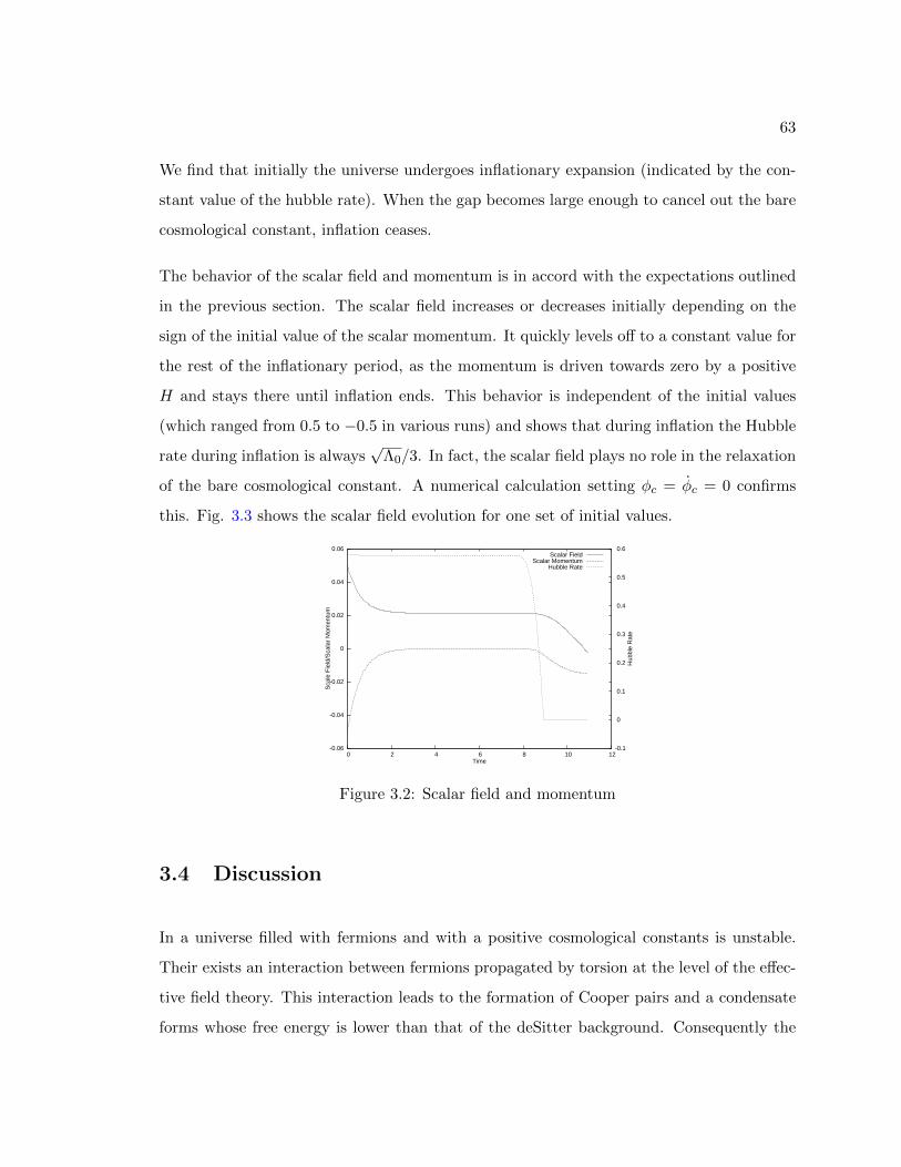
63
We find that initially the universe undergoes inflationary expansion (indicated by the con-
stant value of the hubble rate). When the gap becomes large enough to cancel out the bare
cosmological constant, inflation ceases.
The behavior of the scalar field and momentum is in accord with the expectations outlined
in the previous section. The scalar field increases or decreases initially depending on the
sign of the initial value of the scalar momentum. It quickly levels off to a constant value for
the rest of the inflationary period, as the momentum is driven towards zero by a positive
H and stays there until inflation ends. This behavior is independent of the initial values
(which ranged from 0.5 to −0.5 in various runs) and shows that during inflation the Hubble
rate during inflation is always√
Λ0/3. In fact, the scalar field plays no role in the relaxation
of the bare cosmological constant. A numerical calculation setting φc = φc = 0 confirms
this. Fig. 3.3 shows the scalar field evolution for one set of initial values.
-0.06
-0.04
-0.02
0
0.02
0.04
0.06
0 2 4 6 8 10 12-0.1
0
0.1
0.2
0.3
0.4
0.5
0.6
Sca
le F
ield
/Sca
lar
Mom
entu
m
Hub
ble
Rat
e
Time
Scalar FieldScalar Momentum
Hubble Rate
Figure 3.2: Scalar field and momentum
3.4 Discussion
In a universe filled with fermions and with a positive cosmological constants is unstable.
Their exists an interaction between fermions propagated by torsion at the level of the effec-
tive field theory. This interaction leads to the formation of Cooper pairs and a condensate
forms whose free energy is lower than that of the deSitter background. Consequently the

64
bare cosmological constant, which we identify to be the free energy of the deSitter back-
ground, is lowered by an amount proportional to the square of the condensate gap. We
have cosmic expansion because initially the gap does not cancel out the bare cosmological
constant completely. The size of the gap depends on the 3-volume. Hence as the expansion
occurs the effective cosmological ”constant” becomes smaller, until eventually after a period
of inflation we emerge from the deSitter vacuum into flat Minkowski space, where H ∼ 0.
The number of e-foldings during inflation is given by (3.15) and can be tuned by adjusting
ED and kf . The behavior of the scale factor is also independent of the scalar field evolution.
There are three free parameters in our model. The bare cosmological constant Λ0, the fermi
energy kf and the Debye energy ED. In a condensate ED is the cutoff frequency and is
determined by the lattice size. In a cosmological context therefore we can speculate that
it should be ∼ Mpl. kf can constrained according to (3.15) to be ∼ e−90. Λ0 determines
the Hubble rate during inflation. From the WMAP data [43], the upper limit on H/M2pl
is constrained to be 10−4. From this we can deduce that the bare cosmological constant,
needs to be fixed by hand to be Λ ∼ H2 ∼ 10−8M4pl in order to conform to observations.
We have presented here a non-perturbative mechanism which relaxes the bare cosmological
constant to zero. As a bonus we find that the relaxation is accompanied by an inflationary
period. The duration of inflation is determined by two parameters (ED and kf ) whose
precise determination requires physics beyond the standard model. The lack of fine-tuning
is demonstrated by the fact that the solution has an attractor with H = 0 independent of
the values of the free parameters.
The scalar field discussed here is an emergent degree of freedom. After inflation, oscillations
of this field can lead to reheating. However, to what extent this would be a viable description
of the post-inflationary period remains to be seen in future work.

Chapter 4
Cosmological Acceleration
and the Dark Energy Problem
4.1 Introduction
It is important for researchers in dark energy, and cosmology in general, to be familiar
with the observational basis for claims regarding the most appropriate cosmological model.
Perhaps the weakest link in the chain of observation and reasoning leading to the LCDM
model, lies in the assumptions used to determine luminosity distances between Earth and
the various astronomical objects that serve as “standard candles”. These calculations are
commonly done with the assumption of large-scale homogeneity in the visible universe.
Recent evidence ([53, 1, 36]) highlighting the complexity in the large-scale structure ([51,
50, 40]), conclusively demonstrates that we live in a universe whose evolution during the
current epoch cannot be described by linear perturbation theory. Such an approach is
applicable from the time of the last scattering surface (trec) upto the earliest stages of
star and galaxy formation (tstruct). Past that stage, regions with a large enough density
contrast have formed whose further evolution requires non-linear methods along the lines of
those used to describe dark matter halo evolution ([26]) . Once regions with large enough
65
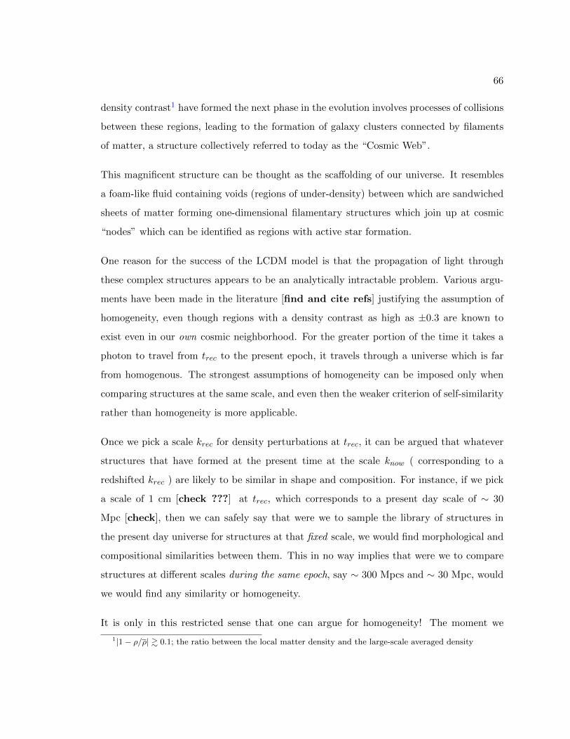
66
density contrast1 have formed the next phase in the evolution involves processes of collisions
between these regions, leading to the formation of galaxy clusters connected by filaments
of matter, a structure collectively referred to today as the “Cosmic Web”.
This magnificent structure can be thought as the scaffolding of our universe. It resembles
a foam-like fluid containing voids (regions of under-density) between which are sandwiched
sheets of matter forming one-dimensional filamentary structures which join up at cosmic
“nodes” which can be identified as regions with active star formation.
One reason for the success of the LCDM model is that the propagation of light through
these complex structures appears to be an analytically intractable problem. Various argu-
ments have been made in the literature [find and cite refs] justifying the assumption of
homogeneity, even though regions with a density contrast as high as ±0.3 are known to
exist even in our own cosmic neighborhood. For the greater portion of the time it takes a
photon to travel from trec to the present epoch, it travels through a universe which is far
from homogenous. The strongest assumptions of homogeneity can be imposed only when
comparing structures at the same scale, and even then the weaker criterion of self-similarity
rather than homogeneity is more applicable.
Once we pick a scale krec for density perturbations at trec, it can be argued that whatever
structures that have formed at the present time at the scale know ( corresponding to a
redshifted krec ) are likely to be similar in shape and composition. For instance, if we pick
a scale of 1 cm [check ???] at trec, which corresponds to a present day scale of ∼ 30
Mpc [check], then we can safely say that were we to sample the library of structures in
the present day universe for structures at that fixed scale, we would find morphological and
compositional similarities between them. This in no way implies that were we to compare
structures at different scales during the same epoch, say ∼ 300 Mpcs and ∼ 30 Mpc, would
we would find any similarity or homogeneity.
It is only in this restricted sense that one can argue for homogeneity! The moment we
1|1− ρ/ρ| & 0.1; the ratio between the local matter density and the large-scale averaged density

67
consider comparing structure at different scales we are bound to run into trouble, because
the cosmos is not scale-invariant. When considering the propogation of a photon from the
time of recombination until today it passes through many structures of very different scales
at different epochs, whose structure and composition becomes more sharply defined as we
reach closer to the present epoch. Therefore, in the absence of an investigation into the
effects of inhomogeneities on luminosity distances, the LCDM model remains standing as
the best model we have as opposed to the best model which can be determined by the
complete range of cosmological observations.
Therefore, it is fortunate that a number of such investigations have been initiated. These
include work done by Celerier [19], Inoue and Silk [29, 30] and Biswas, Mansouri, and
Notari [13] among others. In most cases, in lieu of an analytical handle on inhomogeneities
along the entire history of the photon, one generally considers an approximation where
the local patch of the cosmos, which includes our Milky Way, is described by a region of
relative under-density. This “local void” is surrounded by sheets of matter on its boundary
parts of which could conceivably be identified with the structure known as the “Great
Wall” in the SDSS. Such a geometry, consisting of a under-density void bounded by a shell
of matter embedded in a larger FRW background, can be analytically described by the
Lemaitre-Tolman-Bondi (LTB) metric. This is a first step in the direction of a complete
non-perturbative treatment.
The outline of the rest of this chapters is as follows. In Section 4.2 we describe the method
for determining cosmological distance scales using so-called “standard candles”. Section 4.3
summarizes the present evidence for “dark energy” and points out the crucial role played
by the methodology used to determine luminosity distances between objects in determining
the observed value of the cosmological constant Λobs. Section 4.4 describes cosmological
parameter estimation - for both, homogeneous and inhomogeneous cosmologies - via Markov
Chain Monte Carlo (MCMC) methods. The LTB metric is explained in Section 4.5. In
section 4.6 we compare power spectra and cosmological parameter values (for homogeneous
and inhomogeneous cosmologies) obtained by applying MCMC methods to WMAP data.

68
4.2 Cosmic Candles and Luminosity Distance
The fundamental piece of the cosmological puzzle lies in the methods available to and
employed by astronomers in order to determine distances between various cosmological
objects. Indeed, we can determine the large scale structure of the gravitational metric gµν in
a given region of spacetime with N identifiable, non-trivial sources of gravity by determining
observationally the “distance” between pairs (i, j) of such sources dij ; {i, j ∈ 1, . . . , N} . . .
show how the metric in interior of a simplex is determined given the bound-
ary data which include the lengths of edges, the area of faces and the dihedral
angle between pairs of faces.
4.3 Evidence for “dark energy”
4.4 Parameter Estimation using Markov Chain Monte Carlo
(MCMC)
Large sample space Statistical method of finding a solution Bayesian analysis =¿ Estimating
parameters given a theory and a data set Markov Chain =¿ Particular method used Software
=¿ CosmoMC by Sarah Bridle and Antony Lewis Dataset =¿ WMAP ver. 3 Hardware =¿
On PSU HPC cluster (lionxl)
4.5 LTB Model
4.6 Comparison with LCDM model
Likelihood tables

69
4.7 Discussion
There has been no lack of criticism of this model of apparent cosmic acceleration, much
of which centers around the notion that our location near the center of a large void is in
conflict with the cosmological principle and with precision cosmological measurements. For
instance the abstract of one such rebuttal [33] begins with the statement that
”The suggestion that we occupy a privileged position near the centre of a large, nonlinear,
and nearly spherical void has recently attracted much attention as an alternative to dark
energy. ....”
In this and similar rebuttals the issue of our “privileged position” near the center of a void
is often raised as a philosophical objection to the model. However, contrary to common
opinion, our location in the interior region of a void is not only likely but also necessary
from an anthropic point of view. In fact, one can go on to argue that life-bearing systems
are far more likely to occur in the relatively quiet interiors of voids rather than in the
filaments or nodes of the cosmic web which are regions of star formation and hence full of
highly energetic debris which would make the uninterrupted evolution of life on a planet
over many eons unlikely.
Such an argument is amenable to experimental confirmation or rejection by looking at the
results of the various exoplanetary searches in progress. In addition the results of void-finder
models [20] consistently show that the basic results of the various methods agree very well
with each other in that they all locate a major void near the centre of our volume.
Ultimately whether or not the void model rules out the existence of dark energy is not
by itself the major issue at stake here. It is irrefutable that the inhomogeneous large-
scale structure of the galactic web must figure into any complete analysis of CMB or other
cosmological data.

70
Find out how to insert chapter appendices, rather than one appendix for
the entire thesis
4.8 Microwave Background Radiation from Cosmic Anistropies
summarize derivation of CMB via boltzmann’s equation from chap. 9 of mukhanov
4.9 Hierarchical Structure Formulation
Structure formation is a highly non-linear process. It cannot be understand by the simple
linear theory of wavelengths entering the horizon at different redshifts. However, numerical
simulations are not the viable only line of attack. There exists an analytical framework
centered around Smulochowski’s work on fluctuations. The essential idea is that when
we look at the “entire universe”, the matter density distribution shows no fluctuations.
However, as we look at smaller and smaller scales, the fluctuations in the matter density δρρ
increase and become more random. This variation of the density with scale can be viewed
as a brownian walk - and this is where Smoluchowski’s work comes into play.
The fluctuation spectrum is embedded in the initial conditions - at recombination - and
depends on the inflationary model used. But essentially it can be fixed by hand, not
worrying about what form of inflation created it. This initial condition then determines
the future evolution of the matter density and halo formation. Even though the resulting
evolution is statistical, it is not indeterminate. The distribution of halos at different redshifts
depends on the fluctuation spectrum specified as part of the initial conditions.
The insights from the work on halo formation, from Press-Scheter to Sheth and Moreno,
can be summarized as follows:
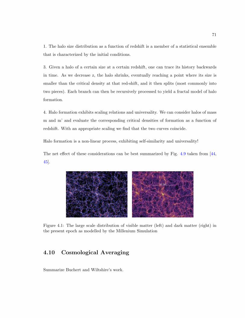
71
1. The halo size distribution as a function of redshift is a member of a statistical ensemble
that is characterized by the initial conditions.
3. Given a halo of a certain size at a certain redshift, one can trace its history backwards
in time. As we decrease z, the halo shrinks, eventually reaching a point where its size is
smaller than the critical density at that red-shift, and it then splits (most commonly into
two pieces). Each branch can then be recursively processed to yield a fractal model of halo
formation.
4. Halo formation exhibits scaling relations and universality. We can consider halos of mass
m and m’ and evaluate the corresponding critical densities of formation as a function of
redshift. With an appropriate scaling we find that the two curves coincide.
Halo formation is a non-linear process, exhibiting self-similarity and universality!
The net effect of these considerations can be best summarized by Fig. 4.9 taken from [44,
45].
Figure 4.1: The large scale distribution of visible matter (left) and dark matter (right) inthe present epoch as modelled by the Millenium Simulation
4.10 Cosmological Averaging
Summarize Buchert and Wiltshire’s work.

Bibliography
[1] Kevork N. Abazajian et al. “The Seventh Data Release of the Sloan Digital Sky Sur-vey”. In: The Astrophysical Journal Supplement Series 182.2 (June 1, 2009), pp. 543–558. issn: 0067-0049. doi: 10.1088/0067-0049/182/2/543. arXiv:0812.0649. url:http://dx.doi.org/10.1088/0067-0049/182/2/543.
[2] L. R. Abramo, N. C. Tsamis, and R. P. Woodard. “Cosmological Density Pertur-bations From A Quantum Gravitational Model Of Inflation”. In: Fortsch. Phys. 47(1999), p. 389. url: http://www.arxiv.org/astro-ph/9803172.
[3] Miguel Alcubierre. “The warp drive: hyper-fast travel within general relativity”. In:(Sept. 5, 2000). arXiv:gr- qc/0009013. url: http://arxiv.org/abs/gr- qc/
0009013.
[4] Et Al. “The Supernova Legacy Survey: Measurement of Omega M, Omega Lambdaand w from the First Year Data Set”. In: Astron. Astrophys. 447 (2006), p. 31. url:http://www.arxiv.org/astro-ph/0510447.
[5] Stephon Alexander. “A Quantum Gravitational Relaxation of The Cosmological Con-stant”. In: Phys. Lett. B 629 (2005), p. 53. url: http : / / www . citebase . org /
abstract?id=oai:arXiv.org:hep-th/0503146.
[6] Stephon Alexander, Robert Brandenberger, and Joao Magueijo. “Non-CommutativeInflation”. In: (2001). eprint: hep-th/0108190v1. url: http://arxiv.org/abs/hep-th/0108190v1.
[7] Stephon H. S. Alexander. “Inflation from D - anti-D brane annihilation”. In: Phys.Rev. D65 (2002), p. 023507. doi: 10.1103/PhysRevD.65.023507. arXiv:hep-th/0105032.
[8] Stephon H. S. Alexander and Deepak Vaid. “Gravity Induced Chiral CondensateFormation and the Cosmological Constant”. In: (Sept. 10, 2006). arXiv:hep- th/0609066. url: http://arxiv.org/abs/hep-th/0609066.
[9] Stephon Alexander, Manasse Mbonye, and John Moffat. “The Gravitational Instabil-ity of the Vacuum: Insight into the Cosmological Constant Problem”. In: (2004). url:hep-th/0406202.
72

BIBLIOGRAPHY 73
[10] Stephon Alexander and Deepak Vaid. “A fine tuning free resolution of the cosmologicalconstant problem”. In: (Feb. 8, 2007). arXiv:hep-th/0702064. url: http://arxiv.org/abs/hep-th/0702064.
[11] Nima Arkani-Hamed et al. “Ghost Inflation”. In: JCAP 0404 (2004), p. 001. url:http://www.arXiv.org/hep-th/0312100.
[12] Sundance O. Bilson-Thompson, Fotini Markopoulou, and Lee Smolin. Quantum grav-ity and the standard model. Mar. 2006. eprint: hep-th/0603022. url: http://arxiv.org/abs/hep-th/0603022.
[13] Tirthabir Biswas, Reza Mansouri, and Alessio Notari. “Nonlinear Structure Formationand ”Apparent” Acceleration: an Investigation”. In: (July 5, 2006). arXiv:astro-ph/0606703. url: http://arxiv.org/abs/astro-ph/0606703.
[14] Robert H. Brandenberger. “Back Reaction of Cosmological Perturbations and theCosmological Constant Problem”. In: (2002). url: http://www.arxiv.org/hep-th/0210165.
[15] Robert H. Brandenberger. “Principles, progress and problems in inflationary cosmol-ogy”. In: AAPPS Bull. 11 (2001), pp. 20–29. eprint: astro-ph/0208103.
[16] Robert H. Brandenberger and Ariel R. Zhitnitsky. “Can Asymptotic Series Resolvethe Problems of Inflation?” In: Phys. Rev. D 55 (1997), p. 4640. url: http://www.arXiv.org/hep-ph/9604407.
[17] Robert Brout. “Condensation of Planckian modes and the inflaton”. In: (2003).
[18] Sean M. Carroll. “The Cosmological Constant”. In: Living Rev. Rel. 4 (2001), p. 1.url: http://www.arXiv.org/astro-ph/0004075.
[19] Marie-Noelle Celerier. “Do we really see a cosmological constant in the supernovaedata ?” In: (July 11, 2007). arXiv:astro-ph/9907206. url: http://arxiv.org/abs/astro-ph/9907206.
[20] Joerg M. Colberg et al. “The Aspen-Amsterdam Void Finder Comparison Project”. In:Mon. Not. Roy. Astron. Soc. 387 (Apr. 10, 2008), pp. 933–944. doi: 10.1111/j.1365-2966.2008.13307.x. arXiv:0803.0918. url: http://dx.doi.org/10.1111/j.1365-2966.2008.13307.x.
[21] L. Crane and L. Smolin. “Space-time foam as the universal regulator”. In: GeneralRelativity and Gravitation 17 (Dec. 1985), pp. 1209–1216. doi: 10.1007/BF00773626.url: http://dx.doi.org/10.1007/BF00773626.
[22] Gia Dvali, Stefan Hofmann, and Justin Khoury. “Degravitation of the CosmologicalConstant and Graviton Width”. In: (Mar. 5, 2007). arXiv:hep-th/0703027. url:http://arxiv.org/abs/hep-th/0703027.
[23] Albert Einstein and Robert W. Lawson. Relativity: The Special and General Theory.H. Holt and Company, 1920.
[24] A. Einstein and N. Rosen. “The Particle Problem in the General Theory of Relativity”.In: Physical Review Online Archive (Prola) 48.1 (July 1935), pp. 73–77. doi: 10.1103/PhysRev.48.73. url: http://dx.doi.org/10.1103/PhysRev.48.73.

BIBLIOGRAPHY 74
[25] Alexander Fetter and John D. Walecka. Quantum theory of many-particle systems.Mineola, N.Y.: Dover, 2003. Chap. 10, p. 326.
[26] Carlo Giocoli et al. “An improved model for the formation times of dark matterhaloes”. In: (Jan. 18, 2007). arXiv:astro-ph/0611221. url: http://arxiv.org/abs/astro-ph/0611221.
[27] J. Gonzalez, F. Guinea, and M. A. H. Vozmediano. “The Electronic Spectrum ofFullerenes from the Dirac Equation”. In: (Aug. 7, 1992). doi: 10 . 1016 / 0550 -
3213(93)90009- E. arXiv:cond- mat/9208004. url: http://dx.doi.org/10.
1016/0550-3213(93)90009-E.
[28] Edwin Hubble. “A Relation between Distance and Radial Velocity among Extra-Galactic Nebulae”. In: Proceedings of the National Academy of Sciences of the UnitedStates of America 15.3 (1929), pp. 168–173.
[29] Kaiki T. Inoue and Joseph Silk. “Local Voids as the Origin of Large-angle CosmicMicrowave Background Anomalies I”. In: (Sept. 1, 2006). arXiv:astro-ph/0602478.url: http://arxiv.org/abs/astro-ph/0602478.
[30] Kaiki T. Inoue and Joseph Silk. “Local Voids as the Origin of Large-angle Cosmic Mi-crowave Background Anomalies: The Effect of a Cosmological Constant”. In: (May 20,2007). arXiv:astro-ph/0612347. url: http://arxiv.org/abs/astro-ph/0612347.
[31] Justin Khoury et al. “Ekpyrotic universe: Colliding branes and the origin of the hotbig bang”. In: 64.12 (2001), p. 123522. doi: 10.1103/PhysRevD.64.123522.
[32] Michael S. Morris and Kip S. Thorne. “Wormholes in spacetime and their use for inter-stellar travel: A tool for teaching general relativity”. In: American Journal of Physics56.5 (1988), pp. 395–412. url: http://scitation.aip.org/getabs/servlet/
GetabsServlet?prog=normal\&id=AJPIAS000056000005000395000001\&idtype=
cvips\&gifs=yes.
[33] Adam Moss, James P. Zibin, and Douglas Scott. “Precision Cosmology Defeats VoidModels for Acceleration”. In: (July 21, 2010). arXiv:1007.3725. url: http://arxiv.org/abs/1007.3725.
[34] A. H. Castro Neto et al. “The electronic properties of graphene”. In: Reviews ofModern Physics 81.1 (Feb. 29, 2008), pp. 109–162. doi: 10.1103/RevModPhys.81.109. arXiv:0709.1163. url: http://dx.doi.org/10.1103/RevModPhys.81.109.
[35] Arno A. Penzias and Robert Woodrow Wilson. “A Measurement of excess antennatemperature at 4080- Mc/s”. In: Astrophys. J. 142 (1965), pp. 419–421. doi: 10.1086/148307.
[36] Will J. Percival et al. “The 2dF Galaxy Redshift Survey: The power spectrum andthe matter content of the universe”. In: (May 15, 2001). arXiv:astro-ph/0105252.url: http://arxiv.org/abs/astro-ph/0105252.
[37] Alejandro Perez and Carlo Rovelli. “Physical effects of the Immirzi parameter inloop quantum gravity”. In: Physical Review D 73.4, 044013 (2006), p. 044013. url:http://link.aps.org/abstract/PRD/v73/e044013.

BIBLIOGRAPHY 75
[38] Tomislav Prokopec. A solution to the cosmological constant problem. 2006. url: http://www.arXiv.org/gr-qc/0603088.
[39] Gordon W. Semenoff. “Condensed-Matter Simulation of a Three-Dimensional Anomaly”.In: Physical Review Letters 53.26 (Dec. 24, 1984), pp. 2449–2452. doi: 10.1103/
PhysRevLett.53.2449. url: http://dx.doi.org/10.1103/PhysRevLett.53.2449.
[40] S. F. Shandarin, J. V. Sheth, and V. Sahni. “Morphology of the supercluster-void net-work in LCDM cosmology”. In: MON.NOT.ROY.ASTRON.SOC. 353 (2004), p. 162.eprint: astro-ph/0312110.
[41] Lee Smolin. “Linking topological quantum field theory and nonperturbative quan-tum gravity”. In: Journal of Mathematical Physics 36.11 (1995), pp. 6417–6455. url:http://scitation.aip.org/getabs/servlet/GetabsServlet?prog=normal\&id=
JMAPAQ000036000011006417000001\&idtype=cvips\&gifs=yes.
[42] Lee Smolin. “Quantum gravity with a positive cosmological constant”. In: (Sept.2002). eprint: hep-th/0209079. url: http://arxiv.org/abs/hep-th/0209079.
[43] D. N. Spergel. “Wilkinson Microwave Anisotropy Probe (WMAP) Three Year Results:Implications for Cosmology”. In: (2006). url: http://www.arxiv.org/astro-
ph/0603449.
[44] Volker Springel, Carlos S. Frenk, and Simon D. M. White. “The large-scale structureof the Universe”. In: (Apr. 27, 2006). arXiv:astro-ph/0604561. url: http://arxiv.org/abs/astro-ph/0604561.
[45] Volker Springel et al. “Simulating the joint evolution of quasars, galaxies and theirlarge-scale distribution”. In: Nature 435.7042 (Apr. 6, 2005), pp. 629–636. issn: 0028-0836. doi: 10.1038/nature03597. arXiv:astro-ph/0504097. url: http://dx.doi.org/10.1038/nature03597.
[46] T. Thiemann. “Quantum spin dynamics (QSD): V. Quantum gravity as the naturalregulator of the Hamiltonian constraint of matter quantum field theories”. In: Classicaland Quantum Gravity 15.5 (1998), pp. 1281–1314. doi: 10.1088/0264-9381/15/5/012. url: http://dx.doi.org/10.1088/0264-9381/15/5/012.
[47] Matt Visser. Lorentzian Wormholes: From Einstein to Hawking (AIP Series in Com-putational and Applied Mathematical Physics). American Institute of Physics, Aug. 9,1996. isbn: 1563966530. url: http://www.worldcat.org/isbn/1563966530.
[48] G. E. Volovik. “The Universe in a helium droplet”. In: Int. Ser. Monogr. Phys. 117(2006), pp. 1–526.
[49] Robert M. Wald. General Relativity. The University of Chicago Press, 1984.
[50] Rien van de Weygaert, Ravi Sheth, and Erwin Platen. “A hierarchy of voids”. In:Proceedings of the International Astronomical Union 2004.IAUC195 (Apr. 20, 2004),pp. 58–63. doi: 10.1017/S1743921304000134. arXiv:astro-ph/0404397. url: http://dx.doi.org/10.1017/S1743921304000134.

BIBLIOGRAPHY 76
[51] Rien van de Weygaert et al. “Geometry and Morphology of the Cosmic Web: Ana-lyzing Spatial Patterns in the Universe”. In: (Dec. 17, 2009). arXiv:0912.3448. url:http://arxiv.org/abs/0912.3448.
[52] Wikipedia. Cosmology — Wikipedia, The Free Encyclopedia. 2008.
[53] Donald G. York et al. “The Sloan Digital Sky Survey: Technical Summary”. In: TheAstronomical Journal 120 (Sept. 1, 2000), pp. 1579–1587. doi: 10.1086/301513.arXiv:astro-ph/0006396. url: http://dx.doi.org/10.1086/301513.

Deepak Vaid
A-16, 1st Floor (East Facing)South Extension, Part IINew Delhi - 110049India
Phone: +91-11-65363116 (Landline)+91-9717275953 (Cell)
Email: [email protected]
Homepage: Link
Personal
• Citizen of India
• B.S. Physics, University of Missouri at Rolla2, 2000–2003
• Ph.D. Physics, Pennsylvania State University, 2003–2011, (defended Nov. 2010, grad-uation May, 2012)
Publications
• Gravity Induced Chiral Condensate Formation and the Cosmological Constant (with.S. Alexander), 2006, arXiv:hep-th/0609066
• A fine tuning free resolution of the cosmological constant problem (with S. Alexander),2007, arXiv:hep-th/0702064
• Local Void vs Dark Energy: Confrontation with WMAP and Type Ia Supernovae(with S. Alexander, T. Biswas and A. Notari), 2008, arXiv:abs/0712.0370
• Embedding the Bilson-Thompson model in an LQG-like framework, 2010, arXiv:abs/1002.1462
References
• Sundance Bilson-Thompson, Ramsay Postdoctoral Fellow, School of Chemistry andPhysics, University of Adelaide, [email protected]
• Jainendra K. Jain, Erwin W. Mueller Professor of Physics, Pennsylvania State Uni-versity, PA, USA, [email protected]
• Stephon Alexander, Associate Professor of Physics, Haverford College, Haverford, PA,USA, [email protected]
• Martin Bojowald, Associate Professor of Physics, Pennsylvania State University, PA,USA, [email protected]
2now known as Missouri University of Science and Technology