the cplex 12.6.x series
TRANSCRIPT
© 2016 IBM Corporation
IBM CPLEX Optimizer
The 12.6.x series, 2013-2015
Xavier Nodet, Program Manager, CPLEX Optimization [email protected]
© 2016 IBM Corporation2
Agenda
MIP Performance
Distributed MIP
Beyond Linear Programming
MISOCP
Nonconvex MIQP
Miscellaneous smaller features and new parameters
Under the hood improvements for performance
© 2016 IBM Corporation3
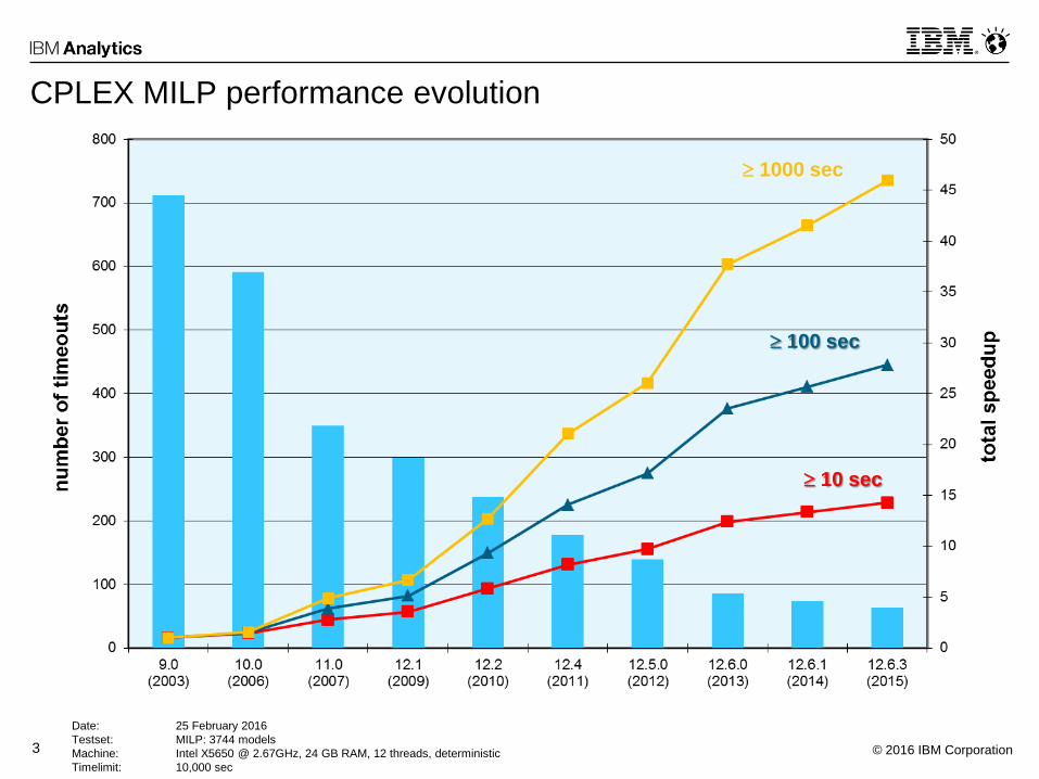
CPLEX MILP performance evolution
10 sec
100 sec
1000 sec
Date: 25 February 2016
Testset: MILP: 3744 models
Machine: Intel X5650 @ 2.67GHz, 24 GB RAM, 12 threads, deterministic
Timelimit: 10,000 sec
© 2016 IBM Corporation4
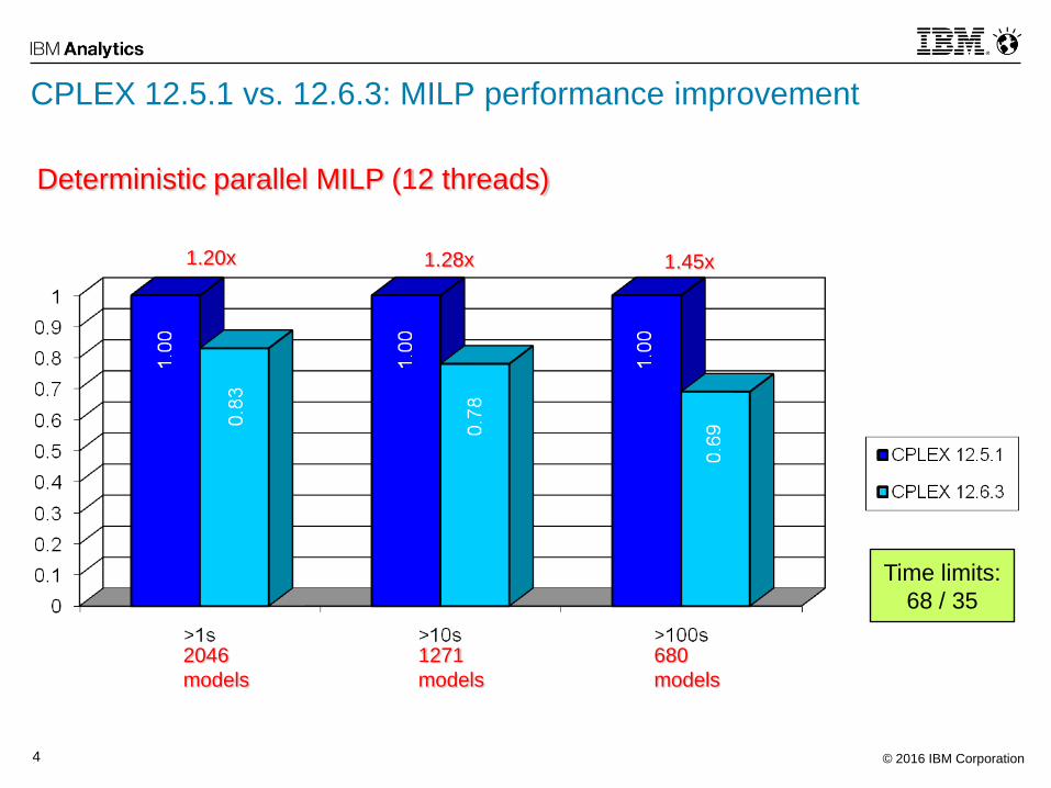
Deterministic parallel MILP (12 threads)
2046
models
1271
models
680
models
Time limits:
68 / 35
1.20x 1.28x 1.45x
CPLEX 12.5.1 vs. 12.6.3: MILP performance improvement
© 2016 IBM Corporation5
DISTRIBUTED MIP
© 2016 IBM Corporation6
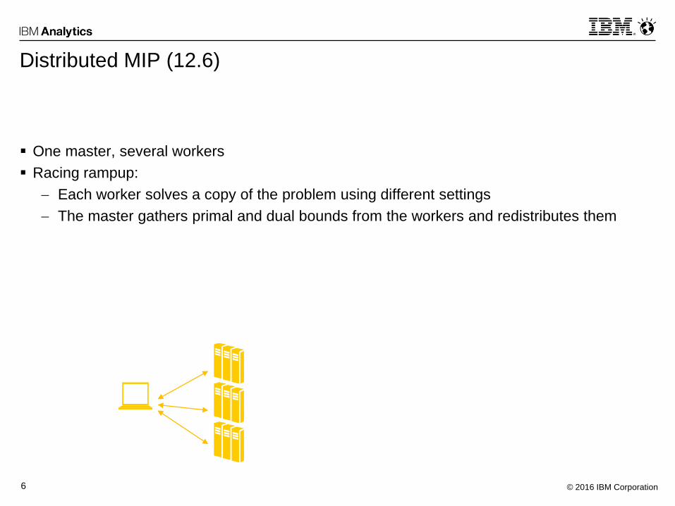
Distributed MIP (12.6)
One master, several workers
Racing rampup:
Each worker solves a copy of the problem using different settings
The master gathers primal and dual bounds from the workers and redistributes them
© 2016 IBM Corporation7
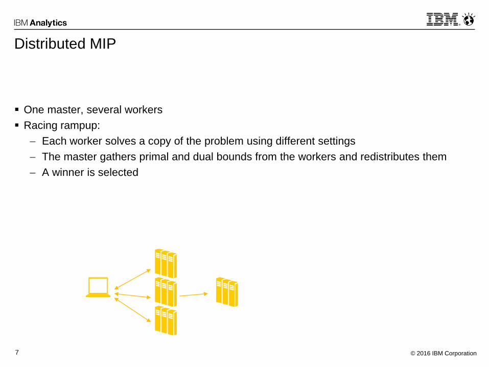
Distributed MIP
One master, several workers
Racing rampup:
Each worker solves a copy of the problem using different settings
The master gathers primal and dual bounds from the workers and redistributes them
A winner is selected
© 2016 IBM Corporation8
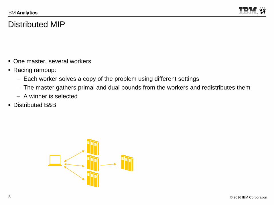
Distributed MIP
One master, several workers
Racing rampup:
Each worker solves a copy of the problem using different settings
The master gathers primal and dual bounds from the workers and redistributes them
A winner is selected
Distributed B&B
© 2016 IBM Corporation9
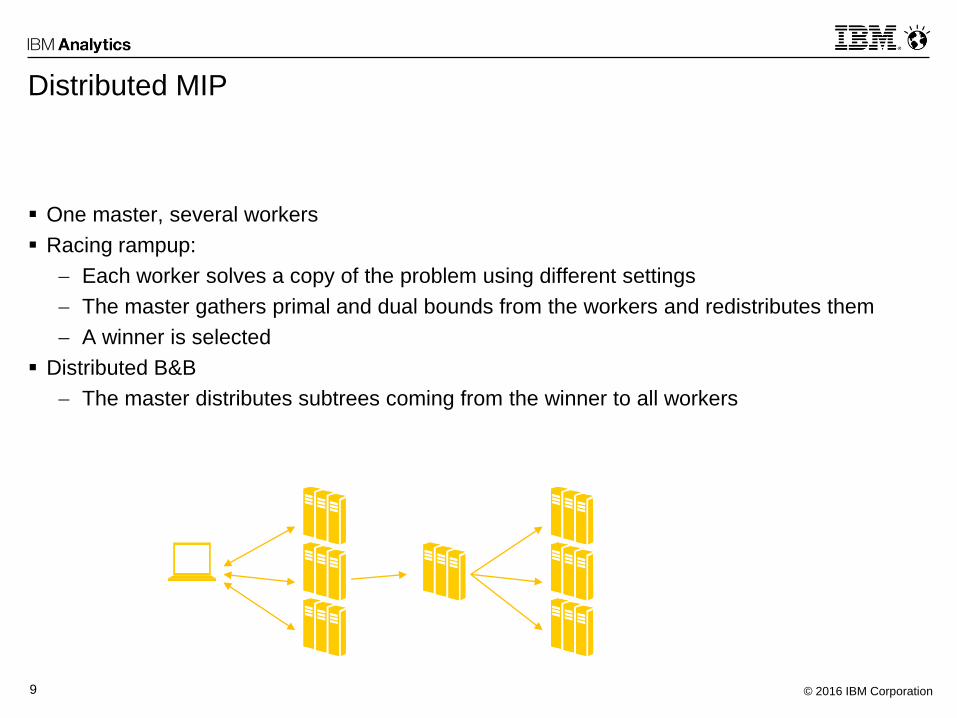
Distributed MIP
One master, several workers
Racing rampup:
Each worker solves a copy of the problem using different settings
The master gathers primal and dual bounds from the workers and redistributes them
A winner is selected
Distributed B&B
The master distributes subtrees coming from the winner to all workers
© 2016 IBM Corporation10
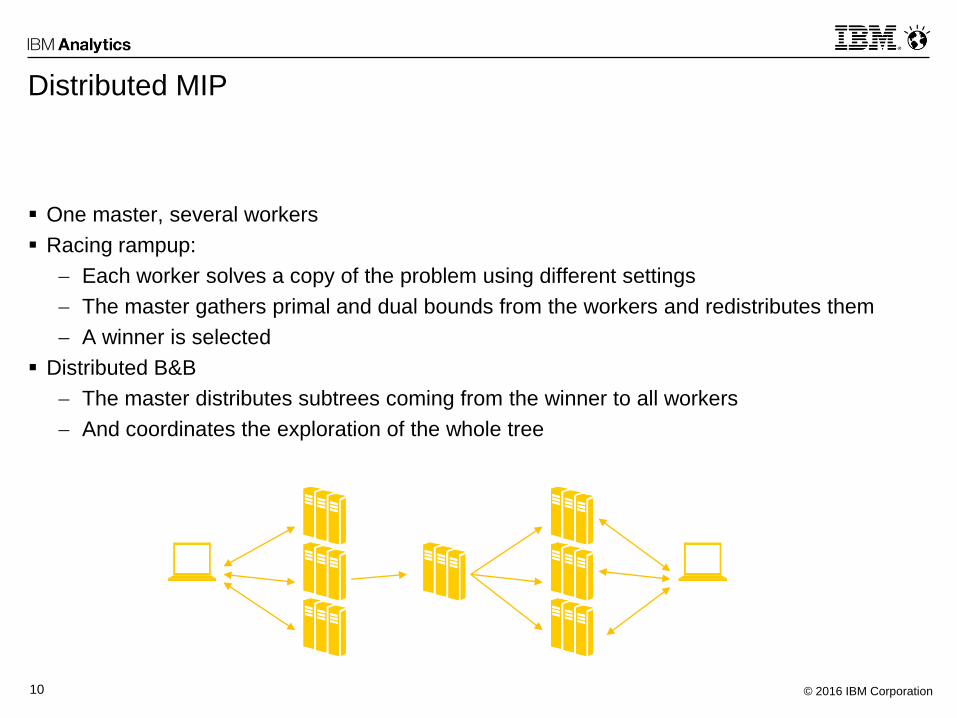
Distributed MIP
One master, several workers
Racing rampup:
Each worker solves a copy of the problem using different settings
The master gathers primal and dual bounds from the workers and redistributes them
A winner is selected
Distributed B&B
The master distributes subtrees coming from the winner to all workers
And coordinates the exploration of the whole tree
© 2016 IBM Corporation11
Distributed MIP
Use infinite rampup (default) to exploit performance variability
Use Distributed B&B
For very hard problems, many nodes to enumerate
Hardware doesn’t need to be the same
But workers should be as similar as possible to facilitate load balancing
Else Opportunistic mode should be used (‘set parallel -1’)
© 2016 IBM Corporation12
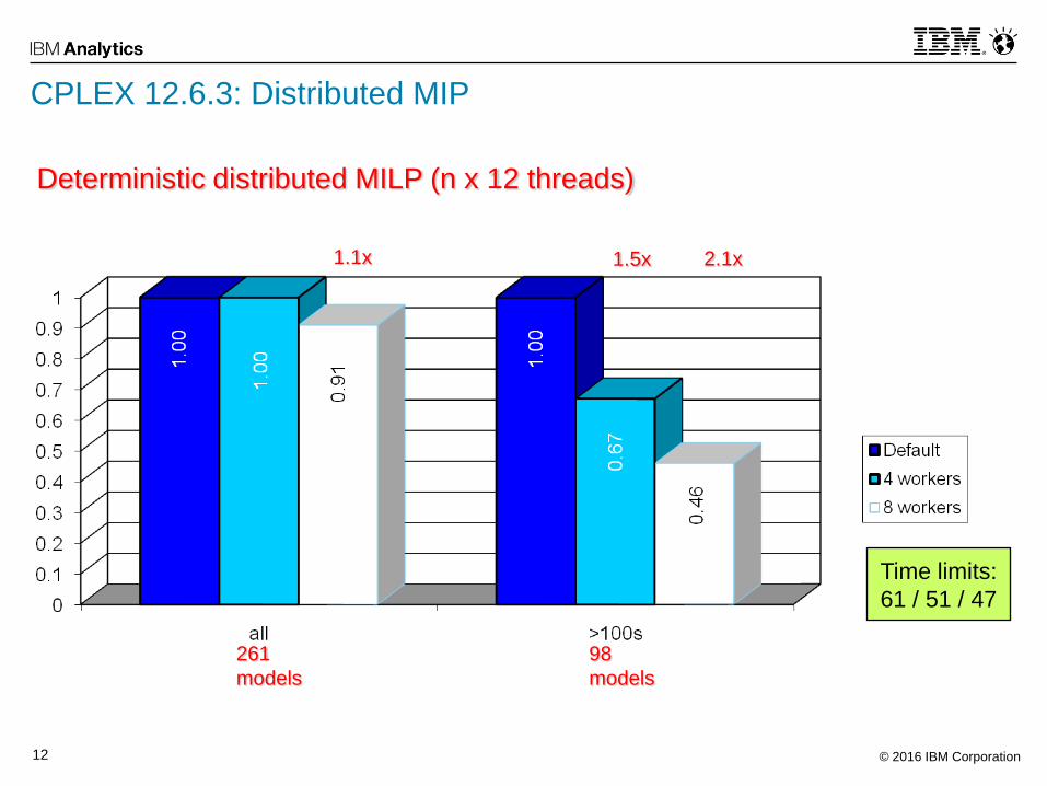
Deterministic distributed MILP (n x 12 threads)
261
models
98
models
Time limits:
61 / 51 / 47
1.1x 1.5x 2.1x
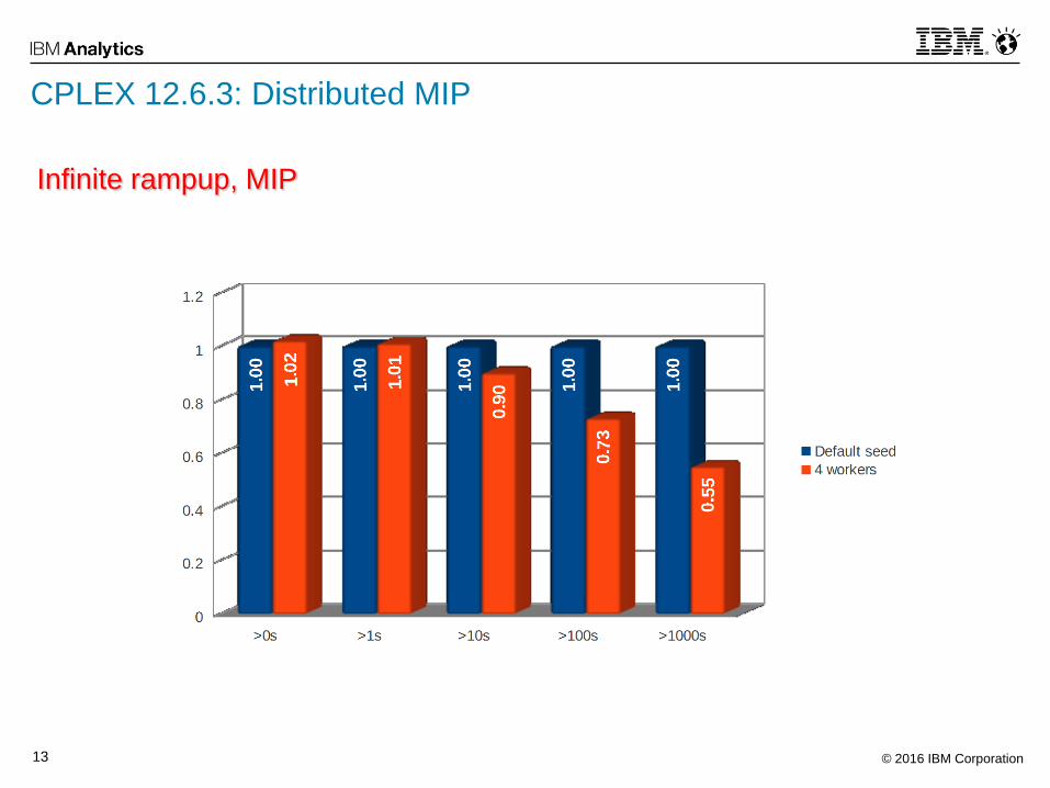
CPLEX 12.6.3: Distributed MIP
© 2016 IBM Corporation13
Infinite rampup, MIP
CPLEX 12.6.3: Distributed MIP
© 2016 IBM Corporation14
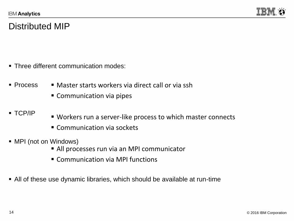
Distributed MIP
Three different communication modes:
Process
TCP/IP
MPI (not on Windows)
All of these use dynamic libraries, which should be available at run-time
Master starts workers via direct call or via ssh
Communication via pipes
Workers run a server-like process to which master connects
Communication via sockets
All processes run via an MPI communicator
Communication via MPI functions
© 2016 IBM Corporation15
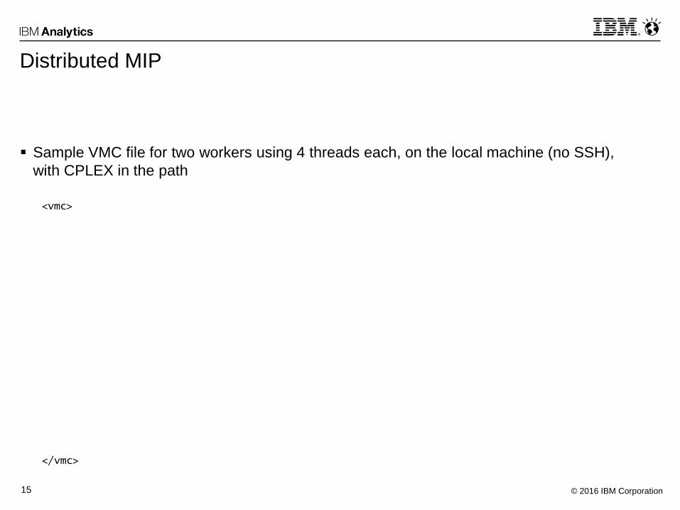
Distributed MIP
Sample VMC file for two workers using 4 threads each, on the local machine (no SSH),
with CPLEX in the path
<vmc>
</vmc>
© 2016 IBM Corporation16
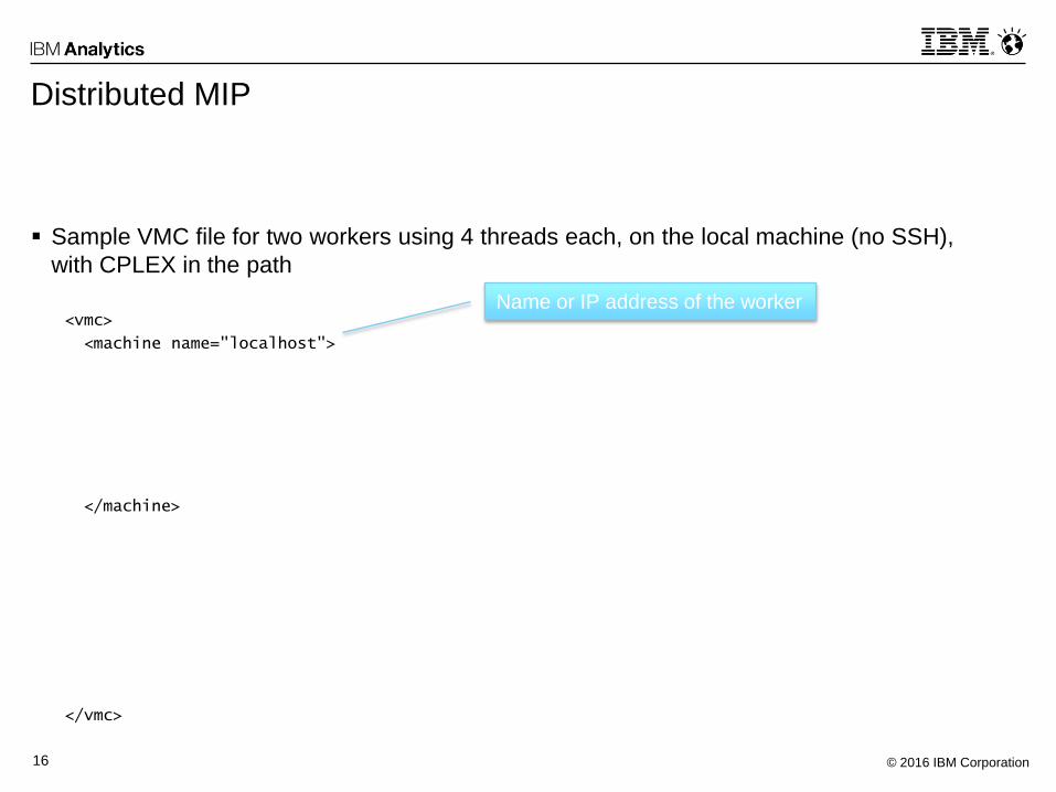
Distributed MIP
Sample VMC file for two workers using 4 threads each, on the local machine (no SSH),
with CPLEX in the path
<vmc>
<machine name="localhost">
</machine>
</vmc>
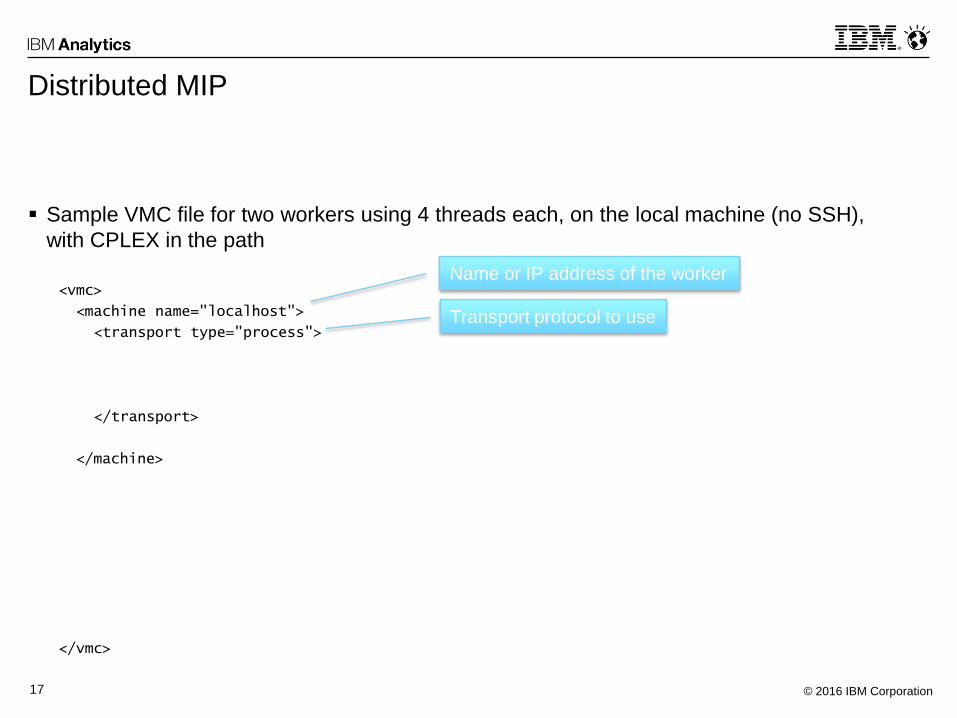
Name or IP address of the worker
© 2016 IBM Corporation17
Distributed MIP
Sample VMC file for two workers using 4 threads each, on the local machine (no SSH),
with CPLEX in the path
<vmc>
<machine name="localhost">
<transport type="process">
</transport>
</machine>
</vmc>
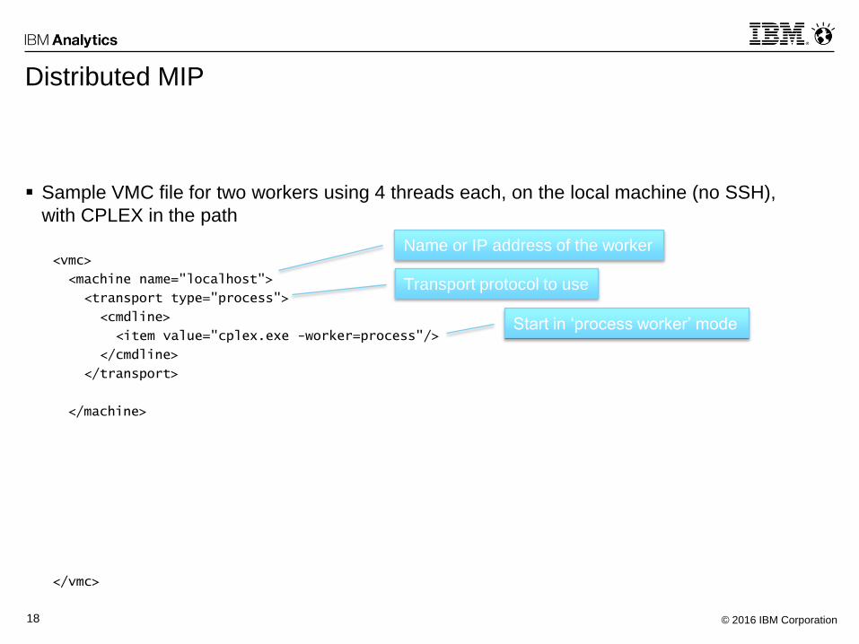
Transport protocol to use
Name or IP address of the worker
© 2016 IBM Corporation18
Distributed MIP
Sample VMC file for two workers using 4 threads each, on the local machine (no SSH),
with CPLEX in the path
<vmc>
<machine name="localhost">
<transport type="process">
<cmdline>
<item value="cplex.exe -worker=process"/>
</cmdline>
</transport>
</machine>
</vmc>
Transport protocol to use
Name or IP address of the worker
Start in ‘process worker’ mode
© 2016 IBM Corporation19
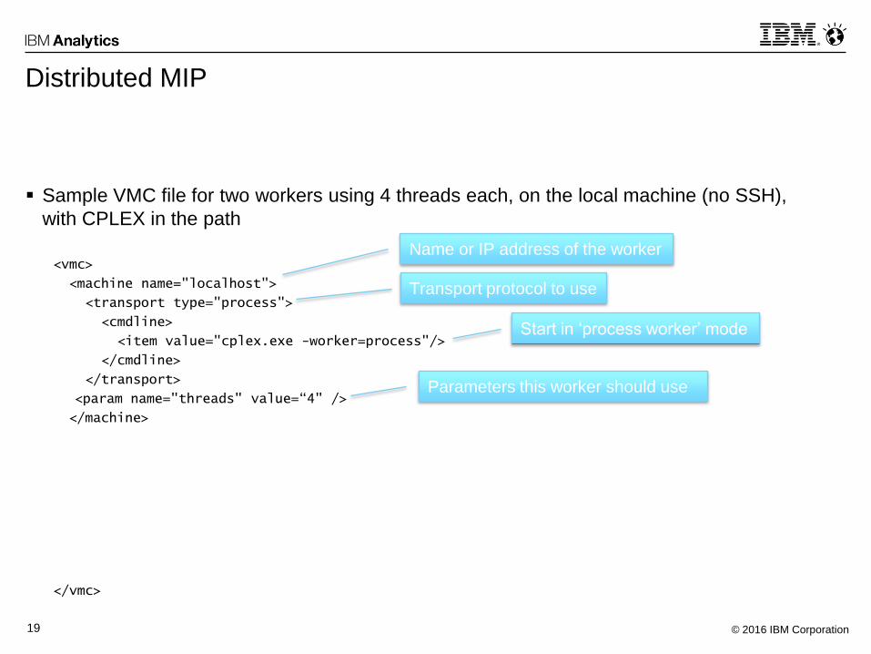
Distributed MIP
Sample VMC file for two workers using 4 threads each, on the local machine (no SSH),
with CPLEX in the path
<vmc>
<machine name="localhost">
<transport type="process">
<cmdline>
<item value="cplex.exe -worker=process"/>
</cmdline>
</transport>
<param name="threads" value=“4" />
</machine>
</vmc>
Transport protocol to use
Name or IP address of the worker
Start in ‘process worker’ mode
Parameters this worker should use
© 2016 IBM Corporation20
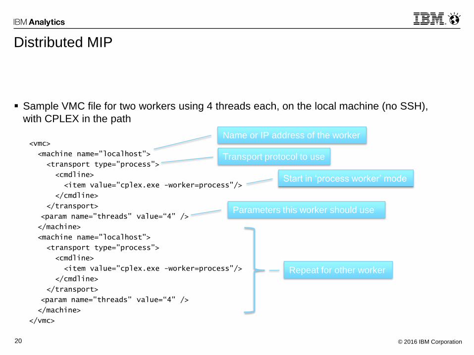
Distributed MIP
Sample VMC file for two workers using 4 threads each, on the local machine (no SSH),
with CPLEX in the path
<vmc>
<machine name="localhost">
<transport type="process">
<cmdline>
<item value="cplex.exe -worker=process"/>
</cmdline>
</transport>
<param name="threads" value=“4" />
</machine>
<machine name="localhost">
<transport type="process">
<cmdline>
<item value="cplex.exe -worker=process"/>
</cmdline>
</transport>
<param name="threads" value=“4" />
</machine>
</vmc>
Transport protocol to use
Name or IP address of the worker
Start in ‘process worker’ mode
Parameters this worker should use
Repeat for other worker
© 2016 IBM Corporation21
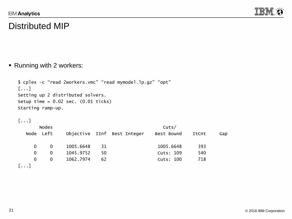
Distributed MIP
Running with 2 workers:
$ cplex –c “read 2workers.vmc” “read mymodel.lp.gz” “opt”
[...]
Setting up 2 distributed solvers.
Setup time = 0.02 sec. (0.01 ticks)
Starting ramp-up.
[...]
Nodes Cuts/
Node Left Objective IInf Best Integer Best Bound ItCnt Gap
0 0 1005.6648 31 1005.6648 393
0 0 1045.9752 50 Cuts: 109 540
0 0 1062.7974 62 Cuts: 100 718
[...]
© 2016 IBM Corporation22
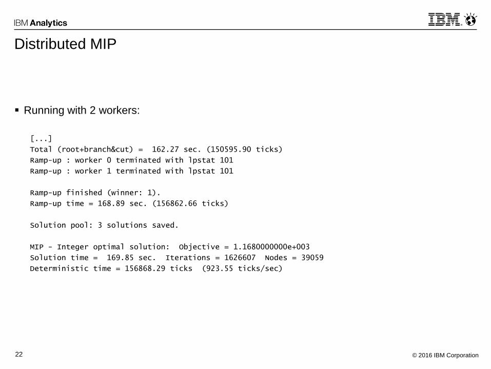
Distributed MIP
Running with 2 workers:
[...]
Total (root+branch&cut) = 162.27 sec. (150595.90 ticks)
Ramp-up : worker 0 terminated with lpstat 101
Ramp-up : worker 1 terminated with lpstat 101
Ramp-up finished (winner: 1).
Ramp-up time = 168.89 sec. (156862.66 ticks)
Solution pool: 3 solutions saved.
MIP - Integer optimal solution: Objective = 1.1680000000e+003
Solution time = 169.85 sec. Iterations = 1626607 Nodes = 39059
Deterministic time = 156868.29 ticks (923.55 ticks/sec)
© 2016 IBM Corporation23
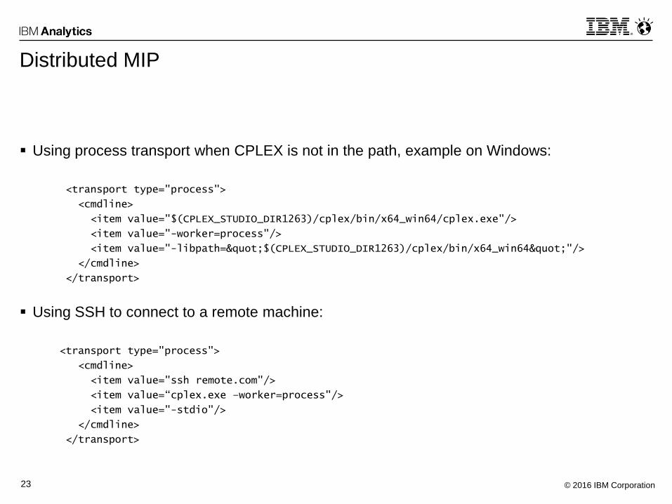
Distributed MIP
Using process transport when CPLEX is not in the path, example on Windows:
<transport type="process">
<cmdline>
<item value="$(CPLEX_STUDIO_DIR1263)/cplex/bin/x64_win64/cplex.exe"/>
<item value="-worker=process"/>
<item value="-libpath="$(CPLEX_STUDIO_DIR1263)/cplex/bin/x64_win64""/>
</cmdline>
</transport>
Using SSH to connect to a remote machine:
<transport type="process">
<cmdline>
<item value="ssh remote.com"/>
<item value=“cplex.exe –worker=process"/>
<item value="-stdio"/>
</cmdline>
</transport>
© 2016 IBM Corporation24
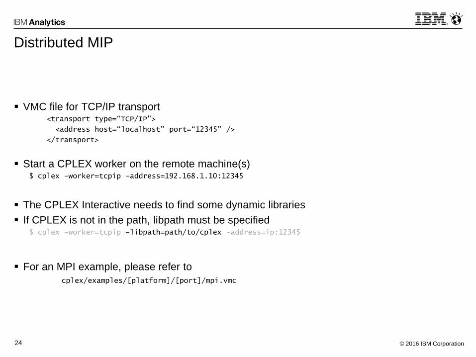
Distributed MIP
VMC file for TCP/IP transport<transport type=“TCP/IP">
<address host=“localhost” port=“12345” />
</transport>
Start a CPLEX worker on the remote machine(s)$ cplex -worker=tcpip -address=192.168.1.10:12345
The CPLEX Interactive needs to find some dynamic libraries
If CPLEX is not in the path, libpath must be specified$ cplex -worker=tcpip –libpath=path/to/cplex -address=ip:12345
For an MPI example, please refer to
cplex/examples/[platform]/[port]/mpi.vmc
© 2016 IBM Corporation25
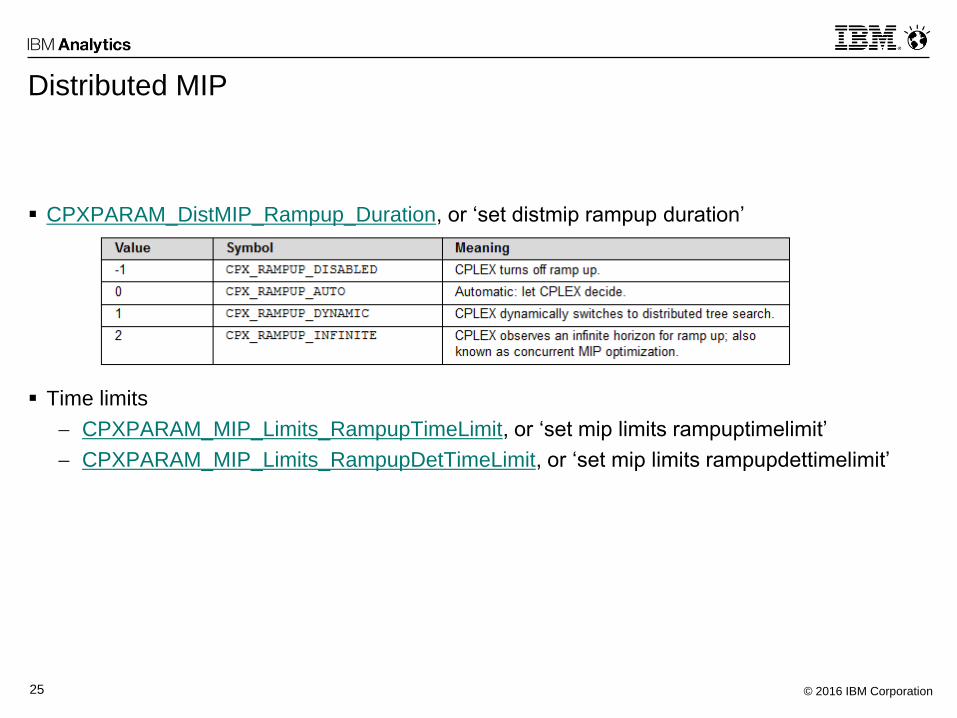
Distributed MIP
CPXPARAM_DistMIP_Rampup_Duration, or ‘set distmip rampup duration’
Time limits
CPXPARAM_MIP_Limits_RampupTimeLimit, or ‘set mip limits rampuptimelimit’
CPXPARAM_MIP_Limits_RampupDetTimeLimit, or ‘set mip limits rampupdettimelimit’
© 2016 IBM Corporation26
BEYOND LINEAR
PROGRAMMING
© 2016 IBM Corporation27
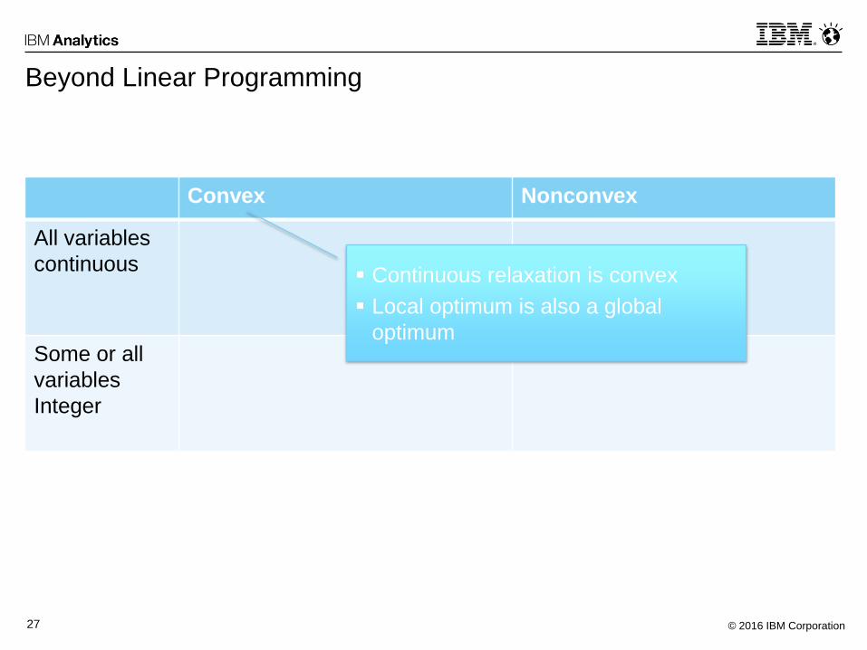
Beyond Linear Programming
Convex Nonconvex
All variables
continuous
Some or all
variables
Integer
Continuous relaxation is convex
Local optimum is also a global
optimum
© 2016 IBM Corporation28
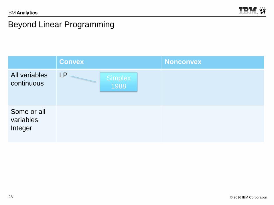
Beyond Linear Programming
Convex Nonconvex
All variables
continuous
LP
Some or all
variables
Integer
Simplex
1988
© 2016 IBM Corporation29
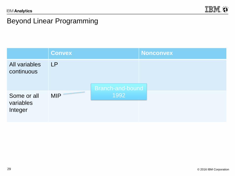
Beyond Linear Programming
Convex Nonconvex
All variables
continuous
LP
Some or all
variables
Integer
MIP
Branch-and-bound
1992
© 2016 IBM Corporation30
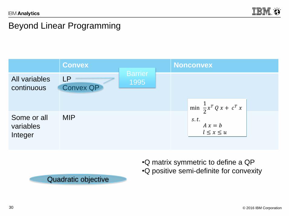
Beyond Linear Programming
Convex Nonconvex
All variables
continuous
LP
Convex QP
Some or all
variables
Integer
MIP
Quadratic objective
Barrier
1995
•Q matrix symmetric to define a QP
•Q positive semi-definite for convexity
© 2016 IBM Corporation31
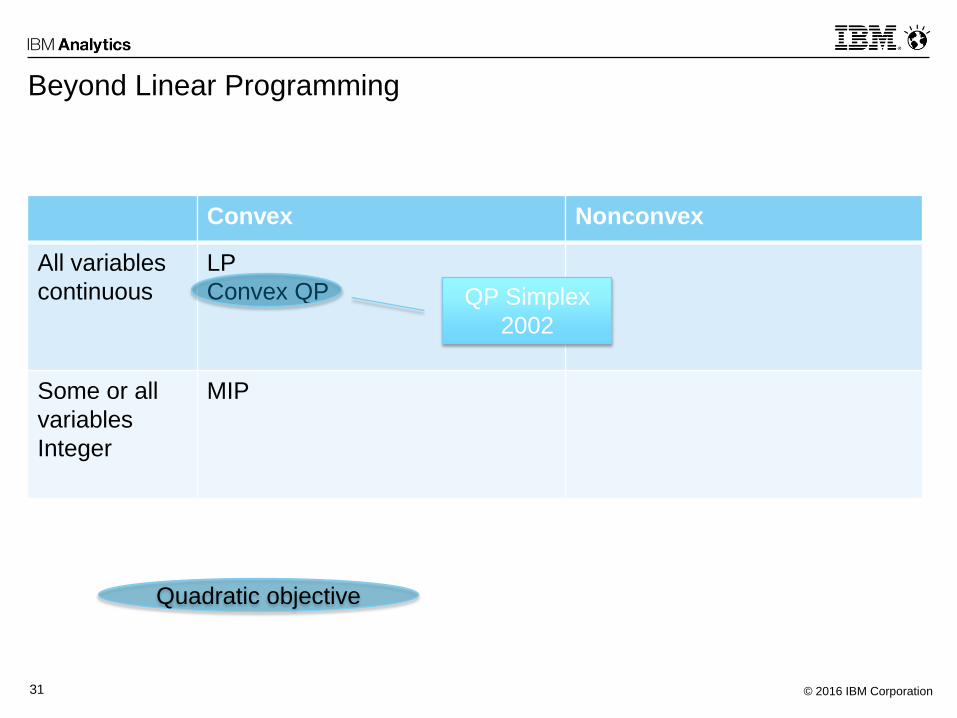
Beyond Linear Programming
Convex Nonconvex
All variables
continuous
LP
Convex QP
Some or all
variables
Integer
MIP
Quadratic objective
QP Simplex
2002
© 2016 IBM Corporation32
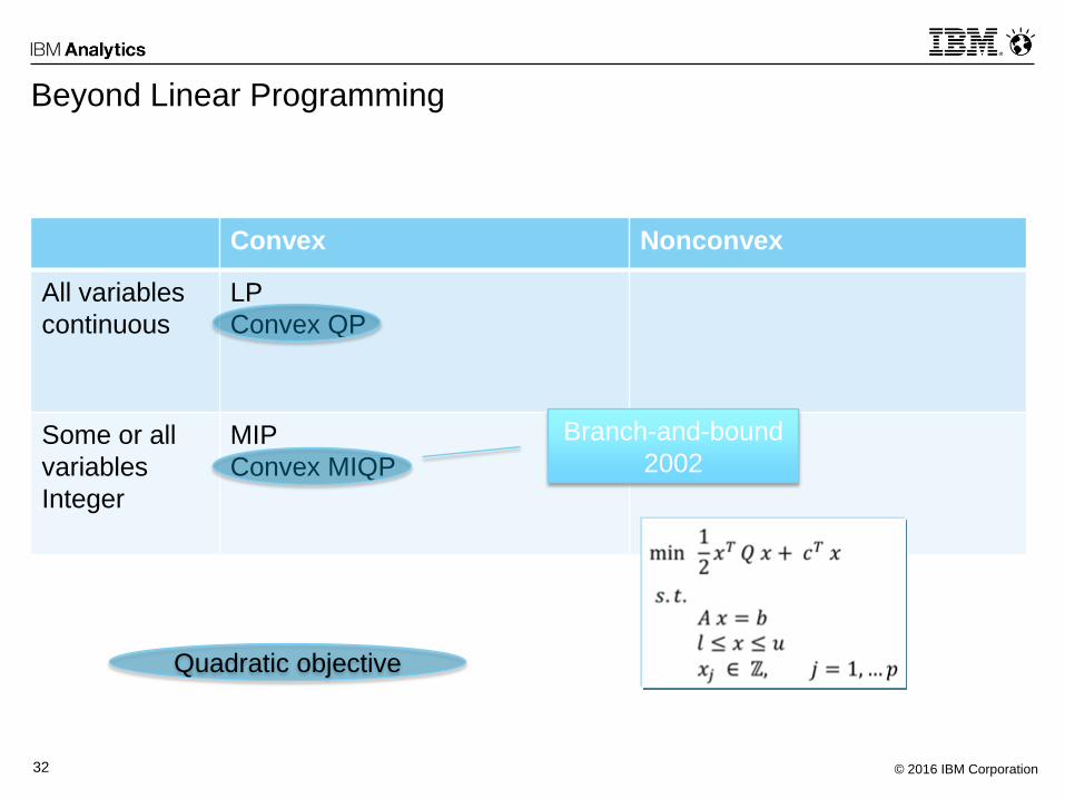
Beyond Linear Programming
Convex Nonconvex
All variables
continuous
LP
Convex QP
Some or all
variables
Integer
MIP
Convex MIQP
Quadratic objective
Branch-and-bound
2002
© 2016 IBM Corporation33
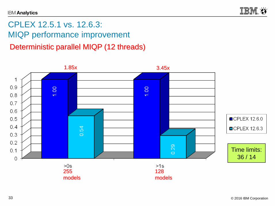
Deterministic parallel MIQP (12 threads)
255
models
128
models
Time limits:
36 / 14
1.85x 3.45x
CPLEX 12.5.1 vs. 12.6.3:
MIQP performance improvement
© 2016 IBM Corporation34
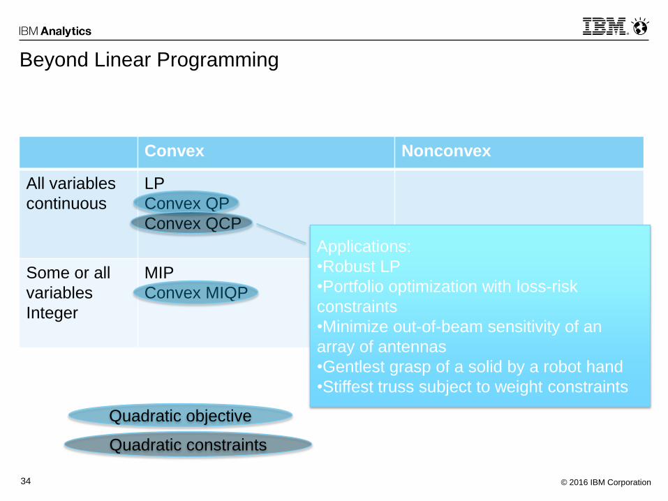
Beyond Linear Programming
Convex Nonconvex
All variables
continuous
LP
Convex QP
Convex QCP
Some or all
variables
Integer
MIP
Convex MIQP
Quadratic objective
Quadratic constraints
Applications:
•Robust LP
•Portfolio optimization with loss-risk
constraints
•Minimize out-of-beam sensitivity of an
array of antennas
•Gentlest grasp of a solid by a robot hand
•Stiffest truss subject to weight constraints
© 2016 IBM Corporation35
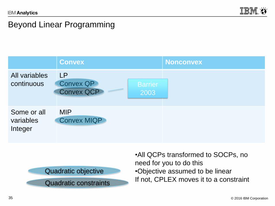
Beyond Linear Programming
Convex Nonconvex
All variables
continuous
LP
Convex QP
Convex QCP
Some or all
variables
Integer
MIP
Convex MIQP
Quadratic objective
Quadratic constraints
•All QCPs transformed to SOCPs, no
need for you to do this
•Objective assumed to be linear
If not, CPLEX moves it to a constraint
Barrier
2003
© 2016 IBM Corporation36
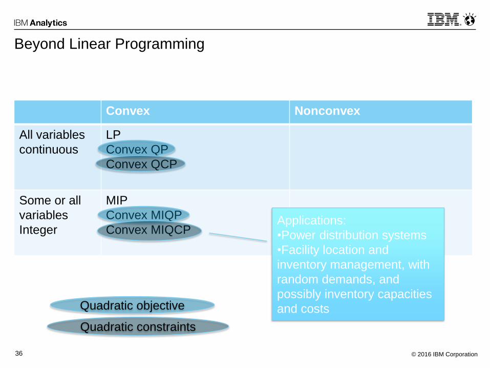
Beyond Linear Programming
Convex Nonconvex
All variables
continuous
LP
Convex QP
Convex QCP
Some or all
variables
Integer
MIP
Convex MIQP
Convex MIQCP
Quadratic objective
Quadratic constraints
Applications:
•Power distribution systems
•Facility location and
inventory management, with
random demands, and
possibly inventory capacities
and costs
© 2016 IBM Corporation37
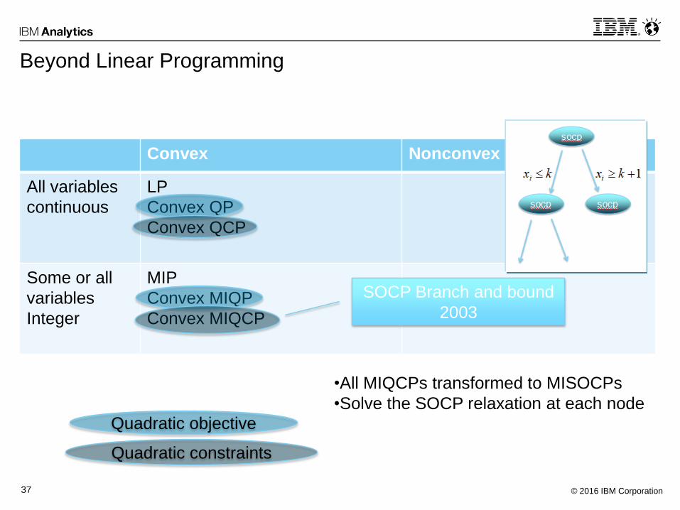
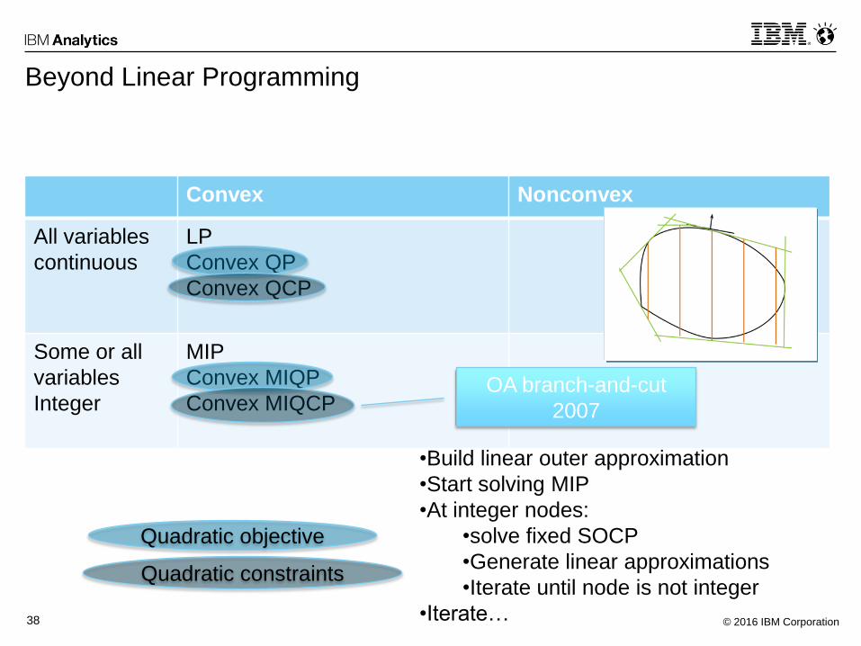
Beyond Linear Programming
Convex Nonconvex
All variables
continuous
LP
Convex QP
Convex QCP
Some or all
variables
Integer
MIP
Convex MIQP
Convex MIQCP
Quadratic objective
Quadratic constraints
•All MIQCPs transformed to MISOCPs
•Solve the SOCP relaxation at each node
SOCP Branch and bound
2003
© 2016 IBM Corporation38
Beyond Linear Programming
Convex Nonconvex
All variables
continuous
LP
Convex QP
Convex QCP
Some or all
variables
Integer
MIP
Convex MIQP
Convex MIQCP
Quadratic objective
Quadratic constraints
OA branch-and-cut
2007
•Build linear outer approximation
•Start solving MIP
•At integer nodes:
•solve fixed SOCP
•Generate linear approximations
•Iterate until node is not integer
•Iterate…
© 2016 IBM Corporation39
ALGORITHMS FOR MISOCP
© 2016 IBM Corporation40
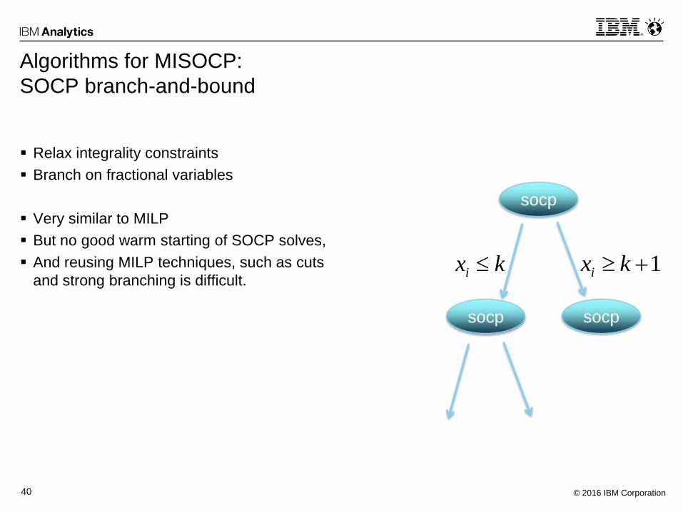
Algorithms for MISOCP:
SOCP branch-and-bound
Relax integrality constraints
Branch on fractional variables
Very similar to MILP
But no good warm starting of SOCP solves,
And reusing MILP techniques, such as cuts
and strong branching is difficult.kxi 1 kxi
socp
socp socp
© 2016 IBM Corporation41
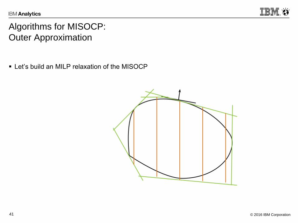
Algorithms for MISOCP:
Outer Approximation
Let’s build an MILP relaxation of the MISOCP
© 2016 IBM Corporation42
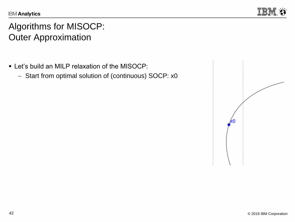
Algorithms for MISOCP:
Outer Approximation
Let’s build an MILP relaxation of the MISOCP:
Start from optimal solution of (continuous) SOCP: x0
© 2016 IBM Corporation43
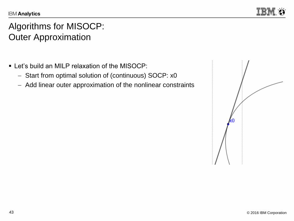
Algorithms for MISOCP:
Outer Approximation
Let’s build an MILP relaxation of the MISOCP:
Start from optimal solution of (continuous) SOCP: x0
Add linear outer approximation of the nonlinear constraints
© 2016 IBM Corporation44
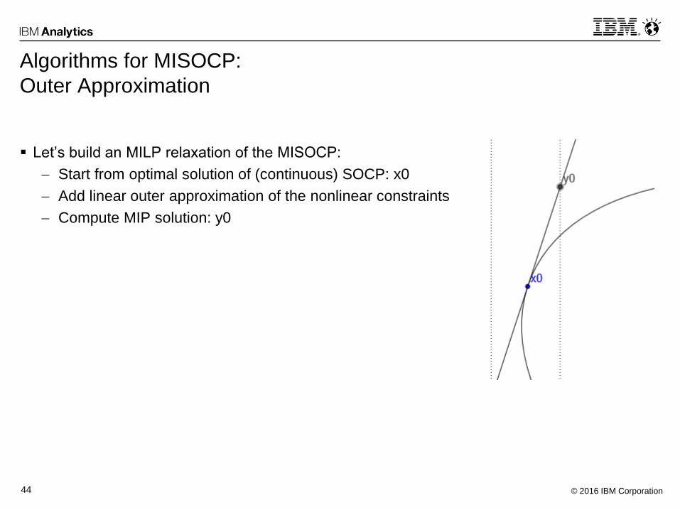
Algorithms for MISOCP:
Outer Approximation
Let’s build an MILP relaxation of the MISOCP:
Start from optimal solution of (continuous) SOCP: x0
Add linear outer approximation of the nonlinear constraints
Compute MIP solution: y0
© 2016 IBM Corporation45
Algorithms for MISOCP:
Outer Approximation
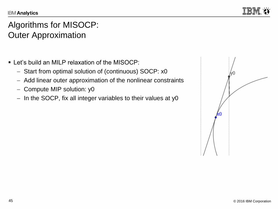
Let’s build an MILP relaxation of the MISOCP:
Start from optimal solution of (continuous) SOCP: x0
Add linear outer approximation of the nonlinear constraints
Compute MIP solution: y0
In the SOCP, fix all integer variables to their values at y0
© 2016 IBM Corporation46
Algorithms for MISOCP:
Outer Approximation
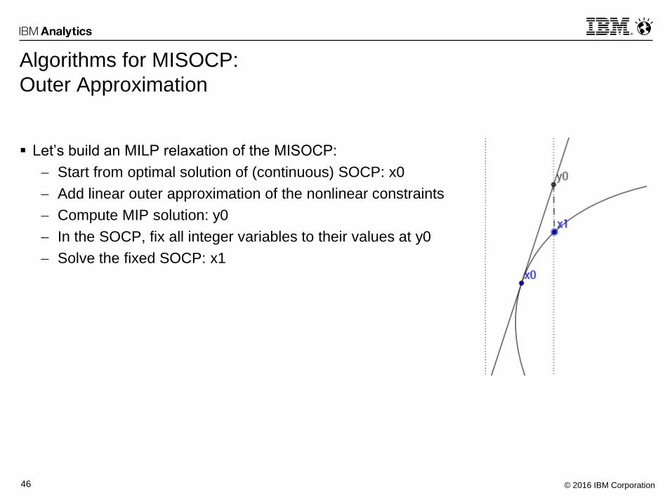
Let’s build an MILP relaxation of the MISOCP:
Start from optimal solution of (continuous) SOCP: x0
Add linear outer approximation of the nonlinear constraints
Compute MIP solution: y0
In the SOCP, fix all integer variables to their values at y0
Solve the fixed SOCP: x1
© 2016 IBM Corporation47
Algorithms for MISOCP:
Outer Approximation
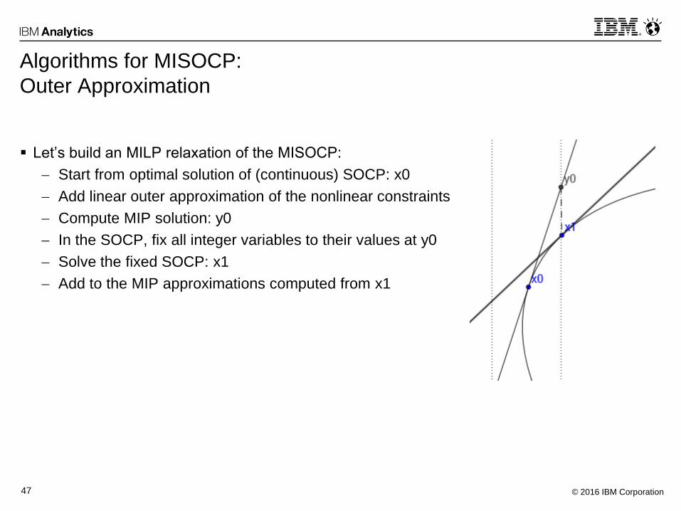
Let’s build an MILP relaxation of the MISOCP:
Start from optimal solution of (continuous) SOCP: x0
Add linear outer approximation of the nonlinear constraints
Compute MIP solution: y0
In the SOCP, fix all integer variables to their values at y0
Solve the fixed SOCP: x1
Add to the MIP approximations computed from x1
© 2016 IBM Corporation48
Algorithms for MISOCP:
Outer Approximation
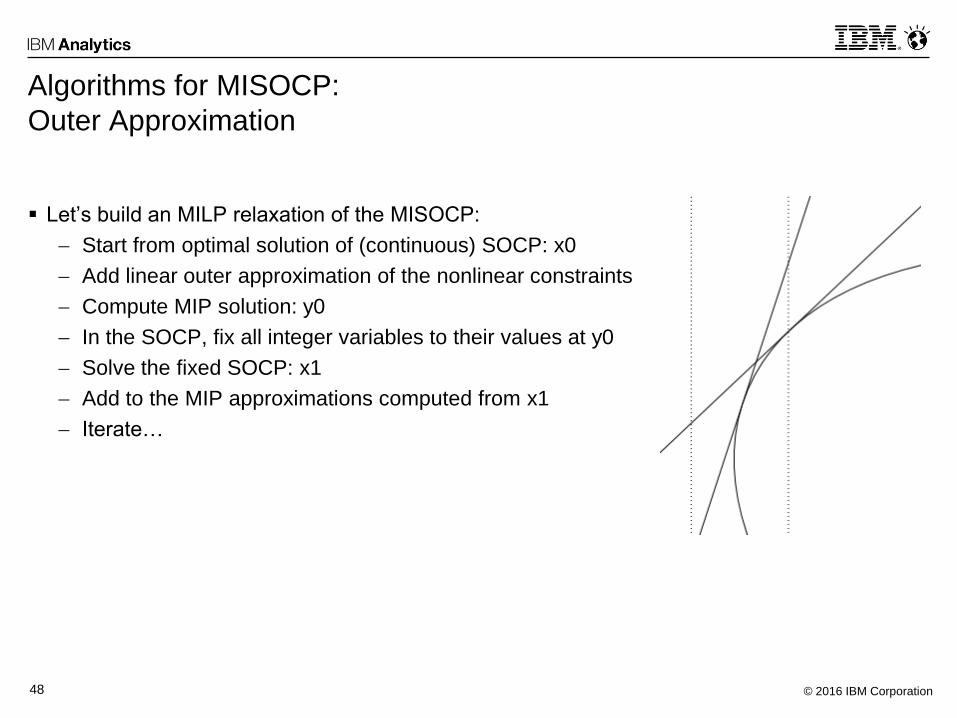
Let’s build an MILP relaxation of the MISOCP:
Start from optimal solution of (continuous) SOCP: x0
Add linear outer approximation of the nonlinear constraints
Compute MIP solution: y0
In the SOCP, fix all integer variables to their values at y0
Solve the fixed SOCP: x1
Add to the MIP approximations computed from x1
Iterate…
© 2016 IBM Corporation49
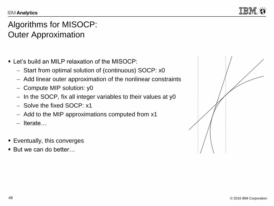
Algorithms for MISOCP:
Outer Approximation
Let’s build an MILP relaxation of the MISOCP:
Start from optimal solution of (continuous) SOCP: x0
Add linear outer approximation of the nonlinear constraints
Compute MIP solution: y0
In the SOCP, fix all integer variables to their values at y0
Solve the fixed SOCP: x1
Add to the MIP approximations computed from x1
Iterate…
Eventually, this converges
But we can do better…
© 2016 IBM Corporation50
Algorithms for MISOCP:
Outer Approximation Branch & Cut
Let’s combine OA with a MIP tree
© 2016 IBM Corporation51
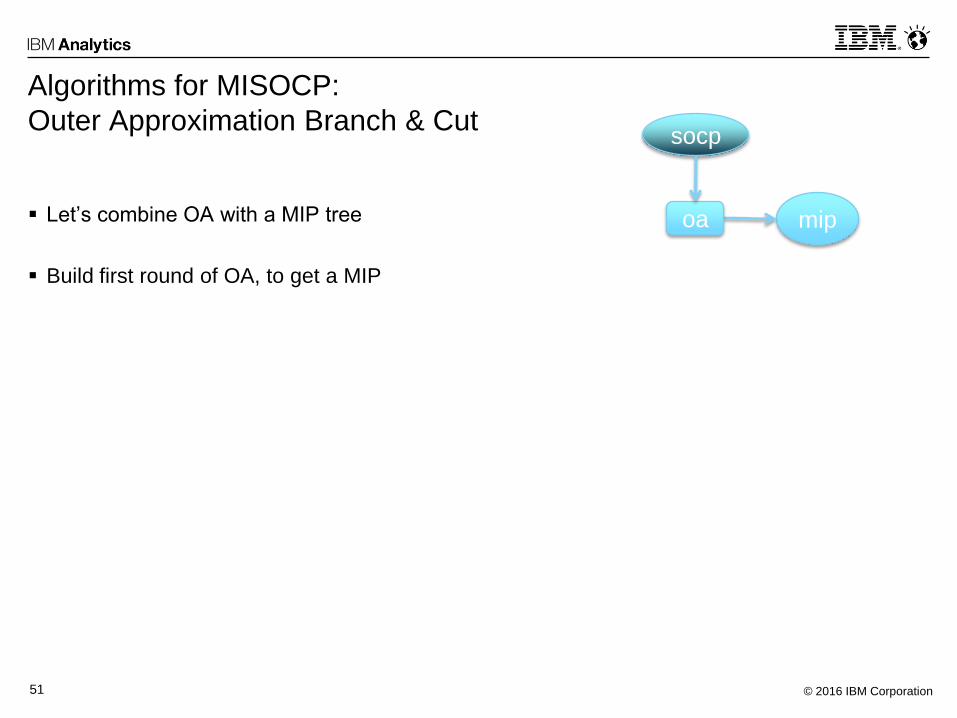
Algorithms for MISOCP:
Outer Approximation Branch & Cut
Let’s combine OA with a MIP tree
Build first round of OA, to get a MIP
mip
socp
oa
© 2016 IBM Corporation52
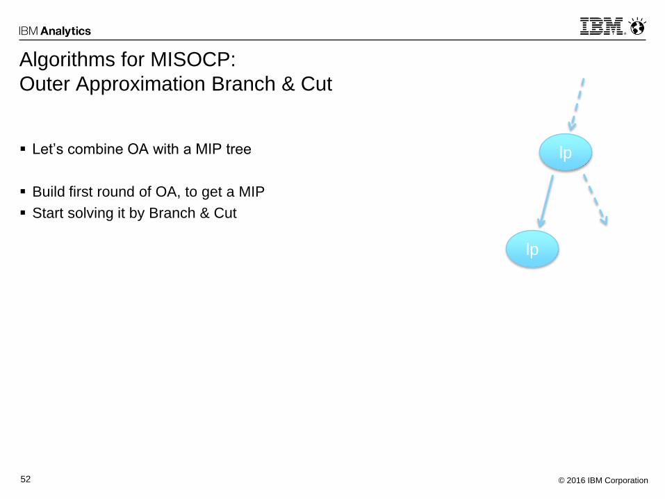
Algorithms for MISOCP:
Outer Approximation Branch & Cut
Let’s combine OA with a MIP tree
Build first round of OA, to get a MIP
Start solving it by Branch & Cut
lp
lp
© 2016 IBM Corporation53
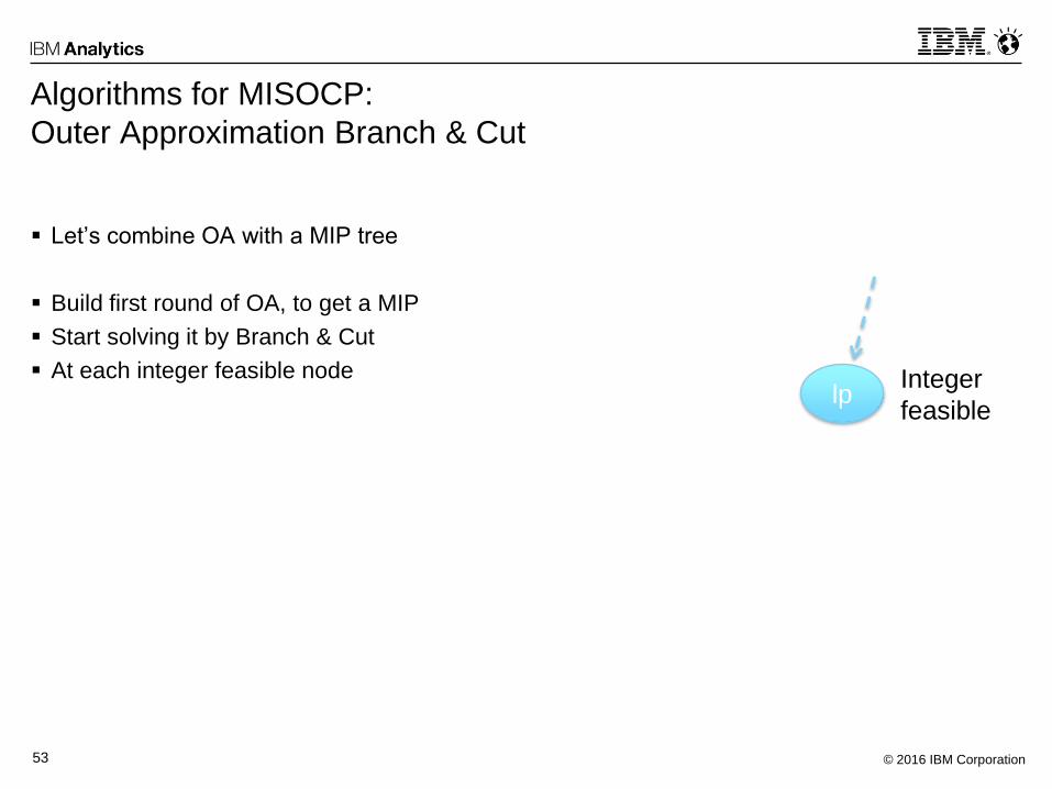
Algorithms for MISOCP:
Outer Approximation Branch & Cut
Let’s combine OA with a MIP tree
Build first round of OA, to get a MIP
Start solving it by Branch & Cut
At each integer feasible nodelp
Integer
feasible
© 2016 IBM Corporation54
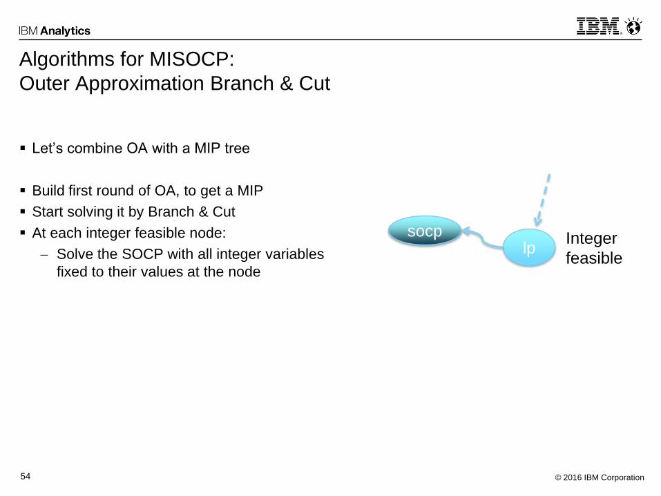
Algorithms for MISOCP:
Outer Approximation Branch & Cut
Let’s combine OA with a MIP tree
Build first round of OA, to get a MIP
Start solving it by Branch & Cut
At each integer feasible node:
Solve the SOCP with all integer variables
fixed to their values at the node
lpsocp Integer
feasible
© 2016 IBM Corporation55
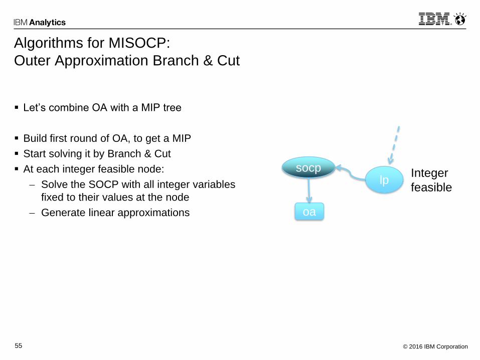
Algorithms for MISOCP:
Outer Approximation Branch & Cut
Let’s combine OA with a MIP tree
Build first round of OA, to get a MIP
Start solving it by Branch & Cut
At each integer feasible node:
Solve the SOCP with all integer variables
fixed to their values at the node
Generate linear approximations
lpsocp
oa
Integer
feasible
© 2016 IBM Corporation56
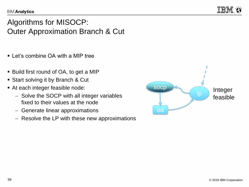
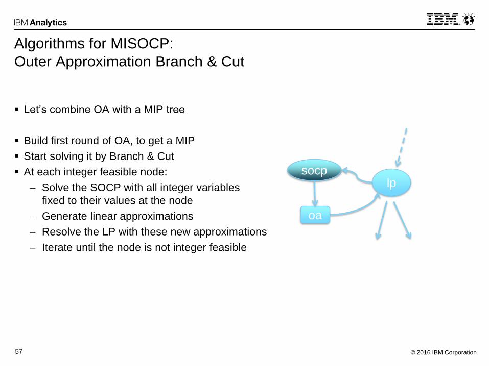
Algorithms for MISOCP:
Outer Approximation Branch & Cut
Let’s combine OA with a MIP tree
Build first round of OA, to get a MIP
Start solving it by Branch & Cut
At each integer feasible node:
Solve the SOCP with all integer variables
fixed to their values at the node
Generate linear approximations
Resolve the LP with these new approximations
lpsocp
oa
Integer
feasible
© 2016 IBM Corporation57
Algorithms for MISOCP:
Outer Approximation Branch & Cut
Let’s combine OA with a MIP tree
Build first round of OA, to get a MIP
Start solving it by Branch & Cut
At each integer feasible node:
Solve the SOCP with all integer variables
fixed to their values at the node
Generate linear approximations
Resolve the LP with these new approximations
Iterate until the node is not integer feasible
lpsocp
oa
© 2016 IBM Corporation58
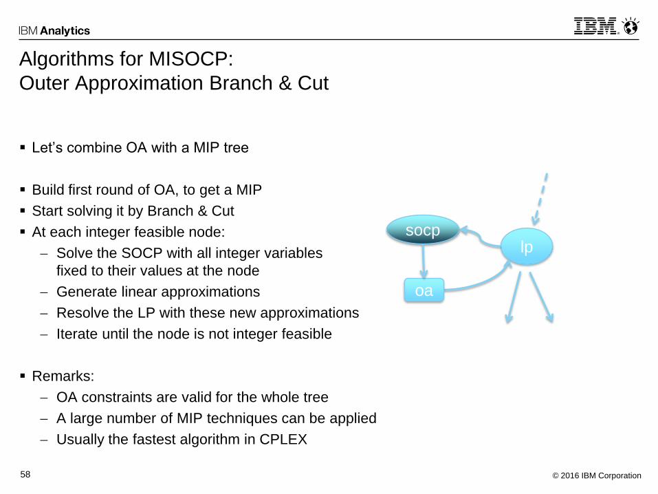
Algorithms for MISOCP:
Outer Approximation Branch & Cut
Let’s combine OA with a MIP tree
Build first round of OA, to get a MIP
Start solving it by Branch & Cut
At each integer feasible node:
Solve the SOCP with all integer variables
fixed to their values at the node
Generate linear approximations
Resolve the LP with these new approximations
Iterate until the node is not integer feasible
Remarks:
OA constraints are valid for the whole tree
A large number of MIP techniques can be applied
Usually the fastest algorithm in CPLEX
lpsocp
oa
© 2016 IBM Corporation59
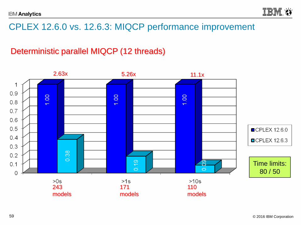
Deterministic parallel MIQCP (12 threads)
243
models
171
models
110
models
Time limits:
80 / 50
2.63x 5.26x 11.1x
CPLEX 12.6.0 vs. 12.6.3: MIQCP performance improvement
© 2016 IBM Corporation60
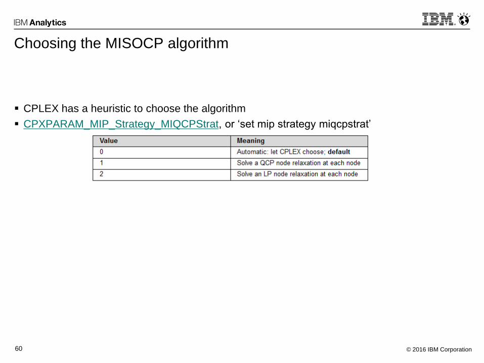
Choosing the MISOCP algorithm
CPLEX has a heuristic to choose the algorithm
CPXPARAM_MIP_Strategy_MIQCPStrat, or ‘set mip strategy miqcpstrat’
© 2016 IBM Corporation61
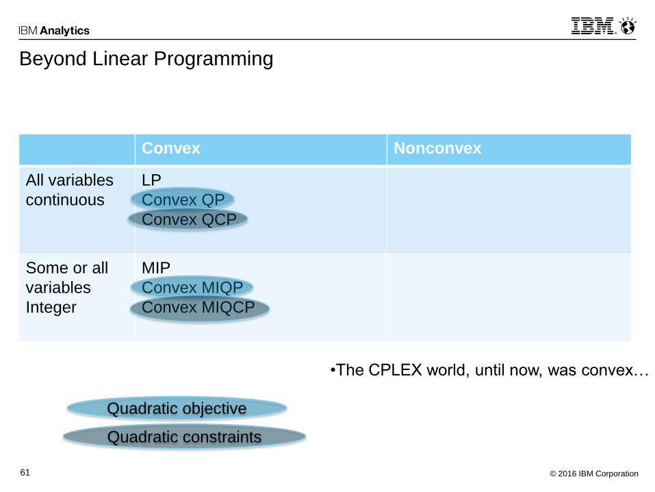
Beyond Linear Programming
Convex Nonconvex
All variables
continuous
LP
Convex QP
Convex QCP
Some or all
variables
Integer
MIP
Convex MIQP
Convex MIQCP
Quadratic objective
Quadratic constraints
•The CPLEX world, until now, was convex…
© 2016 IBM Corporation62
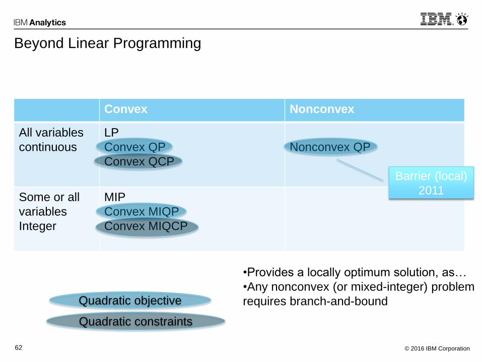
Beyond Linear Programming
Convex Nonconvex
All variables
continuous
LP
Convex QP
Convex QCP
Nonconvex QP
Some or all
variables
Integer
MIP
Convex MIQP
Convex MIQCP
Quadratic objective
Quadratic constraints
Barrier (local)
2011
•Provides a locally optimum solution, as…
•Any nonconvex (or mixed-integer) problem
requires branch-and-bound
© 2016 IBM Corporation63
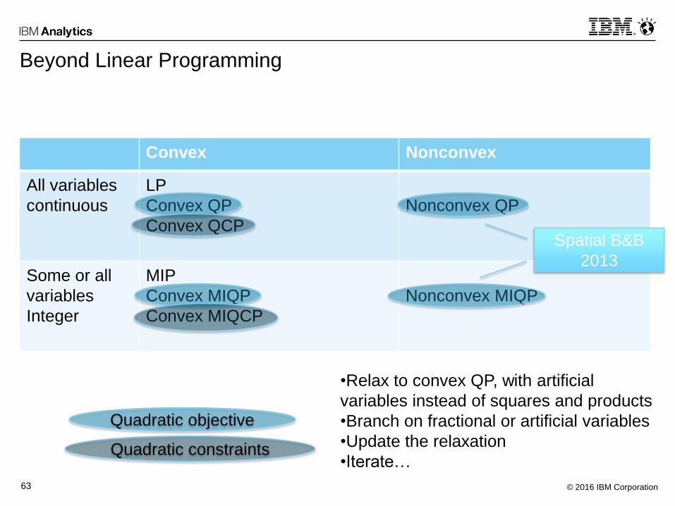
Beyond Linear Programming
Convex Nonconvex
All variables
continuous
LP
Convex QP
Convex QCP
Nonconvex QP
Some or all
variables
Integer
MIP
Convex MIQP
Convex MIQCP
Nonconvex MIQP
Quadratic objective
Quadratic constraints
Spatial B&B
2013
•Relax to convex QP, with artificial
variables instead of squares and products
•Branch on fractional or artificial variables
•Update the relaxation
•Iterate…
© 2016 IBM Corporation64
NONCONVEX (MI)QP
© 2016 IBM Corporation65
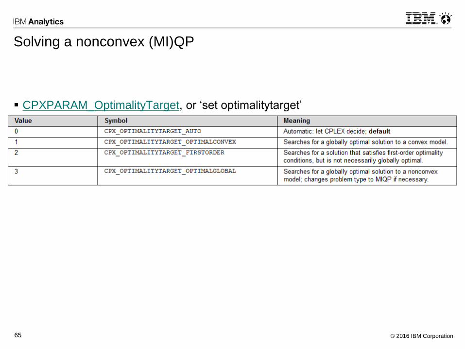
Solving a nonconvex (MI)QP
CPXPARAM_OptimalityTarget, or ‘set optimalitytarget’
© 2016 IBM Corporation66
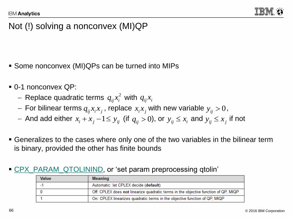
Not (!) solving a nonconvex (MI)QP
Some nonconvex (MI)QPs can be turned into MIPs
0-1 nonconvex QP:
Replace quadratic terms with
For bilinear terms , replace with new variable ,
And add either (if ), or and if not
Generalizes to the cases where only one of the two variables in the bilinear term
is binary, provided the other has finite bounds
CPX_PARAM_QTOLININD, or ‘set param preprocessing qtolin’
2
iij xq
ijji yxx 1
iij xq
jiij xxq ji xx 0ijy
0ijq iij xy jij xy
© 2016 IBM Corporation67
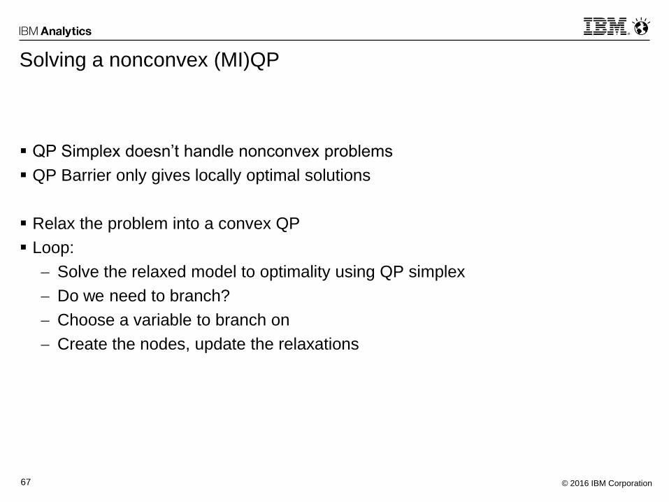
Solving a nonconvex (MI)QP
QP Simplex doesn’t handle nonconvex problems
QP Barrier only gives locally optimal solutions
Relax the problem into a convex QP
Loop:
Solve the relaxed model to optimality using QP simplex
Do we need to branch?
Choose a variable to branch on
Create the nodes, update the relaxations
© 2016 IBM Corporation68
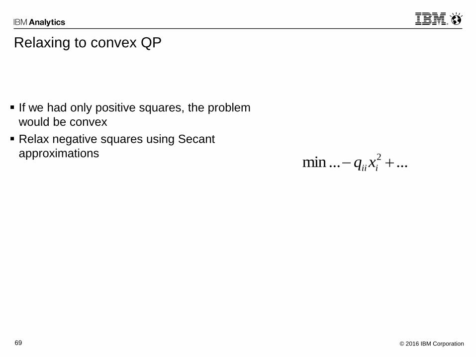
Relaxing to convex QP
If we had only positive squares, the problem
would be convex
© 2016 IBM Corporation69
Relaxing to convex QP
If we had only positive squares, the problem
would be convex
Relax negative squares using Secant
approximations......min 2 iiixq
© 2016 IBM Corporation70
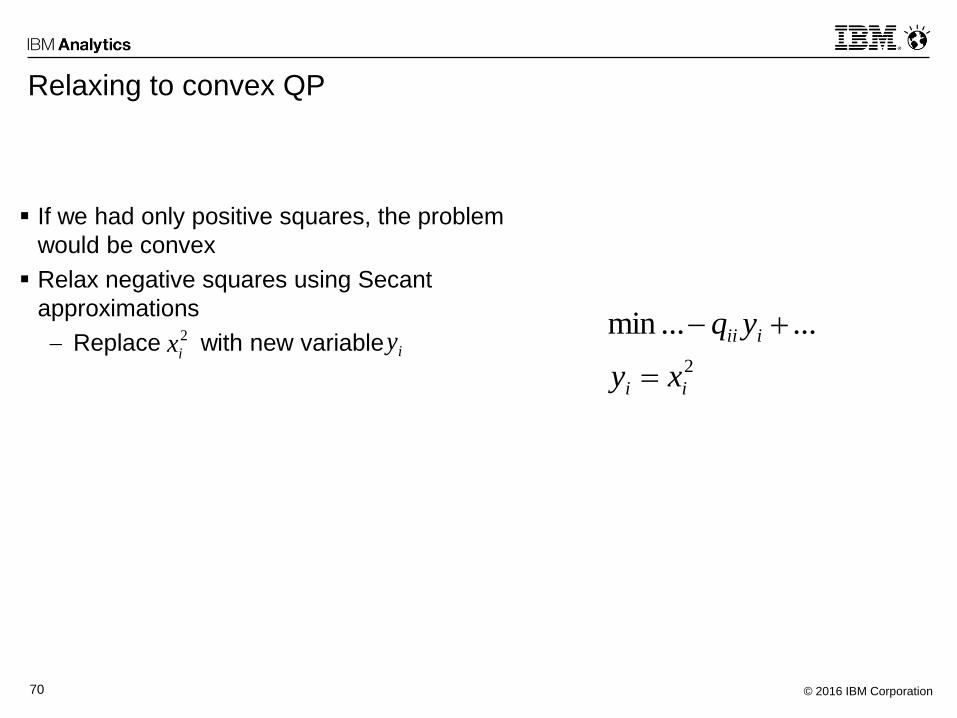
Relaxing to convex QP
If we had only positive squares, the problem
would be convex
Relax negative squares using Secant
approximations
Replace with new variable2
......min
ii
iii
xy
yq
2
ix iy
© 2016 IBM Corporation71
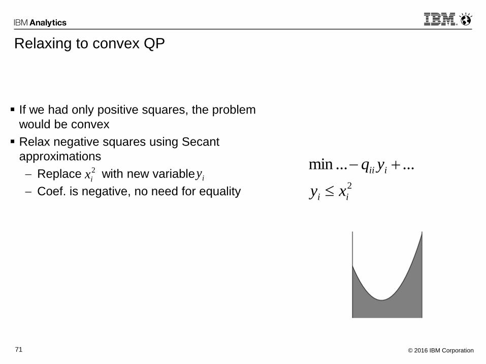
Relaxing to convex QP
If we had only positive squares, the problem
would be convex
Relax negative squares using Secant
approximations
Replace with new variable
Coef. is negative, no need for equality2
......min
ii
iii
xy
yq
2
ix iy
© 2016 IBM Corporation72
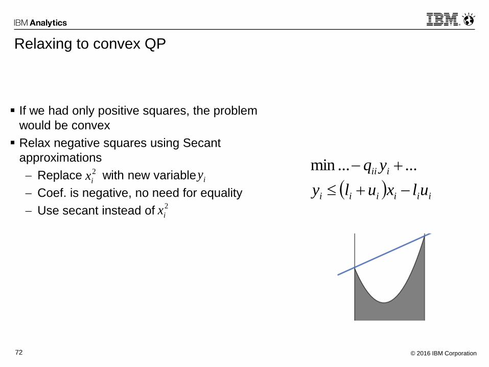
Relaxing to convex QP
iiiiii
iii
ulxuly
yq
......min
If we had only positive squares, the problem
would be convex
Relax negative squares using Secant
approximations
Replace with new variable
Coef. is negative, no need for equality
Use secant instead of
2
ix iy
2
ix
© 2016 IBM Corporation73
Relaxing to convex QP
iiiiii
iii
ulxuly
yq
......min
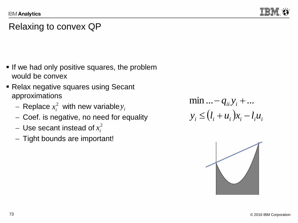
If we had only positive squares, the problem
would be convex
Relax negative squares using Secant
approximations
Replace with new variable
Coef. is negative, no need for equality
Use secant instead of
Tight bounds are important!
2
ix iy
2
ix
© 2016 IBM Corporation74
Relaxing to convex QP
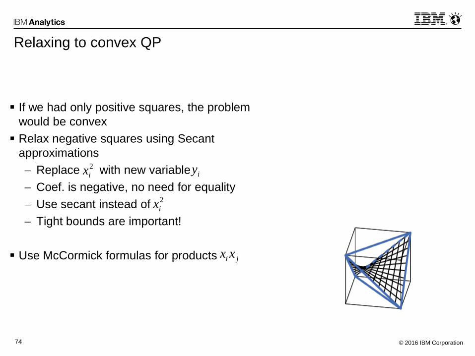
If we had only positive squares, the problem
would be convex
Relax negative squares using Secant
approximations
Replace with new variable
Coef. is negative, no need for equality
Use secant instead of
Tight bounds are important!
Use McCormick formulas for products
2
ix iy
2
ix
ji xx
© 2016 IBM Corporation75
Relaxing to convex QP
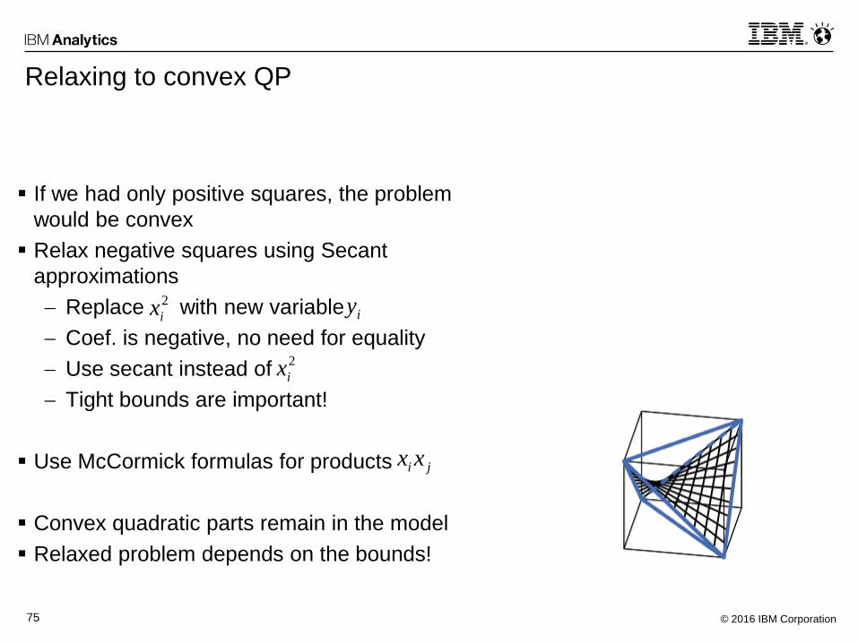
If we had only positive squares, the problem
would be convex
Relax negative squares using Secant
approximations
Replace with new variable
Coef. is negative, no need for equality
Use secant instead of
Tight bounds are important!
Use McCormick formulas for products
Convex quadratic parts remain in the model
Relaxed problem depends on the bounds!
2
ix iy
2
ix
ji xx
© 2016 IBM Corporation76
Branching
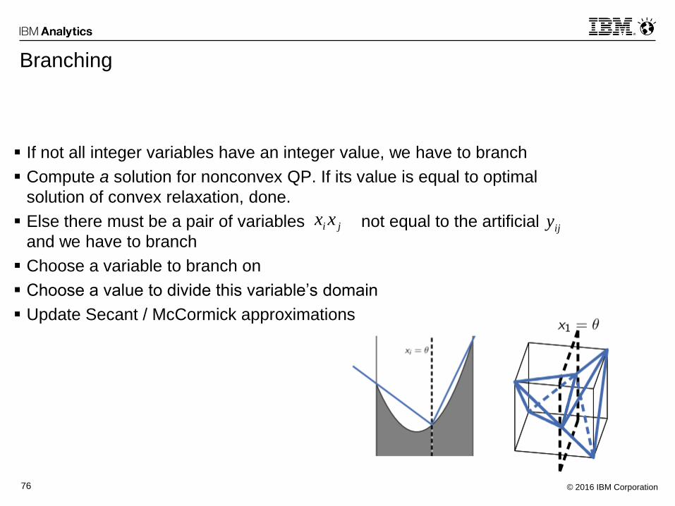
If not all integer variables have an integer value, we have to branch
Compute a solution for nonconvex QP. If its value is equal to optimal
solution of convex relaxation, done.
Else there must be a pair of variables not equal to the artificial
and we have to branch
Choose a variable to branch on
Choose a value to divide this variable’s domain
Update Secant / McCormick approximations
ji xxijy
© 2016 IBM Corporation77
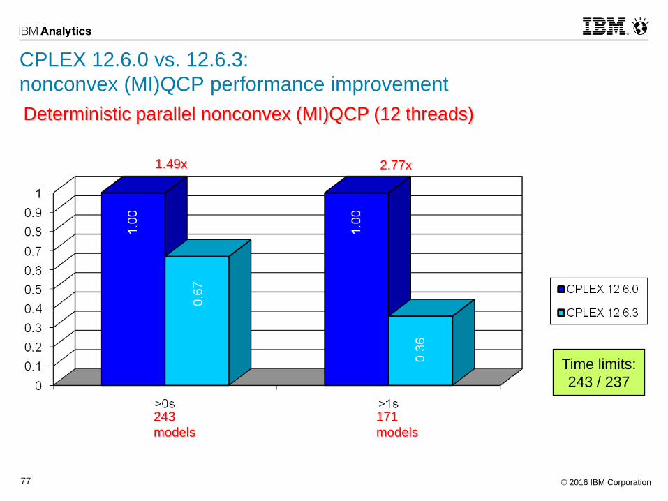
Deterministic parallel nonconvex (MI)QCP (12 threads)
243
models
171
models
Time limits:
243 / 237
1.49x 2.77x
CPLEX 12.6.0 vs. 12.6.3:
nonconvex (MI)QCP performance improvement
© 2016 IBM Corporation78
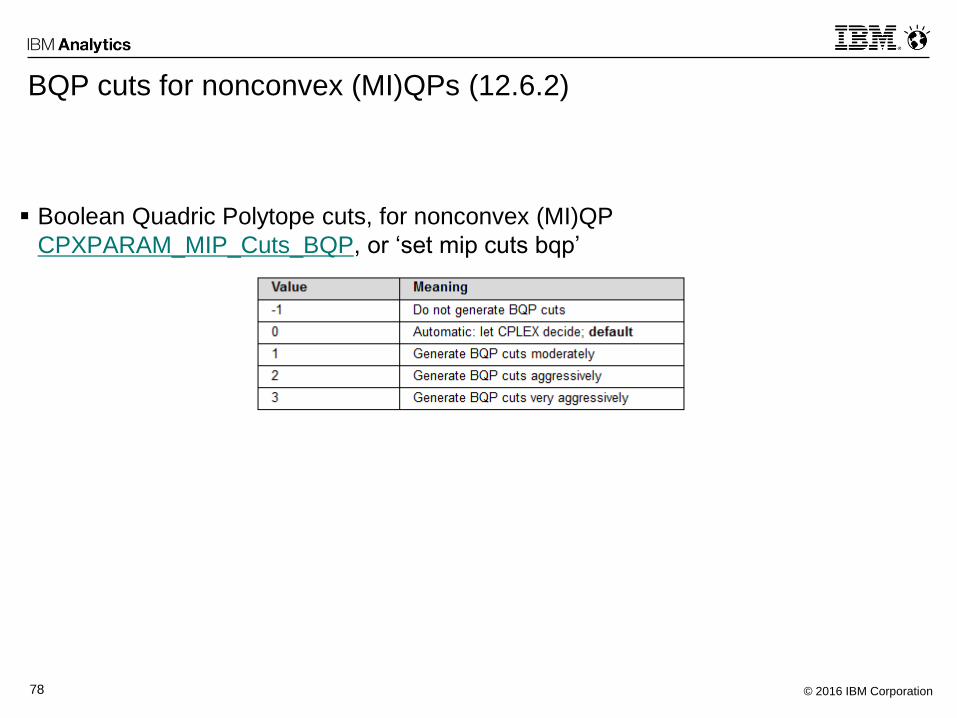
BQP cuts for nonconvex (MI)QPs (12.6.2)
Boolean Quadric Polytope cuts, for nonconvex (MI)QP
CPXPARAM_MIP_Cuts_BQP, or ‘set mip cuts bqp’
© 2016 IBM Corporation79
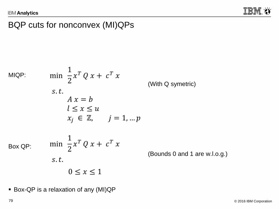
BQP cuts for nonconvex (MI)QPs
MIQP:
(With Q symetric)
Box QP:
(Bounds 0 and 1 are w.l.o.g.)
Box-QP is a relaxation of any (MI)QP
© 2016 IBM Corporation80
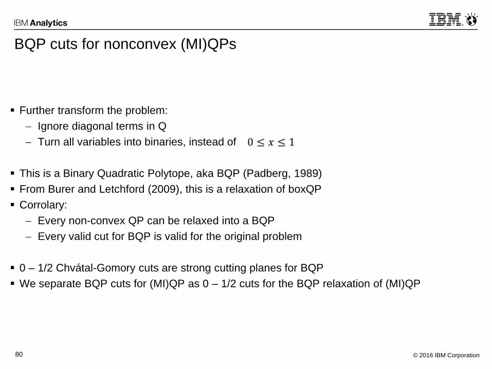
BQP cuts for nonconvex (MI)QPs
Further transform the problem:
Ignore diagonal terms in Q
Turn all variables into binaries, instead of
This is a Binary Quadratic Polytope, aka BQP (Padberg, 1989)
From Burer and Letchford (2009), this is a relaxation of boxQP
Corrolary:
Every non-convex QP can be relaxed into a BQP
Every valid cut for BQP is valid for the original problem
0 – 1/2 Chvátal-Gomory cuts are strong cutting planes for BQP
We separate BQP cuts for (MI)QP as 0 – 1/2 cuts for the BQP relaxation of (MI)QP
© 2016 IBM Corporation81
MISC. FEATURES
© 2016 IBM Corporation82
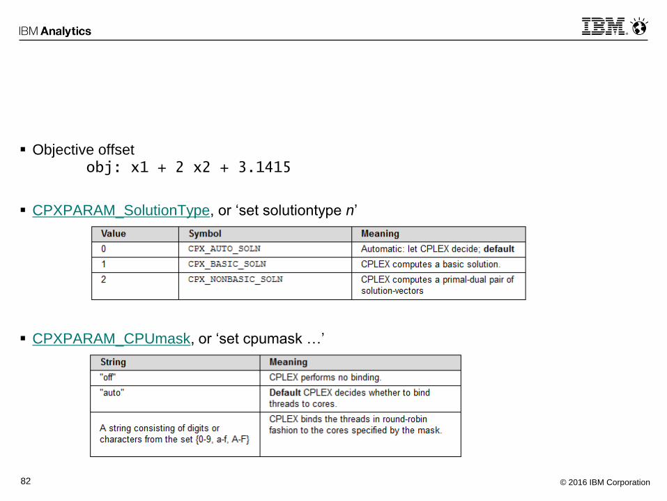
Objective offset
obj: x1 + 2 x2 + 3.1415
CPXPARAM_SolutionType, or ‘set solutiontype n’
CPXPARAM_CPUmask, or ‘set cpumask …’
© 2016 IBM Corporation83
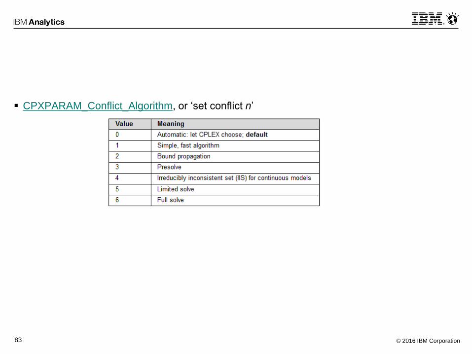
CPXPARAM_Conflict_Algorithm, or ‘set conflict n’
© 2016 IBM Corporation84
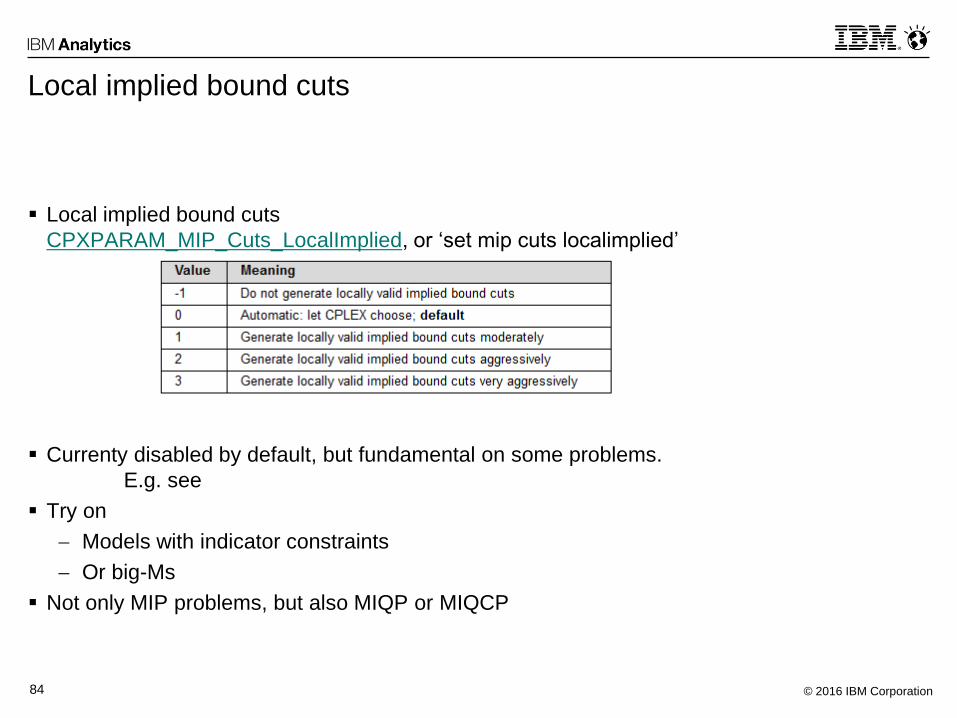
Local implied bound cuts
Local implied bound cuts
CPXPARAM_MIP_Cuts_LocalImplied, or ‘set mip cuts localimplied’
Currenty disabled by default, but fundamental on some problems.
E.g. see
Try on
Models with indicator constraints
Or big-Ms
Not only MIP problems, but also MIQP or MIQCP
© 2016 IBM Corporation85
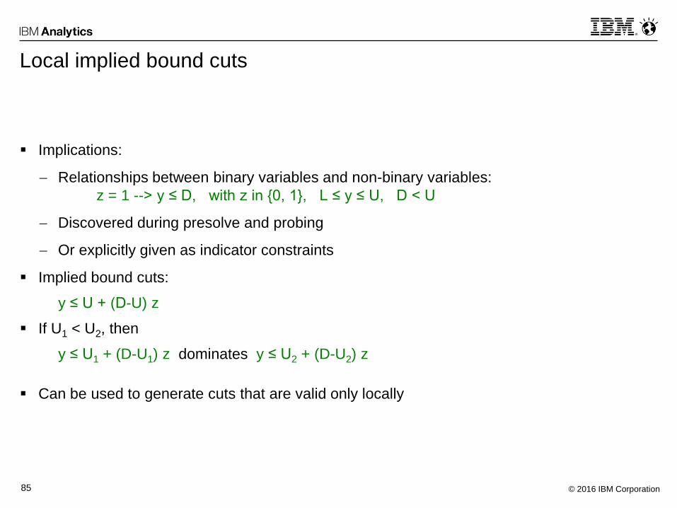
Local implied bound cuts
Implications:
Relationships between binary variables and non-binary variables:
z = 1 --> y ≤ D, with z in {0, 1}, L ≤ y ≤ U, D < U
Discovered during presolve and probing
Or explicitly given as indicator constraints
Implied bound cuts:
y ≤ U + (D-U) z
If U1 < U2, then
y ≤ U1 + (D-U1) z dominates y ≤ U2 + (D-U2) z
Can be used to generate cuts that are valid only locally
© 2016 IBM Corporation86
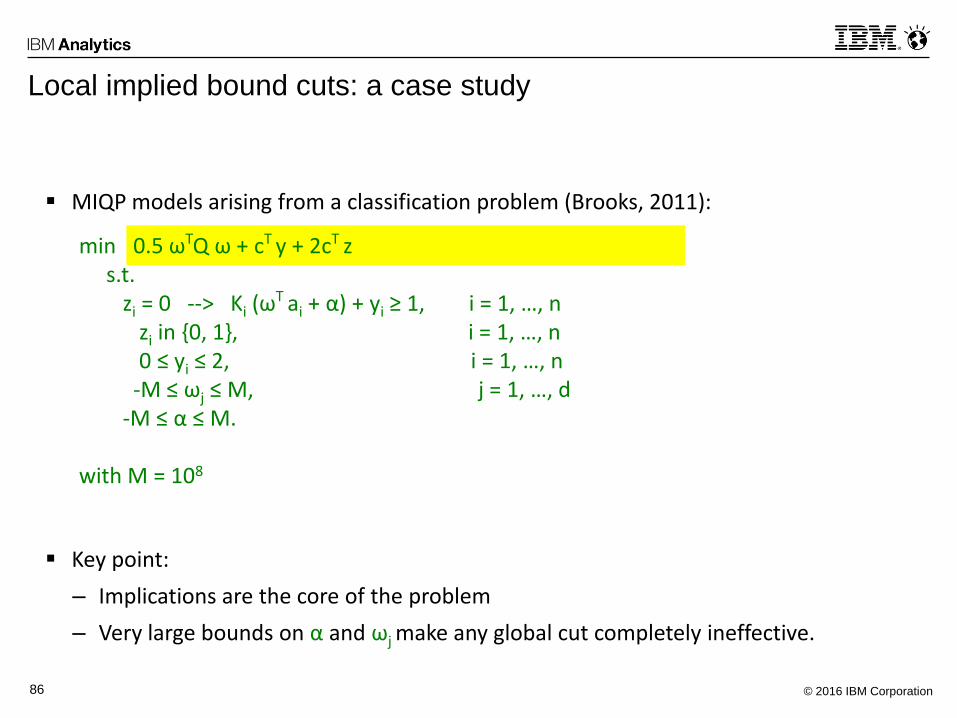
MIQP models arising from a classification problem (Brooks, 2011):
Key point:
– Implications are the core of the problem
– Very large bounds on α and ωj make any global cut completely ineffective.
min 0.5 ωTQ ω + cT y + 2cT z s.t.
zi = 0 --> Ki (ωT ai + α) + yi ≥ 1, i = 1, …, nzi in {0, 1}, i = 1, …, n0 ≤ yi ≤ 2, i = 1, …, n
-M ≤ ωj ≤ M, j = 1, …, d-M ≤ α ≤ M.
with M = 108
Local implied bound cuts: a case study
© 2016 IBM Corporation87
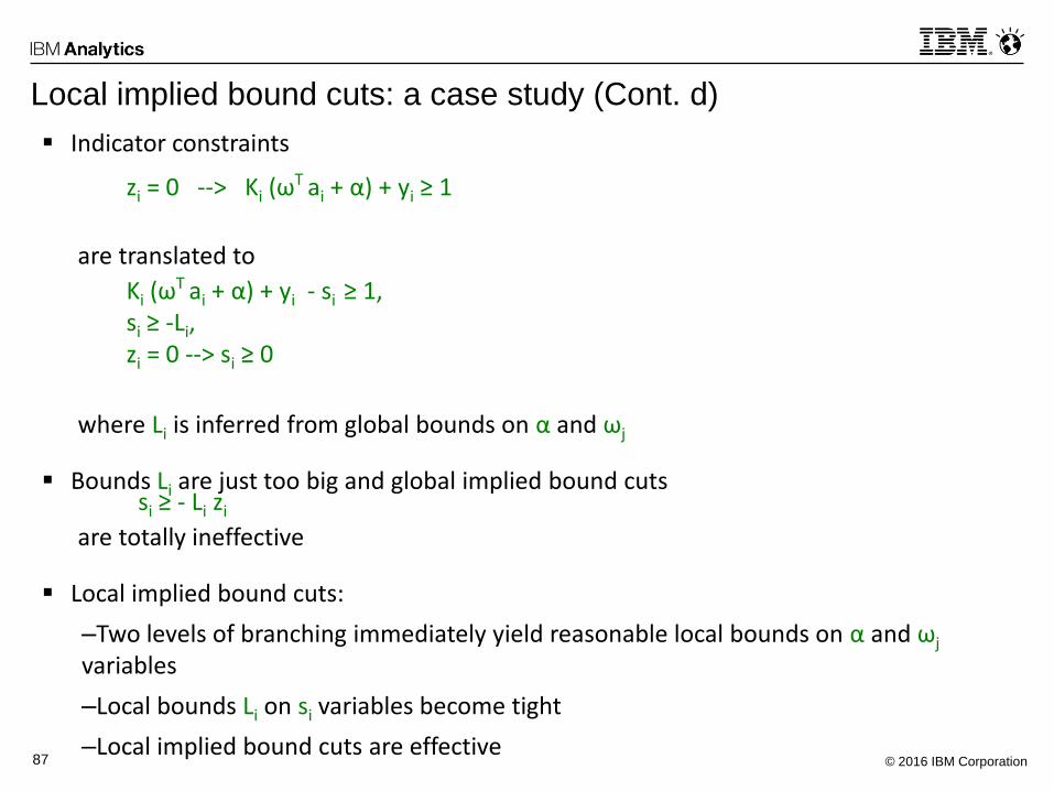
Indicator constraints
are translated to
where Li is inferred from global bounds on α and ωj
Bounds Li are just too big and global implied bound cuts
are totally ineffective
Local implied bound cuts:
–Two levels of branching immediately yield reasonable local bounds on α and ωj
variables
–Local bounds Li on si variables become tight
–Local implied bound cuts are effective
Local implied bound cuts: a case study (Cont. d)
zi = 0 --> Ki (ωT ai + α) + yi ≥ 1
Ki (ωT ai + α) + yi - si ≥ 1,si ≥ -Li, zi = 0 --> si ≥ 0
si ≥ - Li zi
© 2016 IBM Corporation88
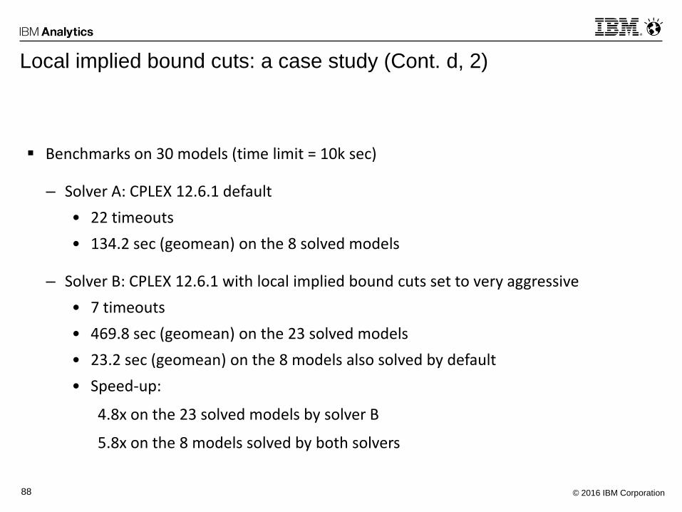
Benchmarks on 30 models (time limit = 10k sec)
– Solver A: CPLEX 12.6.1 default
• 22 timeouts
• 134.2 sec (geomean) on the 8 solved models
– Solver B: CPLEX 12.6.1 with local implied bound cuts set to very aggressive
• 7 timeouts
• 469.8 sec (geomean) on the 23 solved models
• 23.2 sec (geomean) on the 8 models also solved by default
• Speed-up:
4.8x on the 23 solved models by solver B
5.8x on the 8 models solved by both solvers
Local implied bound cuts: a case study (Cont. d, 2)

© 2016 IBM Corporation89
UNDER THE HOOD…
© 2016 IBM Corporation90
Constraint disaggregation (12.6.1)
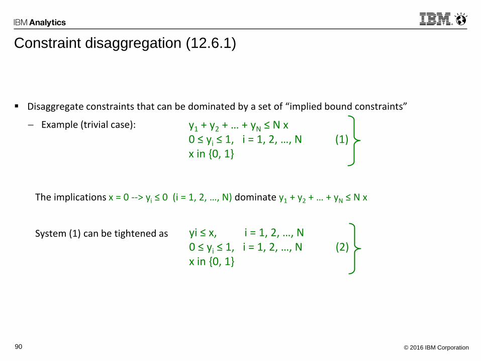
Disaggregate constraints that can be dominated by a set of “implied bound constraints”
Example (trivial case):
The implications x = 0 --> yi ≤ 0 (i = 1, 2, …, N) dominate y1 + y2 + … + yN ≤ N x
System (1) can be tightened as
y1 + y2 + … + yN ≤ N x0 ≤ yi ≤ 1, i = 1, 2, …, N (1)x in {0, 1}
yi ≤ x, i = 1, 2, …, N0 ≤ yi ≤ 1, i = 1, 2, …, N (2)x in {0, 1}
© 2016 IBM Corporation91
Constraint disaggregation
Trade off between tightening and number of non zeros added
The larger is N, the larger is the expected tightening
Disaggregating a constraint of length N implies adding N-1 rows and N-1 non zeros
Applied rather conservatively
Only 16% of hard models (≥ 100 sec) affected
10-14% speed-up on the affected models
9
1
© 2016 IBM Corporation92
Propagation of Quadratic constraints and objective (12.6.1)
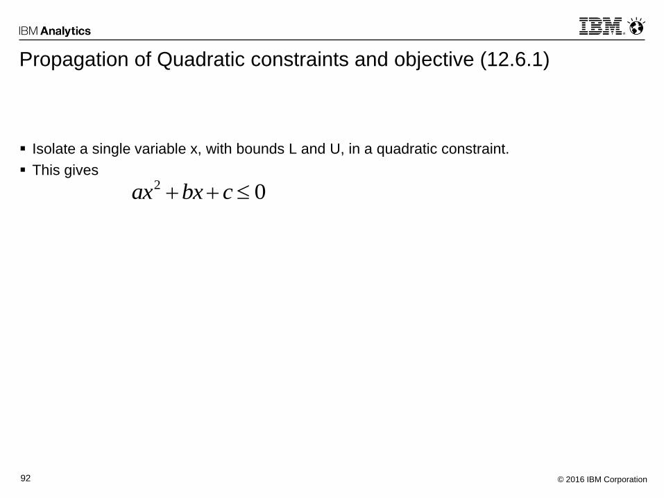
Isolate a single variable x, with bounds L and U, in a quadratic constraint.
This gives
02 cbxax
© 2016 IBM Corporation93
Propagation of Quadratic constraints and objective
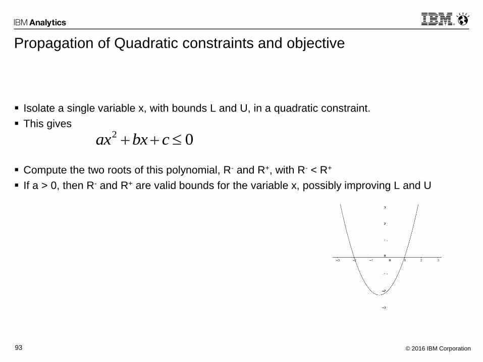
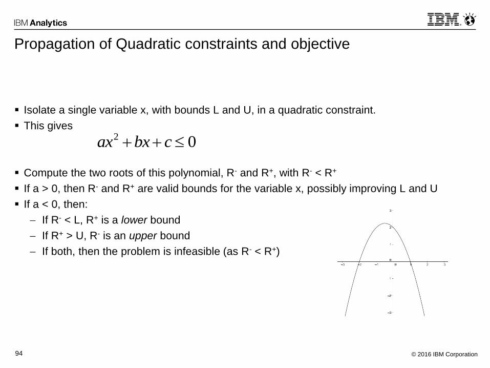
Isolate a single variable x, with bounds L and U, in a quadratic constraint.
This gives
Compute the two roots of this polynomial, R- and R+, with R- < R+
If a > 0, then R- and R+ are valid bounds for the variable x, possibly improving L and U
02 cbxax
© 2016 IBM Corporation94
Propagation of Quadratic constraints and objective
Isolate a single variable x, with bounds L and U, in a quadratic constraint.
This gives
Compute the two roots of this polynomial, R- and R+, with R- < R+
If a > 0, then R- and R+ are valid bounds for the variable x, possibly improving L and U
If a < 0, then:
If R- < L, R+ is a lower bound
If R+ > U, R- is an upper bound
If both, then the problem is infeasible (as R- < R+)
02 cbxax
© 2016 IBM Corporation95
Propagation of Quadratic constraints and objective
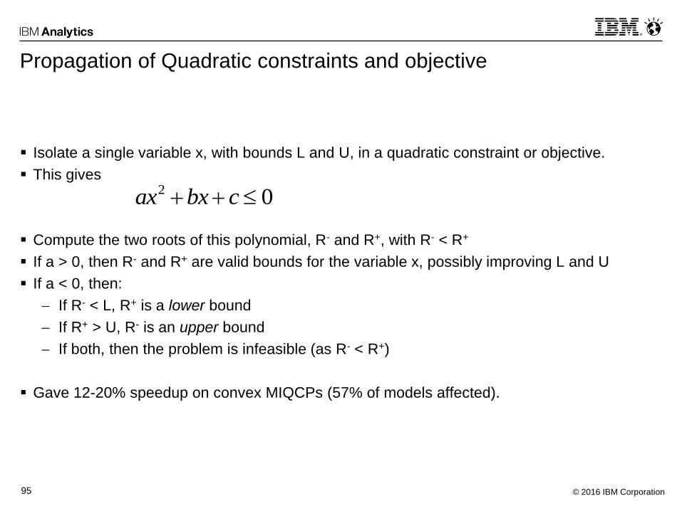
Isolate a single variable x, with bounds L and U, in a quadratic constraint or objective.
This gives
Compute the two roots of this polynomial, R- and R+, with R- < R+
If a > 0, then R- and R+ are valid bounds for the variable x, possibly improving L and U
If a < 0, then:
If R- < L, R+ is a lower bound
If R+ > U, R- is an upper bound
If both, then the problem is infeasible (as R- < R+)
Gave 12-20% speedup on convex MIQCPs (57% of models affected).
02 cbxax
© 2016 IBM Corporation96
Cone disaggregation (12.6.2)
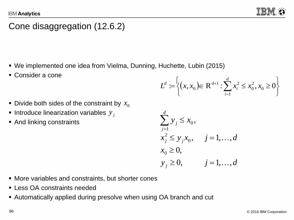
We implemented one idea from Vielma, Dunning, Huchette, Lubin (2015)
Consider a cone
Divide both sides of the constraint by
Introduce linearization variables
And linking constraints
More variables and constraints, but shorter cones
Less OA constraints needed
Automatically applied during presolve when using OA branch and cut
0,:R,: 0
2
0
1
21d
0 xxxxxLd
i
i
d
djy
x
djxyx
xy
j
jj
d
j
j
,,1,0
,0
,,1,
,
0
0
2
0
1
0x
jy
© 2016 IBM Corporation97
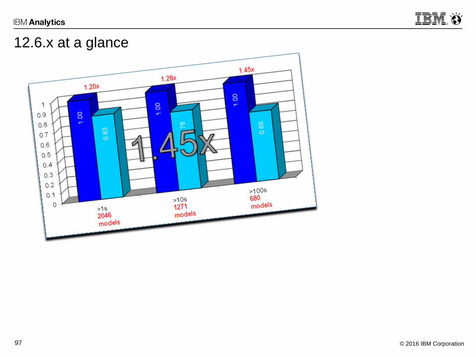
12.6.x at a glance
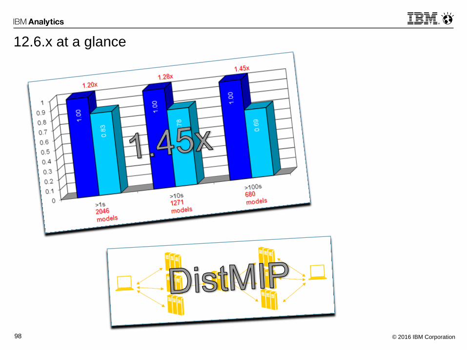
© 2016 IBM Corporation98
12.6.x at a glance
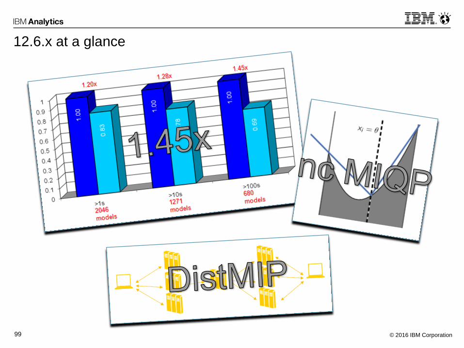
© 2016 IBM Corporation99
12.6.x at a glance
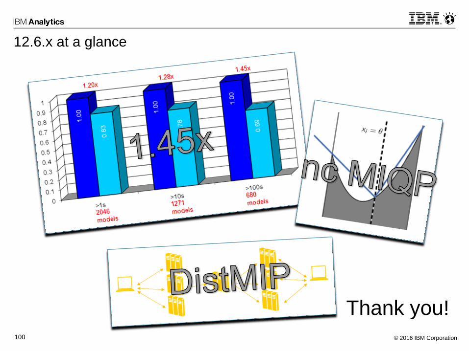
© 2016 IBM Corporation100
12.6.x at a glance
Thank you!

© 2016 IBM Corporation102
Legal Disclaimer
• © IBM Corporation 2015. All Rights Reserved.
• The information contained in this publication is provided for informational purposes only. While efforts were made to verify
the completeness and accuracy of the information contained in this publication, it is provided AS IS without warranty of any
kind, express or implied. In addition, this information is based on IBM’s current product plans and strategy, which are
subject to change by IBM without notice. IBM shall not be responsible for any damages arising out of the use of, or
otherwise related to, this publication or any other materials. Nothing contained in this publication is intended to, nor shall
have the effect of, creating any warranties or representations from IBM or its suppliers or licensors, or altering the terms
and conditions of the applicable license agreement governing the use of IBM software.
• References in this presentation to IBM products, programs, or services do not imply that they will be available in all
countries in which IBM operates. Product release dates and/or capabilities referenced in this presentation may change at
any time at IBM’s sole discretion based on market opportunities or other factors, and are not intended to be a commitment
to future product or feature availability in any way. Nothing contained in these materials is intended to, nor shall have the
effect of, stating or implying that any activities undertaken by you will result in any specific sales, revenue growth or other
results.
• Performance is based on measurements and projections using standard IBM benchmarks in a controlled environment.
The actual throughput or performance that any user will experience will vary depending upon many factors, including
considerations such as the amount of multiprogramming in the user's job stream, the I/O configuration, the storage
configuration, and the workload processed. Therefore, no assurance can be given that an individual user will achieve
results similar to those stated here.
• IBM, the IBM logo, CPLEX Optimizer, CPLEX Optimization Studio are trademarks of International Business Machines
Corporation in the United States, other countries, or both. Unyte is a trademark of WebDialogs, Inc., in the United States,
other countries, or both.
• If you reference Intel® and/or any of the following Intel products in the text, please mark the first use and include those that
you use as follows; otherwise delete:
Intel, Intel Centrino, Celeron, Intel Xeon, Intel SpeedStep, Itanium, and Pentium are trademarks or registered trademarks
of Intel Corporation or its subsidiaries in the United States and other countries.