the craft of fractional modelling in science and engineering
TRANSCRIPT

The Craft of Fractional Modelling in Science and Engineering
Jordan Hristov
www.mdpi.com/journal/fractalfract
Edited by
Printed Edition of the Special Issue Published in Fractal Fract
fractal and fractional

The Craft of Fractional Modelling in
Science and Engineering
Special Issue EditorJordan Hristov
MDPI • Basel • Beijing • Wuhan • Barcelona • Belgrade

Special Issue Editor
Jordan Hristov
University of Chemical Technology and Metallurgy
Bulgaria
Editorial Office
MDPI
St. Alban-Anlage 66
Basel, Switzerland
This edition is a reprint of the Special Issue published online in the open access journal Fractal
Fract (ISSN 2504-3110) from 2017–2018 (available at: http://www.mdpi.com/journal/fractalfract/
special issues/Fractional Modelling).
For citation purposes, cite each article independently as indicated on the article page online and as
indicated below:
Lastname, F.M.; Lastname, F.M. Article title. Journal Name Year, Article number, page range.
First Edition 2018
ISBN 978-3-03842-983-8 (Pbk)
ISBN 978-3-03842-984-5 (PDF)
Articles in this volume are Open Access and distributed under the Creative Commons Attribution
(CC BY) license, which allows users to download, copy and build upon published articles even
for commercial purposes, as long as the author and publisher are properly credited, which ensures
maximum dissemination and a wider impact of our publications. The book taken as a whole is c© 2018
MDPI, Basel, Switzerland, distributed under the terms and conditions of the Creative Commons
license CC BY-NC-ND (http://creativecommons.org/licenses/by-nc-nd/4.0/).

Table of Contents
About the Special Issue Editor . . . . . . . . . . . . . . . . . . . . . . . . . . . . . . . . . . . . . . v
Dimiter Prodanov
Fractional Velocity as a Tool for the Study of Non-Linear Problemsdoi:10.3390/fractalfract2010004 . . . . . . . . . . . . . . . . . . . . . . . . . . . . . . . . . . . . 1
Sachin Bhalekar and Jayvant Patadee
Series Solution of the Pantograph Equation and Its Propertiesdoi:10.3390/fractalfract1010016 . . . . . . . . . . . . . . . . . . . . . . . . . . . . . . . . . . . . 24
Mehmet Yavuz and Necati Ozdemir
European Vanilla Option Pricing Model of Fractional Order without Singular Kerneldoi:10.3390/fractalfract2010003 . . . . . . . . . . . . . . . . . . . . . . . . . . . . . . . . . . . . 36
Jose Francisco Gomez-Aguilar, Abdon Atangana
Fractional Derivatives with the Power-Law and the Mittag–Leffler Kernel Applied to theNonlinear Baggs–Freedman Modeldoi:10.3390/fractalfract2010010 . . . . . . . . . . . . . . . . . . . . . . . . . . . . . . . . . . . . 47
Xavier Moreau, Roy Abi Zeid Daou and Fady Christophy
Comparison between the Second and Third Generations of the CRONE Controller:Application to a Thermal Diffusive Interface Mediumdoi:10.3390/fractalfract2010005 . . . . . . . . . . . . . . . . . . . . . . . . . . . . . . . . . . . . 61
D. Vivek, K. Kanagarajan and Seenith Sivasundaram
Dynamics and Stability Results for Hilfer Fractional Type Thermistor Problemdoi:10.3390/fractalfract1010005 . . . . . . . . . . . . . . . . . . . . . . . . . . . . . . . . . . . . 80
Rafał Brociek, Damian Słota, Mariusz Krol, Grzegorz Matula and Waldemar Kwasny
Modeling of Heat Distribution in Porous Aluminum Using Fractional Differential Equationdoi:10.3390/fractalfract1010017 . . . . . . . . . . . . . . . . . . . . . . . . . . . . . . . . . . . . 94
Ervin K. Lenzi, Andrea Ryba and Marcelo K. Lenzi
Monitoring Liquid-Liquid Mixtures Using Fractional Calculus and Image Analysisdoi:10.3390/fractalfract2010011 . . . . . . . . . . . . . . . . . . . . . . . . . . . . . . . . . . . . 103
Emilia Bazhlekova and Ivan Bazhlekov
Stokes’ First Problem for Viscoelastic Fluids with a Fractional Maxwell Modeldoi:10.3390/fractalfract1010007 . . . . . . . . . . . . . . . . . . . . . . . . . . . . . . . . . . . . 115
iii
Preface to ”The Craft of Fractional Modelling in Science and Engineering” . . . . . . . . . . . vii


About the Special Issue Editor
Jordan Hristov is a professor of Chemical Engineering with the University of Chemical Technology
and Metallurgy, Sofia, Bulgaria. He graduated from the Technical University, Sofia, as an electrical
engineer and was awarded his Ph.D. degree in chemical engineering in 1994 with a thesis in the field
of magnetic field assisted fluidization. His Doctor of Sciences thesis on nonlinear and anomalous
diffusion models was successfully completed in 2018. Prof. Hristov has more than 39 years’ experience
in the field of chemical engineering with principle research interests in mechanics of particulate
materials, fluidization, magnetic field effects of process intensification, mathematical modelling in
complex systems, non-linear diffusion and fractional calculus application in modelling with more than
170 articles published in international journals. He is an editorial board member of Thermal Science,
Particuology, Progress in Fractional Differentiation and Applications and Fractional and Fractal.
v


Preface to ”The Craft of Fractional Modelling in
Science and Engineering”
vii
Fractional calculus has performed an important role in the fields of mathematics, physics,electronics, mechanics, and engineering in recent years. The modeling methods involving fractionaloperators have been continuously generalized and enhanced, especially during the last few decades.Many operations in physics and engineering can be defined accurately by using systems of differentialequations containing different types of fractional derivatives.
This book is a result of the contributions of scientists involved in the special collection of articlesorganized by the journal Fractal and Fractional (MDPI), most of which have been published at the endof 2017 and the beginning 2018. In accordance with the initial idea of a Special Issue, the best publishedhave now been consolidated into this book.
The articles included span a broad area of applications of fractional calculus and demonstrate thefeasibility of the non-integer differentiation and integration approach in modeling directly related topertinent problems in science and engineering. It is worth mentioning some principle results fromthe collected articles, now presented as book chapters, which make this book a contemporary andinteresting read for a wide audience:
The fractional velocity concept developed by Prodanov [1] is demonstrated as tool to characterizeHölder and in particular, singular functions. Fractional velocities are defined as limits of the differencequotients of a fractional power and they generalize the local notion of a derivative. On the otherhand, their properties contrast some of the usual properties of derivatives. One of the most peculiarproperties of these operators is that the set of their nontrivial values is disconnected. This can be used,for example, to model instantaneous interactions, such as Langevin dynamics. In this context, the localfractional derivatives and the equivalent fractional velocities have several distinct properties comparedto integer-order derivatives.
The classical pantograph equation and its generalizations, including fractional order and higherorder cases, is developed by Bhalekar and Patade [2]. The special functions are obtained from the seriessolution of these equations. Different properties of these special functions are established, andtheirrelations with other functions are developed.
The new direction in fractional calculus involving nonsingular memory kernels, developed in thelast three years following the seminar articles of Caputo and Fabrizio in 2015 [3], is hot research topic.Two studies in the collection clearly demonstrate two principle directions: operators with nonsingularexponential kernels, i.e., the so-called Caputo-Fabrizio derivatives [4,5] (Hristov, 2016, Chapter 10),and operators with nonsingular memory kernels based on the Mittag-Leffler function [6,7] (Atangana,Baleanu, 2016; Baleanu, Fennandez, 2018).
Yavuz and Ozdemir [8] demonstrate a novel approximate-analytical solution method, called theLaplace homotopy analysis method (LHAM), using the Caputo-Fabrizio (CF) fractional derivativeoperator based on the exponential kernel. The recommended method is obtained by combining Laplacetransform (LT) and the homotopy analysis method (HAM). This study considers the application ofLHAM to obtain solutions of the fractional Black-Scholes equations (FBSEs) with the Caputo-Fabrizio(CF) fractional derivative and appropriate initial conditions. The authors demonstrate the efficienciesand accuracies of the suggested method by applying it to the FBS option pricing models with theirinitial conditions satisfied by the classical European vanilla option. Using real market values fromfinance literature, it is demonstrated how the option is priced for fractional cases of European call optionpricing models. Moreover, the proposed fractional model allows modeling of the price of differentfinancial derivatives such as swaps, warrant, etc., in complete agreement with the correspondingexact solutions.

viii
In light of new fractional operators, Gomez-Aguilar and Atangana [9] present alternativerepresentations of the Freedman model considering Liouville-Caputo and Atangana-Baleanu-Caputofractional derivatives. The solutions of these alternative models are obtained using an iterative schemebased on the Laplace transform and the Sumudu transform. Moreover, special solutions via theAdams-Moulton rule are obtained for both fractional derivatives.
In light of certain applied problems, the thermal control of complex thermal interfaces and heatconduction are principle issues to which classical fractional calculus is widely applicable. The control ofthermal interfaces has gained importance in recent years because of the high cost of heating and coolingmaterials in many applications. The main focus in the work of Moreau et al. [10] is to compare thesecond and third generations of the CRONE controller (French acronym of Commande Robusted’OrdreNon Entier) in the control of a non-integer plant by means a fractional order controller. The idea isthat, as a consequence of the fractional approach, all of the systems of integer order are replaced bythe implementation of a CRONE controller. The results reveal that the second generation CRONEcontroller is robust when the variations in the plant are modeled with gain changes, whereas the phaseremains the same for all of the plants (even if not constant). However, the third generation CRONEcontroller demonstrates a good, feasible robustness when the parameters of the plant are changed aswell as when both gain and phase variations are encountered.
Thermistors are part of a larger group of passive components. They are temperature-dependentresistors and come in two varieties, negative temperature coefficients (NTCs) and positive temperaturecoefficients (PTCs), although NTCs are most commonly u sed. NTC thermistors are nonlinear, and theirresistance decreases as the temperature increases. The self-heating may affect the resistance of an NTCthermistor, and the work of Vivek et al. [11] focuses on the existence and uniqueness and Ulam-Hyersstability types of solutions for Hilfer-type thermistor problems.
A heat conduction inverse problem of the fractional (Caputo fractional derivative) heat conductionproblem is developed by Brociek et al. [12] for porous aluminum. In this case, the Caputofractional derivative is employed. The direct problem is solved using a finite difference method andapproximations of Caputo derivatives, while the inverse problem, the heat transfer coefficient, thermalconductivity coefficient, initial condition, and order of derivative are sought and the minimizationof the functional describing the error of approximate solution is carried out by the Real Ant ColonyOptimization algorithm.
Process monitoring represents an important and fundamental tool aimed at process safety andeconomics while meeting environmental regulations. Lenzi et al. [13] present an interesting approachto the quality control of different olive and soybean oil mixtures characterized by image analysis withthe aid of an RGB color system by the algebraic fractional model. The model based on the fractionalcalculus-based approach could better describe the experimental dataset, presenting better results ofparameter estimation quantities, such as objective function values and parameter variance. This modelcould successfully describe an independent validation sample, while the integer order model failed topredict the value of the validation sample.
The classical Stokes’ first problem for a class of viscoelastic fluids with the generalized fractionalMaxwell constitutive model was developed by Bazhlekova and Bazhlekov [14]. The constitutiveequation is obtained from the classical Maxwell stress-strain relation by substituting the first-orderderivatives of stress and strain by derivatives of non-integer orders in the interval (0, 1). Explicit integralrepresentation of the solution is derived and some of its characteristics are discussed: non-negativityand monotonicity, asymptotic behavior, analyticity, finite/infinite propagation speed, and absence ofwave front.
Summing up, this special collection presents a detailed picture of the current activity in the fieldof fractional calculus with various ideas, effective solutions, new derivatives, and solutions to appliedproblems. As editor, I believe that this will be continued as series of Special Issues and books releasedto further explore this subject.

ix
I would like to expresses my gratitude to Mrs. Colleen Long from the office of Fractal and Fractionalfor the correct and effective work in handling the submitted manuscripts. The work and comments ofthe reviewers allowing this collection to be published are gratefully acknowledged as well.
Last but not least, the efforts of all authors contributing to this special collectionarehighly appreciated.
Conflicts of Interest: The author declares no conflict of interest.
1. Prodanov, D. Fractional Velocity as a Tool for the Study of Non-Linear Problems. Fractal Fract. 2018, 2, 4.[CrossRef]
2. Bhalekar, S.; Patade, J. Series Solution of the Pantograph Equation and Its Properties. Fractal Fract. 2017, 1,16. [CrossRef]
3. Caputo, M.; Fabrizio, M. A new definition of fractional derivative without singular kernel. Prog. Fract.Differ. Appl. 2015, 1, 1–13. [CrossRef]
4. Hristov, J. Transient heat diffusion with a non-singular fading memory: From the Cattaneo constitutiveequation with Jeffrey’s kernel to the Caputo-Fabrizio time-fractional derivative. Therm. Sci. 2016, 20, 757–762.[CrossRef]
5. Hristov, J. Fractional derivative with non-singular kernels from the Caputo-Fabrizio definition and beyond:Appraising analysis with emphasis on diffusion models. In Frontiers in Fractional Calculus; Bhalekar, S., Ed.;Bentham Science Publishers: Sharjah, UAE, 2017; pp. 269–342.
6. Atangana, A.; Baleanu, D. New fractional derivatives with non-local and non-singular kernel: Theory andapplication to Heat transfer model. Therm. Sci. 2016, 20, 763–769. [CrossRef]
7. Baleanu, D.; Fernandez, A. On some new properties of fractional derivatives with Mittag-Leffler kernel.Commun. Nolinear Sci. Numer. Simul. 2018, 59, 444–462. [CrossRef]
8. Yavuz, M.; Özdemir, N. European Vanilla Option Pricing Model of Fractional Order without Singular Kernel.Fractal Fract. 2018, 2, 3. [CrossRef]
9. Gómez-Aguilar, J.F.; Atangana, A. Fractional Derivatives with the Power-Law and the Mittag–Leffler KernelApplied to the Nonlinear Baggs–Freedman Model. Fractal Fract. 2018, 2, 10. [CrossRef]
10. Moreau, X.; Daou, R.A.Z.; Christophy, F. Comparison between the Second and Third Generations of theCRONE Controller: Application to a Thermal Diffusive Interface Medium. Fractal Fract. 2018, 2, 5. [CrossRef]
11. Vivek, D.; Kanagarajan, K.; Sivasundaram, S. Dynamics and Stability Results for Hilfer Fractional TypeThermistor Problem. Fractal Fract. 2017, 1, 5. [CrossRef]
12. Brociek, R.; Słota, D.; Król, M.; Matula, G.; Waldemar Kwasny, W. Modeling of Heat Distribution in PorousAluminum Using Fractional Differential Equation. Fractal Fract. 2017, 1, 17. [CrossRef]
13. Lenzi, E.K.; Ryba, A.; Lenzi, M.K. Monitoring Liquid-Liquid Mixtures Using Fractional Calculus and ImageAnalysis. Fractal Fract. 2018, 2, 11. [CrossRef]
14. Bazhlekova, E.; Bazhlekov, I. Stokes’ First Problem for Viscoelastic Fluids with a Fractional Maxwell Model.Fractal Fract. 2017, 1, 7. [CrossRef]
References
Jordan Hristov
Special Issue Editor


fractal and fractional
Article
Fractional Velocity as a Tool for the Study ofNon-Linear Problems
Dimiter Prodanov
Environment, Health and Safety, IMEC vzw, Kapeldreef 75, 3001 Leuven, Belgium; [email protected] [email protected]
Received: 27 December 2017; Accepted: 15 January 2018; Published: 17 January 2018
Abstract: Singular functions and, in general, Hölder functions represent conceptual models ofnonlinear physical phenomena. The purpose of this survey is to demonstrate the applicability offractional velocities as tools to characterize Hölder and singular functions, in particular. Fractionalvelocities are defined as limits of the difference quotients of a fractional power and they generalize thelocal notion of a derivative. On the other hand, their properties contrast some of the usual propertiesof derivatives. One of the most peculiar properties of these operators is that the set of their nontrivial values is disconnected. This can be used for example to model instantaneous interactions,for example Langevin dynamics. Examples are given by the De Rham and Neidinger’s singularfunctions, represented by limits of iterative function systems. Finally, the conditions for equivalencewith the Kolwankar-Gangal local fractional derivative are investigated.
Keywords: fractional calculus; non-differentiable functions; Hölder classes; pseudo-differential operators
MSC: Primary 26A27; Secondary 26A15, 26A33, 26A16, 47A52, 4102
1. Introduction
Non-linear and fractal physical phenomena are abundant in nature [1,2]. Examples of non-linearphenomena can be given by the continuous time random walks resulting in fractional diffusionequations [3], fractional conservation of mass [4] or non-linear viscoelasticity [5,6]. Such models exhibitglobal dependence through the action of the nonlinear convolution operator (i.e., differ-integral).Since this setting opposes the principle of locality there can be problems with the interpretation ofthe obtained results. In most circumstances such models can be treated as asymptotic as it has beendemonstrated for the time-fractional continuous time random walk [7]. The asymptotic character ofthese models leads to the realization that they describe mesoscopic behavior of the concerned systems.The action of fractional differ-integrals on analytic functions results in Hölder functions representableby fractional power series (see for example [8]).
Fractals are becoming essential components in the modeling and simulation of natural phenomenaencompassing many temporal or spatial scales [9]. The irregularity and self-similarity under scalechanges are the main attributes of the morphologic complexity of cells and tissues [10]. Fractalshapes are frequently built by iteration of function systems via recursion [11,12]. In a large numberof cases, these systems leads to nowhere differentiable fractals of infinite length, which may beunrealistic. On the other hand fractal shapes observable in natural systems typically span only severalrecursion levels. This fact draws attention to one particular class of functions, called singular, which aredifferentiable but for which at most points the derivative vanishes. There are fewer tools for the studyof singular functions since one of the difficulties is that for them the Fundamental Theorem of calculusfails and hence they cannot be represented by a non-trivial differential equation.
Singular signals can be considered as toy-models for strongly-non linear phenomena, such asturbulence or asset price dynamics. In the beginning of 1970s, Mandelbrot proposed a model of
Fractal Fract. 2018, 2, 4 1 www.mdpi.com/journal/fractalfract

Fractal Fract. 2018, 2, 4
random energy dissipation in intermittent turbulence [13], which served as one of the early examplesof multifractal formalism. This model, known as canonical Mandelbrot cascades, is related to theRichardson’s model of turbulence as noted in [14,15]. Mandelbrot’s cascade model and its variationstry to mimic the way in which energy is dissipated, i.e., the splitting of eddies and the transfer ofenergy from large to small scales. There is an interesting link between multifractals and Brownianmotion [16]. One of the examples in the present paper can be related to the Mandelbrot model and theassociated binomial measure.
Mathematical descriptions of strongly non-linear phenomena necessitate relaxation of theassumption of differentiability [17]. While this can be achieved also by fractional differ-integrals,or by multi-scale approaches [18], the present work focuses on local descriptions in terms of limits ofdifference quotients [19] and non-linear scale-space transformations [20]. The reason for this choiceis that locality provides a direct way of physical interpretation of the obtained results. In the oldliterature, difference quotients of functions of fractional order have been considered at first by duBois-Reymond [21] and Faber [22] in their studies of the point-wise differentiability of functions. Whilethese initial developments followed from purely mathematical interest, later works were inspiredfrom physical research questions. Cherbit [19] and later on Ben Adda and Cresson [23] introduced thenotion of fractional velocity as the limit of the fractional difference quotient. Their main applicationwas the study of fractal phenomena and physical processes for which the instantaneous velocity wasnot well defined [19].
This work will further demonstrate applications to singular functions. Examples are given by theDe Rham and Neidinger’s functions, represented by iterative function systems (IFS). The relationshipwith the Mandelbrot cascade and the associated Bernoulli-Mandelbrot binomial measure is also putinto evidence. In addition, the form of the Langevin equation is examined for the requirements ofpath continuity. Finally, the relationship between fractional velocities and the localized versions offractional derivatives in the sense of Kolwankar-Gangal will be demonstrated.
2. Fractional Variations and Fractional Velocities
The general definitions and notations are given in Appendix A. This section introduces the conceptof fractional variation and fractional velocities.
Definition 1. Define forward (backward) Fractional Variation operators of order 0 ≤ β ≤ 1 as
υβε± [ f ] (x) :=
Δ±ε [ f ] (x)
εβ(1)
for a positive ε.
Definition 2 (Fractional order velocity). Define the fractional velocity of fractional order β as the limit
υβ± f (x) := lim
ε→0
Δ±ε [ f ](x)
εβ= lim
ε→0υ
βε± [ f ] (x) . (2)
A function for which at least one of υβ± f (x) exists finitely will be called β-differentiable at the point x.
The terms β-velocity and fractional velocity will be used interchangeably throughout the paper.In the above definition we do not require upfront equality of left and right β-velocities. This amountsto not demanding continuity of the β-velocities in advance. Instead, continuity is a property, which isfulfilled under certain conditions. It was further established that for fractional orders fractional velocityis continuous only if it is zero [24].
Further, the following technical conditions are important for applications.
Condition 1 (Hölder growth condition). For given x and 0 < β ≤ 1
2

Fractal Fract. 2018, 2, 4
osc±ε f (x) ≤ Cεβ (C1)
for some C ≥ 0 and ε > 0.
Condition 2 (Hölder oscillation condition). For given x, 0 < β ≤ 1 and ε > 0
osc±υβε± [ f ] (x) = 0 . (C2)
The conditions for the existence of the fractional velocity were demonstrated in [24]. The mainresult is repeated here for convenience.
Theorem 1 (Conditions for existence of β-velocity). For each β > 0 if υβ+ f (x) exists (finitely), then
f is right-Hölder continuous of order β at x and C1 holds, and the analogous result holds for υβ− f (x) and
left-Hölder continuity.Conversely, if C2 holds then υ
β± f (x) exists finitely. Moreover, C2 implies C1.
The proof is given in [24]. The essential algebraic properties of the fractional velocity are given inAppendix B. Fractional velocities provide a local way of approximating the growth of Hölder functionsin the following way.
Proposition 1 (Fractional Taylor-Lagrange property). The existence of υβ± f (x) �= 0 for β ≤ 1 implies that
f (x ± ε) = f (x)± υβ± f (x) εβ + O
(εβ)
. (3)
While iff (x ± ε) = f (x)± Kεβ + γε εβ
uniformly in the interval x ∈ [x, x + ε] for some Cauchy sequence γε = O (1) and K �= 0 is constant in ε thenυ
β± f (x) = K.
The proof is given in [24].
Remark 1. The fractional Taylor-Lagrange property was assumed and applied to establish a fractionalconservation of mass formula in ([4], Section 4) assuming the existence of a fractional Taylor expansionaccording to Odibat and Shawagfeh [25]. These authors derived fractional Taylor series development usingrepeated application of Caputo’s fractional derivative [25].
The Hölder growth property can be generalized further into the concept of F-analytic functions(see Appendix A for definition). An F-analytic function can be characterized up to the leading fractionalorder in terms of its α-differentiability.
Proposition 2. Suppose that f ∈ F E in the interval I = [x, x + ε]. Then υα± f (x) exists finitely for α ∈ [0, minE].
Proof. The proof follows directly from Proposition 1 observing that
∑αj∈E\{α1}
aj(x − bj) = O(|x − bj|α1
)so that using the notation in Definition A4
υα1+ f (x) = a1, υα1
− f (x) = 0
3

Fractal Fract. 2018, 2, 4
Remark 2. From the proof of the proposition one can also see the fundamental asymmetry between the forwardand backward fractional velocities. A way to combine this is to define a complex mapping
υβC f (x) := υ
β+ f (x) + υ
β− f (x)± i
(υ
β+ f (x)− υ
β− f (x)
)which is related to the approach taken by Nottale [17] by using complexified velocity operators. However,such unified treatment will not be pursued in this work.
3. Characterization of Singular Functions
3.1. Scale Embedding of Fractional Velocities
As demonstrated previously, the fractional velocity has only “few” non-zero values [24,26].Therefore, it is useful to discriminate the set of arguments where the fractional velocity does not vanish.
Definition 3. The set of points where the fractional velocity exists finitely and υβ± f (x) �= 0 will be denoted as
the set of change χβ±( f ) :=
{x : υ
β± f (x) �= 0
}.
Since the set of change χα+( f ) is totally disconnected [24] some of the useful properties of ordinary
derivatives, notably the continuity and the semi-group composition property, are lost. Therefore, if wewish to retain the continuity of description we need to pursue a different approach, which should beequivalent in limit. Moreover, we can treat the fractional order of differentiability (which coincideswith the point-wise Hölder exponent, that is Condition C1) as a parameter to be determined from thefunctional expression.
One can define two types of scale-dependent operators for a wide variety if physical signals.An extreme case of such signals are the singular functions
Since for a singular signal the derivative either vanishes or it diverges then the rate of change forsuch signals cannot be characterized in terms of derivatives. One could apply to such signals either thefractal variation operators of certain order or the difference quotients as Nottale does and avoid takingthe limit. Alternately, as will be demonstrated further, the scale embedding approach can be used toreach the same goal.
Singular functions can arise as point-wise limits of continuously differentiable ones. Since thefractional velocity of a continuously-differentiable function vanishes we are lead to postpone takingthe limit and only apply L’Hôpital’s rule, which under the hypotheses detailed further will reach thesame limit as ε → 0. Therefore, we are set to introduce another pair of operators which in limit areequivalent to the fractional velocities notably these are the left (resp. right) scale velocity operators:
Sβε± [ f ] (x) :=
εβ
{β}1
∂
∂εf (x ± ε) (4)
where {β}1 ≡ 1 − β mod 1. The ε parameter, which is not necessarily small, represents the scaleof observation.
The equivalence in limit is guaranteed by the following result:
Proposition 3. Let f ′(x) be continuous and non-vanishing in I = (x, x ± μ). That is f ∈ AC[I]. Then
limε→0
υ1−βε± [ f ] (x) = lim
ε→0Sβ
ε± [ f ] (x)
if one of the limits exits.
The proof is given in [20] and will not be repeated. In this formulation the value of 1 − β can beconsidered as the magnitude of deviation from linearity (or differentiability) of the signal at that point.
4

Fractal Fract. 2018, 2, 4
Theorem 2 (Scale velocity fixed point). Suppose that f ∈ BVC[x, x + ε] and f ′ does not vanish a.e.in [x, x + ε]. Suppose that φ ∈ C 1 is a contraction map. Let fn(x) := φ ◦ . . . φ︸ ︷︷ ︸
n
◦ f (x) be the n-fold composition
and F(x) := limn→∞
fn(x) exists finitely. Then the following commuting diagram holds:
fn(x) S1−βε± [ fn] (x)
F(x) υβ±F (x)
S1−βε±
limn→∞ limn→∞εn
υβ±
The limit in n is taken point-wise.
Proof. The proof follows by induction. Only the forward case will be proven. The backward casefollows by reflection of the function argument. Consider an arbitrary n and an interval I = [x, x + ε].By differentiability of the map φ
υβ+ fn (x) =
(∂φ
∂ f
)nυ
β+ f (x)
Then by hypothesis f ′(x) exists finitely a.e. in I so that
υβ+ f (x) =
1β
limε→0
ε1−β f ′(x + ε)
so that
υβ+ fn (x) =
1β
(∂φ
∂ f
)nlimε→0
ε1−β f ′(x + ε)
On the other hand
S1−βε+ [ fn] (x) =
1β
(∂φ
∂ f
)nε1−β f ′(x + ε)
Therefore, if the RHS limits exist they are the same. Therefore, the equality is asserted for all n.Suppose that υ
β+F (x) exists finitely.
Since φ is a contraction and F(x) is its fixed point then by Banach fixed point theorem there isa Lipschitz constant q < 1 such that
|F(x + ε)− fn(x + ε)|︸ ︷︷ ︸A
≤ qn
1 − q|φ ◦ f (x + ε)− f (x + ε)|
|F(x)− fn(x)|︸ ︷︷ ︸B
≤ qn
1 − q|φ ◦ f (x)− f (x)|
Then by the triangle inequality
|Δ+ε [F] (x)− Δ+
ε [ fn] (x) | ≤ A + B ≤ qn
1 − q(|φ ◦ f (x + ε)− f (x + ε)|+ |φ ◦ f (x)− f (x)|) ≤ qnL
for some L. Then|υβ
ε+ [F] (x)− υβε+ [ fn] (x) | ≤ qnL
εβ
We evaluate ε = qn/λ for some λ ≥ 1 so that
|υβε+ [F] (x)− υ
βε+ [ fn] (x) | ≤ qn(1−β)Lλβ =: μn
5

Fractal Fract. 2018, 2, 4
Therefore, in limit RHS limn→∞
μn = 0. Therefore,
limn→∞
υβε+ [ fn] (x) = υ
β+F (x) | εn → 0
Therefore, by continuity of μn in the λ variable the claim follows.
So stated, the theorem holds also for sets of maps φk acting in sequence as they can be identifiedwith an action of a single map.
Corollary 1. Let Φ = {φk}, where the domains of φk are disjoint and the hypotheses of Theorem 2 hold.Then Theorem 2 holds for Φ.
Corollary 2. Under the hypotheses of Theorem 2 for f ∈ H α and ∂φ∂ f > 1 there is a Cauchy null sequence
{ε}∞k , such that
limn→∞
S1−αεn± fn(x) = υα
± f (x)
This sequence will be named scale–regularizing sequence.
Proof. In the proof of the theorem it was established that
S1−αε+ [ fn] (x) =
1β
(∂φ
∂ f
)nε1−α f ′(x + ε)
Then we can identify
εn = ±ε
/∣∣∣∣∂φ
∂ f
∣∣∣∣n/(1−α)
for some ε < 1 so thatS1−α
ε+ [ fn] (x) = S1−αεn [ f ](x)
Then since ∂φ∂ f > 1 we have εn+1 < εn < 1. Therefore, {εk}k is a Cauchy sequence. Further,
the RHS limit evaluates to (omitting n for simplicity)
limε→0
S1−αε± [ f ] (x) =
1α
limε→0
ε1−α f ′(x ± ε) = υα± f (x)
The backward case can be proven by identical reasoning.
Therefore, we can identify the Lipschitz constant q by the properties of the contraction maps aswill be demonstrated in the following examples.
3.2. Applications
3.2.1. De Rham Function
De Rham’s function arises in several applications. Lomnicki and Ulan [27] have given a probabilisticconstruction. In a an imaginary experiment of flipping a possibly “unfair” coin with probability a ofheads (and 1 − a of tails). Then Ra(x) = P {t ≤ x} after infinitely many trials where t is the record ofthe trials.
Mandelbrot [13] introduces a multiplicative cascade, describing energy dissipation in turbulance,which is related to the increments of the De Rham’s function.
The function can be defined in different ways [22,28,29]. One way to define the De Rham’s functionis as the unique solutions of the functional equations
6

Fractal Fract. 2018, 2, 4
Ra(x) :=
{aRa(2x), 0 ≤ x < 1
2
(1 − a)Ra(2x − 1) + a, 12 ≤ x ≤ 1
and boundary values Ra(0) = 0, Ra(1) = 1. The function is strictly increasing and singular. Its scalingproperties and additional functional equations are described in [30].
In another re-parametrization the defining functional equations become
Ra(x) = aRa(2x)
Ra(x + 1/2) = (1 − a)Ra(2x) + a
In addition, there is a symmetry with respect to inversion about 1.
Ra(x) = 1 − R1−a(1 − x)
De Rham’s function is also known under several different names—“Lebesgue’s singular function”or “Salem’s singular function”.
De Rham’s function can be re-parametrized on the basis of the point-wise Hölder exponent [20].Then it is the fixed point of the following IFS:
rn(x, α) :=
⎧⎪⎨⎪⎩xα, n = 01
2α rn−1(2 x, α), 0 ≤ x < 12
(1 − 12α )rn−1(2 x − 1, α) + 1
2α , 12 ≤ x ≤ 1
provided that a = 1/2α, a ≥ 1/2. For the case a ≤ 1/2 the parametrization corresponding to theoriginal IFS is α = − log2 (1 − a). The IFS converges point-wise to Rα(x) = lim
n→∞rn(x, α).
Formal calculation shows that
υβ+rn(x, α) :=
{2β−αυ
β+rn−1(2 x, α), 0 ≤ x < 1
2(2α − 1)2β−αυ
β+rn−1(2 x − 1, α), 1
2 ≤ x ≤ 1
Therefore, for β < α the fractional velocity vanishes, while for β > α it diverges. We furtherdemonstrate its existence for β = α. For this case formally
υα+rn(x, α) :=
{υα+rn−1(2 x, α), 0 ≤ x < 1
2(2α − 1)υα
+rn−1(2 x − 1, α), 12 ≤ x ≤ 1
and υa+r0(x, α) = 1(x = 0).
The same result can be reached using scaling arguments. We can discern two cases.Case 1, x ≤ 1/2 : Then application of the scale operator leads to :
S1−αε+ [rn] (x, α) =
21−αε1−α
α
∂
∂εrn−1(2x + 2ε, α)
Therefore, the pre-factor will remain scale invariant for ε = 1/2 and consecutively εn = 12n so that
we identify a scale-regularizing Cauchy sequence so that f (x) = xa is verified and υα+Ra(0) = 1.
Case 2, x > 1/2: In a similar way :
S1−αε+ [rn] (x, α) =
21−αε1−α
α(2α − 1)
∂
∂εrn−1(2x + 2ε − 1, α)
Applying the same sequence results in a factor 2a − 1 ≤ 1. Therefore, the resulting transformationis a contraction.
7

Fractal Fract. 2018, 2, 4
Finally, we observe that if x = 0.d1 . . . dn is in binary representation then the number of occurrencesof Case 2 corresponds to the number of occurrences of the digit 1 in the binary notation (see below).
The calculation can be summarized in the following proposition:
Proposition 4. Let Q2 denote the set of dyadic rationals. Let sn =n∑
k=1dk denote the sum of the digits for the
number x = 0.d1 . . . dn, d ∈ {0, 1} in binary representation, then
υα+Ra (x) =
{ (2β − 1
)sn , x ∈ Q2
0, x /∈ Q2
for α = −log2a, a > 12 . For α < −log2a υα
+Ra (x) = 0.
3.2.2. Bernoulli-Mandelbrot Binomial Measure
The binomial Mandlebrot measure ma is constructed as follows. Let Tn be the complete partition ofdyadic intervals of the n-th generation on T0 := [0, 1). In addition, let’s assume the generative scheme
Tn �→ (T Ln+1, T R
n+1)
where the interval Tn =[
xn, xn +1
2n
)is split into a left and right children such that
T Ln+1
⋃T R
n+1 = Tn, T Ln+1
⋂T R
n+1 = ∅.
Let
T Ln+1 =
[xL
n , xLn+1 +
12n+1
), T R
n+1 =
[xR
n , xRn+1 +
12n+1
).
Then define the measure ma recursively as follows:
ma(T Ln+1) = a ma(Tn),
ma(T Rn+1) = (1 − a) ma(Tn),
ma(T0) = 1.
The construction is presented in the diagram below:
1
a
a2
...
an an−1(1 − a)
...
a(1 − a)
......
1 − a
a(1 − a)
......
(1 − a)2
......
a(1 − a)n−1 (1 − a)n ma(Tn)
...
ma(T2)
ma(T1)
ma(T0)
Therefore,
xLn+1 +
12n+1 = xR
n+1
so that all xn ∈ Q2.
8

Fractal Fract. 2018, 2, 4
To elucidate the link to the Mandlebrot measure we turn to the arithmetic representation of theDe Rham function. That is, consider x = 0.d1 . . . dn, d ∈ {0, 1} under the convention that for a dyadicrational the representation terminates. Then according to Lomnicki and Ulam [27]
Ra(x) =n
∑k=1
dkak−sn+1(1 − a)sn−1 , sn =n
∑k=1
dk
Consider the increment of Ra(x) for ε = 1/2n+1. If x = 0.d1 . . . dn then x + 1/2n+1 = 0.d1 . . . dn1so that
D(x) := Ra
(x + 1/2n+1
)− Ra (x) = an+1−sn(1 − a)sn = an+1 (1/a − 1)sn .
From this it is apparent that
D(x) = aD(2x), x < 1/2 D(x) = (1 − a)D(2x − 1), x ≥ 1/2
Therefore, we can identify D(x) = ma(T ) for x ∈ T .On the other hand, for a = 1/2α
υαε+ [Ra] (x) =
D(x)1/2(n+1)α
= 2(n+1)αma(Tn+1)
for x ∈ Tn+1.
Remark 3. It should be noted that based on the symmetry equation
υα+Ra (x) = υα
−Ra (1 − x)
so that υα+Ra (x) �= υα
−Ra (x) for α �= 1 so that the measure ma does not have a density in agreement withMarstrand’s theorem.
3.2.3. Neidinger Function
Neidinger introduces a novel strictly singular function [31], which he called fair-bold gamblingfunction. The function is based on De Rham’s construction. The Neidinger’s function is defined as thelimit of the system
Nn(x, a) :=
⎧⎪⎪⎪⎪⎪⎨⎪⎪⎪⎪⎪⎩x, n = 0
a ← 1 − a
aNn−1(2x, 1 − a), 0 ≤ x < 12
(1 − a) Nn−1(2x − 1, 1 − a) + a, 12 ≤ x ≤ 1
In other words the parameter a alternates for every recursion step but is not passed on the nextfunction call (see Figure 1).
We can exercise a similar calculation again starting from r0(x, a) = xa. Then
υβ+rn(x, a) :=
⎧⎪⎨⎪⎩a ← 1 − a, n evena2βυ
β+rn−1(2 x, a), 0 ≤ x < 1
2(1 − a)2βυ
β+rn−1(2 x − 1, a), 1
2 ≤ x ≤ 1
Therefore, either a = 1/2β or 1 − a = 1/2β so that υa+r0(x, a) = 1(x = 0). The velocity can be
computed algorithmically to arbitrary precision (Figure 2).
9

Fractal Fract. 2018, 2, 4
Figure 1. Recursive construction of the Neidinger’s function; iteration levels 2, 4, 8.
Figure 2. Approximation of the fractional velocity of Neidinger’s function. Recursive constructionof the fractional velocity for β = 1/3 (top) and β = 1/2 (bottom), iteration level 9. The Neidinger’sfunction IFS are given for comparison for the same iteration level.
10

Fractal Fract. 2018, 2, 4
3.2.4. Langevin Evolution
Consider a non-linear problem, where the continuous phase-space trajectory of a system isrepresented by a F-analytic function x(t) and t is a real-valued parameter, for example time orcurve length. That is, suppose that a generalized Langevin equation holds uniformly in [t, t + ε]
for measurable functions a,B :
Δ+ε [x] (t) = a(x, t)ε + B(x, t)εβ + O (ε) , β ≤ 1
The form of the equation depends critically on the assumption of continuity of the reconstructedtrajectory. This in turn demands for the fluctuations of the fractional term to be discontinuous.The proof technique is introduced in [24], while the argument is similar to the one presented in [32].
By hypothesis ∃K, such that |ΔεX| ≤ Kεβ and x(t) is H β . Therefore, without loss of generalitywe can set a = 0 and apply the argument from [24]. Fix the interval [t, t + ε] and choose a partition ofpoints {tk = t + k/Nε} for an integral N.
xtk = xtk−1 + B(xtk−1 , tk−1) (ε/N)β + O(
εβ)
where we have set xtk ≡ x(tk). Therefore,
Δεx =1
Nβ
N−1
∑k=0
B(xtk , tk)εβ + O
(εβ)
Therefore, if we suppose that B is continuous in x or t after taking limit on both sides we arrive at
lim supε→0
Δεxεβ
= B(xt, t) =1
Nβ
N−1
∑k=0
lim supε→0
B(xtk , tk) = N1−βB(xt, t)
so that (1 − N1−β)B(x, t) = 0. Therefore, either β = 1 or B(x, t) = 0. So that B(x, t) must oscillate andis not continuous if β < 1.
3.2.5. Brownian Motion
The presentation of this example follows [33]. However, in contrast to Zili υα+ = υα
− is notassumed point-wise. Consider the Brownian motion Wt. Using the stationarity and self-similarity ofthe increments Δ+
ε Wt =√
ε N(0, 1) where N(0, 1) is a Gaussian random variable. Therefore,
υα±Wt = 0, α < 1/2
while υα±Wt does not exist for α > 1/2 with probability P = 1. The estimate holds a.s. since
P(Δ+ε Wt = 0) = 0. Interestingly, for α = 1/2 the velocity can be regularized to a finite value if we take
the expectation. That isυα+ EWt = 0
since Δ+ε EWt = 0. Also υα
+ E|Wt| = 1.
4. Characterization of Kolwankar-Gangal Local Fractional Derivatives
The overlap of the definitions of the Cherebit’s fractional velocity and the Kolwankar-Gangalfractional derivative is not complete [34]. Notably, Kolwankar-Gangal fractional derivatives aresensitive to the critical local Hölder exponents, while the fractional velocities are sensitive to the criticalpoint-wise Hölder exponents and there is no complete equivalence between those quantities [35].In this section we will characterize the local fractional derivatives in the sense of Kolwankar andGangal using the notion of fractional velocity.
11

Fractal Fract. 2018, 2, 4
4.1. Fractional Integrals and Derivatives
The left Riemann-Liouville differ-integral of order β ≥ 0 is defined as
a+Iβx f (x) =
1Γ(β)
∫ x
af (t) (x − t)β−1 dt
while the right integral is defined as
−aIβx f (x) =
1Γ(β)
∫ a
xf (t) (t − x)β−1 dt
where Γ(x) is the Euler’s Gamma function (Samko et al. [36], p. 33). The left (resp. right) Riemann-Liouville (R-L) fractional derivatives are defined as the expressions (Samko et al. [36], p. 35):
Dβa+ f (x) :=
ddx a+I
1−βx f (x) =
1Γ(1 − β)
ddx
∫ x
a
f (t)
(x − t)βdt
Dβ−a f (x) := − d
dx −aI1−βx f (x) = − 1
Γ(1 − β)
ddx
∫ a
x
f (t)
(t − x)βdt
The left (resp. right) R-L derivative of a function f exists for functions representable by fractionalintegrals of order α of some Lebesgue-integrable function. This is the spirit of the definition ofSamko et al. ([36], Definition 2.3, p. 43) for the appropriate functional spaces:
Iαa,+(L1) :=
{f : a+Iα
x f (x) ∈ AC([a, b]), f ∈ L1([a, b]), x ∈ [a, b]}
,
Iαa,−(L1) :=
{f : −aIα
x f (x) ∈ AC([a, b]), f ∈ L1([a, b]), x ∈ [a, b]}
Here AC denotes absolute continuity on an interval in the conventional sense. Samko et al.comment that the existence of a summable derivative f ′(x) of a function f (x) does not yet guaranteethe restoration of f (x) by the primitive in the sense of integration and go on to give references tosingular functions for which the derivative vanishes almost everywhere and yet the function is notconstant, such as for example, the De Rhams’s function [37].
To ensure restoration of the primitive by fractional integration, based on Th. 2.3 Samko et al.introduce another space of summable fractional derivatives, for which the Fundamental Theorem ofFractional Calculus holds.
Definition 4. Define the functional spaces of summable fractional derivatives Samko et al. ([36], Definition 2.4,p. 44) as Eα
a,±([a, b]) :={
f : I1−αa,± (L1)
}.
In this sensea+Iα
x (Dαa+ f ) (x) = f (x)
for f ∈ Eαa,+([a, b]) (Samko et al. [36], Theorem 4, p. 44). While
Dαa+ ( a+Iα
x f ) (x) = f (x)
for f ∈ Iαa,+(L1).
So defined spaces do not coincide. The distinction can be seen from the following example:
Example 1. Define
h(x) :=
{0, x ≤ 0
xα−1, x > 0
12

Fractal Fract. 2018, 2, 4
for 0 < α < 1. Then 0+I1−αx h(x) = Γ(α) for x > 0 so that Dα
0+ h(x) = 0 everywhere in R .On the other hand,
0+Iαxh(x) =
Γ(α)Γ(2α)
x2α−1
for x > 0 andΓ(α)
Γ(2α)Dα
0+x2α−1 = xα−1 .
Therefore, the fundamental theorem fails. It is easy to demonstrate that h(x) is not AC on any intervalinvolving 0.
Therefore, the there is an inclusion Eαa,+ ⊂ Iα
a,+.
4.2. The Local(ized) Fractional Derivative
The definition of local fractional derivative (LFD) introduced by Kolwankar and Gangal [38] isbased on the localization of Riemann-Liouville fractional derivatives towards a particular point ofinterest in a way similar to Caputo.
Definition 5. Define left LFD as
DβKG+ f (x) := lim
x→aDβ
a+ [ f − f (a)] (x)
and right LFD asDβ
KG− f (x) := limx→a
Dβ−a [ f (a)− f ] (x) .
Remark 4. The seminal publication defined only the left derivative. Note that the LFD is more restrictive thanthe R-L derivative because the latter may not have a limit as x → a.
Ben Adda and Cresson [23] and later Chen et al. [26] claimed that the Kolwankar—Gangaldefinition of local fractional derivative is equivalent to Cherbit’s definition for certain classes of functions.On the other hand, some inaccuracies can be identified in these articles [26,34]. Since the results ofChen et al. [26] and Ben Adda-Cresson [34] are proven under different hypotheses and notations I feelthat separate proofs of the equivalence results using the theory established so-far are in order.
Proposition 5 (LFD equivalence). Let f (x) be β-differentiable about x. Then DβKG,± f (x) exists and
DβKG,± f (x) = Γ(1 + β) υ
β± f (x) .
Proof. We will assume that f (x) is non-decreasing in the interval [a, a + x]. Since x will vary, forsimplicity let’s assume that υ
β+ f (a) ∈ χβ. Then by Proposition 1 we have
f (z) = f (a) + υβ+ f (a) (z − a)β + O
((z − a)β
), a ≤ z ≤ x .
Standard treatments of the fractional derivatives [8] and the changes of variables u = (t− a)/(x − a)give the alternative Euler integral formulation
Dβ+a f (x) =
∂
∂h
⎛⎝ h1−β
Γ(1 − β)
1∫0
f (hu + a)− f (a)(1 − u)β
du
⎞⎠ (5)
for h = x − a. Therefore, we can evaluate the fractional Riemann-Liouville integral as follows:
13

Fractal Fract. 2018, 2, 4
h1−β
Γ(1 − β)
1∫0
f (hu + a)− f (a)(1 − u)β
du =h1−β
Γ(1 − β)
1∫0
K (hu)β + O((hu)β
)(1 − u)β
du =: I
setting conveniently K = υβ+ f (a). The last expression I can be evaluated in parts as
I =h1−β
Γ(1 − β)
1∫0
Khβuβ
(1 − u)βdu
︸ ︷︷ ︸A
+h1−β
Γ(1 − β)
1∫0
O((hu)β
)(1 − u)β
du
︸ ︷︷ ︸C
.
The first expression is recognized as the Beta integral [8]:
A =h1−β
Γ(1 − β)B (1 − β, 1 + β) hβK = Γ(1 + β)Kh
In order to evaluate the second expression we observe that by Proposition 1∣∣∣O ((hu)β)∣∣∣ ≤ γ(hu)β
for a positive γ = O1. Assuming without loss of generality that f (x) is non decreasing in the intervalwe have C ≤ Γ(1 + β) γh and
Dβa+ f (x) ≤ (K + γ) Γ(1 + β)
and the limit gives limx→a+
K + γ = K by the squeeze lemma and Proposition 1. Therefore, DβKG+ f (a) =
Γ(1 + β)υβ+ f (a). On the other hand, for H r,α and α > β by the same reasoning
A =h1−β
Γ(1 − β)B (1 − β, 1 + α) hαK = Γ(1 + β)Kh1−β+α .
Then differentiation by h gives
A′h =
Γ(1 + α)
Γ(1 + α − β)Khα−β .
Therefore,
DβKG+ f (x) ≤ Γ(1 + α)
Γ(1 + α − β)(K + γ) hα−β
by monotonicity in h. Therefore, DβKG± f (a) = υ
β± f (a) = 0. Finally, for α = 1 the expression A should
be evaluated as the limit α → 1 due to divergence of the Γ function. The proof for the left LFD followsidentical reasoning, observing the backward fractional Taylor expansion property.
Proposition 6. Suppose that DβKG± f (x) exists finitely and the related R-L derivative is summable in the sense
of Definition 4. Then f is β-differentiable about x and DβKG,± f (x) = Γ(1 + β) υ
β± f (x).
Proof. Suppose that f ∈ Eαa,+([a, a + δ]) and let Dα
KG+ f (x) = L. The existence of this limit impliesthe inequality
|Dαa+ [ f − f (a)] (x)− L| < μ
for |x − a| ≤ δ and a Cauchy sequence μ.
14

Fractal Fract. 2018, 2, 4
Without loss of generality suppose that Dαa+ [ f − f (a)] (x) is non-decreasing and L �= 0.
We proceed by integrating the inequality:
a+Iαx (Dα
a+ [ f − f (a)] (x)− L) < a+Iαxμ
Then by the Fundamental Theorem
f (x)− f (a)− LΓ(α)
(x − a)α <μ(x − a)α
Γ(α)
andf (x)− f (a)− L/Γ(α)
(x − a)α<
μ
Γ(α)= O (1)
which is Cauchy. Therefore, by Proposition 1 f is α-differentiable at x and DαKG,+ f (x) = Γ(1 +
α) υα+ f (x). The last assertion comes from Proposition 5. The right case can be proven in a similar
manner.
The weaker condition of only point-wise Hölder continuity requires the additional hypothesis ofsummability as identified in [34]. The following results can be stated.
Lemma 1. Suppose that DβKG± f (a) exists finitely in the weak sense, i.e., implying only that f ∈ Iα
a,+(L1).Then Condition C1 holds for f a.e. in the interval [a, x + ε].
Proof. The left R-L derivative can be evaluated as follows. Consider the fractional integral in theLiouville form
I1 =
ε+x−a∫0
f (x + ε − h)− f (a)hβ
dh −x−a∫0
f (x − h)− f (a)hβ
dh
=
ε+x−a∫x−a
f (x + ε − h)− f (a)hβ
dh
︸ ︷︷ ︸I2
+
x−a∫0
f (x + ε − h)− f (x − h)hβ
dh
︸ ︷︷ ︸I3
Without loss of generality assume that f is non-decreasing in the interval [a, x + ε − a] and setMy,x = sup[x,y] f − f (x) and my,x = inf[x,y] f − f (x). Then
I2 ≤ε+x−a∫x−a
Mx+ε,a
hβdh =
Mx+ε,a
1 − β
[(x − ε + a)1−β − (x − a)
1−β]≤ ε
Mx+ε,a
(x − a)β+ O
(ε2)
for x �= a. In a similar mannerI2 ≥ mx+ε,a
ε
(x − a)β+ O
(ε2)
.
Then dividing by ε gives
mx+ε,a
(x − a)β+ O (ε) ≤ I2
ε≤ Mx+ε,a
(x − a)β+ O (ε)
Therefore, the quotient limit is bounded from both sides as
mx,a
(x − a)β≤ lim
ε→0
I2
ε︸ ︷︷ ︸I′2
≤ Mx,a
(x − a)β
15

Fractal Fract. 2018, 2, 4
by the continuity of f . In a similar way we establish
I3 ≤x−a∫0
Mx+ε,x
hβdh =
Mx+ε,x
1 − β(x − a)1−β
andmx+ε,x
1 − β(x − a)1−β ≤ I3
Therefore,mx+ε,x
(1 − β) ε(x − a)1−β ≤ I3
ε≤ Mx+ε,x
(1 − β) ε(x − a)1−β
By the absolute continuity of the integral the quotient limit I3ε exists as ε → 0 for almost all x.
This also implies the existence of the other two limits. Therefore, the following bond holds
m�x+ε,x
(x − a)1−β
(1 − β)≤ lim
ε→0
I3
ε︸ ︷︷ ︸I′3
≤ M�x+ε,x
(x − a)1−β
(1 − β)
where M�x+ε,x = sup[x,x+ε] f ′ and m�
x+ε,x = inf[x,x+ε] f ′ wherever these exist. Therefore, as x approachesa lim
x→aI′3 = 0.
Finally, we establish the bounds of the limit
limx→a
mx,a
(x − a)β≤ lim
x→aI′2 ≤ lim
x→a
Mx,a
(x − a)β.
Therefore, Condition C1 is necessary for the existing of the limit and hence for limx→a
I′ .
Based on this result, we can state a generic continuity result for LFD of fractional order.
Theorem 3 (Continuity of LFD). For 0 < β < 1 if DβKG± f (x) is continuous about x then Dβ
KG± f (x) = 0.
Proof. We will prove the case for DβKG+ f (x). Suppose that LFD is continuous in the interval [a, x] and
DβKG+ f (a) = K �= 0. Then the conditions of Lemma 1 apply, that is f ∈ H β a.e. in [a, x]. Therefore,
without loss of generality we can assume that f ∈ H β at a. Further, we express the R-L derivative inEuler form setting z = x − a :
Dβz f =
∂
∂zz1−β
Γ(1 − β)
1∫0
f (z (1 − t) + a)− f (a)tβ
dt
By the monotonicity of the power function (e.g., Hölder growth property):
k1Γ(1 + β) ≤ Dβz f ≤ K1Γ(1 + β)
where k1 = inf[a,a+z] f − f (a) and K1 = sup[a,a+z] f − f (a). On the other hand, we can split theintegrand in two expressions for an arbitrary intermediate value z0 = λz ≤ z. This gives
16

Fractal Fract. 2018, 2, 4
Dβz f =
∂
∂zz1−β
Γ(1 − β)
1∫0
f (z (1 − t) + a)− f (λz (1 − t) + a)tβ
dt +
∂
∂zz1−β
Γ(1 − β)
1∫0
f (λz (1 − t) + a)− f (a)tβ
dt .
Therefore, by the Hölder growth property and monotonicity in z
Dβz f ≤ ∂
∂zz (1 − λ)β Γ(1 + β)K1−λ +
∂
∂zzλβΓ(1 + β)Kλ .
where Kλ = sup[a,a+λz] f − f (a) and K1−λ = sup[a+λz,a+z] f − f (a + λz). Therefore,
k1Γ(1 + β) ≤ Dβz f ≤
((1 − λ)β K1−λ + λβKλ
)Γ(1 + β) .
However, by the assumption of continuity k1 = Kλ = K1−λ = K as z → 0 and the non-strictinequalities become equalities so that(
(1 − λ)β + λβ − 1)
K = 0 .
However, if β < 1 we have contradiction since then λ = 1 or λ = 0 must hold and λ ceasesto be arbitrary. Therefore, since λ is arbitrary K = 0 must hold. The right case can be proven in asimilar manner.
Corollary 3 (Discontinuous LFD). Let χβ := {x : DβKG± f (x) �= 0}. Then for 0 < β < 1 χβ is
totally disconnected.
Remark 5. This result is related to Corollary 3 in [26] however here it is established in a more general way.
4.3. Equivalent Forms of LFD
LFD can be calculated in the following way. Starting from Formula (5) for convenience we definethe integral average
Ma(h) :=1∫
0
f (hu + a)− f (a)(1 − u)β
du (6)
Then
Γ(1 − β)DβKG+ f (a) = lim
h→0h1−β ∂
∂hMa(h)︸ ︷︷ ︸
Nh
+ (1 − β) limh→0
Ma(h)hβ
Then we apply L’Hôpital’s rule on the second term :
Γ(1 − β)DβKG+ f (a) = lim
h→0Nh +
1 − β
βlimh→0
h1−β ∂
∂hMa(h)︸ ︷︷ ︸
Nh
=1β
limh→0
Nh
Finally,
DβKG+ f (a) =
1β Γ(1 − β)
limh→0
h1−β ∂
∂h
1∫0
f (hu + a)− f (a)(1 − u)β
du (7)
From this equation there are two conclusions that can be drawn
17

Fractal Fract. 2018, 2, 4
First, for f ∈ L1(a, x) by application of the definition of fractional velocity and L’Hôpital’s rule:
DβKG+ f (a) =
υβ+Ma (0)
Γ(1 − β)(8)
if the last limit exists. Therefore, LFD can be characterized in terms of fractional velocity. This can beformalized in the following proposition:
Proposition 7. Suppose that f ∈ Iαa,±(L1) for x ∈ [a, a + δ) (resp. x ∈ (a − δ, a] ) for some small δ > 0.
If υβ±Ma (0) exists finitely then
DβKG± f (a) =
υβ±Ma (0)
Γ(1 − β)
where Ma(h) is given by Formula (6).
From this we see that f may not be β-differentiable at x. From this perspective LFD is a derivedconcept - it is the β− velocity of the integral average.
Second, for BV functions the order of integration and parametric derivation can be exchangedso that
DβKG+ f (a) =
1β Γ(1 − β)
limh→0
h1−β
1∫0
u f ′(hu + a)(1 − u)β
du (9)
where we demand the existence of f ′(x) a.e in (a, x), which follows from the Lebesgue differentiationtheorem. This statement can be formalized as
Proposition 8. Suppose that f ∈ BV(a, δ] for some small δ > 0. Then
DβKG+ f (a) =
1β Γ(1 − β)
limh→0
h1−β
1∫0
u f ′(hu + a)(1 − u)β
du
In the last two formulas we can also set Γ(−β) = β Γ(1 − β) by the reflection formula.Therefore, in the conventional form for a BV function
DβKG+ f (a) =
1β Γ(1 − β)
limx→a+
(x − a)1−β ∂
∂x
1∫0
f ((x − a)u + a)− f (a)(1 − u)β
du (10)
5. Discussion
Kolwankar-Gangal local fractional derivative was introduced as tools for the study of the scalingof physical systems and systems exhibiting fractal behavior [39]. The conditions for applicabilityof the K-G fractional derivative were not specified in the seminal paper, which leaves space fordifferent interpretations and sometimes confusions. For example, recently Tarasov claimed that localfractional derivatives of fractional order vanish everywhere [40]. In contrast, the results presented heredemonstrate that local fractional derivatives vanish only if they are continuous. Moreover, they arenon-zero on arbitrary dense sets of measure zero for β-differentiable functions as shown.
Another confusion is the initial claim presented in [23] that K-G fractional derivative is equivalentto what is called here β-fractional velocity. This needed to be clarified in [26] and restricted to the morelimited functional space of summable fractional Riemann-Liouville derivatives [34].
Presented results call for a careful inspection of the claims branded under the name of “localfractional calculus” using K-G fractional derivative. Specifically, in the implied conditions on imagefunction’s regularity and arguments of continuity of resulting local fractional derivative must be
18

Fractal Fract. 2018, 2, 4
examined in all cases. For example, in another stream of literature fractional difference quotientsare defined on fractal sets, such as the Cantor’s set [41]. This is not to be confused with the originalapproach of Cherebit, Kolwankar and Gangal where the topology is of the real line and the set χα istotally disconnected.
6. Conclusions
As demonstrated here, fractional velocities can be used to characterize the set of change ofF-analytic functions. Local fractional derivatives and the equivalent fractional velocities have severaldistinct properties compared to integer-order derivatives. This may induce some wrong expectationsto uninitiated reader. Some authors can even argue that these concepts are not suitable tools to dealwith non-differentiable functions. However, this view pertains only to expectations transfered fromthe behavior of ordinary derivatives. On the contrary, one-sided local fractional derivatives can beused as a tool to study local non-linear behavior of functions as demonstrated by the presentedexamples. In applied problems, local fractional derivatives can be also used to derive fractional Taylorexpansions [24,42,43].
Acknowledgments: The work has been supported in part by a grant from Research Fund—Flanders (FWO),contract number VS.097.16N. Graphs are prepared with the computer algebra system Maxima.
Conflicts of Interest: The author declares no conflict of interest.
Appendix A. General Definitions and Notations
The term function denotes a mapping f : R �→ R (or in some cases C �→ C). The notation f (x)is used to refer to the value of the mapping at the point x. The term operator denotes the mappingfrom functional expressions to functional expressions. Square brackets are used for the argumentsof operators, while round brackets are used for the arguments of functions. Dom[ f ] denotes thedomain of definition of the function f (x). The term Cauchy sequence will be always interpreted as anull sequence.
BVC[I] will mean that the function f is continuous of bounded variation (BV) in the interval I.AC[I] will mean that the function f is absolutely continuous in the interval I.
Definition A1. A function f (x) is called singular (SC) on the interval x ∈ [a, b], if it is (i) non-constant;(ii) continuous; (iii) f ′(x) = 0 Lebesgue almost everywhere (i.e., the set of non-differentiability of f is of measure 0)and (iv) f (a) �= f (b).
There are inclusions SC ⊂ BVC and AC ⊂ BVC.
Definition A2 (Asymptotic O notation). The notation O (xα) is interpreted as the convention that
limx→0
O (xα)
xα= 0
for α > 0. The notation Ox will be interpreted to indicate a Cauchy-null sequence with no particular powerdependence of x.
Definition A3. We say that f is of (point-wise) Hölder class H β if for a given x there exist two positiveconstants C, δ ∈ R that for an arbitrary y ∈ Dom[ f ] and given |x − y| ≤ δ fulfill the inequality | f (x)−f (y)| ≤ C|x − y|β, where | · | denotes the norm of the argument.
Further generalization of this concept will be given by introducing the concept of F-analytic functions.
19

Fractal Fract. 2018, 2, 4
Definition A4. Consider a countable ordered set E± = {α1 < α2 < . . .} of positive real constants α.Then F-analytic F E is a function which is defined by the convergent (fractional) power series
F(x) := c0 + ∑αi∈E±
ci (±x + bi)αi
for some sets of constants {bi} and {ci}. The set E± will be denoted further as the Hölder spectrum of f (i.e., E±f ).
Remark A1. A similar definition is used in Oldham and Spanier [8], however, there the fractional exponentswere considered to be only rational-valued for simplicity of the presented arguments. The minus sign in theformula corresponds to reflection about a particular point of interest. Without loss of generality only the plussign convention is assumed.
Definition A5. Define the parametrized difference operators acting on a function f (x) as
Δ+ε [ f ] (x) := f (x + ε)− f (x) ,
Δ−ε [ f ] (x) := f (x)− f (x − ε)
where ε > 0. The first one we refer to as forward difference operator, the second one we refer to as backwarddifference operator.
The concept of point-wise oscillation is used to characterize the set of continuity of a function.
Definition A6. Define forward oscillation and its limit as the operators
osc+ε [ f ] (x) := sup[x,x+ε]
[ f ]− inf[x,x+ε]
[ f ]
osc+[ f ](x) := limε→0
(sup
[x,x+ε]
− inf[x,x+ε]
)f = lim
ε→0osc+ε [ f ] (x)
and backward oscillation and its limit as the operators
osc−ε [ f ] (x) := sup[x−ε,x]
[ f ]− inf[x−ε,x]
[ f ]
osc−[ f ](x) := limε→0
(sup
[x−ε,x]− inf
[x−ε,x]
)f = lim
ε→0osc−ε [ f ] (x)
according to previously introduced notation [44].
This definitions are used to identify two conditions, which help characterize fractional derivativesand velocities.
Appendix B. Essential Properties of Fractional Velocity
In this section we assume that the functions are BVC in the neighborhood of the point of interest.Under this assumption we have
• Product rule
υβ+[ f g] (x) = υ
β+ f (x) g(x) + υ
β+g (x) f (x) + [ f , g]+β (x)
υβ−[ f g] (x) = υ
β− f (x) g(x) + υ
β−g (x) f (x)− [ f , g]−β (x)
20

Fractal Fract. 2018, 2, 4
• Quotient rule
υβ+[ f /g] (x) =
υβ+ f (x) g(x)− υ
β+g (x) f (x)− [ f , g]+β
g2(x)
υβ−[ f /g] (x) =
υβ− f (x) g(x)− υ
β−g (x) f (x) + [ f , g]−β
g2(x)
where[ f , g]±β (x) := lim
ε→0υ
β/2ε± [ f g] (x)
wherever the limit exists finitely.For compositions of functions
• f ∈ H β and g ∈ C 1
υβ+ f ◦ g (x) = υ
β+ f (g)
(g′(x)
)β
υβ− f ◦ g (x) = υ
β− f (g)
(g′(x)
)β
• f ∈ C 1 and g ∈ H β
υβ+ f ◦ g (x) = f ′(g) υ
β+g (x)
υβ− f ◦ g (x) = f ′(g) υ
β−g (x)
Reflection formulaFor f (x) + f (a − x) = b
υβ+ f (x) = υ
β− f (a − x)
Basic evaluation formula for absolutely continuous function [44]:
υβ± f (x) =
1β
limε→0
ε1−β f ′(x ± ε)
References
1. Mandelbrot, B. Fractal Geometry of Nature; Henry Holt & Co.: New York, NY, USA, 1982.2. Mandelbrot, B. Les Objets Fractals: Forme, Hasard et Dimension; Flammarion: Paris, France, 1989.3. Metzler, R.; Klafter, J. The restaurant at the end of the random walk: Recent developments in the description
of anomalous transport by fractional dynamics. J. Phys. A Math. Gen. 2004, 37, R161–R208.4. Wheatcraft, S.W.; Meerschaert, M.M. Fractional conservation of mass. Adv. Water Resour. 2008, 31, 1377–1381.5. Caputo, M.; Mainardi, F. Linear models of dissipation in anelastic solids. Rivista del Nuovo Cimento 1971, 1,
161–198.6. Mainardi, F. Fractional Calculus: Some Basic Problems in Continuum and Statistical Mechanics. In Fractals and
Fractional Calculus in Continuum Mechanics; Springer: Wien, Austria; New York, NY, USA, 1997; pp. 291–348.7. Gorenflo, R.; Mainardi, F. Continuous time random walk, Mittag-Leffler waiting time and fractional diffusion:
Mathematical aspects. In Anomalous Transport; Wiley-VCH Verlag GmbH & Co. KGaA: Weinheim, Germany,2008; pp. 93–127.
8. Oldham, K.B.; Spanier, J.S. The Fractional Calculus: Theory and Applications of Differentiation and Integration toArbitrary Order; Academic Press: New York, NY, USA, 1974.
9. Schroeder, M. Fractals, Chaos, Power Laws: Minutes from an Infinite Paradise; Dover Publications: Mineola, NY,USA, 1991.
21

Fractal Fract. 2018, 2, 4
10. Losa, G.; Nonnenmacher, T. Self-similarity and fractal irregularity in pathologic tissues. Mod. Pathol. 1996, 9,174–182.
11. Darst, R.; Palagallo, J.; Price, T. Curious Curves; World Scientific Publishing Company: Singapore, 2009.12. John Hutchinson. Fractals and self similarity. Indiana Univ. Math. J. 1981, 30, 713–747.13. Mandelbro, B.B. Intermittent Turbulence in Self-Similar Cascades: Divergence of High Moments and Dimension of
the Carrier; Springer: New York, NY, USA, 1999; pp. 317–357.14. Meneveau, C.; Sreenivasan, K.R. Simple multifractal cascade model for fully developed turbulence. Phys. Rev. Lett.
1987, 59, 1424–1427.15. Sreenivasan, K.R.; Meneveau, C. The fractal facets of turbulence. J. Fluid Mech. 1986, 173, 357–386.16. Puente, C.; López, M.; Pinzón, J.; Angulo, J. The gaussian distribution revisited. Adv. Appl. Probab. 1996, 28,
500–524.17. Nottale, L. Scale relativity and fractal space-time: Theory and applications. Found. Sci. 2010, 15, 101–152.18. Cresson, J.; Pierret, F. Multiscale functions, scale dynamics, and applications to partial differential equations.
J. Math. Phys. 2016, 57, 053504.19. Cherbit, G. Local dimension, momentum and trajectories. In Fractals, Non-Integral Dimensions and Applications;
John Wiley & Sons: Paris, France, 1991; pp. 231–238.20. Prodanov, D. Characterization of strongly non-linear and singular functions by scale space analysis. Chaos
Solitons Fractals 2016, 93, 14–19.21. Du Bois-Reymond, P. Versuch einer classification der willkürlichen functionen reeller argumente nach ihren
aenderungen in den kleinsten intervallen. J. Reine Angew. Math. 1875, 79, 21–37.22. Faber, G. Über stetige funktionen. Math. Ann. 1909, 66, 81–94.23. Ben Adda, F.; Cresson, J. About non-differentiable functions. J. Math. Anal. Appl. 2001, 263, 721–737.24. Prodanov, D. Conditions for continuity of fractional velocity and existence of fractional Taylor expansions.
Chaos Solitons Fractals 2017, 102, 236–244.25. Odibat, Z.M.; Shawagfeh, N.T. Generalized Taylor’s formula. Appl. Math. Comput. 2007, 186, 286–293.26. Chen, Y.; Yan, Y.; Zhang, K. On the local fractional derivative. J. Math. Anal. Appl. 2010, 362, 17–33.27. Lomnicki, Z.; Ulam, S. Sur la théorie de la mesure dans les espaces combinatoires et son application au
calcul des probabilités i. variables indépendantes. Fundam. Math. 1934, 23, 237–278.28. Cesàro, E. Fonctions continues sans dérivée. Arch. Math. Phys. 1906, 10, 57–63.29. Salem, R. On some singular monotonic functions which are strictly increasing. Trans. Am. Math. Soc. 1943, 53,
427–439.30. Berg, L.; Krüppel, M. De rham’s singular function and related functions. Zeitschrift für Analysis und Ihre Anwendungen
2000, 19, 227–237.31. Neidinger, R. A fair-bold gambling function is simply singular. Am. Math. Mon. 2016, 123, 3–18.32. Gillespie, D.T. The mathematics of Brownian motion and Johnson noise. Am. J. Phys. 1996, 64, 225–240.33. Zili, M. On the mixed fractional brownian motion. J. Appl. Math. Stoch. Anal. 2006, 2006, 32435.34. Ben Adda, F.; Cresson, J. Corrigendum to “About non-differentiable functions”. J. Math. Anal. Appl. 2013, 408,
409–413.35. Kolwankar, K.M.; Lévy Véhel, J. Measuring functions smoothness with local fractional derivatives. Fract. Calc.
Appl. Anal. 2001, 4, 285–301.36. Samko, S.; Kilbas, A.; Marichev, O. Fractional Integrals and Derivatives: Theory and Applications; Gordon and
Breach: Yverdon, Switzerland, 1993.37. De Rham, G. Sur quelques courbes definies par des equations fonctionnelles. Rendiconti del Seminario
Matematico Università e Politecnico di Torino 1957, 16, 101–113.38. Kolwankar, K.M.; Gangal, A.D. Fractional differentiability of nowhere differentiable functions and dimensions.
Chaos 1996, 6, 505–513.39. Kolwankar, K.M.; Gangal, A.D. Local fractional Fokker-Planck equation. Phys. Rev. Lett. 1998, 80, 214–217.40. Tarasov, V.E. Local fractional derivatives of differentiable functions are integer-order derivatives or zero.
Int. J. Appl. Comput. Math. 2016, 2, 195–201.41. Yang, X.J.; Baleanu, D.; Srivastava, H.M. Local Fractional Integral Transforms and Their Applications; Academic
Press: Cambridge, MA, USA, 2015.
22

Fractal Fract. 2018, 2, 4
42. Liu, Z.; Wang, T.; Gao, G. A local fractional Taylor expansion and its computation for insufficiently smoothfunctions. East Asian J. Appl. Math. 2015, 5, 176–191.
43. Prodanov, D. Regularization of derivatives on non-differentiable points. J. Phys. Conf. Ser. 2016, 701, 012031.44. Prodanov, D. Fractional variation of Hölderian functions. Fract. Calc. Appl. Anal. 2015, 18, 580–602.
c© 2018 by the authors. Licensee MDPI, Basel, Switzerland. This article is an open accessarticle distributed under the terms and conditions of the Creative Commons Attribution(CC BY) license (http://creativecommons.org/licenses/by/4.0/).
23

fractal and fractional
Article
Series Solution of the Pantograph Equation andIts Properties
Sachin Bhalekar 1,* and Jayvant Patade 1,2
1 Department of Mathematics, Shivaji University, Kolhapur 416004, India; [email protected] Ashokrao Mane Group of Institution, Vathar, Kolhapur 416112, India* Correspondence: [email protected]; Tel.: +91-231-260-9218
Received: 26 October 2017; Accepted: 30 November 2017; Published: 8 December 2017
Abstract: In this paper, we discuss the classical pantograph equation and its generalizations to includefractional order and the higher order case. The special functions are obtained from the series solutionof these equations. We study different properties of these special functions and establish the relationwith other functions. Further, we discuss some contiguous relations for these special functions.
Keywords: pantograph equation; proportional delay; fractional derivative; Gaussian binomial coefficient
MSC: 33E99, 34K06, 34K07
1. Introduction
Ordinary differential equations (ODE) are widely used by researchers to model various naturalsystems. However, it is observed that such equations cannot model the actual behavior of the system.Since the ordinary derivative is a local operator, it cannot model the memory and hereditary propertiesin real-life phenomena. Such phenomena can be modeled in a more accurate way by introducing somenonlocal component, e.g., delay in it.
The characteristic equation of delay differential equations (DDE) is a transcendental equation incontrast with the polynomial in the case of ODE. Hence, the DDEs are difficult to analyze as comparedwith ODEs.
Various special functions viz. exponential, sine, cosine, hypergeometric, Mittag-Leffler andgamma are obtained from ODEs [1]. If the equations have variable coefficients, then we may get theLegendre polynomial, the Laguerre polynomial, Bessel functions, and so on [2]. However, there arevary few papers that are devoted to the special functions arising in DDEs [3]. This motivates us towork on the special functions emerging from the solution of DDE with proportional delay. We analyzedifferent properties of such special functions and present the relationship with other functions.
2. Preliminaries
Definition 1 ([4]). Gaussian binomial coefficients are defined by:
(nr
)q=
⎧⎨⎩(1−qn)(1−qn−1)···(1−qn−r+1)
(1−q)(1−q2)···(1−qr)if r ≤ n
0 if r > n,(1)
where with | q |< 1.
Definition 2 ([5]). The Riemann–Liouville integral of order μ, μ > 0 is given by:
Iμ f (t) =1
Γ(μ)
∫ t
0(t − τ)μ−1 f (τ)dτ, t > 0. (2)
Fractal Fract. 2017, 1, 16 24 www.mdpi.com/journal/fractalfract

Fractal Fract. 2017, 1, 16
Definition 3 ([5]). The Caputo fractional derivative of f is defined as:
Dμ f (t) =dm
dtm f (t), μ = m
= Im−μ dm
dtm f (t), m − 1 < μ < m, m ∈ N. (3)
Definition 4 ([6]). Two special functions are said to be contiguous if their parameters differ by integers.The relations made by contiguous functions are said to be contiguous function relations.
Theorem 1 ([7]). (Existence and uniqueness theorem)Let X be a Banach space and J = [0, T]. If f : J × X × X → X is continuous and there exists a positiveconstant L > 0, such that || f (t, u, x)− f (t, v, y) ||≤ L (|| u − v || + || x − y ||), t ∈ J, u, v, x, y ∈ X andif 4Tα L
Γ(α+1) < 1, then the fractional differential equation with proportional delay:
Dαu(t) = f (u, u(t), u(qt)) , u(0) = u0, t ∈ [0, T]
where 0 < α ≤ 1, 0 < q < 1 has a unique solution.
3. Pantograph Equation
The pantograph is a current collection device, which is used in electric trains. The mathematicalmodel of the pantograph is discussed by various researchers [8–11].
The differential equation:
y′(t) = ay(t) + by(qt), y(0) = 1, (4)
with proportional delay modeling these phenomena is discussed by Ockendon and Tayler in [12].Equation (4) is called the pantograph equation. Kato and McLeod [13] showed that the problem (4)is well-posed if q < 1. Further, the authors discussed the asymptotic properties of this equation.The coefficients in the power series solution are obtained by using a recurrence relation.
In [14], Fox et al. showed that the solution of (4) is given by a power series:
y(t) = 1 +∞
∑n=1
tn
n!
n−1
∏j=0
(a + bqj
). (5)
Iserles [15] considered a generalized pantograph equation y′(t) = Ay(t) + By(qt) +
Cy′(qt), y(0) = y0, where q ∈ (0, 1). The condition for the well-posedness of the problem is givenin terms of A, B and C. The solution of the problem is expressed in the form of the Dirichlet series.Further, the advanced pantograph equation y(n)(t) = ∑l
j=0 ∑m−1k=0 aj,ky(k)(αjt), t ≥ 0, where aj,k ∈ C
and αj > 1 for all j = 0, 1, . . . , l, is also analyzed by Derfel and Iserles [16]. In [17], Patade andBhalekar discussed the pantograph equation with incommensurate delay. Various properties of theseries solution obtained are discussed.
In this paper, we write the solution (5) in the form of a special function and study its properties.We discuss the generalization of (4) to fractional order and the higher order case, as well.
4. Special Function Generated from the Pantograph Equation
We write solution (5) in the form of following special function:
R(a, b, q, t) = 1 +∞
∑n=1
tn
n!
n−1
∏j=0
(a + bqj
). (6)
The notation R is used in memory of Ramanujan [18].
25

Fractal Fract. 2017, 1, 16
Theorem 2 ([14]). If q ∈ (0, 1), then the power series:
R(a, b, q, t) = 1 +∞
∑n=1
tn
n!
n−1
∏j=0
(a + bqj
)has an infinite radius of convergence.
Corollary 1. The power series (6) is absolutely convergent for all t, and hence, it is uniformly convergent onany compact interval on R.
Theorem 3. For m ∈ N∪ {0}, we have:
ddtR(a, b, q, qmt) = aqmR(a, b, q, qmt) + bqmR(a, b, q, qm+1t).
Proof. Consider:
ddtR(a, b, q, qmt) =
ddt
(1 +
∞
∑n=1
(qmt)n
n!
n−1
∏j=0
(a + bqj
))
= qm∞
∑n=1
(qmt)n−1
(n − 1)!
n−1
∏j=0
(a + bqj
)= qm(a + b) + qm
∞
∑n=2
(qmt)n−1
(n − 1)!
n−1
∏j=0
(a + bqj
)= qm(a + b) + qm
∞
∑n=1
(qmt)n
n!
n
∏j=0
(a + bqj
)= qm(a + b) + qm
∞
∑n=1
(qmt)n(a + bqn)
n!
n−1
∏j=0
(a + bqj
)
= aqm
(1 +
∞
∑n=1
(qmt)n
n!
n−1
∏j=0
(a + bqj
))
+bqm
(1 +
∞
∑n=1
(qm+1t)n
n!
n−1
∏j=0
(a + bqj
))ddtR(a, b, q, qmt) = aqmR(a, b, q, qmt) + bqmR(a, b, q, qm+1t)
Hence the proof.
Theorem 4. For m ∈ N, we have:
dm
dtm R(a, b, q, t) =m
∑r=0
q
(r2
)(mr
)qam−rbrR(a, b, q, qrt).
Proof. We prove the result by using the induction hypothesis on m.From Theorem 3, the result is true for m = 1.Suppose,
dm−1
dtm−1 R(a, b, q, t) =m−1
∑r=0
q
(r2
)(m − 1
r
)qam−(r+1)brR(a, b, q, qrt).
26

Fractal Fract. 2017, 1, 16
Consider,
dm
dtm R(a, b, q, t) =ddt
(dm−1
dtm−1 R(a, b, q, t))
=ddt
⎛⎜⎝m−1
∑r=0
q
(r2
)(m − 1
r
)qam−(r+1)brR(a, b, q, qrt)
⎞⎟⎠
=m−1
∑r=0
q
(r2
)(m − 1
r
)qam−(r+1)br d
dtR(a, b, q, qrt).
Using Theorem 3, we have:
dm
dtm R(a, b, q, t) =m−1
∑r=0
q
(r2
)(m − 1
r
)qam−(r+1)br
(aqrR(a, b, q, qrt) + bqrR(a, b, q, qr+1t)
)
=m−1
∑r=0
q
(r2
)qr(
m − 1r
)qam−rbrR(a, b, q, qrt)
+m−1
∑k=0
q
(k2
)qk(
m − 1k
)qam−(k+1)bk+1R(a, b, q, qk+1t)
=m−1
∑r=0
q
(r2
)qr(
m − 1r
)qam−rbrR(a, b, q, qrt)
+m
∑k=1
q
(k2
)(m − 1k − 1
)qam−kbkR(a, b, q, qkt)
=m
∑r=0
q
(r2
)qr(
m − 1r
)qam−rbrR(a, b, q, qrt)
−q
(m2
)qm(
m − 1m
)qbmR(a, b, q, qmt)
+m
∑k=0
q
(k2
)(m − 1k − 1
)qam−kbkR(a, b, q, qkt)
−(
m − 1−1
)qamR(a, b, q, t)
=m
∑r=0
q
(r2
)qr(
m − 1r
)qam−rbrR(a, b, q, qrt)
+m
∑k=0
q
(k2
)(m − 1k − 1
)qam−kbkqrR(a, b, q, qkt)
=m
∑r=0
q
(r2
) (qr(
m − 1r
)q+
(m − 1r − 1
)q
)am−rbrR(a, b, q, qrt).
27

Fractal Fract. 2017, 1, 16
dm
dtm R(a, b, q, t) =m
∑r=0
q
(r2
)(mr
)qam−rbrR(a, b, q, qrt),
This completes the proof.
Theorem 5. For q ∈ (0, 1), we have:
R(a, b, q, t) = 1 +∞
∑n=1
n
∑r=0
q
(r2
)(nr
)qan−rbr tn
n!.
Proof. We have:R(a, b, q, t) = 1 +
∞
∑n=1
tn
n!
n−1
∏j=0
(a + bqj
).
Using the q- binomial theorem:
n−1
∏j=0
(a + bqj
)=
n
∑r=0
q
(r2
)(nr
)qan−rbr, (7)
defined in [19], we obtain:
R(a, b, q, t) = 1 +∞
∑n=1
tn
n!
n
∑r=0
q
(r2
)(nr
)qan−rbr
R(a, b, q, t) = 1 +∞
∑n=1
n
∑r=0
q
(r2
)(nr
)qan−rbr tn
n!.
Hence the proof.
Theorem 6. If q ∈ (0, 1), then we can express the integral of e−tR in the following series containingq−binomial coefficients:
∫ ∞
te−tR(a, b, q, t)dt = Γ(1, t)
⎛⎜⎝1 +∞
∑n=1
n
∑k=0
n
∑r=0
q
(r2
)(nr
)qan−rbr tk
k!
⎞⎟⎠ .
Proof. Consider:
∫ ∞
te−tR(a, b, q, t)dt =
∫ ∞
te−t +
∞
∑n=1
n−1
∏j=0
(a + bqj)
n!
∫ ∞
te−ttndt
= e−t +∞
∑n=1
n
∑k=0
n−1
∏j=0
(a + bqj)
n!Γ(n + 1, t)
= e−t +∞
∑n=1
n−1
∏j=0
(a + bqj)
n!n!e−t
n
∑k=0
tk
k!
= e−t
⎛⎜⎝1 +∞
∑n=1
n
∑r=0
q
(r2
)(nr
)qan−rbr
n
∑k=0
tk
k!
⎞⎟⎠∫ ∞
te−tR(a, b, q, t)dt = Γ(1, t)
⎛⎜⎝1 +∞
∑n=1
n
∑k=0
n
∑r=0
q
(r2
)(nr
)qan−rbr tk
k!
⎞⎟⎠ .
28

Fractal Fract. 2017, 1, 16
Theorem 7. If q ∈ (0, 1), then we have the following relation:
∫ t
0e−tR(a, b, q, t)dt = 1 +
∞
∑n=1
n
∑r=0
q
(r2
)(nr
)qan−rbr
−Γ(1, t)
⎛⎜⎝1 +∞
∑n=1
n
∑k=0
n
∑r=0
q
(r2
)(nr
)qan−rbr tk
k!
⎞⎟⎠ .
Proof. Consider:
∫ t
0e−tR(a, b, q, t)dt =
∫ t
0e−tdt +
∞
∑n=1
n−1
∏j=0
(a + bqj)
n!
∫ t
0e−ttndt
= 1 − e−t +∞
∑n=1
n−1
∏j=0
(a + bqj)
n!γ(n + 1, t)
= 1 − e−t +∞
∑n=1
n−1
∏j=0
(a + bqj)
n!n!
(1 − e−t
n
∑k=0
tk
k!
)
= 1 +∞
∑n=1
n
∑r=0
q
(r2
)(nr
)qan−rbr
−e−t
⎛⎜⎝1 +∞
∑n=1
n
∑k=0
n
∑r=0
q
(r2
)(nr
)qan−rbr tk
k!
⎞⎟⎠ (From (7))
∫ t
0e−tR(a, b, q, t)dt = 1 +
∞
∑n=1
n
∑r=0
q
(r2
)(nr
)qan−rbr
−Γ(1, t)
⎛⎜⎝1 +∞
∑n=1
n
∑k=0
n
∑r=0
q
(r2
)(nr
)qan−rbr tk
k!
⎞⎟⎠ .
Theorem 8. The function R shows the following relationship with the lower incomplete gamma function γ:
∫ t
0e−tR(a, b, q, λt)dt = γ(1, t) + λ
∞
∑n=1
n+1
∑m=0
n−1
∏j=0
(a + bqj
) λn
n!γ(n + m + 1, t)
m!(1 − λ)m.
Proof. We have:
∫ t
0e−tR(a, b, q, λt)dt = 1 − e−t +
∞
∑n=1
n−1
∏j=0
(a + bqj)
n!
∫ t
0e−t(λt)ndt
= γ(1, t) +∞
∑n=1
n−1
∏j=0
(a + bqj)
n!γ(n + 1, λt).
By using the property [20]: γ(n, λt) = λn ∑nm=0
γ(n+m,t)m! (1 − λ)m, we get
∫ t
0e−tR(a, b, q, λt)dt = γ(1, t) + λ
∞
∑n=1
n+1
∑m=0
n−1
∏j=0
(a + bqj
) λn
n!γ(n + m + 1, t)
m!(1 − λ)m.
29

Fractal Fract. 2017, 1, 16
Theorem 9. The following integral gives the relation between the function R and the upper incomplete gammafunction Γ:
∫ ∞
te−tR(a, b, q, λt)dt = Γ(1, t) + λ
∞
∑n=1
n+1
∑m=0
n−1
∏j=0
(a + bqj
) λn
n!Γ(n + m + 1, t)
m!(1 − λ)m.
Proof.
∫ ∞
te−tR(a, b, q, λt)dt = e−t +
∞
∑n=1
n−1
∏j=0
(a + bqj)
n!
∫ ∞
te−t(λt)ndt
= Γ(1, t) +∞
∑n=1
n−1
∏j=0
(a + bqj)
n!Γ(n + 1, λt).
By using the property [20]: Γ(n, λt) = λn ∑nm=0
Γ(n+m,t)m! (1 − λ)m, we obtain
∫ ∞
te−tR(a, b, q, λt)dt = Γ(1, t) + λ
∞
∑n=1
n+1
∑m=0
n−1
∏j=0
(a + bqj
) λn
n!Γ(n + m + 1, t)
m!(1 − λ)m.
5. Properties, Relations and Identities of R(a, b, q, t)
We state the following properties of R(a, b, q, t) without proof.
5.1. Properties of R(a, b, q, t)
For l, m ∈ N:
1. R (0,±bm, q, t) = R (0, 1, q,±bmt).
(a) R(
0,±alb−m, q, t)= R
(0, 1, q,±alb−mt
).
(b) R (0,±b−m, q, t) = R (0, 1, q,±b−mt).
2. R (am, am, q, t) = R (1, 1, q, amt).
(a) R (±a−m,±am, q, t) = R(1, a2m, q,±a−mt
).
(b) R (±am,±a−m, q, t) = R(1, a−2m, q,±amt
).
(c) R (−am, a−m, q, t) = R(1,−a−2m, q,−amt
).
(d) R (am,−a−m, q, t) = R(1,−a−2m, q, amt
).
(e) R (−a−m, am, q, t) = R(1,−a2m, q,−a−mt
).
(f) R (a−m,−am, q, t) = R(1,−a2m, q, a−mt
).
3. R(
al , bm, q, t)= R
(1, a−lbm, q, alt
).
(a) R(
alb−m, bm, q, t)= R
(1, a−lb2m, q, alb−mt
).
(b) R(
a−lbm, bm, q, t)= R
(1, al , q, a−lbmt
).
(c) R(
alb−m, am, q, t)= R
(1, am−lbm, q, alb−mt
).
(d) R(
a−lbm, am, q, t)= R
(1, al+mb−m, q, a−lbmt
).
30

Fractal Fract. 2017, 1, 16
5.2. Relation to Other Functions
1. R(a, b, q, t) = 1 + ∑∞n=1
B(t,n,1)(n−1)! ∏n−1
j=0
(a + bqj).
2. R(a, b, q, t) = 1 + ∑∞n=1
B(t,n,1)B(n,1)n! ∏n−1
j=0
(a + bqj).
3. R(a, b, q, t) = 1 + ∑∞n=1
It(n,1)n! ∏n−1
j=0
(a + bqj),
where B(t, n, 1) and It(n, 1) are the incomplete beta function and regularized incomplete betafunction [4].
5.3. Contiguous Relations of R(a, b, q, t)
1. R(a ± 1, b, q, t) = R(1, (a ± 1)−1b, q, (a ± 1)t).
2. R(a, b ± 1, q, t) = R(1, a−1(b ± 1), q, at).
3. R(a ± 1, , b ± 1, q, t) = R(1, (a ± 1)−1(b ± 1), q, (a ± 1)t).
6. Generalizations
6.1. Generalizations to Include the Fractional Order Derivative
Consider the fractional delay differential equation with proportional delay:
Dαy(t) = ay(t) + by(qt), y(0) = 1, (8)
where 0 < α ≤ 1, q ∈ (0, 1), a ∈ R and b ∈ R.
The solution of (8) is:
y(t) = 1 +∞
∑n=1
tαn
Γ(αn + 1)
n−1
∏j=0
(a + bqαj
). (9)
We denote the series in (9) by:
Rα(a, b, q, t) = 1 +∞
∑n=1
tαn
Γ(αn + 1)
n−1
∏j=0
(a + bqαj
).
Theorem 10. If q ∈ (0, 1), then the power series:
Rα(a, b, q, t) = 1 +∞
∑n=1
tαn
Γ(αn + 1)
n−1
∏j=0
(a + bqαj
),
is convergent for all finite values of t.
Theorem 11. For q ∈ (0, 1), a ≥ 0 and b ≥ 0, the function Rα(a, b, q, t) satisfies the following inequality:
Eα(atα) ≤ Rα(a, b, q, t) ≤ Eα((a + b)tα), 0 ≤ t < ∞.
Proof. Since q ∈ (0, 1), a ≥ 0 and b ≥ 0, we have:
n−1
∏j=0
(a + bqα j
)≤ (a + b)n
⇒ tαn
Γ(αn + 1)
n−1
∏j=0
(a + bqαj
)≤ tαn(a + b)n
Γ(αn + 1).
31

Fractal Fract. 2017, 1, 16
Taking summation over n, we get:
Rα(a, b, q, t) ≤ Eα((a + b)tα), 0 ≤ t < ∞. (10)
Similarly, we have:
an ≤n−1
∏j=0
(a + bqα j
)⇒ Eα(atα) ≤ Rα(a, b, q, t), 0 ≤ t < ∞. (11)
From (10) and (11), we get:
Eα(atα) ≤ Rα(a, b, q, t) ≤ Eα((a + b)tα), 0 ≤ t < ∞.
The result is illustrated in Figure 1a,b.
0.05 0.10 0.15 0.20t
20
40
60
80
y
E0.6(2t 0.6)R0.6(2,4,0.3,t)E0.6((2+4)t 0.6)
(a)
0.05 0.10 0.15 0.20 0.25 0.30t
10
20
30
40
50
60
70
y
E0.8(3t 0.8)R0.8(3,5,0.4,t)E0.8((3+5)t 0.8)
(b)
Figure 1. Bounds on Rα: (a) α = 0.6, a = 2, b = 4 and q = 0.3; (b) α = 0.8, a = 3, b = 5 and q = 0.4.
Theorem 12. For k ∈ N∪ {0}, we have:
dk
dtk Rα(a, b, q, t) =∞
∑n=1
tαn−k
Γ(αn − k + 1)
n−1
∏j=0
(a + bqαj
).
Theorem 13. (Addition theorem)
Rα(a, b, q, t + x) =∞
∑k=0
tk
k!R(k)
α (a, b, q, x),
32

Fractal Fract. 2017, 1, 16
where R(k)α (a, b, q, x) = dk
dtk Rα(a, b, q, t)
Proof. We have:
Rα(a, b, q, t + x) = 1 +∞
∑n=1
(t + x)αn
Γ(αn + 1)
n−1
∏j=0
(a + bqαj
)
= 1 +∞
∑n=1
1Γ(αn + 1)
(xαn +
∞
∑k=1
Γ(αn + 1)tkxαn−k
k!Γ(αn − k + 1)
)n−1
∏j=0
(a + bqαj
)= 1 +
∞
∑n=1
xαn
Γ(αn + 1)
n−1
∏j=0
(a + bqαj
)+
∞
∑n=1
∞
∑k=1
tk
k!xαn−k
Γ(αn − k + 1)
n−1
∏j=0
(a + bqαj
)= Rα(a, b, q, x) +
∞
∑k=1
∞
∑n=1
tk
k!xαn−k
Γ(αn − k + 1)
n−1
∏j=0
(a + bqαj
)= Rα(a, b, q, x) +
∞
∑k=1
tk
k!
∞
∑n=1
xαn−k
Γ(αn − k + 1)
n−1
∏j=0
(a + bqαj
)= Rα(a, b, q, x) +
∞
∑k=1
tk
k!R(k)
α (a, b, q, x)
Rα(a, b, q, t + x) =∞
∑k=0
tk
k!R(k)
α (a, b, q, x).
Properties and Relations of Rα(a, b, q, t)
We get the following analogous properties and relations as in Section 5, e.g.,
1. Rα (0,±bαm, q, t) = Rα (0, 1, q,±bαmt).
2. Rα (aαm, aαm, q, t) = Rα (1, 1, q, aαmt).
3. Rα
(aαl , bαm, q, t
)= Rα
(1, a−αmbαm, q, aαl t
)and so on.
6.2. Generalizations to the Higher Order Case
Consider the system of delay differential equation with proportional delay:
Y′(t) = AY(t) + BY(qt), Y(0) = Y0, (12)
where q ∈ (0, 1), A =(aij)
n×n, B =(bij)
n×n and Y =
⎡⎢⎢⎢⎢⎣y1
y2...
yn
⎤⎥⎥⎥⎥⎦ .
The solution of (12) is:
R(A, B, q, tI) =
(I +
∞
∑n=1
tn
n!
n
∏j=1
(A + Bqn−j
))Y0.
33

Fractal Fract. 2017, 1, 16
Theorem 14. If (A + Bqn) is invertible for each n, then the power series:
R(A, B, q, tI) =
(I +
∞
∑n=1
tn
n!
n
∏j=1
(A + Bqn−j
))Y0,
where A ∈ Mn×n and B ∈ Mn×n is convergent for t ∈ R.
6.3. Properties and Relations of R(A, B, q, tI)
We get the following analogous properties and relations as in Section 5 under the condition thatA, B, A ± I and B ± I are invertible.
6.3.1. Properties of R(A, B, q, tI)
1. R (0,±Bm, q, tI) = R (0, I, q,±Bmt).
2. R (Am, Am, q, tI) = R (I, I, q, Amt), etc.
6.3.2. Contiguous Relations of R(A, B, q, tI)
1. R (A ± I, B, q, tI) = R(
I, (A ± I)−1B, q, (A ± I)t).
2. R (A, B ± I, q, tI) = R(
I, A−1(B ± I), q, At).
3. R (A ± I, , B ± I, q, tI) = R(
I, (A ± I)−1(B ± I), q, (A ± I)t).
7. Conclusions
In this article, we discussed the pantograph equation and its generalizations. The series solutionsof these equations are treated as special functions. These special functions are different fromhyper-geometric and other special functions because they are obtained as a solution of the delaydifferential equation. It is observed that the m-th derivative of R can be represented as a linearcombination of R(a, b, q, qrt) for 0 ≤ r ≤ m with Gaussian binomial coefficients. The function Rα
is shown to be bounded by the Mittag-Leffler functions. We have studied different properties anddiscussed some relations of these special functions. We hope that our work will encourage researchersto dig for more properties of the special functions obtained from delay differential equations.
Acknowledgments: Sachin Bhalekar acknowledges Council of Scientific and Industrial Research (CSIR),New Delhi, for funding through Research Project No. 25(0245)/15/EMR-II.
Author Contributions: Sachin Bhalekar suggested the problem, guided for the research work and confirmed theresults. Jayvant Patade obtained the solution to the problem and derived the relations.
Conflicts of Interest: The authors declare no conflict of interest.
References
1. Mathai, A.M.; Haubold, H.J. Special Functions for Applied Scientists; Springer: New York, NY, USA, 2008.2. Bell, W.W. Special Functions for Scientists and Engineers; Courier Corporation: London, UK, 2004.3. Corless, R.M.; Gonnet, G.H.; Hare, D.E.G.; Jeffrey, D.J.; Knuth, D.E. On the Lambert W function.
Adv. Comput. Math. 1996, 5, 329–359.4. Magnus, W.; Oberhettinger, F.; Soni, R.P. Formulas and Theorems for the Special Functions of Mathematical Physics;
Springer: New York, NY, USA, 2013; Volume 52.5. Kilbas, A.A.; Srivastava, H.M.; Trujillo, J.J. Theory and Applications of Fractional Differential Equations; Elsevier:
Amsterdam, The Netherlands, 2006.6. Erdelyi, A.; Magnus, W.; Oberhettinger, F.; Tricomi, F.G. Higher Transcendental Functions; McGraw–Hill:
New York, NY, USA, 1955.7. Balachandran, K.; Kiruthika, S.; Trujillo, J.J. Existence of solutions of nonlinear fractional pantograph
equations. Acta Math. Sci. 2013, 33, 712–720.
34

Fractal Fract. 2017, 1, 16
8. Andrews, H.I. Third paper: Calculating the behaviour of an overhead catenary system for railwayelectrification. Proc. Inst. Mech. Eng. 1964, 179, 809–846.
9. Abbott, M.R. Numerical method for calculating the dynamic behaviour of a trolley wire overhead contactsystem for electric railways. Comput. J. 1970, 13, 363–368.
10. Gilbert, G.; Davtcs, H.E.H. Pantograph motion on a nearly uniform railway overhead line. Proc. Inst.Electr. Eng. 1966, 113, 485–492.
11. Caine, P.M.; Scott, P.R. Single-wire railway overhead system. Proc. Inst. Electr. Eng. 1969, 116, 1217–1221.12. Ockendon, J.; Tayler, A.B. The dynamics of a current collection system for an electric locomotive. Proc. R. Soc.
Lond. A Math. Phys. Eng. Sci. 1971, 322, 447–468.13. Kato, T.; McLeod, J.B. The functional-differential equation y′(x) = λy(qx) + by(x). Bull. Am. Math. Soc.
1971, 77, 891–937.14. Fox, L.; Mayers, D.; Ockendon, J.R.; Tayler, A.B. On a functional differential equation. IMA J. Appl. Math.
1971, 8, 271–307.15. Iserles, A. On the generalized pantograph functional-differential equation. Eur. J. Appl. Math. 1993, 4, 1–38.16. Derfel, G.; Iserles, A. The pantograph equation in the complex plane. J. Math. Anal. Appl. 1997, 213, 117–132.17. Patade, J.; Bhalekar, S. Analytical Solution of Pantograph Equation with Incommensurate Delay. Phys. Sci. Rev.
2017, 2, doi:10.1515/psr-2016-0103.18. Kanigel, R. The Man Who Knew Infinity; Washington Square Press: New York, NY, USA, 2015.19. Stanley, R.P. Enumerative Combinatorics; Cambridge University Press: Cambridge, UK, 1997.20. Gautschi, W.; Harris, F.E.; Temme, N.M. Expansions of the exponential integral in incomplete gamma
functions. Appl. Math. Lett. 2003, 16, 1095–1099.
c© 2017 by the authors. Licensee MDPI, Basel, Switzerland. This article is an open accessarticle distributed under the terms and conditions of the Creative Commons Attribution(CC BY) license (http://creativecommons.org/licenses/by/4.0/).
35

fractal and fractional
Article
European Vanilla Option Pricing Model of FractionalOrder without Singular Kernel
Mehmet Yavuz 1,* ID and Necati Özdemir 2 ID
1 Department of Mathematics-Computer Sciences, Faculty of Science, Necmettin Erbakan University,Konya 42090, Turkey
2 Department of Mathematics, Faculty of Sciences and Arts, Balıkesir University, Balıkesir 10145, Turkey;[email protected]
* Correspondence: [email protected]; Tel.: +90-332-323-8220 (ext. 5548)
Received: 28 December 2017; Accepted: 14 January 2018; Published: 16 January 2018
Abstract: Recently, fractional differential equations (FDEs) have attracted much more attention inmodeling real-life problems. Since most FDEs do not have exact solutions, numerical solution methodsare used commonly. Therefore, in this study, we have demonstrated a novel approximate-analyticalsolution method, which is called the Laplace homotopy analysis method (LHAM) using theCaputo–Fabrizio (CF) fractional derivative operator. The recommended method is obtained bycombining Laplace transform (LT) and the homotopy analysis method (HAM). We have used thefractional operator suggested by Caputo and Fabrizio in 2015 based on the exponential kernel. Wehave considered the LHAM with this derivative in order to obtain the solutions of the fractionalBlack–Scholes equations (FBSEs) with the initial conditions. In addition to this, the convergence andstability analysis of the model have been constructed. According to the results of this study, it can beconcluded that the LHAM in the sense of the CF fractional derivative is an effective and accuratemethod, which is computable in the series easily in a short time.
Keywords: fractional option pricing problem; Caputo–Fabrizio fractional derivative; homotopyanalysis method; Laplace transform
1. Introduction and Some Preliminaries
Modeling with fractional calculus has become increasingly important in recent years. During thelast few decades especially, new fractional operators, methods and algorithms have been developedrelating to mathematical modeling and simulation. Many studies have been undertaken in thelast quarter of a century on new fractional derivative operators. Fractional calculus (FC) andnumerical-approximate solution methods are extensively used in the solution of real-life problems,such as mathematical, engineering, financial, biological and physical problems.
For example, these techniques have been used to evaluate the performance of an electricalresistance inductance and capacitance (RLC) circuit using a new fractional operator with a localand nonlocal kernel [1], to price fractional European vanilla-type options [2,3], to analyze a newmodel of H1N1 spread [4], to model the population growth [5], to apply the homotopy analysismethod [6], the Adomian decomposition method [7,8], the homotopy perturbation method [9,10],He’s variational iteration method in conformable derivative sense [11], the generalized differentialtransform method [12], the finite difference method [13] and the multivariate Padé approximationmethod [14]. Moreover, these proposed fractional techniques have been used to obtain the solution ofthe optimal control problem [15], the constrained optimization problem [16], the portfolio optimizationproblem [17], the diffusion-wave problem [18], etc.
In 2015, Caputo and Fabrizio developed a new fractional derivative operator built upon theexponential function to overcome the singular kernel problem [19]. Their fractional derivative has
Fractal Fract. 2018, 2, 3 36 www.mdpi.com/journal/fractalfract

Fractal Fract. 2018, 2, 3
a smooth kernel, which takes on two different representations for the temporal and spatial variable.Atangana and Alkahtani [20] applied the CF derivative operator to the groundwater flowing withina confined aquifer. Singh et al. [21] analyzed the ENSO model in the global climate with the CFoperator, and their simulations found out that when α tends to one, the CF derivative shows moreinteresting behavior. Ali et al. [22] obtained the solution of the fractional model of Walters’-B fluid byusing CF fractional derivative. In another study, Morales-Delgado et al. [23] compared the solutionsobtained by using the CF derivative and the Liouville–Caputo derivative. Sheikh et al. [24] used theanalysis of the Atangana–Baleanu (AB) and CF for generalized Casson fluid model. Atangana andAlkahtani [20] modeled the groundwater flowing within a confined aquifer by using the CF derivative.Koca and Atangana [25] solved the Cattaneo–Hristov model with CF and AB operators. Also in [26–30],the authors studied some interesting problems based on the CF fractional derivative.
Many powerful approximate-analytical methods have been presented in the finance literature,especially in modeling the European and American option prices. For example, [9,31,32] are relativelynew approaches providing an analytical and numerical approximation to the Black–Scholes optionpricing equation. The financial system can be viewed as money, capital and derivative markets (options,futures, forwards, swaps, etc.). Options are widely used in global financial markets. An option is aright, but not an obligation. The most important benefit of the option is the ability to invest in largeamounts with a very small capital.
In 1973, Fisher Black and Myron Scholes [33] investigated in their study a model that can easilycompute the prices of the options. This model also can evaluate the Greeks of the options and ratioof hedge. The Black–Scholes model that prices stock options has been applied to many differentpossessions and payments. This form of the pricing model is one of the most meaningful mathematicalequations for a financial instrument. The Black–Scholes model with respect to an option can beconsidered as [34,35]:
∂V∂t
+12
σ2S2 ∂2V∂S2 + r (t) S
∂V∂S
− r (t)V = 0, (S, t) ∈ R+ × (0, T) , (1)
where V = V (S, t) shows the vanilla-type option price at asset price S and time t. T represents thematurity time; r (t) is the risk-free interest rate; and σ (S, t) is the volatility function of the underlyingasset. In Equation (1), we observe that V (0, t) = 0, V (S, t) ∼ S as S → ∞, and we can write payofffunctions as: Vc (S, T) = max (S − E, 0) and Vp (S, T) = max (E − S, 0) , where Vc (S, T) and Vp (S, T)show the value of the vanilla call and put options, respectively, and E is the exercise (strike) price.The closed form solution of Equation (1) can be obtained by using the heat equation. In order to obtainthe FBSE, we make the following conversions:
S = Eex, t = T − 2τ
σ2 , V = Eω (x, τ) .
This yields the equation:
∂αω (x, τ)
∂τα=
∂2ω (x, τ)
∂x2 + (k − 1)∂ω (x, τ)
∂x− kω (x, τ) , τ > 0, x ∈ R, 0 < α ≤ 1, (2)
with initial condition:ω (x, 0) = max (ex − 1, 0) . (3)
Equation (2) is called the Black–Scholes option pricing equation of fractional order. In Equation (2),we define k = 2r/σ2, where k represents the balance between the interest rates’ and stockreturns’ variability.
37

Fractal Fract. 2018, 2, 3
In addition to this, Cen and Le (2011) obtained the generalized fractional Black–Scholes equation [36](GFBSE) by considering r = 0.06 and σ = 0.4 (2 + sin x) in Equation (2):
∂αω
∂τα+ 0.08 (2 + sin x)2 ∂2ω
∂x2 + 0.06x∂ω
∂x− 0.06ω = 0, τ > 0, x ∈ R, 0 < α ≤ 1, (4)
with the initial condition:ω (x, 0) = max
(x − 25e−0.06, 0
). (5)
When the market mechanism is given a full scope, it is concluded that the estimating effect ofthe fractional Black–Scholes model would be more effective than the traditional Black–Scholes model.For example, according to a special study [37] on China Merchants Bank, it was found that FractionalBlack–Scholes (FBS) price is bigger than the Black–Scholes (BS) price. Additionally, FBS is better thanBS, while the volatility is relatively larger (σ > 0.17). We have aimed in this study to display thesolution of fractional Black–Scholes Equations (2)–(5) using the proposed fractional derivative operator.Furthermore, we have aimed to determine the stability analysis of the method and the effectiveness ofthe CF operator using the results obtained.
Definition 1. The usual Caputo time-fractional derivative of order α is given by [19]:
Dαt f (t) =
1Γ (1 − α)
∫ t
a
f ′ (λ)(t − λ)α dλ, 0 ≤ α ≤ 1, a ∈ [−∞, t) , f ∈ H1 (a, b) , b > a. (6)
By changing the kernel (t − λ)−α with the function exp(
αtα−1)
and 1Γ(1−α)
with M(α)Γ(1−α)
, we obtainthe following new fractional time derivative named the Caputo–Fabrizio time fractional derivative.
Definition 2. The definition of the CF sense derivative is given by [19]:
CF0 Dα
t f (t) =M (α)
1 − α
∫ t
aexp
[−α (t − λ)
1 − α
]dλ, (7)
where M (α) is a normalization function such that M (0) = M (1) = 1. This definition can also be consideredfor functions that do not belong to H1 (a, b), and the kernel has non-singularity for t = τ. Equation (7) can beformulated also for f ∈ L1 (−∞, b) and for any 0 ≤ α ≤ 1 as:
CF0 Dα
t f (t) =αM (α)
1 − α
∫ t
−∞( f (t)− f (λ)) exp
[−α (t − λ)
1 − α
]dλ. (8)
Definition 3. The Laplace transform of CF fractional derivative CF0 Dα
t f (t) can be defined as follows [19]:
L{CF
0 Dα+nt f (t)
}(s) = 1
1−α L{
f (α+n) (t)}
L{
exp[− αt
1−α
]}= sn+1L{ f (t)}−sn f (0)−sn−1 f ′(0)−···− f (n)(0)
s+α(1−s) .(9)
From Definition 3, we get the following special cases:
L{CF
0 Dαt f (t)
}(s) = sL{ f (t)}− f (0)
s+α(1−s) , n = 0,
L{
CF0 Dα+1
t f (t)}(s) = s2L{ f (t)}−s f (0)− f ′(0)
s+α(1−s) , n = 1.(10)
2. Description of the Method Using the Caputo–Fabrizio Fractional Operator
In this section of the study, we have demonstrated the solution method described by using the CFoperator. Consider the following fractional PDE [5]:
38

Fractal Fract. 2018, 2, 3
CF0 Dα
t ω (x, t) + η (x)∂ω (x, t)
∂x+ γ (x)
∂2ω (x, t)∂x2 + ϕ (x)ω (x, t) = ν (x, t) , (11)
where (x, t) ∈ [0, 1]× [0, T], with the initial conditions:
∂kω
∂tk (x, 0) = fk (x) , k = 0, 1, ..., m − 1, (12)
and the boundary conditions:
ω (0, t) = g0 (t) , ω (1, t) = g1 (t) , t ≥ 0, (13)
where fk, k = 0, 1, ..., m − 1, ν, g0, g1, η, γ and ϕ are known functions and T > 0 is a real number andm − 1 < α + n ≤ m. We define the method of solution for solving Problems (2)–(5). The LT of the CFderivative is satisfied as:
L{
CF0 Dα+n
t ω (x, t)}=
sn+1L {ω (x, t)} − snω (x, 0)− sn−1ω′ (x, 0)− · · · − ω(n) (x, 0)s + α (1 − s)
. (14)
In Equation (14), s ≥ 0, and let us define the L {ω (x, t)} (s) = Ω (x, s) for Equation (11), then wecan write:
Ω (x, s) =(
α(s−1)−ssn+1
) [η (x) ∂
∂x + γ (x) ∂2
∂x2 + ϕ (x)]
Ω (x, s)
+ 1sn+1
[snω0 (x) + sn−1ω1 (x) + · · ·+ ωn (x)
]+ s+α(1−s)
sn+1 ν (x, s) .(15)
Now, we can construct the homotopy for Equation (15) as follows:
Ω (x, s) = z(
α(s−1)−ssn+1
) [η (x) ∂
∂x + γ (x) ∂2
∂x2 + ϕ (x)]
Ω (x, s)
+ 1sn+1
[snω0 (x) + sn−1ω1 (x) + · · ·+ ωn (x)
]+ s+α(1−s)
sn+1 ν (x, s) ,(16)
where Ω (x, s) = L {ω (x, t)} and ν (x, s) = L {ν (x, t)} . Furthermore, the Laplace transforms of theinitial conditions are obtained as:
Ω (0, s) = L {g0 (t)} , Ω (1, s) = L {g1 (t)} , s ≥ 0. (17)
Then, the solution of Equation (16) can be represented as:
Ω (x, s) =∞
∑m=0
zmΩm (x, s) , m = 0, 1, 2, . . . . (18)
Substituting Equation (18) into Equation (16), we have:
∑∞m=0 zmΩm (x, s) = z
(α(s−1)−s
sn+1
) [η (x) ∂
∂x + γ (x) ∂2
∂x2 + ϕ (x)]
∑∞m=0 zmΩm (x, s)
+ 1sn+1
[snω0 (x) + sn−1ω1 (x) + · · ·+ ωn (x)
]+ s+α(1−s)
sn+1 ν (x, s) .(19)
By comparing the coefficients of powers of z, we obtain the homotopies as follows:
z0 : Ω0 (x, s) = 1sn+1
(snω0 (x) + sn−1ω1 (x) + · · ·+ ωn (x)
)+(
s+α(1−s)sn+1
)ν (x, s) ,
z1 : Ω1 (x, s) = −(
s+α(1−s)sn+1
) [η (x) ∂
∂x + γ (x) ∂2
∂x2 + ϕ (x)]
Ω0 (x, s) ,
z2 : Ω2 (x, s) = −(
s+α(1−s)sn+1
) [η (x) ∂
∂x + γ (x) ∂2
∂x2 + ϕ (x)]
Ω1 (x, s) ,...
zn+1 : Ωn+1 (x, s) = −(
s+α(1−s)sn+1
) [η (x) ∂
∂x + γ (x) ∂2
∂x2 + ϕ (x)]
Ωn (x, s) .
(20)
39

Fractal Fract. 2018, 2, 3
When the z → 1, we see that Equation (20) gives the approximate solution for the problems (15)and (16), and the solution is given by:
Tn (x, s) =n
∑j=0
Ωj (x, s) . (21)
If we take the inverse LT of Equation (21), we have the approximate solution of Equation (11),
ωapprox (x, t) ∼= ωn (x, t) = L−1 {Tn (x, s)} . (22)
Furthermore, we will show the error rates of the solution with LHAM described above,by applying this method to the homogeneous fractional option pricing problem. If we defineωn (x, τ) = L−1 {Tn (x, s)} , which is the first n-th sum of the series in the approximate solution of (22),the rate of absolute error RAE is computed as:
RAE (%) =
∣∣∣∣ωn (x, t)− ωexact (x, t)ωexact (x, t)
∣∣∣∣× 100. (23)
3. Solution of the European Option Pricing Problem
In this part of the study, we have solved the fractional Black–Scholes equation and generalizedfractional Black–Scholes equation (FBSE), which are two of the most important option pricingmodels. We have regarded this as the method LHAM, which is described with the Caputo–Fabriziofractional derivative.
3.1. Fractional European Option Pricing Problem in the Sense of the Caputo–Fabrizio Derivative
Now, we consider the classical FBSE (2) with the initial condition (3). Firstly, we solve this equationby using the LHAM in the sense of the CF fractional derivative operator. Because the equation ishomogeneous, we obtain the LT of the right side of the equation as zero, i.e., ν (x, s) = L {ν (x, τ)} = 0.Now, we create the homotopies as follows:
z0 : Ω0 (x, s) = 1s u (x, 0) +
(s+α(1−s)
s
)(0) = max(ex−1,0)
s ,
z1 : Ω1 (x, s) =(
s+α(1−s)s
) [∂2Ω0(x,s)
∂x2 + (k − 1) ∂Ω0(x,s)∂x − kΩ0 (x, s)
]= k
s
(s+α(1−s)
s
)(ex − max (ex − 1, 0)) ,
z2 : Ω2 (x, s) =(
s+α(1−s)s
) [∂2Ω1(x,s)
∂x2 + (k − 1) ∂Ω1(x,s)∂x − kΩ1 (x, s)
]= − k2
s
(s+α(1−s)
s
)2(ex − max (ex − 1, 0)) ,
...
zn : Ωn (x, s) =(
s+α(1−s)s
) [∂2Ωn−1(x,s)
∂x2 + (k − 1) ∂Ωn−1(x,s)∂x − kΩn−1 (x, s)
]= (−1)n+1 kn
s
(s+α(1−s)
s
)n(ex − max (ex − 1, 0)) .
(24)
By summing the iteration term up to n-th order, we obtain:
Tn (x, s) =n
∑j=0
Ωj (x, s) =max (ex − 1, 0)
s+
ex − max (ex − 1, 0)s
n
∑m=1
(k (s + α (1 − s)))m . (25)
Getting the inverse LT of Equation (25), we have the approximate solution of Equation (2) withthe initial condition Equation (3) when n → ∞ as follows:
40

Fractal Fract. 2018, 2, 3
ω (x, τ) ≈ ωn (x, τ) = L−1 {Tn (x, s)} = max (ex − 1, 0) + (ex − max (ex − 1, 0))
[e
kατkα−k−1 + kα − k − 1
kα − k − 1
]. (26)
Considering the special case of fractional parameter α = 1, we have the exact solution of theproblems (2) and (3) as ωα=1 (x, τ) = lim
n→∞,α→1Tn (x, τ) = ex
(1 − e−kτ
)+ e−kτ max (ex − 1, 0) .
In Figure 1, the numerical computation of Equation (26) for special case x = 0.8 and, in Figure 2,the simulation sketch for α = 0.35 in the sense of the Caputo–Fabrizio fractional derivative are presented.
Figure 1. The solution function of Equation (2) in the sense of Caputo–Fabrizio (CF) with respect to(α, τ) = [0, 1]× [0, 1] .
Figure 2. Numerical simulation of Equation (26) in the sense of CF for α = 0.35.
Figure 3 shows the European vanilla call option prices, which are given in Equation (1) withexercise price E = 70, for fractional values α = 0.25, α = 0.50, α = 0.75 and α = 1.00. Accordingto Figure 3, we can say that the option has the lowest price in exercise time of the option (τ = T),
41

Fractal Fract. 2018, 2, 3
when α = 1. As α decreases, the payoff of the option increases. When α = 0.25, we observe that theoption is overpriced [38].
Figure 3. Option prices V (S, t) with respect to underlying asset S for different α values.
3.2. Fractional Generalized European Option Pricing Problem in the Sense of the Caputo–Fabrizio Derivative
Secondly, we solve the generalized version of the European vanilla option problems (4) and (5) byusing the LHAM constructed in the Caputo–Fabrizio derivative sense. The Laplace transformationof the homogenous term is zero, i.e., ν (x, s) = L {ν (x, τ)} = 0. Now, we obtain the homotopiesaccording to the CF derivative as follows:
z0 : Ω0 (x, s) = 1s u (x, 0) +
(s+α(1−s)
s
)(0) =
max(x−25e−0.06,0)s ,
z1 : Ω1 (x, s) = −(
s+α(1−s)s
) [0.08 (2 + sin x)2 ∂2Ω0(x,s)
∂x2 + 0.06x ∂Ω0(x,s)∂x − 0.06Ω0 (x, s)
]= 0.06
s
(s+α(1−s)
s
) (max
(x − 25e−0.06, 0
)− x)
,
z2 : Ω2 (x, s) = −(
s+α(1−s)s
) [0.08 (2 + sin x)2 ∂2Ω1(x,s)
∂x2 + 0.06x ∂Ω1(x,s)∂x − 0.06Ω1 (x, s)
]= (0.06)2
s
(s+α(1−s)
s
)2 (max
(x − 25e−0.06, 0
)− x)
,...zn : Ωn (x, s) = −
(s+α(1−s)
s
) [0.08 (2 + sin x)2 ∂2Ωn−1(x,s)
∂x2 + 0.06x ∂Ωn−1(x,s)∂x − 0.06Ωn−1 (x, s)
]= (0.06)n
s
(s+α(1−s)
s
)n (max
(x − 25e−0.06, 0
)− x)
,
(27)
By building the n-th order approximate solution, we have:
Tn (x, s) = ∑nj=0 Ωj (x, s)
=max(x−25e−0.06,0)
s +(max(x−25e−0.06,0)−x)
s ∑nm=1
(0.06
(s+α(1−s)
s
))m (28)
Applying the inverse LT to Equation (28), when n → ∞, we get the approximate solution of (4)and (5) as follows:
ω (x, τ) ≈ ωn (x, τ) = L−1 {Tn (x, s)}
= max(x − 25e−0.06, 0
)+ 16.6667
(max
(x − 25e−0.06, 0
)− x) (e
ατα+15.667 −0.06α−0.94
)α+15.667 .
(29)
For the special case of fractional parameter α = 1, we obtain the exact solution of the mentionedproblem as ω (x, τ) = max
(x − 25e−0.06, 0
)e0.06τ + x
(1 − e0.06τ
), which is the same solution found
in [8].
42

Fractal Fract. 2018, 2, 3
The numerical evaluation of Equation (29) is shown in Figure 4 regarding x = 1 in theCaputo–Fabrizio fractional derivative sense. In addition, the numerical simulation of the solutionfunction (29) for different distance values is represented in Figure 5.
Figure 4. The solution function of (4) in the CF derivative sense with respect to (α, τ) = [0, 1]× [0, 1] .
Figure 5. Numerical simulation of (29) in the CF derivative sense for α = 0.85.
4. Determining Stabilization and Convergence of Suggested Method
In this part of the study, we have explained the obtained values compatibility test by regarding themas the convergence and the stability of the suggested method. Because the series (25) and (28) converges,these series have to be the solution of initial value problems (2)–(5), respectively. In addition, the solutionresults represent that the suggested solution technique is convergent and stable. The mentioned methodwe used in this study provides a good convergence area of the solution. The numerical results found withLHAM are good settlements with the exact solutions. For the purpose of understanding the convergenceand stability of the method defined by using the CF operator fractional derivative in Section 2, the amountof the absolute error RAE for some values of x and τ has been presented. In Figure 6, we have alsoinvestigated the error rates based on the numerical and exact solution results. According to the results of
43
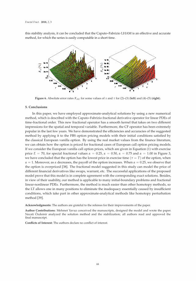
Fractal Fract. 2018, 2, 3
this stability analysis, it can be concluded that the Caputo–Fabrizio LHAM is an effective and accuratemethod, for which the series is easily computable in a short time.
Figure 6. Absolute error rates RAE for some values of x and τ for (2)–(3) (left) and (4)–(5) (right).
5. Conclusions
In this paper, we have employed approximate-analytical solutions by using a new numericalmethod, which is described with the Caputo–Fabrizio fractional derivative operator for linear PDEs oftime-fractional order. This new fractional operator has a smooth kernel that takes on two differentimpressions for the spatial and temporal variable. Furthermore, the CF operator has been extremelypopular in the last few years. We have demonstrated the efficiencies and accuracies of the suggestedmethod by applying it to the FBS option pricing models with their initial conditions satisfied bythe classical European vanilla option. By using the real market values from the finance literature,we can obtain how the option is priced for fractional cases of European call option pricing models.If we consider the European vanilla call option prices, which are given in Equation (1) with exerciseprice E = 70, for special fractional values α = 0.25, α = 0.50, α = 0.75 and α = 1.00 in Figure 3,we have concluded that the option has the lowest price in exercise time (τ = T) of the option, whenα = 1. Moreover, as α decreases, the payoff of the option increases. When α = 0.25, we observe thatthe option is overpriced [38]. The fractional model suggested in this study can model the price ofdifferent financial derivatives like swaps, warrant, etc. The successful applications of the proposedmodel prove that this model is in complete agreement with the corresponding exact solutions. Besides,in view of their usability, our method is applicable to many initial-boundary problems and fractionallinear-nonlinear PDEs. Furthermore, the method is much easier than other homotopy methods, sothe LT allows one in many positions to eliminate the inadequacy essentially caused by insufficientconditions, which take part in other approximate-analytical methods like homotopy perturbationmethod [39].
Acknowledgments: The authors are grateful to the referees for their improvements of the paper.
Author Contributions: Mehmet Yavuz conceived the manuscripts, designed the model and wrote the paper.Necati Özdemir analyzed the solution method and the stabilization; all authors read and approved thefinal manuscript.
Conflicts of Interest: The authors declare no conflict of interest.
44

Fractal Fract. 2018, 2, 3
Abbreviations
The following abbreviations are used in this manuscript:
FDE Fractional differential equationLHAM Laplace homotopy analysis methodCF Caputo–FabrizioAB Atangana–BaleanuLT Laplace transformFC Fractional calculusENSO El Niño–Southern OscillationFBSE Fractional Black–Scholes equationGFBSE Generalized fractional Black–Scholes equation
References
1. Gómez-Aguilar, J.F.; Morales-Delgado, V.F.; Taneco-Hernández, M.A.; Baleanu, D.; Escobar-Jiménez, R.F.;Al Qurashi, M.M. Analytical solutions of the electrical RLC circuit via Liouville–Caputo operators with localand non-local kernels. Entropy 2016, 18, 402, doi:10.3390/e18080402.
2. Özdemir, N.; Yavuz, M. Numerical solution of fractional Black–Scholes equation by using the multivariatePadé approximation. Acta Phys. Pol. A. 2017, 132, 1050–1053, doi:10.12693/APhysPolA.132.1050.
3. Yavuz, M.; Özdemir, N.; Okur, Y.Y. Generalized differential transform method for fractional partial differentialequation from finance. In Proceedings of the International Conference on Fractional Differentiation and itsApplications, Novi Sad, Serbia, 18–20 July 2016; pp. 778–785.
4. Alkahtani, B.S.T.; Koca, I.; Atangana, A. Analysis of a new model of H1N1 spread: Model obtained viaMittag-Leffler function. Adv. Mech. Eng. 2017, 9, 1–8, doi:10.1177/1687814017705566.
5. Momani, S.; Qaralleh, R. Numerical approximations and Padé approximants for a fractional populationgrowth model. App. Math. Model. 2007, 31, 1907–1914.
6. Hashim, I.; Abdulaziz, O.; Momani, S. Homotopy analysis method for fractional IVPs. Commun. NonlinearSci. Numer. Simul. 2009, 14, 674–684, doi:10.1016/j.cnsns.2007.09.014.
7. Evirgen, F.; Özdemir, N. Multistage Adomian decomposition method for solving NLP problems over anonlinear fractional dynamical system. J. Comput. Nonlinear Dyn. 2011, 6, doi:10.1115/1.4002393.
8. Yavuz, M.; Özdemir, N. A quantitative approach to fractional option pricing problems with decompositionseries. Konuralp J. Math. 2018, in press.
9. Elbeleze, A.A.; Kılıçman, A.; Taib, B.M. Homotopy perturbation method for fractional Black–Scholes Europeanoption pricing equations using sumudu transform. Math. Prob. Eng. 2013, 2013, 1–7, doi:10.1155/2013/524852.
10. Yavuz, M. Novel solution methods for initial boundary value problems of fractional order with conformabledifferentiation. Int. J. Opt. Control Theor. Appl. 2018, 8, 1–7, doi:10.11121/ijocta.01.2018.00540.
11. Yavuz, M.; Yaskıran, B. Approximate-analytical solutions of cable equation using conformable fractionaloperator. New Trends Math. Sci. 2017, 5, 209–219, doi:10.20852/ntmsci.2017.232.
12. Odibat, Z.; Momani, S.; Erturk, V.S. Generalized differential transform method: Application to differentialequations of fractional order. App. Math. Comput. 2008, 197, 467–477.
13. Chen, W.; Wang, S. A finite difference method for pricing European and American options under a geometricLévy process. Management 2015, 11, 241–264.
14. Turut, V.; Güzel, N. On solving partial differential equations of fractional order by using the variationaliteration method and multivariate Padé approximations. Eur. J. Pure Appl. Math. 2013, 6, 147–171.
15. Eroglu, B.I.; Avcı, D.; Özdemir, N. Optimal control problem for a conformable fractional heat conductionequation. Acta Phys. Pol. A. 2017, 132, 658–662, doi:10.12693/APhysPolA.132.658.
16. Evirgen, F. Conformable fractional gradient based dynamic system for constrained optimization problem.Acta Phys. Pol. A. 2017, 132, 1066–1069, doi:10.12693/APhysPolA.132.1066.
17. Hu, Y.; Øksendal, B.; Sulem, A. Optimal consumption and portfolio in a Black–Scholes market driven byfractional Brownian motion. Infin. Dimens. Anal. Quantum Prob. Relat. Top. 2003, 6, 519–536.
18. Özdemir, N.; Agrawal, O.P.; Karadeniz, D.; Iskender, B.B. Analysis of an axis-symmetric fractionaldiffusion-wave problem. J. Phys. A Math. Theor. 2009, 42, 355208.
45

Fractal Fract. 2018, 2, 3
19. Caputo, M.; Fabrizio, M. A new definition of fractional derivative without singular kernel. Prog. Fract.Differ. Appl. 2015, 1, 1–13, doi:10.12785/pfda/010201.
20. Atangana, A.; Alkahtani, B.S.T. New model of groundwater flowing within a confine aquifer: Application ofCaputo–Fabrizio derivative. Arab. J. Geosci. 2016, 9, 1–8, doi:10.1007/s12517-015-2060-8.
21. Singh, J.; Kumar, D.; Nieto, J.J. Analysis of an El Nino-Southern Oscillation model with a new fractionalderivative. Chaos Solitons Fractals 2017, 99, 109–115, doi:10.1016/j.chaos.2017.03.058.
22. Singh, J.; Kumar, D.; Nieto, J.J. Application of Caputo–Fabrizio derivatives to mhd free convection flow ofgeneralized Walters’-B fluid model. Eur. Phys. J. Plus 2016, 131, 377, doi:10.1140/epjp/i2016-16377-x.
23. Morales-Delgado, V.F.; Gómez-Aguilar, J.F.; Yépez-Martínez, H.; Baleanu, D.; Escobar-Jimenez, R.F.;Olivares-Peregrino, V.H. Laplace homotopy analysis method for solving linear partial differential equationsusing a fractional derivative with and without kernel singular. Adv. Differ. Equ. 2016, 2016, 164,doi:10.1186/s13662-016-0891-6.
24. Sheikh, N.A.; Ali, F.; Saqib, M.; Khan, I.; Jan, S.A.A.; Alshomrani, A.S.; Alghamdi, M.S. Comparison andanalysis of the Atangana–Baleanu and Caputo–Fabrizio fractional derivatives for generalized Casson fluidmodel with heat generation and chemical reaction. Res. Phys. 2017, 7, 789–800, doi:10.1016/j.rinp.2017.01.025.
25. Koca, I.; Atangana, A. Solutions of Cattaneo–Hristov model of elastic heat diffusion with Caputo–Fabrizioand Atangana–Baleanu fractional derivatives. Therm. Sci. 2017, 21, 2299–2305, doi:10.2298/TSCI160209103K.
26. Hristov, J. Steady-state heat conduction in a medium with spatial non-singular fading memory: Derivationof Caputo–Fabrizio space-fractional derivative with Jeffrey’s kernel and analytical solutions. Therm. Sci.2017, 21, 827–839, doi:10.2298/TSCI160229115H.
27. Alkahtani, B.S.T.; Atangana, A. Controlling the wave movement on the surface of shallow waterwith the Caputo–Fabrizio derivative with fractional order. Chaos Solitons Fractals 2016, 89, 539–546,doi:10.1016/j.chaos.2016.03.012.
28. Alkahtani, B.S.T.; Atangana, A. Analysis of non-homogeneous heat model with new trend of derivative withfractional order. Chaos Solitons Fractals 2016, 89, 566–571, doi:10.1016/j.chaos.2016.03.027.
29. Hristov, J. Transient heat diffusion with a non-singular fading memory: From the Cattaneo constitutiveequation with Jeffrey’s kernel to the Caputo–Fabrizio time-fractional derivative. Therm. Sci. 2016, 20, 757–762,doi:10.2298/TSCI160112019H.
30. Atangana, A.; Koca, I. On the new fractional derivative and application to nonlinear Baggs and Freedmanmodel. J. Nonlinear Sci. Appl. 2016, 9, 2467–2480.
31. Ghandehari, M.A.M.; Ranjbar, M. European option pricing of fractional Black–Scholes model with newLagrange multipliers. Comput. Methods Differ. Equ. 2014, 2, 1–10.
32. Yerlikaya-Özkurt, F.; Vardar-Acar, C.; Yolcu-Okur, Y.; Weber, G.W. Estimation of the Hurst parameterfor fractional Brownian motion using the CMARS method. J. Comput. Appl. Math. 2014, 259, 843–850,doi:10.1016/j.cam.2013.08.001.
33. Black, F.; Scholes, M. The pricing of options and corporate liabilities. J. Political Econ. 1973, 81, 637–654.34. Wilmott, P.; Howison, S.; Dewynne, J. The Mathematics of Financial Derivatives: A Student Introduction;
Cambridge University Press: Cambridge, UK, 1995.35. Ahmed, E.; Abdusalam, H.A. On modified Black–Scholes equation. Chaos Solitons Fractals 2004, 22, 583–587,
doi:10.1016/j.chaos.2004.02.018.36. Cen, Z.; Le, A. A robust and accurate finite difference method for a generalized Black–Scholes equation.
J. Comput. Appl. Math. 2011, 235, 3728–3733, doi:10.1016/j.cam.2011.01.018.37. Meng, L.; Wang, M. Comparison of Black–Scholes formula with fractional Black–Scholes formula in
the foreign exchange option market with changing volatility. Asia-Pac. Finan Markets 2010, 17, 99–111,doi:10.1007/s10690-009-9102-8.
38. Yavuz, M.; Özdemir, N. A different approach to the European option pricing model with new fractionaloperator. Math. Model. Nat. Phenom. 2018, in press, doi:10.1051/mmnp/2018009.
39. Madani, M.; Fathizadeh, M.; Khan, Y.; Yildirim, A. On the coupling of the homotopy perturbation methodand Laplace transformation. Math. Comput. Model. 2011, 53, 1937–1945, doi:10.1016/j.mcm.2011.01.023.
c© 2018 by the authors. Licensee MDPI, Basel, Switzerland. This article is an open accessarticle distributed under the terms and conditions of the Creative Commons Attribution(CC BY) license (http://creativecommons.org/licenses/by/4.0/).
46

fractal and fractional
Article
Fractional Derivatives with the Power-Law and theMittag–Leffler Kernel Applied to the NonlinearBaggs–Freedman Model
José Francisco Gómez-Aguilar 1,* ID and Abdon Atangana 2
1 CONACyT-Tecnológico Nacional de México/CENIDET, Interior Internado Palmira S/N, Col. Palmira,C.P. 62490 Cuernavaca, Morelos, Mexico
2 Institute for Groundwater Studies, Faculty of Natural and Agricultural Sciences, University of the Free State,Bloemfontein 9300, South Africa; [email protected]
* Correspondence: [email protected]; Tel.: +52-777-362-7770
Received: 20 November 2017; Accepted: 7 February 2018; Published: 9 February 2018
Abstract: This paper considers the Freedman model using the Liouville–Caputo fractional-orderderivative and the fractional-order derivative with Mittag–Leffler kernel in the Liouville–Caputosense. Alternative solutions via Laplace transform, Sumudu–Picard and Adams–Moulton ruleswere obtained. We prove the uniqueness and existence of the solutions for the alternative model.Numerical simulations for the prediction and interaction between a unilingual and a bilingualpopulation were obtained for different values of the fractional order.
Keywords: Freedman model; Liouville–Caputo derivative; Atangana–Baleanu derivative; fixedpoint theorem
1. Introduction
Interactions between groups that speak different languages are occurring continuously in severalcountries in the world due to globalization and cultural openness. Multilingualism is the use of morethan one language, either by an individual speaker or by a community of speakers. A mathematicalmodel portraying the interaction dynamics of a population considering bilingual components anda monolingual component was proposed in [1,2]. Baggs in [2] studied the condition under which thebilingual component could persist and conditions under which it could become extinct. The weaknessof these models is that they do not take into account the degree of interest in time and also thememory of the interaction, meaning the recall of the original meeting or interaction or contactup to a particular period of time in the present. Fractional calculus is one of the most powerfulmathematical tools used in recent decades to model real-world problems in many fields, such as science,technology and engineering. The Liouville–Caputo fractional derivative involves the power-lawfunction. The Liouville–Caputo fractional-order derivative allows usual initial conditions when playingwith the integral transform, for instance the Laplace transform [3–5]. Recently, Abdon Atangana andDumitru Baleanu proposed two fractional-order operators involving the generalized Mittag–Lefflerfunction. The generalized Mittag–Leffler function was introduced in the literature to improve thelimitations posed by the power-law [6–12]. The two-parametric, three-parametric, four-parametricand multiple Mittag–Leffler functions were presented by Wiman, Prabhakar, Shukla and Srivastavain [13–18]. The kernel used in Atangana–Baleanu fractional differentiation appears naturally in severalphysical problems as generalized exponential decay and as a power-law asymptotic for a very largetime [19–24]. The choice of this derivative is motivated by the fact that the interaction is not local,but global, and also, the trend observed in the field does not follow the power-law. The generalized
Fractal Fract. 2018, 2, 10 47 www.mdpi.com/journal/fractalfract

Fractal Fract. 2018, 2, 10
Mittag–Leffler function completely induced the effect of memory, which is very important in thenonlinear Baggs–Freedman model.
Atangana and Koca in [25] studied the nonlinear Baggs and Freedman model. Starting from theinteger-order Freedman model presented by [25], we have:
Dtx1 = (A1 − M1 − F1)x1(t)− L1x21(t)− α · x1(t)x2(t)
1+x1(t)+ G1 A2x2(t),
Dtx2 = (A2 − M2 − F2)x2(t)− L2x22(t) + α · x1(t)x2(t)
1+x1(t)− G1 A2x2(t),
(1)
where 0 < Ai, Mi, |Fi| ≤ 1 are the birth, death and emigration parameters for i ∈ [1, 2]. 0 < G1 ≤ 1is the infant language acquisition parameter, that proportion of births in the x2 population raisedunilingually. 0 < α ≤ 1 is the non-infant language acquisition rate, the proportion of x1 learning the x2
language per unit time after infancy. The term α · x1(t)x2(t)1+x1(t)
describes that part of population x1 lost tox2 due to virtual predation on the part of x2 [26].
The aim of this work is to obtain alternative representations of the Freedman model consideringLiouville–Caputo and Atangana–Baleanu–Caputo fractional derivatives. The paper is organized asfollows: Section 2 introduces the fractional operators. Alternative representations of the Freedmanmodel are shown in Section 3. Finally, in Section 4, we conclude the manuscript.
2. Fractional Operators
The Liouville–Caputo fractional-order derivative of order γ is defined by [27]:
Ca Dγ
t { f (t)} =1
Γ(1 − γ)
∫ t
af (θ)(t − θ)−γdθ, 0 < γ ≤ 1. (2)
The Laplace transform to Liouville–Caputo fractional-order derivative gives [27]:
L [Ca Dγt f (t)] = SγF(S)−
m−1
∑k=0
Sγ−k−1 f (k)(0). (3)
The Atangana–Baleanu–Caputo fractional-order derivative is defined as follows [19–22,24]:
ABCa Dγ
t { f (t)} =B(γ)1 − γ
∫ t
af (θ)Eγ
[− γ
1 − γ(t − θ)γ
]dθ, 0 < γ ≤ 1, (4)
where B(β) = B(0) = B(1) = 1 is a normalization function and Eγ is the Mittag–Leffler function [6–12].The Mittag–Leffler kernel is a combination of both the exponential-law and power-law. For thisfractional derivative, we have at the same time the power-law and the stretched exponential as thewaiting time distribution.
The Laplace transform of Equation (4) is defined as follows:
L [ABCa Dγ
t f (t)](s) = B(γ)1−γ L
[ ∫ ta f (θ)Eγ
[− γ
(t−θ)γ
1−γ
]dθ]
= B(γ)1−γ
sγL [ f (t)](s)−sγ−1 f (0)sγ+ γ
1−γ.
(5)
The Sumudu transform is derived from the classical Fourier integral [28]. The Sumudu transformof Equation (4) is defined as:
ST{
ABCa Dγ
t f (t)}=
B(γ)1 − γ
(γΓ(γ + 1)Eγ
(− 1
1 − γuγ))
× [ST( f (t))− f (0)]. (6)
48

Fractal Fract. 2018, 2, 10
The Atangana–Baleanu fractional integral of order γ of a function f (t) is defined as:
ABa Iγ
t f (t) =1 − γ
B(γ)f (t) +
γ
B(γ)Γ(γ)
∫ t
0f (s)(t − s)γ−1ds. (7)
3. Freedman Model
In this section, we obtain alternative representations of the Freedman model consideringthe Liouville–Caputo fractional derivative, and the special solution is obtained using a Laplacetransform method.
3.1. Freedman Model with the Power-Law Kernel
Considering Equation (2), the modified Freedman model with the power-law kernel is given as:
C0 D
γt x1(t) = (A1 − M1 − F1)x1(t)− L1x2
1(t)− α · x1(t)x2(t)1+x1(t)
+ G1 A2x2(t),C0 D
γt x2(t) = (A2 − M2 − F2)x2(t)− L2x2
2(t) + α · x1(t)x2(t)1+x1(t)
− G1 A2x2(t),(8)
where 0 < γ ≤ 1 is the fractional order, x1(t) represents the interaction of the majority unilingualpopulation and x2(t) is a bilingual population.
Applying the Laplace transform operator (3) and the inverse Laplace transform on both sides ofEquation (8), we obtain:
x1(t) = x1(0) +L −1{
1sγ L
[(A1 − M1 − F1)x1(t)− L1x2
1(t)− αx1(t)x2(t)1+x1(t)
+ G1 A2x2(t)](s)}(t),
x2(t) = x2(0) +L −1{
1sγ L
[(A2 − M2 − F2)x2(t)− L2x2
2(t) + αx1(t)x2(t)1+x1(t)
− G1 A2x2(t)](s)}(t).
(9)
The following iterative formula is then proposed:
x1(n)(t) = L −1{
1sγ L
[(A1 − M1 − F1)x1(n−1)(t)− L1x2
1(n−1)(t)
−αx1(n−1)(t)x2(n−1)(t)
1+x1(n−1)(t)+ G1 A2x2(n−1)(t)
](s)}(t),
x2(n)(t) = L −1{
1sγ L
[(A2 − M2 − F2)x2(n−1)(t)− L2x2
1(n−1)(t)
+αx1(n−1)(t)x2(n−1)(t)
1+x1(n−1)(t)− G1 A2x2(n−1)(t)
](s)}(t),
(10)
where,x1(0)(t) = x1(0); x2(0)(t) = x2(0), (11)
where the approximate solution is assumed to be obtained as a limit when “n” tend to infinity:
x1(t) = limn→∞
x1(n)(t); x2(t) = limn→∞
x2(n)(t). (12)
3.2. Stability Analysis of the Iteration Method
Theorem 1. We demonstrate that the recursive method given by Equation (10) is stable.
Proof. It is possible to find two positive constants Y and Z such that, for all:
0 ≤ t ≤ T ≤ ∞, ||x1(t)|| < Y and ||x1(t)|| < Z. (13)
Now, we consider a subset of C2((a, b)(0, T)) defined by:
H ={
ϕ : (a, b)(0, T) → H,1
Γ(γ)
∫(t − ϕ)γ−1v(ϕ)u(ϕ)dϕ < ∞
}, (14)
49

Fractal Fract. 2018, 2, 10
we now consider the operator φ defined as:
φ(x1, x2) =
⎧⎨⎩ (A1 − M1 − F1)x1(t)− L1x21(t)− α · x1(t)x2(t)
1+x1(t)+ G1 A2x2(t),
(A2 − M2 − F2)x2(t)− L2x22(t) + α · x1(t)x2(t)
1+x1(t)− G1 A2x2(t).
Then:
=
⎧⎪⎪⎪⎪⎪⎪⎨⎪⎪⎪⎪⎪⎪⎩
< φ(x1, x2)− φ(X1, X2), φ(x1 − X1, x2 − X2) >,< (A1 − M1 − F1)(x1(t)− X1(t))− L1(x1(t)− X1(t))2
−α · (x1(t)−X1(t))(x2(t)−X2(t))1+(x1(t)−X1(t))
+ G1 A2(x2(t)− X2(t)) >,
< (A2 − M2 − F2)(x2(t)− X2(t))− L2(x1(t)− X2(t))2
+α · (x1(t)−X1(t))(x2(t)−X2(t))1+(x1(t)−X1(t))
− G1 A2(x2(t)− X2(t)) >,
where,x1(t) �= X1(t), and x2(t) �= X2(t). (15)
Applying the absolute value on both sides, we have:
< φ(x1, x2)− φ(X1, X2), φ(x1 − X1, x2 − X2) >,
=
⎧⎪⎪⎪⎪⎪⎪⎨⎪⎪⎪⎪⎪⎪⎩
{(A1 − M1 − F1)− L1||x1(t)− X1(t)||
−α · ||x2(t)−X2(t)||1+||x1(t)−X1(t)||2 + G1 A2
||x2(t)−X2(t)||||x1(t)−X1(t)||
}||x1(t)− X1(t)||2,{
(A2 − M2 − F2)− L2||x2(t)− X2(t)||+α · ||x1(t)−X1(t)||
1+||x1(t)−X1(t)||2 − G1 A2
}||x2(t)− X2(t)||2.
(16)
Then,< φ(x1, x2)− φ(X1, X2), φ(x1 − X1, x2 − X2) >,
<
⎧⎪⎪⎪⎪⎪⎪⎨⎪⎪⎪⎪⎪⎪⎩
{(A1 − M1 − F1) + L1||x1(t)− X1(t)||
+α · ||x2(t)−X2(t)||1+||x1(t)−X1(t)||2 + G1 A2
||x2(t)−X2(t)||||x1(t)−X1(t)||
}||x1(t)− X1(t)||2,{
(A2 − M2 − F2) + L2||x2(t)− X2(t)||+α · ||x1(t)−X1(t)||
1+||x1(t)−X1(t)||2 + G1 A2
}||x2(t)− X2(t)||2,
(17)
where,< φ(x1, x2)− φ(X1, X2), φ(x1 − X1, x2 − X2) >,
<
{M||x1(t)− X1(t)||2,N||x2(t)− X2(t)||2,
(18)
with:
M = (A1 − M1 − F1) + L1||x1(t)− X1(t)||+ α · ||x2(t)− X2(t)||1 + ||x1(t)− X1(t)||2
+ G1 A2||x2(t)− X2(t)||||x1(t)− X1(t)||
,
and:
N = (A2 − M2 − F2) + L2||x2(t)− X2(t)||+ α · ||x1(t)− X1(t)||1 + ||x1(t)− X1(t)||2
+ G1 A2. (19)
Furthermore, if we consider a given non-null vector (x1, x2), then using the some routine as theabove case, we obtain:
< φ(x1, x2)− φ(X1, X2), φ(x1 − X1, x2 − X2) >,
<
{M||x1(t)− X1(t)||||x1(t)||,N||x2(t)− X2(t)||||x2(t)||,
(20)
50

Fractal Fract. 2018, 2, 10
From the results obtained in Equations (18) and (20), we conclude that the iterative method usedis stable. This complete the proof.
Now, we consider the Adams method [29,30] to solve the system given by Equation (8). The basicidea of the n-step Adams–Bashforth method is to use a polynomial interpolation for f (t, y(t)) passingthrough n points: (ti, fi), (ti−1, fi−1), ..., (ti−n+1, fi−n+1). Correspondingly, the n-step Adams–Moultonmethod uses a polynomial interpolation for f (t, y(t)) passing through n + 1 points: (ti+1, fi+1),(ti, fi), ..., (ti−n, fi−n).
The fractional Adams method is derived as follows [30]:
f Pk+1 =
n−1∑
j=0
tjk+1j!
f (j)0 +
1Γ(γ)
k∑
j=0bj,k+1g(tj, f j),
fk+1 =n−1∑
j=0
tjk+1j!
f (j)0 +
1Γ(γ)
(k∑
j=0aj,k+1g(tj, f j) + ak+1,k+1g(tk+1, f P
k+1)
),
(21)
where,
aj,k+1 =hγ
γ(γ + 1)·
⎧⎪⎨⎪⎩(kγ+1 − (k − γ)(k + 1)γ) j = 0,((k − j + 2)γ+1 + (k − j)γ+1 − 2(k − j + 1)γ+1) 1 ≤ j ≤ k,1 j = k + 1,
bj,k+1 =hγ
γ((k + 1 − j)γ − (k − j)γ), j = 0, 1, 2, ..., k.
(22)
Following this procedure, we can propose a numerical solution for System (8) using the Adamsmethod (21) as follows:
x1(t) =n−1∑
k=0x1(0)(k)
tk
k!+
1Γ(γ)
t∫0(t − u)γ−1
[(A1 − M1 − F1)x1(u)− L1x2
1(u)− α · x1(u)x2(u)1+x1(u)
+ G1 A2x2(u)]du,
x2(t) =n−1∑
k=0x2(0)(k)
tk
k!+
1Γ(γ)
t∫0(t − u)γ−1
[(A2 − M2 − F2)x2(u)− L2x2
2(u) + α · x1(u)x2(u)1+x1(u)
− G1 A2x2(u)]du.
(23)
3.3. Freedman Model with the Mittag–Leffler Kernel
Considering Equation (4), the modified Freedman model is given as:
ABC0 Dγ
t x1(t) = (A1 − M1 − F1)x1(t)− L1x21(t)− α · x1(t)x2(t)
1+x1(t)+ G1 A2x2(t),
ABC0 Dγ
t x2(t) = (A2 − M2 − F2)x2(t)− L2x22(t) + α · x1(t)x2(t)
1+x1(t)− G1 A2x2(t),
(24)
where 0 < γ ≤ 1 is the fractional order, x1(t) represents the interaction of the majority unilingualpopulation and x2(t) is a bilingual population.
Now, we obtain an alternative solution using an iterative scheme. The technique involves couplingthe Sumudu transform and its inverse. The Sumudu transform is an integral transform similar tothe Laplace transform, introduced by Watugala to solve differential equations [28–32]. Applying theSumudu transform (6) and the inverse Sumudu transform on both sides of the system (24) yields:
x1(t) = x1(0) + ST−1{
1−γ
B(γ)γΓ(γ+1)Eγ
(− 1
1−γ uγ
) · ST[(A1 − M1 − F1)x1(t)− L1x2
1(t)− αx1(t)x2(t)1+x1(t)
+ G1 A2x2(t)]}
,
x2(t) = x2(0) + ST−1{
1−γ
B(γ)γΓ(γ+1)Eγ
(− 1
1−γ uγ
) · ST[(A2 − M2 − F2)x2(t)− L2x2
2(t) + αx1(t)x2(t)1+x1(t)
− G1 A2x2(t)]}
.(25)
51

Fractal Fract. 2018, 2, 10
The following recursive formula for Equation (25) is obtained:
x1(n+1)(t) = x1(n)(0) + ST−1{
1−γ
B(γ)γΓ(γ+1)Eγ
(− 1
1−γ uγ
)·ST[(A1 − M1 − F1)x1(n)(t)− L1x2
1(n)(t)
−αx1(n)(t)x2(n)(t)
1+x1(n)(t)+ G1 A2x2(n)(t)
]},
x2(n+1)(t) = x1(n)(0) + ST−1{
1−γ
B(γ)γΓ(γ+1)Eγ
(− 1
1−γ uγ
)·ST[(A2 − M2 − F2)x2(n)(t)− L2x2
2(n)(t)
+αx1(n)(t)x2(n)(t)
1+x1(n)(t)− G1 A2x2(n)(t)
]},
(26)
and the solution of Equation (26) is provided by:
x1(t) = limn→∞
x1(n)(t); x2(t) = limn→∞
x2(n)(t). (27)
3.4. Stability Analysis of the Iteration Method
Now, we provide in detail the stability analysis of this method and show the uniqueness of the specialsolutions using the fixed point theory and properties of the inner product and the Hilbert space, respectively.
Let (X, | · |) be a Banach space and Ha self-map of X. Let zn+1 = g(H, zn) be a particular recursiveprocedure. The following conditions must be satisfied for zn+1 = Hzn.
1. The fixed point set of H has at least one element.2. zn converges to a point P ∈ F(H).3. limn→∞ xn(t) = P.
Property 1. Let (X, | · |) be a Banach space and Ha self-map of X satisfying:
||Hx − Hz|| ≤ η||X − Hx||+ η||x − z||, (28)
for all x, z ∈ X, where 0 ≤ η, 0 ≤ η < 1. Suppose that H is Picard H-stable.
Considering the following recursive formula, we have:
x1(n+1)(t) = x1(n)(0) + S−1{
1−γ
B(γ)γΓ(γ+1)Eγ
(− 1
1−γ uγ
)·S[(A1 − M1 − F1)x1(n)(t)− L1x2
1(n)(t)
−αx1(n)(t)x2(n)(t)
1+x1(n)(t)+ G1 A2x2(n)(t)
]},
x2(n+1)(t) = x2(n)(0) + S−1{
1−γ
B(γ)γΓ(γ+1)Eγ
(− 1
1−γ uγ
)·S[(A2 − M2 − F2)x2(n)(t)− L2x2
2(n)(t)
+αx1(n)(t)x2(n)(t)
1+x1(n)(t)− G1 A2x2(n)(t)
]},
(29)
where:1 − γ
B(γ)γΓ(γ + 1)Eγ
(− 1
1−γ uγ) , (30)
correspond to the fractional Lagrange multiplier.
52

Fractal Fract. 2018, 2, 10
Theorem 2. Let K be a self-map defined as:
K[x1(n+1)(t)] = x1(n+1)(t) = x1(n)(t) + S−1{
1−γ
B(γ)γΓ(γ+1)Eγ
(− 1
1−γ uγ
)·S[(A1 − M1 − F1)x1(n)(t)− L1x2
1(n)(t)− αx1(n)(t)x2(n)(t)
1+x1(n)(t)+ G1 A2x2(n)(t)
]},
K[x2(n+1)(t)] = x2(n+1)(t) = x2(n)(t) + S−1{
1−γ
B(γ)γΓ(γ+1)Eγ
(− 1
1−γ uγ
)·S[(A2 − M2 − F2)x2(n)(t)− L2x2
2(n)(t) + αx1(n)(t)x2(n)(t)
1+x1(n)(t)− G1 A2x2(n)(t)
]},
(31)
is K-stable in L1(a, b) if:
1 + (A1 − M1 − F1) f (γ)− L1||x1(n)(t) + x1(m)(t)||d(γ)− αεβ+ε+θ
ηρ ω(γ) + G1 A2k(γ) < 1,
1 + (A2 − M2 − F2)i(γ)− L2||x2(n)(t) + x2(m)(t)||r(γ) + αεβ+ε+θ
ηρ s(γ)− G1 A2o(γ) < 1,(32)
where f (γ), d(γ), ω(γ), k(γ), i(γ), r(γ), s(γ) and o(γ) are functions from:
S−1
{1 − γ
B(γ)γΓ(γ + 1)Eγ
(− 1
1−γ uγ)S
}. (33)
Proof. The proof consists of showing that K has a fixed point. To achieve this, we consider:
K[x1(n+1)(t)]− K[x1(m+1)(t)] = x1(n)(0)− x1(m)(0) + S−1
{1−γ
B(γ)γΓ(γ+1)Eγ
(− 1
1−γ uγ
)·S[((A1 − M1 − F1)x1(n)(t)− (A1 − M1 − F1)x1(m)(t))− (L1x2
1(n)(t) + L1x21(m)(t))
−(
α(x1(n)(t)−x1(m)(t))·(x2(n)(t)−x2(m)(t))
1+(x1(n)(t)−x1(m)(t)
)+ G1 A2(x2(n)(t)− x2(m)(t))
]},
and:
K[x2(n+1)(t)]− K[x2(m+1)(t)] = x2(n)(0)− x2(m)(0) + S−1
{1−γ
B(γ)γΓ(γ+1)Eγ
(− 1
1−γ uγ
)·S[((A2 − M2 − F2)x2(n)(t)− (A2 − M2 − F2)x2(m)(t))− (L2x2
2(n)(t) + L2x22(m)(t))
+
(α(x1(n)(t)−x1(m)(t))·(x2(n)(t)−x2(m)(t))
1+(x1(n)(t)−x1(m)(t)
)− G1 A2(x2(n)(t)− x2(m)(t))
]}.
(34)
Using the properties of the norm and considering the triangular inequality, we get:
||K[x1(n)(t)]− K[x1(m)(t)]|| ≤ ||x1(n)(t)− x1(m)(t)||+ S−1
{1−γ
B(γ)γΓ(γ+1)Eγ
(− 1
1−γ uγ
)·S[((A1 − M1 − F1)x1(n)(t)− (A1 − M1 − F1)x1(m)(t))− (L1x2
1(n)(t) + L1x21(m)(t))
+
(α(x1(n)(t)−x1(m)(t))·(x2(n)(t)−x2(m)(t))
1+(x1(n)(t)−x1(m)(t)
)− G1 A2(x2(n)(t)− x2(m)(t))
]}.
(35)
we consider that the solutions play the some role, i.e., ||x2(n)(t)− x2(m)(t)|| ∼= ||x1(n)(t)− x1(m)(t)||.
53

Fractal Fract. 2018, 2, 10
Using the linearity of the inverse Sumudu transform, we get:
||K[x1(n)(t)]− K[x1(m)(t)]|| ≤ ||x1(n)(t)− x1(m)(t)||
+S−1
{1−γ
B(γ)γΓ(γ+1)Eγ
(− 1
1−γ uγ
)S(||(A1 − M1 − F1)[x1(n)(t)− x1(m)(t)]||
)}
+S−1
{1−γ
B(γ)γΓ(γ+1)Eγ
(− 1
1−γ uγ
)S(|| − L1[x2
1(n)(t)− x21(m)(t)]||
)}
+S−1
{1−γ
B(γ)γΓ(γ+1)Eγ
(− 1
1−γ uγ
)·S(∣∣∣∣∣∣∣∣∣∣− α
(x1(m)(t)(x1(n)(t))((x1(n)(t)−x1(m)(t))1+(x1(n)(t)(1+x1(m)(t))
+x1(n)(t)(x1(n)(t)−x1(m)(t))+x2(n)(t)(x2(n)(t)−x1(m)(t))
1+(x1(n)(t)(1+x1(m)(t))
∣∣∣∣∣∣∣∣∣∣)}
+S−1
{1−γ
B(γ)γΓ(γ+1)Eγ
(− 1
1−γ uγ
)S||G1 A2[x1(n)(t)− x1(m)(t))]||}
.
(36)
Since x1(n)(t) and x1(m)(t) are bounded, we can find the following positive constants, ε, β, θ, η
and ρ such that for all t:
||x1(n)(t)|| ≤ ε, ||x1(m)(t)|| ≤ β, ||1 + x1(n)(t)|| ≤ ρ,||x2(n)(t)|| ≤ θ, ||1 + x1(m)(t)|| ≤ η, (n, m) ∈ N × N.
(37)
Considering Equations (36) and (37), we obtain:
||K[x1(n)(t)]− K[x1(m)(t)]|| ≤ ||x1(n)(t)− x1(m)(t)||
·(
1 + (A1 − M1 − F1) f (γ)− L1||x1(n)(t) + x1(m)(t)||d(γ)− αεβ+ε+θ
ηρ ω(γ) + G1 A2k(γ)
),
(38)
and:
||K[x2(n)(t)]− K[x2(m)(t)]|| ≤ ||x2(n)(t)− x2(m)(t)||
·(
1 + (A2 − M2 − F2)i(γ)− L2||x2(n)(t) + x2(m)(t)||r(γ) + αεβ+ε+θ
ηρ s(γ)− G1 A2o(γ)
),
(39)
where f (γ), d(γ), ω(γ), k(γ), i(γ), r(γ), s(γ) and o(γ) are functions from (33).We next show that K satisfies Property 1. Consider Equations (38) and (39), yielding:
η(0, 0), η =
{1 + (A1 − M1 − F1) f (γ)− L1||x1(n)(t) + x1(m)(t)||d(γ)− α
εβ+ε+θηρ ω(γ) + G1 A2k(γ),
1 + (A2 − M2 − F2)i(γ)− L2||x2(n)(t) + x2(m)(t)||r(γ) + αεβ+ε+θ
ηρ s(γ)− G1 A2o(γ),
We conclude that K is Picard K-stable.
3.5. Uniqueness of the Special Solution
Theorem 3. We consider the Hilbert space H = L2((a, b) × (0, k)) that can be defined as the set ofthose functions:
v : (a, b)× [0, T] → R,∫ ∫
uvdudv < ∞. (40)
54

Fractal Fract. 2018, 2, 10
We now consider the following operator:
η(0, 0), η =
⎧⎨⎩ (A1 − M1 − F1)x1(t)− L1x21(t)− α
x1(t)x2(t)1+x1(t)
+ G1 A2x2(t),
(A2 − M2 − F2)x2(t)− L2x22(t) + α
x1(t)x2(t)1+x1(t)
− G1 A2x2(t),
Proof. We prove that the inner product of:
(T(x11(t)− x12(t), x21(t)− x22(t), (ω1, ω2)), (41)
where (x11(t) − x12(t)), x21(t) − x22(t) are special solutions of the system. We can assume that(x11(t)− x12(t)) ∼= x21(t)− x22(t).
Using the relationship between the norm and the inner function, we get:
((A1 − M1 − F1)(x11(t)− x12(t))− L1(x11(t)− x12(t))2 − α
(x11(t)−x12(t))(x21(t)−x22(t))1+(x11(t)−x12(t))
+ G1 A2(x21(t)− x22(t)), ω1
)≤ (A1 − M1 − F1)||x11 − x12||||ω1||+ L1||x11 − x12||2||ω1||+ α
||x11(t)−x12(t)||2||1+(x11(t)−x12(t))|| ||ω1||+ G1 A2||x11 − x12||||ω1||
(42)
and:((A2 − M2 − F2)(x21(t)− x22(t))− L2(x21(t)− x22(t))2 + α
(x11(t)−x12(t))(x21(t)−x22(t))1+(x11(t)−x12(t))
+ G1 A2(x22(t)− x21(t)), ω2
)≤ (A2 + M2 − F2)||x21 − x22||||ω2||+ L2||x22 − x21||2||ω2||+ α
||x22(t)−x21(t)||2||1+(x22(t)−x21(t))|| ||ω2||+ G1 A2||x22 − x21||||ω2||;
(43)
for large number m and n, both solutions converge to the exact solution; if η = ||X1 − X11||, ||X1 − X12||and ν = ||x2 − x21||, ||x2 − x22||, we have:
η <λn
2
((A1 − M1 − F1) + L1||x11(t)− x12(t)||+ α
||x11(t)−x12(t)||1+x11(t)−x12(t)
+ G1 A2
)∣∣∣∣∣∣∣∣∣∣ω1
∣∣∣∣∣∣∣∣∣∣, (44)
and:ν <
λm
2
((A2 + M2 − F2) + L2||x22(t)− x21(t)||+ α
||x22(t)−x21(t)||1−(x22(t)−x21(t))
+ G1 A2
)∣∣∣∣∣∣∣∣∣∣ω2
∣∣∣∣∣∣∣∣∣∣, (45)
where λn and λm are two very small positive parameters.Using the topology concept, we conclude that λn < 0 and λm < 0, where:(
(A1 − M1 − F1) + L1||x11(t)− x12(t)||+ α||x11(t)−x12(t)||1+x11(t)−x12(t)
+ G1 A2
)�= 0,(
(A2 + M2 − F2) + L2||x22(t)− x21(t)||+ α||x22(t)−x21(t)||
1−(x22(t)−x21(t))+ G1 A2
)�= 0.
(46)
This completes the proof.
Involving the Atangana–Baleanu fractional integral, we can propose a numerical solution usingthe Adams–Moulton rule:
AB0 Iγ
t [ f (tn+1)] =1 − γ
B(γ)
[ f (tn+1)− f (tn)
2
]+
γ
Γ(γ)
∞
∑k=0
[ f (tk+1)− f (tk)
2
]bγ
k , (47)
55

Fractal Fract. 2018, 2, 10
where:bγ
k = (k + 1)1−γ − (k)1−γ. (48)
Considering the above numerical scheme, we have:
x1(n+1)(t)− x1(n)(t) = xn0(1)(t) +
{1−γB(γ)
[(A1 − M1 − F1)
x1(n+1)(t)−x1(n)(t)2
−L1
( x21(n+1)(t)−x2
1(n)(t)2
)− α
(x1(n+1)(t)−x1(n)(t))(x2(n+1)(t)−x2(n)(t))2
1+(x1(n+1)(t)−x1(n)(t))+ G1 A2
( x2(n+1)−x2(n)(t)2
)]
+ γB(γ) ∑∞
k=0 bγk ·[(A1 − M1 − F1)
x1(k+1)(t)−x1(k)(t)2 − L1
( x21(k+1)(t)−x2
1(k)(t)2
)−α
(x1(k+1)(t)−x1(k)(t))(x2(k+1)(t)−x2(k)(t))2
1+(x1(k+1)(t)−x1(k)(t))− G1 A2
( x2(k+1)−x2(k)(t)2
)],
(49)
and:
x2(n+1)(t)− x2(n)(t) = xn0(2)(t) +
{1−γB(γ)
[(A2 − M2 − F2)
x2(n+1)(t)−x2(n)(t)2 −
−L2
( x22(n+1)(t)−x2
2(n)(t)2
)+ α
(x1(n+1)(t)−x1(n)(t))(x2(n+1)(t)−x2(n)(t))2
1+(x1(n+1)(t)−x1(n)(t))+ G1 A2
( x2(n+1)−x2(n)(t)2
)]
+ γB(γ) ∑∞
k=0 bγk ·[(A2 − M2 − F2)
x2(k+1)(t)−x2(k)(t)2 − L2
( x22(k+1)(t)−x2
2(k)(t)2
)−α
(x1(k+1)(t)−x1(k)(t))(x2(k+1)(t)−x2(k)(t))2
1+(x1(k+1)(t)−x1(k)(t))− G1 A2
( x2(n+1)−x2(n)(t)2
)].
(50)
The proof of existence is described in detail by Alkahtani in [20].
4. Numerical Results
Example 1. We present numerical simulations of the special solution of our model using the Adams–Moultonrule given by Equation (23) and Equations (49) and (50) for different arbitrary values of fractional order γ.We consider A1 = 0.017; A2 = 0.30; M1 = 0.06; M2 = 0.007; L1 = 0.01; L2 = 0.004; F1 = 0.3; F2 = 0.7;G1 = 0.01; α = 0.05; and initial conditions x(0) = 10; y(0) = 10, arbitrarily chosen. The simulation timeis 10 s, and the step size used in evaluating the approximate solution was h = 0.001. The numerical resultsgiven in Figures 1a–d, 2a–d, 3a–d, and 4a–d show numerical simulations of the special solution of our model asa function of time for different values of γ.
The figures show the interaction dynamics between a bilingual component and a monolingualcomponent of a population in a particular environment. These numerical results show the influence offractional order γ in the prediction between the unilingual and bilingual population.
56

Fractal Fract. 2018, 2, 10
0 0.2 0.4 0.6 0.8 10
1
2
3
4
5
6
7
8
9
10
Time
Fut
ure
inte
ract
ion
Unilingual populationBilingual population
0 2 4 6 8 101
2
3
4
5
6
7
8
9
10
Unilingual population
Bili
ngua
l pop
ulat
ion
(a) (b)
0 0.2 0.4 0.6 0.8 10
1
2
3
4
5
6
7
8
9
10
Time
Fut
ure
inte
ract
ion
Unilingual populationBilingual population
0 2 4 6 8 100
1
2
3
4
5
6
7
8
9
10
Unilingual population
Bili
ngua
l pop
ulat
ion
(c) (d)
Figure 1. Numerical simulation for the nonlinear Freedman model via Liouville–Caputo fractionaloperator. In (a,c), the prediction between the two populations for γ = 1 (classical case) and γ = 0.9.In (b,d), the interaction between the unilingual and bilingual population for γ = 1 (classical case) andγ = 0.9.
0 0.2 0.4 0.6 0.8 10
1
2
3
4
5
6
7
8
9
10
Time
Fut
ure
inte
ract
ion
Unilingual populationBilingual population
0 2 4 6 8 100
1
2
3
4
5
6
7
8
9
10
Unilingual population
Bili
ngua
l pop
ulat
ion
(a) (b)
0 0.2 0.4 0.6 0.8 10
1
2
3
4
5
6
7
8
9
10
Time
Fut
ure
inte
ract
ion
Unilingual populationBilingual population
0 2 4 6 8 100
1
2
3
4
5
6
7
8
9
10
Unilingual population
Bili
ngua
l pop
ulat
ion
(c) (d)
Figure 2. Numerical simulation for the nonlinear Freedman model via Liouville–Caputo fractionaloperator. In (a,c), the prediction between the two populations for γ = 0.8 and γ = 0.7. In (b,d), theinteraction between the unilingual and bilingual population for γ = 0.8 (classical case) and γ = 0.7.
57

Fractal Fract. 2018, 2, 10
0 0.2 0.4 0.6 0.8 10
1
2
3
4
5
6
7
8
9
10
Time
Fut
ure
inte
ract
ion
Unilingual populationBilingual population
0 2 4 6 8 101
2
3
4
5
6
7
8
9
10
Unilingual population
Bili
ngua
l pop
ulat
ion
(a) (b)
0 0.2 0.4 0.6 0.8 11
2
3
4
5
6
7
8
9
10
Time
Fut
ure
inte
ract
ion
Unilingual populationBilingual population
1 2 3 4 5 6 7 8 9 101
2
3
4
5
6
7
8
9
10
Unilingual population
Bili
ngua
l pop
ulat
ion
(c) (d)
Figure 3. Numerical simulation for the nonlinear Freedman model via Atangana–Baleanu–Caputofractional operator. In (a,c), the prediction between the two populations for γ = 1 (classical case) andγ = 0.9. In (b,d), the interaction between the unilingual and bilingual population for γ = 1 (classicalcase) and γ = 0.9.
0 0.2 0.4 0.6 0.8 11
2
3
4
5
6
7
8
9
10
Time
Fut
ure
inte
ract
ion
Unilingual populationBilingual population
1 2 3 4 5 6 7 8 9 101
2
3
4
5
6
7
8
9
10
Unilingual population
Bili
ngua
l pop
ulat
ion
(a) (b)
0 0.2 0.4 0.6 0.8 11
2
3
4
5
6
7
8
9
10
Time
Fut
ure
inte
ract
ion
Unilingual populationBilingual population
1 2 3 4 5 6 7 8 9 101
2
3
4
5
6
7
8
9
10
Unilingual population
Bili
ngua
l pop
ulat
ion
(c) (d)
Figure 4. Numerical simulation for the nonlinear Freedman model via Atangana–Baleanu–Caputofractional operator. In (a,c), the prediction between the two populations for γ = 0.8 and γ = 0.7.In (b,d), the interaction between the unilingual and bilingual population for γ = 0.8 (classical case)and γ = 0.7.
58

Fractal Fract. 2018, 2, 10
5. Conclusions
A Freedman model was considered using the fractional derivatives of the Liouville–Caputoand Atangana–Baleanu–Caputo types. The solutions of the alternative models were obtained usingan iterative scheme based on the Laplace transform and the Sumudu transform. Furthermore, weemployed the fixed point theorem to study the stability analysis of the iterative methods, and usingproperties of the inner product and the Hilbert space, the uniqueness of the special solution waspresented in detail. Additionally, special solutions via the Adams–Moulton rule were obtained for bothfractional derivatives. The results obtained using the Liouville–Caputo and Atangana–Baleanu-Caputoderivatives are exactly the same as the ordinary case. However, as γ takes values smaller than one,the results obtained become a little different, having a remarkable difference when γ < 0.9. This is dueto the kernel involved in the definitions of the fractional derivative. The computer used for obtainingthe results in this paper is an Intel Core i7, 2.6-GHz processor, 16.0 GB RAM (MATLAB R.2013a).
Acknowledgments: The authors appreciate the constructive remarks and suggestions of the anonymousreferees that helped to improve the paper. We would like to thank to Mayra Martínez for the interestingdiscussions. José Francisco Gómez Aguilar acknowledges the support provided by CONACyT: cátedrasCONACyT para jóvenes investigadores 2014. José Francisco Gómez Aguilar acknowledges the support providedby SNI-CONACyT.
Author Contributions: The analytical results were worked out by José Francisco Gómez Aguilar andAbdon Atangana. José Francisco Gómez Aguilar and Abdon Atangana wrote the paper. All authors haveread and approved the final manuscript.
Conflicts of Interest: The authors declare no conflict of interest.
References
1. Baggs, I.; Freedman, H.I. A mathematical model for the dynamics of interactions between a unilingual anda bilingual population: Persistence versus extinction. J. Math. Sociol. 1990, 16, 51–75.
2. Baggs, I.; Freedman, H.I.; Aiello, W.G. Equilibrium characteristics in models of unilingual-bilingualpopulation interactions. In Ocean Wave Mechanics, Computational Fluid Dynamics, and Mathematical Modeling;Rahman, M., Ed.; Computational Mechanics Publ.: Southampton, UK, 1990; pp. 879–886.
3. Duan, B.; Zheng, Z.; Cao, W. Spectral approximation methods and error estimates for Caputo fractionalderivative with applications to initial-value problems. J. Comput. Phys. 2016, 319, 108–128.
4. Gómez, J.F. Comparison of the Fractional Response of a RLC Network and RC Circuit. Prespacetime J. 2012, 3,736–742.
5. Ito, K.; Jin, B.; Takeuchi, T. On the sectorial property of the Caputo derivative operator. Appl. Math. Lett.2015, 47, 43–46.
6. Kochubei, A.N. General fractional calculus, evolution equations, and renewal processes. Integral Equ.Oper. Theory 2011, 71, 583–600.
7. Sandev, T.; Metzler, R.; Tomovski, Z. Velocity and displacement correlation functions for fractionalgeneralized Langevin equations. Fract. Calc. Appl. Anal. 2012, 15, 426–450.
8. Sandev, T.; Tomovski, Z.; Dubbeldam, J.L. Generalized Langevin equation with a three parameterMittag–Leffler noise. Phys. A Stat. Mech. Appl. 2011, 390, 3627–3636.
9. Eab, C.H.; Lim, S.C. Fractional generalized Langevin equation approach to single-file diffusion. Phys. A Stat.Mech. Appl. 2010, 389, 2510–2521.
10. Ahmad, B.; Nieto, J.J.; Alsaedi, A.; El-Shahed, M. A study of nonlinear Langevin equation involving twofractional orders in different intervals. Nonlinear Anal. Real World Appl. 2012, 13, 599–606.
11. Metzler, R.; Klafter, J. Subdiffusive transport close to thermal equilibrium: from the Langevin equation tofractional diffusion. Phys. Rev. E 2000, 61, 6308–6311.
12. Lutz, E. Fractional langevin equation. In Fractional Dynamics: Recent Advances; World Scientific: Singapore,2012; pp. 285–305.
13. Wiman, A. Über den Fundamentalsatz in der Teorie der Funktionen Ea(x). Acta Math. 1905, 29, 191–201.14. Prabhakar, T.R. A singular integral equation with a generalized Mittag–Leffler function in the kernel.
Yokohama Math. J. 1971, 19, 7–15.
59

Fractal Fract. 2018, 2, 10
15. Shukla, A.K.; Prajapati, J.C. On a generalization of Mittag–Leffler function and its properties. J. Math.Anal. Appl. 2007, 336, 797–811.
16. Srivastava, H.M.; Tomovski, Z. Fractional calculus with an integral operator containing a generalizedMittag–Leffler function in the kernel. Appl. Math. Comput. 2009, 211, 198–210.
17. Saxena, R.K.; Ram, J.; Vishnoi, M. Fractional differentiation and fractional integration of the generalizedMittag–Leffler function. J. Indian Acad. Math. 2010, 32, 153–162.
18. Kiryakova, V.S. Multiple (multiindex) Mittag–Leffler functions and relations to generalized fractionalcalculus. J. Comput. Appl. Math. 2000, 118, 241–259.
19. Atangana, A.; Baleanu, D. New Fractional Derivatives with Nonlocal and Non-Singular Kernel: Theory andApplication to Heat Transfer Model. Therm. Sci. 2016, 20, 763–769.
20. Alkahtani, B.S.T. Chua’s circuit model with Atangana–Baleanu derivative with fractional order.Chaos Solitons Fractals 2016, 89, 547–551.
21. Algahtani, O.J.J. Comparing the Atangana–Baleanu and Caputo-Fabrizio derivative with fractional order:Allen Cahn model. Chaos Solitons Fractals 2016, 89, 552–559.
22. Alkahtani, B.S.T. Analysis on non-homogeneous heat model with new trend of derivative with fractionalorder. Chaos Solitons Fractals 2016, 89, 566–571.
23. Gómez-Aguilar, J.F.; López-López, M.G.; Alvarado-Martínez, V.M.; Reyes-Reyes, J.; Adam-Medina, M.Modeling diffusive transport with a fractional derivative without singular kernel. Phys. A Stat. Mech. Appl.2016, 447, 467–481.
24. Atangana, A.; Koca, I. Chaos in a simple nonlinear system with Atangana–Baleanu derivatives with fractionalorder. Chaos Solitons Fractals 2016, 89, 447–454.
25. Atangana, A.; Koca, I. On the new fractional derivative and application to nonlinear Baggs and Freedmanmodel. J. Nonlinear Sci. Appl. 2016, 9, 2467–2480.
26. Wyburn, J.; Hayward, J. The future of bilingualism: an application of the Baggs and Freedman model.J. Math. Sociol. 2008, 32, 267–284.
27. Caputo, M.; Mainardi, F. A new dissipation model based on memory mechanism. Pure Appl. Geophys. 1971,91, 134–147.
28. Watugala, G.K. Sumudu transform: A new integral transform to solve differential equations and controlengineering problems. Integr. Educ. 1993, 24, 35–43.
29. Li, C.; Tao, C. On the fractional Adams method. Comput. Math. Appl. 2009, 58, 1573–1588.30. Diethelm, K.; Ford, N.J.; Freed, A.D. Detailed error analysis for a fractional Adams method. Numer. Algorithms
2004, 36, 31–52.31. Katatbeh, Q.K.; Belgacem, F.B.M. Applications of the Sumudu transform to fractional differential equations.
Nonlinear Stud. 2011, 18, 99–112.32. Bulut, H.; Baskonus, H.M.; Belgacem, F.B.M. The analytical solutions of some fractional ordinary differential
equations by Sumudu transform method. Abstr. Appl. Anal. 2013, 2013, 203875.
c© 2018 by the authors. Licensee MDPI, Basel, Switzerland. This article is an open accessarticle distributed under the terms and conditions of the Creative Commons Attribution(CC BY) license (http://creativecommons.org/licenses/by/4.0/).
60

fractal and fractional
Article
Comparison between the Second and ThirdGenerations of the CRONE Controller: Application toa Thermal Diffusive Interface Medium
Xavier Moreau 1, Roy Abi Zeid Daou 2,3,* and Fady Christophy 4
1 UMR 5218 CNRS, IMS Laboratory, University of Bordeaux, 33405 Talence Cedex, France;[email protected]
2 Biomedical Technologies Department, Faculty of Public Health, Lebanese German University, Sahel Alma,Jounieh 1200, Lebanon
3 MART Learning, Education and Research Center, Chananiir 1200, Lebanon4 Faculty of Engineering, Lebanese University, Tripoli 1300, Lebanon; [email protected]* Correspondence: [email protected] or [email protected]; Tel.: +961-3-396-099
Received: 19 December 2017; Accepted: 12 January 2018; Published: 17 January 2018
Abstract: The control of thermal interfaces has gained importance in recent years because of the highcost of heating and cooling materials in many applications. Thus, the main focus in this work is tocompare the second and third generations of the CRONE controller (French acronym of CommandeRobuste d’Ordre Non Entier), which means a non-integer order robust controller, and to synthesizea robust controller that can fit several types of systems. For this study, the plant consists of arectangular homogeneous bar of length L, where the heating element in applied on one boundary,and a temperature sensor is placed at distance x from that boundary (x is considered very smallwith respect to L). The type of material used is the third parameter, which may help in analyzingthe robustness of the synthesized controller. The originality of this work resides in controlling anon-integer plant using a fractional order controller, as, so far, almost all of the systems where theCRONE controller has been implemented were of integer order. Three case studies were defined inorder to show how and where each CRONE generation controller can be applied. These case studieswere chosen in such a way as to influence the asymptotic behavior of the open-loop transfer functionin the Black–Nichols diagram in order to point out the importance of respecting the conditions ofthe applications of the CRONE generations. Results show that the second generation performs wellwhen the parametric uncertainties do not affect the phase of the plant, whereas the third generation isthe most robust, even when both the phase and the gain variations are encountered. However, it alsohas some limitations, especially when the temperature to be controlled is far from the interface whenthe density of flux is applied.
Keywords: CRONE controller; homogeneous plan diffusive interface; semi-infinite medium;robust control
1. Introduction
The thermal application is a common application for control. It is used in several engineeringdomains as the heating/cooling of houses [1,2], the control of the temperature inside the car [3,4]or in the industrial machinery [5], and much more. In more details, the work in this field started inthe 1940s with the works of Jones [6] and a group of American electrical engineers [7]. Then, in the1950s, the researchers were more involved in the control of thermal neutron reactors [8,9] and electriccables dissipation [10,11]. These studies had increased since the end of the previous decade, when thescientists stopped focusing on the study of the material properties, and started searching for more
Fractal Fract. 2018, 2, 5 61 www.mdpi.com/journal/fractalfract

Fractal Fract. 2018, 2, 5
ecological systems to control the temperature within the building in order to reduce the oil and fuelusage [12,13].
However, the work on diffusive interfaces was launched in the late 1970s and 1980s with theworks of Kumar, who modeled the thermal boundaries near an oil plant [14]. As for the others, theyworked on the modeling of diffusive interfaces at furnaces [15], boilers [16] and some geometricshapes representing the separation medium [17,18]. In the last decade of the twentieth century, thisdomain was investigated by lots of researchers who demonstrated that the relation between theinput flux and the output temperature is of a fractional order. From among them, we can recognizethe remarkable works of Trigeassou and his team [19–21], Battablia [22,23], the CRONE team ofBordeaux university [24–26], the relevant modeling approach based on the space-fractional continuummodels [27–29], and much more.
As for the control, it was applied a long time ago, even before Christ, when Ktesibios (270 B.C.)implemented the water clocks working on feedback control [30]. The contemporary control theorywas effectively launched in the middle of the twentieth century with the remarkable work of Bode,Nichols, and Nyquist [31]. In its first years, the integer and linear order systems were treated on bothtime and frequency domains.
As for fractional theory, it is relatively an old idea that dates back to the end of the seventiethcentury, when some letters were exchanged between two well-known mathematicians at that epoch,L’Hopital and Leibnitz in which they asked each other about the meaning of a derivative of order0.5 [32]. Many mathematicians defined this type of derivative/integration as Liouville, Caputo, andRiemann [33]. Nevertheless, these calculations remained theoretical until the last quarter of thetwentieth century, when Oustaloup was the first to design a fractional control of order 3/2 to control alaser beam [34]. He was one of the first researchers to introduce the fractional calculus in engineeringdomain applications [35–38]. Due to the obtained results, many other contributions appeared fromOrtigueira [39,40], Machado [41,42], and Vinagre [43,44].
Hence, this paper will present the control of a diffusive interface medium, consisting of ahomogeneous rectangular finite rod, by the CRONE controller. The novelty of this work is thatit presents a fractional order plant that will be controlled by a fractional order controller, who willbe, for the first time, real (when applying the second generation CRONE), and in a second time, thiscontroller will be complex (by applying the third generation CRONE). Added to that, the robustnessof these controllers will be studied when varying the bar metal, the position of the point where thetemperature is to be measured, the length of the bar, and so on. Thus, three case studies will be shownin order to show the behavior of the open-loop system, and to indicate the conditions of application foreach CRONE generation. Since the objective of this paper is to point out the importance of applyingthe CRONE controller to a fractional order plant, we were not interested in comparing the performanceof this controller to other ones.
For the remaining part of this paper, we will consider that the length of the bar is much moreimportant than the position of the temperature sensor. As for the user specifications, two mainconstraints will be considered hereafter:
• A crossover frequency ωcg = 1 rad/s;• A phase margin Mφ = 3 dB;
To do so, this paper will be divided as follows: in Section 2, the homogeneous finite andrectangular bar will be presented, along with its mathematical modeling and its boundary conditions.In Section 3, the different applied controllers will be introduced; an overview of the three CRONEgenerations will also be proposed, along with the conditions of application of each generation.In Section 4, the second CRONE generation will be presented along with two case studies: the firstone shows an ideal domain of application where the phase is constant and the gain varies wheneverplant parameters change. The second case presents both phase and gain variations, and the use ofthe already synthesized controller appears to be no more robust. Hence, for this second case study,
62

Fractal Fract. 2018, 2, 5
the third generation controller will be introduced in Section 5, and a performance analysis will bepresented. At the end, Section 6 will provide a conclusion and some future works to enrich this work.
2. Plant Modeling
The homogeneous diffusive interface medium will be presented in this part. The test bench isconstituted of a rectangular homogeneous rod with a square section S. It may consist of aluminum,copper, or iron, and it is of a finite distance L, as shown in Figure 1. The characteristics of the medium,its differential equations, and the boundary conditions, along with the features of the material usedwill be proposed hereafter.
Figure 1. Representation of diffusive interface medium along with the sensors and the heating element.
2.1. Partial Differential Equations (PDE)
The input of this medium will be the density of flux ϕ(t) (which is equal to the flux φ(t) dividedby the section S of the source), whereas the output is the temperature at a location x. The partialdifferential equations of this medium are shown in system (1), where the first equation shows thetemperature value for any value of x. As for the second equation, it represents the temperaturevariation at the boundary where the heating element is applied.{
∂T(x,t)∂t = αd
∂2T(x,t)∂x2 , x > 0 , t > 0
−λ∂T(x,t)
∂x = φ(t) , x = 0 , t > 0, (1)
where αd represents the thermal diffusivity of the material, and T(x,t) represents the temperature at theposition x for time t.
In the second boundary equation, the flux is not applied, and the temperature along the bar at theinitial time (t = 0 s) is expressed by the following system:{
−λ∂T(x,t)
∂x = 0 , x = L , t > 0T(x, t) = 0 , 0 ≤ x < L , t = 0
. (2)
2.2. Plant Transfer Function
Based on the partial differential equations that represent the relation between the applied densityof flux ϕ(t) and the temperature variation T(x,t,L) within the diffusive interface medium of length L,one can deduce the transfer function H(x,s,L) that models this system (interested authors can refer tothe following references for a detailed calculation of this transfer function [45,46]). Note here that the
63

Fractal Fract. 2018, 2, 5
temperature varies with respect to the material used, the placement x of the temperature sensor, andthe length L of the rod. This transfer function H(x,s,L) is given by:
H(x, s, L) =T(x, s, L)
ϕ(s)= H0
1s0.5
1
tanh(√
sωL
) cosh(√
sωLx
)cosh
(√s
ωL
) ,
H0 =1
S ηd, ηd =
√λ ρ Cp, ωL =
αdL2 , ωLx =
αd
(L − x)2 ,
(3)
where T(x, s, L) and ϕ(s) represent the Laplace transform of T(x,t,L) and ϕ(t) respectively, ηd is thethermal effusivity, λ represents the thermal conductivity, ρ is the medium density, and Cp is themedium heat.
From Equation (3), one can notice the fractional order operator (√
s) residing in the hyperbolicaltrigonometric functions, as well as the pure semi-integrator. This can confirm, once again, the noveltyof this work by applying a fractional order control (the CRONE controller) to, most importantly,a non-integer order plant.
However, the expression of the transfer function H(x,s,L) can be reduced: in fact, as the positionof the temperature sensor is neglected with respect to the length of the bar (x << L), one can deducethat ωLx ≈ ωL. Thus, Equation (3) can be written as follows, where this latter defines the validationmodel of the system:
H(x, s, L) =T(x, s, L)
ϕ(s)= H0
1s0.5
1
tanh(√
sωL
) e−√ s
ωx , (4)
where ωx = αd/x2.
2.3. Material Characteristics
As previously proposed, three materials will be used: copper (Cop), iron (Iro), and aluminum(Alu). The last one will be considered for the nominal case. Table 1 shows the characteristics of thethree materials, along with the values of the two transitional frequencies ωL and ωx for three values ofthe length, L, and the temperature sensor position, x.
Table 1. Physical characteristics of the used materials. Alu: aluminum; Cop: copper; Iro: iron.
Materialαd ηd H0 �L (rad/s) �x (rad/s)
m2/s W·K−1·m−2·s0.5 K·s0.5·W−1 L = 0.25 m L = 0.5 m L = 1 m x = 0 cm x = 0.5 cm x = 1 cm
Cop. 117 × 10−6 3.72 × 10⁴ 0.269 19 × 10−4 4.68 × 10⁻⁴ 1.17 × 10⁻⁴ Infinite 4.68 1.17Alu. 97 × 10−6 2.41 × 10⁴ 0.416 16 × 10−4 3.88 × 10⁻⁴ 0.97 × 10⁻⁴ Infinite 3.88 0.97Iro. 23 × 10−6 1.67 × 10⁴ 0.596 3.68 × 10⁻⁴ 0.92 × 10⁻⁴ 0.23 × 10⁻⁴ Infinite 0.92 0.23
When synthesizing the controllers, two case studies will be proposed based on the values of Land x for the three material types. In the next sections, these case studies will be defined in more detail,and the plant uncertainties will be modeled.
3. CRONE Controllers Presentation
The controllers that would be used in this application are the second and third generation CRONEcontrollers. In the following, we will present each controller, and the method to synthesize it. Thetwo next sections will show the applications of the second and the third generations using twodifferent case studies. This will help the user understand the conditions in which to apply each of theCRONE generations.
64

Fractal Fract. 2018, 2, 5
The CRONE controller is the first fractional order controller developed. It was launched in 1975,and it was introduced using three generations. We will focus in this paper on the second and thirdgenerations, knowing that the first two generations were treated in previous works [47,48]. However,a brief overview over the three generations will be presented below.
The first generation Crone controller proposes to use a controller without phase variation aroundcrossover frequency ωcg. Thus, the phase margin variation only results from the plant variation. Thisstrategy has to be used when frequency ωcg is within a frequency range where the plant phase isconstant. In this range, the plant variations are only gain-like. This first generation uses the a prioricalculation where the controller transfer function is calculated directly based on the user specifications.
The second generation CRONE control is applied when the plant variations are gain-like aroundthe gain crossover frequency ωcg, and the plant phase variation is canceled by those of the controller.Thus, there is no phase margin variation when the frequency of ωcg varies. Such a controller produces aconstant open-loop phase whose Nichols locus is a vertical straight line named the frequency template.This controller is synthesized a posteriori, where its transfer function is deduced from the open-looptransfer function.
The third generation Crone controller is used when the plant frequency uncertainty domains areof various types (not only gain-like, but present both gain and phase variation). The vertical templateis then replaced by a generalized template or by a multi-template (or curvilinear template) definedby a set of generalized templates. Here also, the transfer function is defined a posteriori based on theopen-loop behavior [49].
4. Second CRONE Generation
4.1. Introduction
As the transfer function of this generation is synthesized a posteriori, the transfer function of theopen-loop system is defined as follows (for frequencies in the range of [ωA, ωB]):
β(s) =(
ωcg
s
)n, (5)
where ωcg is the frequency for which the uncertainties do not lead to any phase variation, n ∈ R andn ∈ [1,2].
The complementary sensitivity function T(s) and the sensitivity function S(s) are definedas follows:
T(s) =β(s)
1 + β(s)=
1
1 +(
sωcg
)n and S(s) =1
1 + β(s)=
(s
ωcg
)n
1 +(
sωcg
)n . (6)
Around the crossover frequency ωcg, the Black–Nichols plot of the open-loop transfer functionβ(s) is a vertical asymptote with a constant phase equal to n, as shown in Figure 2. This asymptoteallows having [48]:
• a robust phase margin Mφ equal to (2−n)×π/2;• a robust resonance factor QT, defined as follows:
QT =
supω
|T(jω)|
|T(j0)| =1
sin(nπ/2); (7)
• a robust gain module Mm, defined as follows:
Mm = infω|β(jω) + 1| =
(sup
ω|S(jω)|
)−1= sin(nπ/2); (8)
65

Fractal Fract. 2018, 2, 5
Figure 2. Asymptotic behavior of the closed loop transfer function in the Black–Nichols diagram.
As for the control signal and the transient error, Equation (5) can be truncated in frequency, and alow pass filter as well as an integrator must be added. Hence, the new form of the open-loop transferwill appear as follows:
β(s) = β0
(1 + s/ωl
s/ωl
)nl(
1 + s/ωh1 + s/ωl
)n
(1 + s/ωh )−nh , (9)
where ωl and ωh represent the low and high transitional frequencies, n is the fractional order (varyingbetween 1 and 2) around the frequency ωcg, nl and nh are the system behavior at low and highfrequencies, and β0 is a constant value that assures a crossover frequency ωcg. It is expressed inEquation (10):
β0 =(ωcg/ωl
)nl(
1 +(ωcg/ωl
)2)(n−nl)/2(
1 +(ωcg/ωh
)2)(nh−n)/2
. (10)
Figure 3 shows the asymptotic behavior in a Bode diagram for this open-loop transfer functionβ(s). The fractional order behavior is defined over the interval [ωA, ωB], and it belongs to the nominalcrossover frequency ωcgnom. In order to respect the robustness of the stability degree, it is necessary todefine the margins for ωcg, such as:
∀ωcg ∈[ωcgmin ; ωcgmax
], ωA ≤ ωcg ≤ ωB ⇒
{ωA ≤ ωcgmin
ωB ≥ ωcgmax. (11)
As shown in Figure 3, two new cutoff frequencies are introduced (ωl and ωh), which help gettingthe fractional order behavior between ωA and ωB. Previous studies have shown that it is sufficient forωl to be one decade less ωB, whereas for ωl, it must be one decade above ωh [49].{
ωl = ωA/10ωh = 10 ωB
. (12)
Thus, one can define ωcgnom as being the geometric median of ωl and ωh. Added to that, a newparameter r, being the ratio of ωB and ωA, is introduced:{ √
ωl ωh = ωcgnom
r = ωBωA
. (13)
66

Fractal Fract. 2018, 2, 5
As a consequence, ωl and ωh could be written with respect to ωcgnom and r as follows:{ √ωl ωh = ωcgnom
ωhωl
= 100 r⇒
{ωl = ωcgnom/
(10
√r)
ωh = ωcgnom 10√
r. (14)
Once the open-loop transfer function is calculated, one can conclude the CRONE controllertransfer function as being the ratio of the open-loop transfer function β(jω) over the nominal plant’stransfer function P0(jω):
CF(jω) = β(jω)/P0(jω). (15)
A last step is always needed in order to pass from the fractional form CF(jω) to the rational formCR(jω). Several methods could be applied in this case; however, one simple method is based on therepresentation of the function using a recursive distribution of poles and zeros. Each pole and zeroform a cell. The higher the number of cells, the most accurate the results are, but the more complexthe transfer function would be. However, four to eight cells would be enough, as the fractionalfrequency range is below three decades [50]. Another option exists in using the CRONE toolbox, whichcan give the rational representation of the fractional form since it knows the frequency response ofCF(jω) [51,52].
ωcgnom
nl
nh
n
Fractional asymptotic behavior
ωl
ωA
ωB
ωh
ω
ω
Figure 3. Asymptotic behavior of the open-loop transfer function β(s) in the Bode diagram.
4.2. First Case Study
4.2.1. Plant Parameters
As the objectives of the second generation of the CRONE controller is to have a constant phasewith a variable gain when varying the parameters of the plant, the choice of the values of L and x iscrucial in order to apply this generation. Hence, these values are listed below:
- Aluminum, L = 1 m and x = 0.5 cm → ωL = 0.97 10−4 rad/s and ωx = 3.88 rad/s;- Copper, L = 1.1 m and x = 0.55 cm → ωL = 0.97 10−4 rad/s and ωx = 3.87 rad/s;- Iron, L = 0.49 m and x = 0.243 cm → ωL = 0.96 10−4 rad/s and ωx = 3.89 rad/s.
67

Fractal Fract. 2018, 2, 5
Figure 4 shows the Bode diagrams for the three plants. The phase constancy for the three outputsis well noted; however, the changes in the gain are also observed. Hereafter, the aluminum will beconsidered the nominal case, whereas the copper and iron will be considered the extreme cases.
ω
Figure 4. Bode plots of H(x,jω,L) for aluminum (in blue), copper (in green), and iron (in red) for thefirst case study.
4.2.2. Synthesis Model
The plant transfer function H(x,s,L), which was already presented in Equations (3) and (4), couldbe written in another way in order to facilitate the computation of the controller transfer function.Thus, it could be expressed as follows based on the approximation for the tanh function. The newmodel P2(s) in Equation (16) will be considered as the synthesis model that will be easier to use inorder to calculate the controller transfer function. Interested readers can refer to a previous work ofthe authors for more details about the calculations [53].
P2(s) = H∗0(1 + s/ωL)
0.5
s/ωLe−
√ sωx , (16)
whereH∗
0 =H0
ω0.5L
. (17)
Figure 5 represents the Bode plots of P2(jω) (in blue) and of H(x,jω,L) (in green) obtained withaluminum for L = 1 m and x = 0.5 cm. It is well noted the coherence of both plots (for the gain and thephase) in the frequency range around ωcg.
68

Fractal Fract. 2018, 2, 5
ω
Figure 5. Bode plots of P2(jω) (in blue) and of H(x,jω,L) (in green) obtained with aluminum for L = 1 mand x = 0.5 cm.
4.2.3. Controller Transfer Function
As already discussed, the synthesis of the CRONE controller transfer function is done a posteriori.Thus, we have first to compute the open-loop transfer function (Equation (9)), then by replacing theplant’s transfer function by its value, we will obtain the controller transfer function, which could beexpressed as follows:
CF(s) = β0
(1 + s/ωl
s/ωl
)nl(
1 + s/ωh1 + s/ωl
)n 1(1 + s/ωh
)nh
s/ωL
H∗0 (1 + s/ωL)
0.5 e√ s
ωx . (18)
Taking into consideration the specifications of the user guide, the different variables can bedefined. Thus,
- nl = 2, in order to assure a null training error;- nh = 1.5, in order to limit the input sensitivity;- QT = 3 dB or Mφ = 45◦ → n = (180◦−Mφ)/90◦ = 1.5;- ωcgnom = 1 rad/s ;
So, taking into account the previous values, Equation (18) can be written as follows:
CF(s) = C0
(ωls
) (1 + s/ωl
)2−n(1 + s/ωh
)1.5−n(1 + s/ωL)
0.5e√ s
ωx , (19)
where:C0 =
β0 ωlH∗
0 ωL. (20)
In order to get rid of the exponent, a Taylor development was needed for ez when z tendstowards zero.
69

Fractal Fract. 2018, 2, 5
limz→0
ez = 1 + z +z2
2!+
z3
3!+ . . . +
zk
k!+ . . . =
∞
∑k=0
zk
k !, (21)
When truncated at order 2 and considering that z = (s/ωx)0.5, one can obtain:
e√ s
ωx ≈ 1 +(
sωx
)0.5+
s2 ωx
. (22)
So, the fractional approximated form CF(s) is defined by:
CF(s)= C0
(ωls
) (1 + s/ωl
)2−n(1 + s/ωh
)1.5−n(1 + s/ωL)
0.5
(1 +
(s
ωx
)0.5+
s2 ωx
)
=C∗
0s
(1 +
(s
ωx
)0.5+
s2 ωx
) (23)
where C∗0 = C0 ωl = 2.405 W · s−1 · deg−1, and ωx = 3.88 rad/s.
Referring to Equation (23), the controller is constituted of a simple integrator, which allowsremoving the noise caused by the exponent around the crossover frequency ωcg. For the lowfrequencies, the controller has an integrator behavior, whereas for high frequencies, it has aproportional behavior.
In order to apply this controller, the rational form is needed. For this example, we will be usingthe cascade representation, as shown in Equation (24). The use of the CRONE toolbox helps definingthe values of the poles and the zeros. The new approximated transfer function will be as follows:
CR(s) =C∗
0s
3∏j=1
(1 + s
ωzj
)2
∏j=1
(1 + s
ωpj
) , (24)
where: ⎧⎪⎨⎪⎩ωz1 = 0.8 rad/s ωp1 = 1.25 rad/sωz2 = 6.5 rad/s ωp2 = 29 rad/sωz3 = 55 rad/s
. (25)
4.2.4. Performance Analysis
Concerning the behavior of the second generation CRONE controller applied to a plant wherethe uncertainties are modeled only by gain variation and an invariable but non-constant phase for thethree plants, the following plots will resume the outcome.
Figure 6 represents the Bode diagrams for the different controllers transfer functions: the fractionalform CF(s) (in blue), and the rational form CR(s) (in green).
Figure 7 shows the open-loop Black–Nichols plots (a), the closed-loop step responses (b), and theircontrol inputs for a step input of 1 ◦C (c) for aluminum (in blue), copper (in green), and iron (in red)for the CR(s) controller.
70

Fractal Fract. 2018, 2, 5
Figure 6. Bode diagrams for the fractional controller CF(s) (in blue) and the rational form CR(s)(in green).
(a) (b)
(c)
Figure 7. Open-loop Black–Nichols plots (a), closed-loop step responses (b), control inputs for a stepinput of 1 ◦C (c) for aluminum (in blue), copper (in green), and iron (in red).
71

Fractal Fract. 2018, 2, 5
As a conclusion, the exact coherence between the fractional and the rational transfer functions iswell noted (Figure 6). Concerning the robustness of the controller, one can see clearly that the threeopen-loop transfer functions in the Nichols diagram are tangent to the same contour (3 dB). As forthe closed-loop step responses, all three outputs have the same first overshoot value and the samedamping ratio. Thus, we can confirm that the second generation CRONE controller is robust wheneverthe conditions of application of this generation are met.
4.3. Second Case Study
In this second case study, we will choose L and x arbitrarily in such a way that the plant willpresent both phase and gain variations when changing the parameters of the plant, and we willapply the previously synthesized controller (Equations (24) and (25) to study the performance of thenew system.
4.3.1. Plant Parameters
The values of L and x chosen for this case study are as follows:
- Aluminum, L = 1 m and x = 0.5 cm → ωL = 0.97 10−4 rad/s and ωx = 3.88 rad/s;- Copper, L = 1.1 m and x = 1 cm → ωL = 0.97 10−4 rad/s and ωx = 1.17 rad/s;- Iron, L = 0.49 m and x = 0.1 cm → ωL = 0.96 10−4 rad/s and ωx = 23 rad/s.
Figure 8 shows the Bode diagrams for the three plants. Both the phase and the gain vary whenchanging the parameters of the plant. As for the first case study, aluminum will be considered as thenominal case, whereas copper and iron will be considered the extreme cases.
ω
Figure 8. Bode plots of H(x,jω,L) for aluminum (in blue), copper (in green), and iron (in red) for thesecond case study.
72

Fractal Fract. 2018, 2, 5
4.3.2. Synthesis Model
Based on the exact plant transfer function shown in Equation (4), the synthesis model of the plantfor this second case study can be approximated by the following transfer function:
P2(s) = H∗0(1 + s/ωL)
0.5
s/ωLe−
√ sωx , (26)
where the values of H∗0 , ωL and ωx remain unchanged as they were presented for the first case study
(refer to Sections 4.2.2 and 4.2.3).
4.3.3. Controller Transfer Function
As already presented, the controller synthesized for the first case study will be used for thissecond case, as the nominal plant transfer function (e.g., the aluminum) remains the same. Thus,the controller exact transfer function is the one presented in Equation (23), whereas its rationalizedform is shown in Equation (24).
4.3.4. Performance Analysis
Concerning the behavior of the second generation CRONE controller applied to a plant where theuncertainties are modeled by gain and phase variation, the plots of Figure 9 will resume the outcome.
Figure 9 shows the open-loop Black–Nichols plots (a) and the closed-loop step responses (b) foraluminum (in blue), copper (in green) and iron (in red) for the CR(s) controller.
(a) (b)
Figure 9. Open-loop Black–Nichols plots (a) and closed-loop step responses (b) for aluminum (in blue),copper (in green) and iron (in red).
Concerning the robustness of this controller, one can see clearly that the three open-loop transferfunctions in the Nichols diagram are no more tangent to the same contour at 3 dB. As for the closed-loopstep responses, the first overshoot value and the damping ratio of the three systems are not constant(we can notice that the first overshoot varies between 19% and 42%). Thus, we can confirm that thesecond generation CRONE controller is no more robust whenever the conditions of the applied plantare not verified.
However, we will use this second case study to calculate the third generation CRONE controllerand analyze its behavior.
73

Fractal Fract. 2018, 2, 5
5. Third CRONE Generation
5.1. Introduction
The open-loop transfer function, when using the third generation CRONE controller, is defined asbeing the real part of the fractional complex integrator. It is expressed as follows:
β(s) = Re/i
(ωcg
s
)n, (27)
where n = a + ib ∈ Ci and s = +jω ∈ Cj. The real order a determines the phase placement in the Nicholschart, whereas the imaginary part b shows its angle with respect to the vertical axis, as shown inFigure 10.
Figure 10. Open-loop behavior in the Black–Nichols diagram.
As we will have an infinite number of asymptotes, the main objective of this CRONE controllerwill be to optimize the parameters of the open-loop transfer function in a way that includes complexand fractional order integration on a certain frequency range, thus:
β0(s) = βl(s)βm(s)βh(s), (28)
where βm(s) is the set of models defined within a frequency range, which allows us to write:
βm(s) =N+
∏k=−N−
Csign(bk )
k
(αk
1 + s/ωk+11 + s/ωk
)ak(Re/i
{(αk
1 + s/ωk+11 + s/ωk
)ibk})−qksign(bk)
(29)
where:
αk =
(ωk+1
ωk
)1/2for k �= 0 and α0 =
(1 + (ωr/ω0)
2
1 + (ωr/ω1)2
)1/2
(30)
and:
βl(s) = Cl
(1 + s/ωN−
s/ωN−
)nl
and βh(s) = Ch
(s
ωN++ 1)−nh
, (31)
knowing that: {N+, N− and qk ∈ N+
ωr, ωk, ωk+1, αk, Ck, Cl , Ch, ak and bk ∈ R.(32)
As the calculation of all of these parameters is very difficult because of the enormous number ofparameters, the CRONE toolbox has been deployed.
74

Fractal Fract. 2018, 2, 5
5.2. CRONE Toolbox
The main purpose of this toolbox is to calculate the CRONE controller transfer function basedon the plant transfer function, as well as the parametric uncertainties of the system. The toolbox canspecify which generation is the most suitable to answer the user guide specifications, and it can deliverthe controller transfer function in a rational form.
As we are limited in space, interested authors can refer to the following references for moreinformation concerning the toolbox and its characteristics [49,54–56].
5.3. Case Study
As already proposed, the second case study, which was proposed for the second CRONEgeneration, will be treated for this generation. Thus, we will be dealing with a system where bothphase and gain are varying over the frequency range.
5.3.1. Plant Parameters
The plant parameters are the ones used for the second case study (refer to Section 4.3. Figure 8showed the Bode diagram plots for the three plants. Here also, aluminum will be considered thenominal case.
5.3.2. Synthesis Model
In order to synthesize the controller transfer function, the CRONE toolbox was used for thethird generation as the computation of the variable is difficult especially that the order is complexand fractional.
Hence, when using the toolbox along with the same user specifications set in the previouscontroller, the values of the variables of the open-loop transfer function are obtained as follow:⎧⎪⎪⎪⎨⎪⎪⎪⎩
ω0 = 0.03896 rad/s q0 = 6a0 = 1.4927 C0 = 13.217b0 = −0.6496 K = 34.11b′0 = −0.2379 ω1 = 74.092 rad/s
. (33)
5.3.3. Performance Analysis
Concerning the performance analysis for the third generation CRONE controller, Figure 11represents the Bode diagrams for the rational controller CR(s) (a), the Nichols plot of the open loop (b),the Bode gain diagrams for the sensitivity functions S(s) (c) and T(s) (d) (as presented in system (6)),for aluminum (in blue), copper (in green) and iron (in red).
Figure 12 represents the closed step response for the temperature at location x and for time t (a),and the corresponding control signals u(t) (b) for a step input of 1 ◦C. This will be applied for aluminum(in blue), copper (in green), and iron (in red).
As for the results, Figure 11b shows that the three Nichols plots are tangent to the same contour(3 dB) for a given gain, which may reflect the robustness of the controller. Almost the same resultsappear when plotting the sensitivity functions where the resonance factor is constant for the threeplants (Figure 11c,d). Concerning the time domain responses, it is clear that the three plants have thesame first overshoot and the same damping factor, which can prove, once again, the robustness of thethird generation CRONE controller.
75

Fractal Fract. 2018, 2, 5
(a) (b)
(c) (d)
Figure 11. Frequency responses for: Bode diagrams of the controller CR(s) (a), the Nichols plot of theopen-loop function (b), the sensitivity function S(s), and (c) complementary sensitivity function T(s)(d) for aluminum (in blue), copper (in green), and iron (in red).
(a) (b)
Figure 12. Time domain responses for: closed-loop step input regarding the temperature T(t,x) (a) andthe input control signal (b) for a step input of 1 ◦C for aluminum (in blue), copper (in green), and iron(in red).
76

Fractal Fract. 2018, 2, 5
6. Conclusions and Future Works
As a conclusion, the results show that the second generation CRONE controller is robust whenthe variations in the plant are modeled with gain changes, whereas the phase remains the same for allof the plants (even if not constant). Nevertheless, the third generation CRONE controller showed agood robustness when changing the parameters of the plant and when encountering both gain andphase variations.
As for the future works, lots of ideas come to mind in order to enrich this study. Below are someof the proposed tasks:
- Implement this system on a real test bench;- Study the accuracy of this system when varying the position of the temperature sensors; this
deviation is due involuntarily when implementing the test bench;- Apply other regulators to control this fractional order plant as the sliding mode control (with its
multiple types), Hinf robust control, and much more;
- Introduce some estimators to evaluate the temperature value at some location where thetemperature sensor can’t be placed.
Author Contributions: Xavier Moreau and Roy Abi Zeid Daou conceived the simulator of the thermal diffusiveinterface medium; Fady Christophy and Xavier Moreau designed the CRONE controllers and performed thesimulations; Roy Abi Zeid Daou and Xavier Moreau and analyzed the data; Roy Abi Zeid Daou and XavierMoreau wrote the paper.
Conflicts of Interest: The authors declare no conflict of interest.
References
1. Vašak, M.; Starcic, A.; Martincevic, A. Model predictive control of heating and cooling in a family house.In Proceedings of the 34th International Convention MIPRO, Opatija, Croatia, 23–27 May 2011.
2. Van Leeuwen, R.; de Wit, J.; Fink, J.; Smit, G. House thermal model parameter estimation method forModel Predictive Control applications. In Proceedings of the IEEE Eindhoven PowerTech, Eindhoven,The Netherlands, 29 June–2 July 2015.
3. Mihai, D. Fuzzy control for temperature of the driver seat in a car. In Proceedings of the 2012 InternationalConference on Applied and Theoretical Electricity (ICATE), Craiova, Romania, 25–27 October 2012.
4. He, B.; Liang, R.; Wu, J.; Wang, X. A Temperature Controlled System for Car Air Condition Based onNeuro-fuzzy. In Proceedings of the International Conference on Multimedia Information Networking andSecurity, Wuhan, China, 18–20 November 2009.
5. Erikson, B. Insulation temperature standards for industrial-control coils. Electr. Eng. 1944, 63, 546–548.[CrossRef]
6. Jones, B. Thermal Co-ordination of Motors, Control, and Their Branch Circuits on Power Supplies of 600Volts and Less. Trans. Am. Inst. Electr. Eng. 1942, 61, 483–487. [CrossRef]
7. Zucker, M. Thermal rating of overhead line wire. Electr. Eng. 1943, 62, 501–507. [CrossRef]8. Moore, R. The control of a thermal neutron reactor. Proc. IEE Part II Power Eng. 1953, 100, 197–198. [CrossRef]9. Bowen, J.H. Automatic control characteristics of thermal neutron reactors. J. Inst. Electr. Eng. 1953, 100,
122–123.10. Fink, L.H. Control of thermal environment of buried cable Systems. Electr. Eng. 1954, 73, 406–412. [CrossRef]11. Schmill, J.V. Mathematical Solution to the Problem of the Control or the Thermal Environment or Buried
Cables. Trans. Am. Inst. Electr. Eng. Part III Power Appar. Syst. 1960, 79, 175–180. [CrossRef]12. Bhuvaneswari, T.; Yao, J.H. Automated greenhouse. In Proceedings of the IEEE International Symposium on
Robotics and Manufacturing Automation, Kuala Lumpur, Malaysia, 15–16 December 2014.13. Rodríguez-Gracia, D.; Piedra-Fernández, J.; Iribarne, L. Adaptive Domotic System in Green Buildings.
In Proceedings of the 4th International Congress on Advanced Applied Informatics, Okayama, Japan, 12–16July 2015.
14. Kumar, A. Numerical Modeling of the Thermal Boundary Layer near a Synthetic Crude Oil Plant. J. AirPollut. Control Assoc. 1979, 29, 827–832. [CrossRef] [PubMed]
77

Fractal Fract. 2018, 2, 5
15. Van Schravendijk, B.; de Koning, W.; Nuijen, W. Modeling and control of the wafer temperatures in adiffusion furnace. J. Appl. Phys. 1987, 61, 1620–1627. [CrossRef]
16. De Waard, H.; de Koning, W. Modeling and control of diffusion and low-pressure chemical vapor depositionfurnaces. J. Appl. Phys. 1990, 67, 2264–2271. [CrossRef]
17. Özisik, M.-N. Heat Conduction; John Wiley & Sons: Ney York, NY, USA, 1980.18. Özisik, M.-N. Heat Transfer, a Basic Approach; McGraw-Hill: New York, NY, USA, 1985.19. Trigeassou, J.-C.; Poinot, T.; Lin, J.; Oustaloup, A.; Levron, F. Modeling and identification of a non integer
order system. In Proceedings of the European Control Conference, Karlsruhe, Germany, 31 August–3 September 1999.
20. Benchellal, A.; Poinot, T.; Trigeassou, J.-C. Approximation and identification of diffusive interfaces byfractional models. Signal Proc. 2006, 86, 2712–2727. [CrossRef]
21. Benchellal, A.; Poinot, T.; Trigeassou, J.-C. Fractional Modelling and Identification of a Thermal Process.J. Vib. Control 2008, 14, 1403–1414. [CrossRef]
22. Battaglia, J.; Cois, O.; Puigsegur, L.; Oustaloup, A. Solving an inverse heat conduction problem using anon-integer identified model. Int. J. Heat Mass Transf. 2001, 44, 2671–2680. [CrossRef]
23. Battaglia, J.-L.; Maachou, A.; Malti, R.; Melchior, P.; Oustaloup, A. Nonlinear heat diffusion simulation usingVolterra series expansion. Int. J. Therm. Sci. 2013, 71, 80–87. [CrossRef]
24. Maachou, A.; Malti, R.; Melchior, P.; Battaglia, J.-L.; Oustaloup, A.; Hay, B. Application of fractional Volterraseries for the identification of thermal diffusion in an ARMCO iron sample subject to large temperaturevariations. In Proceedings of the 18th IFAC World Congress (IFAC WC’11), Milano, Italy, 28 August–2 September 2011.
25. Maachou, A.; Malti, R.; Melchior, P.; Battaglia, J.-L.; Oustaloup, A.; Hay, B. Thermal identification usingfractional linear models at high temperatures. In Proceedings of the 4th IFAC Workshops on FractionalDifferentiation and its Applications (IFAC FDA’10), Badajoz, Spain, 18–20 October 2010.
26. Malti, R.; Sabatier, J.; Akçay, H. Thermal modeling and identification of an aluminium rod using fractionalcalculus. In Proceedings of the 15th IFAC Symposium on System Identification, Saint-Malo, France, 6–8July 2009.
27. Drapaca, C.; Sivaloganathan, S. A fractional model of continuum mechanics. J. Elast. 2012, 107, 107–123.[CrossRef]
28. Sumelka, W. Thermoelasticity in the framework of the fractional continuum mechanics. J. Therm. Stress.2014, 37, 678–706. [CrossRef]
29. Lazopoulos, K.; Lazopoulos, A. On fractional bending of beams. Arch. Appl. Mech. 2016, 86, 1133–1145.[CrossRef]
30. Bennett, S. A Brief History of Automatic Control. IEEE Control Syst. 1996, 16, 17–25. [CrossRef]31. Bode, H. Network Analysis and Feedback Amplifier Design; D. Van Nostrand. Co.: New York, NY, USA, 1945.32. Miller, K.; Ross, B. An Introduction to the Fractional Calculus and Fractional Differential Equations; Wiley:
New York, NY, USA, 1993.33. Samko, S.; Kilbas, A.; Marichev, O. Fractional Integrals and Derivatives: Theory and Applications; Gordon and
Breach: Amesterdam, The Netherlands, 1993.34. Oustaloup, A. Etude et Réalisation d’un Systme D’asservissement D’ordre 3/2 de la Fréquence d’un Laser à Colorant
Continu; Universitu of Bordeaux: Bordeaux, France, 1975.35. Oustaloup, A. La Commande CRONE; Hermes: Paris, France, 1991.36. Oustaloup, A. La Dérivation non Entière: Théorie, Synthèse et Applications; Hermes: Paris, France, 1995.37. Moreau, X.; Altet, O.; Oustaloup, A. Fractional differentiation: An example of phenomenological
interpretation. In Fractional Differentiation and Its Applications; Ubooks Verlag: Neusäß, Germany, 2005;pp. 275–287.
38. Moreau, X.; Ramus-Serment, C.; Oustaloup, A. Fractional Differentiation in Passive Vibration Control.J. Nonlinear Dyn. 2002, 29, 343–362. [CrossRef]
39. Ortigueira, M. Introduction to fractional linear systems. Part 1. Continuous-time case. IEE Proc. Vis. ImageSignal Process. 2000, 147, 62–70. [CrossRef]
40. Magin, R.; Ortigueira, M.; Podlubny, I.; Trujillo, J. On the fractional signals and systems. Signal Process. 2011,91, 350–371. [CrossRef]
41. Machado, J.-A. Fractional Order Systems. Nonlinear Dyn. 2002, 29, 315–342. [CrossRef]
78

Fractal Fract. 2018, 2, 5
42. Ionescu, C.; Machado, J.; de Keyser, R. Modeling of the Lung Impedance Using a Fractional-Order LadderNetwork With Constant Phase Elements. IEEE Trans. Biomed. Circuits Syst. 2011, 5, 83–89. [CrossRef][PubMed]
43. Ortigueira, M.; Machado, J.-A.; Trujillo, J.; Vinagre, B. Advances in Fractional Signals and Systems.Signal Process. 2011, 91, 350–371. [CrossRef]
44. Tejado, I.; Vinagre, B.; Torres, D.; Pérez, E. Fractional disturbance observer for vibration suppression of abeam-cart system. In Proceedings of the 10th International Conference on Mechatronic and EmbeddedSystems and Applications, Senigallia, Italy, 10–12 September 2014.
45. Assaf, R.; Moreau, X.; Daou, R.A.Z.; Christohpy, F. Analysis of hte Fractional Order System in hte thermaldiffusive interface—Part 2: Application to a finite medium. In Proceedings of the 2nd InternationalConference on Advances in Computational Tools for Engineering Applications, Beirut, Lebanon, 12–15December 2012.
46. Assaf, R. Modélisation des Phénomènes de Diffusion Thermique Dans un Milieu fini Homogène en vue deL’analyse, de la Synthèse et de la Validation de Commandes Robustes. Ph.D. Thsis, Université de Bordeaux,Bordeaux, France, 2015.
47. Christophy, F.; Moreau, X.; Assaf, R.; Daou, R.A.Z. Temperature Control of a Semi Infinite Diffusive InterfaceMedium Using the CRONE Controller. In Proceedings of the 3rd International Conference on Control,Decision and Information Technologies (CoDIT’16), St. Julian’s, Malta, 6–8 April 2016.
48. Daou, R.A.Z.; Moreau, X.; Christophy, F. Temperature Control of a finite Diffusive Interface MediumApplying CRONE Second Generation. In Proceedings of the 3rd International Conference on Advances inComputational Tools for Engineering Applications, Beirut, Lebanon, 13–15 July 2016.
49. Lanusse, P.; Malti, R.; Melchior, P. CRONE control system design toolbox for the control engineeringcommunity: Tutorial and case study. Philos. Trans. R. Soc. 2013, 371, 20120149. [CrossRef] [PubMed]
50. Oustaloup, A. Systèmes Asservis Linéaires d’Ordre Fractionnaire; Masson: Paris, France, 1983.51. Oustaloup, A. La Dérivation d’Ordre Non Entier; Hermes: Paris, France, 1995.52. CRONE Group. CRONE Control Design Modul; Bordeaux University: Bordeaux, France, 2005.53. Daou, R.A.Z.; Moreau, X.; Christophy, F. Temperature control of a finite diffusive interface medium using
the third generation CRONE controller. In Proceedings of the 20th IFAC World Congress Program, Toulouse,France, 9–14 July 2017.
54. Lanusse, P.; Nelson-Gruel, D.; Lamara, A. Toward a CRONE toolbox for the design of full MIMO controllers.In Proceedings of the 7th International Conference on Fractional Differentiation and Its Applications(IFAC-IEEE-ICFDA’16), Novi Sad, Serbia, 18–20 July 2016.
55. Oustaloup, A.; Melchior, P.; Lanusse, P.; Cois, O.; Dancla, F. The CRONE toolbox for Matlab. In Proceedingsof the IEEE International Symposium on Computer-Aided Control System Design, Anchorage, AK, USA,25–27 September 2000.
56. Malti, R.; Melchior, P.; Lanusse, P.; Oustaloup, A. Towards an object oriented CRONE toolbox forfractional differential systems. In Proceedings of the 18th IFAC World Congress, Milano, Italy, 28 August–2 September 2011.
© 2018 by the authors. Licensee MDPI, Basel, Switzerland. This article is an open accessarticle distributed under the terms and conditions of the Creative Commons Attribution(CC BY) license (http://creativecommons.org/licenses/by/4.0/).
79

fractal and fractional
Article
Dynamics and Stability Results for Hilfer FractionalType Thermistor Problem
D. Vivek 1, K. Kanagarajan 1 and Seenith Sivasundaram 2,*
1 Department of Mathematics, Sri Ramakrishna Mission Vidyalaya College of Arts and Science,Coimbatore 641020, India; [email protected] (D.V.); [email protected] (K.K.)
2 Department of Mathematics, Embry-Riddle Aeronautical University, Daytona Beach, FL 32114, USA* Correspondence: [email protected]
Received: 22 August 2017; Accepted: 6 September 2017; Published: 9 September 2017
Abstract: In this paper, we study the dynamics and stability of thermistor problem for Hilfer fractionaltype. Classical fixed point theorems are utilized in deriving the results.
Keywords: nonlocal thermistor problem; Hilfer fractional derivative; existence; Ulam stability;fixed point
MSC: 26A33; 26E70; 35B09; 45M20
1. Introduction
Fractional differential equations (FDEs) occur in many engineering systems and scientificdisciplines such as the mathematical modelling of systems and processes in the fields of physics,chemistry, aerodynamics, electrodynamics of complex medium, etc. FDEs also provide as an efficienttool for explanations of hereditary properties of different resources and processes. As a result,the meaning of the FDEs has been of great importance and attention, and one can refer to Kilbas[1], Podlubny [2] and the papers [3–9]. Recently, the Hilfer fractional derivative [10] for FDEs hasbecome a very active area of research. R. Hilfer initiated the Hilfer fractional derivative. This isused to interpolate both the Riemann–Liouville and the Caputo fractional derivative for the theoryand applications of the Hilfer fractional derivative (see, e.g., [6,10–16] and references cited therein).Analogously, we prefer the Hilfer derivative operator that interpolates both the Riemann–Liouvilleand the Caputo derivative.
English scientist Michael Faraday first discovered the concept of thermistors in 1833 whilereporting on the semiconductor behavior of silver sulfide. From his research work, he noticed that thesilver sulfides resistance decreased as the temperature increased. This later leads to the commercialproduction of thermistors in the 1930s when Samuel Ruben invented the first commercial thermistor.Ever since, technology has improved; this made it possible to improve manufacturing processes alongwith the availability of advanced quality material.
A thermistor is a thermally sensitive resistor that displays a precise and predictable change inresistance proportional to small changes in body temperature. How much its resistance will change isdependent upon its unique composition. Thermistors are part of a larger group of passive components.Unlike their active component counterparts, passive devices are incapable of providing power gain,or amplification to a circuit. Thermistors can be found everywhere in airplanes, air conditioners,in cars, computers, medical equipment, hair dryers, portable heaters, incubators, electrical outlets,refrigerators, digital thermostats, ovens, stove tops and in all kinds of appliances. Ice sensors andaircraft wings, if ice builds up on the wings, the thermistor senses this temperature drop and a heaterwill be activated to remove the ice. Flight tests need to be completed on a particular date, hence theremay not be enough time to create a flight test technique on that date. However, it is possible to
Fractal Fract. 2017, 1, 5 80 www.mdpi.com/journal/fractalfract

Fractal Fract. 2017, 1, 5
take a number of recommendations on the needs of any future flight plan to examine the nature ofthermistor thermometer at high subsonic and supersonic speeds. In general, the unusual behaviour ofthe thermistor thermometer is caused by the possibility of vortices and an aerodynamic disturbancegenerating non-uniform flow, happening in the chamber with sensing element. The thermistors aresmall, which makes them very delicate to such effects [17,18].
A thermistor is a temperature dependent resistor and comes in two varieties, negative temperaturecoefficient (NTC) and positive temperature coefficient (PTC), although NTCs are most commonlyused. With NTC, the resistance variation is inverse to the temperature change i.e.,: as temperaturegoes up, resistance goes down. NTC Thermistors are nonlinear, and their resistance decreases astemperature increases. A phenomenon called self-heating may affect the resistance of an NTCthermistor. When current flows through the NTC thermistor, it absorbs the heat causing its owntemperature to rise. In [19], Khan et al. investigated the coupled p-Laplacian fractional differentialequations with nonlinear boundary conditions. Wenjing Song and Wenjie Gao studied the existenceof solutions for a nonlocal initial value problem to a p-Laplacian thermistor problems on time scalesin [20]. Later, Moulay Rchid Sidi Ammi and Delfim F. M. Torres developed and applied a numericalmethod for the time-fractional nonlocal thermistor problem in [21]. They investigated the existence anduniqueness of a positive solution to generalized nonlocal thermistor problems with fractional-orderderivatives in [22]. Recently, Moulay Rchid Sidi Ammi and Delfim F. M. Torres [23] discussed theexistence and uniqueness results for a fractional Riemann–Liouville nonlocal thermistor problemon arbitrary time scales. Interested readers can refer to recent papers [22–26] treating a nonlocalthermistor problem.
Motivated by the aforementioned papers, we study the existence, uniqueness and Ulam–Hyersstability types of solutions for Hilfer type thermistor problem of the form⎧⎪⎨⎪⎩
Dα,β0+ u(t) = λ f (u(t))(∫ T
0 f (u(x))dx)2 , t ∈ J := [0, T],
I1−γ0+ u(0) = u0, γ = α + β − αβ,
(1)
where Dα,β0+ is the Hilfer fractional derivative of order α and type β, 0 < α < 1, 0 ≤ β ≤ 1 and let
J = [0, T], X be a Banach space, f : J × X → X is a given continuous function. The operator I1−γ0+
denotes the left-sided Riemann–Liouville fractional integral of order 1 − γ. Choosing λ such that
0 < λ <
(LTα+1−γ
(C1T)2Γ(α+1) +2C2
2 LTα+3−γ
(C1T)2Γ(α+1)
)−1is discussed in Section 4.
It is seen that (1) is equivalent to the following nonlinear integral equation
u(t) =u0
Γ(γ)tγ−1 +
λ
Γ(α)
∫ t
0(t − s)α−1 f (u(s))(∫ T
0 f (u(x))dx)2 ds. (2)
The stability of the functional equations were first introduced in a discourse conveyed in 1940 atthe University of Wisconsin. The issue made by Ulam is as per the following: Under what conditionsdoes there exist an additive mapping near an approximately additive mapping? [5,27–29]. The firstreply to the topic of Ulam was given by Hyers in 1941 on account of Banach spaces. Ever since, this typeof stability was known as the Ulam–Hyers stability. Rassias [29] gave a generalization of the Hyerstheorem for linear mappings. Many mathematicians later extended the issue of Ulam in different ways.Recently, Ulam’s problem was generalized for the stability of differential equations. A comprehensiveinterest was given to the study of the Ulam and Ulam–Hyers–Rassias stability of all kinds offunctional equations [5,8,9,30]. An exhaustive interest was given to the investigation of the Ulam andUlam–Hyers–Rassias stability of all kinds of functional Equation (1).
81

Fractal Fract. 2017, 1, 5
The paper is organized as follows. In Section 2, we introduce some definitions, notations,and lemmas that are used throughout the paper. In Section 3, we will prove existence and uniquenessresults concerning problem (1). Section 4 is devoted to the Ulam–Hyers stabilities of problem (1).
2. Basic Concepts and Results
In this section, we introduce notations, definitions, and preliminary facts that are usedthroughout this paper. For more details on Hilfer fractional derivative, interested readers canrefer to [6,10,12,13,15,31].
Definition 1. Let C[J, X] denote the Banach space of all continuous functions from [0, T] into X with the norm
‖u‖C := sup {|u(t)| : t ∈ J} .
We denote L1 {R+}, the space of Lebesgue integrable functions on J.By Cγ[J, X] and C1
γ[J, X], we denote the weighted spaces of continuous functions defined by
Cγ[J, X] := { f (t) : J → X|tγ f (t) ∈ C[J, X]} ,
with the norm‖ f ‖Cγ
= ‖tγ f (t)‖C ,
and
‖ f ‖Cnγ=
n−1
∑k=0
∥∥∥ f k∥∥∥
C+∥∥∥ f (n)
∥∥∥Cγ
, n ∈ N.
Moreover, C0γ[J, X] := Cγ[J, X].
Now, we give some results and properties of fractional calculus.
Definition 2 ([1,16]). The left-sided mixed Riemann–Liouville integral of order α > 0 of a functionh ∈ L1 {R+} is defined by
(Iα0+h)(t) =
1Γ(α)
∫ t
0(t − s)α−1h(s)ds, for a.e. t ∈ J,
where Γ(·) is the (Euler’s) Gamma function defined by
Γ(ξ) =∫ ∞
0tξ−1e−tdt; ξ > 0.
Notice that for all α, α1, α2 > 0 and each h ∈ C[J, X], we have Iα0+h ∈ C[J, X], and
(Iα10+ Iα2
0+h)(t) = (Iα1+α20+ h)(t); for a.e. t ∈ J.
Definition 3 ([1,16]). The Riemann–Liouville fractional derivative of order α ∈ (0, 1] of a functionh ∈ L1 {R+} is defined by
(Dα0+h)(t) =
(ddt
I1−α0+ h
)(t)
=1
Γ(1 − α)
ddt
∫ t
0(t − s)−αh(s)ds; for a.e. t ∈ J.
82

Fractal Fract. 2017, 1, 5
Let α ∈ (0, 1], γ ∈ [0, 1) and h ∈ C1−γ[J, X]. Then, the following expression leads to the left inverseoperator as follows:
(Dα0+ Iα
0+h)(t) = h(t); for all t ∈ (0, T].
Moreover, if I1−α0+ h ∈ C1
1−γ[J, X], then the following composition
(Iα0+Dα
0+h)(t) = h(t)−(I1−α
0+ h)(0+)Γ(α)
tα−1; for all t ∈ (0, T].
Definition 4 ([1,16]). The Caputo fractional derivative of order α ∈ (0, 1] of a function h ∈ L1 {R+} isdefined by
(cDα0+h)(t) = (I1−α
0+ddt
h)(t)
=1
Γ(1 − α)
∫ t
0(t − s)−α d
dsh(s)ds; for a.e. t ∈ J.
In [10], Hilfer studied applications of a generalized fractional operator having theRiemann–Liouville and the Caputo derivatives as specific cases (see also [6,32]).
Definition 5 (Hilfer derivative). Let 0 < α < 1, 0 ≤ β ≤ 1, h ∈ L1 {R+}, I(1−α)(1−β)0+ ∈ C1
γ[J, X].The Hilfer fractional derivative of order α and type β of h is defined as
(Dα,β0+ h)(t) =
(Iβ(1−α)0+
ddt
I(1−α)(1−β)0+ h
)(t); for a.e. t ∈ J. (3)
Properties. Let 0 < α < 1, 0 ≤ β ≤ 1, γ = α + β − αβ, and h ∈ L1 {R+}.
1. The operator (Dα,β0+ h)(t) can be written as
(Dα,β0+ h)(t) =
(Iβ(1−α)0+
ddt
I1−γ0+ h
)(t) =
(Iβ(1−α)0+ Dγ
0+h)(t); for a.e. t ∈ J.
Moreover, the parameter γ satisfies
0 < γ ≤ 1, γ ≥ α, γ > β, 1 − γ < 1 − β(1 − α).
2. The generalization (3) for β = 0 coincides with the Riemann–Liouville derivative and for β = 1with the Caputo derivative
Dα,00+ = Dα
0+ , and Dα,10+ =c Dα
0+ .
3. If Dβ(1−α)0+ h exists and in L1 {R+}, then
(Dα,β0+ Iα
0+h)(t) =(
Iβ(1−α)0+ Dβ(1−α)
0+ h)(t); for a.e. t ∈ J.
Furthermore, if h ∈ Cγ[J, X] and I1−β(1−α)0+ h ∈ C1
γ[J, X], then
(Dα,β0+ Iα
0+h)(t) = h(t); for a.e. t ∈ J.
83

Fractal Fract. 2017, 1, 5
4. If Dγ0+h exists and in L1 {R+}, then
(Iα0+Dα,β
0+ h)(t) =
(Iγ0+Dγ
0+h)(t) = h(t)−
I1−γ0+ h(0+)
Γ(γ)tγ−1; for a.e. t ∈ J.
In order to solve our problem, the following spaces are presented
Cα,β1−γ[J, X] =
{f ∈ C1−γ[J, X], Dα,β
0+ f ∈ C1−γ[J, X]}
,
andCγ
1−γ[J, X] ={
f ∈ C1−γ[J, X], Dγ0+ f ∈ C1−γ[J, X]
}.
It is obvious thatCγ
1−γ[J, X] ⊂ Cα,β1−γ[J, X].
Corollary 1 ([31]). Let h ∈ C1−γ[J, X]. Then, the linear problem
Dα,β0+ x(t) = h(t), t ∈ J = [0, T],
I1−γ0+ x(0) = x0, γ = α + β − αβ,
has a unique solution x ∈ L1 {R+} given by
x(t) =x0
Γ(γ)tγ−1 +
1Γ(α)
∫ t
0(t − s)α−1h(s)ds.
From the above corollary, we conclude the following lemma.
Lemma 1. Let f : J × X → X be a function such that f ∈ C1−γ[J, X]. Then, problem (1) is equivalent to theproblem of the solutions of the integral Equation (2).
Theorem 1 (Schauder fixed point theorem [31,33]). Let B be closed, convex and nonempty subset of aBanach space E. Let P : B → B be a continuous mapping such that P(B) is a relatively compact subset of E.Then, P has at least one fixed point in B.
Now, we study the Ulam stability, and we adopt the definitions in [4,30,34] of theUlam–Hyers stability, generalized Ulam–Hyers stability, Ulam–Hyers–Rassias stability and generalizedUlam–Hyers–Rassias stability.
Consider the following Hilfer type termistor problem
Dα,β0+ u(t) =
λ f (u(t))(∫ T0 f (u(x))dx
)2 , t ∈ J := [0, T], (4)
84

Fractal Fract. 2017, 1, 5
and the following fractional inequalities:∣∣∣∣∣∣∣Dα,β0+ z(t)− λ f (z(t))(∫ T
0 f (z(x))dx)2
∣∣∣∣∣∣∣ ≤ ε, t ∈ J, (5)
∣∣∣∣∣∣∣Dα,β0+ z(t)− λ f (z(t))(∫ T
0 f (z(x))dx)2
∣∣∣∣∣∣∣ ≤ εϕ(t), t ∈ J, (6)
∣∣∣∣∣∣∣Dα,β0+ z(t)− λ f (z(t))(∫ T
0 f (z(x))dx)2
∣∣∣∣∣∣∣ ≤ ϕ(t), t ∈ J. (7)
Definition 6. Equation (4) is Ulam–Hyers stable if there exists a real number Cf > 0 such that, for eachε > 0 and for each solution z ∈ Cγ
1−γ[J, X] of Inequality (5), there exists a solution u ∈ Cγ1−γ[J, X] of
Equation (4) with
|z(t)− u(t)| ≤ Cf ε, t ∈ J.
Definition 7. Equation (4) is generalized Ulam–Hyers stable if there exists ψ f ∈ C([0, ∞), [0, ∞)), ψ f (0) = 0such that, for each solution z ∈ Cγ
1−γ[J, X] of Inequality (5), there exists a solution u ∈ Cγ1−γ[J, X] of
Equation (4) with|z(t)− u(t)| ≤ ψ f ε, t ∈ J.
Definition 8. Equation (4) is Ulam–Hyers–Rassias stable with respect to ϕ ∈ C1−γ[J, X] if there exists a realnumber Cf > 0 such that, for each ε > 0 and for each solution z ∈ Cγ
1−γ[J, X] of Inequality (6), there exists asolution u ∈ Cγ
1−γ[J, X] of Equation (4) with
|z(t)− u(t)| ≤ Cf εϕ(t), t ∈ J.
Definition 9. Equation (4) is generalized Ulam–Hyers–Rassias stable with respect to ϕ ∈ C1−γ[J, X] if thereexists a real number Cf ,ϕ > 0 such that, for each solution z ∈ Cγ
1−γ[J, X] of Inequality (7), there exists asolution u ∈ Cγ
1−γ[J, X] of Equation (4) with
|z(t)− u(t)| ≤ Cf ,ϕ ϕ(t), t ∈ J.
Remark 1. A function z ∈ Cγ1−γ[J, X] is a solution of Inequality (5) if and only if there exist a function
g ∈ Cγ1−γ[J, X] (which depends on solution z) such that
1. |g(t)| ≤ ε, ∀ t ∈ J.
2. Dα,β0+ z(t) = λ f (z(t))(∫ T
0 f (z(x))dx)2 + g(t), t ∈ J.
Remark 2. It is clear that:
1. Definition 6⇒ Definition 7.2. Definition 8⇒ Definition 9.3. Definition 8 for ϕ(t) = 1 ⇒ Definition 6.
85

Fractal Fract. 2017, 1, 5
Lemma 2 ([3]). Let v : [0, T] → [0, ∞) be a real function and w(·) is a nonnegative, locally integrable functionon [0, T] and there are constants a > 0 and 0 < α < 1 such that
v(t) ≤ w(t) + a∫ t
0
v(s)(t − s)α
ds.
Then, there exists a constant K = K(α) such that
v(t) ≤ w(t) + Ka∫ t
0
w(s)(t − s)α
ds,
for every t ∈ [0, T].
3. Existence Results
The following existence result for Hilfer type thermistor problem (1) is based on Schauder’s fixedpoint theorem. Let us consider the following assumptions:
Assumption 1. Function f : J × X → X of problem (1) is Lipschitz continuous with Lipschitz constant Lsuch that c1 ≤ f (u) ≤ c2, with c1 and c2 two positive constants.
Assumption 2. There exists an increasing function ϕ ∈ C1−γ[J, X] and there exists λϕ > 0 such that, for anyt ∈ J,
Iα0+ ϕ(t) ≤ λϕ ϕ(t).
Our main result may be presented as the following theorem.
Theorem 2 (existence). Under the above Assumption 1, problem (1) has at least one solution u ∈ X for allλ > 0.
Proof. Consider the operator P : C1−γ[J, X] → C1−γ[J, X] is defined by
(Pu)(t) =u0
Γ(γ)tγ−1 +
λ
Γ(α)
∫ t
0(t − s)α−1 f (u(s))(∫ T
0 f (u(x))dx)2 ds. (8)
Clearly, the fixed points of P are solutions to (1). The proof will be given in several steps.
Step 1: The operator P is continuous. Let un be a sequence such that un → u in C1−γ[J, X]. Then, foreach t ∈ J, ∣∣t1−γ ((Pun)(t)− (Pu)(t))
∣∣≤ λt1−γ
Γ(α)
∫ t0 (t − s)α−1
∣∣∣∣∣ f (un(s))(∫ T0 f (un(x))dx
)2 − f (u(s))(∫ T0 f (u(x))dx
)2
∣∣∣∣∣ ds
≤ λt1−γ
Γ(α)
∫ t0 (t − s)α−1
∣∣∣∣∣ 1(∫ T0 f (un(x))dx
)2 ( f (un(s))− f (u(s)))
+ f (u(s))
(1(∫ T
0 f (un(x))dx)2 − 1(∫ T
0 f (u(x))dx)2
)∣∣∣∣∣≤ λt1−γ
Γ(α)
∫ t0 (t − s)α−1 1(∫ T
0 f (un(x))dx)2 | f (un(s))− f (u(s))| ds
+ λt1−γ
Γ(α)
∫ t0 (t − s)α−1 | f (u(s))|
∣∣∣∣∣ 1(∫ T0 f (un(x))dx
)2 − 1(∫ T0 f (u(x))dx
)2
∣∣∣∣∣ ds ≤ I1 + I2,
(9)
86

Fractal Fract. 2017, 1, 5
where
I1 =λt1−γ
Γ(α)
∫ t
0(t − s)α−1 1(∫ T
0 f (un(x))dx)2 | f (un(s))− f (u(s))| ds,
I2 =λt1−γ
Γ(α)
∫ t
0(t − s)α−1 | f (u(s))|
∣∣∣∣∣∣∣1(∫ T
0 f (un(x))dx)2 − 1(∫ T
0 f (u(x))dx)2
∣∣∣∣∣∣∣ ds.
We estimate I1 and I2 terms separately. By Assumption 1, we have
I1 ≤ λt1−γ
Γ(α)
∫ t
0(t − s)α−1 1(∫ T
0 f (un(x))dx)2 | f (un(s))− f (u(s))| ds
≤ λt1−γ
(c1T)2Γ(α)
∫ t
0(t − s)α−1 | f (un(s))− f (u(s))| ds
≤ Lλt1−γ
(c1T)2Γ(α)‖un − u‖C1−γ
∫ t
0(t − s)α−1ds
≤ LλTα+1−γ
(c1T)2Γ(α + 1)‖un − u‖C1−γ
.
Then,
I1 ≤ LλTα+1−γ
(c1T)2Γ(α + 1)‖un − u‖C1−γ
, (10)
I2 =λt1−γ
Γ(α)
∫ t
0(t − s)α−1 | f (u(s))|
∣∣∣∣∣∣∣1(∫ T
0 f (un(x))dx)2 − 1(∫ T
0 f (u(x))dx)2
∣∣∣∣∣∣∣ ds
≤ λt1−γ
Γ(α)
∫ t
0(t − s)α−1 | f (u(s))|
∣∣∣∣(∫ T0 f (un(x))dx
)2−(∫ T
0 f (u(x))dx)2∣∣∣∣(∫ T
0 f (un(x))dx)2 (∫ T
0 f (u(x))dx)2 ds
≤ λt1−γc2
(c1T)4Γ(α)
∫ t
0(t − s)α−1
∣∣∣∣∣(∫ T
0f (un(x))dx
)2
−(∫ T
0f (u(x))dx
)2∣∣∣∣∣ ds
≤ λt1−γc2
(c1T)4Γ(α)
∫ t
0(t − s)α−1
∣∣∣∣(∫ T
0( f (un(x))− f (u(x)))dx
)(∫ T
0( f (un(x)) + f (u(x)))dx
)∣∣∣∣ ds
≤ 2λc22Tt1−γ
(c1T)4Γ(α)
∫ t
0(t − s)α−1
(∫ T
0| f (un(x))− f (u(x))| dx
)ds
≤ 2λc22TLt1−γ
(c1T)4Γ(α)
∫ t
0(t − s)α−1
(∫ T
0|un(x)− u(x)| dx
)ds
≤ 2λc22LT2t1−γ
(c1T)4Γ(α)‖un − u‖C1−γ
∫ t
0(t − s)α−1ds
≤ 2λc22LTα+3−γ
(c1T)4Γ(α + 1)‖un − u‖C1−γ
.
It follows that
I2 ≤ 2λc22LTα+3−γ
(c1T)4Γ(α + 1)‖un − u‖C1−γ
. (11)
87

Fractal Fract. 2017, 1, 5
To substitute (10) and (11) into (9), we have∣∣∣t1−γ ((Pun)(t)− (Pu)(t))∣∣∣ ≤ I1 + I2
≤(
LλTα+1−γ
(c1T)2Γ(α + 1)+
2λc22LTα+3−γ
(c1T)4Γ(α + 1)
)‖un − u‖C1−γ
.
Then,
‖Pun − Pu‖C1−γ≤(
LλTα+1−γ
(c1T)2Γ(α + 1)+
2λc22LTα+3−γ
(c1T)4Γ(α + 1)
)‖un − u‖C1−γ
.
Here, independently of λ, the right-hand side of the above inequality converges to zero as un → u.Therefore, Pun → Pu. This proves the continuity of P.
Step 2: The operator P maps bounded sets into bounded sets in C1−γ[J, X].
Indeed, it is enough to show that, for r > 0, there exists a positive constant l such thatu ∈ Br
{u ∈ C1−γ[J, X] : ‖u‖ ≤ r
}, we have ‖(Pu)‖C1−γ
≤ l. Set M = supBr
f(c1T)2 :
∣∣∣t1−γ(Pu)(t)∣∣∣ ≤ |u0|
Γ(γ)+
λt1−γ
Γ(α)
∫ t
0(t − s)α−1 | f (u(s))|(∫ T
0 f (u(x))dx)2 ds
≤ |u0|Γ(γ)
+λMt1−γ
Γ(α)
∫ t
0(t − s)α−1ds
≤ |u0|Γ(γ)
+λMT1−γ+α
Γ(α).
Thus,
‖Pu‖C1−γ≤ |u0|
Γ(γ)+
λMT1−γ+α
Γ(α):≤ l.
Step 3: P maps bounded sets into equicontinuous set of C1−γ[J, X].
Let t1, t2 ∈ J, t1 < t2, Br be a bounded set of C1−γ[J, X] and u ∈ Br. Then,∣∣∣t1−γ2 (Pu)(t2)− t1−γ
1 (Pu)(t1)∣∣∣
≤ λ
Γ(α)
∣∣∣∣∣∣∣t1−γ2
∫ t2
0(t2 − s)α−1 f (u(s))(∫ T
0 f (u(x))dx)2 ds − t1−γ
1
∫ t1
0(t1 − s)α−1 f (u(s))(∫ T
0 f (u(x))dx)2 ds
∣∣∣∣∣∣∣≤ λt1−γ
2Γ(α)
∫ t2
t1
(t2 − s)α−1 | f (u(s))|(∫ T0 f (u(x))dx
)2 ds
+λ
Γ(α)
∫ t2
0
∣∣∣t1−γ2 (t2 − s)α−1 − t1−γ
1 (t1 − s)α−1∣∣∣ | f (u(s))|(∫ T
0 f (u(x))dx)2 ds
≤ λc2t1−γ2
(c1T)2Γ(α)
∫ t2
t1
(t2 − s)α−1ds +λc2
(c1T)2Γ(α)
∫ t2
0
∣∣∣t1−γ2 (t2 − s)α−1 − t1−γ
1 (t1 − s)α−1∣∣∣ ds
≤ λc2t1−γ2
(c1T)2Γ(α + 1)(t2 − t1)
1−α +λc2
(c1T)2Γ(α)
∫ t2
0
∣∣∣t1−γ2 (t2 − s)α−1 − t1−γ
1 (t1 − s)α−1∣∣∣ ds.
88

Fractal Fract. 2017, 1, 5
Beacause the right-hand side of the above inequality does not depend on u and tends to zerowhen t2 → t1, we conclude that P(Br) is relatively compact. Hence, B is compact by the Arzela–Ascolitheorem. Consequently, since P is continuous, it follows by Theorem 1 that problem (1) has a solution.The proof is completed.
4. The Ulam–Hyers–Rassias Stability
In this section, we investigate generalized Ulam–Hyers–Rassias stability for problem (1).The stability results are based on the Banach contraction principle.
Lemma 3 (Uniqueness). Assume that the Assumption 1 is hold. If(LλTα+1−γ
(c1T)2Γ(α + 1)+
2λc22LTα+3−γ
(c1T)2Γ(α + 1)
)< 1, (12)
then problem (1) has a unique solution.
Proof. Consider the operator P : C1−γ[J, X] → C1−γ[J, X]:
(Pu)(t) =u0
Γ(γ)tγ−1 +
λ
Γ(α)
∫ t
0(t − s)α−1 f (u(s))(∫ T
0 f (u(x))dx)2 ds. (13)
It is clear that the fixed points of P are solutions of problem (1).Letting u, v ∈ C1−γ[J, X] and t ∈ J, then we have
∣∣∣t1−γ ((Pv)(t)− (Pu)(t))∣∣∣ ≤ λt1−γ
Γ(α)
∫ t
0(t − s)α−1
∣∣∣∣∣∣∣f (v(s))(∫ T
0 f (v(x))dx)2 − f (u(s))(∫ T
0 f (u(x))dx)2
∣∣∣∣∣∣∣ ds
≤(
LλTα+1−γ
(c1T)2Γ(α + 1)+
2λc22LTα+3−γ
(c1T)2Γ(α + 1)
)‖v − u‖C1−γ
.
Then,
‖Pv − Pu‖C1−γ≤(
LλTα+1−γ
(c1T)2Γ(α + 1)+
2λc22LTα+3−γ
(c1T)2Γ(α + 1)
)‖v − u‖C1−γ
.
Choosing λ such that 0 < λ <
(LTα+1−γ
(C1T)2Γ(α+1) +2C2
2 LTα+3−γ
(C1T)2Γ(α+1)
)−1, the map
P : C1−γ[J, X] → C1−γ[J, X] is a contraction. From (12), it follows that P has a unique fixedpoint, which is a solution of problem (1).
Theorem 3. In Assumption 1 and (12), problem (1) is Ulam–Hyers stable.
Proof. Let ε > 0 and let z ∈ Cγ1−γ[J, X] be a function that satisfies Inequality (5) and let u ∈ Cγ
1−γ[J, X]
be the unique solution of the following Hilfer type thermistor problem
Dα,β0+ u(t) =
λ f (u(t))(∫ T0 f (u(x))dx
)2 , t ∈ J := [0, T],
I1−γ0+ u(t) = I1−γ
0+ z(t) = u0,
89

Fractal Fract. 2017, 1, 5
where α ∈ (0, 1), β ∈ [0, 1]. From Lemma 1, we have
u(t) =u0
Γ(γ)tγ−1 +
λ
Γ(α)
∫ t
0(t − s)α−1 f (u(s))(∫ T
0 f (u(x))dx)2 ds.
By integration of (5), we obtain∣∣∣∣∣∣∣z(t)−u0
Γ(γ)tγ−1 − λ
Γ(α)
∫ t
0(t − s)α−1 f (z(s))(∫ T
0 f (z(x))dx)2 ds
∣∣∣∣∣∣∣ ≤εTα
Γ(α + 1), (14)
for all t ∈ J. From the above, it follows:
|z(t)− u(t)|
≤
∣∣∣∣∣∣∣z(t)−u0
Γ(γ)tγ−1 − λ
Γ(α)
∫ t
0(t − s)α−1 f (z(s))(∫ T
0 f (z(x))dx)2 ds
∣∣∣∣∣∣∣+
λ
Γ(α)
∫ t
0(t − s)α−1
∣∣∣∣∣∣∣f (z(s))(∫ T
0 f (z(x))dx)2 − f (u(s))(∫ T
0 f (u(x))dx)2
∣∣∣∣∣∣∣ ds (15)
≤ εTα
Γ(α + 1)+
λ
Γ(α)
∫ t
0(t − s)α−1 1(∫ T
0 f (z(x))dx)2 | f (z(s))− f (u(s))| ds
+λ
Γ(α)
∫ t
0(t − s)α−1 | f (u(s))|
∣∣∣∣∣∣∣1(∫ T
0 f (z(x))dx)2 − 1(∫ T
0 f (u(x))dx)2
∣∣∣∣∣∣∣ ds.
For computational convenience, we set
K1 =λ
Γ(α)
∫ t
0(t − s)α−1 1(∫ T
0 f (z(x))dx)2 | f (z(s))− f (u(s))| ds,
K2 =λ
Γ(α)
∫ t
0(t − s)α−1 | f (u(s))|
∣∣∣∣∣∣∣1(∫ T
0 f (z(x))dx)2 − 1(∫ T
0 f (u(x))dx)2
∣∣∣∣∣∣∣ ds.
We estimate K1, K2 terms separately. By Assumption 1, we have
K1 ≤ λ
Γ(α)
∫ t
0(t − s)α−1 1(∫ T
0 f (z(x))dx)2 | f (z(s))− f (u(s))| ds
≤ λ
(c1T)2Γ(α)
∫ t
0(t − s)α−1 | f (z(s))− f (u(s))| ds (16)
≤ λL(c1T)2Γ(α)
∫ t
0(t − s)α−1 |z(s)− u(s)| ds,
90

Fractal Fract. 2017, 1, 5
K2 ≤ λΓ(α)
∫ t0 (t − s)α−1 | f (u(s))|
∣∣∣∣(∫ T0 f (z(x))dx
)2−(∫ T
0 f (u(x))dx)2∣∣∣∣(∫ T
0 f (z(x))dx)2(∫ T
0 f (u(x))dx)2 ds
≤ 2λc22TL
(c1T)4Γ(α)
∫ t0 (t − s)α−1
(∫ T0 |z(x)− u(x)| dx
)ds
≤ 2λc22TL
(c1T)4Γ(α) ‖z − u‖C1−γ
∫ t0 (t − s)α−1ds
≤ 2λc22TL
(c1T)4Γ(α)
∫ t0 (t − s)α−1 |z(s)− u(s)| ds.
(17)
To substitute (16) and (17) into (15), we get
|z(t)− u(t)| ≤ εTα
Γ(α + 1)+
λL(c1T)2Γ(α)
∫ t
0(t − s)α−1 |z(s)− u(s)| ds
+2λc2
2T2L(c1T)4Γ(α)
∫ t
0(t − s)α−1 |z(s)− u(s)| ds
≤ εTα
Γ(α + 1)+
(λL
(c1T)2 +2λc2
2T2L(c1T)4
)1
Γ(α)
∫ t
0(t − s)α−1 |z(s)− u(s)| ds,
and, to apply Lemma 2, we have
|z(t)− u(t)| ≤ Tα
Γ(α + 1)
[1 +
νTα
Γ(α + 1)
(λL
(c1T)2 +2λc2
2T2L(c1T)4
)]ε := Cf ε,
where ν = ν(α) is a constant, which completes the proof of the theorem. Moreover, if we set ψ(ε) = Cf ε;ψ(0) = 0, then problem (1) is generalized Ulam–Hyers stable.
Theorem 4. In Assumptions 1, 2 and (12), problem (1) is Ulam–Hyers–Rassias stable.
Proof. Let z ∈ Cγ1−γ[J, X] be solution of Inequality (6) and let z ∈ Cγ
1−γ[J, X] be the unique solution ofthe following Hilfer type thermistor problem
Dα,β0+ u(t) =
λ f (u(t))(∫ T0 f (u(x))dx
)2 , t ∈ J := [0, T],
I1−γ0+ u(t) = I1−γ
0+ z(t) = u0,
where α ∈ (0, 1), β ∈ [0, 1]. From Lemma 1, we have
u(t) =u0
Γ(γ)tγ−1 +
λ
Γ(α)
∫ t
0(t − s)α−1 f (u(s))(∫ T
0 f (u(x))dx)2 ds.
By integration of (6) and Assumption 2, we obtain∣∣∣∣∣∣∣z(t)−u0
Γ(γ)tγ−1 − λ
Γ(α)
∫ t
0(t − s)α−1 f (z(s))(∫ T
0 f (z(x))dx)2 ds
∣∣∣∣∣∣∣ ≤ ελϕ ϕ(t), (18)
for all t ∈ J. From the above, it follows:
91

Fractal Fract. 2017, 1, 5
|z(t)− u(t)| ≤∣∣∣∣∣z(t)− u0
Γ(γ) tγ−1 − λΓ(α)
∫ t0 (t − s)α−1 f (z(s))(∫ T
0 f (z(x))dx)2 ds
∣∣∣∣∣+ λ
Γ(α)
∫ t0 (t − s)α−1
∣∣∣∣∣ f (z(s))(∫ T0 f (z(x))dx
)2 − f (u(s))(∫ T0 f (u(x))dx
)2
∣∣∣∣∣ ds
≤ ελϕ ϕ(t) + λΓ(α)
∫ t0 (t − s)α−1 1(∫ T
0 f (z(x))dx)2 | f (z(s))− f (u(s))| ds
+ λΓ(α)
∫ t0 (t − s)α−1 | f (u(s))|
∣∣∣∣∣ 1(∫ T0 f (z(x))dx
)2 − 1(∫ T0 f (u(x))dx
)2
∣∣∣∣∣ ds.
(19)
To substitute (16) and (17) into (19), we get
|z(t)− u(t)| ≤ ελϕ ϕ(t) +λL
(c1T)2Γ(α)
∫ t
0(t − s)α−1 |z(s)− u(s)| ds
+2λc2
2T2L(c1T)4Γ(α)
∫ t
0(t − s)α−1 |z(s)− u(s)| ds
≤ ελϕ ϕ(t) +
(λL
(c1T)2 +2λc2
2T2L(c1T)4
)1
Γ(α)
∫ t
0(t − s)α−1 |z(s)− u(s)| ds,
and, to apply Lemma 2, we have
|z(t)− u(t)| ≤[(
1 + ν1λϕ
(λL
(c1T)2 +2λc2
2T2L(c1T)4
))λϕ
]εϕ(t) = Cf εϕ(t),
where ν1 = ν1(α) is a constant. It completes the proof of Theorem 4.
Acknowledgments: The authors are grateful to anonymous referees for several comments and suggestions.
Author Contributions: All of the authors contributed to the conception and development of this manuscript.
Conflicts of Interest: The authors declare no conflict of interest.
References
1. Kilbas, A.A.; Srivastava, H.M.; Trujillo, J.J. Theory and Applications of Fractional Differential Equations; Elsevier:Amsterdam, The Netherlands, 2006; Volume 204.
2. Podlubny, I. Fractional Differential Equations; Academy Press: Cambridge, MA, USA, 1999; Volume 198.3. Benchohra, M.; Henderson, J.; Ntouyas, S.K.; Ouahab, A. Existence results for fractional order functional
differential equations with infinite delay. J. Math. Anal. Appl. 2008, 338, 1340–1350.4. Benchohra, M.; Bouriah, S. Existence and stability results for nonlinear boundary value problem for implicit
differential equations of fractional order. Moroc. J. Pure Appl. Anal. 2005, 1, 22–37.5. Ibrahim, R.W. Generalized Ulam–Hyers stability for fractional differential equations. Int. J. Math. 2012, 23,
1250056; doi:10.1142/S0129167X12500565.6. Hilfer, R.; Luchko, Y.; Tomovski, Z. Operational method for the solution of fractional differential equations
with generalized Riemann-Lioville fractional derivative. Fract. Calc. Appl. Anal. 2009, 12, 289–318.7. Vivek, D.; Kanagarajan, K.; Sivasundaram, S. Dynamics and stability of pantograph equations via Hilfer
fractional derivative. Nonlinear Stud. 2016, 23, 685–698.8. Wang, J.; Lv, L.; Zhou, Y. Ulam stability and data dependence for fractional differential equations with
Caputo derivative. Electron. J. Qual. Theory Differ. Equ. 2011, 63, 1–10.9. Wang, J.; Zhou, Y. New concepts and results in stability of fractional differential equations.
Commun. Nonlinear Sci. Numer. Simul. 2012, 17, 2530–2538.10. Hilfer, R. (Ed.) Fractional time evolution. In Application of Fractional Calculus in Physics; World Scientific:
Singapore, 1999; pp. 87–130.
92

Fractal Fract. 2017, 1, 5
11. Abbas, S.; Benchohra, M.; Lagreg, J.E.; Alsaedi, A.; Zhou, Y. Existence and Ulam stability for fractionaldifferential equations of Hilfer-Hadamard type. Adv. Differ. Equ. 2017, doi:10.1186/s13662-017-1231-1.
12. Furati, K.M.; Kassim, M.D.; Tatar, N.E. Existence and uniqueness for a problem involving Hilfer fractionalderivative. Comput. Math. Appl. 2012, 64, 1616–1626.
13. Furati, K.M.; Kassim, M.D.; Tatar, N.E. Non-existence of global solutions for a differential equation involvingHilfer fractional derivative. Electron. J. Differ. Equ. 2013, 2013, 235.
14. Gu, H.; Trujillo, J.J. Existence of mild solution for evolution equation with Hilfer fractional derivative.Appl. Math. Comput. 2014, 257, 344–354.
15. Wang, J.R.; Yuruo Zhang, Y. Nonlocal initial value problems for differential equations with Hilfer fractionalderivative. Appl. Math. Comput. 2015, 266, 850–859.
16. Samko, S.G.; Kilbas, A.A.; Marichev, O.I. Fractional Integrals and Derivatives, Theory and Applications; Gordonand Breach: Amsterdam, The Netherlands, 1987.
17. Kwok, K. Complete Guide to Semiconductor Devices; Mc Graw-Hill: New York, NY, USA, 1995.18. Maclen, E.D. Thermistors; Electrochemical Publication: Glasgow, UK, 1979.19. Khan, A.; Li, Y.; Shah, K.; Khan, T.S. On Coupled p-Laplacian Fractional Differential Equations with
Nonlinear Boundary Conditions. Complexity 2017, doi:10.1155/2017/8197610.20. Song, W.; Gao, W. Existence of solutions for nonlocal p-Laplacian thermistor problems on time scales.
Bound. Value Probl. 2013, doi:10.1186/1687-2770-2013-1.21. Sidi Ammi, M.R.; Torres, D.F.M. Galerkin spectral method for the fractional nonlocal thermistor problem.
Comput. Math. Appl. 2017, 73, 1077–1086.22. Sidi Ammi, M.R.; Torres, D.F.M. Existence and uniqueness of a positive solution to generalized nonlocal
thermistor problems with fractional-order derivatives. Differ. Equ. Appl. 2012, 4, 267–276.23. Ammi, M.R.S.; Torres, D.F.M. Existence and uniqueness results for a fractional Riemann-liouville nonlocal
thermistor problem on arbitrary time scales. J. King Saud Univ. Sci. 2017, in press.24. Sidi Ammi, M.R.; Torres, D.F.M. Numerical analysis of a nonlocal parabolic problem resulting from thermistor
problem. Math. Comput. Simul. 2008, 77, 291–300.25. Sidi Ammi, M.R.; Torres, D.F.M. Optimal control of nonlocal thermistor equations. Int. J. Control 2012,
85, 1789–1801.26. Liang, Y.; Chen, W.; Akpa, B.S.; Neuberger, T.; Webb, A.G.; Magin, R.L. Using spectral and cumulative
spectral entropy to classify anomalous diffusion in SephadexTM gels. Comput. Math. Appl. 2017, 73, 765–774.27. Andras, S.; Kolumban, J.J. On the Ulam–Hyers stability of first order differential systems with nonlocal
initial conditions. Nonlinear Anal. Theory Methods Appl. 2013, 82, 1–11.28. Jung, S.M. Hyers-Ulam stability of linear differential equations of first order. Appl. Math. Lett. 2004,
17, 1135–1140.29. Muniyappan, P.; Rajan, S. Hyers-Ulam-Rassias stability of fractional differential equation. Int. J. Pure
Appl. Math. 2015, 102, 631–642.30. Rus, I.A. Ulam stabilities of ordinary differential equations in a Banach space. Carpathian J. Math. 2010,
26, 103–107.31. Abbas, S.; Benchohra, M.; Sivasundaram, S. Dynamics and Ulam stability for Hilfer type fractional differential
equations. Nonlinear Stud. 2016, 4, 627–637.32. Kamocki, R.; Obcznnski, C. On fractional Cauchy-type problems containing Hilfer derivative. Electron. J.
Qual. Theory Differ. Equ. 2016, 50, 1–12.33. Granas, A.; Dugundji, J. Fixed Point Theory; Springer: New York, NY, USA, 2003.34. Vivek, D.; Kanagarajan, K.; Sivasundaram, S. Theory and analysis of nonlinear neutral pantograph equations
via Hilfer fractional derivative. Nonlinear Stud. 2017, 24, 699–712.
c© 2017 by the authors. Licensee MDPI, Basel, Switzerland. This article is an open accessarticle distributed under the terms and conditions of the Creative Commons Attribution(CC BY) license (http://creativecommons.org/licenses/by/4.0/).
93

fractal and fractional
Article
Modeling of Heat Distribution in Porous AluminumUsing Fractional Differential Equation
Rafał Brociek 1,*, Damian Słota 1, Mariusz Król 2, Grzegorz Matula 2 and Waldemar Kwasny 2
1 Institute of Mathematics, Silesian University of Technology, Kaszubska 23, 44-100 Gliwice, Poland;[email protected]
2 Institute of Engineering Materials and Biomaterials, Silesian University of Technology, Konarskiego 18A,44-100 Gliwice, Poland; [email protected] (M.K.); [email protected] (G.M.);[email protected] (W.K.)
* Correspondence: [email protected]
Received: 20 November 2017; Accepted: 9 December 2017; Published: 12 December 2017
Abstract: The authors present a model of heat conduction using the Caputo fractional derivative withrespect to time. The presented model was used to reconstruct the thermal conductivity coefficient,heat transfer coefficient, initial condition and order of fractional derivative in the fractional heatconduction inverse problem. Additional information for the inverse problem was the temperaturemeasurements obtained from porous aluminum. In this paper, the authors used a finite differencemethod to solve direct problems and the Real Ant Colony Optimization algorithm to find a minimumof certain functional (solve the inverse problem). Finally, the authors present the temperature valuescomputed from the model and compare them with the measured data from real objects.
Keywords: fractional derivative; inverse problem; heat conduction in porous media; thermalconductivity; heat transfer coefficient
1. Introduction
Fractional calculus is a part of mathematical analysis and has a lot of applications in technicalscience. One of the most popular books about fractional calculus is Reference [1]. References [2–4]provide information about fractional calculus, fractional differential equations, approximationsof fractional derivatives and numerical methods. There are also a lot of articles about fractionalcalculus—for example, [5–7].
Various phenomena in nature can be modeled using fractional derivatives [8–16]—for example,in [9,11], the authors surveyed fractional-order electric circuit models, Reference [12] showsapplications of fractional derivatives in control theory, and, in [13,14,16,17], we can find informationabout application fractional derivatives in heat conduction problems. In [16], the authors present analgorithm to solve the fractional heat conduction equation. In the presented model, the heat transfercoefficient is reconstructed based on measurements of the temperature. The direct problem is solvedby using the implicit finite difference method. To minimize the functional defining the error of theapproximate solution, the Nelder–Mead algorithm is used. In [18], the authors consider the inverseproblem of recovering a time-dependent factor of an unknown source on some sub-boundary fora diffusion equation with time fractional derivative. The authors present two regularizing schemes inorder to reconstruct an unknown boundary source. Another paper where authors solved the inverseproblem with fractional derivatives is Reference [19]. Zhuang et al. considered a time-fractionalheat conduction inverse problem with a Caputo derivative in a three-layer composite medium.To solve the direct problem, they used a finite difference method, and, for the inverse problem,the Levenberg–Marquardt method was applied. The results show that the time-fractional heatconduction model provides an effective and accurate simulation of the experimental data. In addition,
Fractal Fract. 2017, 1, 17 94 www.mdpi.com/journal/fractalfract

Fractal Fract. 2017, 1, 17
in [20], it is considered an inverse fractional heat conduction problem. The authors show that themodel with fractional derivatives better describes the process of heat conduction in ceramics media.
In this paper, the authors consider the heat conduction inverse problem. A mathematical modeldescribing the heat transfer phenomenon in porous aluminum is given by fractional differential equationwith initial-boundary conditions. In this case, we used the Caputo fractional derivative. The algorithmconsists of two parts: solution of direct problem and solution of inverse problem by finding the minimumof the functional. Additional information for the inverse problem was the temperature measurementsobtained from porous aluminum. The direct problem was solved using a finite difference method andapproximations of Caputo derivatives [17,21]. In the inverse problem, the heat transfer coefficient, thermalconductivity coefficient, initial condition and order of derivative were sought. In order to do that, we needto minimize the functional describing the error of approximate solution. The functional was minimized bya Real Ant Colony Optimization algorithm [22,23].
More about heat conduction inverse problems can be found in [24–28]. Zielonka et al. in [25]solved the one-phase inverse problem of alloy solidifying within the casting mould. The authors alsoinclude their paper shrinkage of the metal phenomenon.
The investigated inverse problem consists of reconstruction of the heat transfer coefficient on theboundary of the casting mould on the basis of measurements of temperature read from the sensorplaced in the middle of the mould. In [28], Stefan problems relevant to burning oil-water systems areconsidered. The author used the heat balance integral method.
2. Fractional Heat Conduction Equation
In this section, we would like to present the fractional differential equation
c�∂αu(x, t)
∂tα= λ
∂2u(x, t)∂x2 , (1)
defined in region D = {(x, t) : x ∈ [0, L], t ∈ [0, T], L, T ∈ R+}, where c is specific heat, � is density ofmaterial, λ is thermal conductivity coefficient, α is order of derivative and u is the function describingthe distribution of temperature. In literature, this equation is called the Time Fractional DiffusionEquation (TFDE). For a more precise description of the model, we still need initial-boundary conditions.In this case, we used a Neumann boundary condition for x = 0, and a Robin boundary condition forx = L. Below, we present initial-boundary conditions:
u(x, 0) = f (x), x ∈ [0, L], (2)
− λ∂u∂x
(0, t) = q(t), t ∈ [0, T], (3)
− λ∂u∂x
(L, t) = h(t)(u(L, t)− u∞), t ∈ [0, T], (4)
where f is function describing initial condition, q is the heat flux, h is heat transfer coefficient and u∞
is ambient temperature. By solving models (1)–(4), we obtain the temperature values at the pointsof the domain D. To model process of heat conduction in porous media, we used Caputo fractionalderivative of order α ∈ (0, 1), which, in our case, is defined by the formula [1]:
∂αu(x, t)∂tα
=1
Γ(1 − α)
∫ t
0
∂u(x, s)∂s
(t − s)−αds. (5)
In the next part of the article, we use the considered model to solve the fractional heat conductioninverse problem.
95

Fractal Fract. 2017, 1, 17
3. Formulation of the Problem
In an inverse problem, some information in the considered model is unknown; in our case,we do not know: thermal conductivity coefficient λ, heat transfer coefficient h, initial condition f andorder of derivative α. We have additional information, called input data, which is the temperaturemeasurements. We denote it by:
u(xp, tj) = Uj, j = 1, 2, . . . , N1, (6)
where N1 is number of measurements from thermocouples.If we solve the direct problems (1)–(4) for fixed values of the sought parameters, then we obtain
calculated values of the temperature at certain fixed points of the domain D—in our case, we denote itby Uj(λ, h, f , α). Using the calculated values of the temperature Uj(λ, h, f , α), input data Uj, we createfunctionals defining the error of approximate solution:
F(λ, h, f , α) =N1
∑j=1
(Uj(λ, h, f , α)− Uj
)2. (7)
By minimizing the functional (7), we find the approximate values of the sought parameters.The measured temperatures (input data) Uj were obtained from a sample of porous aluminum.
This sample was formed by pressurizing the powders’ aluminum of medium size 0.8 mm in the platehydraulic press. Powders were pressed at 150 bar pressure. Sample was heated to 300 ◦C at speed of1 K/s and then cooled to ambient temperature. During that time, sample temperature measurementswere done, which measurements were used as input data for algorithm.
4. Method of Solution
The solution of the inverse problem can be divided into two parts: first—solution of directproblems (1)–(4), and second—finding minimum of the functional (7).
4.1. Solution of the Direct Problem
In solving the inverse problem, we have to solve the direct problem many times. To solve directproblems (1)–(4), we used implicit finite difference scheme. In order to do that, we create grid
S ={(xi, tk), xi = i Δx, tk = k Δt, i = 0, 1, . . . , N, k = 0, 1, 2, . . . , M
},
with size (N + 1)× (M + 1) and steps Δx = L/N, Δt = T/M. Caputo fractional derivative (5) isapproximated by the formula [17]:
∂αu∂tα
(xi, tk) ≈ Dαt uk
i = σ(α, Δt)k
∑j=1
ω(α, j)(uk−j+1
i − uk−ji), (8)
where
σ(α, Δt) =1
Γ(1 − α) (1 − α) (Δt)α,
ω(α, j) = j1−α − (j − 1)1−α.
We also need to approximate boundary conditions of the second and third kinds. The followingapproximations were used:
− λ0uk
1 − uk−1
2Δx= qk =⇒ uk
−1 = uk1 +
2Δxqkλ0
, (9)
96

Fractal Fract. 2017, 1, 17
− λNuk
N+1 − ukN−1
2Δx= hk(Uk
N − u∞) =⇒ ukN+1 = uk
N−1 −2Δxhk
λN(uk
N − u∞). (10)
Using all approximations (8)–(10) and the differential quotient for the derivative of second orderwith respect to space
∂2u∂x2 (xi, tk) ≈
uki−1 − 2uk
i + uki+1
(Δx)2 ,
we get the following differential equations
k ≥ 1, i = 0:
(σ(α, Δt)+
2 a0
(Δx)2
)uk
0 −2 a0
(Δx)2 uk1 = σ(α, Δt) uk−1
0 −σ(α, Δt)k
∑j=2
ω(α, j)(uk−j+1
0 −uk−j0)+
2 qkc � Δx
,
k ≥ 1, i = 1, 2, . . . , N − 1:
− ai(Δx)2 uk
i−1 +(
σ(α, Δt) +2 ai
(Δx)2
)uk
i −ai
(Δx)2 uki+1
= σ(α, Δt) uk−1i − σ(α, Δt)
k
∑j=2
ω(α, j)(uk−j+1
i − uk−ji),
k ≥ 1, i = N:
− 2 aN
(Δx)2 ukN−1 +
(σ(α, Δt) +
2 aN
(Δx)2 +2
c � Δxhk
)uk
N
= σ(α, Δt) uk−1N − σ(α, Δt)
k
∑j=2
ω(α, j)(uk−j+1
N − uk−jN)+
2c � Δx
hk u∞,
where uki ≈ u(xi, tk), hk = h(tk), qk = q(tk) and ai =
λ(xi)c � is the thermal diffusivity coefficient. Solving
the system of equations gives us approximate values of function u in points of grid S. More aboutstability of the presented method can be found in [17].
4.2. Minimum of the Functional
The second part of the presented algorithms is finding the minimum of the functional (7). In thispaper, we used the Real Ant Colony Optimization algorithm (Algorithm 1). The algorithm was inspiredby the behavior of swarm of ants in nature. Pheromone spots, which are L, are identified with solutions.Firstly, they are distributed randomly in the considered area. Then, we rank them according to theirquality—better solution means stronger pheromone spot and greater probability to choose it by ant.In this way, we create the solution archive. In every iteration, the one of M ants constructs one newsolution (new pheromone spot) using the probability density function (in this case, Gaussian function).The ant chooses with the probability a pheromone spot (solution) and transforms it by sampling itsneighborhood using the Gaussian function. Then, the solutions archive is updated with new solutionsand sorted according to the quality; next, M worst solutions are rejected. The described algorithm wasadapted for parallel computing. For the description of the algorithm, we will introduce the symbols:
F(x) minimized function, x = (x1, . . . , xn) ∈ Dn dimension (number of variables)nT number of threadsM = nT · p number of ants in populationI number of iterationsL number of pheromone spotsq, ξ parameters of the algorithm
97

Fractal Fract. 2017, 1, 17
Algorithm 1: Parallel Real ACO algorithm
Initialization of the algorithm
1. Setting input parameters of the algorithm L, M, I, nT, q, ξ.2. Randomly generate L pheromone spots (solutions) and assign them to set T0 (starting archive).3. Calculate values of the minimized function F for each pheromone spot and sort the archive T0
from best to worst solution.
Iterative process
4. Assigning probabilities to pheromone spots (solutions) according to the following formula:
pl =ωl
∑Ll=1 ωl
l = 1, 2, . . . , (11)
where weights ωl are associated with l-th solution and expressed by the formula
ωl =1
qL√
2π· e
−(l−1)2
2q2 L2 .
5. Ant chooses a random l-th solution with probability pl .6. Ant transforms the j-th coordinate (j = 1, 2, . . . , n) of l-th solution sl
j by sampling proximitywith the probability density function (Gaussian function)
g(x, μ, σ) =1
σ√
2π· e
−(x−μ)2
2σ2 ,
where μ = slj, σ = ξ
L−1 ∑Lp=1 |s
pj − sl
j|.7. Repeat steps 5–6 for each ant. We obtain M new solutions (pheromone spots).8. Divide new solutions on nT groups. Calculate values of minimized function F for each new
solution (parallel computing).9. Add to the archive Ti new solutions, sort the archive by quality of solutions, remove M
worst solution.10. Repeat steps 4–9 I times.
5. Results
In this section, we present the obtained results. We consider models (1)–(4) with the following data:
t ∈ [0, 71.82][s], x ∈ [0, 3.825][mm], c = 900[
Jkg · K
], � = 2106
[kgm3
],
q(t) = 0[
Wm2
], u∞ = 298 [K] , xp = 3.825 [mm].
In the presented model, we lack the following data:
• λ = a1
[J
sα ·m·K]—modified thermal conductivity coefficient,
• f (x) = a2 [K]—initial condition,• h(t) = a3t2 + a4t + a5
[W
m2·K
]—heat transfer coefficient,
• α = a6—order of derivative,
which is reconstructed based on measurements of temperature. We assume that
a1 ∈ [100, 300], a2 ∈ [350, 650], a3 ∈ [−10, 10], a4 ∈ [−5, 5], a5 ∈ [70, 200], a6 ∈ [0.01, 0.99].
98

Fractal Fract. 2017, 1, 17
Solving the direct problem, we used two different grids 100 × 1995 (Δx = 0.03825, Δt = 0.036)and 100 × 3990 (Δx = 0.03825, Δt = 0.018). In the case of the real ACO algorithm, we used thefollowing parameters:
L = 12, M = 16, I = 55, nT = 4, q = 0.9, ξ = 1.
The real ACO algorithm is probabilistic, so we decide to execute them ten times to checkthe stability.
Table 1 presents values of reconstructed parameters a1, a2, . . . , a6 in the case of two differentgrids. In both grids, parameters have similar values except parameter a1—the thermal conductivitycoefficient. For 100 × 1995 grid, a1 is equal to 300 and, for 100 × 3990 grid, the parameter has value237.91. The initial condition is approximately equal to 569 K and the order of derivative is equalto 0.20 (100 × 1995) or 0.21 (100 × 3990). As we can see in Table 1, if the 100 × 1995 grid is used,then, for the most of sought after parameters, the standard deviation is less than for the 100 × 3990 grid.This means that, for the first grid, the obtained results from the ACO algorithm were slightly lessdispersed than in the case of the second grid.
Table 1. Results of calculation for grids 100× 1995 and 100× 3990 (ai—reconstructed value of parameter,σai —standard deviation (i = 1, 2, . . . , 6)).
100×1995 σai 100×3990 σai
a1 300.00 69.74 237.91 67.78a2 569.73 2.02 566.74 3.80a3 1.63 0.40 1.52 2.20a4 4.72 0.67 5.00 4.27a5 198.02 46.05 178.05 51.73a6 0.20 0.05 0.21 0.09
value of the functional 246.98 352.88
In Figure 1, we can see plots of reconstructed function h for two grids. Both plots are similar.The values of the function for the grid 100 × 1995 are slightly larger than for the second grid. Table 2presents errors of reconstruction temperature in measurement points. In both cases, these errors aresimilar and temperature is reconstructed very well. Average errors are a little bit smaller in the case of100 × 3990 grid, but, in the case of maximal errors, it is otherwise.
� �
��
Figure 1. Plots of reconstructed function h for grid 100 × 1995 (blue line) and grid 100 × 3990 (red line).
99

Fractal Fract. 2017, 1, 17
Table 2. Errors of temperature reconstruction in measurement point xp = 3.825 for grids 100 × 1995and 100 × 3990 (Δavg—average absolute error, Δmax—maximal absolute error, δavg—average relativeerror, δmax—maximal relative error).
100×1995 100×3990
Δavg[K] 4.92 4.77Δmax[K] 11.04 12.38δavg[%] 1.06 1.02δmax[%] 3.08 3.46
At the end of this section, we would like to present plots of reconstructed temperature anddistribution of errors of this reconstruction (Figures 2 and 3). Temperature reconstruction anddistribution of errors are very similar.
0 10 20 30 40 50 60 70
400
450
500
550
time �s�
tem
pera
ture�K�
0 10 20 30 40 50 60 70
0
2
4
6
8
10
time �s�
erro
r�K�
(a) (b)
Figure 2. (a) Measurements of the temperature (black line) and reconstructed temperature (blue line);and (b) distribution of errors for this reconstruction (100 × 1995) .
0 10 20 30 40 50 60 70
400
450
500
550
time �s�
tem
pera
ture�K�
0 10 20 30 40 50 60 70
0
2
4
6
8
10
12
time �s�
erro
r�K�
(a) (b)
Figure 3. (a) Measurements of the temperature (black line), reconstructed temperature (red line);and (b) distribution of errors for this reconstruction (100 × 3990).
6. Conclusions
In summary, the paper presents a fractional heat conduction equation with Caputo derivative.Based on this equation, the inverse problem is solved using temperature measurements from porousaluminum. Next, computed values of temperature were compared with real data. First of all,the results obtained were very good. Average relative error of reconstruction was equal to 1.06%for 100 × 1995 grid, and 1.02% for 100 × 3990 grid. More density grid gives us smaller relativeerrors, but a little bit higher maximal errors. Using less density, grid results obtained from the ACOalgorithm were less dispersed. The sought order of fractional derivative is approximately 0.20. In the
100

Fractal Fract. 2017, 1, 17
future, we would like to take under consideration other models of heat conduction using differentfractional derivatives.
Acknowledgments: The authors would like to thank the reviewers for their constructive comments and suggestions.
Author Contributions: Mariusz Król, Grzegorz Matula and Waldemar Kwasny created a sample of porousaluminum, and then made an experiment involving the heating and cooling of the sample. Temperaturemeasurements are the result of experiment; Rafał Brociek and Damian Słota have developed an algorithmfor solving direct and inverse problems. They performed a numerical experiment , analyzed the data and wrotethe paper.
Conflicts of Interest: The authors declare no conflict of interest.
References
1. Podlubny, I. Fractional Differential Equations; Academic Press: San Diego, CA, USA, 1999.2. Guo, B.; Pu, X.; Huang, F. Fractional Partial Differential Equations and Their Numerical Solutions; World Scientific:
Singapore, 2015.3. Ortigueira, M.D. Fractional Calculus for Scientists and Engineers; Springer: Berlin, Germany, 2011.4. Das, S. Functional Fractional Calculus for System Identification and Controls; Springer: Berlin, Germany, 2008.5. Povstenko, Y.; Klekot, J. The Cauchy problem for the time-fractional advection diffusion equation in a layer.
Tech. Sci. 2016, 19, 231–244.6. Abdeljawat, T. On conformable fractional calculus. J. Comput. Appl. Math. 2015, 279, 57–66.7. Liu, H.Y.; He, J.H.; Li, Z.B. Fractional calculus for nanoscale flow and heat transfer. Int. J. Numer. Methods
Heat Fluid Flow 2014, 24, 1227–1250.8. Atangana, A. On the new fractional derivative and application to nonlinear Fisher’s reaction–diffusion
equation. Appl. Math. Comput. 2016, 273, 948–956.9. Freeborn, T.J.; Maundy, B.; Elwakil, A.S. Fractional-order models of supercapacitors, batteries and fuel cells:
A survey. Mater. Renew. Sustain. Energy 2015, 4, doi:10.1007/s40243-015-0052-y.10. Błasik, M.; Klimek, M. Numerical solution of the one phase 1D fractional Stefan problem using the front
fixing method. Math. Methods Appl. Sci. 2014, 38, 3214–3228.11. Mitkowski, W.; Skruch, P. Fractional-order models of the supercapacitors in the form of RC ladder networks.
J. Pol. Acad. Sci. 2013, 61, 581–587.12. Matušu, R. Application of fractional order calculus to control theory. Int. J. Math. Models Methods Appl. Sci.
2011, 5, 1162–1169.13. Povstenko, Y.Z. Fractional heat conduction equation and associated thermal stress. J. Therm. Stresses 2004, 28,
83–102.14. Yang, X.J.; Baleanu, D. Fractal heat conduction problem solved by local fractional variation iteration method.
Therm. Sci. 2013, 17, 625–628.15. Murio, D.A. Time fractional IHCP with Caputo fractional derivatives. Comput. Math. Appl. 2008, 56,
2371–2381.16. Brociek, R.; Słota, D. Reconstruction of the boundary condition for the heat conduction equation of fractional
order. Therm. Sci. 2015, 19, 35–42.17. Murio, D.A. Implicit finite difference approximation for time fractional diffusion equations. Comput. Math. Appl.
2008, 56, 1138–1145.18. Liu, J.J.; Yamamoto, M.; Yan, L.L. On the reconstruction of unknown time-dependent boundary
sources for time fractional diffusion process by distributing measurement. Inverse Probl. 2016, 32,doi:10.1088/0266-5611/32/1/015009.
19. Zhuag, Q.; Yu, B.; Jiang, X. An inverse problem of parameter estimation for time-fractional heat conductionin a composite medium using carbon–carbon experimental data. Physica B 2015, 456, 9–15.
20. Obraczka, A.; Kowalski, J. Modelowanie rozkładu ciepła w materiałach ceramicznych przy uzyciurównan rózniczkowych niecałkowitego rzedu. In Proceedings of the Materiały XV JubileuszowegoSympozjum “Podstawowe Problemy Energoelektroniki, Elektromechaniki i Mechatroniki”, Gliwice, Poland,11–13 December 2012; Volume 32. (In Polish)
21. Brociek, R. Implicite finite difference metod for time fractional diffusion equations with mixed boundaryconditions. Zesz. Naukowe Politech. Slaskiej 2014, 4, 73–87. (In Polish)
101

Fractal Fract. 2017, 1, 17
22. Brociek, R.; Słota, D. Application of real ant colony optimization algorithm to solve space and time fractionalheat conduction inverse problem. Inf. Technol. Control 2017, 46, 5–16.
23. Socha, K.; Dorigo, M. Ant Colony Optimization in continuous domains. Eur. J. Oper. Res. 2008, 185,1155–1173.
24. Hetmaniok, E.; Hristov, J.; Słota, D.; Zielonka, A. Identification of the heat transfer coefficient in thetwo-dimensional model of binary alloy solidification. Heat Mass Transf. 2017, 53, 1657–1666.
25. Zielonka, A.; Hetmaniok, E.; Słota, D. Inverse alloy solidification problem including the material shrinkagephenomenon solved by using the bee algorithm. Int. Commun. Heat Mass Transf. 2017, 87, 295–301.
26. Zhang, B.; Qi, H.; Ren, Y.-T.; Sun, S.-C.; Ruan, L.-M. Application of homogenous continuous Ant ColonyOptimization algorithm to inverse problem of one-dimensional coupled radiation and conduction heattransfer. Int. J. Heat Mass Transf. 2013, 66, 507–516.
27. Grysa, K.; Lesniewska, R. Different finite element approaches for inverse heat conduction problems.Inverse Probl. Sci. Eng. 2010, 18, 3–17.
28. Hristov, J. An inverse Stefan problem relevant to boilover: Heat balance integral solutions and analysis.Therm. Sci. 2007, 11, 141–160.
c© 2017 by the authors. Licensee MDPI, Basel, Switzerland. This article is an open accessarticle distributed under the terms and conditions of the Creative Commons Attribution(CC BY) license (http://creativecommons.org/licenses/by/4.0/).
102

fractal and fractional
Article
Monitoring Liquid-Liquid Mixtures Using FractionalCalculus and Image Analysis
Ervin K. Lenzi 1, Andrea Ryba 2 and Marcelo K. Lenzi 3,* ID
1 Departamento de Física, Universidade Estadual de Ponta Grossa, Av. Carlos Cavalcanti, 4748,Ponta Grossa 84030-900, Paraná, Brazil; [email protected]
2 Departamento de Transportes, Universidade Federal do Paraná, Rua Coronel Francisco H. dos Santos, 100,Curitiba 81531-980, Parana, Brazil; [email protected]
3 Departamento de Engenharia Química, Universidade Federal do Paraná, Rua Coronel Francisco H. dosSantos, 100, Curitiba 81531-980, Parana, Brazil
* Correspondence: [email protected]; Tel.: +55-41-3361-3577
Received: 28 December 2017; Accepted: 8 February 2018; Published: 11 February 2018
Abstract: A fractional-calculus-based model is used to analyze the data obtained from the imageanalysis of mixtures of olive and soybean oil, which were quantified with the RGB color system.The model consists in a linear fractional differential equation, containing one fractional derivative oforder α and an additional term multiplied by a parameter k. Using a hybrid parameter estimationscheme (genetic algorithm and a simplex-based algorithm), the model parameters were estimatedas k = 3.42 ± 0.12 and α = 1.196 ± 0.027, while a correlation coefficient value of 0.997 was obtained.For the sake of comparison, parameter α was set equal to 1 and an integer order model was alsostudied, resulting in a one-parameter model with k = 3.11 ± 0.28. Joint confidence regions arecalculated for the fractional order model, showing that the derivative order is statistically differentfrom 1. Finally, an independent validation sample of color component B equal to 96 obtained froma sample with olive oil mass fraction equal to 0.25 is used for prediction purposes. The fractionalmodel predicted the color B value equal to 93.1 ± 6.6.
Keywords: liquid-liquid mixture; fractional calculus; parameter estimation; image analysis; RGB;olive oil
1. Introduction
Process monitoring represents an important and fundamental tool aimed at process safety andeconomics while meeting environmental regulations. However, for suitable process monitoring,the analytical instrumentation remains a challenge due to higher costs, equipment sensitivity, and levelof detection, among others [1]. In order to overcome some of these difficulties, image analysisrepresents an important field of process monitoring [2]. The main advantages and features are thelow cost, non-invasive characteristics, and high precision/accuracy [3]. The literature reports a broadrange of image analysis applications to food science [4], medical science [5], road-traffic monitoring [6],road pavement monitoring [7], flare combustion [8], and composition monitoring [9]. Additionally,applications in the quantification of edible oils mixtures, which have applications in many processes,such as biodiesel synthesis [10], pavement rejuvenating agents [11,12], and polyurethane synthesis [13],has also been reported. In this sense, Fernandes et al. [14] analyzed olive and soybean oil mixturesusing image analysis (RGB color system) with linear models for a range of olive oil mass fractionof 0–0.7. When coupling the image analysis to Ultraviolet–visible spectroscopy (UV–VIS) spectra,successful predictions in the range of olive oil mass fraction of 0–1 could be obtained. Therefore,the use of nonlinear models would avoid the use of the UV–VIS spectra in order to accurately predictthe mixture content, as the values of one of the color components behaved as an exponential decay
Fractal Fract. 2018, 2, 11 103 www.mdpi.com/journal/fractalfract

Fractal Fract. 2018, 2, 11
with an increase in the olive oil content. This would be an important feature as experimental stepswould vanish, therefore, leading to faster and cheaper results.
Towards this, a mathematical model that consists of a linear fractional differential equation isproposed. It contains one fractional derivative of order α and one other linear term multiplied by aparameter k. It was used to analyze the Fernandes et al. [14] experimental data. It is worth mentioningthat fractional calculus deals with differential operators of arbitrary order, being an importanttool to describe memory and hereditary effects of properties of many materials and processes [15].Fractional calculus also presents a broad range of applications in process systems engineering, rheology,viscoelasticity, acoustics, optics, chemical physics, robotics, electrical engineering, bioengineering,anomalous diffusion [16–21]. The solution of the model here proposed is a nonlinear algebraicequation based on the Mittag-Leffer function, which according to the value of parameter α can turninto, for example, an exponential function. We also performed a comparison with an integer ordermodel in order to show that the fractional derivative order is more suitable to describe the experimentaldata behavior.
2. Materials and Methods
The experimental data previously reported by Fernandes et al. in [14] concerning the off-linemonitoring of mixtures of olive and soybean oil was used in this manuscript. To summarize,Fernandes et al. [14] used the RGB color system for off-line image analysis, where a given number ofsamples was used for parameter estimation of linear models aimed at concentration prediction and anindependent sample was used for validation purposes, further details can be found in reference [14].Below, the Table 1 presents the experimental data used in this work.
Table 1. Experimental data.
Sample Purpose Olive Oil Mass Fraction Color Component B
Parameter Estimation
0 1750.1 1440.2 1160.3 830.4 540.5 290.6 120.7 0.80.8 00.9 01 0
Model Validation 0.25 96
The main idea of the model is to consider the color component B as a function of the mass fraction(mf ) of the olive oil in the mixture, as if it would be “disappearing” with an increase of the olive oilcontent. Secondly, it is assumed that the color component behavior follows the fractional differentialequation of order α, subjected to the initial conditions given by B(mf = 0) = B0 and d
d(m f ) B(m f = 0) = 0:
dαB(m f )d(m f )α = −(k B(m f )), (1)
where the fractional derivative operator considered here is the Caputo [22] sense, defined asdα f (x)
dxα = 1Γ(n−α)
∫ x0
f (n)(τ)(x−τ)α−n+1 dτ, with f (n)(x) = dn f (x)
dxn and (n − 1) < α < n, where n is an arbitrary
integer number, and α is a real number.
104

Fractal Fract. 2018, 2, 11
The solution of Equation (1) can be obtained by using the Laplace Transform Method and it canbe expressed in terms of the Mittag-Leffer function [23] as follows:
B(m f ) = B0 Eα,α(−k (m f )α) = B0
[∞
∑j=0
(−k (m f )α)j
Γ(α (j + 1))
]= B0
[∞
∑j=0
(−1)j (k)j (m f )α×j
Γ(α (j + 1))
], (2)
where Γ is the Gamma function (see Equation (17)). It is important to observe that for α = 1, Equation (2)turns into an integer order model (for B(mf = 0) = B0), which basically concerns an exponential variationof the color component, i.e.:
dB(m f )d(m f )
= −(k B(m f )) → B(m f ) = B0 e−[k (m f )]. (3)
The parameter estimation procedure considers a hybrid task aimed at minimizing the least squarefunction, given by:
FOBJ =NE∑
i=1(deltai(m f ))2 =
NE∑
i=1
(BEXP
i (m f )− BMODi (m f )
)2
FOBJ =NE∑
i=1
(BEXP
i (m f )−(
B0
[∞∑
j=0
(−1)j (k)j (m f )α×j
Γ(α (j+1))
]))2 (4)
where NE is the number of experimental data, EXP refers to experimental data and MOD refers tomodel predictions and delta is the difference between experimental data and model predictions.
A genetic algorithm, based on Isfer et al. [24], was firstly used and the results of this initialestimation step were used as the initial guess of a simplex-based method [25], in order to refine thesolution. The main role of the genetic algorithm is to avoid a local minimum of the objective function.Regarding the integer order model, the parameter estimation task used the following expression as anobjective function:
FOBJ =NE
∑i=1
(BEXP
i (m f )−(
B0 e−(k (m f ))))2
. (5)
The statistical analysis of the estimated parameters and the mathematical model itself followedpreviously-reported procedures [26–28]. The parametric variance matrix, Vparam, is defined as for the
fractional order model, where parameters α and k need to be estimated. From this matrix one canobtain the standard deviation of the model parameters:[
Vparam
](2×2)
=
[σ2
k σ2k−α
σ2k−α σ2
α
](2×2)
. (6)
Regarding the integer order model, the parameter variance is given by:[Vparam
](1×1)
=[σ2
k
](1×1)
, (7)
where only the parameter k needs to be estimated.From the parametric variance matrix, one can obtain the parametric correlation matrix, given by:
[rparam
](2×2)
==
⎡⎣ 1σ2
k−ασkσα
σ2k−α
σkσα1
⎤⎦(2×2)
, (8)
105

Fractal Fract. 2018, 2, 11
for the fractional order matrix, while for the integer order matrix, this matrix does not exist as themodel has only one parameter. It is important to emphasize that the experimental errors (variance) areconsidered constant and equal for all experimental data and its value is adequately predicted by:
σ2BEXP =
FOBJ
NE − NP, (9)
where NE is the number of experiments and NP is the number of parameter to be estimated (“k” and“α” (alpha) in the case of the fractional model and “k” in the case of the integer order model). Note thata better value of the experimental error can be obtained by experimental runs carried out in triplicateor quadruplicate.
Therefore, an experimental variance matrix, VBEXP , can be obtained, given by Equation (10),where I is a square identity matrix of dimension NE × NE:
[VBEXP
](NE×NE)
=
⎡⎢⎢⎢⎢⎣σ2
BEXP 0 · · · 00 σ2
BEXP · · · 0...
.... . .
...0 0 · · · σ2
BEXP
⎤⎥⎥⎥⎥⎦(NE×NE)
= σ2BEXP
[I](NE×NE). (10)
According to the literature [24–28], the elements of the matrix given by Equations (6) and (7) aregiven by Equation (11):
[Vparam
](2×2)
∼= σ2yEXP
[H(FOBJ)param
]−1
(2×2)= σ2
BEXP
⎛⎜⎜⎝[G]T
(2×NE)
[G](NE×2)
−2NE∑
i=1
[H(
BMODi
)param
](2×2)
deltai(m f )
⎞⎟⎟⎠−1
, (11)
where H(FOBJ)param is the Hessian matrix of the objective function (Equation (4) or Equation (5)) where
the derivatives were obtained with respect to the parameters and H(
BMODi
)param is the Hessian matrix
of the model (Equation (2) or Equation (3)) where the derivatives were also obtained with respect tothe parameters. As the model predictions are usually close to the experimental values, deltai(mf ) isclose to zero, the parametric variance matrix is commonly simplified [28] to the following equation:[
Vparam
](2×2)
∼= σ2BEXP
[H(FOBJ)param
]−1
(2×2)= σ2
BEXP
([G]T
(2×NE)
[G](NE×2)
)−1. (12)
The sensitivity matrix G, present in Equation (12), regarding the fractional order model can bewritten as:
[G](NE×2)
=
⎡⎢⎢⎢⎢⎢⎢⎣
∂BMOD1∂k
∂BMOD1∂α
∂BMOD2∂k
∂BMOD2∂α
......
∂BMODNE∂k
∂BMODNE∂α
⎤⎥⎥⎥⎥⎥⎥⎦(NE×2)
. (13)
Concerning the integer order model, it is given by:
[G](NE×1)
=
⎡⎢⎢⎢⎢⎢⎢⎣
∂BMOD1∂k
∂BMOD2∂k...
∂BMODNE∂k
⎤⎥⎥⎥⎥⎥⎥⎦(NE×1)
. (14)
106

Fractal Fract. 2018, 2, 11
Considering the fractional case, the model derivatives c with respect to the parameters are givenby the expressions:
∂BMODi (m f )
∂k= B0
[∞
∑j=0
(−1)j j(k)j−1(m f )α×j
Γ(α(j + 1))
], (15)
∂BMODi (m f )
∂α= B0
∞
∑j=0
((−1)j(k)j(m f )α×j(j)(ln(m f )− Ψ(α(j + 1)))
Γ(α(j + 1))
), (16)
where the relations defined below are valid [29], where x and t are dummy variables:
Γ(x) =∞∫0
e−ttx−1dt,
dΓ(x)dx =
∞∫0
e−ttx−1 ln(t)dt,
Ψ(x) = 1Γ(x)
dΓ(x)dx .
(17)
On the other hand, considering the integer order model, the model derivative with respect to theparameter is given by Equation (18):
∂BMODi (m f )
∂k= −B0(m f )e−k(m f ). (18)
The parameters confidence intervals are calculated by:⎧⎪⎪⎪⎨⎪⎪⎪⎩kestimated −
[t1− β
2NE−NP(σk)
]< k < kestimated +
[t1− β
2NE−NP(σk)
]αestimated −
[t1− β
2NE−NP(σα)
]< α < αestimated +
[t1− β
2NE−NP(σα)
] , (19)
for the fractional order model and by:{kestimated −
[t1− β
2NE−NP(σk)
]< k < kestimated +
[t1− β
2NE−NP(σk)
], (20)
for the integer order model. The parameter standard deviation is obtained from the square root of theelements of the diagonal of the matrix given by Equation (12). Additionally, for a given confidence level(usually 95%, therefore, β equals 0.05) and the degree of freedom (NE–NP), the Student’s t distributionvalue is used to obtain the formal confidence interval.
The parameter joint confidence region of the fractional order model is given by:
[k − kestimated α − αestimated
]T
(1×2)
[H(FOBJ)param
](2×2)
[k − kestimatedα − αestimated
](2×1)
= σ2BEXP NP F1−β
(2,NE−2) , (21)
where the value of the Fisher distribution value, F, is obtained for a given confidence level (usually95%, therefore β equals 0.05) and the degrees of freedom NP and (NE−NP). In the previous equation,the approximation given by Equation (12) is considered, consequently, Equation (22), is used in thiswork for the fractional order model:
σ2BEXP
[H(FOBJ)param
]−1
(2x2)= σ2
BEXP
([G]T
(2×NE)
[G](NE×2)
)−1→[
H(FOBJ)param
](2×2)
=
([G]T
(2×NE)
[G](NE×2)
). (22)
107

Fractal Fract. 2018, 2, 11
It is important to emphasize that the region calculated by the equation
[k − kestimated α − αestimated
]T
(1×2)
[([G]T
(2×NE)
[G](NE×2)
)](2×2)
[k − kestimatedα − αestimated
](2×1)
= σ2BEXP NP F1−β
(2,NE−2), (23)
usually has an ellipsoidal shape due to the presence of parameter correlation and corresponds to alinearization of the objective function [24–28].
A more realistic parametric joint confidence region can be obtained by Equation (24), where thenonlinear feature of the objective function is taken into account. It is important to stress that theregion calculated by Equation (24) is larger than the region obtained by Equation (23) and it does notnecessarily has an ellipsoidal shape [30]:
FOBJ(k, α) = FOBJ(kestimated, αestimated)
(1 +
(NP
NE − NP
)F1−β(NP,NE−NP)
), (24)
where FOBJ(kestimated, αestimated) is the final value of the objective function.The correlation coefficient between model predictions and experimental data, r, is:
r =
NE∑
i=1
(BEXP
i (m f )− BEXPi (m f )
)(BMOD
i (m f )− BMODi (m f )
)√(
NE∑
i=1
(BEXP
i (m f )− BEXPi (m f )
)2)(
NE∑
i=1
(BMOD
i (t)− BMODi (m f )
)2) , B(m f ) =
NE
∑i=1
Bi(m f )NE
. (25)
Finally, regarding the fractional order model, the variance of model predictions of the experimentaldata used in the parameter estimation task, named in this work as model confidence region, is given byEquations (26) and (27). If the confidence interval of future experimental data prediction is necessary,Equations (28) and (29) should be used instead as, in this case, both the experimental error and themodel error prediction should be considered. The following equations were also used for the integerorder model analysis:
BEXPi − t1− β
2NE−NP
√VMOD
BEXP (i, i) < BEXPi < BEXP
i + t1− β2
NE−NP
√VMOD
BEXP (i, i), (26)
[VMOD
BEXP
](NE×NE)
=[G](NE×2)
[Vparam
](2×2)
[G]T
(2×NE), (27)
BEXPi − t1− β
2NE−NP
√VPRED
BEXP (i, i) < BEXPi < BEXP
i + t1− β2
NE−NP
√VPRED
BEXP (i, i), (28)[VPRED
BEXP
](NE×NE)
=[G](NE×2)
[Vparam
](2×2)
[G]T
(2×NE)+[VBEXP
](NE×NE)
. (29)
3. Results
For the genetic algorithm, the number of individuals (each individual consist on a pair of k, α forthe fractional order model, or a single value of k for the integer order model) was set equal to 200 andthe number of generations was set equal to 100. The probabilities of crossover and mutation wereset as 80% assuring a good macroscopic search and of 10% assuring a good microscopic (refinement),respectively. In order to obtain each individual of a given generation, two individuals (“genitors”) ofthe previous generation were randomly selected. After that, a random number in the interval (0–1)was generated, and if its value was in the interval of (0–0.8), the crossover, which consisted in anarithmetic mean of the values of the parameters of the genitors, occurred, leading to a new individual.If a number between (0.8–1) was generated, the genitor with the lowest objective function was selectedas the new individual of the current generation. Afterwards, another random number in the interval
108

Fractal Fract. 2018, 2, 11
(0–1) was generated. If its value was in the interval of (0–0.15), mutation occurred. The mutationconsisted in increasing the parameter value resulting from the crossover step by 10% of its value. If anumber between (0.15–1) was generated, no mutation occurred. For another individual, two newdifferent genitors were randomly selected. Finally, it is important to mention that 10 independent runswere carried out using the genetic algorithm. The simplex-based model used 10−5 as the convergencecriteria for all parameters. Table 2 presents the parameter estimation results.
From the results reported in Table 2, one can verify that the fractional order model can successfullydescribe the experimental dataset and it also shows to be a better model than the integer ordermodel. This can be observed by the lower values of the objective function, the parametric variance,the narrower confidence interval and the closer to one value of the correlation coefficient presented bythe fractional order model. One can conclude that this better fit occurred because the integer ordermodel has a one parameter, while the fractional order model has two parameters. However, the valueof√
σ2yEXP is a more neutral comparison value, as it takes into account the number of parameters
of the model, this value was also smaller for the fractional order model. Finally, it is important tostress that parameter α is not a simple fitting parameter. It also shapes the mathematical functionduring the estimation task, according to the value of α the Mittag-Leffler function assumes a differentmathematical form. As mentioned, if α = 1, an exponential function shows up, while if α �= 1, anotherfunction is represented by the Mittag-Leffler expression. It is important to observe from Table 2 thatthe parametric correlation between k and α is approximately 0.3, which is an important result asthe final value of parameter k has little influence on the final value of parameter α. According toHimmelblau [27], when the parametric correlation is close to 1 or −1, a wrong set of parameterscan be estimated as a wrong value of one parameter could be compensated by a wrong value ofanother parameter resulting in an overall good fit. Consequently, the lower the parametric correlation,the closer to the true value the parameters tend to be. Finally, it is important to mention that theconfidence interval of the fractional differential equation order, parameter α, [1.14; 1.26] does notinclude the value 1, therefore, it is very important to stress that the fractional derivative is statisticallydifferent from an integer order derivative.
Table 2. Parameter estimation results.
Result Fractional Order Model Equation Integer Order Model Equation
NE (Number of Experiments) 11 - 11 -NP (Number of Parameters) 2 (k, α) - 1 (k) -
FOBJ 312.4 (4) 1987.2 (5)√σ2
BEXP =√
FOBJNE−NP 5.89 (9) 14.09 (9)
k 3.42 - 3.11k (standard deviation) 0.12 (6) 0.28 (7)k (confidence interval) [3.14; 3.69] (19) [2.48; 3.75] (20)
α 1.196 - - -α (standard deviation) 0.027 (6) - -α (confidence interval) [1.14; 1.26] (19) - -[
Vparam
](parametric covariance matrix)
[1.459 × 10⁻² 9.778 × 10⁻⁴
9.778 × 10⁻⁴ 7.325 × 10⁻⁴
](6)
[8.170 × 10⁻⁴] (7)[
rparam
](parametric correlation matrix)
[1 0.299
0.299 1
](8) - -
r 0.997 (25) 0.987 (25)r2 0.993 - 0.972 -
Figure 1 compares the model behavior of both modeling approaches. The better fit provided bythe fractional order model (Figure 1a) can be seen, as the model is closer to the experimental datawhen compared to the integer order model (Figure 1b). This happened as a result of the parameterestimation results listed in Table 2. Additionally, one can observe that the model confidence regionsand model prediction regions are narrower in the fractional order model. As this model provided
109

Fractal Fract. 2018, 2, 11
a better fit, the confidence in the model predictions tend to be closer to the true value. Finally, it isimportant to observe that the integer order model is an exponential function, while the fractional ordermodel is a different function, as the value of α is different from 1. In the figures, the vertical bar errorswere calculated by Equation (9) for each model, and as the value of the objective function is smaller forthe fractional order model, the experimental error prediction is also smaller. The model confidenceregion was obtained by Equation (26) and the region of future experiment prediction was calculatedby Equation (28). This last region is expected to be broader as it includes not only the model variance,but also the experimental variance.
(a) (b)
Figure 1. (a) Fractional order model behavior; and (b) integer order model behavior.
Figure 2 compares the model predictions and the experimental data of the fractional ordermodel (Figure 2a) and the integer order model (Figure 2b). The vertical bar errors were calculatedby Equation (9) and the horizontal bar errors were obtained by Equation (30). It can be seen that themodel predictions of the fractional order model are closer to the experimental values:
BEXPi −
√VMOD
yEXP (i, i) < BEXPi < BEXP
i +√
VMODyEXP (i, i). (30)
(a) (b)
Figure 2. (a) Fractional order model behavior; and (b) integer order model behavior.
Figure 3 presents the histogram of residuals (difference between experimental data and modelprediction) for the fractional order model (Figure 3a) and the integer order model (Figure 3b). It canbe observed that, due to the better fit of the fractional order model, its residual histogram presents anarrower distribution and according to the mean and standard deviation, and one can conclude that
110

Fractal Fract. 2018, 2, 11
the average residual is equal to zero (the standard deviation is much higher than the mean). This is animportant feature, because an eventual difference may occur due to experimental error and not due toa biased model.
(a) (b)
Figure 3. (a) Fractional order model behavior; and (b) integer order model behavior.
Figure 4 presents the normal probability plot of the residuals for the fractional order model(Figure 4a) and the integer order model (Figure 4b). One can observe that the residuals, besideshaving a mean value statistically equal to zero, can also be regarded as following a normal distribution,evidencing that the model predictions are not biased, i.e., the model does not need another term orparameter in its structure.
(a) (b)
Figure 4. (a) Fractional order model behavior; and (b) integer order model behavior.
Figure 5 presents the joint confidence region calculated using the linear (Equation (23)) andnonlinear (Equation (24)) features of the objective function. The meaning of this region is that anyset of parameters inside the region provides a statistically equal value of the objective function thatanother set of parameters would provide. Therefore, as mentioned before, it is important to stress thatthe values of parameter α (alpha) do not include the value 1, consequently, the value of the derivativeis statistically different from an integer value. As expected, the region obtained by Equation (23) hasan ellipsoidal shape and it is smaller than the region obtained by Equation (24), which considers thenonlinearities of the objective function.
111

Fractal Fract. 2018, 2, 11
Figure 5. Joint confidence region.
Finally, Table 3 presents the model validation results. The model prediction for an olive oil massfraction of 0.25 has a Color Component B of 93.1, which is close to the experimental value of 96.However, when considering the uncertainty of the model prediction, calculated using Equation (29),it can be regarded as statistically equal to the experimental value. The integer order model predictionis considerably different form the experimental value and the uncertainty of this prediction is evenworse, which is one more indication that the fractional order model provides a better description ofthe experimental data and can be used for composition monitoring.
Table 3. Model Validation.
ExperimentalFractional Order Model
PredictionInteger Order Model
Prediction
Olive oil mass fraction Color Component B Color Component B Color Component B0.25 96 93.1 ± 6.6 80.2 ± 15.2
4. Conclusions
Two different models were used to quantify different olive and soybean oil mixtures characterizedby image analysis with the aid of the RGB color system. The model based on the fractionalcalculus-based approach could better describe the experimental dataset, presenting better results ofparameter estimation quantities, such as objective function values and parameter variance. This modelcould successfully describe an independent validation sample, while the integer order model failed topredict the value of the validation sample. Consequently, the approach proposed here can be used asan alternative tool for possible on-line monitoring applications where a change color occurs, and it canbe processed and quantified by image analysis techniques.
Acknowledgments: The authors thank the financial support and scholarships provided by CAPES and CNPQ(Brazilian Agencies).
Author Contributions: Both authors equally contributed to all aspects during the development of this work andagree with the obtained results.
Conflicts of Interest: The authors declare no conflict of interest.
References
1. Trevisan, M.G.; Poppi, R.J. Process Analytical Chemistry. Quim. Nova 2006, 29, 1065–1071. [CrossRef]2. Russ, J.C. The Image Processing Handbook, 6th ed.; CRC Press: Boca Raton, FL, USA, 1972; ISBN 978-1439840450.
112

Fractal Fract. 2018, 2, 11
3. Liu, J.; Yang, W.W.; Wang, Y.S.; Rababah, T.M.; Walker, L.T. Optimizing machine vision based applications inagricultural products by artificial neural network. Int. J. Food Eng. 2011, 7, 1–23. [CrossRef]
4. Zheng, C.X.; Sun, D.W.; Zheng, L.Y. Recent applications of image texture for evaluation of foodqualities—A review. Trends Food Sci. Technol. 2006, 17, 113–128. [CrossRef]
5. Litjens, G.; Kooi, T.; Bejnordi, B.E.; Setio, A.A.A.; Ciompi, F.; Ghafoorian, M.; van der Laak, J.A.W.M.;van Ginneken, B.; Sánchez, C.I. A survey on deep learning in medical image analysis. Med. Image Anal. 2017,42, 60–88. [CrossRef] [PubMed]
6. Fernández-Caballeroa, A.; Gómeza, F.J.; López-Lópeza, J. Road-traffic monitoring by knowledge-drivenstatic and dynamic image analysis. Expert Syst. Appl. 2008, 35, 701–719. [CrossRef]
7. Resende, M.R.; Bernucci, L.L.B.; Quintanilha, J.A. Monitoring the condition of roads pavement surfaces:Proposal of methodology using hyperspectral images. J. Transp. Lit. 2014, 8, 201–220. [CrossRef]
8. Castiñeira, D.; Rawlings, B.C.; Edgar, T.F. Multivariate Image Analysis (MIA) for Industrial Flare CombustionControl. Ind. Eng. Chem. Res. 2012, 51, 12642–12652. [CrossRef]
9. Licodiedoff, S.; Ribani, R.H.; Camlofski, A.M.O.; Lenzi, M.K. Use of image analysis for monitoring thedilution of Physalis peruviana pulp. Braz. Arch. Biol. Technol. 2013, 56, 467–474. [CrossRef]
10. Ma, F.; Hanna, M.A. Biodiesel production: A review. Bioresour. Technol. 1999, 70, 1–15. [CrossRef]11. Moghaddam, T.B.; Baaj, H. The use of rejuvenating agents in production of recycled hot mix asphalt:
A systematic review. Constr. Build. Mater. 2016, 114, 805–816. [CrossRef]12. Labegalini, A.; Teixeira, M.L.; Ryba, A.; Villena, J. Rejuvenescimento do Ligante Asfáltico CAP 50/70
Envelhecido com Adição de Óleo de Girassol. In Proceedings of the Reunião de Pavimentação Urbana,Florianópolis, Brazil, 28–30 June 2017. (In Portuguese)
13. Tan, S.; Abraham, T.; Ference, D.; Macosko, C.W. Rigid polyurethane foams from a soybean oil-based polyol.Polymer 2011, 52, 2840–2846. [CrossRef]
14. Fernandes, J.K.; Umebara, T.; Lenzi, M.K.; Alves, E.T.S. Image analysis for composition monitoring.Commercial blends of olive and soybean oil. Acta Sci. Technol. 2013, 35, 317–324. [CrossRef]
15. Giona, M.; Roman, H.E. A theory of transport phenomena in disordered systems. Chem. Eng. J. 1992, 49,1–10. [CrossRef]
16. Hristov, J. Multiple integral-balance method basic idea and an example with mullin’s model of thermalgrooving. Therm. Sci. 2017, 21, 1555–1560. [CrossRef]
17. Ionescu, C.; Lopes, A.; Copot, D.; Machado, J.A.T.; Bates, J.H.T. The role of fractional calculus in modelingbiological phenomena: A review. Commun. Nonlinear Sci. 2017, 51, 141–159. [CrossRef]
18. Caratelli, D.; Mescia, L.; Bia, P.; Stukach, O.V. Fractional–Calculus–Based FDTD Algorithm for UltrawidebandElectromagnetic Characterization of Arbitrary Dispersive Dielectric Materials. IEEE Trans. Antennas Propag.2016, 64, 3533–3544. [CrossRef]
19. Chen, W.; Sun, H.; Zhang, X.; Korošak, D. Anomalous diffusion modeling by fractal and fractional derivatives.Comput. Math. Appl. 2010, 59, 1754–1758. [CrossRef]
20. Fu, Z.-J.; Chen, W.; Yang, H.-T. Boundary particle method for Laplace transformed time fractional diffusionequations. J. Comput. Phys. 2013, 235, 52–66. [CrossRef]
21. Evangelista, L.R.; Lenzi, E.K. Fractional Diffusion Equations and Anomalous Diffusion, 1st ed.; CambridgeUniversity Press: Cambrigde, UK, 2018.
22. Caputo, M. Linear models of dissipation whose Q is almost frequency independent-2. Geophys. J. R.Astron. Soc. 1967, 13, 529–538. [CrossRef]
23. Podlubny, I. Fractional-order systems and PIλDμ controllers. IEEE Trans. Autom. Control 1999, 44, 208–214.[CrossRef]
24. Isfer, L.A.D.; Lenzi, E.K.; Lenzi, M.K. Identification of biochemical reactors using fractional differentialequation. Lat. Am. App. Res. 2010, 40, 193–198.
25. Lagarias, J.C.; Reeds, J.A.; Wright, M.H.; Wright, P.E. Convergence properties of the Nelder–Mead simplexmethod in low dimensions. SIAM J. Optim. 1998, 9, 112–147. [CrossRef]
26. Gomes, E.M.; Silva, F.R.G.B.; Araújo, R.R.L.; Lenzi, E.K.; Lenzi, M.K. Parametric Analysis of a Heavy MetalSorption Isotherm Based on Fractional Calculus. Math. Probl. Eng. 2013, 642101. [CrossRef]
27. Himmelblau, D.M. Process Analysis by Statistical Methods, 1st ed.; John Wiley & Sons: New York, NY, USA,1970; ISBN 978-0471399858.
113

Fractal Fract. 2018, 2, 11
28. Bard, Y. Nonlinear Parameter Estimation, 1st ed.; Academic Press: New York, NY, USA, 1974;ISBN 978-0120782505.
29. Lebedev, N.N. Special Functions & Their Applications, 1st ed.; Dover Publications: New York, NY, USA, 1972;ISBN 978-0486606248.
30. Box, G.E.P.; Hunter, W.G. A useful method for model building. Technometrics 1962, 4, 301–318. [CrossRef]
© 2018 by the authors. Licensee MDPI, Basel, Switzerland. This article is an open accessarticle distributed under the terms and conditions of the Creative Commons Attribution(CC BY) license (http://creativecommons.org/licenses/by/4.0/).
114

fractal and fractional
Article
Stokes’ First Problem for Viscoelastic Fluids witha Fractional Maxwell Model
Emilia Bazhlekova * and Ivan Bazhlekov
Institute of Mathematics and Informatics, Bulgarian Academy of Sciences, Acad. G. Bonchev Str., Bl. 8,Sofia 1113, Bulgaria; [email protected]* Correspondence: [email protected]
Received: 21 September 2017; Accepted: 23 October 2017; Published: 24 October 2017
Abstract: Stokes’ first problem for a class of viscoelastic fluids with the generalized fractionalMaxwell constitutive model is considered. The constitutive equation is obtained from the classicalMaxwell stress–strain relation by substituting the first-order derivatives of stress and strain byderivatives of non-integer orders in the interval (0, 1]. Explicit integral representation of the solutionis derived and some of its characteristics are discussed: non-negativity and monotonicity, asymptoticbehavior, analyticity, finite/infinite propagation speed, and absence of wave front. To illustrateanalytical findings, numerical results for different values of the parameters are presented.
Keywords: Riemann-Liouville fractional derivative; viscoelastic fluid; fractional Maxwell model;Stokes’ first problem; Mittag-Leffler function; Bernstein function
1. Introduction
Viscoelastic fluid flows with the classical Maxwell constitutive model [1] have been the object ofintense study for many years, for a short survey see for example [2,3]. In the case of a unidirectionalflow, the Maxwell constitutive relation has the dimensionless form
σ + a∂σ
∂t= b
∂ε
∂t, (1)
where σ and ε are shear stress and strain, respectively, a is the relaxation time, and b thedynamic viscosity.
Fractional calculus, in view of its ability to model hereditary phenomena with long memory,has proved to be a valuable tool to handle viscoelastic aspects [4]. For instance, rheological constitutiveequations with fractional derivatives play an important role in the description of properties of polymersolutions and melts [5]. A four-parameter generalization of the classical Maxwell model (1) has beenproposed in [6], see also [7,8] and [9] (Chapter 7). It is obtained from (1) by substituting the first ordertime-derivatives of stress and strain with Riemann-Liouville fractional derivatives in time, which leadsto the following generalized fractional Maxwell constitutive equation
σ + aDαt σ = bDβ
t ε, (2)
where 0 < α, β ≤ 1 and a, b > 0. Since for α > β, the corresponding relaxation function is increasing,which is not physically acceptable, the constitutive model (2) is considered only for fractional orderparameters satisfying the constraints (see [6–9])
0 < α ≤ β ≤ 1, a, b > 0. (3)
Fractal Fract. 2017, 1, 7 115 www.mdpi.com/journal/fractalfract

Fractal Fract. 2017, 1, 7
The fractional Maxwell constitutive Equation (2) with thermodynamic constraints (3) has been shownto be an excellent model for capturing the linear viscoelastic behavior of soft materials exhibiting oneor more broad regions of power-law-like relaxation [8,10,11].
Stokes’ first problem is one of the basic problems for simple flows. It is concerned with the shearflow of a fluid occupying a semi-infinite region bounded by a plate which undergoes a step increaseof velocity from rest. One of the first studies on Stokes’ first problem for viscoelastic fluids is [12].Since then many works have been devoted to this problem for different types of fluids with linearconstitutive equations. Stokes’ first problem for viscoelastic fluids with general stress–strain relation isstudied in [13], [14] (Section 5.4) and [4] (Chapter 4). For some recent results concerning unidirectionalflows of viscoelastic fluids with fractional derivative models we refer to [15] (Chapter 7). Let us notethat the fractional order governing equations are usually derived from classical models by substitutingthe integer order derivatives by fractional derivatives. The problem of correct fractionalization of thegoverning equations is discussed in [16].
The classical Maxwell constitutive Equation (1) and its fractional order generalization (2) areamong the simplest viscoelastic models for fluid-like behavior and the corresponding Stokes’ firstproblem is a good model of essential processes involved in wave propagation. For studies on Stokes’first problem for classical Maxwell fluids we refer to [2,3] and the references cited therein. Stokes’first problem for generalized fractional Maxwell fluids is studied in [17,18], where explicit solutionsin the form of series expansions are obtained (in [18] only the particular case β = 1 is considered).Explicit solutions of other types of problems for unidirectional flows of fractional Maxwell fluids withconstitutive Equation (2) can be found in [19–21].
Despite the abundance of works devoted to exact solutions of unidirectional flows of linearviscoelastic fluids, to the best of our knowledge, there is very little analytical work enlightening thebasic properties of solution to Stokes’ first problem for fractional Maxwell fluids, such as propagationspeed, non-negativity, monotonicity, regularity, and asymptotic behavior. In addition, it was pointedout in [22,23] that in a number of recent works the obtained exact solutions to Stokes’ first problemfor non-Newtonian fluids contain mistakes. In the present work we provide a new explicit solutionto Stokes’ first problem for generalized Maxwell fluids with a constitutive model (2) and compare itnumerically to the one given in [17]. Moreover, based on the theory of Bernstein functions, we studyanalytically the properties of the solution and support the analytical findings by numerical results.
This paper is organized as follows. In Section 2, the material functions of the fractional Maxwellmodel are studied. In Section 3, the solution to Stokes’ first problem is studied analytically based on itsrepresentation in Laplace domain. Section 4 is devoted to derivation of explicit integral representationof solution and numerical computation. Some facts concerning Bernstein functions and related classesof functions are summarized in an Appendix.
2. Fractional Maxwell Model-Material Functions
Consider a unidirectional viscoelastic flow and suppose it is quiescent for all times prior tosome starting time that we assume as t = 0. Since we work only with causal functions ( f (t) = 0 fort < 0), if there is no danger of confusion for the sake of brevity, we still denote by f (t) the functionH(t) f (t), where H(t) is the Heaviside unit step function. We are concerned with the fractionalMaxwell model, given by the linear constitutive Equation (2) with parameters satisfying (3). Thematerial functions—relaxation function G(t) and the creep compliance J(t)—in a one-dimensionallinear viscoelastic model are defined by the identities [4,24]
σ(x, t) =∫ t
0G(t − τ)ε(x, τ)dτ; ε(x, t) =
∫ t
0J(t − τ)σ(x, τ)dτ, t > 0, (4)
where the over-dot denotes the first derivative in time.
116

Fractal Fract. 2017, 1, 7
Applying (A4), we derive from the constitutive Equation (2) expressions for material functions inthe Laplace domain:
G(s) =bsβ−1
1 + asα, J(s) =
1bsβ+1 +
absβ−α+1 . (5)
Taking the inverse Laplace transform of the above representations of G(s) and J(s), we get,by using the properties (A5) and (A8), the following representations of the material functions(see also [6–9])
G(t) =ba
tα−βEα,α−β+1
(−1
atα
), J(t) =
tβ
bΓ(1 + β)+
atβ−α
bΓ(1 + β − α), t > 0, (6)
in terms of the Mittag-Leffler function (A6) and power-law type functions, respectively.The second law of thermodynamics, stating that the total entropy can only increase over time
for an isolated system, implies the following restrictions on the material functions: G(t) should benon-increasing and J(t) non-decreasing for t > 0. This behavior is related to the physical phenomenaof stress relaxation and strain creep [4]. It has been proven that the fractional Maxwell model (2) isconsistent with the second law of thermodynamics if and only if 0 < α ≤ β ≤ 1 [6–9]. For completeness,here we formulate and prove a slightly stronger statement. In fact, it appears that the monotonicityof the material functions of the fractional Maxwell model imply that the relaxation function G(t) iscompletely monotone and the creep compliance J(t) is a complete Bernstein function. The definitionsand properties of completely monotone functions and related classes of functions are summarized inthe Appendix.
Proposition 1. Assume 0 < α, β ≤ 1, a, b > 0, t > 0. The following assertions are equivalent:(a) 0 < α ≤ β ≤ 1;(b) G(t) is monotonically non-increasing for t > 0;(c) J(t) is monotonically non-decreasing for t > 0;(d) G(t) is a completely monotone function;(e) J(t) is a complete Bernstein function.
Proof. Using the representations (6) for the material functions, we prove that condition (a) is equivalentto any of the conditions (b)–(e). First we show that if 1 ≥ α > β > 0 then (b) and (c) are not satisfied.The definition of Mittag-Leffler function (A6) implies G(t) ∼ tα−β for t → 0. Therefore, if α > β, G(t) isincreasing near 0, i.e., (b) is violated. Further, dJ/dt ∼ tβ−α−1/Γ(β − α) for t → 0. Since Γ(β − α) < 0for 1 ≥ α > β > 0, in this case J(t) is decreasing near 0, and thus (c) is violated. Therefore, any ofconditions (b) and (c) implies (a). It remains to prove that (a) implies (d) and (e), i.e., G(t) ∈ CMFand J(t) ∈ CBF . Indeed, if 0 < α ≤ β ≤ 1 then tα−β ∈ CMF and Eα,α−β+1
(− 1
a tα)∈ CMF as
a composition of the completely monotone Mittag-Leffler function of negative argument and theBernstein function tα. Therefore, G(t) ∈ CMF is a product of two completely monotone functions.The fact that J(t) is a complete Bernstein function follows from the property of the power functiontγ ∈ CBF for γ ∈ [0, 1].
Representations (6) together with the asymptotic expansion (A7) gives G(+∞) = 0 andJ(+∞) = +∞. Therefore, the fractional Maxwell constitutive equation indeed models fluid-likebehavior (for a discussion on the general conditions see e.g., [24], Section 2). More precisely, (6)and (A7) imply for t → +∞ that G(t) ∼ t−α if β < 1 and G(t) ∼ t−α−1 if β = 1. This means thatonly for β = 1 the relaxation function G(t) is integrable at infinity and the integral over (0, ∞) isfinite, which is a stronger condition required for fluid behavior. In this case (β = 1) we obtain from (6)and (A9) the area under the relaxation curve∫ ∞
0G(t)dt = b, β = 1.
117

Fractal Fract. 2017, 1, 7
The asymptotic expansions of the material functions for t → 0+ are G(t) ∼ tα−β, J(t) ∼ tβ−α.Therefore, if α < β then G(0+) = +∞ and J(0+) = 0, while if α = β different behavior is observed:G(0+) < ∞ and J(0+) > 0. More precisely, G(0+) = b/a = 1/J(0+) for α = β. This means that in thelimiting case α = β the material possesses instantaneous elasticity and, therefore, finite wave speed ofa disturbance is expected [4] (Chapter 4). This property will be discussed further in the next section.
3. Stokes’ First Problem
Consider incompressible viscoelastic fluid which fills a half-space x > 0 and is quiescent forall times prior to t = 0. Rheological properties of the fluid are described by the fractional Maxwellconstitutive Equation (2) with parameters satisfying the thermodynamic constraints (3). Taking intoaccount that Dβ
t ε = CDβt ε = J1−β
t ε for ε(x, 0) = 0, see (A3), constitutive Equation (2) can be rewritten inthe form:
(1 + aDαt ) σ(x, t) = bJ1−β
t ε(x, t), 0 < α ≤ β ≤ 1, a, b > 0. (7)
The fluid is set into motion by a sudden movement of the bounding plane x = 0 tangentially toitself with constant speed 1. Denote by u(x, t) the induced velocity field. Assuming non-slip boundaryconditions, the equation for the rate of strain ε = ∂u/∂x, Cauchy’s first law ∂u/∂t = ∂σ/∂x and theconstitutive Equation (7), imply the following IBVP for the velocity field
(1 + aDαt ) ut(x, t) = bJ1−β
t uxx(x, t), x, t > 0, (8)
u(0, t) = H(t), u → 0 as x → ∞, t > 0, (9)
u(x, 0) = ut(x, 0) = 0, x > 0, (10)
where H(t) is the Heaviside unit step function. Problem (8)–(10) is the Stokes first problem fora fractional Maxwell fluid, c.f. [17].
Let us note that by applying the Caputo fractional derivative operator CD1−βt to both sides of
Equation (8) and taking into account the zero initial conditions (10), and operator identities (A3),Equation (8) can be rewritten as the following two-term time-fractional diffusion-wave equation
aCD2+α−βt u(x, t) +C D2−β
t u(x, t) = buxx(x, t), x, t > 0,
with Caputo fractional derivatives of orders 2 + α − β, 2 − β ∈ [1, 2]. In a number ofworks various problems for the two-term time-fractional diffusion-wave equation are studied,e.g., [25], [26] (Chapter 6) and [27–32]. In this work, we study the Stokes’ first problem following thetechnique developed in [33] for the multi-term time-fractional diffusion-wave equation.
Problem (8)–(10) is conveniently treated using Laplace transform with respect to the temporalvariable. Denote by u(x, s) the Laplace transform of u(x, t) with respect to t. By applying Laplacetransform to Equation (8) and taking into account the boundary conditions (9), initial conditions (10)and identities (A4), the following ODE for u(x, s) is obtained
g(s)u(x, s) = uxx(x, s), u(0, s) = 1/s, u(x, s) → 0 as x → ∞, (11)
where
g(s) =s
G(s)=
as2+α−β
b+
s2−β
b. (12)
Solving problem (11), with s considered as a parameter, it follows, c.f. [17] (Equation (22))
u(x, s) =1s
exp(−x√
g(s))
, (13)
where g(s) is defined in (12).
118

Fractal Fract. 2017, 1, 7
Before taking inverse Laplace transform to obtain explicit representation of the solution, we firstdeduce information about its behavior directly from its Laplace transform (13).
First we prove that√
g(s) is a complete Bernstein function. Here this is deduced from the completemonotonicity of the relaxation function G(t) proved in Proposition 1. Therefore, the proposed methodof proof can be used also for more general models, provided the corresponding relaxation function iscompletely monotone.
Proposition 2. Assume 0 < α ≤ β ≤ 1, a, b > 0. Then√
g(s) ∈ CBF .
Proof. For the proof we use properties (D), (E) and (G) in the Appendix. Since G(t) ∈ CMF thenG(s) ∈ SF by definition. Therefore, property (D) implies 1/G(s) ∈ CBF . Since also s ∈ CBF (by (G)),g(s) = s/G(s) is a product of two complete Bernstein functions, and (E) implies
√g(s) ∈ CBF .
Theorem 1. The solution of Stokes’ first problem u(x, t) is monotonically non-increasing function in x andmonotonically non-decreasing function in t, such that 0 ≤ u(x, t) ≤ 1 and u(x, 0+) = 0, u(x,+∞) = 1.More precisely, for any x > 0,
u(x, t) ∼ 1 − xtβ/2−1√
bΓ(β/2), t → +∞. (14)
Proof. From Proposition 2 and properties (A), (B) and (C) in the Appendix we deduce (in the sameway as in [33] (Theorem 2.2)):
exp(−x√
g(s))∈ CMF ,
1s
exp(−x√
g(s))∈ CMF ,
√g(s)s
exp(−x√
g(s))∈ CMF . (15)
Therefore, (13) and Bernstein’s theorem imply
u(x, t) ≥ 0,∂
∂tu(x, t) ≥ 0, − ∂
∂xu(x, t) ≥ 0, x, t > 0, (16)
and, in this way, the non-negativity and monotonicity properties of the solution are proven. Takinginto account that g(s) → 0 as s → 0 and g(s) → ∞ as s → ∞, it follows from (13) and the final andinitial value theorem of Laplace transform
limt→0+
u(x, t) = lims→∞
su(x, s) = 0, limt→+∞
u(x, t) = lims→0
su(x, s) = 1, (17)
and, therefore, 0 ≤ u(x, t) ≤ 1. Since exp(−x√
g(s))∼ 1 − x
√g(s) and g(s) ∼ s−β/b for s → 0,
then (13) implies
u(x, s) ∼ 1s− x
s−β/2√
b, s → 0,
which, by applying (A5) and Tauberian theorem, gives the asymptotic expansion (14) of u(x, t).
Next, propagation speed of a disturbance is discussed. From general theory, see e.g., [4] (Chapter 4)and [14] (Chapter 5), the velocity of propagation of the head of the disturbance is c = κ−1, where
κ = lims→∞
√g(s)s
= lims→∞
1√sG(s)
= limt→0+
1√G(t)
.
From here, we easily obtain the propagation speed for the considered fractional Maxwell model
c =
{∞, 0 < α < β ≤ 1;√
b/a, 0 < α = β ≤ 1.
119

Fractal Fract. 2017, 1, 7
Therefore, if 0 < α < β ≤ 1, the disturbance propagates with infinite speed. On the other hand,if the orders of the two derivatives in the model are equal 0 < α = β ≤ 1 (and thus the modelpossesses instantaneous elasticity as discussed earlier), the propagation speed c is finite. This meansthat u(x, t) ≡ 0 for x > ct. Let us consider the case of finite propagation speed in more detail. It isknown that in the limiting case of classical Maxwell model (α = β = 1) the velocity field u(x, t) hasa jump discontinuity at the planar surface x = ct, see e.g., [2]. What happens when the orders α and β
are equal, but non-integer? According to [14] the amplitude of such a jump is exp(−ωx), where ω =
lims→∞
(√g(s)− κs
). In our specific case (12) with α = β gives g(s) = as2
b + s2−β
b = κ2s2(
1 + 1asβ
)and using the expansion
√1 + x ∼ 1 + x/2 for x → 0, we find
ω = lims→∞
κs
(√1 +
1asβ
− 1
)= lim
s→∞
κ
2as1−β. (18)
Therefore, ω < ∞ only in the case β = 1, which means that only in the case of classical Maxwellfluid the wave u(x, t) exhibits a wave front, i.e., a discontinuity at x = ct. For equal non-integervalues of the parameters α and β, 0 < α = β < 1, (18) implies ω = ∞, and thus there is no wavefront at x = ct. Therefore, in this case, an interesting phenomenon is observed: coexistence of finitepropagation speed and absence of wave front. This is a memory effect, which is not present for linearinteger order models.
At the end of this section we consider in more detail the case 0 < α < β ≤ 1, for which weobtained c = ∞. We will prove next that in this case the solution u(x, t) is an analytic function in t.
Theorem 2. Let 0 < α < β ≤ 1 and θ0 = (β−α)π2(2+α−β)
− ε , where ε > 0 is arbitrarily small. Then, for any x > 0,the solution u(x, t) of Stokes’ first problem (8)-(9)-(10) admits analytic extension to the sector | arg t| < θ0,which is bounded on each sub-sector | arg t| ≤ θ < θ0.
Proof. It is sufficient to prove that u(x, s) admits analytic extension to the sector | arg s| < π/2 + θ0
and su(x, s) is bounded on each sub-sector
| arg s| ≤ π/2 + θ, θ < θ0, (19)
see e.g., [14] (Theorem 0.1). Indeed, since√
g(s) ∈ CBF , by property (H) in the Appendix, it can beanalytically extended to C\(−∞, 0] and, hence, the same will hold for u(x, s). Moreover, from (12) wededuce for any s satisfying (19)∣∣∣∣arg
√g(s)
∣∣∣∣ ≤ 2 + α − β
2| arg s| ≤ π/2 − ε0,
where ε0 = 2+α−β2 ε ∈ (0, π/2). Inserting this inequality in (13), we obtain for any x > 0 and any s
satisfying (19) the estimate |su(x, s)| ≤ exp(−x|g(s)|1/2 sin ε0
)≤ 1.
The analyticity of the solution established in the above theorem implies that for any x > 0 the setof zeros of u(x, t) on t > 0 can be only discrete. This, together with the monotonicity of u(x, .) provedin Theorem 1, implies that u(x, t) > 0 for all x, t > 0. This observation confirms again that in the case0 < α < β ≤ 1 a disturbance spreads infinitely fast.
120

Fractal Fract. 2017, 1, 7
4. Explicit Representation of Solution and Numerical Results
To find explicit representation of the solution we apply the Bromwich integral inversion formulato (13) and obtain the following integral in the complex plane
u(x, t) =1
2πi
∫D∪D0
1s
exp(
st − x√
g(s))
ds, (20)
where the Bromwich path has been transformed to the contour D ∪ D0, where
D = {s = ir, r ∈ (−∞,−ε) ∪ (ε, ∞)}, D0 = {s = εeiθ , θ ∈ [−π/2, π/2]}.
In the same way as in [33] (Theorem 2.5) we deduce from (20) the following real integralrepresentation of the solution.
Theorem 3. The solution of Stokes’ first problem (8)–(10) admits the integral representation:
u(x, t) =12+
1π
∫ ∞
0exp(−xK+(r)) sin(rt − xK−(r))
drr
, x, t > 0, (21)
where
K±(r) =1√2
((A2(r) + B2(r)
)1/2± A(r)
)1/2
with
A(r) = − ab
r2+α−β cos(β − α)π
2− 1
br2−β cos
βπ
2, B(r) =
ab
r2+α−β sin(β − α)π
2+
1b
r2−β sinβπ
2.
Let us check that the integral in (21) is convergent. Indeed, since K−(r) ∼ r1−β/2 as r → 0 thensin(rt − xK−(r))/r ∼ r−β/2 as r → 0. Therefore, the function under the integral sign in (21) hasan integrable singularity at r → 0. At r → ∞ integrability is ensured by the term exp(−xK+(r)), sinceK+(r) > 0 and K+(r) ∼ r1−(β−α)/2 → +∞ as r → +∞.
Next, the explicit integral representation (21) is used for numerical computation and visualizationof the solution to the Stokes’ first problem for different values of the parameters. For the numericalcomputation of the improper integral in (21) the MATLAB subroutine “integral” is used. The aimof our numerical computations is two-fold: to support the presented analytical findings and tocompare our results to those in [17] (see their Figures 1 and 2), where plots of the solution are given,obtained from a different representation: a series expansion in terms of Fox H-functions. In order tocompare our numerical solutions to the ones given in [17], we perform computations for the sameparameters. In contrast to [17], where only plots of solution as a function of x are given, we plot it alsoas a function of t.
In Figure 1 the solution u(x, t) is plotted for β = 0.8 and four different values of α: 0.2, 0.4, 0.6,and 0.8; a = 10α, b = 10β−1. The case of instantaneous elasticity α = β = 0.8 is added to thoseplotted in Figure 1 of [17], in order to show the different behavior. In this case, the disturbance atx = 0 propagates with finite speed c =
√b/a = 10−1/2 and u(x, t) ≡ 0 for x > ct. There is no
wave front at x = ct. In the other three cases with α < β the propagation speed is infinite and u(x, t)should be positive for all x, t > 0. However, far from the wall, it becomes negligible. As expected,the solution u(x, t) exhibits monotonic behavior: it is non-increasing with respect to x, see Figure 1a,and non-decreasing with respect to t, see Figure 1b. The plots presented in Figure 1a for α = 0.2, 0.4, 0.6are identical with those given in Figure 1 of [17].
In Figure 2, the solution is plotted for α = 0.5 and three different values of β: 0.5, 0.7, 0.9, a = 10α,b = 10β−1. The case of instantaneous elasticity now is α = β = 0.5 with finite propagation speed chaving the same value as above. Again, as expected, there is no wave front at x = ct. Monotonicity of
121

Fractal Fract. 2017, 1, 7
u(x, t) is clearly seen. The plots presented in Figure 2a for fixed time t = 4 are identical with thosegiven in [17], Figure 2.
(a) (b)
Figure 1. Velocity field u(x, t) for β = 0.8 and different values of α: 0.2, 0.4, 0.6, and 0.8; a = 10α,b = 10β−1; (a) u(x, t) as a function of x for t = 4; (b) u(x, t) as a function of t for x = 1.
(a) (b)
Figure 2. Velocity field u(x, t) for α = 0.5 and three different values of β: 0.5, 0.7, 0.9; a = 10α, b = 10β−1;(a) u(x, t) as a function of x for t = 4; (b) u(x, t) as a function of t for x = 1.
We refer also to [33] (Figures 1–3) for more illustrations of the three different types of behavior,related to Maxwell fluids, namely: finite wave speed and presence of wave front (α = β = 1), finitewave speed and absence of wave front (0 < α = β < 1), and infinite propagation speed (0 < α < β ≤ 1).Let us note that the paper [18] also presents plots of the solution of Stokes’ first problem for fractionalMaxwell fluids with β = 1. However, the plots in Figures 5a, 7a and 9a of [18] do not seem tobe monotonically decreasing with respect to the spatial variable, which is a contradiction with theexpected monotonic behavior of the solution.
5. Conclusions
The solution of Stokes’ first problem for a viscoelastic fluid with the generalized Maxwell modelwith fractional derivatives of stress and strain is studied based on its Laplace transform with respect tothe temporal variable. The thermodynamic constraints on the fractional parameters imply physicallyreasonable monotonic behavior of solution with finite propagation speed (without wave front) whenthe two fractional orders coincide and infinite propagation speed otherwise. An explicit integral
122

Fractal Fract. 2017, 1, 7
representation of the solution is derived and used for its numerical computation. The obtainednumerical results are in agreement with those reported in [17].
The explicit integral representation of the solution can be further used to derive explicit orasymptotic expressions for other characteristics of the flow, such as shear stress at the plate, thicknessof the boundary layer, etc.
The presented technique can be applied in the study of different generalizations of the consideredmodel, e.g., the viscoelastic model based on Bessel functions in [34] and the fractional order weighteddistributed parameter Maxwell model in [35].
Acknowledgments: This work is supported by Bulgarian National Science Fund (Grant DFNI-I02/9);and performed in the frames of the bilateral research project between Bulgarian and Serbian academies ofsciences “Analytical and numerical methods for differential and integral equations and mathematical models ofarbitrary (fractional or high integer) order”.
Author Contributions: Both authors contributed to the conception and development of this work.
Conflicts of Interest: The authors declare no conflict of interest.
Appendix A
The Riemann-Liouville and the Caputo fractional derivatives, Dαt and CDα
t , are defined bythe identities
Dαt =
dm
dtm Jm−αt , CD
αt = Jm−α
tdm
dtm , 0 ≤ m − 1 < α ≤ m, m ∈ N, (A1)
where Jβt denotes the Riemann-Liouville fractional integral:
Jβt f (t) =
1Γ(β)
∫ t
0(t − τ)β−1 f (τ)dτ =
{tβ−1
Γ(β)
}∗ f , β > 0; J0
t = I; (A2)
with ∗ being the Laplace convolution
( f ∗ g)(t) =∫ t
0f (t − τ)g(τ) dτ.
Some basic properties of the fractional order operators are listed next:
Jαt Jβ
t = Jα+βt , CD
αt Jα
t = Dαt Jα
t = I ∀α, β > 0;CD
αt f = Dα
t f , Jαt
CDαt f = Jα
t Dαt f = f if f (k)(0) = 0, k = 0, 1, ..., m − 1, m − 1 < α ≤ m.
(A3)
Denote the Laplace transform of a function by
L{ f (t)}(s) = f (s) =∫ ∞
0e−st f (t)dt.
The Laplace transform of fractional order operators obeys the following identities, where α > 0:
L{Jαt f }(s) = s−αL{ f }(s);
L{Dαt f }(s) = L{CD
αt f }(s) = sαL{ f }(s), if f (k)(0) = 0, k = 0, 1, ..., m − 1, m − 1 < α ≤ m,
(A4)
which can be derived from the definitions (A1), (A2), the Laplace transform pair
L{
tβ−1
Γ(β)
}= s−β, β > 0, (A5)
the convolution property L{( f ∗ g)(t)}(s) = f (s)g(s), and the identity for the integer order derivativeL{ f (m)}(s) = smL{ f }(s) if f (k)(0) = 0 for k = 0, 1, ..., m − 1.
123

Fractal Fract. 2017, 1, 7
The two-parameter Mittag-Leffler function is defined by the series
Eα,β(z) =∞
∑k=0
zk
Γ(αk + β), α, β, z ∈ C, �α > 0. (A6)
It admits the asymptotic expansion
Eα,β(−t) =t−1
Γ(β − α)− t−2
Γ(β − 2α)+ O(t−3), α ∈ (0, 2), β ∈ R, t → +∞, (A7)
and satisfies the Laplace transform identity
L{
tβ−1Eα,β(−λtα)}(s) =
sα−β
sα + λ. (A8)
The following relation is often useful:
ddt
Eα,1
(−1
atα
)= −1
atα−1Eα,α
(−1
atα
). (A9)
For details on Mittag-Leffler functions we refer to [36,37].A function ϕ : (0, ∞) → R is said to be completely monotone function (ϕ ∈ CMF ) if it is of class
C∞ and(−1)n ϕ(n)(x) ≥ 0, λ > 0, n = 0, 1, 2, ... (A10)
The characterization of the class CMF is given by the Bernstein’s theorem: a function iscompletely monotone if and only if it can be represented as the Laplace transform of a non-negativemeasure (non-negative function or generalized function).
The class of Stieltjes functions (SF ) consists of all functions defined on (0, ∞) which can bewritten as Laplace transform of a completely monotone function. Therefore, SF ⊂ CMF .
A non-negative function ϕ on (0, ∞) is said to be a Bernstein function (ϕ ∈ BF ) if ϕ′(x) ∈ CMF ;ϕ(x) is said to be a complete Bernstein functions (CBF ) if and only if ϕ(x)/x ∈ SF . We have theinclusion CBF ⊂ BF .
A selection of properties of the classes of functions defined above is given next.
(A) The class CMF is closed under point-wise multiplication.(B) If ϕ ∈ BF then ϕ(x)/x ∈ CMF .(C) If ϕ ∈ CMF and ψ ∈ BF then the composite function ϕ(ψ) ∈ CMF .(D) ϕ ∈ CBF if and only if 1/ϕ ∈ SF .(E) If ϕ, ψ ∈ CBF then
√ϕ.ψ ∈ CBF .
(F) The Mittag-Leffler function Eα,β(−x) ∈ CMF for 0 < α ≤ 1, α ≤ β.(G) If α ∈ [0, 1] then xα ∈ CBF and xα−1 ∈ SF ;(H) If ϕ ∈ SF or CBF then it can be analytically extended to C\(−∞, 0] and | arg ϕ(z)| ≤ | arg z| for
z ∈ C\(−∞, 0].
For proofs and more details on these special classes of functions we refer to [38].
References
1. Maxwell, J. On the dynamical theory of gasses. Phil. Trans. R. Soc. Lond. 1867, 157, 49–88.2. Jordan, P.M.; Puri, A. Revisiting Stokes’ first problem for Maxwell fluids. Q. J. Mech. Appl. Math. 2005,
58, 213–227.3. Jordan, P.M.; Puri, A.; Boros, G. On a new exact solution to Stokes’ first problem for Maxwell fluids. Int. J.
Non Linear Mech. 2004, 39, 1371–1377.4. Mainardi, F. Fractional Calculus and Waves in Linear Viscoelasticity; Imperial College Press: London, UK, 2010.
124

Fractal Fract. 2017, 1, 7
5. Bagley, R.L.; Torvik, P.J. On the fractional calculus model of viscoelastic behavior. J. Rheol. 1986, 30, 137–148.6. Friedrich, C. Relaxation and retardation functions of the Maxwell model with fractional derivatives.
Rheol. Acta 1991, 30, 151–158.7. Schiessel, H.; Metzler, R.; Blumen, A.; Nonnenmacher, T.F. Generalized viscoelastic models: Their fractional
equations with applications. J. Phys. A 1995, 28, 6567–6584.8. Makris, N.; Dargush, G.F.; Constantinou, M.C. Dynamic analysis of generalized viscoelastic fluids.
J. Eng. Mech. 1993, 119, 1663–1679.9. Hilfer, R. Applications of Fractional Calculus in Physics; World Scientific: Singapore, 2000.10. Hernandez-Jimenez, A.; Hernandez-Santiago, J.; Macias-Garcia, A.; Sanchez-Gonzalez, J. Relaxation
modulus in PMMA and PTFE fitting by fractional Maxwell model. Polym. Test. 2002, 21, 325–331.11. Jaishankar, A.; McKinley, G.H. A fractional K-BKZ constitutive formulation for describing the nonlinear
rheology of multiscale complex fluids. J. Rheol. 2014, 58, 1751–1788.12. Tanner, R.I. Note on the Rayleigh problem for a visco-elastic fluid. Z. Angew. Math. Phys. 1962, 13, 573–580.13. Preziosi, L.; Joseph, D.D. Stokes’ first problem for viscoelastic fluids. J. Non Newtonian Fluid Mech. 1987,
25, 239–259.14. Prüss, J. Evolutionary Integral Equations and Applications; Birkhäuser: Basel, Switzerland, 1993.15. Zheng, L.; Zhang, X. Modeling and Analysis of Modern Fluid Problems; Academic Press: Cambridge, MA,
USA, 2017.16. Hristov, J. Emerging issues in the Stokes first problem for a Casson fluid: From integer to fractional models
by the integral–balance approach. J. Comput. Complex. Appl. 2017, 3, 72–86.17. Tan, W.; Xu, M. Plane surface suddenly set in motion in a viscoelastic fluid with fractional Maxwell model.
Acta Mech. Sin. 2002, 18, 342–349.18. Jamil, M.; Rauf, A.; Zafar, A.A.; Khan, N.A. New exact analytical solutions for Stokes’ first problem of
Maxwell fluid with fractional derivative approach. Comput. Math. Appl. 2011, 62, 1013–1023.19. Yang, D.; Zhu, K.Q. Start-up flow of a viscoelastic fluid in a pipe with a fractional Maxwell’s model.
Comput. Math. Appl. 2010, 60, 2231–2238.20. Yin, Y.; Zhu, K.Q. Oscillating flow of a viscoelastic fluid in a pipe with the fractional Maxwell model.
Appl. Math. Comput. 2006, 173, 231–242.21. Tan, W.; Pan, W.; Xu, M. A note on unsteady flows of a viscoelastic fluid with the fractional Maxwell model
between two parallel plates. Int. J. Non Linear Mech. 2003, 38, 645–650.22. Christov, I.C. On a difficulty in the formulation of initial and boundary conditions for eigenfunction
expansion solutions for the start-up of fluid flow. Mech. Res. Commun. 2013, 51, 86–92.23. Christov, I.C. Comments on: Energetic balance for the Rayleigh–Stokes problem of an Oldroyd-B fluid
[Nonlinear Anal. RWA 12 (2011) 1]. Nonlinear Anal. 2011, 12, 3687–3690.24. Mainardi, F.; Spada, G. Creep, relaxation and viscosity properties for basic fractional models in rheology.
Eur. Phys. J. Spec. Top. 2011, 193, 133–160.25. Atanackovic, T.M.; Pilipovic, S.; Zorica, D. Diffusion wave equation with two fractional derivatives of
different order. J. Phys. A 2007, 40, 5319–5333.26. Atanackovic, T.M.; Pilipovic, S.; Stankovic, B.; Zorica, D. Fractional Calculus with Applications in Mechanics:
Vibrations and Diffusion Processes; John Wiley & Sons: London, UK, 2014.27. Mamchuev, M.O. Solutions of the main boundary value problems for the time-fractional telegraph equation
by the Green function method. Fract. Calc. Appl. Anal. 2017, 20, 190–211.28. Qi, H.; Guo, X. Transient fractional heat conduction with generalized Cattaneo model. Int. J. Heat Mass Transf.
2014, 76, 535–539.29. Chen, J.; Liu, F.; Anh, V.; Shen, S.; Liu, Q.; Liao, C. The analytical solution and numerical solution of the
fractional diffusion-wave equation with damping. Appl. Math. Comput. 2012, 219, 1737–1748.30. Qi, H.T.; Xu, H.Y.; Guo, X.W. The Cattaneo-type time fractional heat conduction equation for laser heating.
Comput. Math. Appl. 2013, 66, 824–831.31. Bazhlekova, E. On a nonlocal boundary value problem for the two-term time-fractional diffusion-wave
equation. AIP Conf. Proc. 2013, 1561, 172–183.32. Bazhlekova, E. Series solution of a nonlocal problem for a time-fractional diffusion-wave equation with
damping. C. R. Acad. Bulg. Sci. 2013, 66, 1091–1096.
125

Fractal Fract. 2017, 1, 7
33. Bazhlekova, E.; Bazhlekov, I. Subordination approach to multi-term time-fractional diffusion-wave equations.arXiv 2017, arXiv:1707.09828.
34. Colombaro, I.; Giusti, A.; Mainardi, F. A class of linear viscoelastic models based on Bessel functions.Meccanica 2017, 52, 825–832.
35. Cao, L.; Li, Y.; Tian, G.; Liu, B.; Chen, Y.Q. Time domain analysis of the fractional order weighted distributedparameter Maxwell model. Comput. Math. Appl. 2013, 66, 813–823.
36. Gorenflo, R.; Kilbas, A.; Mainardi, F.; Rogosin, S. Mittag-Leffler Functions, Related Topics and Applications;Springer: Berlin/Heidelberg, Germany, 2014.
37. Paneva-Konovska, J. From Bessel to Multi-Index Mittag–Leffler Functions: Enumerable Families, Series in Themand Convergence; World Scientific: Singapore, 2016.
38. Schilling, R.L.; Song, R.; Vondracek, Z. Bernstein Functions: Theory and Applications; De Gruyter: Berlin,Germany, 2010.
c© 2017 by the authors. Licensee MDPI, Basel, Switzerland. This article is an open accessarticle distributed under the terms and conditions of the Creative Commons Attribution(CC BY) license (http://creativecommons.org/licenses/by/4.0/).
126

MDPISt. Alban-Anlage 66
4052 BaselSwitzerland
Tel. +41 61 683 77 34Fax +41 61 302 89 18
www.mdpi.com
Fractal Fract Editorial OfficeE-mail: [email protected]
www.mdpi.com/journal/fractalfract


MDPI St. Alban-Anlage 66 4052 Basel Switzerland
Tel: +41 61 683 77 34 Fax: +41 61 302 89 18
www.mdpi.com ISBN 978-3-03842-984-5