the cross-entropy method · the cross-entropy method: a uniﬁed approach to combinatorial...

The Cross-Entropy MethodA Unified Approach to Rare Event Simulation and

Stochastic Optimization

∗Dirk P. Kroese Reuven Y. Rubinstein

∗Department of Mathematics, The University of Queensland, Australia

Faculty of Industrial Engineering and Management, Technion, Israel

The Cross-Entropy Method – p. 1/37

Contents

1. Introduction

2. CE Methodology

3. Application: Max-Cut Problem, etc.

4. Some Theory on CE

5. Conclusion

CE Matters

Book: R.Y. Rubinstein and D.P. Kroese.The Cross-Entropy Method: A Unified

Approach to Combinatorial Optimization,

Monte Carlo Simulation and Machine Learn-

ing, Springer-Verlag, New York, 2004.

CE Matters

Special Issue: Annals of Operations Research (Jan 2005).

CE Matters

Special Issue: Annals of Operations Research (Jan 2005).

The CE home page:

http://www.cemethod.org

Introduction

The Cross-Entropy Method was originally developed as asimulation method for the estimation of rare event probabilities:

Estimate P(S(X) ≥ γ)

X: random vector/process taking values in some set X .S: real-values function on X .

Introduction

The Cross-Entropy Method was originally developed as asimulation method for the estimation of rare event probabilities:

Estimate P(S(X) ≥ γ)

X: random vector/process taking values in some set X .S: real-values function on X .

It was soon realised that the CE Method could also be used as anoptimization method:

Determine maxx∈X S(x)

Some Applications

Combinatorial Optimization (e.g., Travelling Salesman,Maximal Cut and Quadratic Assignment Problems)

Noisy Optimization (e.g., Buffer Allocation, FinancialEngineering)

Multi-Extremal Continuous Optimization

Pattern Recognition, Clustering and Image Analysis

Production Lines and Project Management

Network Reliability Estimation

Vehicle Routing and Scheduling

DNA Sequence Alignment

A Multi-extremal function

-1-0.5

A Maze Problem

The Optimal Trajectory

0 2 4 6 8 10 12 14 16 18 200

A Maze Problem

Iteration 1:

0 2 4 6 8 10 12 14 16 18 200

A Maze Problem

Iteration 2:

0 2 4 6 8 10 12 14 16 18 200

A Maze Problem

Iteration 3:

0 2 4 6 8 10 12 14 16 18 200

A Maze Problem

Iteration 4:

0 2 4 6 8 10 12 14 16 18 200

Example 1: Rare Event Simulation

Consider a randomly weighted graph:

��

The random weights X1, . . . , X5 are independent andexponentially distributed with means u1, . . . , u5.

Find the probability that the length of the shortest path from A toB is greater than or equal to γ.

Example 1: Rare Event Simulation

Consider a randomly weighted graph:

��

The random weights X1, . . . , X5 are independent andexponentially distributed with means u1, . . . , u5.

Find the probability that the length of the shortest path from A toB is greater than or equal to γ.

Crude Monte Carlo (CMC)

Define X = (X1, . . . , X5) and u = (u1, . . . , u5). Let S(X) bethe length of the shortest path from node A to node B.

Define X = (X1, . . . , X5) and u = (u1, . . . , u5). Let S(X) bethe length of the shortest path from node A to node B.We wish to estimate

` = P(S(X) ≥ γ) = EI{S(X)≥γ} .

Define X = (X1, . . . , X5) and u = (u1, . . . , u5). Let S(X) bethe length of the shortest path from node A to node B.We wish to estimate

` = P(S(X) ≥ γ) = EI{S(X)≥γ} .

This can be done via Crude Monte Carlo: sample independentvectors from density f(x;u) =

∏5j=1 exp(−xj/uj)/uj , and

estimate ` via

I{S(Xi)≥γ} .

Importance Sampling (IS)

However, for small ` this requires a very large simulation effort.

Importance Sampling (IS)

However, for small ` this requires a very large simulation effort.

A better way is to use Importance Sampling: draw X1, . . . ,XN

from a different density g, and estimate ` via the estimator

I{S(Xi)≥γ} W (X i) ,

where W (X) = f(X)/g(X) is called the likelihood ratio.

Which Change of Measure?

If we restrict ourselves to g such that X1, . . . , X5 are independentand exponentially distributed with means v1, . . . , v5, then

W (x;u,v) :=f(x;u)

f(x;v)= exp

)) 5∏

In this case the “change of measure” is determined by thereference vector v = (v1, . . . , v5).

W (x;u,v) :=f(x;u)

f(x;v)= exp

)) 5∏

Question: How do we find the optimal v = v∗?

W (x;u,v) :=f(x;u)

f(x;v)= exp

)) 5∏

Question: How do we find the optimal v = v∗?

Answer: Let CE find it adaptively!

CE Algorithm

1 Define v0 := u. Set t := 1 (iteration counter).

2 Update γt: Generate X1, . . . ,XN according to f(·; vt−1). Let

γt be the worst of the ρ × N best performances, provided this is

less than γ. Else γt := γ.

3 Update vt: Use the same sample to calculate, for j = 1, . . . , n,

vt,j =

∑Ni=1 I{S(Xi)≥γt}W (X i;u, vt−1)Xij∑N

i=1 I{S(Xi)≥γt}W (X i;u, vt−1).

THIS UPDATING IS BASED ON CE.

4 If γt = γ then proceed to step 5; otherwise set t := t + 1 and

reiterate from step 2.

5 Estimate ` via the LR estimator, using the final vT .

CE Algorithm

vt,j =

CE Algorithm

vt,j =

CE Algorithm

vt,j =

CE Algorithm

vt,j =

Example

Level: γ = 2. Fraction of best performances: ρ = 0.1. Samplesize in steps 2 – 4: N = 1000. Final sample size: N1 = 105.

t γt vt

0 0.250 0.400 0.100 0.300 0.200

1 0.575 0.513 0.718 0.122 0.474 0.335

2 1.032 0.873 1.057 0.120 0.550 0.436

3 1.502 1.221 1.419 0.121 0.707 0.533

4 1.917 1.681 1.803 0.132 0.638 0.523

5 2.000 1.692 1.901 0.129 0.712 0.564

Example (cont.)

The estimate was 1.34 · 10−5,

with an estimated relative error (that is, Std()/E) of 0.03.

The simulation time was only 3 seconds (1/2 second fortable).

CMC with N1 = 108 samples gave an estimate 1.30 · 10−5

with the same RE (0.03). The simulation time was 1875seconds.

With minimal effort we reduced our simulation time by afactor of 625.

Example (cont.)

Example 2: The Max-Cut Problem

Consider a weighted graph G with node set V = {1, . . . , n}.Partition the nodes of the graph into two subsets V1 and V2 suchthat the sum of the weights of the edges going from one subset tothe other is maximised.

Example3

Cost matrix:

0 c12 c13 0 0 0

c21 0 c23 c24 0 0

c31 c32 0 c34 c35 0

0 c42 c43 0 c45 c46

0 0 c53 c54 0 c56

0 0 0 c64 c65 0

{V1, V2} = {{1, 3, 4}, {2, 5, 6}} is a possible cut. The cost of thecut is

c12 + c32 + c35 + c42 + c45 + c46.

Random Cut Vector

We can represent a cut via a cut vector x = (x1, . . . , xn), wherexi = 1 if node i belongs to same partition as 1, and 0 else.

We wish to maximise S(x) via the CE method.

Random Cut Vector

For example, the cut {{1, 3, 4}, {2, 5, 6}} can be represented viathe cut vector (1, 0, 1, 1, 0, 0).

Random Cut Vector

Let X be the set of all cut vectors x = (1, x2, . . . , xn).

Random Cut Vector

Let S(x) be the corresponding cost of the cut.

Random Cut Vector

Let S(x) be the corresponding cost of the cut.

General CE Procedure

First, cast the original optimization problem of S(x) into anassociated rare-events estimation problem: the estimation of

` = P(S(X) ≥ γ) = EI{S(X)≥γ} .

Second, formulate a parameterized random mechanism togenerate objects X ∈ X . Then, iterate the following steps:

• Generate a random sample of objects X1, . . . ,XN ∈ X (e.g.,cut vectors).

• Update the parameters of the random mechanism (obtained viaCE minimization), in order to produce a better sample in the nextiteration.

` = P(S(X) ≥ γ) = EI{S(X)≥γ} .

Generation and Updating Formulas

Generation of cut vectors: The most natural and easiestway to generate the cut vectors is to let X2, . . . , Xn beindependent Bernoulli random variables with successprobabilities p2, . . . , pn.

Updating formulas: From CE minimization: the updatedprobabilities are the maximum likelihood estimates of the ρN

best samples:

pt,j =

i=1 I{S(Xi)≥γt} I{Xij=1}∑N

i=1 I{S(Xi)≥γt}

, j = 2, . . . , n .

Generation and Updating Formulas

Generation of cut vectors: The most natural and easiestway to generate the cut vectors is to let X2, . . . , Xn beindependent Bernoulli random variables with successprobabilities p2, . . . , pn.

Updating formulas: From CE minimization: the updatedprobabilities are the maximum likelihood estimates of the ρN

best samples:

pt,j =

i=1 I{S(Xi)≥γt} I{Xij=1}∑N

i=1 I{S(Xi)≥γt}

, j = 2, . . . , n .

Algorithm

1 Start with p0 = (1/2, . . . , 1/2). Let t := 1.

2 Update γt: Draw X1, . . . ,XN from Ber(pt). Let γt be

the worst performance of the ρ × 100% best

performances.

3 Update pt: Use the same sample to calculate

pt,j =

∑Ni=1 I{S(Xi)≥γt} I{Xij=1}∑N

i=1 I{S(Xi)≥γt}

j = 1, . . . , n, where X i = (Xi1, . . . ,Xin), and increase t

4 If the stopping criterion is met, then stop;

otherwise set t := t + 1 and reiterate from step 2.

Algorithm

1 Start with p0 = (1/2, . . . , 1/2). Let t := 1.

performances.

pt,j =

i=1 I{S(Xi)≥γt}

Algorithm

1 Start with p0 = (1/2, . . . , 1/2). Let t := 1.

performances.

pt,j =

i=1 I{S(Xi)≥γt}

Algorithm

1 Start with p0 = (1/2, . . . , 1/2). Let t := 1.

performances.

pt,j =

i=1 I{S(Xi)≥γt}

Example

Results for the case with n = 400,m = 200 nodes are givennext.

Parameters: ρ = 0.1, N = 1000.

The CPU time was only 100 seconds (Matlab, pentium III,500 Mhz).

The CE algorithm converges quickly, yielding the exactoptimal solution 40000 in 22 iterations.

Example

Max-Cut

0 50 100 150 200 250 300 350 400 4500

Max-Cut

0 50 100 150 200 250 300 350 400 4500

Max-Cut

0 50 100 150 200 250 300 350 400 4500

Max-Cut

0 50 100 150 200 250 300 350 400 4500

Max-Cut

0 50 100 150 200 250 300 350 400 4500

Max-Cut

0 50 100 150 200 250 300 350 400 4500

Max-Cut

0 50 100 150 200 250 300 350 400 4500

Max-Cut

0 50 100 150 200 250 300 350 400 4500

Max-Cut

0 50 100 150 200 250 300 350 400 4500

Max-Cut

0 50 100 150 200 250 300 350 400 4500

Max-Cut

0 50 100 150 200 250 300 350 400 4500

Max-Cut

0 50 100 150 200 250 300 350 400 4500

Max-Cut

0 50 100 150 200 250 300 350 400 4500

Max-Cut

0 50 100 150 200 250 300 350 400 4500

Max-Cut

0 50 100 150 200 250 300 350 400 4500

Max-Cut

0 50 100 150 200 250 300 350 400 4500

Max-Cut

0 50 100 150 200 250 300 350 400 4500

Max-Cut

0 50 100 150 200 250 300 350 400 4500

Max-Cut

0 50 100 150 200 250 300 350 400 4500

Max-Cut

0 50 100 150 200 250 300 350 400 4500

Max-Cut

0 50 100 150 200 250 300 350 400 4500

Max-Cut

0 50 100 150 200 250 300 350 400 4500

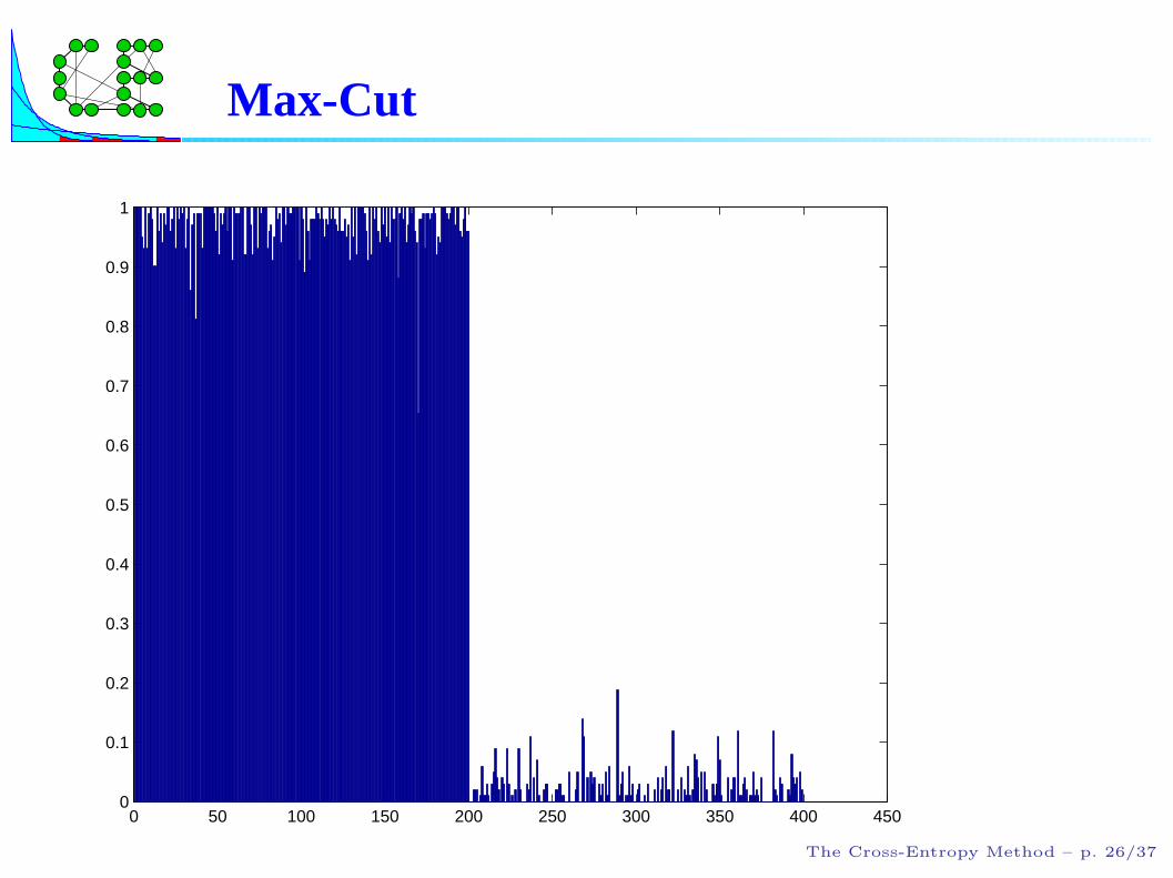
Example: Continuous Optimization

-6 -2 2 60

S(x) = e−(x−2)2 + 0.8 e−(x+2)2

Matlab Program

S = inline(’exp(-(x-2).^2) + 0.8*exp(-(x+2).^2)’);

mu = -10; sigma = 10; rho = 0.1; N = 100; eps = 1E-3;

t=0; % iteration counter

while sigma > eps

t = t+1;

x = mu + sigma*randn(N,1);

SX = S(x); % Compute the performance.

sortSX = sortrows([x SX],2);

mu = mean(sortSX((1-rho)*N:N,1));

sigma = std(sortSX((1-rho)*N:N,1));

fprintf(’%g %6.9f %6.9f %6.9f \n’, t, S(mu),mu, sigma)

Numerical Result

-5 0 50

Iteration 1

-5 0 50

Iteration 4

-5 0 50

Iteration 7

-5 0 50

Iteration 10

Cross-Entropy: Some Theory

Estimate ` := Pu(S(X) ≥ γ) = Eu I{S(X)≥γ} via

I{S(Xi)≥γ}f(X i;u)

g(X i).

The best density (zero variance estimator!) is

g∗(x) :=I{S(x)≥γ}f(x;u)

Problem: g∗ depends on the unknown `.

g(X i).

g∗(x) :=I{S(x)≥γ}f(x;u)

g(X i).

g∗(x) :=I{S(x)≥γ}f(x;u)

g(X i).

g∗(x) :=I{S(x)≥γ}f(x;u)

g(X i).

g∗(x) :=I{S(x)≥γ}f(x;u)

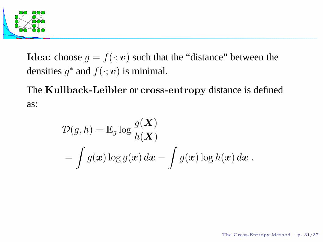
Idea: choose g = f(·;v) such that the “distance” between thedensities g∗ and f(·;v) is minimal.

The Kullback-Leibler or cross-entropy distance is definedas:

D(g, h) = Eg logg(X)

∫g(x) log g(x) dx −

∫g(x) log h(x) dx .

Determine the optimal v∗ from minv D(g∗, f(·;v)) .

This is equivalent to solving

Eu I{S(X)≥γ} log f(X;v) .

Using again IS, we can rewrite this as

Ew I{S(X)≥γ} W (X;u,w) log f(X;v),

for any reference parameter w, where

W (x;u,w) =f(x; .u)

f(x;w)

We may estimate the optimal solution v∗ by solving thefollowing stochastic counterpart:

I{S(Xi)≥γ} W (X i;u,w) log f(X i;v) ,

where X1, . . . ,XN is a random sample from f(·;w).Alternatively, solve:

I{S(Xi)≥γ} W (X i;u,w)∇ log f(X i;v) = 0,

where the gradient is with respect to v.

The solution to the CE program can often be calculatedanalytically.

Note that the CE program is useful only when under w theevent {S(X) ≥ γ} is not too rare, say ≥ 10−5.

Answer: use a multi-level approach.

Introduce a sequence of reference parameters {vt, t ≥ 0} and asequence of levels {γt, t ≥ 1}, and iterate in both γt and vt.

Question: how to choose w so that this is indeed the case?

Toy example 1 (continued)

Recall

f(x;v) = exp

The optimal v follows from the system of equations

I{S(Xi)≥γ} W (X i;u,w)∇ log f(X i;v) = 0.

Since∂

log f(x;v) =xj

we have for the jth equation

I{S(Xi)≥γ} W (X i;u,w)

)= 0 ,

whence,

i=1 I{S(Xi)≥γ}W (X i;u,w)Xij∑N

i=1 I{S(Xi)≥γ}W (X i;u,w),

which leads to the updating formula in step 3 of the Algorithm.

Further research

Multi-extremal constrained continuous optimization.

Noisy optimization.

Simulation with heavy tail distributions.

Incorporating MaxEnt (MinxEnt), e.g. MCE

Multi-actor games

Convergence of CE algorithm.

Further research

Noisy optimization.

Multi-actor games

Further research

Noisy optimization.

Multi-actor games

Further research

Noisy optimization.

Multi-actor games

Further research

Noisy optimization.

Multi-actor games

Further research

Noisy optimization.

Multi-actor games

the cross-entropy method · the cross-entropy method: a uniﬁed approach to combinatorial...

Documents