The curse of dimensionality

Mario KoppenFraunhofer IPK Berlin

Pascalstr. 8-9, 10587 Berlin, GermanyE-Mail: mario.koeppen@ipk.fhg.de

Abstract

In this text, some question related to higher dimensional geometrical spaces will bediscussed. The goal is to give the reader a feeling for geometric distortions related tothe use of such spaces (e.g. as search spaces).

1 Introduction

In one of his essays “Glow, Big Glowworm”[3] Stephen Jay Gould reports on a visitof the Waitomo glowworm caves on Lake Roturura in New Zealand. He witnesseda magnificent natural spectacle, which motivated him for an interesting observation(idem, p. 260):

”‘Here, in utter silence, you glide by boat into a spectacular underground plane-tarium, an amphitheater lit with thousands of green dots — each theilluminated rearend of a fly larva (not a worm at all). (I was dazzled by the effect because I foundit so unlike the heavens. Stars are arrayed in the sky at random with respect to theearth’s position. Hence, we view them as clumped into constellations. This may soundparadoxical, but my statement reflects a proper and unappreciated aspect of randomdistributions. Evenly spaced dots are well ordered for cause. Random arrays alwaysinclude some clumping, just as we will flip several heads in a row quite often so long aswe can make enough tosses — and our sky is not wanting for stars. The glowworms,on the other hand, are spaced more evenly because larvae compete with, and even eat,each other — and construct an exclusive territory. The glowworm grotto is an orderedheaven.)”’

By reading this, the american Nobel laureate Ed Purcell was inspired to perform asmall experiment for the purpose of illustrating theclumpingin random patterns, aboutwhich Gould spoke. The result was presented in thePostscriptumof the essay. Figure1 shows the same experiment in a slightly modified version. Within an image of size256� 256 pixel, 20,000 positions were randomly selected. The difference betweenimage 1 (a) and (b) is as follows: while the positions in figure (a) were selected withuniformly distributedx- andy-coordinates, for figure (b) only positions were allowed,which do not lie within the 8-neighborhood of an already selected position. Hence,figure (a) more ressembles the night sky case, while figure (b) more ressembles the

1

glowworm case, for which each glowworm requires a minimum distance to each of itsneighbors.

(a) (b)

Figure 1: Distribution of 20,000 randomly selected positions in a grid of size256� 256: without any further restrictions (a); and with the restriction that none ofthe selected positions may be direct neighbors (b).

The paradox given by Gould is related to the fact that the observer perceives fea-tures only in figure (a). We consider figure (b) a better representation of randomnessdue to the lack of positional differentiation. There seems to be no region in figure (b)distinguished from any other. But, for figure (a), the human cognition impresses sev-eral distinguishing features, despite of the fact that for the creation of figure (a) therewas never a distinction among positions introduced. This was only the case for figure(b), for the creation of which positions were steadily prohibited!

In a letter to Gould (idem, p. 268), Ed Purcell wrote:

”‘What interests me more in the random field of ’stars’ is the overimposing impres-sion of ’features’ of one sort or another. It is hard to accept the fact that any perceivedfeature — be it string, clump, constellation, corridor, curved chain, lacuna — is a to-tally meaningless accident, having as its only cause the avidity for pattern of my eyeand brain! Yet that is perfectly true in this case.”’

The paradox is related to two interacting factors, a physiological one and a mathemat-ical one.

1. Human physiology of visual perception, based on the model of receptive fields. Itis widely accepted that the receptive fields in the neuronal layers of the visual cortexmay be approximated by GABOR functions. Those functions are characterized by localfrequency and exponential decay. During the so-called preattentive perception, localorientations are determined. Adjacent positions in the “star field” of figure 1 (a) morestrongly guide to the perception of a local orientation than more distant ones. Thefurther steps to the cognition of a local feature shall not be considered here.

2. The second factor is related to a mathematical issue. With the positions itself beingequally distributed, the average distances of these positions are not equally distributedas well. To see this, we present a little numerical experiment. In a square of sidelength1, two points are selected with a uniform distribution, and their distance is computed.This will be repeated for 100,000 times. The so-estimated distances will be dividedamong 100 “cups” according to their magnitudes. The first cup takes distances from0 to

p2=100, the last cup distances from 99=100

p2 to

p2. This gives an estimate

for the probability density of the distribution of the distances of two randomly selectedpoints within the unit square. The computed frequencies, normalized to the total sum1, are given in figure 2. As can be seen, the distances are not equally distributed! Thedistribution is a more left-oriented one. In combination with the exponential decay(see dotted line in figure 2) of receptive fields, we can understand why our perceptionof random patterns is so “clumpsy”: since they are really present, and since they arestrengthened by the functionality of our visual perception.

For now, we will not follow thatunappreciated aspectof random patterns (see [5] formore examples) any further. But we will make a note on the following key aspect: thedistribution of distances of uniformly distributed points in a search space by itself isnot uniformly distributed.

0 0.2 0.4 0.6 0.8 1

0.4

0.8

1.2

1.6

2.0

2.4

2.8

d

p(d)

Figure 2: Estimation of the probability densityp(d) of the distance of two randomlyselected points in the unit square (solid line) and after multiplication with8p

π e�8d2for

simulating the activation of a receptive field (dotted line).

Among the few researchers, which considered such phanomenons in more detail,is Ingo Rechenberg (the “father of evolutionary strategy”). In his book “Evolution-sstrategie’94” [7] there are many examples for such geometrical distortions in the con-text of higher dimensional spaces. Rechenberg even employs those issues for derivinga theoretical model for the progress of an evolutionary strategy, the so-calledspheremodel.

In the following sections, some of those aspects are presented. Section 2 givessome information about highdimensional regular bodies (hypercube, hypersimplex andhypersphere). Section 4 then reconsiders the distribution of distances in highdimen-sional spaces in a more accurate manner.

This will help to give the reader a feeling for what is reliable in higher dimensionalspaces (e.g. search spaces) and what is not, and for which dimensions those effectsbecome to be important.

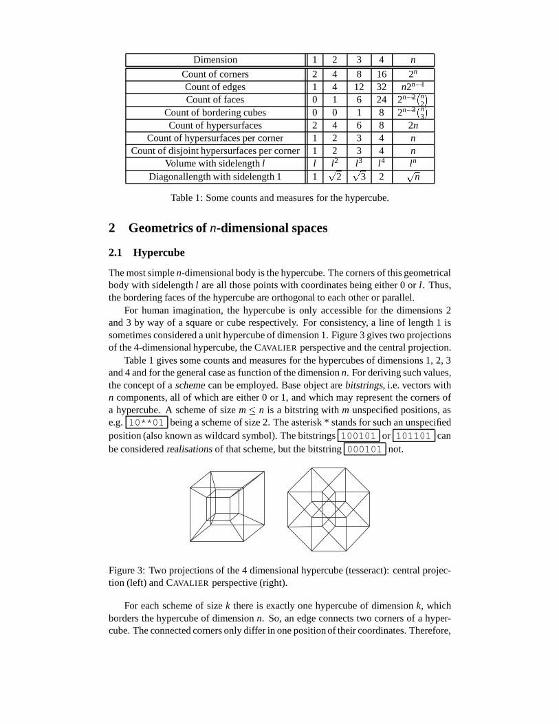
Dimension 1 2 3 4 n

Count of corners 2 4 8 16 2n

Count of edges 1 4 12 32 n2n�1

Count of faces 0 1 6 24 2n�2�n

2

�Count of bordering cubes 0 0 1 8 2n�3

�n3

�Count of hypersurfaces 2 4 6 8 2n

Count of hypersurfaces per corner 1 2 3 4 nCount of disjoint hypersurfaces per corner1 2 3 4 n

Volume with sidelengthl l l2 l3 l4 l n

Diagonallength with sidelength 1 1p

2p

3 2p

n

Table 1: Some counts and measures for the hypercube.

2 Geometrics ofn-dimensional spaces

2.1 Hypercube

The most simplen-dimensional body is the hypercube. The corners of this geometricalbody with sidelengthl are all those points with coordinates being either 0 orl . Thus,the bordering faces of the hypercube are orthogonal to each other or parallel.

For human imagination, the hypercube is only accessible for the dimensions 2and 3 by way of a square or cube respectively. For consistency, a line of length 1 issometimes considered a unit hypercube of dimension 1. Figure 3 gives two projectionsof the 4-dimensional hypercube, the CAVALIER perspective and the central projection.

Table 1 gives some counts and measures for the hypercubes of dimensions 1, 2, 3and 4 and for the general case as function of the dimensionn. For deriving such values,the concept of aschemecan be employed. Base object arebitstrings, i.e. vectors withn components, all of which are either 0 or 1, and which may represent the corners ofa hypercube. A scheme of sizem� n is a bitstring withm unspecified positions, ase.g. 10**01 being a scheme of size 2. The asterisk * stands for such an unspecifiedposition (also known as wildcard symbol). The bitstrings100101 or 101101 canbe consideredrealisationsof that scheme, but the bitstring000101 not.

Figure 3: Two projections of the 4 dimensional hypercube (tesseract): central projec-tion (left) and CAVALIER perspective (right).

For each scheme of sizek there is exactly one hypercube of dimensionk, whichborders the hypercube of dimensionn. So, an edge connects two corners of a hyper-cube. The connected corners only differ in one positionof their coordinates. Therefore,

an edge corresponds to a scheme of size 1. As an example, the scheme00* repre-sents the edge going from corner(0;0;0) to the corner(0;0;1), or the scheme**0the lower face of a cube.

The count of schemes of sizek equals the number of possibilities for selectingkwildcard positions out ofn, multiplied with the number of possibilities to assign 0 or1 to the remainingn� k positions, i.e. 2n�k. Therefrom it follows for the countNn

k ofk-dimensional hypercubes bordering then-dimensional hypercube:

Nnk = 2n�k

�nk

�: (1)

Equation (1) was used to derive the values in table 1. The number of hypersurfaces, towhich a corner belongs, can be found in a similar manner. It has to be counted, howmany schemes of sizen�1 are realized by a given bitstring. This are justn schemes,one for each bit position. The remaining 2n�n = n hypersurfaces of the hypercubeare disjoint to that corner, and each connecting line from the corner to an inner pointof one of those disjoint hypersurfaces completely lies within the hypercube.

All other entries in table 1 are obvious.The volume of an-dimensional unit hypercube is 1. Forn! ∞, the volume of a

hypercube withl > 1 goes to infinity, while forl < 1 it goes to 0. Also, the length ofthe diagonal of a unit hypercube (

pn) goes to infinity, the hypercube becomes more

and more extended. According to [4], the hypercube can be imagined as a highlyanisotropical body, more ressembling a spherical “hedgehog” than a convex body. Theinner ball-like part with radius 1=2 is covered with a large number (2n) of “spikes” oflength

pn=2 (going to infinity for largen) (see figure 4). ”‘The surfaces of cubes are

so horribly jagged that they might even be thought of as being almost fractal.”’ ([4],p. 42).

n-dimensionalunit cube of

volume 1 n-dimensional ballwithin the cube

(radius 1/2)

2n "Spikes" oflength n1/2/2 ≈ ∞

Figure 4: ”‘Spiking Hypercube”’ [4].

Finally, a short computation will show the change of relative volumina within thehypercube, when problem dimension increases. On the main diagonal of a hypercube,a random pointP is selected with coordinatesp1 = p2 = : : : = pn = p and p > 1=2.This way, two subcubes of the hypercube are defined, with one including the point

(0;0; : : : ;0) and a sidelength ofp (A1), and the other including the point(1;1; : : : ;1)and a sidelength of 1� p (A2). Now, P will be shifted slightly by the amountδ. Thequestion is how to chooseδ, given dimensionn, in order to double the ratior of thevolumina ofA1 andA2. The old and new value ofr are given by

rold =

�p

1� p

�n

(2)

rnew =

�p+δ

1� (p+δ)

�n

: (3)

By resolvingrnew=rold = 2 one gets:

δ =p(1� p)

1� p+ np

2| {z }term1

(np

2�1)| {z }term2

: (4)

The interesting property of this result is thatnp

2 with n! ∞ exponentially goes to 1.For largen, term 1 remains nearly constant, while term 2 rapidly goes to 0. This decaydominates term 1 for largen, too.

This means that the necessary shift ofP becomes smaller and smaller, when di-mensionn increases. This decay is even exponential! And, of course, this holds forother ratios as 2 as well. Therefore, mental constructs as the segmentation of a hy-percube into a system of subcubes, standing for classification boundaries or so, arevery instable designs and opted to sudden breakdown when their carriers are slightlymodified.

2.2 Hypersimplex

The hypersimplex is composed ofn+1 equally distanced points in then-dimensionalspace (there are maximaln+1 points inRn with this property). Each two corners of thehypersimplex are connected by an edge of the hypersimplex, each three span a regulartriangle, each four span a regular tetrahedron a.s.f. Then-dimensional hypersimplexis bounded by

�n+1k+1

�hypersimplexes of dimensionk. In that sense, a hypersimplex is

a very compact body.In the appendix, some relations for the hypersimplex are derived. Therefrom, the

volume of a hypersimplex with sidelengtha and dimensionn is given by (see equation(52))

Vn =1n!

rn+1

2n an: (5)

For largen, this expression is dominated by the decay of 1=n!, and the volume goesrapidly to 0 (independently of the size ofa).

For the heighthn of a hypersimplex, i.e. the length of the perpendicular from onecorner to the hypersurface spanned by the remainingn points, one gets (see equation(49))

hn =

rn+12n

a (6)

and for the radiusrn of the surrounding ball, i.e. the hypersphere containing alln+1corner points of the hypersimplex (see equation (50))

rn =

rn

2(n+1)a: (7)

Therefore, for largen, hn andrn are approaching 1=p

2, and it holds

limn!∞

jhn� rnj= 0: (8)

In other words, the center of the hypersimplex gets closer and closer to the centers ofits outer surfaces, the hypersimplex collapses.

The inner angle of the hypersimplex, i.e. the angle between two lines connectingthe center with two corners of the hypersimplex, is (see equation (55))

θ = arccos

��1

n

�: (9)

For largen this goes toπ=2, the hypersimplex becomes a more cube-like body.Of course, all such relations are impossible in finite-dimensional spaces.

2.3 Hypersphere

Finally, then-dimensional hypersphere will be considered. This is the geometricalplace of all those points, which have a distance of maximalR from its center. Also, thesurface of this body, with distance equal toR, is sometimes referred to as hypersphere.The 2-dimensional hypersphere is the common sphere, the 3-dimensional hyperspherethe ball. Sometimes, the unit line is considered a 1-dimensional hypersphere.

For obtaining the volume of a hypersphere of radiusR, it has to be distinguishedwhethern is odd or even. Forn= 2p even one gets (see appendix)

V2p =R2pπp

p!(10)

and forn= 2p+1 being odd

V2p+1 =R2p+12p+1πp

1�3�5� : : : � (2p+1): (11)

With the following definition forp!!

p!! = 1 for p< 2 (12)

p!! = p� (p�2)!! else (13)

this can be given in a more compact manner

Vn =2[(n+1)=2]π[n=2]

n!!Rn (14)

with [x] the largest integer smaller or equal tox.

n Vn

1 2.000002 3.141593 4.188794 4.934805 5.263796 5.167717 4.724778 4.058719 3.2985110 2.55016

Table 2: Volume of the unit cube for the dimensions 1 to 10.

2 4 6 8 10 12 14

0.2

0.4

0.6

0.8

1

n

Sn/Cn

1

Sn

Cn

Figure 5: Ratio of the volumes of unit hypersphere and embedding hypercube of side-length 2 up to the dimension 14.

As it was the case for the hypersimplex, the volume of a hypersphere goes to 0,independent from the size of its radius. Table 2 gives the volumes of some unit cubesfor n= 1; : : : ;10. The hypersphere forn= 5 has the biggest volume, but this dependson R. Especially, forR= 1=

p2, the hypersphere attains its maximum in “our” 3-

dimensional world.

As an example consequence for search spaces, the ratio of volumes of unit hy-persphere and embedding hypercube (with a sidelength of 2) will be considered (seefigure 5). Despite of the fact that the volume of the hypercube goes to infinity, and thehypersphere touches all faces of the hypercube (i.e. at 2npoints), the volume of the em-bedded hypersphere goes to 0! Moreover, forn> 10 we could neglect this volume partwithin the hypercube for all practical computations. This is an important distinctionbetween search methods, which explores the hypercube, and search methods, whichexplores the hypersphere. The last ones will not “see” very much from their world.

Also, it has to be noted that the term “high dimension” may refer to values ofn assmall as 10 or so.

3 Short Break: The fourth spatial dimension

Geometrical relations in spaces with more than three spatial dimensions seems to beimpossible to imagine. This is a remarkable property of the human cognition, thediscussion of which will be shortly given in this section.

We will concentrate on the most simple question in this context about a fourthspatial dimension. No mathematical training seems to be suitable to access a mentalstate, which makes it possible to operate with the tesseract in the same way we are usedto operate with objects in the 2- or 3-dimensional space. Therefore, it is no wonderthat most efforts in this direction were made a little bit apart from traditional science.

Nevertheless, the choices offered by a possible access to a fourth spatial dimensionare astonishing. Just to name a few:

� It would be possible to directly perceive the interior of a body.

� The content of a box could be taken without opening the box.

� A node could be removed from a string without moving the ends of the string.

� A body could be lifted without external forces.

� A body could be moved into its mirror form.

Of course, this reminds one more on the tricks of a magician than on real effects ofphysical interactions. So, first efforts on speculating about a fourth dimension can befound in some esoteric circles of the 19th century. The fourth dimension was regardedas the world of demons and ghosts, but even as the world where god and his angelsused to live as well. One of the first more serious discussions of a fourth spatial di-mension can be found in the essay “Flatland” of Edwin Abbott Abbott (1838–1926)from 1884 [1]. Besides of being a mathematical excurse into the questions of livingin a 2-dimensional world, the essay also offers some critque on the victorian society.The main character of this essay, A Square, is sentenced to prison for teaching his“flat-minded” contemporaries the existence of a 3-dimensional world.

Another person of interest is Charles Howard Hinton (1853–1907), who used tolive, in modern words, a wild life. He developped a system for memorizing an arrange-ment of 36�36�36= 46656 cubes, each of which carrying a unique latin name. So,he created something like a “threedimensional retina” and became able, after yearsof training, for mental images of spatial arrangements even in a 4-dimensional space.Also Henri Poincar´e reports on such a successfull training in his book “Last Essays”[6]. In a more pessimistic mood we find Rudy Rucker ([8], p. 7): “It is very hard tovisualize such a dimension directly. Off and on for some fifteen years, I have tried todo so. In all this time I’ve enjoyed a grand total of perhaps fifteen minutes’ worth ofdirect vision into four-dimensional space.”

Interesting enough, Poincar´e also considered the question about the three dimen-sional nature of our world, and he gives a surprisingly modern-sounding idea. Accord-ing to him, a thinking entity, as the human beings are, could assign to their world ei-ther dimension they like, since all of them are mathematically equivalent. Thereby, theworld appears to be an abstract premise for sensoric perception and muscular activity,and spatial dimensions are basically a mental product. The choice for three depends

on the configuration of the human nervous system and the so-acquired evolutionaryadvantage. By using two 2-dimensional retinas, the movement of the two hands hasto be monitored. A dimension of 2 would not suffice to perform such a control, and adimension of 4 would allow for movements, during which the hands may even shortlybe disconnected from the remaining body. So, a dimension of 3 seems to be a goodcompromise.

Basing on such arguments, mental operations with more than three dimensionsseems to be possible, but dangerous for the being undergoing such experiments in our3-dimensionalorganizedworld as well.

The question should not mistaken with the question for a physical fourth dimen-sion. The limitation of feeling unable to imagine a tesseract is related to human cogni-tion, and it hints on an evolutionary designed human being without any need for suchabilities. Concepts of modern physics, as quantum theory, spin, quarks, black holes orstring theory rely on abstractions beyond human cognition as well, and lead to manycontradictions for our thinking, but this is related to the use of models to describeobjective matter.

So, considering time as a fourth dimension is not the same as considering a fourthspatialdimension. While it is a good trick for describing relativity, it is not just more:we can not move forth and back in time. Also string theory, which offers even tendimensions, six of which got lost after creation of the universe, has similar disadvan-tages.

Therefrom, this short consideration of a fourth spatial dimension should show thatwe could learn something about the “bootstrapping” of human cognition, or, in otherwords, the way that thinking is rooted into its material base, the central nervous system.

Whether there are any physical principles, which may temporarily cross a fourthdimension, remains an open question. Up to now, there is no experiment known whichdemonstrates the fact of a merely 3-dimensional world, and also there is no fact knownfor which a 3-dimensional world would be optimal. On the other hand, the practicalpossibilities offered by such anaccess would be astonishing.

Last, but not least, the question for a fourth dimension has inspired arts as well. In[2] there are lots of computer generated pictures on this subject. The 1954 SalvadorDalı painting “Corpus Hypercubicus” shows the famous religious motive using an un-folded tesseract. The Cubists also tried in their multi-perspective approach to capturethe idea of a choice for simultaneous perception of different aspects of the same thing- as it would be a simple act for a fourdimensional (thinking) being, knowing aboutCharles Hintons’Kataperspective.

4 Equal distribution in the hypercube

4.1 Square

As it was discussed at the beginning of this text, equally distributed points in a squarewill not necessarily give equally distributed distances (pairwise distances or distanceto one corner of the square). In the following, this will be derived mathematically.

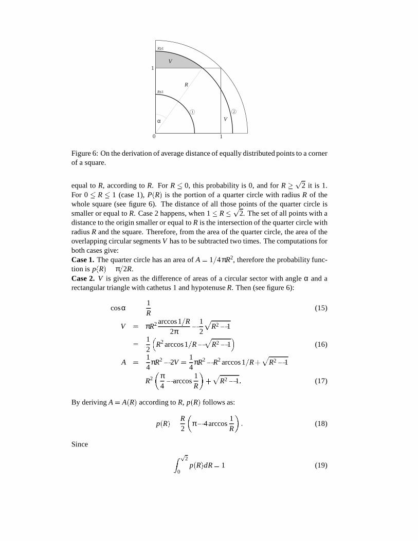
For doing so, the probability densityp(R) of the distancesRof equally dsitributedrandom points will be determined. This is given by the derivation of the probabilityfunctionP(R), which describes the probability of obtaining a distance value lower or

α

R

V

1 2

R≤1

R≥1

1

1

V

0

Figure 6: On the derivation of average distance of equally distributed points to a cornerof a square.

equal toR, according toR. For R� 0, this probability is 0, and forR� p2 it is 1.For 0� R� 1 (case 1),P(R) is the portion of a quarter circle with radiusR of thewhole square (see figure 6). The distance of all those points of the quarter circle issmaller or equal toR. Case 2 happens, when 1� R� p2. The set of all points with adistance to the origin smaller or equal toR is the intersection of the quarter circle withradiusR and the square. Therefore, from the area of the quarter circle, the area of theoverlapping circular segmentsV has to be subtracted two times. The computations forboth cases give:Case 1.The quarter circle has an area ofA= 1=4πR2, therefore the probability func-tion is p(R) = π=2R.Case 2.V is given as the difference of areas of a circular sector with angleα and arectangular triangle with cathetus 1 and hypotenuseR. Then (see figure 6):

cosα =1R

(15)

V = πR2 arccos1=R2π

� 12

pR2�1

=12

�R2 arccos1=R�

pR2�1

�(16)

A =14

πR2�2V =14

πR2�R2 arccos 1=R+p

R2�1

= R2�

π4�arccos

1R

�+p

R2�1: (17)

By derivingA= A(R) according toR, p(R) follows as:

p(R) =R2

�π�4arccos

1R

�: (18)

Since

Z p2

0p(R)dR= 1 (19)

1

0.2

0.4

0.6

0.8

1

20R

P(R)

1 2

(a)1

0.25

0.5

0.75

1

1.25

0 2R

p(R)π/2

1 2

(b)

Figure 7: Probability function (a) and probabilitydensity (b) of the distances of equallydistributed points to a corner within the unit square.

1 2 3 4 5 6 7 8 9 100.543 0.543 0.544 0.541 0.541 0.541 0.540 0.542 0.540 0.539

Table 3: Ten experimentally computed values for the average distance of 20,000 ran-dom points from a corner.

there is no need to normalizep(R).Figure 7(a) and (b) shows the plots ofP(R) andp(R). As can be seen, there is no

uniform distribution of the distances (which would be given by a flat line). To get theexpectation value of the distance, the first moment has to be computed:

Z p2

0xp(x)dx=

p2+ ln(

p2+1)

3' 0:7652: (20)

So we get for the expectation value of the distance of a randomly selected point withina square with diagonallength 1 to one corner

E[R=p

2]' 0:541: (21)

Table 3 gives some experimentally computed values, using 20,000 random points ineach case.

For the variancy one gets:

σ2[R=p

2] =12

Z p2

0(x�E[R])2p(x)dx

=4�2

p2 log(1+

p2)� log(1+

p2)

2

18' 0:0405 (22)

Table 4 gives ten experimentally computed values, using 10,000 random points in eachcase.

To summarize: equally distributed points in a unit square will have an averagedistance of 0:76�0:28 to a corner of the square (with 0.28 given asσ[R]).

1 2 3 4 5 6 7 8 9 1040.5 40.5 39.9 39.9 40.5 40.7 40.8 39.5 39.9 41.6

Table 4: Ten experimentally computed values for the variancy of 10,000 randompoints, multiplied with 1000.

R� 1 1� R�p2p

2� R� p3

Figure 8: Three cases for the intersection of eighth ball and unit cube.

4.2 Cube

Now, the computations will be given for the case of a unit cube. As can be seen fromfigure 8, this time there are three cases to consider.Case 1: 0� R� 1. The eighth ball lies completely within the cube, therefore

P(R) =16

πR3: (23)

Case 2: 1� R� p2. Here, the eighth ball sticks out of the cube on its three faces.Each of these quarter ball caps has the heightR�1. The volume of a ball capκ withradiusR and heighth isVκ = 1=3πh2(3R�h). Therefore

P(R) =16

πR3� 34� 13

π(R�1)2(3R�R+1)

=16

πR3� 14

π(R�1)2(2R+1): (24)

Case 3:p

2� R� p3. The quarter ball caps start to overlap. The resulting body (acube corner sticking out of the eighth ball) is hard to describe mathematically. Becauseonly a small part of the functionsp(R) andP(R) is covered by this case, instead of anexact computation a spline interpolation was used.

The details of the derivation ofP(R) will be omitted here. Figure 9 gives the plotsof both functions. The skewness of the distribution, compared with the square case,has increased.

From the first moment the expectation valueE[R=p

3] and the variancyσ2[E=p

3]can be computed. It follows for the average distance in a cube of diagonallength 1 thevalue 0.55 and for the variancy 0.026. In the unit cube, equally distributed randompoints will have an average distance of 0:96�0:28 to each corner.

4.3 General case

For the general casen> 3, the formal computations become too complex. Thats whywe restrict our attention on some numerical experiments.

1

0.2

0.4

0.6

0.8

1

2 30

P(R)

R

1 2 3

(a)1

0.25

0.5

0.75

1

1.25

1.5

2 30

1 2 3

R

p(R)

(b)

Figure 9: Probability function (a) and density (b) for the distances of random pointswithin the unit cube to a corner.

20 40 60 80 1000.4

0.45

0.5

0.55

0.6

0.65

En[R]

n

(a)20 40 60 80 100

0

0.01

0.02

0.03

0.04

0.05

σn(R)

n

(b)

Figure 10: Expectation value and variancy of the distance of a random point of ahypercube with diagonallength 1 to one of its corners.

The simulation is quite simple: for given dimensionn, n equally distributed ran-dom numbersxi from [0;1] are generated. Then, compute

Rn =1pn

qx2

1+x22+ : : :+x2

n: (25)

This is repeated for a given number of trials, and the expectation value and variancyof the valuesRn is computed. To get the plot in figure 10 (a), forn going from 1 to100, in each case 2000 trials were made, for figure 10(b) 1000 trials. Two things areobvious: the expectation values approaches a constant value (R∞ of about 0.58); andthe variancy decays to 0 with the order of about 1=

pn.

On a first glance, this may be a surprise. For higher dimensions, the reliabilityof the fact that a random point will have a fixed distance to a corner of a hypercube,rapidly goes to 1. The probability of obtaining a different distance becomes nearly 0.Therefore, it is impossible to stay nearby the corner region of a cube.

It has to be noted that the points itself remain random. They are still uniformlyscattered over the whole volume of the hypercube. The convergence is only a statisticalone. This can be understood in the sense that the majority of the hypercube volume isconcentrated in the inner part, and the portion of the spikes (corner regions) goes downto 0.

Figure 11 illustrates this fact. By numerical simulation, the probability densityfunctions for dimensions 2, 3, 4, 5 , 10, 30, 50 and 100 have been obtained. Withincreasing dimension one gets a more and more bell shaped curve.

1.5

3.0

4.5

6.0

7.5

9.0

n=2n=3

n=4

n=5

n=10

n=30

n=50

n=100

20 % 40 % 60 % 80 % 100 %

N

Figure 11: Probability density functions for the distance of a random point from thecorner of a unit hypercube for dimensions up to 100.

What is the exact value ofR∞? For getting this value, equation (25) is re-consideredunder the viewpoint thatR2

n is the expectation value ofn squares of equally distributedrandom numbers from[0;1] as well. Now,n is considered to be infinitesimal large, butall those random numbers are “rounded” up to the nearest out of a set ofm equally-distanced values from[0;1]. So,R∞ will be derived as a function ofmwith mgoing toinfinity. To illustrate this, we consider the casem= 3 with the three values 0, 1=2 and1. So, 0.321 will be rounded to 0.5, 0.872 to 1 and 0.123 to 0. There are three cases:

1. Random numbers from 0 to 0.25 will be rounded to 0. This happens in 1=4 ofall cases. The square will take the value 0 in 25% of all trials.

2. Random numbers from 0.25 to 0.75 will be rounded to 0.5. Hence, with a prob-ability of 1=2 the square will have the value 0.25.

3. Random numbers from 0.75 to 1 will be rounded to 1. This happens with prob-ability 1=4, and the square will have the value 1.

Thus follows for the expectation value of the square after rounding:

R∞(3) =14�0+ 1

2� 14+

14�1=

38: (26)

0 1/m2 4/m2 9/m2 (m-1/m)2 1

0 1/m 2/m 3/m (m-1)/m 1

Figure 12: Computing the expectation value of the square of random numbers from[0;1] by rounding them tom intervall values.

Now we consider the general case of(m+1) equally distanced intervall values forrounding (see figure 12). The intervall values are 0;1=m;2=m;3=m; : : : ;(m�1)=m;1.There are(m� 1) intervalls of length 1=m, for which the squares take the values1=m2;2=m2; : : : ;(m�1)2=m2, and two intervalls of length 1=2m, with the square being

0 and 1. ForR∞(m), we obtain:

R∞(m) =1m

�1

m2 +4

m2 +9

m2 + : : :+(m�1)2

m2

�+

12m

=1

m3

�12+22+32+ : : :+(m�1)2�+ 1

2m

=1

m3

(m�1)m(2m�1)6

+1

2m

=13+

16m2 : (27)

In this derivation, the formula for the sum of the firstk square numbers∑ki=1 i2 =

1=6�k(k+1)(2k+1) was used. For the limes we get:

R2∞ = lim

m!∞R∞(m) =

13: (28)

Hence, the expectation value goes to 1=p

3' 0:57735, which is quite similar to theestimate of figure 10.

The presented approach is not suitable for getting the decay of variancy as well.But, if the magnituden of the dimension is considered to be a measure for the exactnessof the computation ofR∞, from equation (28) it can be seen that variancy goes downwith the order of about 1=

pn.

Finally we will mention the question for thepairwisedistance of two randomlyselected points:

D2∞ = lim

n!∞En[(xi�xj )

2]: (29)

This can be derived in a manner similar to the derivation ofR∞. One gets for theexpectation value of the product of two randomly selected points from[0;1] the value1=4. For the average distance it follows:

D2∞ = 2E[x2

i ]�2E[xixj ] =23�2� 1

4=

16: (30)

thusD∞ = 1=p

6 ' 0:40825. In higher dimensions, we will not meet the “Gould-Effect” (see p. 2), since the pairwise distances of random points approach a constantvalue. This may give raise to the question whether pattern recognition is even possiblefor beings using a higherdimensional sensation space. We see more evidence for thefact that with increasing dimension probabilities become reliabilities.

5 Summary

Some geometrical and statistical issues of higherdimensional spaces, i.e. spaces with adimension greater than 3, have been discussed. Despite of the fact that they are simplyaccessible from a formal point of view, their geometrical and statistical properties maygive some problems. This is only partially related to the limitation of human cognitionto perform mental operations on such objects as the 4-dimensional hypercube. Themore important are geometric distortions of positional and volume relations, whichfinally repress randomness at all. In particular, evidence was given for the followingclaims:

� The ratio of the volume of a hypersphere to the volume of its embedding hyper-cube goes to 0 by the order ofn!. This means for search methods that it makes abig difference, whether searchspace is explored spherically or “blockwise.”

� Segmentations become unstable according to relative ratios of volumes. Byslightly shifting one of the segmentation boundaries and for sufficient largen,the ratios of volumina could be changed to either value.

� The distance of a randomly selected point in a hypercube of diagonallength 1 toone corner gets closer and closer to 1=

p3, asn increases. Hence, for random

search it is impossible to select positions nearby the corner of a hypercube.

� Two randomly selected points in a hypercube will have nearly the same distancefor largern. Therefrom,(n+1) of them will give a hypersimplex, the volumeof which rapidly goes to 0. An estimation of the volume occupied by a randomset of points (basing e.g. the Monte Carlo method) is no more reliable.

� Features in random patterns (e.g. textures) are a unique property of lowdimen-sional spaces.

Therefore, using analogies from 2- or 3-dimensional spaces for higherdimensionalspaces always has to be done with care.

A Hypersimplex and Hypersphere

A.1 The generalized Cavalier principle

A cone over an object (base) to a pointA not belonging to this object is defined as theset of all lines connectingA with any of the interior points of the object. The distanceof A from the object is defined as the height of the cone. The CAVALIER principle saysthat two cones have the same volume if their bases and heights are equal.

Figure 13: Splitting of a cube into three coni with equal volume. A cornerV of thecube is connected to all points of a face, which does not touch the corner point.

Now consider the coni, which are generated by connecting a corner of a cube withall points of a face, which is disjoint with the corner (there are three such faces). Thus,

the cube is splitted into three disjoint coni, which have the same volumesaccordingto the CAVALIER principle (in all cases, base is a face of the cube, and height is thesidelength of the cube). Since a cube with sidelengthR has a volume ofR3, each ofthe subconi has a volume ofR3=3. With A = R2 being the area of the base of such aconus, andh= Rbeing its height, this can be written asVconus= hA=3 as well.

When the base of a conus is not a square, the base is assumed to be covered by asequence of smaller squares, which approximate the area of the base. For each conusover a subsquare, the equation for the volume holds, and in the limiting case, for thevolume of a conus with baseA and heighth one gets:

V =13

h�A: (31)

Note that for the validity of equation (31) the base needs not to be flat.A similar relation can be given for then-dimensional case as well. Then, the

hypercube is split inton disjoint coni, for a corner of a hypercube being disjoint toexactlyn hyperfaces (see p. 5). Therefore, an-cone with baseA and heighth has a(hyper)volume of

V =1n

h�A: (32)

A.2 Volume of a hypersphere

The volume of a hypersphere could be derived by using multiple integration, but thereis a more simple way1.

A n-ball is the set of all points inn-dimensional space, which have the maximumdistance ofR from a given central point, i.e. an-dimensional hypersphere. A(n�1)-sphere is the set of all points with its distance to the center being exactlyR, i.e. thesurface of then-ball.

A n-ball is the cone over its surface as well. This cone has the base ofAn�1(R) andthe heightR. Thus, due to the generalized CAVALIER principle, for volumeVn(R) of an-ball and its surface volumeAn�1(R), the following relation holds:

Vn(R) =1n

R�An�1(R): (33)

Also An(R) can be given as a function ofVn�1(R). For doing so, consider the embed-ding of the ball into a tophat with the same radius.

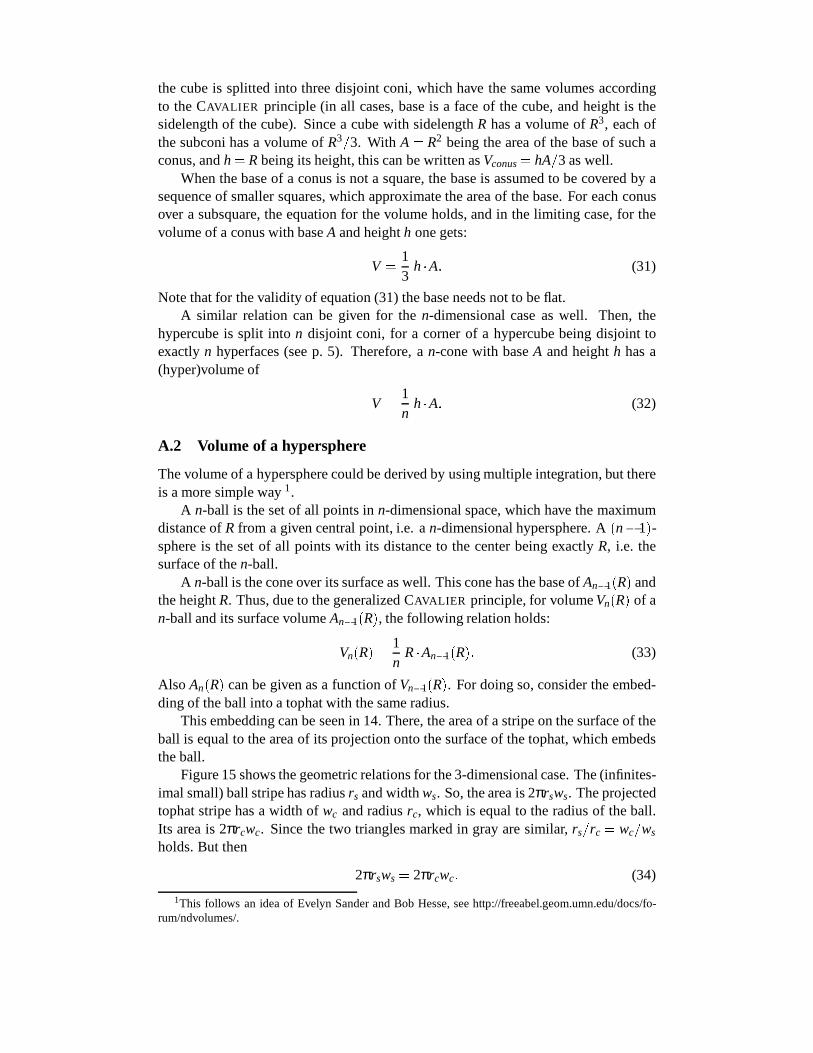
This embedding can be seen in 14. There, the area of a stripe on the surface of theball is equal to the area of its projection onto the surface of the tophat, which embedsthe ball.

Figure 15 shows the geometric relations for the 3-dimensional case. The (infinites-imal small) ball stripe has radiusrs and widthws. So, the area is 2πrsws. The projectedtophat stripe has a width ofwc and radiusrc, which is equal to the radius of the ball.Its area is 2πrcwc. Since the two triangles marked in gray are similar,rs=rc = wc=ws

holds. But then

2πrsws = 2πrcwc: (34)

1This follows an idea of Evelyn Sander and Bob Hesse, see http://freeabel.geom.umn.edu/docs/fo-rum/ndvolumes/.

Figure 14: A stripe on the surface of the ball has the same area as its projection ontothe surface of a tophat, which embeds the ball.

.

rs

rc

ws wc

M

Figure 15: Similar triangles for the proof that ball and tophat stripes do have the samearea. It isrs=rc = wc=ws.

This is also true in the general case. The(n�1)-sphere has the same volume as thecrossproduct of circle and(n�2)-ball.

An�1(R) = 2πR�Vn�2(R) (35)

Together with equation (33) this gives a recursive formula forVn(R):

Vn(R) =2πn

R2Vn�2(R): (36)

Using

V1(R) = 2R (37)

V2(R) = πR2 (38)

one gets for even and odd values ofn:

V2p(R) =πp �R2p

p!(39)

V2p+1(R) =2p+1 �πp �R2p+1

1�3� : : : � (2p+1)(40)

A.3 Hypersimplex

For obtaining the volumeVn of a n-dimensional hypersimplex, the generalized CAV-ALIER principle can be applied directly. Figure 16, which shows the 3-dimensionalcase, should stand for the general case. The(n+1)th cornerA of a n-dimensional hy-persimplex with borderlengtha is placed at the heighthn above the base hypersimplex,which is composed of the remainingn points. Therefore, the volume is

Vn =1n

hnVn�1: (41)

SinceV1 = a is known, one basically has to get a formula forhn in order to obtain anexpression forVn. Two relations will be used, which can be verified by using the twotriangles41 and42 in figure 16. Bern the radius of the hypersphere surroundingthe hypersimplex. Triangle41 =4AMN is generated from the following three points:cornerA; the perpendicularM from A onto the base hypersimplex (of dimension(n�1)); and the centerN of a hypersimplex of dimension(n�2), which is disjoint toA(in the figure the lineBD). Triangle42 =4AMB is composed from the sameA andMand a further cornerB, which also borders the hypersimplex containingN.

A

NM

B

ahn-1

hn

rn-1

hn-1-rn-1 C

D

2 1

Figure 16: Derivations for a hypersimplex.

From41 one gets

41 : h2n+ r2

n�1 = a2 (42)

and from42 respectively

42 : h2n�1 = hn2 +(hn�1� rn�1)

2: (43)

This can be combined:

a2� r2n�1 = h2

n�1� (hn�1� rn�1)2 (44)

a2 = 2hn�1rn�1 (45)

and therefore, by replacingn�1 byn:

a2 = 2hnrn: (46)

This means: ifhn�1 andrn�1 are known,hn andrn can be computed by

h2n = a2� r2

n�1 (47)

rn =a2

2hn: (48)

For the regular triangle the values ofh2 and r2 are known. It ish2 =p

3=2a andr2 = a=

p3. So, the values ofhn andrn can be determined recursively.

hn =

rn+12n

a (49)

rn =

rn

2(n+1)a: (50)

For the volume of the hypersimplex follows:

Vn =1n

rn+12n

aVn�1 (51)

which gives

Vn =1n!

rn+1

2n an: (52)

For n= 1 this holds byV1 = a. Be equation (52) true forn= k. Then, forn= k+1 itfollows:

Vk+1 =1

(k+1)!

rk+22k+1 ak+1 =

1k+1

�s

k+22(k+1)

a� 1k!

rk+12k ak

=1

k+1hk+1Vk (53)

and the equation holds forn= k+1 as well. This verifies equation (52).For the inner angleθ of a triangle with the sidesrn, rn anda and by using the cosinetheorem one gets

a2 = 2r2n(1�cosθ); (54)

and, if using equation (50)

θ = arccos

��1

n

�: (55)

References

[1] E. A. ABBOTT, Flatland, Penguin Books, 1987.

[2] T. F. BANCHOFF, Beyond the Third Dimension, Scientific American Library,1996.

[3] S. J. GOULD, Bully for Brontosaurus, Penguin Books, 1991.

[4] R. HECHT-NIELSEN, Neurocomputing, Addison–Wesley Publishing Company,Reading, MA, u.a., 1991.

[5] D. MARR, Vision, MIT Press, 1981.

[6] H. POINCARE, Mathematics and Science: Last Essays, Dover Publications, Inc.,New York, 1963.

[7] I. RECHENBERG, Evolutionsstrategie’94, frommann–holzboog, 1994.

[8] R. RUCKER, The Fourth Dimension, Houghton Mifflin Company, Boston, 1984.