The delayed and noisy nervous system: implications for neural control

This article has been downloaded from IOPscience. Please scroll down to see the full text article.

2011 J. Neural Eng. 8 065005

(http://iopscience.iop.org/1741-2552/8/6/065005)

Download details:

IP Address: 134.173.140.165

The article was downloaded on 17/10/2012 at 15:52

Please note that terms and conditions apply.

View the table of contents for this issue, or go to the journal homepage for more

Home Search Collections Journals About Contact us My IOPscience

IOP PUBLISHING JOURNAL OF NEURAL ENGINEERING

J. Neural Eng. 8 (2011) 065005 (11pp) doi:10.1088/1741-2560/8/6/065005

The delayed and noisy nervous system:implications for neural controlJohn G Milton

Joint Science Department, W. M. Keck Science Center, 925 N. Mills, Claremont, CA 91711, USA

E-mail: jmilton@jsd.claremont.edu

Received 7 February 2011Accepted for publication 16 June 2011Published 4 November 2011Online at stacks.iop.org/JNE/8/065005

AbstractRecent advances in the study of delay differential equations draw attention to the potentialbenefits of the interplay between random perturbations (‘noise’) and delay in neural control.The phenomena include transient stabilizations of unstable steady states by noise, control offast movements using time-delayed feedback and the occurrence of long-lived delay-inducedtransients. In particular, this research suggests that the interplay between noise and delaynecessitates the use of intermittent, discontinuous control strategies in which correctivemovements are made only when controlled variables cross certain thresholds. A potentialbenefit of such strategies is that they may be optimal for minimizing energy expendituresassociated with control. In this paper, the concepts are made accessible by introducing themthrough simple illustrative examples that can be readily reproduced using software packages,such as XPPAUT.

1. Introduction

The performance of motor tasks is enhanced by the presence oftime-delayed sensory feedback [1, 2]. However, a fundamentaland unresolved issue in neural motor control concerns the roleplayed by time delays. These time delays arise because axonalconduction velocities and distances between neurons arefinite. As a consequence of conduction and neural integrationtime delays, reaction times are surprisingly long (100s ofmilliseconds [3]) and furthermore increase as the complexityof the voluntary task increases [4]. Should the effects oftime delays be ignored? Does their presence necessitate theexistence of compensatory mechanisms to lessen their effects[5, 6]? Or has the nervous system learned through evolution totake advantage of time delays in some, as yet to be discovered,manner?

The neuroscience of motor control has a long traditionof borrowing concepts from engineering [7]. From thisperspective, time delays present obstacles for the orderlycontrol of voluntary movements. For example, long timedelays are potentially destabilizing and represent a barrierfor the control of movement on time scales shorter than thedelay. In turn it is argued that these obstacles necessitatethe requirement for anticipatory mechanisms that lessenthe effects of delays [5, 6], such as delay compensatory

mechanisms based on forward models [8] and predictivemechanisms based on the concept of an internal inverse model[9], or combinations thereof [10–12]. However, since thesemechanisms are themselves implemented by populations ofneurons, they must ultimately be understood in the contextof delay differential equations (DDEs). Thus, the importanceof an understanding of the effects of time delays on neuraldynamics cannot be easily dismissed. In defense of delays,it is well known that the upright position of an invertedpendulum, an unstable fixed point, can be stabilized usingtime-delayed feedback [14–17]. Moreover, the roles playedby stable, non-stationary behaviors that frequently arise inthe presence of delay when steady states become unstableon motor control have received little attention. Indeed, it isincreasingly recognized that nonlinear dynamic phenomena,such as synchronization of oscillators [13, 18], multistability[19] and critical phenomena [20], are important aspects ofneurodynamics. Even anticipatory control is possible usingtime-delayed feedback [21–23].

The ability of a control strategy to stabilize an invertedpendulum is a widely used benchmark [24]: the better theperformance, the more robust the control strategy. Recentexperiments on human balancing of an inverted pendulum[25–27] suggest that noise and delay may actually havebeneficial effects for neural control. Specifically, it has

1741-2560/11/065005+11$33.00 1 © 2011 IOP Publishing Ltd Printed in the UK

J. Neural Eng. 8 (2011) 065005 J G Milton

been argued that the interplay between noise and delaynecessitates an intermittent control strategy in which activecorrective movements are made only when necessary. Suchstrategies suggest that the nervous system ultimately choosesmotor control strategies that minimize its energy expenditures[28, 29].

Here I review the effects of the interplay between noiseand delay on feedback control. An effort is made to present thematerial within a conceptual framework accessible to readerswith minimal mathematical background through the use ofexamples that can be easily studied with a computer softwarepackage such as XPPAUT [30]. In section 2, a simple exampleof delayed feedback is used to illustrate the effects of delay,feedback gain and memory, and in section 3 the effects of noiseare introduced. Section 4 draws attention to two scenarios thatenable delay feedback mechanisms to provide ‘fast control’,and section 5 discusses transient behaviors unique to systemswith delay.

2. Background

Mathematical models of neural feedback control take the formof DDEs. An example is the first-order DDE

x(t) = f (x(t), x(t − τ)), (1)

where τ is the time delay, f is the feedback and x(t), x(t − τ)

are, respectively, the values of the state variables at timest, t − τ [14, 31–33]. The notation x denotes dx/dt . In orderto specify a unique solution to (1), it is necessary to specifyan initial function φ(s), s ∈ [t0 − τ, t0] ≡ �. Over the last10–15 years, there has been growing interest in the effects oftime delays on neural control: control with two discrete timedelays [34] or a distribution of time delays [35], multistability[37–39] and chaos [40–42] and considerations of the dynamicsof pulse-coupled neural networks [43, 44]. Moreover, it isquite likely that feedback includes the effects of terms relatedto x(t − τ) and x(t − τ) [36], and possibly even higher-order derivatives [45]. Although contributions to feedbackrelated to x can be estimated by peripheral mechanoreceptors,contributions related to x and higher-order derivatives likelyrequire cortical processing [16]. Here we confine our attentionto (1) in order to examine the effects of interplay between noiseand the choice of � on control.

For a given choice of f , the dynamics of (1) depend on τ ,feedback loop gain and �. In order to appreciate the relativeroles played by these factors, it is useful to consider the specificexample

x(t) = αx(t − τ), (2)

where α is a constant and x(t) and x(t − τ) are, respectively,the values of the state variable at times t and t − τ . Thisequation is sometimes referred to as the Wright equation[33, 46, 47]. The advantage of considering this equation isthat a number of important concepts for the discussion thatfollows can be introduced using familiar techniques.

When τ = 0, we have

x(t) = αx(t). (3)

The fixed point, determined by setting x(t) = 0, is x∗ = 0.Making the usual Ansatz that solutions are of the form eλt ,where λ is an eigenvalue, we obtain the characteristic equation

λ = α.

Hence, the condition for stability of the fixed point x∗ is α < 0.In order to uniquely determine a solution of (3), it is necessaryto specify an initial condition x(t0).

We can follow the same approach to investigate thebehavior of (2) when τ > 0, obtaining the characteristicequation

λ = α e−λτ , (4)

which is a transcendental equation. Suppose that λ = γ + ifis a complex eigenvalue. Then using Euler’s relationship, wecan write e−λτ = e−γ [cos f τ − i sin f τ ], and hence we seethat (4) will have an infinite number of solutions. This meansthat we cannot specify a unique solution using an initial value;we need to specify an initial function, �. Typically in softwarepackages, such as XPPAUT, � is defined in two parts: a valueat t0, x(t0), together with the function φ′(s), s ∈ [t0 − τ, to)

(see, for example, the appendix in [48]). This representationfacilitates comparison with the case when τ = 0.

There are two real negative roots for 0 < α < 1/τe.At α = 1/τe, these roots merge to form a complex pair ofeigenvalues with a negative real part. The real part of theeigenvalue pair is the first to become positive as τ increases.The condition for instability can be obtained by assuming thatγ = 0. Using Euler’s relationship, we can rewrite (4) as

if

α= −[cos f τ − i sin f τ ],

which can be solved by equating real and imaginary parts. Thecritical frequency, fc, and critical delay, τc, for which instabilityoccurs are, respectively, α and π/2α. Figure 1(a) shows thebehavior of (2) for different choices of τ . For 0 < τ < 1/αe,the solutions of (2) decay monotonically, damped oscillationsexist when 1/αe < τ < π/2α and diverging oscillations occurwhen τ > π/2α.

What is the contribution of the remaining infinite numberof complex conjugate pairs of eigenvalues to the behaviorof (2)? The complex conjugate pairs of eigenvalues can beobtained by rewriting (4) as [49],

s = ces ,

where s = −λτ and c = −ατ . One solution s = u + iv existson each strip,

2pπ < v < (2p + 1)π, p = 0, 1, 2, . . . ,

at the intersection of the appropriate branches of the curves

v = ±√

c2e2u − u2

and

u = v cot v.

The real parts of these eigenvalue pairs increase from −∞ asτ increases from 0, and for arbitrarily small τ , the imaginaryparts are arbitrarily large. As τ increases, the magnitude of theimaginary part decreases as the real part becomes more positive(see, for example, [47]). As a consequence of the presence

2

J. Neural Eng. 8 (2011) 065005 J G Milton

(a) (b)

Figure 1. Dynamics of (2) as a function of (a) τ and (b) � when α = 1. In (a) τ = 0 (◦), τ = 1 (dashed line) and τ = 2 (solid line), and theinitial function was constructed as x(0) = 1 and x(s) = 0, s ∈ [−τ, 0). In (b) the parameters were α = 1 and τ = 1. In all cases, x(0) = 1.For the dashed line, x(s) = cos 5t, s ∈ [−τ, 0), for the solid line, x(s) = sin 5t, s ∈ [−τ, 0), and for the remaining line (◦), x(s) wasconstructed from uniformly distributed white noise on the interval [−0.5, 0.5].

of the complex eigenvalues with negative real parts, the shortterm, or transient, behaviors of (2) are strongly dependent on�. This is illustrated in figure 1(b). This is true also at thepoint of instability and is the basis of the transient stabilizationof an unstable fixed point in the presence of noise discussedbelow.

3. Delayed and noisy neural control

Humans live and function in an unpredictable environment.How does the nervous system learn to control movementsin an unpredictable environment? Surprisingly, randomperturbations (noise) may be a major part of the solution.Moreover, complex noise-like motions, referred to as micro-chaos, can be generated by the delayed control mechanismitself [50–52]. A starting point for considerations of theinterplay between noise and delay is the delayed Langevinequation,

x(t) = αx(t − τ) + σ 2ξ(t), (5)

where ξ describes additive white noise of intensity σ 2. Theterm ‘additive’ means that the effects of noise are independentof the state variable.

The mathematical analysis of (5) is quite difficult andis still a work in progress [47, 53–56]. An importantadvance is the development of a delayed random walk (DRW)approximation that reproduces the statistical properties of(5) [57–59]. However, even in this case, solutions must beobtained using numerical methods. Formally, a DRW is arandom walk in which the walker takes discrete steps of unitlength per unit time in a direction determined by conditionalprobabilities that depend on the position of the walker at sometime, τ , in the past. It is possible to formulate the conditionalprobabilities so that the results of the DRW are comparableto those of (5) [58, 59]. DRWs have been used to studythe dynamics of human postural sway [57], eye movements[60], group delayed pursuit [61] and stochastic resonance-likephenomena [62].

(a)

(b)

Figure 2. Comparison for the two-point correlation function for thefluctuations in the center-of-pressure for two healthy subjects(dashed lines) with that predicted by a DRW (◦). For more details,see [57, 59].

The first application of a DRW to neural control involvedthe analysis of the fluctuations in the center of pressure (COP)recorded for humans standing quietly on a force platform witheyes closed [57]. In this application, the probability, pr(n),that the walker takes a step to the right is

pr(n) =⎧⎨⎩

p X(n − τ) > 00.5 X(n − τ) = 01 − p X(n − τ) < 0,

(6)

where 0 < p < 1 and X denotes the position of the walker.The origin is attractive when p < 0.5. By symmetry withrespect to the origin, we find that the average position of thewalker, after a large number of steps, is at the origin. It isremarkable that this simple model can reproduce some of thestatistical properties observed for human postural sway; inparticular, the two-point correlation function (figure 2).

3

J. Neural Eng. 8 (2011) 065005 J G Milton

(a) (b)

Figure 3. (a) Mean first passage time and (b) number of zerocrossings, N(L), for (5) when α = 0.0004 and the threshold wasX = ±30. In all cases, x(0) = 0, and the remainder of � wasx(s), s ∈ [−τ, 0), where x(s) = 0 (•), uniformly distributed whitenoise on the interval [−0.5, 0.5] (◦), and a simple random walk(black triangles). The step size for the DRW estimated from the data[26, 28, 59] is in (a) 1.4 mm per 40 ms (hence τ = 10) and in(b) 1.2 mm per 320 ms (hence τ = 1). The dashed line in (a) isequal to 100 + τ.

3.1. Transient stabilization using noise and delay

When α > 0, the fixed point of (2) is unstable. We can repeatthe analyses outlined in section 2 to show that when τ > 0,

there is one real eigenvalue, λr > 0, and an infinite number ofcomplex pairs of λ that satisfy (4). Surprisingly, the behaviorof the real and complex λ is not the same as τ increases from 0.In particular, the magnitude of λr decreases and the real partsof the complex λ arise from −∞ and become more positiveas τ increases. At 3π/2α, the first real part of the complexλ becomes positive. Although on long time scales the fixedpoint is unstable, on short time scales of the order of τ it ispossible that trajectories can be transiently confined near thefixed point. This is because the memory of the past providedthrough the initial function � can act as feedback that pullsthe systems back toward the fixed point [28].

Figure 3(a) shows the effects of the choice of � on thefirst passage times for (5) when α > 0. The first passage timeis the time it takes the trajectories of the dynamical systemstarting at the fixed point to cross an arbitrarily establishedthreshold. When � represents noise with mean value equal tothe fixed point or is equal to 0, the effect is to prolong the meanfirst passage time for the shorter τ . However, other choices of� can shorten the mean first passage time. A manifestationof this stabilization phenomenon is that the distribution offirst passage times becomes bimodal (figure 3(b)); the longermode represents trajectories that remain confined near the fixedpoints; for example, they can encircle the fixed point manytimes before finally escaping. It is important to realize thatthis transient stabilization is not due to active feedback controlbut is due to the passive interplay between noise and delay.This observation supports the potential energy saving benefitsof control strategies designed to use pulsatile perturbations toselect slower pathways of escape.

3.2. Discontinuous control

Control theoretic arguments emphasize that the optimalstrategy for control in the presence of random perturbationsis to make corrections intermittently, i.e. corrections are madeonly when deviations become large enough to interfere withtask performance [63–67]. Indeed, brief pulsatile correctivemovements have been observed during the performanceof visuomotor tracking tasks [68–70], stick balancing atthe fingertip [25], the human inverted pendulum paradigm[71, 72] and for balancing on a rocker board (L Wang andJ Milton, unpublished observations). A recent study suggeststhat intermittent control may be more efficient and morephysiological than continuous control [73]. Two mechanismshave been proposed: (1) stochastic optimal control when timedelays are sufficiently small that they can be compensated[74, 75] and (2) switch-like controllers when time delays aretoo large to be compensated [26, 27, 63, 65, 66, 76–78].Unfortunately, there is no generally accepted reference pointthat makes it possible to determine whether, in the presence ofnoise, a given τ is large or small. For example, a condition forstability of an inverted pendulum is that the neural feedbacklatency be short compared to a critical time delay that dependson the physical dimension of the pendulum [14, 16]. However,the same neural time delay can be longer than characteristicneural time scales related to the average inter-spike interval(10–100 ms), a condition for multistability in delayed neuralloops [38, 39].

When τ is large enough so that it cannot be fullycompensated, the control of noisy dynamics with time-delayedfeedback becomes problematic since fluctuations that need tobe acted upon by the controller cannot be readily distinguishedfrom those that do not. Since noise is present, it is possiblethat a deviation away from the set point will be counter-balanced by one toward the set point just by chance. Responsesmade too quickly and imprudently lead to ‘over control’and hence destabilization. Of course, waiting too longbefore exerting control may be disastrous. Discontinuous-type feedback control strategies overcome these problems bymaking corrective movements based on whether variablesare larger (‘actively correct’) or smaller (‘do not activelycorrect’) than pre-set thresholds. These models arise naturallyin physiological contexts since control typically involvesmultiple feedback loops [40–42]. Since detection thresholdsdiffer for different sensory modalities, the network structure isa nested, or ‘safety net’ [79], topology in which the feedbackchanges as the magnitude of deviations from the controlledpoint increases. An example is the ankle-hip-step strategyused by humans to maintain balance in response to increasinglylarge perturbations [80].

Recent interest has focused on understanding the benefitsof low-frequency, low-amplitude periodic vibration on humanbalancing tasks [27, 81, 82]. Surprisingly, many of thefeatures of the experimental observations can be capturedqualitatively by a simple mathematical model that incorporatesan unstable equilibrium point, a time-delayed discontinuousfeedback controller and periodic forcing, i.e.

dx

dt= F(x(t − τ))x(t) + k′x(t) sin 2πf ′t, (7)

4

J. Neural Eng. 8 (2011) 065005 J G Milton

(a)

(b)

(c)

Figure 4. Dynamics of a discontinuous feedback control system described by (7) when subjected to periodic parametric forcing. (a)Graphical representation of F(x(t − τ)) (see the appendix for details). (b) When θ2 � θ1, turning on the periodic forcing (f = 1, k = 0.3)at T = 250 decreases both the peak-to-peak and the mean amplitude of the oscillation. The forced oscillation is clearly more complex than alimit cycle; however, its exact nature was not characterized further. (c) When θ2 > θ1, the system can only be transiently confined andeventually escapes to infinity. Turning on periodic forcing (f = 2, k = 0.005) at T = 0 approximately doubles the survival time. See theappendix for details concerning parameters and construction of F(x(t − τ)).

where k′ is a constant, f ′ is the frequency and F describesthe switch-like feedback controller (figure 4(a)). This choiceof F is motivated by observations based on stick balancing atthe fingertip (see the appendix for details). The threshold forvisual detection of the displacement angle [83] is smaller thanthat for detection using mechanoreceptors [84]. However,the visuomotor delay is ∼220 ms [12], suggesting that thevisuomotor feedback loop for maintaining stick balancingis unstable. Thus, when x(t − τ) < θ1 displacementincreases, and when x(t − τ) > θ1 displacement decreases.The inclusion of a second threshold, θ2 > θ1, takes intoaccount the possibility that the effectiveness of the controlleris finite, i.e. for sufficiently large displacements, it canfail. By analogy with an inverted pendulum [85], theperiodic forcing is state dependent; however, qualitativelysimilar results were obtained using state-independentforcing.

There are two cases of particular interest. First, figure 4(b)shows that when θ2 � θ1, periodic forcing causes a decrease inthe amplitude of the fluctuations produced by (7). This effecthas been observed for both stick balancing at the fingertip[27] and human postural sway during quiet standing [81].Second, when θ2 > θ1, the solutions of (7) can be unstable.In figure 4(c), when the periodic forcing is turned on, thereis a decrease in the maximum amplitude of the fluctuationsproduced by (7), and this reduction is sufficient to slightlyprolong the survival time. This effect has been observed forstick balancing at the fingertip [27].

4. Control of fast movements

A particularly troublesome issue in neural motor controlconcerns how fast voluntary movements can be controlled bya time-delayed nervous system. One would anticipate that theearliest that a correction could be delivered by a time-delayedfeedback control mechanism would be τ seconds after theperturbation. Here we describe two scenarios that make itpossible for time-delayed feedback to exert control on timescales shorter than τ .

4.1. Edge of stability

A mantra of dynamical systems theory is that complexdynamical systems, such as nervous systems, tend to self-organize in parameter space at, or near to, a stability boundary[86]. In this situation, a novel mechanism, namely on–off intermittency, utilizes stochastic parametric excitation toproduce corrective movements that occur more frequently thanτ [25]. An intuitive insight into this phenomenon can beobtained as follows. At a stability boundary, the real partof the eigenvalues(s) is, by definition, zero. Consequently,the dynamical system takes infinitely long to recover from aperturbation (since the real part of the eigenvalues is zero).However, the system also has the property that it respondsinfinitely quickly to the perturbation for the same reason.Suppose that a critical parameter is stochastically forced backand forth across the stability boundary. Then it is possible thatthe system can be statistically stabilized. This is because thefluctuations resemble a random walk for which the mean valueof the controlled variable is approximately zero.

5

J. Neural Eng. 8 (2011) 065005 J G Milton

Figure 5. Log–log plot of the normalized laminar phase probabilitydistribution. The solid line represents a power law with exponent− 3

2 and the dashed line indicates the visuomotor delay of ∼220 ms[12]. For more details, see [25].

An example of fast control related to on–off intermittencyoccurs in stick balancing at the fingertip [25]. The observationthat long sticks are easier to balance than short ones implies thatthe controlling feedback is time-delayed: once the stick lengthbecomes sufficiently long, its movements become slow enoughso that the nervous system can make corrective movements.However, the visuomotor time delay is long (∼220 ms [12])compared with a critical delay, τc, that depends on the lengthof the stick [17]. This suggests that the upright position isnot simply stabilized by time-delayed feedback. This paradoxwas resolved by using high-speed motion capture techniques.The controlled variable, namely the vertical displacementangle, undergoes rapid changes with variations in magnitudeof intermittency. The time between successive correctivemovements is called a laminar phase. Figure 5 shows alog–log plot of the normalized probability of having laminarphases of length δt , P(δt). The linearity of this plot suggeststhe presence of a −3/2-power law characteristic of on–offintermittency [25]. Importantly, >98% of the laminar phasesare shorter than the visuomotor delay.

4.2. Anticipatory synchronization

The possible limitations of delayed feedback for fast controlhave prompted a search for anticipatory mechanisms [5, 6]. Inthe case of complex visuomotor tracking tasks, the requiredanticipatory mechanism can be provided, counter-intuitively,by the delayed feedback itself [21–23]. This can be seen ifwe interpret the performance of visuomotor tracking in termsof a synchronization of the movements of the hand with atarget.

The most complex visuomotor tracking tasks are those thatinvolve tracking of a target that moves chaotically [22]. Time-delayed feedback can drive near-identical chaotic systemsin such a way that, counter-intuitively, the slave anticipatesthe master. This phenomenon, referred to as anticipatorysynchronization, provides an important counter-example to

Figure 6. Demonstration of anticipatory synchronization using twoidentical Mackey–Glass chaotic oscillators described by (11):master (solid line), slave (dashed line). The initial functions wereconstructed from x(0) = y(0) = 0.5 and x(s), y(s) = 0,s ∈ [−τ, 0). Parameters: τ = 2, β = 2, γ = 1.0, n = 9.65.

the widely held view that the results of visuomotor trackingtasks demonstrate the existence of predictive strategies for theneural control of fast, voluntary movements [23]. Considerthe master–slave system described by

x(t) = −αx(t) + f (x(t − τ)) (master) (8)

y(t) = −αy(t) + f (y(t − τ)) + K(x(t) − y(t)) (slave),

where f describe nonlinear feedback and K describes thecoupling. The condition for synchronization, referred to asthe synchronization manifold, requires that y(t) = x(t + τ).This condition can be satisfied in two ways [21].

The first solution involves the complete replacement of thevariables, i.e. y(t − τ) is replaced by x(t) so that (8) becomes

x(t) = −αx(t) + f (x(t − τ)) (master) (9)

y(t) = −αy(t) + f (x(t)) (slave). (10)

If we define the difference variable �(t) = x(t) − y(t − τ),then we see that

�(t) = α�(t).

Hence, the synchronization manifold is stable for all α < 0,

and the anticipation time is determined by the time delay inthe master system. In fact, it is globally stable in the sensethat anticipatory synchronization is observed for all choices ofthe initial functions φ(x) and φ(y). Figure 6 illustrates thisform of anticipatory synchronization for the case where f isgiven by the Mackey–Glass equation (alternative choices arepossible: Ikeda equation [21], chaotic spring [22]),

x(t) = βx(t − τ)

1 + x(t − τ)n− γ x(t) (master)

y(t) = βx(t)

1 + x(t)n− γy(t) (slave).

(11)

6

J. Neural Eng. 8 (2011) 065005 J G Milton

As can be seen, the response of the slave (dashed line)synchronizes, or anticipates, with the future of the mastersystem (solid line) by an amount τ (in this case τ = 2).

The second possibility depends on introducing the delayinto the coupling term rather than into the master equation. Inthis case, (8) becomes

x(t) = −αx(t) + f (x(t − τ)) (master) (12)

y(t) = −αy(t) + f (y(t − τ)) + kK[x(t) − y(t − τ)]

(slave), (13)

where K is the coupling matrix and k is a constant. Again, thesynchronization manifold is stable; however, in contrast to thefirst approach, this manifold is only locally stable. In otherwords, there are choices of the delay and the initial functionsφ(x) and φ(y) for which anticipatory synchronization is notpossible. The type of anticipatory synchronization is ofparticular interest given the ease with which a variable delaycan be introduced into visuomotor tracking tasks [22, 40, 68].Using this approach, it has been possible to demonstrate thathumans are able to track targets that move in complex ways[68], even those that move chaotically [22], using delayedfeedback. The conclusion that the tracking ability is related toanticipatory synchronization is supported by the observationthat the dependence of tracking performance on the magnitudeof the delay inserted into the coupling is the same as predictedtheoretically [22].

Of course, anticipation of length τ into the future isalready provided by the initial function, �. This is because, bydefinition, x(t0 + τ) depends on x(t0). Are predictions longerthan τ into the future possible? Surprisingly, the answer is yes.Using suitable choices of K, it is possible to obtain maximumanticipatory times of the order of the characteristic period ofthe chaotic oscillations [87].

5. Transient behaviors

The initial function, �, effects the transient behaviorsof time-delayed feedback control mechanisms. It canhappen, especially in time-delayed networks of neurons,that these transients are oscillatory and last so long asto be indistinguishable from sustained oscillations [88].This phenomenon is referred to as delay-induced transientoscillations (DITOs) and is seen in delayed dynamical systemsthat exhibit bistability or, more generally, multistability [89].It is easy to see why the dependence on the initial function,φ, becomes particularly complex in these situations. This isbecause � can be chosen so that it straddles the boundary(separatrix) that separates the two basins of attraction: in asense, the dynamical systems come under the influence of two(or more) attractors at the same time. An important point isthat DITOs occur even in situations in which the coexistentattractors are fixed points.

An example of a situation in which DITOs can arise is amodel of neural decision making that takes the form of two

mutually inhibitory neurons [48],

x(t) = −τx(t) − τS2(y(t − 1)) + τI1 (14)

y(t) = −τy(t) − τS1(x(t − 1)) + τI2,

where

Sj = cjunj

θnj

j + unj

, j = 1, 2,

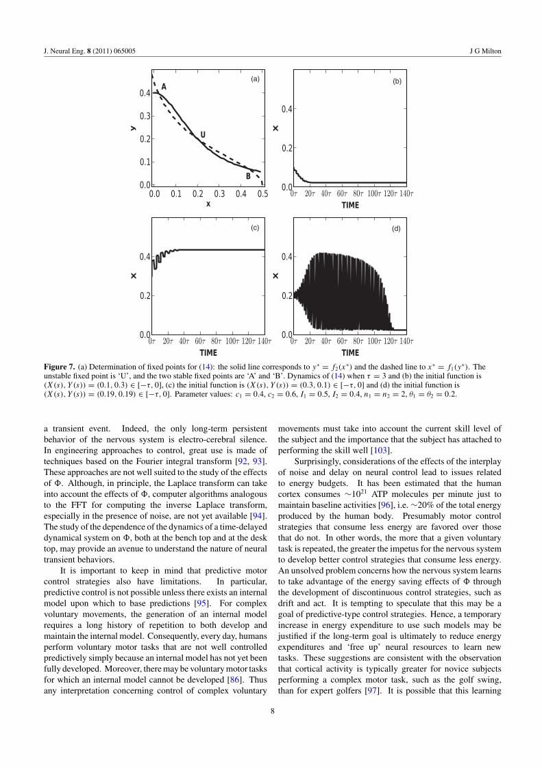
where c, n, θ are positive constants. For appropriate choicesof the parameters, three fixed points coexist (figure 7(a)): twoof these are stable and they are separated by an unstable fixedpoint. It is helpful to think of the two stable fixed points astwo decisions, A and B. Which of the attractors is attaineddepends on the choice of the initial functions, �(x) and �(y).When the functions lie within the basin of attraction of A, weget decision A (figure 7(b)), and when they lie in the basin ofattraction of B, we get decision B (figure 7(c)). However, when�(x) and �(y) are chosen close to the unstable fixed point(U), we get a different and unexpected dynamical behavior,namely a DITO. The duration of the DITO scales exponentiallywith the delay [88] (for example, when τ = 8, the DITOduration is ∼1000τ [48]) and is robust in the presence of noisyperturbations (A Quan, I Osorio and J Milton, unpublishedobservations). In the context of decision making, DITOsrepresent a decision maker who wavers between two decisionsbefore making a decision.

These observations suggest that the nervous system isanticipated to be particularly susceptible to the generationof oscillatory transients at times when changes in stateoccur. This is because as one attractor forms while theother disappears, there is necessarily an interval in time whenboth attractors coexist. Moreover, as this process evolves,the trajectories are drawn toward the separatrix. It has beensuggested that this mechanism might lie at the basis of seizureoccurrence in patients with a rare familial form of epilepsyknown as frontal lobe nocturnal epilepsy [90]. In thesepatients, seizures occur only when the subject is sleeping andare most common during the transition between stage I andstage II sleep.

6. Discussion

It is not possible to ignore the presence of a time delay. Onecannot approximate the dynamics of an infinite-dimensionalsystem by a low-dimensional system without losing potentiallyimportant information. A key point is that a time-delayeddynamical system has memory of its past. This memory entersthe dynamics through the effects of the initial function, �.Finally, for many choices of f , the dynamics of (1) evolveirreversibly in time when τ > 0 [33, 91].

Transient dynamics are an important feature of time-delayed dynamical systems [48, 52, 88, 89]. Concepts ofstability, the basic mathematical tool for the analysis of neuralcontrol mechanisms, emphasize the long time behavior of adynamical system. However, the living nervous system isall about transients: attention abruptly shifts, people fidget,tremors wax and wane; even an epileptic seizure represents

7

J. Neural Eng. 8 (2011) 065005 J G Milton

(a) (b)

(c) (d)

Figure 7. (a) Determination of fixed points for (14): the solid line corresponds to y∗ = f2(x∗) and the dashed line to x∗ = f1(y

∗). Theunstable fixed point is ‘U’, and the two stable fixed points are ‘A’ and ‘B’. Dynamics of (14) when τ = 3 and (b) the initial function is(X(s), Y (s)) = (0.1, 0.3) ∈ [−τ, 0], (c) the initial function is (X(s), Y (s)) = (0.3, 0.1) ∈ [−τ, 0] and (d) the initial function is(X(s), Y (s)) = (0.19, 0.19) ∈ [−τ, 0]. Parameter values: c1 = 0.4, c2 = 0.6, I1 = 0.5, I2 = 0.4, n1 = n2 = 2, θ1 = θ2 = 0.2.

a transient event. Indeed, the only long-term persistentbehavior of the nervous system is electro-cerebral silence.In engineering approaches to control, great use is made oftechniques based on the Fourier integral transform [92, 93].These approaches are not well suited to the study of the effectsof �. Although, in principle, the Laplace transform can takeinto account the effects of �, computer algorithms analogousto the FFT for computing the inverse Laplace transform,especially in the presence of noise, are not yet available [94].The study of the dependence of the dynamics of a time-delayeddynamical system on �, both at the bench top and at the desktop, may provide an avenue to understand the nature of neuraltransient behaviors.

It is important to keep in mind that predictive motorcontrol strategies also have limitations. In particular,predictive control is not possible unless there exists an internalmodel upon which to base predictions [95]. For complexvoluntary movements, the generation of an internal modelrequires a long history of repetition to both develop andmaintain the internal model. Consequently, every day, humansperform voluntary motor tasks that are not well controlledpredictively simply because an internal model has not yet beenfully developed. Moreover, there may be voluntary motor tasksfor which an internal model cannot be developed [86]. Thusany interpretation concerning control of complex voluntary

movements must take into account the current skill level ofthe subject and the importance that the subject has attached toperforming the skill well [103].

Surprisingly, considerations of the effects of the interplayof noise and delay on neural control lead to issues relatedto energy budgets. It has been estimated that the humancortex consumes ∼1021 ATP molecules per minute just tomaintain baseline activities [96], i.e. ∼20% of the total energyproduced by the human body. Presumably motor controlstrategies that consume less energy are favored over thosethat do not. In other words, the more that a given voluntarytask is repeated, the greater the impetus for the nervous systemto develop better control strategies that consume less energy.An unsolved problem concerns how the nervous system learnsto take advantage of the energy saving effects of � throughthe development of discontinuous control strategies, such asdrift and act. It is tempting to speculate that this may be agoal of predictive-type control strategies. Hence, a temporaryincrease in energy expenditure to use such models may bejustified if the long-term goal is ultimately to reduce energyexpenditures and ‘free up’ neural resources to learn newtasks. These suggestions are consistent with the observationthat cortical activity is typically greater for novice subjectsperforming a complex motor task, such as the golf swing,than for expert golfers [97]. It is possible that this learning

8

J. Neural Eng. 8 (2011) 065005 J G Milton

process is accomplished, at least in part, by tuning of thresholdsand modification of conduction delays [98–100] mediated bychanges in axonal myelination [101, 102]. Thus, an importantproblem will be to identify the nature of the cost functions thatthe nervous system uses to manage its resources.

Acknowledgments

The author acknowledges useful discussions with M C Mackeyand Toru Ohira during the preparation of this manuscript. Thiswork was supported by the William R Kenan, Jr Foundationand the National Science Foundation (NSF-1028970).

Appendix. Construction of discontinuous feedback

There are many ways in which F can be constructed. I choseto construct F using two sigmoid functions of the form

(a + b) − b

1 + exp(±q(x(t − τ) − θ)),

where a, b, q are constants. It is convenient to make time anddisplacement dimensionless so that

F(X(T − 1))

=⎧⎨⎩

(A + B) − B1+exp[Q(X(T −1)−1)] if X(T − 1) < T h′

(A + B) − B1+exp[−Q(X(T −1)−T h)] if X(T − 1) � T h′,

where T = t/τ , A = aτ , B = bτ , X = x/θ1, Q = q/θ1,k = (k′τ)/θ1, f = f ′τ , T h = θ2/θ1 and T h′ = (1 + T h)/2.With these definitions, (7) becomes

dX

dT= F(X(T − 1))X(t) + kX(T ) sin 2πf T . (A.1)

The advantage of studying (A.1) is that the dynamics can beconveniently investigated in terms of two amplitude-relatedparameters, namely k and T h. In terms of (A.1), theparameters for the simulation in figure 4(b) were A = 0.18,B = −0.24, Q = 100, τ = 1 and T h = 2.0, and in figure4(b) they were A = 0.18, B = −0.24, T h = 1.181, τ = 1,Q = 60, f = 2 and k = 0.005.

References

[1] Kuiken T A, Miller L A, Lipschutz R D, Lock B A,Stubblefield K, Marasso P D, Zhou P and Dumanian G2007 Targeted reinnervation for enhanced prosthetic armfunction in a woman with a proximal amputation: a casestudy Lancet 369 371–80

[2] Suminski A J, Tkach D C, Fagg A H and Hatsopoulos N G2010 Incorporating feedback from multiple sensorymodalities enhances brain–machine interface controlJ. Neurosci. 30 16777–87

[3] Gabbard C P 2004 Lifelong Motor Development 4th edn(New York: Pearson & Benjamin Cummings)

[4] Hick W E 1952 On the rate of gain of information Q. J. Exp.Psychol. 4 11–26

[5] Nijhawan R 2008 Visual prediction: psychophysics andneurophysiology of compensation for time delays Behav.Brain Sci. 31 179–239

[6] Nijhawan R and Wu S 2009 Compensating time delays withneural prediction: are predictions sensory or motor? Proc.Trans. R. Soc. A 367 1063–78

[7] Stark L 1968 Neurological Control Systems: Studies inBioengineering (New York: Plenum)

[8] Desmurget M and Grafton S 2000 Forward modeling allowsfeedback control for fast reaching movements Trends Cogn.Sci. 4 423–31

[9] Kawato M 1999 Internal models for motor control andtrajectory planning. Curr. Opin. Neurobiol. 9 718–27

[10] Wolpert D M and Kawato M 1998 Multiple paired forward andinverse models for motor control Neural Netw. 11 1317–29

[11] Wolpert D M and Ghahramani Z 2000 Computationalprinciples of movement neuroscience Nat. Neurosci.3 1212–7

[12] Mehta B and Schaal S 2002 Forward models in visuomotorcontrol J. Neurophysiol. 88 942–53

[13] Tass P A 1999 Phase Resetting in Medicine and Biology:Stochastic Modelling and Data Analysis (New York:Springer)

[14] Stepan G 1989 Retarded Dynamical Systems (Harlow:Longman)

[15] Landry M, Campbell S A, Morris K and Aquilar C O 2009Delay effects in the human sensory system during balancingPhil. Trans. R. Soc. 367 1195–212

[16] Stepan G 2009 Delay effects in the human sensory systemduring balancing Phil. Trans. R. Soc. A 367 1195–212

[17] Milton J, Cabrera J L, Ohira T, Tajima S, Tonosaki Y,Eurich C W and Campbell S A 2009 The time-delayedinverted pendulum: implications for human balance controlChaos 19 026110

[18] Pikovsky A, Rosenblum M and Kurths J 2001Synchronization: A Universal Concept in NonlinearSciences (New York: Cambridge University Press)

[19] Milton J G 2010 Epilepsy as a dynamic disease: a tutorial ofthe past with an eye to the future Epilepsy Behav. 18 33–44

[20] Osorio I, Frei M G, Sornette D, Milton J and Lai Y-C 2010Epileptic seizures: quakes of the brain? Phys. Rev.E 82 021919

[21] Voss H U 2000 Anticipating chaotic synchronization Phys.Rev. E 61 5115–9

[22] Stepp N 2009 Anticipation in feedback-delayed manualtracking of a chaotic oscillator Exp. Brain Res. 198 521–5

[23] Stepp N and Turvey M T 2008 Anticipating synchronization asan alternative to the internal model Behav. Brain Sci.31 216–7

[24] Morris K 2001 An Introduction to Feedback Controller Design(New York/San Diego: Harcourt Brace/Academic)

[25] Cabrera J L and Milton J G 2002 On–off intermittency in ahuman balancing task Phys. Rev. Lett. 89 158702

[26] Milton J, Townsend J L, King M A and Ohira T 2009Balancing with positive feedback: the case fordiscontinuous control Phil. Trans. R. Soc. A 367 1181–93

[27] Milton J G, Ohira T, Cabrera J L, Fraiser R M, Gyorffy J B,Ruiz F K, Strauss M A, Balch E C, Marin P Jand Alexander J L 2009 Balancing with vibration: a preludefor ‘drift and act’ control PLoS ONE 4 e7427

[28] Milton J G, Cabrera J L and Ohira T 2008 Unstable dynamicalsystems: delays, noise and control Europhys. Lett. 83 48001

[29] Gauthier J–P, Berret B and Jean F 2010 A biomechanicalinactivation principle Proc. Steklov Inst. Math. 268 93–116

[30] Ermentrout B 2002 Simulating, Analyzing, and AnimatingDynamical Systems: A guide to XPPAUT for researchersand students (Philadelphia: SIAM)

[31] MacDonald N 1989 Biological Delay Systems: LinearStability Theory (New York: Cambridge University Press)

[32] Erneux T 2009 Applied Delay Differential Equations (NewYork: Springer)

[33] Smith H 2010 An Introduction to Delay Differential Equationswith Applications to the Life Sciences (New York: Springer)

[34] Boulet J, Balasubramiam R, Daffertshofer A and Longtin A2010 Stochastic two-delay differential model of delayed

9

J. Neural Eng. 8 (2011) 065005 J G Milton

visual feedback effects on postural dynamics Phil. Trans. R.Soc. A 368 423–38

[35] Eurich C W, Mackey M C and Schwegler H 2002 Recurrentinhibitory dynamics: the role of state-dependentdistributions of conduction delays times J Theor. Biol.216 31–50

[36] Lockhart D B and Ting L H 2007 Optimal sensorimotortransformation of balance Nature Neurosci. 10 1329–36

[37] Foss J, Moss F and Milton J G 1997 Noise, multistability anddelayed recurrent loops Phys. Rev. E. 55 4536–43

[38] Foss J and Milton J 2000 Multistability in recurrent neuralloops arising from delay J. Neurophysiol. 84 975–85

[39] Ma J and Wu J 2007 Multistability in spiking neuron models ofdelayed recurrent inhibitory loops Neural Comp. 19 2124–48

[40] Glass L, Beuter A and Larocque D 1988 Time delays,oscillations, and chaos in physiological control systemsMath. Biosci. 90 111–25

[41] Glass L and Malta C P 1990 Chaos in multilooped negativefeedback systems J. Theor. Biol. 145 217–33

[42] Bastos de Figueiredo J D, Dambia L, Glass L and Malta C P2002 Chaos in two-loop negative feedback systems Phys.Rev. E 65 051905

[43] Judd K T and Aihara K 1993 Pulse propagation networks: aneural network model that uses temporal coding by actionpotentials Neural Netw. 6 203–15

[44] Haken H 2002 Brain Dynamics: Synchronization of ActivityPatterns in Pulse-coupled Neural Nets with Delays andNoise (Berlin: Springer)

[45] Insperger T, Stepan G and Turi J 2010 Delayed feedback ofsampled higher derivatives Phil. Trans. R. Soc. A 368 469–82

[46] Wright E M 1955 A nonlinear differential difference equationJ. Reine Angew. Math. 194 66–87

[47] Guillouzic S, L’Heureux I and Longtin A 1999 Small delayapproximation of stochastic delay differential equationsPhys. Rev. E 59 3970–82

[48] Milton J, Naik P, Chan C and Campbell S A 2010 Indecisionin neural decision making models Math. Model. Nat.Phenom. 5 125–45

[49] Hayes N D 1950 Roots of the transcendental equationassociated with certain difference differential equationsJ. London Math. Soc. 25 226–32

[50] Haller G and Stepan G 1996 Micro-chaos in digital controlJ. Nonlinear Sci. 6 415–48

[51] Seiber J and Krauskopf B 2004 Complex balancing motions ofan inverted pendulum subject to delayed feedback controlPhysica D 197 332–45

[52] Csernak G and Stepan G 2005 Life expectancy of transientmicrochaotic behavior J. Nonlin. Sci. 15 63–91

[53] Lasota A and Mackey M C 1994 Chaos, Fractals, and Noise:Stochastic Aspects of Dynamics 2nd edn (New York:Springer)

[54] Newell K M, Slobounov S M, Slobounova E S andMolenaar P C M 1997 Stochastic processes in posturalcenter-of–pressure profiles Exp. Brain Res. 113 158–64

[55] Frank T D and Beek P J 2001 Stationary solutions of linearstochastic delay differential equations: applications tobiological systems Phys. Rev. E 64 021917

[56] Frank T D 2005 Delayed Fokker–Planck equations, Novikov’stheorem, and Boltzmann distributions as small delayapproximations Phys. Rev. E 72 011112

[57] Ohira T and Milton J G 1995 Delayed random walks Phys.Rev. E 52 3277–80

[58] Ohira T and Yamane T 2000 Delayed stochastic systems Phys.Rev. E 61 1247–57

[59] Ohira T and Milton J 2009 Delayed random walks:investigating the interplay between delay and noise DelayDifferential Equations: Recent Advances and NewDirections ed B Balachandran, T Kalmar–Nagy andD E Gilsinn (New York: Springer) pp 305–35

[60] Mergenthaler K and Enghert R 2007 Modeling the control offixational eye movements with neurophysiological delaysPhys. Rev. Lett. 98 138104

[61] Kamimura A and Ohira T 2010 Group chase and escape NewJ. Phys. 12 053013

[62] Ohira T and Sato Y 1999 Resonance with noise and delayPhys. Rev. Lett. 82 2811–5

[63] Flugge-Lotz I 1968 Discontinuous and Optimal Control (New York: McGraw-Hill)

[64] Hoffmann E R 1992 Fitts law with transmission delayErgonomics 35 37–48

[65] Stepan G and Insperger T 2006 Stability of time-periodic anddelayed systems a route to act-and-wait control Ann. Rev.Control 30 159–68

[66] Insperger T 2006 Act-and-wait concept for continuous-timecontrol systems with feedback delay IEEE Trans. ControlSyst. Technol. 14 974–7

[67] Gawthrop P, Lakie M and Loram I 2008 Predictive feedbackcontrol and Fitts law Biol. Cybern. 98 229–38

[68] Miall R C, Weir D J and Stein J F 1985 Visuomotor trackingwith delayed visual feedback Neuorsci. 16 511–20

[69] Miall RC 1996 Task-dependent changes in visual feedbackcontrol: a frequency analysis of human manual trackingJ. Motor Behav. 28 125–35

[70] Gross J, Timmermann L, Kujala J, Dirks M, Schmitz F,Salmelin R and Schnitzler A 2002 The neural basis ofintermittent motor control in humans Proc. Natl Acad. Sci.USA 99 2299–302

[71] Loram I D and Lakie M 2002 Human balancing of an invertedpendulum: position control by small, ballistic-like, throwand catch movements J. Physiol. 540 1111–24

[72] Loram I D, Maganaris C N and Lakie M 2005 Human posturalsway results from frequent, ballistic bias impulses by soleusand gastrocnemius J. Physiol. 564 295–311

[73] Loram I D, Gollee H, Lakie M and Gawthrop P 2011 Humancontrol of an inverted pendulum: Is continuous controlnecessary? Is intermittent control effective? Is intermittentcontrol physiological? J. Physiol. 589 307–24

[74] Todorov E and Jordan M I 2002 Optimal feedbackcontrol as theory of motor coordination Nat. Neurosci.5 1226–35

[75] Todorov E 2004 Optimality principles in sensorimotor controlNat. Neurosci. 7 907–15

[76] Eurich C W and Milton J G 1996 Noise-induced transitions inhuman postural sway Phys. Rev. E 54 6681–4

[77] Bottaro A, Yasutake Y, Nomura T, Casidio M and Morasso P2008 Bounded stability of the quiet standing posture: anintermittent control model Hum. Mov. Sci. 27 473–95

[78] Asai Y, Tasaka Y, Nomura K, Casidio M and Morasso P 2009A model of postural control in quiet standing: robustcompensation of delay-induced instability using intermittentactivation of feedback control PLoS ONE 4 e6169

[79] Guckenheimer J 1995 A robust hybrid stabilization strategyfor equilibria IEEE Trans. Autom. Control 40 321–6

[80] Shumway-Cook A and Woollacott M H 2001 Motor Control:Theory and Practical Applications 2nd edn (New York:Williams and Wilkins)

[81] Milton J, Gyorffy J, Cabrera J L and Ohira T 2010 Amplitudecontrol of human postural sway using Achilles tendonvibration 16th US National Congress of Theoretical andApplied Mechanics (State College, PA)

[82] Insperger T 2011 Stick balancing with reflex delay in case ofparametric forcing Commun. Nonlinear Sci. Numer. Simul.16 2160–8

[83] Orban G, Vandenbussche E and Vogels R 1984 Humanorientation discrimination tested with long stimuli VisionRes. 24 121–8

[84] Dodson M J, Goodwin A W, Browning A S and Gehring H M1998 Peripheral neural mechanisms determining the

10

J. Neural Eng. 8 (2011) 065005 J G Milton

orientation of cylinders grasped by digits J. Neurosci.18 521–30

[85] Acheson D 1998 From Calculus to Chaos: An Introduction toDynamics (New York: Oxford University Press)

[86] Venkadesan M, Guckenheimer J and Valero-Cuevas F J 2007Manipulating the edge of stability J. Biomech. 40 1653–61

[87] Pyragas K and Pyragas T 2010 Extending anticipation horizonof chaos synchronization schemes with time-delay couplingPhil. Trans. R. Soc. A 368 305–17

[88] Pakdaman K, Grotta-Ragazzo C and Malta C P 1998 Transientregime duration in continuous-time neural networks withdelay Phys. Rev. E 58 3623–7

[89] Grotta–Ragazzo C, Pakdaman K and Malta C P 1999Metastability for delayed differential equations Phys. Rev.E 60 6230–3

[90] Milton J G, Quan A and Osorio I 2011 Nocturnal frontal lobeepilepsy: metastability in a dynamic disease? Epilepsy:The Intersection of Neurosciences, Biology, Mathematics,Engineering and Physics ed I Osorio, H P Zanvari,M G Frei and S Arthurs (New York: CRC Press, Taylor andFrancis) pp 501–10

[91] Mackey M C 1998 Time’s Arrow: The Origins ofThermodynamic Behavior (New York: Springer)

[92] James H M, Nichols N B and Phillips R S 1965 Theory ofServomechanisms (New York: Dover)

[93] Astrom K J and Murray R M 2008 Feedback Systems: AnIntroduction for Scientists and Engineers (Princeton, NJ:Princeton University Press)

[94] Epstein C E and Schotland J 2008 The bad truth aboutLaplace’s transform SIAM Rev. 50 504–20

[95] Valero-Cuevas F J, Hoffman H, Kurse M U, Kutch J Jand Theodorou E A 2009 Computational models forneuromuscular function IEEE Rev. Biomed. Eng.2 110–35

[96] Lennie P 2003 The cost of cortical computation Curr. Biol.13 493–7

[97] Milton J, Solodkin A, Hlustik P and Small S L 2007 The mindof expert motor performance is cool and focusedNeuroImage 35 804–13

[98] Hebb D O 1949 The Organization of Behavior (New York:Wiley)

[99] Eurich C W, Pawelzik K, Ernst U, Cowan J D and Milton J G1999 Dynamics of self-organized delay adaptation Phys.Rev. Lett. 82 1594–7

[100] Wu J, Zivari–Piran H, Hunter J D and Milton J G 2011Projective clustering using neural networks withadaptive delay and signal transmission loss Neural Comp.23 1568–604

[101] Stevens B, Tanner S and Fields R D 1998 Control ofmyelination by specific patterns of neural impulsesJ. Neurosci. 18 9303–11

[102] Fields R D 2005 Myelination: an overlooked mechanism ofsynaptic plasticity? Neuroscientist 11 528–31

[103] Milton J, Small S L and Solodkin A 2008 Imaging motorimagery: methodological issues related to expertiseMethods 45 336–41

11