the demand for divisia money: theory and evidence demand for divisia money: theory and evidence ......
TRANSCRIPT
The Demand for Divisia Money: Theory and Evidence
Michael T. Belongia Otho Smith Professor of Economics
University of Mississippi Box 1848
University, MS 38677 [email protected]
Peter N. Ireland Department of Economics
Boston College 140 Commonwealth Avenue
Chestnut Hill, MA 02467 [email protected]
November 2017
Abstract: A money-in-the-utility function model is extended to capture the distinct roles of noninterest-earning currency and interest-earning deposits in providing liquidity services to households. It implies the existence of a stable money demand relationship that links a Divisia monetary aggregate to spending or income as a scale variable and the associated Divisia user-cost dual as an opportunity cost measure. Cointegrating money demand equations of this form appear in quarterly United States data spanning the period from 1967:1 through 2017:2, especially for the Divisia M2 aggregate. The identification of a stable money demand function over a period that includes the financial innovations of the 1980s and continues through the recent financial crisis and Great Recession suggests that a properly measured aggregate quantity of money can play a role in the conduct of monetary policy. That role can be of greater prominence when traditional interest rate policies are constrained by the zero lower bound. JEL Codes: C43, E41. Keywords: Divisia monetary aggregates, money demand, money-in-the-utility function. Acknowledgments: Neither of us received any external support for, or has any financial interest that relates to, the research described in this paper.

1
Introduction
Since Milton Friedman’s (1956) “restatement,” the existence of a stable money demand
function has been regarded as a necessary pre-condition for the success of any quantity-
theoretic approach to monetary policy that would use information in broad monetary
aggregates to achieve goals for aggregate spending or the price level. The general message of
Friedman’s essay, supported by the empirical papers that accompanied its publication,
motivated a broad and active line of research in monetary economics that lasted more than
three decades.1 The primary focus of this agenda was the search for statistical relationships
that linked the demand for real money balances to a small number of determinants, especially
income or spending and interest rates. By the end of the 1970s, considerable evidence had
been assembled to support the notion of a stable demand for money function and, when
inflation had risen to increasingly higher rates, this evidence provided the foundation for a
monetary policy strategy based on intermediate targets for growth rates of the money supply.
Interest in the demand for money, however, quickly waned in the early 1990s,
beginning with the publication of highly influential studies by Bernanke and Blinder (1992)
and Friedman and Kuttner (1992). Those studies showed that previously stable relationships
between money and other key macroeconomic variables – including popular money demand
specifications – weakened considerably after 1980. Moreover, their results indicated that any
significant effects of monetary policy actions on aggregate activity were manifested through
changes in the federal funds rate rather than the quantity of money.2 Conventional wisdom
held that sweeping financial innovations during the 1980s permanently altered whatever
associations might have been found in the data of the 1960s and 70s. Although the findings in
these studies and others like them subsequently were shown by Belongia (1996) and, more
recently, Hendrickson (2014), to depend partly on their use of the Federal Reserve’s simple-
sum monetary aggregates instead of the Divisia alternatives proposed by Barnett (1980), they
nevertheless had led a professional consensus to coalesce around the idea that measures of
money could be safely excluded from the information set used to evaluate the effects of
monetary policy on economic activity or to assess the relative ease or tightness of policy at a
moment in time.
About the same time, John Taylor also shifted his focus from money to interest rates.
Having earlier (Taylor 1979) investigated the properties of a monetary policy rule based on 1 Friedman’s essay and the accompanying papers appeared in Studies in the Quantity Theory of Money (1956). Laidler (1993) provides a survey of the research on the demand for money that followed. 2 A related issue, also associated with measurement of the money supply, was the so-called “velocity problem.” For example, the sharp decline in the velocity of M2 (a shift in the demand for M2) after the financial innovations of the 1980s quickly undercut the perceived usefulness of the P-Star model of Hallman, Porter, and Small (1991).

2
money, he now (Taylor 1993) suggested that Federal Reserve policy, beginning in the late
1980s, could be adequately described by a strikingly simple alternative based on the federal
funds rate. Notably, this rule called for adjustments in the federal funds rate in response to
movements in inflation and output alone with no separate role for the money supply. Interest
rate rules of the general form proposed by Taylor then were incorporated into the New
Keynesian models developed by Clarida, Galí, and Gertler (1999) and Woodford (2003). And
though Nelson (2008) and even Taylor (1996) himself showed that New Keynesian models with
interest rate rules are not inconsistent with the quantity-theoretic view that inflation gets
determined, in the long run, by the growth rate of the money supply, these models also served
to illustrate how monetary policy analysis could be conducted within a theoretically coherent
and internally consistent framework that makes no explicit reference to either the demand for
or supply of money. As such, models of this type also excluded any independent transmission
mechanism by which variations in the quantity of money can affect real activity independent of
any influence associated with variations in interest rates.
Recent events, however, provide good reason to reconsider the role of the monetary
aggregates in monetary policy analysis. Most significantly, the zero lower bound on nominal
interest rates, which became a binding constraint on the Federal Reserve’s interest rate policy
over an extended period from 2008 through 2015, highlights the limitations of any approach
that uses the federal funds rate alone to gauge the stance of monetary policy. If, for example,
Federal Reserve actions affect spending and prices through changes in variables other than the
funds rate, these effects will not be captured by models that exclude, by construction, any
channel of monetary transmission apart from an interest rate. In fact, empirical evidence
shows how Divisia monetary aggregates can be used within structural vector autoregressive
time series models to help identify monetary policy shocks before and during the period of zero
nominal interest rates by capturing the consequences of “unconventional” policy actions such
as large-scale asset purchases or “quantitative easing” through their effects on the growth rate
of Divisia money.3 Because the results from these studies are consistent with the ideas that
helped motivate the money demand research agenda sixty years ago, these same Divisia
monetary aggregates might be used to estimate stable money demand relationships of the kind
envisioned by Friedman (1956). If identified, these relationships then could serve as the
foundations for a quantity-theoretic approach to monetary policymaking and analysis that
downplays the significance of the zero lower bound, yet also works reliably to stabilize inflation
during normal periods with positive nominal interest rates.
To explore this possibility, this paper begins by modifying Lucas’ (2000) version of the
money-in-the-utility function model, developed originally by Sidrauski (1967) and Brock (1974), 3 See, for example, Keating, Kelly, Smith, and Valcarcel (2014) and Belongia and Ireland (2015b, 2016, 2017),

3
by introducing separate roles for noninterest-earning currency and interest-earning deposits in
providing a representative household with liquidity services that allow it to purchase goods and
services at the expense of less time and effort. This extension to the theory makes clear that
the money demand relationship implied by the model applies to a Divisia monetary aggregate
but not a simple-sum measure of the type provided officially by the Federal Reserve. The same
theoretical extension also reinforces Belongia’s (2006) argument that the price, or user-cost,
dual to the Divisia monetary aggregate ought to appear in place of a short-term nominal
interest rate as a preferred opportunity cost measure in the money demand equation. Finally,
the extended money-in-the-utility function model can be used to motivate renewed interest in
classic empirical specifications for money demand, originally proposed by Cagan (1956), Selden
(1956), Latané (1960), and Meltzer (1963), adapted to apply to the Divisia monetary aggregates
instead of the standard simple sum measures.
The paper goes on to estimate these money demand equations using Johansen’s (1991)
maximum likelihood approach together with quarterly data on the Divisia aggregates described
by Barnett, Liu, Mattson, and van den Noort (2013) and made available through the Center for
Financial Stability’s (CFS) website. In both the full sample of data running from 1967:1
through 2017:2 and a subsample beginning in 1983:1, cointegrating money demand
relationships of the form suggested by the theory link the Divisia monetary aggregates to either
spending or income as a scale variable and the associated Divisia user cost aggregate as an
opportunity cost measure. Estimates of the elasticity of Divisia money demand with respect to
changes in the user cost decline when estimated with data from the post-1983 subsample,
relative to the full sample. But the long-run money demand relationships appear most
consistently for the Divisia M2 aggregate, implying that a monetary policy strategy focused on
stabilizing Divisia M2 growth has the potential to stabilize the aggregate price level or its rate of
change.4
By using the most recent data to estimate statistical money demand equations, this
paper joins with a few others, including Judson, Schlusche, and Wong (2014), Lucas and
Nicolini (2015), and Anderson, Bordo, and Duca (2017), that also are motivated by the financial
crisis and period of zero nominal interest rates to reconsider a more traditional, quantity-
theoretic approach to monetary policy analysis. Meanwhile, Benati, Lucas, Nicolini, and Weber
(2016) and Benati (2017) revive the analysis of long-run money demand by estimating these
equations using international data extending back, in some cases, to the 19th century.
Likewise, Serletis and Gogas (2014) estimate long-run money demand relationships for the CFS
Divisia aggregates, but use the three-month United States Treasury bill rate as their
4Belongia and Ireland (2015a) present evidence on the viability of targeting a path for nominal GDP by controlling the behavior of a Divisia monetary aggregate, a result suggestive of a stable demand for money function.

4
opportunity cost measure. Because the theory suggests, however, that the “price” of monetary
services is the user cost dual to the economic quantity aggregate, the empirical specifications
that follow use this measure instead. The results presented here, therefore, provide evidence of
stable money demand relationships based on price and quantity data derived from the same
principles.
Theory
The Model
As noted above, the model developed here builds further on Lucas’ (2000) variant of the
money-in-the-utility function models of Sidrauski (1967) and Brock (1974) by introducing
separate roles for noninterest-earning currency and interest-earning deposits in providing a
representative household with liquidity services that allow it to purchase goods and services
with less effort. Through this extension, the theory makes clear that the aggregate of currency
and deposits appearing in a properly-specified money demand relationship is a Divisia
aggregate, and not simple sum measures like those constructed, officially, by the Federal
Reserve. While the description of household optimization provided here could be incorporated
into a dynamic, stochastic, general equilibrium model along the same lines followed by
Belongia and Ireland (2014) and Ireland (2014), the perfect foresight, partial equilibrium
framework used here, instead, simplifies the analysis by abstracting from unnecessary general
equilibrium considerations and highlights, as well, that the basic properties of the money
demand relationship derived here do not depend on the details of how other sectors of the
economy might be modeled.
Also for simplicity, the theoretical analysis proceeds here under the assumption that a
representative household substitutes between currency and a single type of interest-earning
bank deposit in its efforts to construct the portfolio of these two liquid assets that most
efficiently provides the monetary services it uses in making transactions during each period.
Additional types of deposits, all paying interest at different rates and each playing its own role
in the household’s portfolio of monetary assets, could easily be incorporated, at the cost of
requiring slightly more detailed notation and more tedious algebra. The empirical work, by
contrast, uses various Divisia monetary aggregates that do include a wide range of monetary
assets available in the United States today.
In the model, an infinitely-lived representative household enters each period
0,1,2,...t = with 1tM − units of currency and 1tB − bonds. At the very start of a beginning-of-
period asset trading and allocation session, the household receives tT additional units of
currency. Next, the household’s bonds mature, providing 1tB − more units of currency. The

5
household uses some of its currency to purchase tB new bonds at the price of 1/ (1 )tr+
dollars per bond, where tr denotes the net nominal interest rate between t and 1t + . The
household divides its remaining currency into an amount tN to be used for transactions
purposes during the period and an amount to be deposited in an interest-earning bank
account instead. At the same time, the household also borrows tL dollars from the bank,
which then gets credited to its bank account. Thus, the total value tD of the household’s
deposits must satisfy
Mt−1 +Tt + Bt−1 −
Bt
1+ rt
− Nt + Lt ≥ Dt (1)
for all 0,1,2,...t = .
To describe its activities following this initial asset allocation session, it is helpful to
follow Lucas (1980) by imagining that the representative household consists of two members: a
worker and a shopper. During each period 0,1,2,...t = , the representative household’s worker
supplies labor inelastically to produce ty units of output, where ty may fluctuate or grow over
time, reflecting any arbitrary pattern of exogenous technological change, so long as it is
anticipated in line with the perfect foresight assumption. The worker then sells this output to
shoppers from other households at the nominal price of tP dollars per unit of the good. The
representative household’s shopper, meanwhile, purchases tc units of the good at the same
price tP from workers of other households.
At the end of each period 0,1,2,...t = , the household’s two members reunite to
consume the shopper’s purchases. The household’s preferences over the infinite horizon are
described by the utility function
1
0
1 1 ,1
at t
tt t t
Mc vPc
σ
βσ
−∞
=
⎧ ⎫⎡ ⎤⎛ ⎞⎪ ⎪⎛ ⎞ −⎨ ⎬⎢ ⎥⎜ ⎟⎜ ⎟−⎝ ⎠ ⎝ ⎠⎣ ⎦⎪ ⎪⎩ ⎭∑ (2)
where the discount factor lies between zero and one, so that 0 1β< < , and the intertemporal
elasticity of substitution parameter is positive, so that 0σ > . In the special case where 1σ = ,
the single-period utility function in (2) should be understood to take its limiting form
ln( ) ln .at
tt t
Mc vPc
⎡ ⎤⎛ ⎞+ ⎢ ⎥⎜ ⎟
⎝ ⎠⎣ ⎦

6
In (2), the function v captures the time-and-effort-saving services provided to the
representative household’s shopper by the monetary aggregate atM , formed from currency and
deposits according to
( , ) ,at t tg N D M≥
where the monetary aggregator g is assumed to be homogeneous of degree one, so that the
underlying transaction technology exhibits constant returns to scale and so that this
constraint can be rewritten equivalently in real terms as
,a
t t t
t t t
N D MgP P P
⎛ ⎞≥⎜ ⎟
⎝ ⎠ (3)
for all 0,1,2,...t = . As noted by Lucas (2000), the specific form of the utility function in (2)
makes the model consistent with balanced growth: if the household’s real income ty grows at a
constant long-run growth rate, then its optimal choices of consumption tc and the real
monetary aggregate /at tM P will grow at the same long-run rate.
The specification in (3) allows for a wide range of possibilities regarding the degree of
substitutability between currency and deposits in providing the household with monetary
services. Belongia and Ireland (2014) and Ireland (2014) assume, for example, that g takes
the constant elasticity of substitution form
1/ ( 1)/ 1/ ( 1)/ /( 1)( , ) [ (1 ) ] ,t t t tg N D N Dω ω ω ω ω ω ω ων ν− − −= + −
with 0ω > and 0 1ν< < . Here, this CES function could serve as a special case, but the
analysis applies more generally to any aggregator g satisfying the homogeneity assumption
that doubling the quantities of currency and deposits held also doubles the monetary services
produced by the combination of these underlying assets. Note, however, that another special
case,
( , ) ,t t t tg N D N D= +
also is subsumed under the more general formulation allowed for in (3) and is consistent with
the official practice of constructing monetary aggregates as the “simple sums” of funds held as
currency and deposits. It implies, however, that so long as deposits pay interest while
currency does not, the household will choose a corner solution in which it holds only deposits
and no currency. In economies, including the United States’, where households are observed
to hold both currency and deposits, this simple-sum aggregator appears far less plausible than
others in which currency and deposits substitute imperfectly for one another in providing
monetary services. This is the same point made originally by Barnett (1980): unless currency
and deposits are treated, counterfactually, as perfect substitutes, simple-sum monetary

7
aggregation is inconsistent with economic theory, and simple-sum monetary aggregates are
unlikely to measure accurately the true flows of monetary services demanded by households.
Also at the end of each period 0,1,2,...t = , the household receives an interest payment
dt tr D on the deposits it holds during the period, but must also repay with interest l
t tr L the
loans it received earlier from the bank. After accounting for these receipts and payments, as
well as the income t tP y earned and funds t tPc spent during the period, the household carries
tM units of currency into period 1t + , where
(1 ) (1 )d lt t t t t t t t t tN r D P y Pc r L M+ + + − − + ≥ (4)
for all 0,1,2,...t = . The household, therefore, chooses tB , tN , tD , tL , tc , atM , and tM for all
0,1,2,...t = to maximize the utility function in (2) subject to the constraints in (1), (3), and (4),
each of which must hold for all 0,1,2,...t = .
The most convenient way of characterizing the solution to the household’s problem
starts by rewriting the constraints from (1) and (4) in real terms, as
1 1 / (1 )t t t t t t t t
t t
M T B L B r N DP P
− −+ + + + + +≥ (5)
and
(1 ) (1 ) ,
d lt t t t t t
t tt t
N r D r L My cP P
+ + + ++ ≥ + (6)
before introducing 1tΛ , 2
tΛ , and 3tΛ as the nonnegative Lagrange multipliers on (3), (5), and (6).
The first-order conditions for the household’s problem can then be written as
2 2
1
1
,(1 )
t t
t t tP r Pβ +
+
Λ Λ=+
(7)
1 2 31 , ,t t
t t tt t
N DgP P
⎛ ⎞Λ = Λ −Λ⎜ ⎟
⎝ ⎠ (8)
1 2 32 , (1 ) ,dt t
t t t tt t
N Dg rP P
⎛ ⎞Λ = Λ − + Λ⎜ ⎟
⎝ ⎠ (9)
2 3(1 ) ,lt t trΛ = + Λ (10)
3,a a a at t t t
t tt t t t t t t t
M M M Mc v v vPc Pc Pc Pc
σ−⎡ ⎤ ⎡ ⎤⎛ ⎞ ⎛ ⎞ ⎛ ⎞ ⎛ ⎞′− = Λ⎢ ⎥ ⎢ ⎥⎜ ⎟ ⎜ ⎟ ⎜ ⎟ ⎜ ⎟
⎝ ⎠ ⎝ ⎠ ⎝ ⎠ ⎝ ⎠⎣ ⎦ ⎣ ⎦ (11)
8
1,a at t
t tt t t t
M Mc v vPc Pc
σ−⎡ ⎤⎛ ⎞ ⎛ ⎞′ = Λ⎢ ⎥⎜ ⎟ ⎜ ⎟
⎝ ⎠ ⎝ ⎠⎣ ⎦ (12)
and
3 2
1
1
,t t
t tP Pβ +
+
Λ Λ= (13)
together with (3), (5), and (6) as equalities for all 0,1,2...t = .
Monetary Aggregation and Money Demand
Note that (7) and (13) imply
2 3(1 ) .t t trΛ = + Λ (14)
Comparing (10) and (14) then reveals that the absence of arbitrage requires lt tr r= for all
0,1,2,...t = , so that the interest rate on bonds and loans are always equal. This result reflects
the fact that in the model, for simplicity, bonds and loans are both risk-free assets that provide
no monetary services. In considering the monetary aggregates implied by this model, therefore,
either the bond rate or the loan rate serves equally well as the “benchmark” against which the
lower interest rate on deposits and the zero interest rate on currency can be compared in
computing their associated user costs. In the United States’ economy, however, short-term
risk-free bonds – for example, three-month United States Treasury bills – may provide liquidity
services and, indeed, are included in the broadest, Divisia M4 aggregate defined by Barnett,
Liu, Mattson, and van den Noort (2013). By contrast, bank loans are not included in any of the
CFS Divisia monetary aggregates and, according to Barnett, Liu, Mattson, and van den Noort
(2013), an interest rate on commercial and industrial loans serves for much of the sample
period as the benchmark rate in constructing these aggregates. Thus, while neither bonds nor
bank loans play a direct role in this simple model in providing monetary services to households
or borrowed funds to either the government or private firms, both are included in the
household’s problem to point out that the model’s benchmark rate could be either the rate tr
on illiquid bonds or the rate ltr on illiquid bank loans.
Given tr (or ltr ), define a
tr so that
1 3/at t t tr r− = Λ Λ (15)
for all 0,1,2,...t = . Using (14) and (15), it can be verified that if the choices of currency and
deposits are not of independent interest, the household’s problem can be stated more simply as

9
one of choosing tB , tL , tc , atM , and tM for all 0,1,2,...t = to maximize the utility function in
(2) subject to the constraints
1 1 / (1 ) at t t t t t t
t t
M T B L B r MP P
− −+ + + + +≥
and
(1 ) (1 )a a l
t t t t tt t
t t
r M r L My cP P
+ + ++ ≥ +
for all 0,1,2,...t = , confirming that atM can be treated as a true microeconomic aggregate of
monetary services, with “own rate of return” equal to atr . Equation (3) still makes clear,
however, that this true monetary aggregate will not correspond to a simple sum of currency
and deposits, except in the counterfactual case where these assets are perfect substitutes.
Equations (14) and (15) also allow (8) and (9) to be rewritten as
3
1 1,n
t t t t t ta a
t t t t t t
N D r r ugP P r r u
⎛ ⎞ Λ= = =⎜ ⎟ Λ −⎝ ⎠ (16)
and
3
2 1
( ), ,d d d
t t t t t t t ta a
t t t t t t
N D r r r r ugP P r r u
⎛ ⎞ − Λ −= = =⎜ ⎟ Λ −⎝ ⎠ (17)
where the last equalities in each of these expressions use Barnett’s (1978) formula to define the
user costs of currency and deposits as
1
n tt
t
rur
=+
and
1
dd t tt
t
r rur
−=+
and the user cost of the monetary aggregate atM as
.1
aa t tt
t
r rur
−=+
(18)
Using (16) and (17) together with Euler’s theorem, the homogeneity of the monetary
aggregator g can now be seen to imply
1 2, , ,a n dt t t t t t t t t t t t t
a at t t t t t t t t t t t t
M N D N N D D N D u N u Dg g gP P P P P P P P P u P u P
⎛ ⎞ ⎛ ⎞ ⎛ ⎞ ⎛ ⎞ ⎛ ⎞ ⎛ ⎞ ⎛ ⎞= = + = +⎜ ⎟ ⎜ ⎟ ⎜ ⎟ ⎜ ⎟ ⎜ ⎟ ⎜ ⎟ ⎜ ⎟
⎝ ⎠ ⎝ ⎠ ⎝ ⎠ ⎝ ⎠ ⎝ ⎠ ⎝ ⎠ ⎝ ⎠
or, more simply,

10
.a a n dt t t t t tu M u N u D= + (19)
The left-hand side of (19) measures total expenditures on monetary services; the right-hand
side decomposes these expenditures into components provided by currency and deposits.
Although neither of the two terms on the left-hand side, the user cost atu nor the quantity
aggregate atM , is observable individually, all of the terms on the right-hand side are observable
from data on currency, deposits, and the interest rates on deposits and the benchmark, illiquid
asset. Thus, total expenditures on the left-hand side can be inferred from the sum on the
right, and the expenditure shares for currency
n n
n t t t tt a a n d
t t t t t t
u N u Nsu M u N u D
= =+
and for deposits
d d
d t t t tt a a n d
t t t t t t
u D u Dsu M u N u D
= =+
are observable as well.
In practice, therefore, the measurement problem posed by the theory involves
distinguishing between the two terms atu and a
tM on the left-hand side of (19). This problem,
however, is conceptually no different from the one that arises in a national income accounting
exercise whereby nominal GDP is computed as the sum of all dollar spending on finished goods
and services produced in the economy during a given period of time, but must then be broken
down into its two components – real GDP and the aggregate price level – using economic
aggregation and index-number theory. For monetary aggregation, in particular, Barnett (1980,
2012) shows that the discrete-time Divisia approximation
1 11 1 1ln( ) ln( ) [ln( ) ln( )] [ln( ) ln( )]
2 2
n n d da a t t t tt t t t t t
s s s sM M N N D D− −− − −
⎛ ⎞ ⎛ ⎞+ +− ≈ − + −⎜ ⎟ ⎜ ⎟⎝ ⎠ ⎝ ⎠
tracks the true quantity aggregate closely under a wide range of circumstances and,
importantly, does not require knowledge of the form or parameters of the monetary aggregator
function g . Moreover, once a series for atM is constructed using this formula, a
corresponding series for the user cost atu can be computed, as well, based on “factor reversal,”
that is, by dividing total expenditures a at tu M by the quantity index a
tM . This is, in fact, exactly
how the CFS Divisia quantity and user costs are constructed for monetary aggregates that
include currency and a wide range of bank deposits and other highly liquid assets.
Hence, this model provides a theory of the demand for money as measured by a Divisia
aggregate but not a simple sum measure. To see this, combine (11), (12), and (15) to obtain

11
.
at
a t tt t a a a
t t t
t t t t t t
MvPc
r rM M Mv vPc Pc Pc
⎛ ⎞′⎜ ⎟⎝ ⎠− =
⎛ ⎞ ⎛ ⎞ ⎛ ⎞′−⎜ ⎟ ⎜ ⎟ ⎜ ⎟⎝ ⎠ ⎝ ⎠ ⎝ ⎠
(20)
This condition takes the same form as Lucas’ (2000, p.256) equation 3.7, except that atM in
(20) is clearly best measured by a Divisia monetary aggregate and the additional, “own rate”
term atr appears on the left-hand side to account for the interest paid on many forms of bank
deposits. The equation defines, implicitly, a money demand function of the form
( )a
att t
t t
M h r rPc
= − (21)
with unitary scale elasticity and at tr r− as its opportunity cost measure. Equation (18) links
this opportunity cost to the user-cost dual atu of the Divisia quantity aggregate. With regard to
the empirical specifications that follow, Belongia (2006) notes that the Divisia user cost, as a
theoretically-coherent measure of the own-price of monetary services in a money demand
relationship, also implies that an interest rate, which is associated with the price of bonds,
represents the price of a substitute, rather than the opportunity cost of holding money.5
Three Empirical Specifications
Let
a
a tt
t t
MmPc
= (22)
denote the ratio of the real monetary aggregate to consumption spending tc , and invert (21) to
obtain
( ).a at t tr r mψ− =
Then (20) implies that, given ψ , the original utility function v will solve the differential
equation
5 Note that the explicit derivation of money’s own price as the dual to the economic quantity aggregate stands in contrast to the empirical tradition of measuring the opportunity of holding money balances by the ad hoc choice of a short term interest rate, a long rate, an interest rate spread, or a wage rate.

12
( ) ( ) ,( ) 1 ( )
a a
a a av m mv m m m
ψψ
′=
+ (23)
which coincides with Lucas’ (2000, p.257) equation 3.9 except that, again, the functions v and
ψ have, as their arguments, the ratio of a real Divisia monetary aggregate to consumption.
Equations (21) and (23) can be used to specialize the model so that it motivates several
classical empirical formulations for money demand, modified here to relate the demand for a
Divisia monetary aggregate to its associated user cost. Suppose, for example, that the money
demand function (21) takes the “double-log” form proposed by Meltzer (1963):
0 1ln( / ) ln( ) ln( ),a at t t t tM P c r rα α= + − − (24)
so that 1 0α > measures the absolute value of the constant elasticity of real Divisia money
demand with respect to changes in its opportunity cost at tr r− . Equation (23) then can be used
to verify that this specification for money demand is implied by any utility function of the form
1 1
1 1
/(1 )
0 1(1 )/
exp( / )( ) 1 ,( )
aav mm
α α
α αα αα
− −
−
⎡ ⎤= +⎢ ⎥⎣ ⎦
with 0α > . Alternatively, if (21) takes the “semi-log” form proposed by Cagan (1956),
0 1ln( / ) ln( ) ( ),a at t t t tM P c r rδ δ= + − − (25)
where 1 0δ > measures the absolute value of the constant semi-elasticity of real Divisia money
demand with respect to the opportunity cost, (23) requires that
0
1 0
( ) ln( ) .( ) ln( )
a a
a a a av m mv m m m m
δδ δ
′ −=+ −
This differential equation lacks a closed-form solution, but for any specific values of 0δ and 1δ
obtained by estimating (25), ( )av m can be characterized by solving it numerically.
Ireland (2009) estimates money demand functions of the double-log and semi-log forms
(24) and (25) using data on simple-sum M1 and the three-month United States Treasury bill
rate. More recently, Benati, Lucas, Nicolini, and Weber (2016) and Benati (2017) use long-run
data on simple-sum M1, augmented for the period since 1980 by adding balances from money
market deposit accounts, to estimate another classic money demand specification, first
proposed by Selden (1956) and Latané (1960). When applied to simple-sum aggregates, this
specification posits a linear relationship between monetary velocity and a short-term nominal
interest rate. Here, the same specification is adapted for use with the Divisia monetary
aggregates by letting

13
a t tt a
t
PcvM
= (26)
denote the consumption velocity of atM and assuming that (21) implies
0 1( ),a at t tv r rγ γ= + − (27)
where the parameter 1 0γ > measures the constant responsiveness of Divisia monetary velocity
to changes in the opportunity cost measure. In this case, (23) has a solution of the form
1 1 11/(1 ) /(1 )0 1( ) ( ) ( 1 ) ,a a av m m mγ γ γγ γ γ+ += − −
with 0γ > .
Thus, depending on the specific form of the utility function v , the model presented here
is consistent with any of the classic money demand functions (24), (25), or (27). The next
section presents estimates of these three money demand equations, based on United States
data on Divisia monetary aggregates and their associated user costs.
Evidence
Overview of the Data
Figures 1 and 2 illustrate the behavior of the four variables appearing in the three
Divisia money-demand specifications (24), (25) and (27): the natural logarithm of the ratio of a
Divisia monetary aggregate atM to nominal personal consumption expenditures t tPc , the
natural logarithm and the level of the associated opportunity cost measure at tr r− , and the
consumption velocity of money computed by dividing nominal personal consumption
expenditures by the Divisia monetary aggregate. As noted previously, the series on Divisia
money are described by Barnett, Liu, Mattson, and van den Noort (2013) and made available
through the Center for Financial Stability’s website. Because the theory links money demand
most closely to consumption, personal consumption expenditures is used as the scale variable
in figures 1 and 2 and in generating the benchmark statistical results that follow. Figures and
tables in the appendix show, however, that very similar results and conclusions follow when
nominal GDP is used to scale the data on Divisia money instead. Both series – for nominal
PCE and GDP – are drawn from the Federal Reserve Bank of St. Louis’ FRED database. The
data on aggregate spending and income dictate a quarterly frequency for all series, while the
starting point for the CFS monetary data determines the sample period, running from 1967:1
through 2017:2.
Four levels of monetary aggregation are considered. The Divisia M1 and M2 measures
contain the same assets included in the Federal Reserve’s official, simple-sum aggregates. In
particular, Divisia M1 includes currency, travelers’ checks, demand deposits, and other

14
checkable deposits. Divisia M2 adds savings deposits, including money market deposit
accounts, retail money market mutual fund shares, and small time deposits. The MZM
monetary aggregate, which excludes the small time deposit component of M2 but adds
institutional money market mutual fund shares, was first proposed by Motley (1988) and given
the label “money, zero maturity” by Poole (1991). The CFS data include a Divisia measure at
this level of aggregation as well. Finally, Divisia M4 – the broadest aggregate compiled by the
CFS – combines all of the assets in M2 and MZM with large time deposits, overnight and term
repurchase agreements, commercial paper, and United States Treasury bills to obtain a
collection similar to that included in the Federal Reserve’s discontinued L measure of liquidity.
The CFS also produces user cost aggregates for each of the Divisia quantity aggregates,
constructed via factor reversal by dividing total expenditures on monetary services, measured
according to an extended version of the formula displayed in (19), but with multiple classes of
deposits (and in the case of M4, other highly liquid assets), by the corresponding quantity
aggregate. Because the Divisia user cost of each aggregate is defined and measured according
to the formula in (18), whereas the money demand relationship (21) implied by the theory links
money demand, instead, to the opportunity cost measure at tr r− , each CFS user cost series is
multiplied by 1 tr+ , where tr is the benchmark rate also described by Barnett, Liu, Mattson,
and van den Noort (2013), before use in the statistical analysis. In all of the discussion that
follows, therefore, this measure at tr r− is referred to interchangeably as the “user cost” or
“opportunity cost” of the corresponding Divisia monetary aggregate.
Figure 1 plots each quarterly series in isolation, to illustrate its univariate properties.
The panels in the first column show that at all four levels of aggregation, the log Divisia money-
consumption ratio trends steadily downward during the “Great Inflation” of the 1970s before
leveling off and remaining stable from the early 1980s through the onset of the financial crisis
in 2007-08. Since then, all four Divisia aggregates – but especially M1, M2, and MZM – have
grown more rapidly than spending, generating a new, upward trend in the money-consumption
ratio.
The next two columns of figure 1 plot the opportunity cost variable at tr r− in logs, as it
appears in Meltzer’s (1963) specification (24) and in levels, at is appears in Cagan’s (1956)
model (25). Regardless of the transformation, these user-cost variables display upward and
then downward trends that mirror those in the money-consumption ratio, as one would expect
if long-run money demand was described by one of these relations. At the same time, however,
the graphs make clear that the user cost series display much larger transitory deviations from
their long-run trends.

15
The series for the Divisia consumption velocities displayed in the last column of figure 1
and that appear in the alternative money demand model (27) proposed by Selden (1956) and
Latané (1960) rise and fall together with the opportunity cost variable; this, too, is as expected,
since velocity is the reciprocal of the money-consumption ratio. Figure A1, in the appendix,
confirms that very similar patterns appear when nominal GDP is used in place of nominal
consumption spending in scaling the four Divisia aggregates and computing their velocities.
Figure 2, meanwhile, presents scatterplots that compare the behavior of the log Divisia
money-consumption ratio or the consumption velocity of the Divisia monetary aggregate to
either the log or the level of the user cost variable to look for preliminary evidence of the stable
long-run relationship implied by each of three money demand specifications (24), (25), and (27).
The color-coding in each panel provides signs of a possible shift in the parameters of each
specification around a 1983:1 breakpoint that coincides with the end of the Volcker disinflation
as well as the enactment of the 1982 Garn-St. Germain Act, which allowed banks to compete
more effectively with money market mutual funds by issuing money market deposit accounts.
The 1983 breakpoint also coincides with the termination of the sharp downward trends found
in the money-consumption ratios and the correspondingly steep upward trends in
consumption velocities shown in figure 1. From all panels in figure 2, it appears in particular
that the responsiveness of Divisia money demand to changes in the user cost has diminished
since 1983. Based on the indications from these graphs, estimates of the money demand
relationships (24), (25) and (27) are reported below for both the full sample period starting in
1967:1 and the subsample beginning in 1983:1.
Examining each panel of figure 2 for evidence suggestive of a stable money demand
function, the tightest linear relationships appear for Divisia M2 and MZM when the data
transformations dictated by the Meltzer (1963) or Cagan (1956) specifications are applied. The
plots for the Divisia M1 aggregate display signs of non-linearity at the lowest observed values of
the opportunity cost that all three models (24), (25), and (27) would have difficulty accounting
for. Finally, the relationship between Divisia money and its user costs looks weakest for the
broad M4 aggregate, particularly in the post-1983 period. This casual inspection of graphs,
however, cannot provide the same degree of precision as formal statistical results; hence, these
are assembled next.
Unit Roots and Stationarity
Following Johansen and Juselius (1990), Ireland (2009), Judson, Schlusche, and Wong
(2014), Benati, Lucas, Nicolini, and Weber (2016), Anderson, Bordo, and Duca (2017), Benati
(2017) and many others, the theoretical money demand specifications (24), (25), and (27) are
interpreted here as describing potential long-run cointegrating relationships between two
variables: either the log money-consumption ratio or consumption velocity as a measure of the

16
real demand for money relative to a scale variable on the one hand, and either the log or the
level of the user cost of money on the other. Taking this perspective requires that the two
variables to be generated by time series processes contain unit roots.
Tables A1-A12 in the appendix, therefore, catalog results from Dickey-Fuller (1979)
tests for unit roots in each of the variables appearing in (24), (25), and (27), augmented as in
Said and Dickey (1979) to include q lagged first differences of the series. The constant term
that would ordinarily appear in the Dickey-Fuller regression is removed, however, using the
“local to unity GLS” detrending procedure that Elliot, Rothenberg, and Stock (1996) introduce
to obtain an “efficient” form of the augmented Dickey-Fuller test that has greater power against
stationary alternatives with largest autoregressive roots less than, but still very close to, one.
Bootstrapped p-values for the ADF-GLS unit root test statistics, also reported in the tables, are
computed as suggested by Benati (2015), by estimating ARIMA(q,1,0) processes with the actual
data on each variable, generating artificial data from the estimated ARIMA model 10,000 times,
re-running the ADF-GLS statistic with each of the artificial data sets, and comparing the actual
test statistic to the collection of statistics computed from the bootstrapped replications. By
looking across all of the tables, one can see that the test results are robust to changing the
level of monetary aggregation, the lag length q , the sample period, and the choice of consumer
spending or aggregate income as scale variables for the monetary aggregates.
In particular, for all measures of ln( )atm or atv , the null hypothesis of a unit root in the
level of the series is rejected, while the hypothesis of a unit root in the first difference is not.
Clearly, the money-consumption, money-income, and consumption and income velocities of all
four Divisia aggregates can be characterized as being driven by I(1) processes.
Curiously, however, most of the user cost measures are not characterized as
nonstationary by the ADF-GLS tests. Whether in log form as ln( )at tr r− or in levels as at tr r− ,
the tests tend to reject their null hypothesis of a unit root in favor of the stationary alternative.
The only exceptions appear in tables A2, A8, and A9 when the Divisia M1 user cost is
considered. Looking back at figure 1, it becomes easy to understand the source of this result:
not only do these user cost variables exhibit substantial transitory variation, but each passes
through its mean repeatedly over the full sample.
On the other hand, visual inspection of the plots in figure 1 suggests that there are low-
frequency trends in the user cost variables that mirror those in the scaled measures of Divisia
money; these have, perhaps, been swamped by the more volatile transitory fluctuations in
generating the unit root test results. If so, these nonstationary movements in the user costs
will be picked up by tests for cointegration with the nonstationary Divisia monetary aggregates.
This is exactly what happens in the results described next.

17
Tests for Cointegration
Tables 1-3 report full-sample estimates of the parameters of long-run money demand
relationships of the forms proposed by Meltzer (1963), Cagan (1956), and Selden (1956) and
Latané (1960). These estimates are obtained by normalizing the first (and, typically, the only)
cointegrating vector found by Johansen’s (1991) maximum likelihood approach, so that the
long-run relationship takes the form shown in (24), (25), or (27), with a unitary coefficient on
the log money-consumption ratio or the consumption velocity of Divisia money. In its
unconstriained form, the vector autoregression within which these relationships appear
includes q lags of each variable. But when constrained to feature a single cointegrating
vector, this VAR(q) becomes an error-correction model that allows a constant term to enter into
the cointegrating relationship but not into the remaining nonstationary component. As
explained by Hamilton (1994, p.643), this additional restriction on the model’s constant term
rules out deterministic trends in the levels of the variables, to be consistent with the absence of
any strong, uninterrupted upward or downward secular trend in the series plotted in figure 1.
Tables 1-3 also report the maximum eigenvalue test statistics of Johansen and Juselius
(1990) and Johansen (1991), used first to test the null hypothesis of no (r = 0) cointegrating
vector linking the scaled Divisia monetary aggregate and its user cost versus the alternative of
one (r = 1) cointegrating vector and then the null hypothesis of one cointegrating vector versus
the alternative of two. In both cases, the p-values shown are obtained via the bootstrapping
procedures outlined by Caveliere, Rahbek, and Taylor (2012) and recommended by Benati
(2015) as well. For this application, 10,000 replications for the test statistic are generated from
an estimated model that is “true” under the null hypothesis; the actual test statistic is then
compared to the collection of bootstrapped replications. Finally, for each money demand
specification and each level of monetary aggregation, results are obtained for values of q
ranging from 2 through 5, with indications made for the optimal lag lengths – usually 2q =
but occasionally 3q = – chosen according to the Schwarz (1978) and Hannan-Quinn (1979)
criteria.
Starting with table 1, the Meltzer specification (24) characterizes the data well,
particularly for the Divisia M1, M2, and MZM aggregates. The maximum eigenvalue tests reject
their null hypothesis of no cointegration between the log money-consumption ratio and the log
of the associated user cost, and the estimates of the parameter 1α , measuring the absolute
value of the constant elasticity of Divisia money demand with respect to the user cost, always
have their expected, positive signs. Note that, given the strong evidence of nonstationarity in
the log money-consumption ratio provided by the ADF-GLS tests in table A1, these tests
providing equally strong evidence of cointegration also are consistent with the presence of
stochastic trends in the Divisia user cost variables that, in table A2, the same unit root tests

18
miss. Benati (2017) relates similar findings linking low-frequency movements in simple-sum
M1 and the three-month Treasury bill rate to Cochrane’s (1994) time-series interpretation of
the permanent income hypothesis. Just as in Cochrane’s analysis, where near random-walk
behavior in consumption works to disentangle permanent movements in real GDP from more
volatile transitory fluctuations, the clear stochastic trend in the ratio of Divisia money to
consumption helps find the unit root in the Divisia user cost that is hidden in a univariate
setting by a much larger stationary component. In table 1, in fact, only the results for M4,
which suggest the possibility of two cointegrating vectors between this broadest Divisia
aggregate and its user cost, appear as a puzzle.
Table 2 repeats the analysis, with similar results, for the Cagan specification (25).
Again, with the sole exception of Divisia M4, for which the tests find evidence of two
cointegrating vectors, the results appear consistent with the theory. In particular, a single
cointegrating vector linking the log money-consumption ratio to the level of the user cost
appears for Divisia M1, M2, and MZM, with estimates of the constant semi-elasticity 1δ always
taking the expected sign.
Table 3 provides evidence of less satisfactory performance for the Selden-Latané
specification (27). For Divisia M1, cointegration always appears between consumption velocity
and its user cost, but estimates of the slope coefficient 1γ appear highly sensitive to changes in
the number of lags q included in the VAR; for the case where 5q = , this parameter even takes
on the unexpected, negative sign. Results for this particular model become still worse when
data on Divisia M4 are used: in this case, 1γ is invariably negative. For Divisia M2 and MZM,
however, the maximum eigenvalue tests continue to point to the existence of a single
cointegrating vector, with estimates of 1γ that are positive and stable as q increases from 2 to
5.
Tables A13-A15 repeat this full-sample analysis, with very similar results, using GDP in
place of personal consumption expenditures as the scale variable in the money demand
relationships. Thus the quarterly data from 1967:1 through 2017:2 appear consistent with the
implications of the theory. Especially for M2 and MZM, stable long-run relationships clearly
exist between the Divisia monetary aggregate and its user cost dual. And while Benati, Lucas,
Nicolini, and Weber (2016) and Benati (2017) find that the Selden-Latané specification does
better than other functional forms in describing the demand for simple-sum M1, the Meltzer

19
and Cagan models perform better here for the Divisia aggregates, again especially for M2 and
MZM.6
In tables 4-6, where each of the models is re-estimated with data from the subsample
beginning in 1983:1 and running through 2017:2, a number of additional results appear.
First, the fit of all three money demand specifications deteriorates markedly for Divisia M1 and
M4. For M1, estimates of the elasticity parameter 1α from the Meltzer specification and the
semi-elasticity parameter 1δ from Cagan’s model often have the unexpected, negative sign;
estimates of 1γ from the Selden-Latané specification are always positive, but vary greatly in
magnitude as the lag length q of the VAR increases. For M4, estimates of these response
parameters are always negative; moreover, the maximum eigenvalue tests often fail to reject
their null of no cointegration between the Divisia aggregate and its user cost. Second, Divisia
MZM also exhibits a slight deterioration in model performance; in particular, as the VAR lag
length grows, the evidence favoring the existence of a cointegrating money demand relation
weakens.
But third and most important, for Divisia M2 the results remain strong across the
board. The maximum eigenvalue tests point consistently to the existence of a single
cointegrating relation between Divisia M2 and its user cost, with elasticity parameters that are
stable and have the expected sign. Fourth and finally, estimates of all three models reveal that
the responsiveness of Divisia M2 demand to changes in its user cost dual have declined in
magnitude since 1983, compared to the full sample. This last result confirms the visual
impression provided earlier by figure 2, where the slope of the scatterplots comparing Divisia
M2 to its user cost flatten out after the 1983 breakpoint.
Carl Christ (1993) argues that the most persuasive evidence supporting any
econometric model comes from its ability to fit data that were generated after the specification
was initially formulated.7 He suggests (p.73), “that what we economists should do is formulate
our models, then go fishing for 50 years and let new data accumulate, and finally come back
and confront our models with the new data.” More than 50 years ago, in fact, Meltzer (1963)
estimated a money demand specification of the form shown here in (24). With annual data,
1900-1958, he obtained (p.225, equation 3′) an estimate of −0.50 for the interest elasticity of
M2 demand. In addition to using the stock of wealth as opposed to a flow of spending or
6 It also might be noted that the finding by Friedman and Kuttner (1992) of no stable money demand relationship for simple sum M1 or M2 in their influential paper was reversed when it was replicated by Hendrickson (2014) with Divisia measures of the same aggregates. 7 Lucas (1988) makes a similar point, with direct reference to Meltzer’s (1963) model of money demand.

20
income as his scale variable, Meltzer used a simple-sum M2 aggregate together with a long-
term corporate bond rate to measure its opportunity cost. If one interprets these measures as
error-ridden, relative to the Divisia M2 aggregate and its associated user cost, one would expect
the resulting elasticity estimates to be biased towards zero. And, indeed, the elasticity
estimates obtained here, from the same model but different data, are larger in magnitude:
between −1.6 and −1.8 as shown in table 1 for the full 1967-2017 sample and between −0.70
and −0.85 in table 4 for the post-1983 subsample.
Alternatively, one can accept that institutional changes within the United States
financial system have led to changes in the elasticity of money demand over time, even as the
general money demand specification proposed originally by Meltzer (1963) continues to fit the
data well, without the need for any additional explanatory or dummy variables. In that case,
however, it is noteworthy that the largest elasticity estimates across those reported here and in
Meltzer’s original study appear when the model is estimated using data from the high inflation
years of the 1970s and early 1980s. This finding provides another reason to be skeptical of
popular discussions, associating historical periods of low inflation – the Great Depression of
the late 1920s and 1930s and, more recently, the period of zero nominal interest rates
following the financial crisis and Great Recession of 2007-09 – with a Keynesian liquidity trap
since, for a liquidity trap to take hold, the demand for money ought to become more elastic as
inflation falls.8
Conclusions and Implications
The economic theory presented here suggests that, if stable long-run money demand
relationships exist, they will most likely serve to link the demand for a Divisia monetary
aggregate to its user cost dual. The accompanying statistical results show, in fact, that
relations of precisely this form appear in quarterly United States data, particularly for the
Divisia M2 aggregate.
Importantly, the data used to estimate these stable demand relationships for Divisia M2
include observations from periods before, during, and since the financial crisis and Great
Recession of 2007-09 and the extended period of zero short-term interest rates that followed.
Thus, these results complement those presented earlier by Keating, Kelly, Smith, and Valcarcel
(2014) and Belongia and Ireland (2015b, 2016, 2017, 2018), which show that information in
the Divisia monetary aggregates can be useful in gauging the stance of monetary policy and
estimating the effects that monetary policy has on output and inflation. Indeed, when
traditional interest rate policies are constrained during exceptional periods by the by the zero
8 Along similar lines, it should also be noted that Keynes (1936, p.207) himself expressed reservations about the empirical relevance of the liquidity trap, explaining that, “whilst this limiting case might become practically important in future, I know of no example of it hitherto.”

21
lower bound, the existence of a stable demand for money function offers an alternative
approach to monetary policy based on targeting a path for the quantity of money. Moreover,
even during more normal periods of interest rates, the existence of a stable demand function
for Divisia M2 indicates the price level or inflation rate could be stabilized by controlling the
behavior of this aggregate. After years of neglect, the existence of a stable demand for money
function motivates a reconsideration of quantity-theoretic approaches to monetary
policymaking.
References
Anderson, Richard G., Michael Bordo, and John V. Duca. “Money and Velocity During
Financial Crises: From the Great Depression to the Great Recession.” Journal of
Economic Dynamics and Control 81 (August 2017): 32-49.
Barnett, William A. “The User Cost of Money.” Economics Letters 1 (Issue 2, 1978): 145-149.
Barnett, William A. “Economic Monetary Aggregates: An Application of Index Number of
Aggregation Theory.” Journal of Econometrics 14 (September 1980): 11-48.
Barnett, William A. Getting It Wrong: How Faulty Measurement Statistics Undermine the Fed, the
Financial System, and the Economy. Cambridge: MIT Press, 2012.
Barnett, William A., Jia Liu, Ryan Mattson, and Jeff van den Noort. “The New CFS Divisia
Monetary Aggregates: Design, Construction, and Data Sources.” Open Economies
Review 24 (February 2013): 101-124.
Belongia, Michael T. “Measurement Matters: Recent Results from Monetary Economics
Reexamined.” Journal of Political Economy 104 (October 1996): 1065-1083.
Belongia, Michael T. “The Neglected Price Dual of Monetary Quantity Aggregates.” In Michael T.
Belongia and Jane M. Binner. Eds., Money, Measurement and Computation. New York:
Palgrave, 2006, pp.239-253.
Belongia, Michael T. and Peter N. Ireland. “The Barnett Critique After Three Decades: A New
Keynesian Analysis.” Journal of Econometrics 183 (November 2014): 5-21.
Belongia, Michael T. and Peter N. Ireland. “A ‘Working’ Solution to the Question of Nominal
GDP Targeting.” Macroeconomic Dynamics 19 (April 2015a): 508-534.
Belongia, Michael T. and Peter N. Ireland. “Interest Rates and Money in the Measurement of
Monetary Policy.” Journal of Business and Economic Statistics 33 (April 2015b): 255-269.
Belongia, Michael T. and Peter N. Ireland. “Money and Output: Friedman and Schwartz
Revisited.” Journal of Money, Credit, and Banking 48 (September 2016): 1223-1266.
Belongia, Michael T. and Peter N. Ireland. “Targeting Constant Money Growth at the Zero Lower
Bound.” Manuscript. Chestnut Hill: Boston College, January 2017.
Belongia, Michael T. and Peter N. Ireland. “Circumventing the Zero Lower Bound with Monetary
Policy Rules Based on Money.” Journal of Macroeconomics, forthcoming 2018.

22
Benati, Luca. “The Long-Run Phillips Curve: A Structural VAR Investigation.” Journal of
Monetary Economics 76 (November 2015): 15-28.
Benati, Luca. “Money Velocity and the Natural Rate of Interest.” Manuscript: Bern: University
of Bern, 2017.
Benati, Luca, Robert E. Lucas, Jr., Juan Pablo Nicolini, and Warren Weber. “International
Evidence on Long Run Money Demand.” Working Paper 22475. Cambridge: National
Bureau of Economic Research, July 2016.
Bernanke, Ben S. and Alan S. Blinder. “The Federal Funds Rate and the Channels of Monetary
Transmission.” American Economic Review 82 (September 1992): 901-921.
Brock, William A. “Money and Growth: The Case of Long Run Perfect Foresight.” International
Economic Review 15 (October 1974): 750-777.
Cagan, Phillip. “The Monetary Dynamics of Hyperinflation.” In Milton Friedman, Ed., Studies in
the Quantity Theory of Money. Chicago: University of Chicago Press, 1956, pp.25-117.
Cavaliere, Giuseppe, Anders Rahbek, and A.M. Robert Taylor. “Bootstrap Determination of the
Co-integration Rank in Vector Autoregressive Models.” Econometrica 80 (July 2012):
1721-1740.
Clarida, Richard, Jordi Galí, and Mark Gertler. “The Science of Monetary Policy: A New
Keynesian Perspective.” Journal of Economic Literature 37 (December 1999): 1661-1707.
Christ, Carl F. “Assessing Applied Econometric Results.” Federal Reserve Bank of St. Louis
Review 75 (March/April 1993): 71-94.
Cochrane, John H. “Permanent and Transitory Components of GNP and Stock Prices.”
Quarterly Journal of Economics 109 (February 1994): 241-265.
Dickey, David A. and Wayne A. Fuller. “Distribution of the Estimators for Autoregressive Time
Series With a Unit Root.” Journal of the American Statistical Association 74 (June 1979):
427-431.
Elliott, Graham, Thomas J. Rothenberg, and James H. Stock. “Efficient Tests for an
Autoregressive Unit Root.” Econometrica 64 (July 1996): 813-836.
Friedman, Benjamin M. and Kenneth N. Kuttner. “Money, Income, Prices, and Interest Rates.”
American Economic Review 82 (June 1992): 472-492.
Friedman, Milton. “The Quantity Theory of Money--A Restatement.” In Milton Friedman, Ed.,
Studies in the Quantity Theory of Money. Chicago: University of Chicago Press, 1956,
pp.3-21.
Hallman, Jeffrey J., Richard D. Porter and David H. Small. “Is the Price Level Tied to the M2
Monetary Aggregate in the Long Run?” American Economic Review 81 (September
1991): 841-858.
Hamilton, James D. Time Series Analysis. Princeton: Princeton University Press, 1994.

23
Hannan, E.J. and B.G. Quinn. “The Determination of the Order of an Autoregression.” Journal
of the Royal Statistical Society, Series B (Methodological) 41 (Issue 2, 1979): 190-195.
Hendrickson, Joshua R. “Redundancy or Mismeasurement? A Reappraisal of Money.”
Macroeconomic Dynamics 18 (October 2014): 1437-1465.
Ireland, Peter N. “On the Welfare Cost of Inflation and the Recent Behavior of Money Demand.”
American Economic Review 99 (June 2009): 1040-1052.
Ireland, Peter N. “The Macroeconomic Effects of Interest on Reserves.” Macroeconomic Dynamics
18 (September 2014): 1271-1312.
Johansen, Soren. “Estimation and Hypothesis Testing of Cointegration Vectors in Gaussian
Vector Autoregressive Models.” Econometrica 59 (November 1991): 1551-1580.
Johansen, Soren and Katarina Juselius. “Maximum Likelihood Estimation and Inference on
Cointegration--With Applications to the Demand for Money.” Oxford Bulletin of
Economics and Statistics 52 (May 1990): 169-210.
Judson, Ruth, Bernd Schlusche, and Vivian Wong. “Demand for M2 at the Zero Lower Bound:
The Recent U.S. Experience.” Finance and Economics Discussion Series 2014-22.
Washington: Federal Reserve Board, January 2014.
Keating, John W., Logan J. Kelly, Andrew Lee Smith, and Victor J. Valcarcel. “A Model of
Monetary Policy Shocks for Financial Crises and Normal Conditions.” Research Working
Paper 14-11. Kansas City: Federal Reserve Bank of Kansas City, October 2014.
Keynes, J.M. The General Theory of Employment, Interest and Money. London: Macmillian,
1936.
Laidler, David. The Demand for Money: Theories, Evidence, and Problems, 4th Ed. New York:
HarperCollins College Publishers, 1993.
Latané, Henry A. “Income Velocity and Interest Rates: A Pragmatic Approach.” Review of
Economics and Statistics 42 (November 1960): 445-449.
Lucas, Robert E., Jr. “Equilbrium in a Pure Currency Economy.” in John H. Kareken and Neil
Wallace, Eds., Models of Monetary Economies. Minneapolis: Federal Reserve Bank of
Minneapolis, 1980, pp.131-145.
Lucas, Robert E., Jr. “Money Demand in the United States: A Quantitative Review.” 29 (1988):
137-168.
Lucas, Robert E., Jr. “Inflation and Welfare.” Econometrica 68 (March 2000): 247-274.
Lucas, Robert E., Jr. and Juan Pablo Nicolini. “On the Stability of Money Demand.” Journal of
Monetary Economics 73 (July 2015): 48-65.
Meltzer, Allan H. “The Demand for Money: The Evidence from the Time Series.” Journal of
Political Economy 71 (June 1963): 219-246.
Motley, Brian. “Should M2 Be Redefined?” Federal Reserve Bank of San Francisco Economic
Review (Winter 1988): 33-51.

24
Nelson, Edward. “Why Money Growth Determines Inflation in the Long Run: Answering the
Woodford Critique.” Journal of Money, Credit, and Banking 40 (December 2008): 1791-
1814.
Poole, William. Statement Before the Subcommittee on Domestic Monetary Policy of the
Committee on Banking, Finance, and Urban Affairs. United States House of
Representatives, 6 November 1991.
Said, Said E. and David A. Dickey. “Testing for Unit Roots in Autoregressive-Moving Average
Models of Unknown Order.” Biometrika 71 (December 1984): 599-607.
Schwarz, Gideon. “Estimating the Dimension of a Model.” Annals of Statistics 6 (March 1978):
461-464.
Selden, Richard T. “Monetary Velocity in the United States.” In Milton Friedman, Ed., Studies in
the Quantity Theory of Money. Chicago: University of Chicago Press, 1956, pp.179-257.
Serletis, Apostolos and Perikis Gogas. “Divisia Monetary Aggregates, The Great Ratios, and
Classical Money Demand Functions.” Journal of Money, Credit, and Banking 46
(February 2014): 229-241.
Sidrauski, Miguel. “Rational Choice and Patterns of Growth in a Monetary Economy.” American
Economic Review 57 (May 1967): 534-544.
Simonsen, Mario Henrique and Rubens Penha Cysne. “Welfare Costs of Inflation and Interest-
Bearing Money.” Journal of Money, Credit, and Banking 33 (February 2001): 90-100.
Taylor, John B. “Estimation and Control of a Macroeconomic Model with Rational
Expectations.” Econometrica 47 (September 1979): 1267-1286.
Taylor, John B. “Discretion versus Policy Rules in Practice.” Carnegie-Rochester Conference
Series on Public Policy 39 (December 1993): 195-214.
Taylor, John B. “Policy Rules as a Means to More Effective Monetary Policy.’’ Bank of Japan
Monetary and Economic Studies 14 (July 1996): 28-39.
Woodford, Michael. Interest and Prices: Foundations of a Theory of Monetary Policy. Princeton:
Princeton University Press, 2003.

Table 1. Cointegrating Money Demand Relationships
Meltzer Specification: ln(mta ) =α 0 −α1 ln(rt − rt
a ) ln(mt
a ) : log money-consumption ratio
Sample Period: 1967:1 – 2017:2 Divisia Max Eigenvalue Max Eigenvalue
Aggregate q α 0 α1 r = 0 p-value r = 1 p-value
M1 2*+ -8.53 2.75 46.36 0.0001 3.79 0.5466 3 -7.35 2.24 37.35 0.0001 4.11 0.4988 4 -6.44 1.85 27.69 0.0009 3.28 0.6337 5 -6.68 1.96 20.79 0.0156 2.62 0.7463
M2 2*+ -4.93 1.79 48.28 0.0001 6.32 0.1979 3 -4.84 1.72 44.91 0.0001 6.31 0.2145 4 -4.71 1.63 36.39 0.0001 6.63 0.1858 5 -4.92 1.77 33.83 0.0002 5.11 0.3157
MZM 2*+ -4.59 1.57 42.23 0.0001 7.01 0.1385 3 -4.43 1.45 40.37 0.0001 6.87 0.1558 4 -4.43 1.45 29.54 0.0001 7.25 0.1375 5 -4.47 1.47 29.65 0.0005 5.71 0.2499
M4 2*+ -9.99 5.82 28.29 0.0005 9.71 0.0427 3 -8.14 4.39 24.81 0.0028 10.32 0.0364 4 -11.05 6.55 19.28 0.0192 10.41 0.0293 5 -8.65 4.77 17.41 0.0403 8.62 0.0720
Notes: The log money-consumption ratio is computed by dividing the indicated monetary aggregate by nominal personal consumption expenditures and taking the natural logarithm. α 0 and α1 are Johansen's (1991) maximum likelihood estimates of
the coefficients of the first cointegrating vector, normalized so that the coefficient on
ln(mta ) equals one. The maximum eigenvalue test statistics for the null hypothesis of
r = 0 and r = 1 cointegrating vectors are shown, together with bootstrapped p-values, computed using the algorithm outlined by Cavaliere, Rahbek, and Taylor (2012). q
denotes the number of lags included in the VAR in levels; the superscripts * and + denote the optimal lag lengths chosen according to the Schwarz (1978) and Hannan-Quinn (1979) criteria.

Table 2. Cointegrating Money Demand Relationships
Cagan Specification: ln(mta ) = δ 0 −δ1(rt − rt
a ) ln(mt
a ) : log money-consumption ratio
Sample Period: 1967:1 – 2017:2 Divisia Max Eigenvalue Max Eigenvalue
Aggregate q δ 0 δ1 r = 0 p-value r = 1 p-value
M1 2*+ 1.81 33.56 32.18 0.0004 3.13 0.6032 3 1.20 28.57 25.90 0.0019 4.10 0.4755 4 0.50 22.58 17.74 0.0419 3.27 0.6046 5 3.17 45.54 16.61 0.0620 2.55 0.7216
M2 2*+ -0.75 6.17 45.55 0.0001 6.39 0.1886 3 -0.74 6.21 41.89 0.0001 6.33 0.2066 4 -0.85 5.84 33.74 0.0002 6.78 0.1689 5 -0.55 6.95 35.47 0.0001 5.49 0.2613
MZM 2*+ -0.99 5.26 37.64 0.0001 7.05 0.1372 3+ -0.98 5.29 39.02 0.0001 6.81 0.1635 4 -1.05 5.06 27.15 0.0014 7.16 0.1363 5 -0.89 5.66 31.39 0.0003 5.83 0.2323
M4 2*+ 1.33 13.16 26.00 0.0021 9.31 0.0534 3 0.40 9.84 23.64 0.0045 9.55 0.0506 4 0.77 11.33 17.37 0.0391 9.93 0.0366 5 0.97 12.02 18.34 0.0298 8.22 0.0800
Notes: The log money-consumption ratio is computed by dividing the indicated monetary aggregate by nominal personal consumption expenditures and taking the natural logarithm. δ 0 and δ1 are Johansen's (1991) maximum likelihood estimates of
the coefficients of the first cointegrating vector, normalized so that the coefficient on
ln(mta ) equals one. The maximum eigenvalue test statistics for the null hypothesis of
r = 0 and r = 1 cointegrating vectors are shown, together with bootstrapped p-values, computed using the algorithm outlined by Cavaliere, Rahbek, and Taylor (2012). q
denotes the number of lags included in the VAR in levels; the superscripts * and + denote the optimal lag lengths chosen according to the Schwarz (1978) and Hannan-Quinn (1979) criteria.

Table 3. Cointegrating Money Demand Relationships
Selden-Latané Specification: vta = γ 0 + γ 1(rt − rt
a ) vta : consumption velocity
Sample Period: 1967:1 – 2017:2 Divisia Max Eigenvalue Max Eigenvalue
Aggregate q γ 0 γ 1 r = 0 p-value r = 1 p-value
M1 2*+ -175.73 1581.36 27.32 0.0014 3.17 0.6006 3 -655.66 5775.83 22.10 0.0079 4.27 0.4463 4 -58.37 580.16 16.49 0.0521 3.20 0.6001 5 2278.97 -19762.76 16.20 0.0677 2.68 0.6973
M2 2*+ -13.71 92.36 35.52 0.0001 4.50 0.3642 3 -13.98 93.68 33.58 0.0001 4.53 0.3869 4 -13.27 91.59 27.93 0.0013 4.66 0.3506 5 -16.43 103.09 30.24 0.0006 4.02 0.4429
MZM 2* -10.98 82.31 29.48 0.0008 4.73 0.3305 3+ -11.47 84.78 30.33 0.0003 4.96 0.3134 4 -12.18 88.03 21.59 0.0092 4.95 0.3111 5 -12.03 86.81 25.35 0.0022 4.25 0.3945
M4 2*+ 228.01 -814.56 23.13 0.0050 7.41 0.1122 3 539.02 -2002.32 20.62 0.0108 7.51 0.1078 4 57.63 -183.79 15.66 0.0656 7.59 0.1087 5 129.64 -453.79 16.33 0.0575 6.97 0.1379
Notes: Consumption velocity is computed by dividing nominal personal consumption expenditures by the indicated monetary aggregate. γ 0 and γ 1 are Johansen's (1991)
maximum likelihood estimates of the coefficients of the first cointegrating vector,
normalized so that the coefficient on vta equals one. The maximum eigenvalue test
statistics for the null hypothesis of r = 0 and r = 1 cointegrating vectors are shown, together with bootstrapped p-values, computed using the algorithm outlined by Cavaliere, Rahbek, and Taylor (2012). q denotes the number of lags included in the
VAR in levels; the superscripts * and + denote the optimal lag lengths chosen according to the Schwarz (1978) and Hannan-Quinn (1979) criteria.

Table 4. Cointegrating Money Demand Relationships
Meltzer Specification: ln(mta ) =α 0 −α1 ln(rt − rt
a ) ln(mt
a ) : log money-consumption ratio
Sample Period: 1983:1 – 2017:2 Divisia Max Eigenvalue Max Eigenvalue
Aggregate q α 0 α1 r = 0 p-value r = 1 p-value
M1 2*+ -7.30 2.18 31.13 0.0008 2.47 0.7902 3 -10.31 3.46 24.89 0.0029 2.02 0.8526 4 88.11 38.55 20.43 0.0173 1.50 0.9355 5 58.99 -26.18 14.59 0.1203 1.70 0.9136
M2 2*+ -3.37 0.70 26.75 0.0008 0.81 0.9828 3 -3.42 0.73 25.53 0.0028 0.72 0.9887 4 -3.50 0.79 22.44 0.0074 0.44 0.9994 5 -3.57 0.84 18.89 0.0263 0.39 0.9997
MZM 2*+ -3.34 0.66 27.49 0.0010 0.87 0.9718 3 -3.37 0.68 20.95 0.0114 0.96 0.9634 4 -3.40 0.71 17.41 0.0421 0.91 0.9712 5 -3.49 0.77 13.32 0.1523 1.49 0.8961
M4 2*+ -1.18 -0.76 15.94 0.0598 6.55 0.1517 3 -1.33 -0.65 14.50 0.1047 5.67 0.2201 4 -1.61 -0.44 13.17 0.1683 5.23 0.2649 5 -1.79 -0.31 11.45 0.2698 4.90 0.2892
Notes: The log money-consumption ratio is computed by dividing the indicated monetary aggregate by nominal personal consumption expenditures and taking the natural logarithm. α 0 and α1 are Johansen's (1991) maximum likelihood estimates of
the coefficients of the first cointegrating vector, normalized so that the coefficient on
ln(mta ) equals one. The maximum eigenvalue test statistics for the null hypothesis of
r = 0 and r = 1 cointegrating vectors are shown, together with bootstrapped p-values, computed using the algorithm outlined by Cavaliere, Rahbek, and Taylor (2012). q
denotes the number of lags included in the VAR in levels; the superscripts * and + denote the optimal lag lengths chosen according to the Schwarz (1978) and Hannan-Quinn (1979) criteria.

Table 5. Cointegrating Money Demand Relationships
Cagan Specification: ln(mta ) = δ 0 −δ1(rt − rt
a ) ln(mt
a ) : log money-consumption ratio
Sample Period: 1983:1 – 2017:2 Divisia Max Eigenvalue Max Eigenvalue
Aggregate q δ 0 δ1 r = 0 p-value r = 1 p-value
M1 2*+ 9.83 111.84 29.48 0.0007 1.59 0.9109 3 -45.34 -403.72 25.21 0.0034 1.87 0.8725 4 -4.92 -25.49 21.08 0.0133 1.56 0.9163 5 -5.01 -26.37 17.51 0.0490 1.88 0.8750
M2 2*+ -1.54 3.23 24.51 0.0044 0.70 0.9880 3 -1.54 3.24 22.45 0.0079 0.58 0.9943 4 -1.45 3.56 19.88 0.0182 0.34 0.9997 5 -1.43 3.63 19.64 0.0224 0.32 0.9998
MZM 2*+ -1.57 3.21 25.19 0.0033 0.86 0.9740 3 -1.57 3.22 20.14 0.0140 0.94 0.9710 4 -1.52 3.41 17.27 0.0441 0.95 0.9642 5 -1.50 3.50 15.35 0.0824 1.82 0.8246
M4 2*+ -2.88 -2.50 15.40 0.0691 6.51 0.1545 3 -2.79 -2.19 14.65 0.0912 5.60 0.2207 4 -2.59 -1.44 13.06 0.1654 5.16 0.2695 5 -2.53 -1.18 13.14 0.1696 4.92 0.2978
Notes: The log money-consumption ratio is computed by dividing the indicated monetary aggregate by nominal personal consumption expenditures and taking the natural logarithm. δ 0 and δ1 are Johansen's (1991) maximum likelihood estimates of
the coefficients of the first cointegrating vector, normalized so that the coefficient on
ln(mta ) equals one. The maximum eigenvalue test statistics for the null hypothesis of
r = 0 and r = 1 cointegrating vectors are shown, together with bootstrapped p-values, computed using the algorithm outlined by Cavaliere, Rahbek, and Taylor (2012). q
denotes the number of lags included in the VAR in levels; the superscripts * and + denote the optimal lag lengths chosen according to the Schwarz (1978) and Hannan-Quinn (1979) criteria.

Table 6. Cointegrating Money Demand Relationships
Selden-Latané Specification: vta = γ 0 + γ 1(rt − rt
a ) vta : consumption velocity
Sample Period: 1983:1 – 2017:2 Divisia Max Eigenvalue Max Eigenvalue
Aggregate q γ 0 γ 1 r = 0 p-value r = 1 p-value
M1 2*+ -8.03 106.17 26.77 0.0018 2.06 0.8316 3 -10.69 186.99 21.91 0.0085 1.89 0.8652 4 -60.27 655.67 18.66 0.0285 1.31 0.9484 5 -64.94 700.98 16.97 0.0519 1.48 0.9264
M2 2*+ 2.62 31.78 24.17 0.0032 0.88 0.9768 3 2.68 31.64 22.19 0.0083 0.67 0.9903 4 2.00 34.23 19.64 0.0190 0.36 0.9993 5 1.89 34.62 19.48 0.0246 0.28 0.9999
MZM 2*+ 2.98 31.48 25.09 0.0028 1.10 0.9512 3 3.03 31.45 20.07 0.0170 0.97 0.9634 4 2.53 33.46 16.94 0.0549 0.72 0.9871 5 2.52 33.39 14.69 0.1005 1.05 0.9476
M4 2*+ 15.48 -23.65 15.29 0.0750 6.19 0.1784 3 14.36 -19.69 14.77 0.0956 5.42 0.2410 4 12.60 -13.03 13.06 0.1663 5.05 0.2757 5 12.07 -10.80 12.88 0.1763 4.83 0.3071
Notes: Consumption velocity is computed by dividing nominal personal consumption expenditures by the indicated monetary aggregate. γ 0 and γ 1 are Johansen's (1991)
maximum likelihood estimates of the coefficients of the first cointegrating vector,
normalized so that the coefficient on vta equals one. The maximum eigenvalue test
statistics for the null hypothesis of r = 0 and r = 1 cointegrating vectors are shown, together with bootstrapped p-values, computed using the algorithm outlined by Cavaliere, Rahbek, and Taylor (2012). q denotes the number of lags included in the
VAR in levels; the superscripts * and + denote the optimal lag lengths chosen according to the Schwarz (1978) and Hannan-Quinn (1979) criteria.

Figure 1. Divisia Monetary Data. The log money-consumption ratio in column one and consumption velocity in column four are computed using nominal personal consumption expenditures as the scale variable.

Figure 2. Divisia Money Demand Relationships. Each scatterplot compares the indicated Divisia monetary aggregate, scaled by nominal personal consumption expenditures, measured along the vertical axis, to the associated user cost aggregate, measured along the horizontal axis. The Meltzer (1963) specification relates the log money-consumption ratio to the log of the user cost; the Cagan (1956) specification relates the log money-consumption ratio to the level of the user cost; the Selden-Latané specification relates the consumption velocity of money to the level of the user cost.

Table A1. Efficient Unit Root Test Results
ln(mta ) : log money-consumption ratio
Sample Period: 1967:1 – 2017:2 Divisia ADF-GLS ADF-GLS
Aggregate q Level p-value Difference p-value M1 1 -0.49 0.5627 -5.13 0.0001
2 -0.58 0.5289 -4.16 0.0001 3 -0.64 0.5044 -3.66 0.0001 4 -0.66 0.4923 -3.34 0.0010
M2 1 -0.01 0.3783 -5.40 0.0001 2 -0.11 0.4028 -4.46 0.0002 3 -0.20 0.4262 -4.13 0.0002 4 -0.18 0.4334 -3.61 0.0002
MZM 1 -0.19 0.4446 -5.56 0.0001 2 -0.22 0.4425 -4.41 0.0001 3 -0.32 0.4718 -4.44 0.0001 4 -0.24 0.4601 -3.85 0.0002
M4 1 0.64 0.3061 -6.47 0.0001 2 0.52 0.3051 -5.36 0.0001 3 0.39 0.3250 -5.24 0.0001 4 0.49 0.3194 -4.64 0.0001
Notes: The log money-consumption ratio is computed by dividing the indicated monetary aggregate by nominal personal consumption expenditures and taking the natural logarithm. ADF-GLS is the modified Dickey-Fuller test statistic proposed by Elliot, Rothenberg, and Stock (1996). The p-values from testing the null hypothesis of a unit root in the level or first difference of the indicated series are bootstrapped following Benati (2015). q denotes the number of lags included in the modified ADF regression.

Table A2. Efficient Unit Root Test Results
ln(rt − rta ) : log user cost
Sample Period: 1967:1 – 2017:2 Divisia ADF-GLS ADF-GLS
Aggregate q Level p-value Difference p-value M1 1 -1.41 0.1620 -7.84 0.0001
2 -1.31 0.1836 -5.65 0.0001 3 -1.49 0.1372 -4.55 0.0001 4 -1.60 0.1104 -3.59 0.0005
M2 1 -2.24 0.0320 -6.39 0.0001 2 -2.12 0.0421 -4.66 0.0001 3 -2.15 0.0385 -3.64 0.0003 4 -2.21 0.0314 -2.82 0.0066
MZM 1 -2.28 0.0257 -6.38 0.0001 2 -2.08 0.0436 -4.52 0.0001 3 -2.12 0.0363 -3.44 0.0009 4 -2.23 0.0287 -2.68 0.0067
M4 1 -2.33 0.0226 -7.65 0.0001 2 -2.10 0.0434 -5.57 0.0001 3 -1.99 0.0542 -4.20 0.0001 4 -2.02 0.0528 -3.20 0.0015
Notes: ADF-GLS is the modified Dickey-Fuller test statistic proposed by Elliot, Rothenberg, and Stock (1996). The p-values from testing the null hypothesis of a unit root in the level or first difference of the indicated series are bootstrapped following Benati (2015). q denotes the number of lags included in the modified ADF regression.

Table A3. Efficient Unit Root Test Results
rt − rta : user cost
Sample Period: 1967:1 – 2017:2 Divisia ADF-GLS ADF-GLS
Aggregate q Level p-value Difference p-value M1 1 -2.17 0.0346 -9.32 0.0001
2 -1.70 0.0968 -6.15 0.0001 3 -1.97 0.0536 -4.85 0.0001 4 -2.14 0.0388 -3.68 0.0002
M2 1 -2.41 0.0191 -8.72 0.0001 2 -2.18 0.0359 -6.44 0.0001 3 -2.25 0.0278 -4.88 0.0001 4 -2.47 0.0145 -3.82 0.0001
MZM 1 -2.50 0.0164 -9.31 0.0001 2 -2.11 0.0412 -6.48 0.0001 3 -2.23 0.0287 -4.95 0.0001 4 -2.41 0.0195 -3.81 0.0001
M4 1 -2.49 0.0159 -9.87 0.0001 2 -2.24 0.0273 -7.67 0.0001 3 -2.09 0.0414 -5.67 0.0001 4 -2.23 0.0295 -4.26 0.0001
Notes: ADF-GLS is the modified Dickey-Fuller test statistic proposed by Elliot, Rothenberg, and Stock (1996). The p-values from testing the null hypothesis of a unit root in the level or first difference of the indicated series are bootstrapped following Benati (2015). q denotes the number of lags included in the modified ADF regression.

Table A4. Efficient Unit Root Test Results
vta : consumption velocity
Sample Period: 1967:1 – 2017:2 Divisia ADF-GLS ADF-GLS
Aggregate q Level p-value Difference p-value M1 1 -0.59 0.5248 -5.27 0.0001
2 -0.67 0.4908 -4.60 0.0001 3 -0.70 0.4749 -4.20 0.0001 4 -0.70 0.4714 -3.92 0.0001
M2 1 -0.23 0.4682 -5.59 0.0001 2 -0.29 0.4712 -4.84 0.0001 3 -0.34 0.4667 -4.54 0.0001 4 -0.32 0.4719 -3.98 0.0001
MZM 1 -0.43 0.4835 -5.66 0.0001 2 -0.43 0.4887 -4.68 0.0001 3 -0.51 0.4862 -4.81 0.0001 4 -0.43 0.4832 -4.23 0.0001
M4 1 0.50 0.3501 -6.45 0.0001 2 0.39 0.3534 -5.48 0.0001 3 0.30 0.3707 -5.43 0.0001 4 0.40 0.3654 -4.88 0.0001
Notes: Consumption velocity is computed by dividing nominal personal consumption expenditures by the indicated monetary aggregate. ADF-GLS is the modified Dickey-Fuller test statistic proposed by Elliot, Rothenberg, and Stock (1996). The p-values from testing the null hypothesis of a unit root in the level or first difference of the indicated series are bootstrapped following Benati (2015). q denotes the number of
lags included in the modified ADF regression.

Table A5. Efficient Unit Root Test Results
ln(mta ) : log money-output ratio
Sample Period: 1967:1 – 2017:2 Divisia ADF-GLS ADF-GLS
Aggregate q Level p-value Difference p-value M1 1 -0.51 0.5685 -5.12 0.0001
2 -0.59 0.5342 -3.97 0.0001 3 -0.69 0.4844 -3.76 0.0001 4 -0.67 0.4900 -3.38 0.0003
M2 1 -0.22 0.4469 -4.37 0.0001 2 -0.30 0.4620 -3.35 0.0014 3 -0.39 0.4865 -3.22 0.0018 4 -0.35 0.4778 -2.85 0.0053
MZM 1 -0.37 0.4894 -5.19 0.0001 2 -0.40 0.4804 -4.03 0.0001 3 -0.49 0.4812 -4.10 0.0001 4 -0.42 0.4910 -3.57 0.0006
M4 1 0.20 0.3793 -4.64 0.0001 2 0.12 0.3874 -3.49 0.0009 3 -0.02 0.4197 -3.48 0.0005 4 0.11 0.4070 -3.07 0.0028
Notes: The log money-output ratio is computed by dividing the indicated monetary aggregate by nominal GDP and taking the natural logarithm. ADF-GLS is the modified Dickey-Fuller test statistic proposed by Elliot, Rothenberg, and Stock (1996). The p-values from testing the null hypothesis of a unit root in the level or first difference of the indicated series are bootstrapped following Benati (2015). q denotes the number of
lags included in the modified ADF regression.

Table A6. Efficient Unit Root Test Results
vta : income velocity
Sample Period: 1967:1 – 2017:2 Divisia ADF-GLS ADF-GLS
Aggregate q Level p-value Difference p-value M1 1 -0.61 0.5381 -5.40 0.0001
2 -0.69 0.4827 -4.36 0.0001 3 -0.78 0.4441 -4.42 0.0001 4 -0.71 0.4817 -3.99 0.0001
M2 1 -0.39 0.4995 -5.12 0.0001 2 -0.45 0.5022 -4.16 0.0001 3 -0.52 0.4947 -4.16 0.0001 4 -0.46 0.5017 -3.65 0.0001
MZM 1 -0.55 0.4950 -5.63 0.0001 2 -0.58 0.4885 -4.50 0.0001 3 -0.66 0.4666 -4.83 0.0001 4 -0.56 0.4912 -4.11 0.0001
M4 1 0.04 0.4164 -5.34 0.0001 2 -0.03 0.4270 -4.10 0.0002 3 -0.16 0.4363 -4.26 0.0001 4 0.00 0.4229 -3.71 0.0002
Notes: Income velocity is computed by dividing nominal GDP by the indicated monetary aggregate. ADF-GLS is the modified Dickey-Fuller test statistic proposed by Elliot, Rothenberg, and Stock (1996). The p-values from testing the null hypothesis of a unit root in the level or first difference of the indicated series are bootstrapped following Benati (2015). q denotes the number of lags included in the modified ADF regression.

Table A7. Efficient Unit Root Test Results
ln(mta ) : log money-consumption ratio
Sample Period: 1983:1 – 2017:2 Divisia ADF-GLS ADF-GLS
Aggregate q Level p-value Difference p-value M1 1 0.55 0.6858 -4.28 0.0001
2 0.40 0.6470 -3.63 0.0002 3 0.18 0.6046 -3.14 0.0014 4 0.01 0.5680 -3.09 0.0032
M2 1 -0.70 0.5001 -3.06 0.0031 2 -0.71 0.4986 -2.65 0.0115 3 -0.70 0.5150 -2.32 0.0249 4 -0.70 0.5097 -1.96 0.0589
MZM 1 -1.15 0.2605 -4.42 0.0001 2 -0.86 0.3665 -3.86 0.0001 3 -0.93 0.3350 -3.96 0.0001 4 -0.66 0.4353 -3.39 0.0010
M4 1 -0.85 0.3574 -4.10 0.0001 2 -0.83 0.3708 -3.50 0.0007 3 -0.82 0.3713 -3.39 0.0008 4 -0.66 0.4200 -2.86 0.0052
Notes: The log money-consumption ratio is computed by dividing the indicated monetary aggregate by nominal personal consumption expenditures and taking the natural logarithm. ADF-GLS is the modified Dickey-Fuller test statistic proposed by Elliot, Rothenberg, and Stock (1996). The p-values from testing the null hypothesis of a unit root in the level or first difference of the indicated series are bootstrapped following Benati (2015). q denotes the number of lags included in the modified ADF regression.
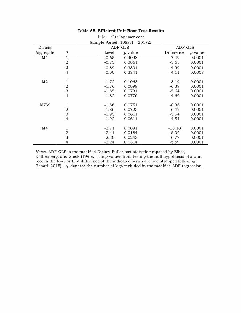
Table A8. Efficient Unit Root Test Results
ln(rt − rta ) : log user cost
Sample Period: 1983:1 – 2017:2 Divisia ADF-GLS ADF-GLS
Aggregate q Level p-value Difference p-value M1 1 -0.65 0.4098 -7.49 0.0001
2 -0.73 0.3861 -5.65 0.0001 3 -0.89 0.3301 -4.99 0.0001 4 -0.90 0.3341 -4.11 0.0003
M2 1 -1.72 0.1063 -8.19 0.0001 2 -1.76 0.0899 -6.39 0.0001 3 -1.85 0.0731 -5.64 0.0001 4 -1.82 0.0776 -4.66 0.0001
MZM 1 -1.86 0.0751 -8.36 0.0001 2 -1.86 0.0725 -6.42 0.0001 3 -1.93 0.0611 -5.54 0.0001 4 -1.92 0.0611 -4.54 0.0001
M4 1 -2.71 0.0091 -10.18 0.0001 2 -2.41 0.0184 -8.02 0.0001 3 -2.30 0.0243 -6.77 0.0001 4 -2.24 0.0314 -5.59 0.0001
Notes: ADF-GLS is the modified Dickey-Fuller test statistic proposed by Elliot, Rothenberg, and Stock (1996). The p-values from testing the null hypothesis of a unit root in the level or first difference of the indicated series are bootstrapped following Benati (2015). q denotes the number of lags included in the modified ADF regression.

Table A9. Efficient Unit Root Test Results
rt − rta : user cost
Sample Period: 1983:1 – 2017:2 Divisia ADF-GLS ADF-GLS
Aggregate q Level p-value Difference p-value M1 1 -0.83 0.3650 -6.59 0.0001
2 -0.89 0.3429 -5.14 0.0001 3 -0.98 0.3105 -4.31 0.0001 4 -1.10 0.2574 -3.94 0.0001
M2 1 -1.94 0.0668 -7.57 0.0001 2 -2.05 0.0473 -5.99 0.0001 3 -2.18 0.0363 -4.97 0.0001 4 -2.37 0.0224 -4.42 0.0001
MZM 1 -2.02 0.0540 -7.83 0.0001 2 -2.05 0.0493 -6.08 0.0001 3 -2.11 0.0410 -4.90 0.0001 4 -2.29 0.0265 -4.19 0.0001
M4 1 -2.73 0.0073 -9.99 0.0001 2 -2.47 0.0188 -8.13 0.0001 3 -2.30 0.0261 -6.56 0.0001 4 -2.35 0.0215 -5.36 0.0001
Notes: ADF-GLS is the modified Dickey-Fuller test statistic proposed by Elliot, Rothenberg, and Stock (1996). The p-values from testing the null hypothesis of a unit root in the level or first difference of the indicated series are bootstrapped following Benati (2015). q denotes the number of lags included in the modified ADF regression.

Table A10. Efficient Unit Root Test Results
vta : consumption velocity
Sample Period: 1983:1 – 2017:2 Divisia ADF-GLS ADF-GLS
Aggregate q Level p-value Difference p-value M1 1 -0.07 0.5419 -4.25 0.0001
2 -0.23 0.5165 -3.84 0.0001 3 -0.28 0.4970 -3.46 0.0005 4 -0.34 0.4889 -3.34 0.0011
M2 1 -0.78 0.4672 -3.36 0.0015 2 -0.78 0.4744 -2.93 0.0049 3 -0.77 0.4852 -2.65 0.0091 4 -0.74 0.4942 -2.24 0.0331
MZM 1 -1.33 0.2081 -4.36 0.0001 2 -1.10 0.2893 -3.87 0.0003 3 -1.14 0.2713 -4.03 0.0001 4 -0.86 0.3787 -3.46 0.0005
M4 1 -0.86 0.3588 -4.20 0.0001 2 -0.86 0.3679 -3.59 0.0004 3 -0.86 0.3642 -3.51 0.0006 4 -0.70 0.3997 -3.02 0.0038
Notes: Consumption velocity is computed by dividing nominal personal consumption expenditures by the indicated monetary aggregate. ADF-GLS is the modified Dickey-Fuller test statistic proposed by Elliot, Rothenberg, and Stock (1996). The p-values from testing the null hypothesis of a unit root in the level or first difference of the indicated series are bootstrapped following Benati (2015). q denotes the number of
lags included in the modified ADF regression.

Table A11. Efficient Unit Root Test Results
ln(mta ) : log money-output ratio
Sample Period: 1983:1 – 2017:2 Divisia ADF-GLS ADF-GLS
Aggregate q Level p-value Difference p-value M1 1 1.00 0.7657 -4.27 0.0001
2 0.91 0.7560 -3.57 0.0007 3 0.64 0.7042 -3.18 0.0017 4 0.52 0.6755 -3.11 0.0026
M2 1 -0.62 0.4923 -2.88 0.0058 2 -0.63 0.4855 -2.67 0.0100 3 -0.54 0.5239 -2.22 0.0322 4 -0.61 0.5067 -2.00 0.0530
MZM 1 -0.89 0.3485 -4.29 0.0001 2 -0.52 0.4578 -3.99 0.0002 3 -0.46 0.4663 -3.64 0.0008 4 -0.44 0.4674 -3.36 0.0011
M4 1 -1.63 0.1288 -3.89 0.0005 2 -1.54 0.1514 -3.32 0.0009 3 -1.55 0.1482 -3.25 0.0015 4 -1.36 0.2024 -2.75 0.0071
Notes: The log money-output ratio is computed by dividing the indicated monetary aggregate by nominal GDP and taking the natural logarithm. ADF-GLS is the modified Dickey-Fuller test statistic proposed by Elliot, Rothenberg, and Stock (1996). The p-values from testing the null hypothesis of a unit root in the level or first difference of the indicated series are bootstrapped following Benati (2015). q denotes the number of
lags included in the modified ADF regression.
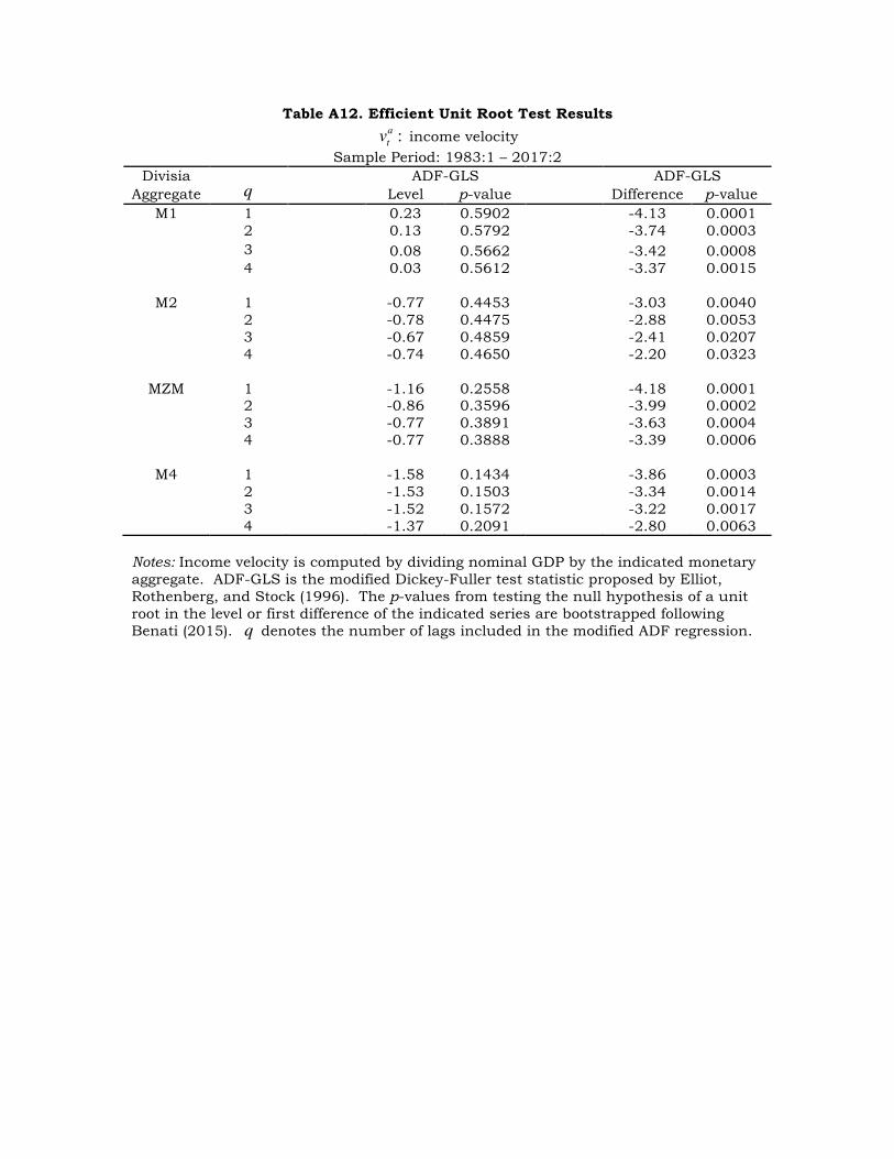
Table A12. Efficient Unit Root Test Results
vta : income velocity
Sample Period: 1983:1 – 2017:2 Divisia ADF-GLS ADF-GLS
Aggregate q Level p-value Difference p-value M1 1 0.23 0.5902 -4.13 0.0001
2 0.13 0.5792 -3.74 0.0003 3 0.08 0.5662 -3.42 0.0008 4 0.03 0.5612 -3.37 0.0015
M2 1 -0.77 0.4453 -3.03 0.0040 2 -0.78 0.4475 -2.88 0.0053 3 -0.67 0.4859 -2.41 0.0207 4 -0.74 0.4650 -2.20 0.0323
MZM 1 -1.16 0.2558 -4.18 0.0001 2 -0.86 0.3596 -3.99 0.0002 3 -0.77 0.3891 -3.63 0.0004 4 -0.77 0.3888 -3.39 0.0006
M4 1 -1.58 0.1434 -3.86 0.0003 2 -1.53 0.1503 -3.34 0.0014 3 -1.52 0.1572 -3.22 0.0017 4 -1.37 0.2091 -2.80 0.0063
Notes: Income velocity is computed by dividing nominal GDP by the indicated monetary aggregate. ADF-GLS is the modified Dickey-Fuller test statistic proposed by Elliot, Rothenberg, and Stock (1996). The p-values from testing the null hypothesis of a unit root in the level or first difference of the indicated series are bootstrapped following Benati (2015). q denotes the number of lags included in the modified ADF regression.

Table A13. Cointegrating Money Demand Relationships
Meltzer Specification: ln(mta ) =α 0 −α1 ln(rt − rt
a ) ln(mt
a ) : log money-output ratio
Sample Period: 1967:1 – 2017:2 Divisia Max Eigenvalue Max Eigenvalue
Aggregate q α 0 α1 r = 0 p-value r = 1 p-value
M1 2*+ -6.69 1.94 44.81 0.0001 3.09 0.6588 3 -7.06 1.98 39.05 0.0001 3.12 0.6658 4 -6.62 1.78 26.80 0.0014 2.51 0.7545 5 -6.33 1.66 21.04 0.0135 2.10 0.8330
M2 2*+ -4.93 1.55 44.20 0.0001 5.53 0.2561 3 -4.98 1.57 43.44 0.0001 5.13 0.3019 4 -5.00 1.58 33.50 0.0001 5.18 0.3038 5 -5.12 1.67 30.70 0.0002 4.13 0.4378
MZM 2*+ -4.70 1.38 39.38 0.0001 5.95 0.2078 3 -4.69 1.37 38.78 0.0001 5.43 0.2591 4 -4.78 1.42 27.95 0.0007 5.57 0.2495 5 -4.78 1.43 26.61 0.0012 4.49 0.3829
M4 2*+ -10.38 5.99 24.13 0.0026 8.62 0.0678 3 -8.79 4.71 21.81 0.0055 8.54 0.0689 4 -35.20 24.83 18.03 0.0309 8.07 0.0888 5 -11.73 6.96 15.37 0.0792 6.81 0.1467
Notes: The log money-output ratio is computed by dividing the indicated monetary aggregate by nominal GDP and taking the natural logarithm. α 0 and α1 are
Johansen's (1991) maximum likelihood estimates of the coefficients of the first
cointegrating vector, normalized so that the coefficient on ln(mta ) equals one. The
maximum eigenvalue test statistics for the null hypothesis of r = 0 and r = 1 cointegrating vectors are shown, together with bootstrapped p-values, computed using the algorithm outlined by Cavaliere, Rahbek, and Taylor (2012). q denotes the number
of lags included in the VAR in levels; the superscripts * and + denote the optimal lag lengths chosen according to the Schwarz (1978) and Hannan-Quinn (1979) criteria.

Table A14. Cointegrating Money Demand Relationships
Cagan Specification: ln(mta ) = δ 0 −δ1(rt − rt
a ) ln(mt
a ) : log money-output ratio
Sample Period: 1967:1 – 2017:2 Divisia Max Eigenvalue Max Eigenvalue
Aggregate q δ 0 δ1 r = 0 p-value r = 1 p-value
M1 2* 0.88 28.02 30.17 0.0007 1.87 0.8501 3+ 2.29 40.01 28.11 0.0007 2.90 0.6723 4 1.12 30.39 17.60 0.0377 2.04 0.8214 5 1.66 34.49 16.51 0.0622 1.65 0.8855
M2 2* -1.32 5.38 41.71 0.0001 5.54 0.2521 3+ -1.16 5.98 42.46 0.0001 5.22 0.2893 4 -1.19 5.92 31.89 0.0005 5.28 0.2881 5 -0.98 6.64 30.55 0.0003 4.33 0.3973
MZM 2 -1.52 4.69 35.13 0.0001 5.94 0.2099 3*+ -1.38 5.24 39.11 0.0001 5.49 0.2681 4 -1.40 5.22 26.22 0.0016 5.54 0.2523 5 -1.29 5.58 26.91 0.0015 4.53 0.3710
M4 2*+ 1.30 13.86 21.39 0.0063 8.66 0.0617 3 0.37 10.74 21.09 0.0099 8.17 0.0819 4 8.52 40.36 16.04 0.0628 8.01 0.0861 5 2.15 17.11 15.30 0.0779 6.65 0.1458
Notes: The log money-output ratio is computed by dividing the indicated monetary aggregate by nominal GDP and taking the natural logarithm. δ 0 and δ1 are
Johansen's (1991) maximum likelihood estimates of the coefficients of the first
cointegrating vector, normalized so that the coefficient on ln(mta ) equals one. The
maximum eigenvalue test statistics for the null hypothesis of r = 0 and r = 1 cointegrating vectors are shown, together with bootstrapped p-values, computed using the algorithm outlined by Cavaliere, Rahbek, and Taylor (2012). q denotes the number
of lags included in the VAR in levels; the superscripts * and + denote the optimal lag lengths chosen according to the Schwarz (1978) and Hannan-Quinn (1979) criteria.

Table A15. Cointegrating Money Demand Relationships
Selden-Latané Specification: vta = γ 0 + γ 1(rt − rt
a ) vta : income velocity
Sample Period: 1967:1 – 2017:2 Divisia Max Eigenvalue Max Eigenvalue
Aggregate q γ 0 γ 1 r = 0 p-value r = 1 p-value
M1 2* -31.40 365.06 26.25 0.0016 2.20 0.7836 3+ -86.89 835.35 24.42 0.0031 3.52 0.5564 4 -40.37 446.39 15.50 0.0747 2.45 0.7453 5 -33.32 381.88 15.72 0.0734 2.01 0.8218
M2 2* -14.01 111.02 33.39 0.0001 3.90 0.4505 3+ -18.64 128.67 33.68 0.0001 3.83 0.4671 4 -19.44 132.49 25.73 0.0021 3.76 0.4901 5 -20.11 133.89 26.28 0.0016 3.24 0.5664
MZM 2 -10.33 98.68 28.68 0.0008 3.97 0.4202 3*+ -15.17 117.60 31.46 0.0002 4.10 0.4376 4 -17.47 127.05 20.90 0.0105 4.02 0.4328 5 -14.41 114.42 22.81 0.0062 3.46 0.5291
M4 2*+ -1678.65 5975.83 20.53 0.0099 6.67 0.1512 3 -354.33 1322.00 19.42 0.0163 6.47 0.1677 4 61.53 -173.20 15.21 0.0822 6.13 0.1900 5 371.27 -1279.26 14.32 0.1134 5.61 0.2322
Notes: Income velocity is computed by dividing nominal GDP by the indicated monetary aggregate. γ 0 and γ 1 are Johansen's (1991) maximum likelihood estimates of the
coefficients of the first cointegrating vector, normalized so that the coefficient on vta
equals one. The maximum eigenvalue test statistics for the null hypothesis of r = 0 and r = 1 cointegrating vectors are shown, together with bootstrapped p-values, computed using the algorithm outlined by Cavaliere, Rahbek, and Taylor (2012). q
denotes the number of lags included in the VAR in levels; the superscripts * and + denote the optimal lag lengths chosen according to the Schwarz (1978) and Hannan-Quinn (1979) criteria.
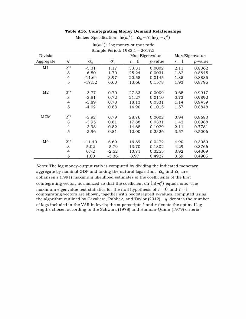
Table A16. Cointegrating Money Demand Relationships
Meltzer Specification: ln(mta ) =α 0 −α1 ln(rt − rt
a ) ln(mt
a ) : log money-output ratio
Sample Period: 1983:1 – 2017:2 Divisia Max Eigenvalue Max Eigenvalue
Aggregate q α 0 α1 r = 0 p-value r = 1 p-value
M1 2*+ -5.31 1.17 33.31 0.0002 2.11 0.8362 3 -6.50 1.70 25.24 0.0031 1.82 0.8845 4 -11.64 3.97 20.58 0.0145 1.85 0.8885 5 -17.52 6.60 13.66 0.1578 1.93 0.8795
M2 2*+ -3.77 0.70 27.33 0.0009 0.65 0.9917 3 -3.81 0.72 21.27 0.0110 0.73 0.9892 4 -3.89 0.78 18.13 0.0331 1.14 0.9459 5 -4.02 0.88 14.90 0.1015 1.57 0.8848
MZM 2*+ -3.92 0.79 28.76 0.0002 0.94 0.9680 3 -3.95 0.81 17.88 0.0331 1.42 0.8988 4 -3.98 0.82 14.68 0.1029 2.11 0.7781 5 -3.96 0.81 12.00 0.2326 3.57 0.5006
M4 2*+ -11.40 6.69 16.89 0.0472 4.90 0.3059 3 5.02 -5.79 13.70 0.1302 4.29 0.3766 4 0.72 -2.52 10.71 0.3255 3.92 0.4309 5 1.80 -3.36 8.97 0.4927 3.59 0.4905
Notes: The log money-output ratio is computed by dividing the indicated monetary aggregate by nominal GDP and taking the natural logarithm. α 0 and α1 are
Johansen's (1991) maximum likelihood estimates of the coefficients of the first
cointegrating vector, normalized so that the coefficient on ln(mta ) equals one. The
maximum eigenvalue test statistics for the null hypothesis of r = 0 and r = 1 cointegrating vectors are shown, together with bootstrapped p-values, computed using the algorithm outlined by Cavaliere, Rahbek, and Taylor (2012). q denotes the number
of lags included in the VAR in levels; the superscripts * and + denote the optimal lag lengths chosen according to the Schwarz (1978) and Hannan-Quinn (1979) criteria.

Table A17. Cointegrating Money Demand Relationships
Cagan Specification: ln(mta ) = δ 0 −δ1(rt − rt
a ) ln(mt
a ) : log money-output ratio
Sample Period: 1983:1 – 2017:2 Divisia Max Eigenvalue Max Eigenvalue
Aggregate q δ 0 δ1 r = 0 p-value r = 1 p-value
M1 2*+ 0.21 25.26 32.17 0.0001 1.67 0.8969 3 3.15 51.72 27.28 0.0015 2.28 0.8082 4 -9.86 -64.23 22.27 0.0067 2.29 0.8081 5 -6.32 -32.60 16.89 0.0576 3.03 0.6884
M2 2*+ -1.90 3.38 24.92 0.0027 0.62 0.9926 3 -1.92 3.31 19.32 0.0218 0.77 0.9811 4 -1.83 3.61 17.49 0.0399 1.42 0.8995 5 -1.86 3.51 16.07 0.0721 2.09 0.7839
MZM 2*+ -1.83 3.81 26.48 0.0014 0.94 0.9703 3 -1.81 3.87 17.88 0.0303 1.42 0.8977 4 -1.77 4.01 15.61 0.0775 2.26 0.7420 5 -1.90 3.58 13.64 0.1556 3.90 0.4392
M4 2*+ -21.71 -68.87 16.35 0.0500 5.02 0.2871 3 -5.95 -12.10 13.73 0.1310 4.32 0.3828 4 -4.29 -6.08 10.57 0.3302 3.94 0.4279 5 -4.84 -8.01 9.91 0.3959 3.42 0.5171
Notes: The log money-output ratio is computed by dividing the indicated monetary aggregate by nominal GDP and taking the natural logarithm. δ 0 and δ1 are
Johansen's (1991) maximum likelihood estimates of the coefficients of the first
cointegrating vector, normalized so that the coefficient on ln(mta ) equals one. The
maximum eigenvalue test statistics for the null hypothesis of r = 0 and r = 1 cointegrating vectors are shown, together with bootstrapped p-values, computed using the algorithm outlined by Cavaliere, Rahbek, and Taylor (2012). q denotes the number
of lags included in the VAR in levels; the superscripts * and + denote the optimal lag lengths chosen according to the Schwarz (1978) and Hannan-Quinn (1979) criteria.

Table A18. Cointegrating Money Demand Relationships
Selden-Latané Specification: vta = γ 0 + γ 1(rt − rt
a ) vta : income velocity
Sample Period: 1983:1 – 2017:2 Divisia Max Eigenvalue Max Eigenvalue
Aggregate q γ 0 γ 1 r = 0 p-value r = 1 p-value
M1 2*+ -0.24 125.92 30.00 0.0005 1.88 0.8570 3 -2.16 144.55 23.46 0.0043 1.88 0.8559 4 -9.62 209.91 19.09 0.0275 1.74 0.8738 5 -14.99 256.83 15.04 0.1024 2.22 0.8114
M2 2*+ 4.02 47.26 25.06 0.0027 0.57 0.9951 3 4.31 46.39 19.22 0.0222 0.56 0.9957 4 3.49 49.25 17.23 0.0467 0.83 0.9759 5 3.67 48.74 15.67 0.0819 1.21 0.9310
MZM 2*+ 2.40 55.88 26.20 0.0020 0.88 0.9708 3 2.35 56.50 17.79 0.0355 1.04 0.9564 4 1.88 58.23 15.10 0.0936 1.50 0.8892 5 3.27 53.37 12.96 0.1799 2.31 0.7296
M4 2*+ -165.74 645.98 16.50 0.0483 4.54 0.3363 3 74.67 -220.70 14.00 0.1215 4.07 0.4105 4 41.13 -99.68 10.68 0.3194 3.70 0.4700 5 44.73 -111.66 9.88 0.3996 3.30 0.5354
Notes: Income velocity is computed by dividing nominal GDP by the indicated monetary aggregate. γ 0 and γ 1 are Johansen's (1991) maximum likelihood estimates of the
coefficients of the first cointegrating vector, normalized so that the coefficient on vta
equals one. The maximum eigenvalue test statistics for the null hypothesis of r = 0 and r = 1 cointegrating vectors are shown, together with bootstrapped p-values, computed using the algorithm outlined by Cavaliere, Rahbek, and Taylor (2012). q
denotes the number of lags included in the VAR in levels; the superscripts * and + denote the optimal lag lengths chosen according to the Schwarz (1978) and Hannan-Quinn (1979) criteria.

Figure A1. Divisia Monetary Data. The log money-output ratio in column one and income velocity in column two are computed using nominal GDP as the scale variable.

Figure A2. Divisia Money Demand Relationships. Each scatterplot compares the indicated Divisia monetary aggregate, scaled by nominal GDP, measured along the vertical axis, to the associated user cost aggregate, measured along the horizontal axis. The Meltzer (1963) specification relates the log money-output ratio to the log of the user cost; the Cagan (1956) specification relates the log money-output ratio to the level of the user cost; the Selden-Latané specification relates the income velocity of money to the level of the user cost.