the demand for electricity: a cross-section study of new south wales and the australian capital...

The Demand for Electricity: A Cross- section Study of New South Wales and the Australian Capital Territory*

Economists have long argued that electricity prices should reflect marginal costs. Although the debate has revolved mainly around the question of time-of-day pricing,l another important cause of distortion is the imposition of uniform tariffs across a wide geographical area.2 In either case, the size of possible allocative distortions depends crucially on the sensitivity of demand to changes in electricity prices. There are, however, no published Australian studies investigating t h i s relationship.

More generally, the current supply upheavals in the energy market have cast doubt on the accuracy of forecasts of future energy demand that do not explicitly consider the effects of energy prices on the demand for fuels. Unfortunately, few reliable estimates of demand elasticities are available, and there are none explicitly for Australia,

This paper investigates an important component of the demand for energy, namely the demand for electricity, at retail level, by residential, commercial and industrial consumers. The principal objective is to determine the effects on total demand for electricity of variations in electricity prices. Also considered are the effects of competition from gas and other fuels, and the importance of economic determinants such as household income and the level of commercial activity. Multiple regression techniques are employed on a cross-section of data for electricity retailing authorities in New South Wales and the Australian Capital Territory. The choice of data enables an explicit representation of the supply side of the electricity market to be achieved. Consistent estimation of the demand equations then provides estimates of demand elasticities, unbiased by supply-side effects.

Section 1 contains a brief description of the organization of the electricity market in New South Wales and its place in the overall

*The author is grateful for the comments of R. G. Gregory, A. R. Pagan, an anonymous referee, and the participants in seminars at the Australian National T Jniversity. Any remaining errors are solely his own responsibility. An earlier version of this study was issued as a working paper [14].

1 Australian contributions to the debate include Kolsen [17] and Harvey [13]. 2 State-wide uniform electricity tariffs were introduced in Victoria in 1965.

Harvey [13] suggests that this represents an annual subsidy of a t Ieast $3 m. to rural consumers. The pressure for the introduction of uniform taritfs in New South Wales remains strong, as is evidenced by the Report of the Retail Tariffs Committee of the Local Government Electricity Association [ 181.

1 A

MARCH 2 THE ECONOMIC RECORD

energy market. Section 2 formulates theoretical models, which are then estimated in Section 3. The final section draws the results together and explores some of their implications.

1. Retail Electricity Markets in New South Wales and the Australian Capital Territory

Kalma et al. [16] have made a general survey of energy flows in New South Wales in the year 1970. They estimate that industry ac- counted for about 59 per cent of energy use, transportation for 29 per cent, and the commercial and domestic sectors each for 6 per cent.

In the industrial sector black coal is the dominant fuel, providing 69 per cent of the energy input,3 compared with petroleum fuels’ 23 per cent and electricity’s mere 7 per cent. In the commercial sector petroleum products account for 56 per cent of energy use and electricity for 28 per cent. In the domestic sector electricity is the principal source of energy, with 58 per cent, while reticulated gas and petroleum products each provide about 16 per cent. Of the electricity consumption 44 per cent takes place in the industrial sector, 14 per cent in the commercial sector and 38 per cent in the domestic sector.

In 1971, over 80 per cent of the electricity consumed was sold by 44 retail a~thorities.~ Of these 34 were county councils, 5 were city, municipal or shire councils and.5 were franchise holders. The Australian Capital Territory was served by its own authority. There was a wide dispersion of authority sizes. At one extreme was Sydney County Council, with 565,000 residential customers; at the other, lvanhoe franchise with 95 customers. There were wide variations in the proportions of residential, commercial and industrial customers, and in the degree of urbanization and population den~ity.~

The Australian Capital Territory draws the bulk of its electricity from the Snowy Mountains Authorit? and the remainder from the Electricity Commission of New South Wales. In New South Wales all the eouncils draw at least part of their supplies from the Electricity Commission. The franchise holders generate the whole of their requirements, and some of the councils a part of their requirements. The Electricity Commission charges all councils according to a single schedule of charges, irrespective of location. The schedule is in two parts: a constant energy charge per kilowatt hour (kwh) and a maximum demand charge per kilowatt (kw), drawn during the daily period of

9 These percentages exclude fuel used in electricity generation, gas manufacture and oil refining, but include material inputs, for example to coke works. All energy flows are measured as gross calorific values.

.I The remainder of the electricity was sold in bulk by the Electricity Commis- sion of New South Wales and other authorities.

For further analysis of Australian electricity markets, see Harvey [13], f(olsen [17], McColl [20] and Prest [Z].

6The proportion was 82.5 per cent in 1971-72.

1975 DEMAND FOR ELECTRICITY 3 potential peak demand.7 l’he maximum demand meters are reset monthly, and the demand charge is revised quarterly in line with wage and material costs.

Average demand per customer is highest in the industrial sector, where it varies between authorities from 30,000 to 9,000,OOO kwh per annum. In the commercial sector it varies from 6,000 to 40,000 kwh per annum and in the residential sector from 1,OOO to 7,000. Average receipts per kwh range from 1.5 to 7.2 cents for residential sales, from 1.9 to 7.9 cents for commercial sales and from 1.3 to 6 .9 for industrial sales. However, the upper limits are reduced to 3.1, 4 . 0 and 3 1 cents per kwh if the two smallest franchises are excluded. There is a similar degree of variation in marginal electricity prices.

2 . Models of Electricity Demand Three distinct models are developed in this section. The first

explains the demand for electricity by residential customers. The second is designed to test the responsiveness of commercial and industrial demand to variations in the price of electricity. The third explores the relationships between commercial and industrial activity, employment and the consumption of electricity.

(a) Residential Demand Residential demand for electricity is represented by a two-equation

system explaining average consumption per electricity customer and the proportion of electricity customers with a gas connection.

As with other consumer goods, demand for electricity should depend on a consumer’s real income, tastes, and the relative prices of electricity and substitute fuels. However, the demand for an energy material, such as electricity, differs in two important respects from the demand for other non-durable consumer goods. First, electricity is desired, not for its own sake, but because it enables a flow of services to be obtained from existing consumer durables. Secondly, the provision of a supply of a particular fuel to a consumer may require a considerable capital investment.

As regards the first point, the stock of electrical appliances is more or less fixed in the short run. If, as seems likely, utilization rates of existing appliances are insensitive to changes in electricity prices, then the demand for electricity should be price and income inelastic in the short run.* In the longer run, the stock of appliances can be varied and the consumer’s choice of fuel for a particular application will depend

7 I t is this uniformity of price schedules at the wholesale level that makes it possible to model the retail supply side of the market explicitly and hence to obtain consistent estimates of parameters in the demand equations. For further details, see [14]. It should be noted that the uniform wholesale tariff schedule is itself a potential contributor to allocative distortions ; but that is outside the scope of this paper.

8 Fisher and Kaysen [ l l ] is the only study to attempt to test this assertion. They suggest that demand is significantly affected by price changes in the short run. Later American studies, for example [24], discount their results.

4 THE ECONOMIC RECORD MARCH

on the prices and efficiencies of the different appliances, as well as on the prices of the various fuels.

The dependence of electricity demand on the prices and efficiencies of appliances has proved a considerable stumbling-block to time-series analysis of residential electricity demand.O Fortunately, the prices of many appliances are high relative to possible variations due to transport costs. In a cross-sectional study, it therefore seems reasonable to assume that the prices of appliances are constant and that their technology is everywhere the same.1° The results of such a study should provide a clear indication of the partial effects, on the demand for electricity, of variations in the prices of fuels, but only within a given framework of appliance prices and technology.ll

There is the further point that the provision of a particular fuel to a consumer may require a considerable capital investment. In some areas particular energy types are unavailable, and in others the consumer may have to pay heavily to acquire a supply.12 Consumers may therefore be. expected to behave differently, depending on whether they have connections to particular fuel supplies. This suggests that households should be grouped according to the fuel supplies available in their areas, and according to their access to particular fuels. In this study attention is confined to households possessing an electricity connection. These are divided into two groups, those with and those without a gas supply.*3 The behaviour of each of these groups is considered in turn.

For households with a gas connection, the average demand for

BSee especially Fisher and Kaysen [ l l ] , and Wilson’s [25] comments on their study. The main problem is the lack of reliable data for appliance stocks and prices, and for the consumption of electricity in each type of appliance. Where the problem is ignored, as by Wigley [24], the estimated price and income elasticities may be biased.

10 Any tendency for manufacturers and chain stores to impose uniform retail prices would help to support this assumption.

11 An additional problem, introduced by the dependence of electricity consumption on appliance stocks, is that the current levels of stocks, and hence of electricity consumption, may differ from their long-run equilibrium levels. Anderson [2] has tried to adapt a stock-adjustment model for use with cross- sectional data from successive years. But he does not tackle the possibly formidable effects of autocorrelation on the estimated coefficients. It seems preferable, at least initially, to choose a data sample from a stable market, in which the disequilibrium effects should be small. I t is suggested that the New South Wales market in 1971 satisfies this requirement.

12This is particularly so in the case of electricity and reticulated gas and in country areas. Reticulated gas is available only in certain urban areas, and rural consumers pay a portion of the considerable costs of providing electricity connections. For example, the Australian Financial Review (10 January 1974) mentions instances of rural electricity connections costing developers and house- holders between $1,000 and $1,800.

13 In the earlier version of this study [ 131, equations were estimated to explain the proportions of households with and without electricity connections. The variation in this proportion is extremely small and the equations are therefore omitted from this paper. Considerable effort was also devoted during initial experiments to distinguishing between the behaviour of households with bottled gas (1.p.g.) and reticulated gas connections, but to little effect. The theoretical model is easily extended to this more general case.

1975 DEMAND FOR ELECTRICITY 5 electricity14 (De,) should depend on household average real income ( Y ) , geographical and demographic factors (X) and the deflated prices of electricity ( P e ) , gas ( P , ) and other fuels such as heating oil (Po).15 Assuming a linear demand function, this may be written as:

(1) For households without a gas connection, the price of gas does not

(2) The available data for electricity consumption aggregate these two

categories. Therefore, supposing that Ne, households have electricity and gas connections and N,, have only electricity, such that N e = Ne, + Neo, the average household electricity demand ( D , ) is given by:

Deg = ao + + a d + ad’e + a4P0 + USP,.

enter the average demand function. Thus:

Deo = bo + b1Y + bzX + bsPe + b 8 o .

De = (DepNeg + Deo*Neo)/Ne. ( 3 )

Substitution from equations (1) and (2) into (3 ) gives:

De = (aoNeg +boNeo)INe +(alNeg+hNeJ Y/Ne +(a,Neg+b,Neo)X/Ne +(a8eg +baNeo)Pe/Ne +(aJVeg +baNeo)Po/Ne fasNep Pg/Ne. (4)

This is the equation used in estimation. Obviously (4) can be s u b stantially simplified if a number of corresponding 6 and b4 can be shown empirically to be identical.

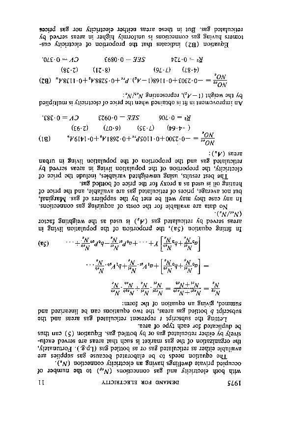
Equations are now derived for the proportion of households having both gas and electricity connections. In any area, the proportion of residential electricity customers having a gas connection depends on the gas supplies available, on the costs of acquiring a connection, and on the household‘s real income, tastes and the prices of other fuels. This proportion may be written:

( 5 ) where V is some index of the availability of supply and 2 is the cost to households of a gas connection. In practice a linear approximation of this function is used.

(b) Commercial and Industrial Demand The scanty evidence available from time-series studies [21], [24]

suggests that commercial electricity consumption is price inelastic but 1 4 Use of average demand as the dependent variable is necessary because the

data for individual households do not exist. It also helps to alleviate the heteroskedasticity that would be introduced into the estimation by the use of total demand as the dependent variable. The problem of heteroskedacity is further considered below.

‘“or some fuels, such as electricity, stepped tariffs apply. The average and marginal prices paid by the consumer differ in these cases. The question of choosing appropriate price variables is further considered below.

Neq/Ne = Ncg( Vm zo Y , X, P o Pg, Po)


varies with the level of commercial activity and with time.le Industrial demand for electricity has not received particularly extensive study either. Time-series studies [ 5 ] , [24] find little evidence of elastic response to electricity price changes, but are bedevilled by multicollinearity. Cross-section studies [ 11 do find evidence of responsiveness to variations in the electricity price, but the estimates may suffer from bias caused by the influence of energy prices on industrial location.

Two models are advanced to explain commercial and industrial electricity consumption. The first supposes that demand for electricity ( E ) by a particular industry group is determined by cost minimization, subject to a production function, to prices of factors, including electricity (Pk, PL, P , ) and to an output target (Z) :

In the second approach the industry’s production function is solved directly for electricity consumption:

E = g(z , Pk, P L Y pe l - (6)

E = h(2, K, L). (7) In both equations, K , L represent capital and labour respectively.

These equations are estimated below.

3. Empirical Results In this section empirical results are presented in turn for each of

the estimated equations. Before proceeding to a d-iled discussion it is appropriate to consider the choice of estimation technique.

The system of equations to be estimated is linear in parameters within each equation, but non-linear in variables.17 It is essential to ensure that consistent parameter estimates are obtained, but a maximum likelihood method is too laborious. Instead, instruments are constructed for each of the endogenous variables by the method of non-linear two- stage least squares, described in Goldfeld and Quandt [12]. These instruments are substituted for the corresponding endogenous variables, whenever they appear as arguments in an equation, thus ensuring consistent estimates.

A further estimation problem is caused by the likelihood of heteroskedasticity in the demand equations.’* Total demand in each category is the sum of the purchasing decisions of all consumers. If consumers’ decisions are statistically independent, then the residuals in an equation

18 There have been very few published studies of commercial electricity demand, though it is an increasingly important energy-consuming sector. The main reason for the lack of interest appears to be the poor quality of the data generally available.

17The complete system includes equations for electricity prices and is described in [ 141. The non-linearities are introduced through the price equations.

1 s I t is also possible that the residuals of different estimated equations are correlated. This possibility is judged most likely to affect the equations for residential and commercial electricity prices. However, use of an Aitken estimator on the ordinary least squares versions of these equations does not cause any appreciable changes in coefficients or t-statistics. Therefore the possiblity is ignored.

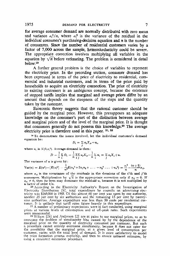
1975 DEMAND FOR ELECTRICITY 7 for average consumer demand are normally distributed with zero mean and variance ui2/n, where U? is the variance of the residual in the individual consumer’s purchasing4ecision equation and n is the number of consumers. Since the number of residential customers varies by a factor of 7,000 across the sample, heteroskedasticity could be severe. The appropriate correction involves multiplying all variables in the equation by VTbefore estimating. The problem is considered in detail below.lB

A further general problem is the choice of variables to represent the electricity price. In the preceding section, consumer demand has been expressed in terms of the price of electricity to residential, commercial and industrial customers, and in terms of the price paid by households to acquire an electricity connection. The price of electricity to existing customers is an ambiguous concept, because the existence of stepped tariffs implies that marginal and average prices differ by an amount that depends on the steepness of the steps and the quantity taken by the customer.

Economic theory suggests that the rational customer should be guided by the marginal price. However, t h i s presupposes an adequate knowledge on the consumer’s part of the distinction between average and marginal prices and of the level of the marginal price. It is thought that consumers generally do not possess this knowledge.20 The average electricity price is therefore used in this paper. 21. 2a

‘9 To demonJtrate the issues involved, let the individual customer’s demand equation be :

D; = aJj,+ui, 3

where u, is ,V(O,utn). Average demand is then: 1 1 1

“ i “ i j “ i i D = - 2: D; = - C C a j 9 , ; f - C U, = C ajX,+u.

The variance of u is given by :

Var(u) = ~ ( u ? ) - [ [ E ( u ) ? ] = -E(u,2+Ou1uII+ . . . +u,?. . . +un2) = l+-

where us, is the covariance of the residuals in the decisions of the i’ th and j’th consumers. Multiplication by & is the appropriate correction only if u,! = 0. If uf, # 0, then its term may dominate the residual u, because i t is not multiplied by a factor of order l jn.

20 According to the Electricity Authority’s Report on the Investigation of Electricity Distribution [9], total expenditure by councils on advertising electricity was $560,000 in 1965. Of this almost 60 per cent was spent by one authority, another 25 per cent by six authorities and the remaining 15 per cent by twenty- nine authorities. Average expenditure was less than 50 cents per residential customer. It is unlikely that tariff rates figure heavily in this expenditure.

21 A number of preliminary experiments were in fact conducted, using marginal prices at various levels of consumption and at off-peak rates. Such experiments

1 u 2 h+ l)u,f, na n n

were unsuccessful. “\Vilson [21] and Anderson [ 2 ] are at pains to use marginal prices, so as to

overcome the prohlem of simultaneity bias caused by by the dependence of the marginal price on the quantity of electricity consumed per customer. But such a procedure cannot entirely overcome simultaneity. because it does not cater for the possibility that the marginal price, a t a given level of consumption per customer, varies with the total level of demand. I t is more satisfactory to model the price formation process explicitly, and then to ensure unbiased estimates, by using a consistent estimation procedure.


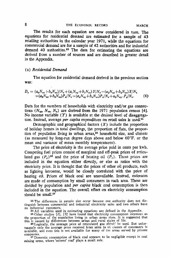
The results for each equation are now considered in turn. The equations for residential demand are estimated for a sample of 43 retailing ,authorities in the calendar year 1971, while the equations for commercial demand are for a sample of 42 authoritia and for industrial demand 40 auth~ri t ies .~~ The data for estimating the equations are derived from a number of sources and are described in greater detail in the Appendix.

(a) Residential Demand

The equation for residential demand derived in the previous section was :

Data for the numbers of households with electricity and/or gas C O M ~ C - tions ( N e g , N,,, N,) are derived from the 1971 population census [4]. No income variable (Y) is available at the desired level of disaggrega- tion. Instead, average per capita expenditure on retail sales is used.24

Demographic and geographical factors (X) include the proportion of holiday homes in total dwellings, the proportion of flats, the proportion of population living in urban areas,25 household size, and climate (as measured by long-run degree days above and below 60°F. or the mean and variance of mean monthly temperatures).

The price of electricity is the average price paid in cents per kwh. Competing fuel prices consist of marginal and off-peak prices of reticulated gas and the price of heating oil ( P o ) . These prices are included in the equation either directly, or else as ratios with the electricity price. It is thought that the prices of other oil products, such as lighting kerosene, would be closely correlated with the price of heating oil. Prices of black coal are unavailable. Instead, estimates are made of consumption by small consumers in each area. These are divided by population and per capita black coal consumption is then included in the equation. The overall effect on electricity consumption should be small.27

23The differences in sample size occur because one authority does not dis- tinguish between commercial and industrial electricity sales and two others have no industrial customers.

24 All variables used in estimating equations are defined in the Appendix. 25 Other studies [2], [3] have found that electricity consumption increases as

the proportion of the population living in urban areas rises, I t is suggested that this is caused by differences between urban and rural styles of life.

2eLogically, the average price of reticulated gas shoul:l be used. But unfortunately only the average price received from sales to a l l ciasses of consumers is available, and even this is not available for many of the areas served by private companies.

27 Domestic consumption of black coal appears to be negligible except in coal mining areas, where 'miners' coal' plays a small role.

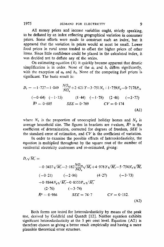
1975 DEMAND FOR ELECTRICITY 9 All money prices and income variables ought, strictly speaking,

to be deflated by an index reflecting geographical variation in consumer prices. Some efforts were made to construct such an index, but it appeared that the variation in prices would at most be small. Lower food prices in rural areas tended to offset the higher prices of other items. Since little confidence could be placed in the calculated index, it was decided not to deflate any of the series.

On estimating equation ( 4 ) it quickly became apparent that drastic simplification is in order. None of the a, and b4 differs significantly, with the exception of a. and bo. None of the competing fuel prices is significant. The basic result is:

NOeg --+2*621 Y-3.751N,+l *759NP-0*7178P,, NOe

D, = -1.727-1.049

(-0.64) (-1.15) (1.44) (-1.78) (2.46) (-3.77) R2 = 0.605 SEE = 0.769 CV = 0.174

(All

where N h is the proportion of unoccupied holiday homes and N , is average household size. The figures in brackets are t-values, Kz is the coefficient of determination, corrected for degrees of freedom, SEE is the standard error of estimation, and CV is the coefficient of variation.

In order to examine the possible effects of heteroskedasticity, the equation is multiplied throughout by the square root of the number of residential electricity customers and re-estimated, giving:

(-0.21) ( - 2 * 96) (4.27) (-3.73)

+ 0.8 844 N , 4 x- 0 * 8 5 5 3 P, 4

R2 = 0.986 SEE = 74.7 cv= 0.112. (2 * 76) (-3.74)

(A21

Both forms are tested for heteroskedasticity by means of the peak test, derived by Goldfeld and Quandt [ 121. Neither equation exhibits significant heteroskedasticity at the 5 per cent level. Equation (A2) is therefore chosen as giving a better result empirically and having a more plausible theoretical error structure.


The only other determinant to effect a possible improvement in equation (A2) is per capita black coal consumption ( B ) . Addition of this variable gives:

D,1/M, =

(0.26) (-3.45) (3 .77) (-3.73)

(3.13) (- 4 *47) (- 1 -93) +O * 9 125Nfl-0 * 9325P,,dK-2 * 3 7 6 B d z

R2 = 0.988 SEE = 69.3 CV = 0.104.

643) On the basis of equation (A3) the estimated price and expenditure

elasticities of domestic electricity demand, calculated at the sample means, are -0.554 and 0.926 respectively. The elasticity is 0.699 for average household size, -0.0416 for the proportion of holiday homes, -0 126 for the proportion of electricity customers having a gas connection, and -0,0175 for black coal consumption. These results are of the expected sign and all are of reasonable magnitude. Domestic electricity demand responds significantly but inelastically to price and income and declines as the number of gas connections and holiday homes increases. It may be thought strange that black coal consumption should show some effect, where the price of heating oil does not. Possibly the explanation lies in some difference in tastes between coal mining and other areas.

Among the points to be gleaned from equation (A3), the Austra- lian Capital Territory's present high electricity consumption would, it appears, be reduced by 800 kwh a year per household if the proportion of households with a gas connection was as high as in Sydney, and by 1,000 kwh a year if the price rose to the sample average. A coastal area such as Bega Valley would increase its average annual consumption by 1 , 1 0 0 kwh if the proportion of holiday homes fell to the sample average.

The independence of electricity consumption from long-run climatic conditions is rather surprising. Addition of climatic variables to ( A l ) or (A2) suggests that electricity consumption is lower along the coast than inland, but not significantly.

(b) Number of Residential Gas Customers This equation is based on (5 ) :

N, , /N , = NeAVg, z,, y, x, pop,, P o ) . ( 5 ) The dependent variable is derived from the 1971 population census and consists of the ratio of the number of occupied private dwellings


&ect the number of connections. Presumably the number of connections is historically given, In bottled gas areas, the number of gas connections is strongly influenced by the electricity price, but there is no effect of other fuel prices, possibly because the data are poor or because variation in electricity prices is much greater than .variation in gas prices.

There is no evidence of heteroskedasticity in these equations.

(c) Commercial and Zndustrial Demand

In the previous section two equations were suggested to explain commercial and industry electricity consumption. Equation ( 6 ) relates electricity consumption to the level of activity and factor prices:

Equation (7) relates electricity consumption to output and the inputs of capital and labour:

(7 1 Linearized forms of equations are estimated for each of the categories, commercial and industrial electricity consumption.

The measure of electricity demand used is average consumption per commercial ( D p ) or industrial (0 , ) customer. The measures of commercial and industrial activity (2 ) available are generally rather inadequate. The activity variables used are, in the commercial sector, average retail sales per electricity customer ( S / M , ) and the average number of commercial employees other than in retailing ( J J M , ) . In the industrial sector, only employment variables are available, namely the average number of employees in manufacturing (lm/M4), mining and quarrying (]*/Mi), and electricity, gas and water ( J e / M i ) . These variables are taken from the 1971 population census [4] and from the Census of Retail Establishments [ 5 ] . It might be thought that the new integrated economic census would provide useful variables. However, the data for manufacturing industry are available only for Statistical Divisions, which are too aggregated for the purpose of this study.

The user costs of capital (Pk) and labour (PI,) appear in equation (6). The user cost of capital is a complicated expression involving the price of capital goods, interest and depreciation rates, and taxation variables. Since it is unlikely that many of these vary geographically, and they are in any case unobtaiiable, the user cost of capital is omitted. The user cost of labour ( P L ) is approximated by the average earnings per retail employee, drawn from the integrated economic census. Also included are the average price of electricity, the price of the heating oil and the marginal price of reticulated gas, together with the per capita consumption of black coal.

Lastly, a dummy variable ( F 1 ) is included in the equation for commercial consumption in the case of the Australian Capital Territory,

E = h ( Z , K, L ) .

1975 DEMAND FOR ELECTRICITY 13 because the number of commercial enterprises is controlled, particularly the number of small retail establishments. The average electricity consumption is therefore expected to be exceptionally high in the Australian Capital Territory.

Equation ( 6 ) is then estimated for commercial and industrial electricity demands. The preferred results are given below.

Commercial demand

Dc = -7 ~292 +22'62F, +O '0907(S/Mc) + 1 * 358(Jc/Mc)- I * 126P,, ( -1 '27) (4.81) (0.74) (2.11) (-2.14) + 1 1 *35PL

(2-69)

= 0.832 SEE = 3.03 CV = 0,237.

D, = 6.5 5 3 +28.9 3 Fl +O *23 19( S / M , ) +- 1 * 1 36(J,/M,) -0 -68 13 P,,

(2.41) (6.56) (1 *94) (1.64) (-1.26) R2 = 0.804 SEE = 3.27 CV = 0.256

Industrial demand

Di = 9.390+9.831{ ( J , + I , + J , ) / M { } -33.22P,,

(0.02) (12.96) (-0.2 1)

R2 = 0.832 SEE = 750.0 CV = 0.71 1 .

Equation (D1 ) suggests that commercial demand for electricity is sensitive to the price of electricity and to the wage rate. This finding is at variance with those of other studies [20], [23]; the elasticity of electricity consumption with respect to changes in the wage rate is suspiciously high at 1.4, and it is surprising to find that retail sales have a low, insignificant coefficient. I t is possible that high retail wages are associated with high levels of sales per retailer. Therefore the equation is also estimated without the retail wage.

Equation (D2) provides a more accepta'ble coefficient on the retail sales variable. As in the equation for industrial demand (D3) , the electricity price is insignificant. This equation is therefore preferred.

(d) Output, Employment and Electricity Consumption An alternative explanation of commercial and industrial electricity

consumption was derived in the previous section by solving the production function for electricity consumption. Thus:

Equation (7) is estimated in log-linear form. E = h ( Z , K , L ) . (7)


The variables used are the same as those employed in the estimation of equation (6) , with some exceptions. All price variables are omitted, and the average number of retail employees per commercial customer ( I J M , ) is added to the equation for commercial electricity demand. The preferred results are as follows.

Commercial demand

Ln D , = -0.8666+0*3802+0.7873 Ln(S/Mc)-l.031 Ln(J,/M,)

(-1.25) (1.16) (3.32) (-3 * 12) +O a986 1 Ln(J, + Jc/Mc) (El)

(3.54) R2 = 0.705 SEE = 0.222 CV = 0.091.

Industrial demand

Ln D , = 2.715+0 8491 Ln{ (J , , ,+JQ+Je) /ML} (E2 1 (9-76) (12.44)

Ra = 0.798 SEE = 0.662 cv = 0.1 12.

It is diflicult to interpret the industrial result, since no activity variable is included in the equation. If the employment variable were taken as a proxy for the activity level (Y), then the equation would suggest that there were increasing returns to scale in industrial electricity consumption, Y = A DZ1.l8. But any such interpretation must be very tentative.

The commercial result shows that electricity demand varies positively with average retail sales and negatively with the average number of retail employees. The production function for retailing implied by these estimates is approximately:28

S/Mr = A F l a . ( D J M , ) '."O. (Jr /M,) .057

where M , is the number of commercial electricity customers engaged in retailing. Since the sum of the exponents (1.33) is greater than one, this function exhibits increasing returns to scale. It also has a very low labour exponent.

It would be interesting to compare this production function with estimates from other studies. However, there is a surprising dearth of production function estimates for retailing. The few studies surveyed by Walters [23] do provide some evidence of increasing returns to scale. But more recent studies, such as [19], have questioned such findings, on the ground that theTe is considerable heterogeneity in the data samples

as opposed to log-linear, production function. 2aThe production function is exactly recoverable only in the case of a linear,

1975 DEMAND FOR ELECTRICITY 15

of most cross-section studies, and that the derived estimates of eco- nomies of scale are thus meaningless.

Such arguments should arouse scepticism in evaluating the results presented here. However, most of the areas in the sample are either large in population or else distant from other retailing centres. The sample of commercial enterprises may therefore be reasonably homo- geneous in composition. Perhaps a more serious objection is that the activity variable is the value of sales. It could be that a high level of electricity consumption in retailing implies a high level of selling effort, which allows a high mark-up to be charged. Therefore retail sales could overstate activity in areas with high retail sales. This would bias downwards the estimated coefficient on the activity variable and hence provide an overestimate of returns to scale.

4. Conclusions

The experiments described in this paper throw some light on the main determinants of retail demand for electricity in Australia.

Residential electricity has been shown to be a marginally inferior good which is moderately price inelastic. It is positively related to household size and negatively to the proportion of holiday homes. Climatic variables and the prices of most competitive fuels do not appear to influence the demand for electricity." The number of households having a gas connection does influence demand, but there is no additional influence of gas prices.

The study also explains the proportion of domestic electricity consumers having a gas connection. The number of gas connections is higher in urban areas and where reticulated gas is available. It is insensitive to the price of reticulated gas and varies positively with the electricity price, but only in areas where reticulated gas is unavailable.

There is little evidence that commercial and industrial demands for electricity are sensitive to the price of electricity and of other fuels or to climatic variables. Demand is positively related to the level of activity. In the case of retailing, for which adequate data are available, the demand function can be interpreted as a production function, with labour and the services of electricity as factors. This production function shows increasing returns to scale.

The results of this study may have some slight implications for energy policy. First, if demand is insensitive to changes in electricity prices except in the residential sector, then demand forecasts that do

zj I t is interesting to compare these results with those of the American studies [ ? I , [3 ] , [ 2 5 ] . The estimated own-price elasticities in the American studies are about double the value estimated here. The income elasticity is also greater in one study 1121 that obtains a positive value. Household size, climatic variables and the proportion of the population living in urban areas all feature in the American studies.


not explicitly consider the effects of future electricity price changes may perform quite well in practice.30 It would appear to be more important to consider the effects of changes in commercial and industrial activity levels and in demographic variables, such as the number of households, than to take account of electricity prices.

Secondly, the poor performance in the residential equations of marginal electricity prices, compared with average electricity prices, is in sharp contrast to the results of the American studies. I t is suggested that this may be because Australian residential electricity customers are largely unaware of the distinction between marginal and average prices.31 Possibly a campaign of public education would lead to a more rational use of electricity.

Finally, inelasticity of non-residential demand to changes in the electricity price would suggest that, at least for these consumers, an optimal allocation of resources could be achieved without the use of marginal cost p r i~ ing .~ ' However, this same price inelasticity of demand would make it possible for electricity retail authorities to engzge profit- ably in price discrimination. Further study is needed to establish whether they succumb to this temptation.

R. G. HAWKINS

Australian National University Date of Receipt of Final Typescript: September 1974

A P P E N D I X

Sorrrcrs and Definitions of Variables Used in Estimating Equations =I Y Proportion of population in 1971 living in areas served by reticulated

gas. Data for reticulated gas were obtained from [ 6 ] . A" Proportion of population in 1971 living in local goverment areas,

with a population density greater than 200 per square mile. Source [41 B Black coal consumption, tons per head of population. Consumption

data are from [lS], population data from [4]. D,/D , / D , Average sales of electricity per commercial/industrial/residential cus-

tomer in 1971. thousand kwh per customer. Sources [8] and [lo]. Figures for Australian Capital Territory are the average of two financial years' data.

F1 Dummy variable, taking the value one for the Australian Capital Territory, zero elsewhere.

I , Number of employees in transport and storage, communication, finance and business services, public administration and defence, community services, entertainment and recreation. Source [4 ] .

30 I t must be recognized that the industrial results in particular are ques- tionable, since no account is taken of geographical variations in industrial structure and only inadequate data are available. Therefore only tentative conclusions can be drawn from thein.

31 I t is interesting that the most recent American study [3] is led to a similar conclusion.

32It must be emphasized that this study is primarily concerned with geographical variations in price, rather than time-of-day or off -peak pricing. However, it does not appear that total demand for electricity is sensitive to variations in off-peak rates.

1975 DEMAND FOR ELECTRICITY 17 J . Number of employees in electricity, gas and water. Source [4]. Jilt Number of miployees in manufacturing industry. Source [4]. J, Number of employees in mining and quarrying. Source [4]. J , Number of employees in retail and wholesale trade. Source [4]. Mc/M,/i\fp Number of commercial/industrial/residential electricity customers.

Sources [8] and [lo]. The figures for New South Wales are the average of the end of year figures for 1970 and 1971.

N Number of private dwellings. Source [4]. N * Number of unoccupied holiday homes, divided by the number of private

dwellings. Source [4]. A V , Number of persons living in occupied private houses and flats, divided

by the number of occupied private houses and flats. Source [4]. I V Y Number of unoccupied private dwellings, divided by the number of

private dwellings. Source [4]. NO Number of occupied private dwellings. Source [4]. ‘VO, Number of occupied private dwellings with electricity connections.

Source [4]. NO., Number of occupied private dwellings with electricity and gas con-

nections. Source [4]. P c e / P t J P , , Average receipts from electricity sold to commercial/industrial/resi-

dential customers during 1971, cents/kwh. Sources [8] and [lo]. Figures for Australian Capital Territory are the average of two financial years’ data. Average earnings per retail employee, thousand dollars. Source [ S ] . Total retail sales, thousand dollars. Data from a 1968-69 survey [S] are multiplied by the proportionate change in population between 1968-69 and 1971. Average per capita expenditure on retail purchases and selected services, thousand dollars. Data are from a 1968-69 survey [S] of retail sales. Population figures are interpolated by assuming a constant rate of growth between the 1966 and 1971 censuses of population. Sales figures are averaged together in the Sydney and Newcastle areas and between Northern Rivers, Mullumbimby and Tweed electricity retail areas.

P L S

Y

R E F E R E N C E S

[ 1 ] Anderson, K. P., Towards Econometric Estimation of Industrial Energy Demand: A n Experimental Application to the Primary Metals Industry ( R A N D Corporation, Santa Monica, Calif., December 1971).

[ 2 ] -, Residential Demand f o r Electricity: Econometric Estimates for California and the UAted States ( R A N D Corporation, Santa Monica, Calif., January 1972).

131 ___ , Residential Energy Use: A n Econometric Analysis (RAND Cor- poration, Santa Monica, Calif., October 1973).

[4] Australian Bureau of Statistics, 1971 Cenms of Poptilation and Housing. Magnetic Tape Summaries of Collector’s District Data (Canberra).

[51 - , Economic Censuses: 196849, Retail Establishments and Selected Service Establishments, Preliminary Bulletin (Canberra).

[6] Australian Gas Association, The Australian Gas Industry Directory (Mel- bourne), annual.

[7] Baxter, R. E., and R. Rees, ‘Analysis of the Industrial Demand for Elec- tricity’, Economic Jour~ml, Vol. LXXVIII, June 1968.

[8] Electricity Authority of New South Wales, Engineering and Finuncial Statistics of Electricity Suppljl Aiithorities in New South Wales (Sydney), annual.

[9] -, Report on the Investigation of Electricity Distribution in New South Wales 1972 (Sydney, 1972).

[ lo] Electricity Supply Association of Australia, Statistics of the Electricity Supply Id i t s t r y in Australia (Melbourne), annual.

[ I l l Fisher, F. hl., and C. Kaysen, A Study in Econometrics: The Demand for Electricity in the United States (North-Holland, Amsterdam, 1962).

1121 Goldfeld, S. M., and R. E. Quandt, Nonlineor Methods in Econometrics ( North-Holland, Amsterdam, 1972).

18 THE ECONOMIC RECORD MARCH, 1975 [13] Harvey, V. A., ‘The Theory and Practice of Electricity Pricing Policy’,

Ph.D. thesis (Australian National University, Canberra, February 1972). [14] Hawkins, R. G. ‘The Retail Electricity Market: A Study of the Residential

and Commercial Sectors in New South Wales and the Australian Capital Territory’, Working Paper in Economics and Econometrics, No. 21 ( Am- tralian National University, March 1974).

[ 151 Joint Coal Board, Report (Sydney), annual. [16] Kalma, J. D., A. R. Aston, and R. J. Millington, ‘Energy Use in the Sydney

Area’, in H. A. Nix (ed.) , The City as a Li fe System. Proceedings of the Ecological Society of Australia, Vol. 7, Chapter 8 (Canberra, 1974).

[17] Kolsen, H. M., ‘The Economics of Electricity Pricing in New South Wales’, Economic Record, Vol. 42, December 1%6.

[ 181 Lpcal Government Electrity Association of New South Wales, Rotioiialiso- tton of Electricity Retail T a r i f s in N.S.W. (Sydney, October 1971).

[19] McClelland, W. G., ‘Sales Per Person and Size in Retailing: Some Fallacies’, Journal of Industrial Economics, Vol. 6, June 1958.

[ZO] McColl, G. D., Costs of Supplying Electricity in Australia’, Aiistraliait Economic Papers, Vol. 11, June 1972.

[Zl] Mooz, W. E., and C. C. Mow, A Methodology for Projecting the Electrical Enerov Demand o f the Commercial Sector in California ( R A N D CorDora- tion, y a n t a Monica, Calif., March 1973).

[ 2 2 ] Prest, W., ‘The Electricity Supply Industry’, in A. Hunter (ed.), The Economics of Australian Industrv (Melbourne Universitv Press. 1963). - . . . Chapter 4.

[23] Walters, A. .4., ‘Production and Cost Functions : An Econometric Survey’, Econometrica, Vol. 31, January 1963.

[24] Wigley, K., The Demand for Fuel 1948-1975. A Programme for Growth, 8 (Department of Applied Economics, University of Cambridge, December 1968).

[25] Wilson, J. W., ‘Residential Demand for Electricity’, Quarterly of Ecoriontics arid Business, Vol. 11, Spring 1971.

the demand for electricity: a cross-section study of new south wales and the australian capital...

Documents