Christopher Adam, Pantaleo Kessy, Johnson J. Nyella and Stephen A. O'Connell The demand for money in Tanzania Discussion paper [or working paper, etc.] Original citation: Adam, Christopher and Kessy, Pantaleo and Nyella, Johnson J. and O'Connell, Stephen A. (2010) The demand for money in Tanzania. International Growth Centre, London, UK. This version available at: http://eprints.lse.ac.uk/36393/ Originally available from International Growth Centre (IGC) Available in LSE Research Online: May 2011 © 2011 The Authors LSE has developed LSE Research Online so that users may access research output of the School. Copyright © and Moral Rights for the papers on this site are retained by the individual authors and/or other copyright owners. Users may download and/or print one copy of any article(s) in LSE Research Online to facilitate their private study or for non-commercial research. You may not engage in further distribution of the material or use it for any profit-making activities or any commercial gain. You may freely distribute the URL (http://eprints.lse.ac.uk) of the LSE Research Online website.

The Demand for Money in Tanzania

Christopher S. Adam, Pantaleo J. Kessy, Johnson J. Nyella, and Stephen A. O‟Connell1

March 26, 2010

ABSTRACT We develop an econometric model of the demand for M2 in Tanzania, using quarterly data from 1998 to the present. The continuous decline in velocity since the late 1990s is associated with a transformation of economic activity that has cumulatively increased the monetary intensity of GDP. Portfolio behavior also responds to expected inflation and to exchange rate depreciation, with weaker effects from interest rates. The components of M2 respond to opportunity costs as expected, with currency more sensitive to expected inflation and deposits more sensitive to the interest rate on government securities. We discuss the policy implications of our results, including their relevance to the velocity-forecasting exercise that plays a key role in the Central Bank of Tanzania‟s policy framework.

This paper is the outcome of research collaboration between staff of the Bank of Tanzania and the International Growth Centre. The views expressed in this paper are solely those of the authors and do not necessarily reflect the official views of the Bank of Tanzania or its management. All errors are those of the authors.

1 Adam, Oxford and IGC; Kessy, Bank of Tanzania and IGC; O‟Connell, Swarthmore and IGC; Nyella, Bank of Tanzania.

Contents 1. Introduction ................................................................................................................................ 3 2. The Tanzanian setting ................................................................................................................ 4 Trends in velocity ............................................................................................................................ 5 Composition of the aggregates ....................................................................................................... 6 Key features .................................................................................................................................... 7 3. Existing work on money demand in Tanzania........................................................................... 8 4. The demand for M2 ................................................................................................................. 11 Incorporating structural change................................................................................................... 13 Long-run estimates........................................................................................................................ 14 Short-run dynamics ....................................................................................................................... 15 5. Currency and deposits .............................................................................................................. 16 6. Forecasting velocity ................................................................................................................. 17 Within-sample performance.......................................................................................................... 18 Out-of-sample forecasting ............................................................................................................ 22 7. Conclusions and Implications for Monetary Policy................................................................. 22 References ..................................................................................................................................... 25 Tables and Figures ........................................................................................................................ 28 Appendix 1. Macroeconomic Developments, 1966-95 ............................................................... 42 Appendix 2. Motivating the demand for money .......................................................................... 46 Appendix 3. Definitions and sources of variables ....................................................................... 48 Appendix 4. Phillips-Perron Unit root tests ................................................................................. 49

6/7/2010 3

1. Introduction

The Bank of Tanzania (BoT) uses a monetary aggregate as its intermediate target for

monetary policy, on the grounds that portfolio equilibrium induces a reasonably

predictable relationship between money and prices in Tanzania. The fulcrum of this

relationship is the private sector‟s demand for money. If this is a stable function of

observable variables, then a policy that targets the growth of nominal money has some

prospect of stabilizing inflation at desired levels and at reasonable cost in terms of other

variables. But if the demand for money is subject to large and unpredictable shifts, an

approach that places less emphasis on money growth may produce superior

macroeconomic outcomes. Instability of money demand is widely viewed as having

contributed to the demise of money-targeting frameworks among the industrial and

emerging-market economies and their replacement since the early 1990s with variants of

inflation targeting (Freedman and Laxton 2009).

While the demand for money has been the subject of considerable research within

Tanzania, data constraints are severe and the published literature is relatively small.

Econometric models currently do not play as prominent a role in policy formation as the

Bank desires. Forecasts of nominal money demand are required to determine program

targets for money base growth, but these generally come down to judgmental

extrapolations of trends in velocity.

We pose a simple question in this paper: does a stable money demand function

exist in Tanzania? Given its prominence in Tanzania‟s monetary framework we focus

primarily on broad money (M2). Currency is an unusually large proportion of M2 in

Tanzania, however, and recent data suggest that fewer than 10 percent of rural

households have a member with a bank account. We therefore disaggregate M2 and

present results separately for currency and deposits. Further work is a high priority,

including an investigation of M3, which includes foreign-currency deposits, the fastest-

growing component of bank liabilities since the mid-1990s.

We begin the paper by summarizing some of the key features of portfolio

behavior in Tanzania. Section 3 reviews existing econometric work on money demand. In

6/7/2010 4

𝒕 𝒕

Sections 4 and 5 we present our empirical work, focusing in turn on long-run

relationships and short-run dynamics. Section 6 discusses the relevance of our results to

the velocity forecasts that underpin the BoT‟s reserve-money program. We conclude in

Section 7 with a summary of findings and policy implications. 2. The Tanzanian setting

Denoting the log of real M2 by جئجئ , a conventional demand for money function takes the form

, جئجئ)جئ = جئجئ𝒊𝑨𝑳𝑻

, 𝒊جئ𝑾جئ , جئ 𝜋1+ جئجئ جئ , 1+ جئ , 𝒛𝒕 ), (1)

where جئجئ is a scale variable, typically the log of real GDP, 𝒊𝑨𝑳𝑻 and 𝒊جئ𝑾جئ are row vectors

of interest rates on alternative assets and the components of M2, E[.] is the expected value operator, 𝜋جئ is the inflation rate, جئجئ is the rate of nominal depreciation, and 𝒛 is a

vector of other determinants (Ericsson 1998).2

As alternative scale variables, we consider real GDP and gross national

expenditure (GNE); both serve as proxies for the transactions demand for money.3 The

two variables behave similarly over time, but differences due to aid, terms of trade

effects, and private capital flows can sometimes be substantial. In the end our empirical

results favor real GDP.

The menu of alternative assets includes claims denominated in foreign currency,

domestic government securities, and inventories of goods. Foreign currency was widely

traded during the exchange-control period and has been legal since the early 1990s.

Foreign-currency deposits were introduced in the early 1990s and now account for nearly

a third of total M3. Capital controls continue to prohibit the accumulation of offshore

assets, but the effectiveness of these controls is uncertain and there may well be

substantial dollar balances abroad. We use expected depreciation as our main measure of

the return on assets denominated in foreign currency. Domestic government securities are

2 The theory underlying this specification is discussed in more detail in Appendix 2. 3 Theory suggests a role for financial wealth as well, and recent work on South Africa confirms its potential importance (Hall et al 2009), but wealth data are unavailable.

6/7/2010 5

limited to short-maturity Treasury bills, introduced in 1994. To capture the return on

inventories of goods, we use the expected inflation rate, a variable that features

prominently in money demand work on developing countries (Siram 2001).

Our econometric work focuses primarily on the period since 1998. While the brevity

of the sample is a serious limitation, there is a tradeoff between the benefits of longer runs of

data and the misspecification that can arise in fitting empirical models across very different

economic regimes (Juselius 2006). As outlined in Appendix I, the decade that preceded

1998 was one of intensive economic reforms. While many of these were in place by 1994 –

including interest rate liberalization, exchange rate unification, the removal of price controls,

the licensing of foreign exchange bureaus, the introduction of foreign currency deposits and

treasury-bills, and the opening of the banking sector to competition – the transformation of

the public sector took longer, and occupied much of the 1990s. The near-monopoly National

Bank of Commerce (NBC), for example, was restructured repeatedly during the first half of

the 1990s, and in 1997 was relieved of most of its rural branch network in a split that created

the new National Microfinance Bank. The new NBC was finally privatized only in 2000,

and the NMB in 2005 (Cull and Spreng 2010). Other public enterprises continued to be

privatized throughout the 1990s, with the first 115 divested between 1992 and 1994 and

another 168 between 1995 and 1998 (PSRC 2000; Waigama 2008). Trends in velocity

Figure 1 shows the ratio of real GDP to real money balances – the velocity of

money4 – for the four main monetary aggregates in Tanzania, from the late 1980s to the

present. The sharp increase in 1995 coincides with the adoption of a cash budget by the

public sector, a move Ndulu (1997) credits with validating a disinflation strategy that was

based on restricting growth in the monetary aggregates (at that time M3 was the main

target). However, while the initial increase in velocity is a plausible effect of tight money, its

persistence through most of the second half of the 1990s is puzzling. None of the standard

determinants of money demand deteriorated during this period: real GDP was rising (in

4 Velocity is usually measured as the ratio of nominal GDP to the nominal money stock. Here we measure it as the ratio of real GDP to the real money stock. This is necessitated by our choice to interpolate real GDP from annual to quarterly frequency: we do not have a reliable quarterly nominal GDP series. The two measures differ by the ratio of the GDP deflator to the consumer price index.

6/7/2010 6

contrast to the more typical contraction in a money-based stabilization), inflation was

falling, nominal depreciation remained modest, and interest rates fell rapidly from their

initially high levels.

Problems in the banking sector may have played some role in dampening money

demand during the mid to late 1990s. The restructuring process, in particular, appears to

have restricted the access of households to financial services, particularly in rural areas

(Cihak and Podpiera 2008). In 1994 alone, the NBC retrenched 2,800 employees and

closed 23 branches. Successive household budget surveys show a sharp decrease during

the 1990s in the proportion of households reporting a bank account – this number falls

from 18.0 percent in the 1991/92 survey to 6.4 percent in 2000/01, before recovering to

10.0 percent in the 2007 survey.5 Confidence in the banking system may also have been

shaken by the collapse of Meridien-BIAO and Tanzania Housing Bank in the mid-1990s,

though these failures do not appear to have systemically endangered the banking system.

The trend of financial shallowing reverses itself around 1999/2000, and financial

deepening continues strongly throughout the ensuing decade. The ratio of M2 to GDP

exceeds 20% for the first time in 2008 – very low by international standards, but a typical

value for low-income Africa (Honohan and Beck 2007). Below we show that a variety of

measures of structural change reverse course during the second half of the 1990s, consistent

with a fundamental reorientation of the economy towards trade, investment, and private

sector activity. Composition of the aggregates

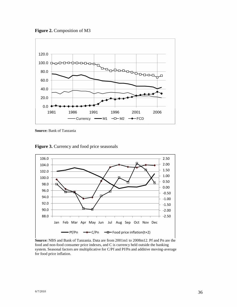
M3 is defined in Tanzania as M2 plus foreign currency deposits. The composition of

M3 (Figure 2) brings out two main observations. The first is the continued prominence of

currency – at 20 percent of M3 in 2008 – despite its gradual replacement by bank deposits.

Currency remains the dominant means of exchange in much of Tanzania, especially in rural

5 It is likely that the proportion bottomed out in the mid- to late-1990s, as NBC was being restructured and new banks had not yet established a substantial foothold. Reductions in rural access may well have lasted longer, however. The National Microfinance Bank, which succeeded NBC and acquired most of NBC‟s rural branch network, remained in state hands until 2005, operating for most of the 1997-2005 period under a private consulting contract that focused on enhancing profitability, not on expansion of reach or services. See Cull and Spreng (2008).

6/7/2010 7

areas.6 Figure 3 provides some evidence of the links between currency and rural

economic activity in Tanzania. The seasonal pattern of real currency holdings is very

strongly correlated with the seasonal in the monthly real price of food, where the latter is

defined as the food CPI deflated by the non-food CPI. Nyella (2005) suggests that these

co-movements are driven by the crop cycle, with currency holdings peaking at the time of

harvest (he also cites an end-of-year holiday spending effect).

The second feature of M3 is the growing importance of foreign-currency deposits

(FCDs), which peaked in 2006 at just above one third of the total. Kessy (2008) finds that

the share of FCDs in total deposits is an increasing function of expected depreciation and the

share of trade in GDP. Figure 4 compares the ex post yield on 12-month foreign currency

deposits with the interest rate on comparable domestic deposits over the past decade. For

most of the period FCD have constituted a favorable medium-term store of value for

households prepared to tolerate the volatility in their return. Key features

Our discussion has emphasized a set of potentially important features of the

Tanzanian case since the mid-1990s. These include

• a large share of currency in the higher monetary aggregates;

• a small share of the public with bank accounts, particularly in rural areas where

the economy remains largely cash-based;

• the coexistence of deposit dollarization with capital controls, potentially allowing

a higher degree of exchange-rate-based portfolio substitution within M3 than

between domestic and foreign bonds;

• the introduction of Treasury Bills in 1994, offering a high-yielding alternative to

bank deposits;

• significant structural change in the economy stemming from macroeconomic and

supply-side reforms which shifted economic activity towards more monetary-

intensive activities and;

6 While 10 percent of Tanzanian households reported a member with a bank account in 2007, this proportion was nearly 25 percent in Dar es Salaam. The figure for rural areas must therefore be well below 10 percent.

6/7/2010 8

• the transformation of the banking sector after 1992, which improved the quality of

bank services while potentially restricting access to banking services at least

initially. The reforms of 1988-94 changed the menu of financial assets and the character of the

banking sector. In our view, these reforms were fundamental enough that an investigation

of contemporary portfolio behavior should start in 1994 at the earliest. We also noted,

however, that velocity behaves very differently during the second half of the 1990s than

subsequently. In principle, the sharp change in money supply behavior starting in 1995

should assist in the econometric identification of the money demand equation. As we

have stressed, however, the disinflation period as a whole remains something of a puzzle.

Real money balances fell sharply and persistently, despite the absence of commensurate

movements in the conventional determinants of demand. Below we identify components

of the 𝒛𝒕 vector that perform strongly in the post-1998 sample while providing at least a

partial account of the collapse in real money demand during the second half of the 1990s. 3. Existing work on money demand in Tanzania

We briefly review the Tanzanian literature, beginning with work that preceded the first

application of modern time series methods by Randa (1999).

The early literature features a set of partial adjustment models applied to annual

data (Gerdes 1990, Maje 1992, Kihuale 1994, Mgonya 1997). Estimation samples start in

1967 and end in 1995 or earlier. These models incorporate a lagged dependent variable

but otherwise have very sparse dynamics, if any. They use expected inflation as the

opportunity cost of money, reflecting the undeveloped nature of the financial system and

the absence of interest-bearing alternatives to money. In the earliest study, Gerdes (1990)

introduces the key empirical themes of this literature: high income elasticities, even by

the standards of low-income countries; conventional but weak portfolio responses to

expected inflation; and controversies over the empirical stability of the estimated

relationships.

6/7/2010 9

These early contributions uniformly employed real GDP as the scale variable.

Using data from 1967 to 1985, Gerdes (1990) reported long-run income elasticities of

close to 2.0 for M1 and M2, against a benchmark of 0.5 from the Baumol-Tobin

transactions demand model and 1.0 from the quantity theory of money. In line with the

literature on low-income countries, he attributed these high elasticities to ongoing

monetization of the economy and the persistence of limitations on the menu of alternative

financial assets. Similar long run income elasticities were found in subsequent

applications, including prominently that of Maje (1992), who incorporated the number of

branches of the monopoly National Bank of Commerce (NBC) as a direct proxy for the

pace of monetization. The sign on this variable was positive, as expected, but was not

statistically significant.

The coefficients on expected inflation varied across applications, but they tended

to be small and were in most cases statistically insignificant. Starting with Maje (1992)

the time deposit rate was often included as a measure of the return to alternative assets

(M1) or as part of the own return on money (M2); point estimates were often

appropriately signed, but were uniformly small and imprecisely estimated. It was not

possible in this early literature to reject the hypothesis of a perfectly inelastic response of

money demand to interest rates.

Gerdes (1992), Maje (1992) and Mgonya (1997) all implemented Chow tests to

assess the stability of the money demand function, as did Kihuale (1994) who applied a

broader battery of tests using data from 1967 to 1990. Results were mixed; Gerdes and

Mgonya were unable to reject parameter stability, while Maje and Kihaule found

evidence of instability. While the latter finding was perhaps more plausible in a highly

controlled economy undergoing the stresses of financial repression, economic collapse,

and structural adjustment, the sources of instability were not carefully diagnosed. A

limitation of this early literature, moreover, is the difficulty of distinguishing genuine

parameter instability from slow equilibrium correction when the variables have stochastic

trends. More generally, conventional tests of significance can be misleading when the

variables are non-stationary, as emphasized in the time-series literature following Engle

and Granger (1987); a cointegration/error-correction framework is required to correctly

identify short- and long-run relationships and support accurate inference (Enders 2007).

6/7/2010 10

Randa (1999) established the standard for contemporary research by moving to

quarterly data (1974q1-1996q4), incorporating a role for currency substitution, and

applying modern time series methods. Randa focused on M0, M1 and M2; Nyella (1998)

applied similar methods to M3, using quarterly data from 1986q1 to 1997q4. The

hallmark of the modern time-series approach is two-fold: first, close attention to the

stationarity properties of the data and the resulting distinction between long-run

equilibrium relationships and short-run dynamics; and second, where feasible, the

adoption of a system-based approach in which multiple long-run relationships may exist

among the variables. We return to these themes in Section 4 below.

Moving to quarterly data requires interpolation of the scale variable, since the

GDP accounts are available only annually. Randa uses quadratic interpolation, which

does not require (or benefit from) the use of indicator variables available at quarterly

frequency. Using similar interpolation methods, Nyella uses gross national disposable

income (GNDI), which differs from GDP by the sum of net factor income and net

transfers, a quantity dominated by large and variable amounts of foreign aid.

Randa‟s second innovation was the incorporation of the rate of depreciation of the

black market exchange rate as a measure of opportunity cost for households with access

to assets denominated in foreign currency. Currency substitution was illegal until the

early 1990s, and it is still illegal for Tanzanian residents to hold offshore assets. The

foreign exchange black market was nonetheless active starting in the mid-1970s, and

there is considerable evidence that portfolio influenced the behavior of the parallel

premium during the 1970s and 80s (O‟Connell 1992).

Randa‟s specification omitted interest rates in favor of inflation and depreciation.

The Johansen method confirmed the presence of a single cointegration vector relating

real money balances, real GDP, inflation and depreciation. Interpreted as a money

demand function, all coefficients had the expected signs and were statistically significant.

Estimated income elasticities were higher for successively broader monetary aggregates,

a finding also characteristic of the earlier literature. In all cases, however, they were

markedly smaller than previous work had suggested (0.81, 0.96 and 1.11 for M0 M1 and

M2 respectively) and more in line with estimates for other countries. The inflation

elasticity of demand for money was negative, as expected (magnitudes 0.43, 1.08 and

6/7/2010 11

1.16 for M0, M1 and M2, respectively), as was the elasticity with respect to expected

depreciation.

Randa interprets stability in terms of existence of a cointegrated long-run money

demand relationship. His conclusion is that a stable set of demand functions exists despite

the economic and financial reforms that have taken place since late 1980s. Nyella (1998)

reports a similar finding for real M3 (M2 plus foreign currency deposits), using quarterly

data for 1986q1 to 1997q4. Nyella‟s specification incorporates a measure of the own

return on money, in the form of the time deposit rate adjusted by the ratio of these

deposits to M3. It also incorporates expected depreciation, which plays double duty as a

component of the own return on foreign currency deposits and an opportunity cost for

households with access to foreign currency and offshore deposits that are outside of M3.

Nyella (1998) innovates by incorporating a deterministic proxy for financial

liberalizations undertaken in the early 1990s. This proxy goes from zero to 1 when

foreign currency deposits are introduced in 1992, and from 1 to 2 when the government

T-bill market is introduced in 1994. This variable is constrained to lie in the cointegration

space, implying a sequence of two equal and permanent shifts in the long-run

relationship.

As in Randa (1999), Nyella‟s analysis supports the presence of a cointegration

vector with the characteristics of a long-run money demand function. At 0.58, however,

the income elasticity is extremely low by the standards of previous research. The own

rate of return has a positive and statistically significant impact as expected, and the

coefficient is large, at −3.7. Depreciation has a positive (0.9) and significant coefficient,

consistent with stronger substitution into domestic foreign currency deposits than into

other foreign assets when expected depreciation rises. Short run elasticities from the

error-correction representation of the money demand equation were plausibly signed in

most cases. 4. The demand for M2

We estimate the demand for the M2 aggregate and its two sub-components, currency and

deposits, using quarterly data on the variables identified in equation (1) above (see

Appendix 3 for details). Quarterly data are available for all monetary aggregates, prices,

6/7/2010 12

𝒕 𝒕

𝒕

جئ

interest rates and exchange rates. Data on the scale variables (real GDP and real GNE) are only available at an annual frequency. We interpolate these to a quarterly frequency

using an augmented version of the „proportional Denton interpolation‟ method.7

The modern approach to money demand starts by interpreting equation (1) as a

long-run equilibrium relationship. The deviation from this equilibrium should therefore

be a stationary random variable with a zero mean. Denoting the vector of determinants by

𝒊𝑨𝑳𝑻 , جئجئ = 𝒕جئ

, 𝒊جئ𝑾جئ

, 𝜋جئجئ , جئ ,

𝒛𝒕

′ , and assuming linearity, this implies

(2) , جئجئ + 𝒕جئ ′ جئ = جئجئ

where the „equilibrium error‟ جئ has a zero unconditional mean and constant unconditional variance and where the sub-vector 𝒛 may include deterministic components (e.g., a constant, a linear trend, seasonal dummy variables). We verify below that m and the

variables in w have unit roots (see Appendix 4). In this case the stationarity of جئ implies

that the variables are cointegrated. The long-run money demand coefficients correspond

to the cointegration vector 1, جئ ′ .

If there is only one long-run relationship between the variables in جئ , جئجئ′ , then

the long-run coefficients can be estimated consistently in a variety of ways, including

OLS as applied to equation (2). The short-run dynamics of the system can then be

recovered by estimating an error-correction specification in which the change in money

balances responds to current and lagged changes in the other variables as well as to the

previous period‟s estimated equilibrium error, جئ ′ جئ − 1− جئجئ𝒕−𝟏:

جئ = جئجئ∆ 𝒕−𝟏جئ ′ جئ − 1− جئجئ جئ − جئ− جئجئ∆ جئجئ 1= جئ

+

جئ (3) . جئجئ + 𝒕−𝒊جئ∆ ′ جئ 0= جئ

7 This method generates a smoothed interpolated quarterly series from annual data subject to the constraint that the sum over the year of the interpolated quarterly values for GDP equals the known annual total GDP. We augment this series by exploiting known quarterly movement in correlates of real GDP, such as trade flows and investment expenditure.

6/7/2010 13

Cointegration implies that the adjustment speed جئ lies between −2 and 0. While OLS

yields a consistent estimator of the adjustment speed, consistency of the other estimates

relies on weak exogteneity of the right-hand-side variables (Enders 2006).

In large samples, a systems approach is likely to be preferable to the Engle-

Granger two-step method we have just described. Starting with an unstructured vector ′ ′ autoregression involving the vector جئ𝒕 = جئ , جئجئ𝒕 , the Johansen method allows joint

estimation of the short- and long-run coefficients and provides an orderly approach to

assessing exogeneity and identifying multiple cointegrating relationships among the

variables (e.g., Juselius 2006). In the presence of a single cointegration vector, however,

the Engle-Granger two-step method tends to produce smaller bias in very small samples.

In what follows we rely on the two-step procedure, leaving systems estimation as a

potential extension. Incorporating structural change

As emphasized above, the money demand literature in Tanzania has tended to

feature income elasticities that are both very high and sensitive to the sample. The

standard explanation for high income elasticities in low-income countries is that increases

in aggregate income are accompanied by structural changes that increase the use of

currency and bank deposits in transactions. These changes can bias upwards the

measured income elasticity by conflating it with the impact of structural change.

While the „monetary intensity‟ of economic activity cannot be measured directly,

we can proxy it based on the set of measures depicted in Figure 5. Starting from the

activity side, we define the monetary-intensive share of GDP as the share of mining and

quarrying, manufacturing, electricity and water supply, trade, restaurants and hotels,

transport and communications, and finance, insurance and real estate. We then include

investment as a share of GDP and imports as a share of GDP, on the grounds that these

components of expenditure are more transactions-intensive than other components of

GDP. The government wage bill as a share of GDP is next; this has increased

substantially in recent years, reflecting increases in both real wages and employment

(including MDG-related spending). In contrast to much of the private sector, government

6/7/2010 14

wages and salaries are paid though the banking system. Finally, credit to the private

sector as a share of M3 provides a direct measure of banking sector intermediation.

These proxies tend to emphasize change in the demand for liquidity services.

Other things equal, reductions in the effective cost of acquiring financial services would

also serve to increase the monetary intensity of economic activity, and vice versa. To

date, however, it has not been possible to compute measures of these supply-side

changes, either directly in terms of the cost of access to financial services or indirectly

through measures of the changing structure and operations of the financial system as a

result of the reforms described in Appendix 1. We hope to develop such measures and

incorporate these in our measure of structural change in subsequent work.

While each of these variables captures a distinct aspect of the changing monetary

intensity of GDP, data limitations preclude our incorporating multiple proxies in our

regressions. We can summarize the information content in these measures, however, by

extracting their first principal component. Table 1 shows the results of this exercise.

There is a very strong commonality across the movements of these variables, such that a

more-or-less equally weighted average accounts for nearly three-quarters of their total

covariance. We use this weighed average as our proxy for transactions intensity. As

indicated in Figure 5, transactions intensity falls dramatically in the early stages of the

1995-99 disinflation, before stabilizing in the late 1990s and then rising sharply and

cumulatively starting around 2002. Long-run estimates

Table 2 shows our results for the long-run demand for M2, for samples beginning

in 1994q1 and 1998q1. Note that in all specifications a Dickey-Fuller test rejects the

hypothesis of a unit root in the residuals. Since the variables themselves are I(1), this is

evidence of cointegration. Results are somewhat stronger for real GDP than for real

GNE, and in subsequent tables we focus solely on specifications involving real GDP.

The results for the post-1998 sample appear in columns 3 and 4. The transactions

intensity of GDP comes in very strongly, and with this dimension of structural change

included in the regression, the expenditure and income elasticities – at 1.58 and 1.78

when transactions intensity is excluded – fall sharply. The scale elasticities are now

6/7/2010 15

insignificantly different from 1. Expected inflation and expected depreciation have the anticipated signs and reasonable magnitudes, with a 10 percent increase at an annual rate

reducing real money demand by 0.8 and 2.2 percent, respectively. 8

We noted earlier that an existing literature finds weak interest rate effects, based

mainly on samples ending in the mid-1990s or earlier. Perhaps surprisingly, this effect

persists after a decade of banking sector reforms. The spread between the T-bill rate and

the rate on time deposits has a plausible sign and magnitude in column 3, but neither

survives in column 4, and we cannot reject that the coefficient is zero in either case. At

least one of the centred seasonal dummies, in contrast, has a large and statistically

significant coefficient in each specification.

Figure 6 shows the cointegration relationship for the regression in column 4.

While real money balances and their determinants move closely together, the mean

squared error is substantial at 3.7 percentage points. Equilibrium errors are sizeable over

the 2005-2007 period, with a persistent under-prediction starting in 2005 followed by

over-prediction in 2007.

As shown in columns 1 and 2, cointegration survives but the fit deteriorates

markedly when the sample is extended back to 1994. The root mean squared errors rise

by roughly a third. Among the opportunity cost variables, only expected depreciation

continues to perform strongly, its significance intact and its magnitude roughly doubling.

The income elasticities are now significantly below unity. Short-run dynamics

In Table 3, we estimate dynamic error-correction models (ECMs) using the estimated

equilibrium errors from columns 2 and 4 of Table 2. Note that all variables in these

specifications are stationary – the equilibrium errors by virtue of cointegration, and the

remaining variables via differencing. Statistical tests suggest excluding the transactions

intensity variable from the short-run dynamics, and so we proceed accordingly. We focus

on the post-1998 sample (columns 2 and 3).

8 For all models we report heteroscedasticity-robust standard errors. Our interpolation of real GDP allows us to exploit a sample of approximately 40 observations. However, this masks the fact that we have only 11 independent observations on real GDP. To check that this does not seriously distort our interpolation, we also compute standard errors from a bootstrap routine. This slightly raises the estimated standard errors reported in the tables in this paper but not sufficiently to alter any inference we draw from the results.

6/7/2010 16

Column 2 shows an unrestricted ECM that includes one lag of all variables, and in

column 3 we reduce this to a parsimonious specification with stronger statistical

properties.9 The parsimonious specification generates a root mean squared error of 2.6

percentage points, by comparison with a standard deviation of the dependent variable of

3.6 percentage points per quarter. There is no evidence of serial correlation in the post-

1998 sample.

Error correction is an implication of cointegration, and so the negative and

statistically significant coefficient on the lagged equilibrium error is important

corroboration of our cointegration result. The speed of error correction is considerable, at

over 30 percent per quarter. At the same time the growth in real money balances displays

considerable short-run inertia, with a lag coefficient of roughly 0.3. Real GDP has a

smaller impact in the short run than it does over time, but the coefficient is strongly

significant. Inflation and depreciation both come in strongly in the short run; and the

interest-rate spread continues to be insignificantly different from zero. The seasonal

dummies remain large and important.

Figure 7 shows the actual and fitted values from the parsimonious ECM (column

3). The short-run dynamics go some way towards resolving the large and persistent

equilibrium errors in 2005-2007, with the exception of a single large outlier in the first

quarter of 2005. 5. Currency and deposits

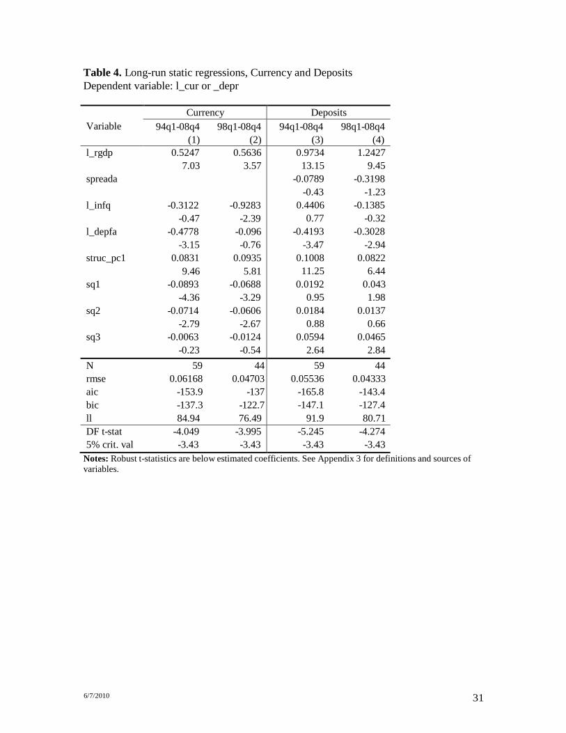
In Tables 4-6 we undertake a similar exercise for the two main components of M2,

currency and domestic-currency bank deposits. Our aim here is to shed some light on

compositional effects within M2. While these effects are present in any money demand

exercise, they may be of particular interest in Tanzania. The dominance of currency in

rural areas, the small proportion of the population with bank accounts, and the potentially

even smaller proportion with interest in or awareness of the T-bill market, suggests that

the relevant opportunity costs may differ sharply across the components of M2. The

9 Where appropriate we accommodate higher lags in the parsimonious specification.

6/7/2010 17

puzzle of largely-absent interest-rate effects, in particular, may in part be a result of

aggregation, if markets are partly segmented and only a portion of M2 responds to

interest rate differentials.

While the results should be considered preliminary, they suggest sharp and

intuitively appealing differences within M2. As earlier we focus on the post-1998 results.

In Table 4, long-run currency demand responds strongly to expected inflation and not at

all to interest rates (we exclude them on statistical grounds). Perhaps surprisingly,

expected depreciation also has a small and insignificant impact on currency demand. The

demand for deposits, in contrast, responds very strongly to expected depreciation,

consistent with substitution between domestic- and foreign-currency deposits within M3.

The point estimate on the interest rate spread (we use the T-bill rate minus a weighted

average of domestic-currency deposit rates), moreover, is considerably larger in the

deposit equation than in the overall M2 regression, and much closer to statistical

significance. The impact of expected inflation on deposits is small and statistically

insignificant. A weak response to interest rates remains a feature of the short-run

dynamics, however, and inflation appears to have at least as strong a short-run impact on

domestic-currency deposits as it does on currency (Tables 5 and 6) 6. Forecasting velocity

Forecasts of velocity play a central role in the Bank of Tanzania‟s policy framework.

Expressed in terms of growth rates, the definition of velocity (𝑉 = 𝑃جئ/جئ) implies that

(4) , 1+ جئجئ∆ − 1+ جئجئ∆ = 1+ جئجئ∆

where جئ is the log of velocity. The change in real money balances, in turn, is the difference between nominal money growth and inflation: ∆جئ = ∆logجئجئجئ∆ − جئ𝑃. The Bank of Tanzania‟s reserve-money program combines an inflation target (∆جئجئجئ𝑃1+ جئ = 𝜋) with a projection for real growth ∆جئ∆ = 1+ جئجئ , to yield an inflation-consistent growth rate for nominal money:

6/7/2010 18

(5) . 1+ جئجئ∆ − 𝜋 + جئ∆ = 1+ جئجئجئجئجئ∆

The velocity forecast ∆1+ جئجئ therefore directly affects the programmed growth rate for

M2.

Large forecast errors are potentially costly. Too high a projection for ∆جئ implies a

tighter policy stance than intended: failure to accommodate a higher-than-anticipated

money demand may drive inflation below target, while serving as a brake on real

economic activity. Too loose a projection may feed inflation or asset price bubbles, with

delayed adverse effects on the economy.

The Bank of Tanzania‟s current approach relies on extrapolation of recent trends

in velocity. This approach makes sense when velocity appears to be subject to relatively

slow-moving trends: as indicated in Figure 8, velocity has been falling at an average of

5.25 percent per year for almost a decade. There is substantial short-run volatility around

this average, however – the standard deviation of the year-on-year change is 6.1 percent.

In this section we briefly compare the Bank‟s trend-extrapolation methods with

alternative approaches based on the time-series behavior of velocity, including a VAR

incorporating the determinants of money demand. We end by discussing how information

from an econometric money demand equation can be used in a velocity-forecasting

exercise. We proceed in two steps, first looking at the within-sample performance of

alternative models and then considering their out-of sample forecasting properties. The

first of these steps is diagnostic: it allows us to assess and discuss the properties of

alternative models against the background of full information about the data. Within-sample performance

The BoT‟s approach is an example of a broader class of univariate forecasts that rely only

on the past behavior of velocity. In what follows we compare a set of univariate

approaches with a multivariate approach based on the variables in our money demand

equation. We begin with a pair of univariate models that assume a locally deterministic

path for velocity. With some oversimplification, these represent alternative

formalizations of what the BoT does in practice.

6/7/2010 19

(i) A rolling trend estimator assumes that velocity will return, next quarter, to the

seasonally-adjusted trend line it has followed over the recent past. For purposes of

comparison, we use a 3-year window. The rolling trend estimator for period t is

therefore the one-period-ahead extrapolation of a linear trend estimated over

quarters t−13 to t−1, with seasonal dummy variables included.

(ii) A moving average growth estimator extrapolates the growth rate of velocity,

rather than its level. A velocity forecast of this type features prominently in the

„McCallum rule‟ for base money growth (McCallum 1988). Maintaining our 3-

year window, we compute the moving average growth estimator for quarter t as

the value of velocity in quarter t−4, plus the average year-on-year growth in

velocity over quarters t−13 to t−1.

We also consider a pair of univariate models that treat the trend in velocity as

stochastic.

(iii) A simple random walk with drift (and deterministic seasonal effects) takes the

form

جئجئ 1= جئ 3 + جئ = جئجئ∆

جئجئ

(6) . جئجئ +

where the parameters are estimated over the full sample. This model has the well-

known property that the best estimate of velocity next period is its value this

period (after accounting for the estimated drift and seasonal determinants of

velocity).

(iv) A random walk with drift is a special case of a more general set of I(1)

models of which the stationary part may exhibit a combination of autoregressive

and/or moving average components. The Box-Jenkins method provides a set of

guidelines for identifying a parsimonious ARIMA model that „best‟ exploits the

6/7/2010 20

𝒕−𝟏

𝒕−𝟏

𝒕

observed autocorrelations and partial autocorrelations of a given time series.

Estimating over the period since 1998q1, we selected an ARIMA(1,1,2) model

with deterministic seasonal factors. This model takes the form:

+ جئ جئجئ 3 + 1− جئجئ∆ 1جئ + 0جئ = جئجئ∆ (7) . جئ 𝜃 + جئ 𝜃 + جئ

2− جئ 2 1− جئ 1 جئ جئ 1= جئ

Univariate forecasting models employ only the history of velocity itself. Our

money demand equation, however, suggests a natural multivariate alternative. Using r to

denote the non-income determinants of the demand for money, equation (3) can be

written as

𝛥1جئ + 0جئ = جئجئ 𝛥2جئ − 1− جئجئ 1جئ − 1− جئجئ جئ − 1− جئجئ 𝒓′ + ′ ′

(8) ,(جئ)جئ + 𝛥𝒓𝒕−𝟏 5جئ + 𝛥𝒓𝒕−𝟏 4جئ + 1− جئجئ𝛥 3جئ + جئجئ𝛥 2جئ

where for simplicity we have imposed a lag order of p = 1. Using the definition جئجئ =

equation (8) implies the velocity equation , جئجئ − جئجئ

𝛥1جئ + 0جئ− = جئجئ 𝛥2جئ + 1− جئجئ 1جئ − 1 − 1− جئجئ جئ − 1− جئجئ 𝒓′ + ′ ′

(9) . جئ جئ − 𝛥𝒓𝒕−𝟏 5جئ − 𝛥𝒓𝒕−𝟏 4جئ − 1− جئجئ𝛥 3جئ + 1جئ − جئجئ𝛥 2جئ − 1

Equation (9) can in turn be rewritten as a distributed lag model in which the level of

velocity depends on its own lags and on the current and lagged levels of the determinants

of money demand In effect, we can think of (9) as the first row in the structural

simultaneous equations system

𝒕−𝟏 + 𝝋𝒕 , (10)جئ جئ جئ = 𝒕جئجئ where the vector جئ𝒕 = جئجئ , جئجئ , 𝒓′ ′

includes velocity and the determinants of money

demand discussed above, and 𝝋 is a vector of structural disturbances.

Equation (10) is a structural simultaneous equations model, but as long as B is

invertible it will have a reduced-form VAR representation of the form

6/7/2010 21

𝒕−𝟏 + 𝝑𝒕 , (11)جئ جئ جئ = 𝒕جئ

where (جئ)جئ 1−جئ = جئ جئ and 𝜗1−جئ = جئ 𝜑جئ . Equation (11) is stochastically balanced, and

therefore can be estimated consistently in levels, as long as each I(1) variable in the VAR

is cointegrated with at least one other I(1) variable in the VAR – a condition our

cointegration analysis has established. The estimated VAR provides a basis for

multivariate forecasting of velocity – or, for that matter, of any element of the vector جئ𝒕 .

It constitutes our final forecasting model.

Table 7 and Figures 9a and 9b compare the within-sample properties of the four

univariate approaches and the VAR.10 We report two standard measures, the root mean

square error (RMSE) and the mean absolute error (MAE).11 Amongst the univariate models, the time-series models systematically out-perform those that treat the trend as locally deterministic. All models will fail to predict turning points in the data, but short-

lag time-series based models will „get back on track‟ more rapidly than deterministic-

trend models (this difference will increase the longer the time-span used to estimate the

local trend).

Figure 9b, which compares the goodness of fit of the preferred ARIMA model –

the best-fitting univariate model of velocity – with that of the VAR model, clearly shows

the substantial gains to conditioning the estimate of velocity on the full set of

determinants of money demand. Prediction errors are generally smaller and shorter-

lived. This increase in predictive accuracy is direct reflected in Table 7 where the root

mean square error of the VAR forecast is less than half that of the rolling trend (from

5.3percent per quarter to 2.4 percent per quarter) and more than one percentage point per

quarter lower than the „best fitting‟ univariate ARIMA model.

10 By construction, the rolling trend and McCallum rule forecasts differ from the time series model in one important sense. By construction, for the former the forecast at time t is based only on information up to time t-1. This contrasts with the time-series models where the predictive performance of the model at time t is conditional on data up to time t-1 but the parameters of the models are estimated on data for the whole sample t= 1...T. This distinction disappears when we compare out-of-sample forecast performance. 11 The RMSE is the most commonly used measure, having the property that it is measured in the same units as the dependent variable itself. The MAE is similarly measured. The RMSE is, however, more sensitive than the MAE to outlier errors: the squaring process gives disproportionate weight to very large errors. Hence if the cost of an error is roughly proportional to the size of the error, not the square of the error, then the MAE may be a more relevant criterion. Generally, however, these statistics will vary in unison.

6/7/2010 22

Out-of-sample forecasting

Next we compare the out-of-sample forecast performance of the same set of models. We

estimate each model over the sample period to 2006q4 and compute summary measures

of forecast performance over the period from 2007q1 to 2008q4, reporting both one-step-

ahead and, for the three time series models, dynamic 8-step-ahead forecasts for the period

2007q1 to 2008q4.12

Table 8 reports the forecast statistics which serve to reinforce the within-sample

evidence. In terms of one-step-ahead forecast performance, the time-series models again

dominate the deterministic-trend models while the velocity forecast from the VAR model

again exhibits a substantially lower forecast error than any of the univariate measures.

Conditioning on the determinants of money demand clearly and decisively enhances

forecast performance. This is so for both the one-step and multistep forecast even though

the latter are necessarily higher. Figure 10 illustrates the one-step-ahead forecast error

for three representative measures (the rolling trend, the ARIMA and the VAR model).

All three models initially under-predict velocity in the first two quarters of 2007 and

over-predict throughout the remainder of 2007 and into 2008, although the VAR again

shows lower deviation and more rapid error correction. Finally, Figures 11 plots the

multi-step forecast for velocity, estimated from the VAR, against the actual path of

velocity, illustrating the systematic over-prediction of velocity throughout late 2007 and

2008. 7. Conclusions and Implications for Monetary Policy

We have identified a well-behaved dynamic demand function for M2 in Tanzania for the

period from 1998 to the present and have shown how this model can be used to enhance

the forecasting of velocity. Real income growth and structural change continue to

12 A one-step-ahead forecast is generated by estimating the model on data up to period t and forecasting the outcome for t+1 The estimate for t+2 is obtained by using the same model but computing the forecast conditional on the actual data up to t+1. By contrast, an h-period-ahead forecast computes each successive forecast period from t+1 to t+8 without updating the data beyond that available at time t. Thus, in this case, the estimate for t+2 is obtained using the data up to period t and the forecast made at time t of the value of the data at t+1. Forecast errors are therefore cumulated as the horizon is extended.

6/7/2010 23

generate a strong underlying trend of financial deepening, and by separating these two

effects our results shed light on the high and variable income elasticities that have been a

feature of the Tanzanian literature. Conventional opportunity cost effects are present, but

as in the earlier literature they appear to be dominated by substitution between domestic-

currency and foreign–currency assets, and between money and inflation hedges.

Disaggregating currency and deposits, we find that currency responds more strongly to

expected inflation, and deposits to the interest-rate spread vis-à-vis T-bills, than does

overall M2.

While our results go some way towards resolving the puzzle of persistently

declining velocity during the disinflation of 1995-99, our empirical models deteriorate

markedly when the four years 1994q1-1997q4 are included in the sample. Further work

may well improve our account of this period, but for operational purposes our view is that

the BoT should base its statistical work on the later period.

A variety of extensions are of high priority. The first is to complement – or

replace – our single-equation analysis with a multivariate approach that allows an orderly

treatment of exogeneity issues and multiple long-run relationships. It remains to be seen

whether our short sample will support such an approach, but some of the most important

policy questions have to do with system-wide dynamics. For example, we have shown

clearly that expected inflation affects money demand; for policy purposes, the urgent

question is whether monetary disequilibrium affects future inflation. An integrated

treatment of money and inflation dynamics would be of considerable value.

A second extension is to apply the methods of this paper to M3. Kessy (2008)

finds considerable evidence of substitution within M3, and our results are consistent with

this. Understanding the behavior of overall M3 may be of considerable value, particularly

in advance of capital account is liberalization.

Velocity forecasts play a central role in the BoT‟s monetary policy framework, as

they do throughout much of Sub-Saharan Africa. We have shown, not surprisingly, that a

vector auto-regression model, based on our structural money demand equation,

substantially out-performs a variety of univariate approaches, both within-sample and

over a short out-of-sample horizon. Thus, for short-term forecasting purposes, the

existence of a stable cointegrating relationship between real money balances – or velocity

6/7/2010 24

-and the determinants of money demand suggests that VAR-based forecasts, based on

the most up-to-date data, may have substantial value in program formulation, as a

complement to judgment and a check on simple univariate extrapolation.

6/7/2010 25

References

Bevan, David, Paul Collier and Jan Willem Gunning (1993) Controlled Open Economies: A Neoclassical Approach to Structuralism (Oxford: Clarendon Press)

Čihák, Martin and Richard Podpiera 2005 “Bank Behavior in Developing Countries:

Evidence from East Africa” IMF Working Paper 05/129 Washington, DC: International Monetary Fund, June

Cull, Robert and Connor Spreng 2008 “Pursuing Efficiency While Maintaining Outreach:

Bank Privatization in Tanzania” World Bank Policy Research Working Paper 4804 Washington, DC: The World Bank

Collier, Paul and Jan Willem Gunning (1991), ”Money Creation and Financial

Liberalization in A Socialist Banking System: Tanzania 1983-88” , World Development. 19(5), 533-538

Enders, Walter (2007) Applied Econometric Time Series 2nd Edition, Wiley, New York

Ericsson, Neil R. (1998), “Empirical Modeling of Money Demand” Empirical Economics

23: 295-315 Freedman, Charles and Douglas Laxton (2009), Why Inflation Targeting? IMF Working

Paper 09/86, April. Gerdes, William (1990), “The Demand for Money in Socialist Tanzania” Atlantic

Economic Journal 18(3), September Hall, Stephen, G. Hondroyiannis, P. Swamy, and G. Tavlas (2009) “Where Has All the

Money Gone? Wealth and the Demand for Money in South Africa” Journal of African Economies 18: 84 – 112

Honohan, Patrick and Torsten Beck (2007) Making Finance Work for Africa World

Bank, Washington, DC Juselius, Katarina (2006) The Cointegrated VAR Model: Methodology and Applications

Oxford: Oxford University Press Kessy, Pantaleo (2008) “Empirical Evidence on the Determinants of Dollarization in

Tanzania” Bank of Tanzania, Directorate of Economic Policy, May Kihaule, M.K. (1994) “Behaviour of Demand for Money: a case of Tanzania”

Unpublished dissertation, Department of Economics, University of Dar es Salaam, Tanzania

6/7/2010 26

Maje, E.H. (1992) “Monetization, Financial Development and the Demand for Money: The Case of Tanzania” Unpublished dissertation, Department of Economics, University of Lund (Lund, Sweden)

McCallum, Bennett (1988), “Robustness Properties of a Monetary Rule”, Carnegie-

Rochester Conference Series for Public Policy 29, Autumn: 173-203. Mgonya, B. (1997) “Demand for Money and Inflation in Tanzania 1966-1995”

Unpublished dissertation, Department of Economics, University of Dar es Salaam, Tanzania

Mwase, Nkunde and Benno J. Ndulu (2007), “Tanzania” in B. J. Ndulu et al., eds, The

Political Economy of Economic Growth in Africa, 1960-2000, Volume 1 (Cambridge: Cambridge University Press)

Ndanshau, M. (1996) “The Behaviour of Income Velocity in Tanzania, 1967-1994” African

Economic Research Consortium, Nairobi Ndulu, Benno J. (1997), “The Challenging Path of Transition to a Low Inflation Economy in

Tanzania” The Second Gilman Rutihinda Memorial Lecture (Dar es Salaam, Bank of Tanzania).

Nyella, Johnson J. (2005) “Seasonality of Currency in Circulation in Tanzania” Bank of

Tanzania Technical Commentaries and Observations 08/2005 Dar es Salaam: Bank of Tanzania

Nyella, Johnson (2003), “Financial Programming: The Case of Tanzania” Dar es Salaam:

Bank of Tanzania Nyella, Johnson (1998) “The Demand for Money in Tanzania” Dar es Salaam: Bank of

Tanzania O‟Connell, Stephen A. (1995), “Monetary Adjustment and Policy Compatibility in a

Controlled Open Economy” Journal of African Economies 4(1): 52-82 Parastatal Sector Reform Commission (2000), The 1999/2000 Review and the Action

Plan for 2000/2001, Government Printer, Dar es Salaam Randa, John (1999), “Economic Reform and the Stability of the Demand for Money in

Tanzania” Journal of African Economies 8(3): 307-344 Rashidi, Idris (1997), “Keynote Address to the 10th Conference of Financial Institutions: 7-9

April 1997, Arusha” in Bank of Tanzania Economic and Operations Report for the Year Ended 30th June 1997: 52-58

Siram, Subramanian (2001) “A Survey of Recent Empirical Money Demand Studies” IMF Staff

Papers 47(3): 334-65

6/7/2010 27

Waigama, Samuel M.S. (2008) Privatization Process and Asset Valuation: A Case Study of

Tanzania Doctoral Dissertation, School of Architecture and the Built Environment, Royal Institute of Technology, Stockholm, Sweden

Walsh, Carl E. (20!0)Monetary Theory and Policy, 3'd edition (Cambridge, MA: MIT Press)

6/7/2010 28

Tables and Figures

Table 1. Principal components analysis, 1994q1-2008q4 Number of observations: 59 Number of components: 5

1. Principal components

Component Eigenvalue Difference Proportion Cumulative Comp1 3.6546 2.8040 0.7309 0.7309 Comp2 0.8505 0.4151 0.1701 0.9010 Comp3 0.4354 0.4026 0.0871 0.9881 Comp4 0.0329 0.0063 0.0066 0.9947 Comp5 0.0266 . 0.0053 1.0000

2. Weights in first principal component, and descriptive statistics Variable Weights Mean Std. Dev. Min Max gwssh 0.4233 0.0398 0.0060 0.0342 0.0562 ytishr 0.4096 0.3778 0.0186 0.3480 0.4123 dcpm3 0.4738 0.3541 0.1118 0.1482 0.5802 gfcfgdp_di 0.5002 0.1927 0.0317 0.1492 0.2516 impgdp_di 0.4224 0.2759 0.0629 0.2065 0.3826

Notes: “Weights‟ is the eigenvector that constitutes the first principal component. See Appendix 3 for definitions and sources of variables.

6/7/2010 29

Variable 1994q1-2008q4 1998q1-2008q4 (1) (2) (3) (4)

l_rgne 0.6809 1.1111 7.53 7.49

l_rgdp 0.863 1.0169 12.14 8.22

spreada 0.0641 0.1194 -0.2734 0.0176 0.31 0.61 -1.01 0.08

l_infq -0.1543 0.2516 -0.783 -0.3383 -0.24 0.46 -1.67 -0.92

l_depfa -0.5252 -0.4707 -0.2415 -0.2713 -4.55 -4.14 -2.14 -3.23

struc_pc1 0.0957 0.0896 0.0607 0.0841 7.61 10.06 3.66 6.68

sq1 -0.0269 -0.0155 0.0015 0.0066 -1.29 -0.91 0.06 0.38

sq2 -0.0357 -0.0064 -0.0446 -0.0084 -1.48 -0.32 -1.99 -0.46

sq3 0.0018 0.0402 -0.0009 0.0274 0.06 1.90 -0.04 2.15

N 59 59 44 44 rmse 0.06199 0.05062 0.047 0.03727 aic -152.5 -176.4 -136.3 -156.7 bic -133.8 -157.7 -120.2 -140.6 ll 85.23 97.18 77.13 87.35 DF t-stat -3.961 -5.08 -4.198 -3.944 5% crit. val -3.43 -3.43 -3.43 -3.43

Table 2. Long-run static regressions, M2 Dependent variable: l_m2r

Notes: Robust t-statistics are below estimated coefficients. See Appendix 3 for definitions and sources of variables.

6/7/2010 30

Table 3. Dynamic ECM regressions, M2 Dependent variable: D.l_m2r

Variable 94q1-08q4 1998q1-2008q4

(1) (2) (3) L.equi_err -0.3405 -0.3324 -0.3294

-2.88 -2.52 -3.28 LD.l_m2r 0.3398 0.3103 0.3039

2.82 1.58 1.70 D.l_rgdp 0.126 0.4317 0.4355

1.03 2.29 3.00 LD.l_rgdp -0.1616 -0.0084

-1.33 -0.08 D.spreada 0.0631 -0.0719

0.64 -0.27 LD.spreada -0.0047 0.1086

-0.04 0.51 D2.spreada -0.0862

-0.58 D.l_infq -0.3235 -0.5002 -0.5087

-1.2 -1.84 -2.71 LD.l_infq 0.0818 0.0191

0.37 0.10 D.l_depfa -0.0533 -0.0862 -0.0847

-0.83 -1.66 -1.87 LD.l_depfa 0.1836 0.0084

1.93 0.06 sq1 -0.0322 -0.0145 -0.0147

-2.22 -0.86 -1.06 sq2 0.018 0.0102 0.0095

1.32 0.46 0.50 sq3 0.0322 0.0432 0.0424

2.12 2.4 2.62 N 58 42 42 Rmse 0.02895 0.02525 0.02364 Aic -234.3 -178.9 -186.8 Bic -205.5 -154.5 -169.4 Ll 131.2 103.4 103.4 P-values Res normality 0.05 0.001 0.001 BP Het 0.038 0.008 0.009 BG Auto lag1 0.45 0.878 0.997 lag2 0.016 0.281 0.367 lag3 0.014 0.106 0.166 lag4 0.009 0.181 0.271

Note: l.equi_err is the lagged equilibrium error from the static regression in column 2 or 4 of Table 2.

6/7/2010 31

Table 4. Long-run static regressions, Currency and Deposits Dependent variable: l_cur or _depr

Variable

Currency Deposits 94q1-08q4 98q1-08q4

(1) (2) 94q1-08q4 98q1-08q4

(3) (4) l_rgdp 0.5247 0.5636

7.03 3.57 spreada

l_infq -0.3122 -0.9283

-0.47 -2.39 l_depfa -0.4778 -0.096

-3.15 -0.76 struc_pc1 0.0831 0.0935

9.46 5.81 sq1 -0.0893 -0.0688

-4.36 -3.29 sq2 -0.0714 -0.0606

-2.79 -2.67 sq3 -0.0063 -0.0124

-0.23 -0.54

0.9734 1.2427 13.15 9.45

-0.0789 -0.3198 -0.43 -1.23

0.4406 -0.1385 0.77 -0.32

-0.4193 -0.3028 -3.47 -2.94

0.1008 0.0822 11.25 6.44

0.0192 0.043 0.95 1.98

0.0184 0.0137 0.88 0.66

0.0594 0.0465 2.64 2.84

N 59 44 rmse 0.06168 0.04703 aic -153.9 -137 bic -137.3 -122.7 ll 84.94 76.49

59 44 0.05536 0.04333

-165.8 -143.4 -147.1 -127.4

91.9 80.71 DF t-stat -4.049 -3.995 5% crit. val -3.43 -3.43

-5.245 -4.274 -3.43 -3.43

Notes: Robust t-statistics are below estimated coefficients. See Appendix 3 for definitions and sources of variables.

6/7/2010 32

Table 5. Dynamic ECM regressions, Currency Dependent variable: D.l_cur

Variable 94q1-08q4 1998q1-2008q4

(1) (2) (3) L.equi_err -0.3942 -0.4971 -0.5196

-3.31 -2.71 -3.12 LD.l_cur 0.1872 0.2184 0.2192

1.37 1.11 1.43 D.l_rgdp 0.2399 0.4336 0.4432

2.06 1.71 1.76 LD.l_rgdp -0.1359 0.0676

-1.31 0.35 D.l_ifwd2a -2.1789 -7.5882 -5.5459

-1.87 -1.78 -1.82 LD.l_ifwd2a 2.0943 3.1821

1.48 0.77 D.l_infq -0.6995 -0.97 -0.8423

-2.06 -2.46 -2.88 LD.l_infq -0.1824 -0.198

-0.57 -0.56 D.l_depfa -0.1246 -0.1309

-1.44 -1.14 LD.l_depfa 0.3162 0.2672

2.00 1.07 D2.l_depfa -0.1956

-1.59 sq1 -0.1029 -0.0856 -0.0848

-5.92 -2.88 -3.07 sq2 0.0153 0.0202 0.0267

0.48 0.57 0.77 sq3 0.0403 0.026 0.0367

2.13 1.00 1.78 N 58 42 42 Rmse 0.03878 0.0409 0.03898 Aic -200.4 -138.3 -144.8 Bic -171.6 -114 -127.4 Ll 114.2 83.17 82.39 P-values Res normality 0.576 0.516 0.647 BP Het 0.811 0.955 0.766 BG Auto lag1 0.096 0.131 0.25 lag2 0.233 0.071 0.06 lag3 0.391 0.135 0.124 lag4 0.091 0.196 0.201

Note: l.equi_err is the lagged equilibrium error from the static regression in column 1 or 2 of Table 3.

6/7/2010 33

Table 6. Dynamic ECM regressions, Deposits Dependent variable: D.l_depr

Variable 94q1-08q4 1998q1-2008q4

(1) (2) (3) L.equi_err -0.3343 -0.2714 -0.3196

-2.59 -2.20 -3.55 LD.l_depsr 0.4298 0.2856 0.3074

3.86 1.98 2.31 D.l_rgdp 0.0948 0.3906 0.4168

0.70 2.21 3.26 LD.l_rgdp -0.1463 0.0235

-1.09 0.15 D.spreada -0.0391 -0.2947 -0.2747

-0.34 -1.02 -1.32 LD.spreada 0.0695 0.2656

0.56 1.69 D.l_infq -0.2924 -0.4104 -0.4302

-1.13 -1.50 -2.07 LD.l_infq 0.0192 0.0073

0.09 0.04 D.l_depfa -0.0322 -0.0713 -0.0718

-0.41 -1.12 -1.14 LD.l_depfa 0.1338 -0.0892

1.08 -0.53 sq1 0.0092 0.0158 0.019

0.61 1.11 1.49 sq2 0.0067 -0.0057 -0.0099

0.53 -0.33 -0.79 sq3 0.0308 0.0417 0.0382

1.95 2.49 2.62 N 58 42 42 Rmse 0.03289 0.02746 0.0263 Aic -219.5 -171.8 -177.8 Bic -190.7 -147.5 -160.5 Ll 123.8 99.91 98.92 P-values Res normality 0.027 0.001 0.001 BP Het 0.765 0.977 0.929 BG Auto lag1 0.817 0.19 0.768 lag2 0.028 0.222 0.142 lag3 0.016 0.084 0.083 lag4 0.009 0.109 0.139

Note: l.equi_err is the lagged equilibrium error from the static regression in column 3 or 4 of Table 3.

6/7/2010 34

Table 7. Velocity: within-sample predictive performance Sample 2002q1 to 2008q4

Model (dependent variable log velocity) RMSE

( % per quarter)

MAE

(% per quarter)

Rolling Trend 5.26 4.47

Seasonal Moving Average 6.66 5.16

Random walk with seasonals 4.09 3.13

SARIMA (1,1,2,4) 3.61 2.92

VAR (2) 2.42 1.70

Notes: Measures indicate the accuracy of the within-sample predictive power of the model, where for each model the prediction error is [(جئ)جئ − جئ جئ] = جئ جئ. RMSE is the root mean square error; MAE the mean absolute error. SARIMA denotes seasonal autoregressive integrated moving average of order p=1, d=1, q=2 and s=4 where p denotes the autoregressive order, d the order of integration, q the moving average error order and s the number of deterministic seasonal dummy variables. VAR(2) denotes vector auto-regression with two lags on each variable (plus deterministic seasonal dummy variables).

Table 8. Velocity: out-of-sample forecast performance Estimation Sample 1998q1 to 2006q4 Forecast Sample 2007q1 to 2008q4

Model (dependent variable log velocity)

1-step-ahead forecast

(% per quarter)

8-step-ahead forecast

(% per quarter) RMSE MAE RMSE MAE

Rolling Trend 6.04 5.61

Seasonal Moving Average 7.67 6.99

Random walk w/ seasonals 3.76 3.20

SARIMA (1,1,2,4) 4.05 3.05

VAR (2) 2.51 2.11

- -

- -

7.45 6.95

7.31 6.86

5.13 4.54

Notes: See Table 7 and text.

6/7/2010 35

1.2

1.4

1.6

1.8

2.2

2 4.

5 5.

5 6.

5 4

5 6

0 20

40

60

0

10

20

30

40

50

1.2

1.4

1.6

1.8

2.5

3.5

.8

1 2

3

10

20

30

4

0

50

0 20

40

60

Figure 1. Velocity of monetary aggregates, 1988q1-2008q4

Velocity of monetary aggregates, 1988Q1-2008Q4

cu m1

1990q1 1995q1 2000q1 2005q1 2010q1 1990q1 1995q1 2000q1 2005q1 2010q1

m2 m3

1990q1 1995q1 2000q1 2005q1 2010q1 1990q1 1995q1 2000q1 2005q1 2010q1

Blue: Velocity (Left) Red: Y/Y Money Growth (Right)

Source: Bank of Tanzania

6/7/2010 36

Figure 2. Composition of M3

120.0

100.0

80.0

60.0

40.0

20.0

0.0 1981 1986 1991 1996 2001 2006

Currency M1 M2 FCD

Source: Bank of Tanzania Figure 3. Currency and food price seasonals

106.0

104.0

102.0

100.0

98.0

96.0

94.0

92.0

90.0

88.0

Jan Feb Mar Apr May Jun Jul Aug Sep Oct Nov Dec

2.50 2.00 1.50 1.00 0.50 0.00 -0.50 -1.00 -1.50 -2.00 -2.50

Pf/Pn C/Pn Food price inflation(t+2)

Source: NBS and Bank of Tanzania. Data are from 2001m1 to 2008m12. Pf and Pn are the food and non-food consumer price indexes, and C is currency held outside the banking system. Seasonal factors are multiplicative for C/Pf and Pf/Pn and additive moving-average for food price inflation.

6/7/2010 37

3)

.34

.36

.38

.42

.1

.2

.3

.4

.5

.6

.4

%

Jun-

99

Nov

-99

Apr

-00

Sep-

00

Feb-

01

Jul-0

1 D

ec-0

1 M

ay-0

2 O

ct-0

2 M

ar-0

3 A

ug-0

3 Ja

n-04

Ju

n-04

N

ov-0

4 A

pr-0

5 Se

p-05

Fe

b-06

Ju

l-06

Dec

-06

May

-07

Oct

-07

Mar

-08

Aug

08

.035

.0

45

.055

.0

4 .0

5 .1

5 .2

5 .2

.25

.35

-2

.2

.3

.4

0 2

4

Figure 4. Ex post yields on domestic and foreign currency deposits

25

20

15

10

5

0

-5

-10

Expected return on FCD DC_12m_td rate

Source: Bank of Tanzania

Figure 5. Structural Change and the Monetary Intensity of Economic Activity.

Indicators of monetary intensity of economic activity

1994Q4 to 2008Q4

Modern share of GDP Investment (% GDP)

Imports (%GDP)

1995q1 2000q1 2005q1 2010q1 1995q1 2000q1 2005q1 2010q1 1995q1 2000q1 2005q1 2010q1

Domestic credit to private sector (%M Govt wage bill (%GDP) Principal Component Analysis

1995q1 2000q1 2005q1 2010q1 1995q1 2000q1 2005q1 2010q1 1995q1 2000q1 2005q1 2010q1

Note: See Table 1 for details on the principal components calculation.

6/7/2010 38

Line

ar p

redi

ctio

n Li

near

pre

dict

ion

10.5

-.2

-.1

9.

5 .1

.2

10

0

9

Figure 6. Long-run equilibrium: actual and fitted values

Tanzania log real Money M2 1998q1 to 2008q4 Actual vs Fitted

1998q1 2000q1 2002q1 2004q1 2006q1 2008q1 time

+/- 2s.e. fitted log real M2

Scale variable: rgdp

Source: Column 4 of Table 2.

Figure 7. Short-run dynamics: actual and fitted values

Tanzania log real Money M2 1998q1 to 2008q4

Actual vs Fitted

1998q1 2000q1 2002q1 2004q1 2006q1 2008q1 time

+/- 2s.e. fitted growth in log real M2

Scale variable: rgdp

Source: Column 3 of Table 3.

6/7/2010 39

20

40

60

80

0 -15

-10

-5

0 5

Figure 8. Time-series forecasts of M2 velocity

Log M2 velocity 1998q1 to 2008q4

1998q1 2000q1 2002q1 2004q1 2006q1 2008q1 time

log velocity [LHS] Quarter on Quarter change in velocity [RHS]

Source: Bank of Tanzania.

6/7/2010 40

-10

-10

-5

10

-5

10

0 5

0 5

Figure 9. Velocity forecasting models: within-sample performance (a) Rolling trend forecaster vs random walk

Log M2 velocity 2004q1 to 2008q4

Within sample prediction error

2004q1 2005q1 2006q1 2007q1 2008q1 2009q1 time

Rolling Trend Random Walk (b) ARIMA versus VAR

Log M2 velocity 2004q1 to 2008q4

Within sample prediction error

2004q1 2005q1 2006q1 2007q1 2008q1 2009q1 time

ARIMA VAR

6/7/2010 41

Perc

ent

10

20

30

40

-10

-5

10

0 0

5

Figure 10. One-step-ahead forecast error from alternative forecast models

Log M2 velocity out-of-sample forecast performance One-step-ahead forecast errors

2006q1 2006q3 2007q1 2007q3 2008q1 2008q3 time

Rolling Trend SARIMA VAR

Figure 11. Actual velocity versus 8-step ahead VAR-based forecast

Log M2 velocity: 2007q1 to 2008q4 VAR-based dynamic forecast

2006q3 2007q1 2007q3 2008q1 2008q3

95% CI forecast observed

6/7/2010 42

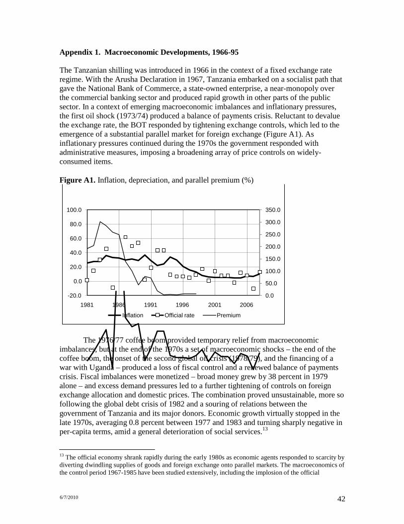
Appendix 1. Macroeconomic Developments, 1966-95 The Tanzanian shilling was introduced in 1966 in the context of a fixed exchange rate regime. With the Arusha Declaration in 1967, Tanzania embarked on a socialist path that gave the National Bank of Commerce, a state-owned enterprise, a near-monopoly over the commercial banking sector and produced rapid growth in other parts of the public sector. In a context of emerging macroeconomic imbalances and inflationary pressures, the first oil shock (1973/74) produced a balance of payments crisis. Reluctant to devalue the exchange rate, the BOT responded by tightening exchange controls, which led to the emergence of a substantial parallel market for foreign exchange (Figure A1). As inflationary pressures continued during the 1970s the government responded with administrative measures, imposing a broadening array of price controls on widely- consumed items.

Figure A1. Inflation, depreciation, and parallel premium (%)

100.0

80.0

60.0

40.0

20.0

0.0

350.0 300.0 250.0 200.0 150.0 100.0 50.0

-20.0

1981 1986 1991 1996 2001 2006

Inflation Official rate Premium

0.0

The 1976/77 coffee boom provided temporary relief from macroeconomic imbalances, but at the end of the 1970s a set of macroeconomic shocks – the end of the coffee boom, the onset of the second global oil crisis (1978/79), and the financing of a war with Uganda – produced a loss of fiscal control and a renewed balance of payments crisis. Fiscal imbalances were monetized – broad money grew by 38 percent in 1979 alone – and excess demand pressures led to a further tightening of controls on foreign exchange allocation and domestic prices. The combination proved unsustainable, more so following the global debt crisis of 1982 and a souring of relations between the government of Tanzania and its major donors. Economic growth virtually stopped in the late 1970s, averaging 0.8 percent between 1977 and 1983 and turning sharply negative in per-capita terms, amid a general deterioration of social services.13

13 The official economy shrank rapidly during the early 1980s as economic agents responded to scarcity by diverting dwindling supplies of goods and foreign exchange onto parallel markets. The macroeconomics of the control period 1967-1985 have been studied extensively, including the implosion of the official

6/7/2010 43

A maxi-devaluation in 1983, undertaken in the midst of deep macroeconomic difficulties, marked the beginning of what ultimately proved a decisive transition from direct controls to price-based mechanisms of macroeconomic adjustment in Tanzania. President Nyerere resigned in 1985, and in the following year the country embarked on a sequence of 3-year Economic Recovery Programmes (ERP I, 1986-89, and ERP II, 1989- 92) with IMF and World Bank support. These were designed to convert an administratively controlled economy into one with market-determined prices and private ownership and control. Over the course of a decade, these reforms transformed the banking sector and the menu of financial assets available to Tanzanian households.

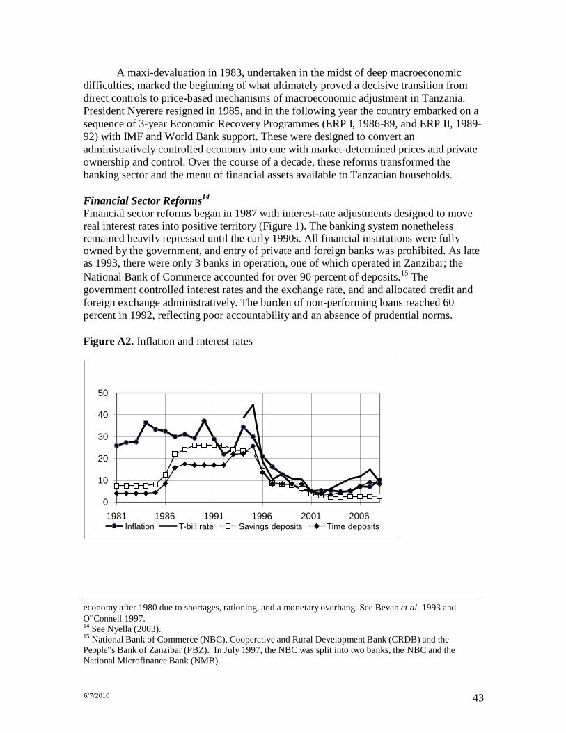
Financial Sector Reforms14

Financial sector reforms began in 1987 with interest-rate adjustments designed to move real interest rates into positive territory (Figure 1). The banking system nonetheless remained heavily repressed until the early 1990s. All financial institutions were fully owned by the government, and entry of private and foreign banks was prohibited. As late as 1993, there were only 3 banks in operation, one of which operated in Zanzibar; the National Bank of Commerce accounted for over 90 percent of deposits.15 The government controlled interest rates and the exchange rate, and and allocated credit and foreign exchange administratively. The burden of non-performing loans reached 60 percent in 1992, reflecting poor accountability and an absence of prudential norms.

Figure A2. Inflation and interest rates

50

40

30

20

10

0 1981 1986 1991 1996 2001 2006

Inflation T-bill rate Savings deposits Time deposits

economy after 1980 due to shortages, rationing, and a monetary overhang. See Bevan et al. 1993 and O‟Connell 1997. 14 See Nyella (2003). 15 National Bank of Commerce (NBC), Cooperative and Rural Development Bank (CRDB) and the People‟s Bank of Zanzibar (PBZ). In July 1997, the NBC was split into two banks, the NBC and the National Microfinance Bank (NMB).

6/7/2010 44

Following the Nyirabu Commission‟s report in 1990, the government undertook a sequence of reforms that transformed an insolvent nationalized monopoly banking system into an increasingly competitive sector dominated by foreign-owned banks (Cull and Spreng 2008). The process began with the entry of the first private foreign banks in 1992 and 1993 (they began operations in 1994) and the privatization of the Cooperative and Rural Development Bank (CRDB) in 1996. The dominant National Bank of Commerce (NBC) was recapitalized in successive efforts during the early and mid-1990s, and in 1997 the Government divided it into the new NBC, which inherited the bank‟s urban branches and its traditional urban- and trade-based lending business, and the National Microfinance Bank (NMB) which inherited the old NBC‟s network of rural branches and its mandate to provide banking services to rural populations. The new NBC was privatized in 2000, and the NMB went 0 to 49% private participation in 2005.

The introduction of competition transformed the quality, price, and availability of banking services in Tanzania, with potentially large impacts on the demand for bank liabilities. The evidence suggests substantial increases in bank profitability and efficiency. The restructuring process also appears to have restricted the access of households to financial services, however, at least initially and particularly in rural areas; the NBC retrenched 2,800 employees and closed 23 branches in 1994 alone. Successive household budget surveys show a sharp decrease during the 1990s in the proportion of households reporting a bank account – this number falls from 18.0 percent in the 1991/92 survey to 6.4 percent in 2000/01, before recovering to 10.0 percent in the 2007 survey.16

But the Banking and Financial Institutions Act of 1991 authorized the entry of private and foreign banks, and in 1994 the first two (Standard Chartered and Meridien–BIAO, both foreign-owned) began operations. By the end of 2001, the total number of banks had reached 17; this number doubled again by 2009, with the majority of Tanzania‟s 34 banks foreign-owned., along with a possible reduction in access to financial services in rural areas, for example through the closure of branches when NBC was split (Cihak and Podpiera 2005). The rapid introduction of mobile banking and other technological innovations over the past 5 years or so has further transformed the menu of banking services available in Tanzania.

A set of contemporaneous reforms during the early 1990s converted a system of exchange controls and multiple exchange rates into one in which private residents were allowed to hold foreign currency and domestic foreign-currency deposits and exchange rates were determined in an inter-bank market. The Foreign Exchange Act of 1992 introduced privately-owned foreign exchange shops and allowed residents to hold foreign currency deposits for the first time. A weekly foreign exchange auction system was introduced by the BOT in 1993, with the official exchange rate determined by the marginal market clearing bid; as intended, this was replaced in June 1994 by the Inter-bank Foreign Exchange Market (IFEM).

16 It is likely that the proportion bottomed out in the mid- to late-1990s, as NBC was being restructured and new banks had not yet established a substantial foothold. Reductions in rural access may well have lasted longer, however. The National Microfinance Bank, which succeeded NBC and acquired most of NBC‟s rural branch network, remained in state hands until 2005, operating for most of the 1997-2005 period under a private consulting contract that focused on enhancing profitability, not on expansion of reach or services. See Cull and Spreng 2008.

6/7/2010 45

Monetary and fiscal developments The early 1990s saw a gradual shift from direct to indirect instruments of monetary control, facilitated by interest rate liberalization and the introduction of Treasury bill auctions in 1993. The ERPs emphasized macroeconomic stabilization and introduced annual money-growth targets as a means of inflation control. Inflation remained persistently high, however, as fiscal pressures drove money growth rates well above program targets (Figure 1). Thus M2 growth averaged 32.4 percent during the reform period, as against the target range of 10 to 17 percent, the difference largely reflecting government borrowing to finance crop authorities and cooperative unions (Ndanshau 1996).

Monetary accommodation continued over the five-year period following the 1990 general elections. In a context of expansionary fiscal policy, the growth rate of extended broad money averaged 36.3 percent and inflation averaged nearly 30 percent (Figure 2). By 1994/95, sharply rising interest costs had convinced the policy authorities that fiscal adjustment was essential for macroeconomic stabilization (Rashidi, 1997).

Figure A3. Inflation and money growth

50.0

40.0

30.0

20.0

10.0

0.0 1981 1986 1991 1996 2001 2006

Inflation M2 M3

The conduct of monetary and fiscal policy changed abruptly in 1995. The Bank of Tanzania Act placed price stability first among the objectives of monetary policy and granted the BOT the independence required to carry out its role and functions. The government adopted a cash budget, accepting a virtually complete denial of monetary finance. As the cash budget and reserve money programs gained traction, the growth rate of extended broad money fell sharply, averaging 13.2 percent for the five year period ending 2000. Disinflation was rapid; inflation fell from 30% in 1995 to 16% in 1997 and below 10% in 1999 (Figure A3).

6/7/2010 46

جئ جئ جئ

جئ جئ

1− جئ جئ جئ

جئ جئ

Appendix 2. Motivating the demand for money The demand for any monetary aggregate can be motivated by reference to the portfolio problem of the household sector (e.g., Walsh 2010).

The end-of-period financial wealth of the private non-bank sector is given by

(A2.1) , $جئ جئجئ + جئجئ + $جئ جئجئ + جئجئ + $جئ جئجئ + جئجئ where C and D refer to cash and bank deposits, E is the exchange rate in Tanzanian shillings per US dollar, $ denotes holdings in foreign currency, and B denotes bonds, which on the domestic side are restricted to government securities and on the foreign side are illegal for Tanzanian citizens. More generally, the private sector‟s overall wealth W also includes real assets, including inventories of goods.

Measuring wealth in real terms as w, the private sector‟s budget constraint in terms of domestic goods can be written

جئ $ $ جئ جئ

جئ جئ𝑟 + $ $جئ

+ 1− جئجئ جئ𝑟 + جئجئ = جئجئ + جئجئ∆

𝑟جئ

+ 1− جئجئ جئ𝑟 + 1− جئجئ

𝑟جئ

1− جئجئ

جئ جئ

−1

(A2.2)

, جئ جئ 𝑟 + $ $جئ

+ 𝑟جئجئ جئ

−1 1− جئ جئ

where lower-case letters refer to quantities measured in real terms and 𝑟جئ denotes a real return to asset j. The opportunity cost of holding wealth as domestic money varies across the components of money and the alternative assets that can be held. For domestic asset m and alternative asset x, therefore,

Opportunity cost of m in terms of x =

( جئجئ + جئجئ∆)��

= 𝑟 جئ − 𝑟جئ .

(A2.3)

(1− جئ) جئجئ−= 1− جئ جئجئ 1− جئجئ�� The opportunity cost of currency or non-interest-bearing bank deposits in terms of domestic bonds, for example, is 𝑟جئ − 𝑟1 1− جئجئ = جئ + 𝜋جئ where 𝜋جئ is the inflation rate; as long as 𝜋 is small, this is approximately the nominal interest rate 1− جئجئ . The opportunity cost of domestic currency in terms of foreign currency is 𝑟جئ$

− 𝑟جئ + 1 ] = جئ$ if 𝜋 is small this is approximately ; جئ𝜋 + 1 [1 − جئجئ + 1

.the sum of the foreign interest rate and the rate of exchange rate depreciation , جئ + $

جئ 1− جئجئInterest-bearing deposits pay an „own return‟, and this reduces their opportunity cost in terms of other assets; the opportunity cost of time deposits in terms of government bonds,

جئجئfor example, is approximately جئجئ − جئجئ .

Note that although nominal interest rates are generally known at the time portfolio decisions are made, the only real returns known in advance are those on assets that are explicitly indexed to domestic inflation. Assets denominated in foreign currency are subject to exchange risk, and interest-bearing assets are subject to inflation risk (and, for long-term bonds, risk of capital gain or loss due to interest rate changes). Narrowly-

6/7/2010 47

defined real assets are subject to capital gains or losses when relative prices change, but

6/7/2010 48

the average capital gain on a diversified basket of goods is zero. An inventory of goods can therefore serve as an effective hedge against inflation if storage costs are low.

Except for currency, the monetary aggregates include a mixture of assets with different own returns. There is therefore no single opportunity cost of M2 in terms of any other asset. Since the opportunity costs can be approximately reduced to linear combinations of known or expected nominal yields, the standard empirical approach is to allow the demand for each aggregate to depend on the full set of expected nominal yields on own and alternative assets.

Since opportunity costs are typically positive, some other features of domestic money must motivate its being held. Primary among these is the convenience of using money for transactions. The demand for money therefore also depends on the anticipated volume of transactions, which we proxy using real GDP or real expenditure. Real wealth is an important additional variable in most treatments of money demand, but it is not observable in Tanzania and so we omit it.

6/7/2010 49

Appendix 3. Definitions and sources of variables

Variable name Definition Details and source

l_cur log(Currency Outside Banks/CPI)

End-of-quarter Currency Ouside Banks (BOT); Quarterly average CPI (NBS)

l_depr

log(Domestic Currency Deposits/CPI)

End-of-quarter Domestic Currency Deposits (BOT)

l_m2r

log(M2/CPI)

End-of-quarter M2 (BOT)

l_rgdp

log(Real GDP)

NBS and interpolated to quarterly frequency by authors.

l_rgne

log(Real Gross National Expenditure)

NBS and interpolated to quarterly frequency by authors.

l_ifwd2a

log(1 + iWD /100)

iWD is the weighted interest rate on domestic- currency deposits (weights correspond to weights of saving and time deposits in total deposits). Quarterly average interest rates (BOT)

l_infq

log(1+π100)

π is the CPI inflation rate between quarters t and t-1

l_depfa

log(1+x/100)

x is the rate of depreciation for average end of quarter exchange rate TZS/ USD (BOT)

spreada

log(1 + iTB/100) − ln(1 + iWD/100)

iTB is the 3-month treasury bill interest rate (BOT)

struc_pc1 First principal component of the following 5 transactions intensity indicators:

gwssh

Government wages and salaries as a share of GDP (BOT)

ytishr Share of mining and quarrying; manufacturing; electricity and water supply; trade, restaurants and hotels; transport and communications; and finance, insurance and real estate, in GDP (NBS).

dcpm3 Domestic credit to the private sector as a share of M3 (BOT)

gfcfgdp_di Gross fixed capital formation as a share of GDP (NBS)

impgdp_di Imports as a share of GDP (NBS)

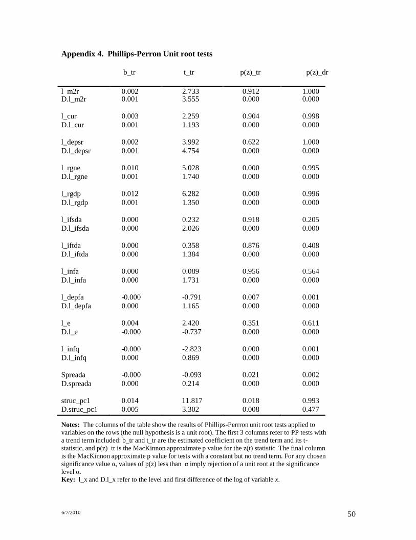
6/7/2010 50

Appendix 4. Phillips-Perron Unit root tests

b_tr t_tr p(z)_tr p(z)_dr

l m2r 0.002 2.733 0.912 1.000 D.l_m2r 0.001 3.555 0.000 0.000

l_cur

0.003

2.259

0.904

0.998 D.l_cur 0.001 1.193 0.000 0.000

l_depsr

0.002

3.992

0.622

1.000 D.l_depsr 0.001 4.754 0.000 0.000

l_rgne

0.010

5.028

0.000

0.995 D.l_rgne 0.001 1.740 0.000 0.000

l_rgdp

0.012

6.282

0.000

0.996 D.l_rgdp 0.001 1.350 0.000 0.000

l_ifsda

0.000

0.232

0.918

0.205 D.l_ifsda 0.000 2.026 0.000 0.000

l_iftda

0.000

0.358

0.876

0.408 D.l_iftda 0.000 1.384 0.000 0.000

l_infa

0.000

0.089

0.956

0.564 D.l_infa 0.000 1.731 0.000 0.000

l_depfa

-0.000

-0.791

0.007

0.001 D.l_depfa 0.000 1.165 0.000 0.000

l_e

0.004

2.420

0.351

0.611 D.l_e -0.000 -0.737 0.000 0.000

l_infq

-0.000

-2.823

0.000

0.001 D.l_infq 0.000 0.869 0.000 0.000

Spreada

-0.000

-0.093

0.021

0.002 D.spreada 0.000 0.214 0.000 0.000

struc_pc1

0.014

11.817

0.018

0.993 D.struc_pc1 0.005 3.302 0.008 0.477

Notes: The columns of the table show the results of Phillips-Perrron unit root tests applied to variables on the rows (the null hypothesis is a unit root). The first 3 columns refer to PP tests with a trend term included: b_tr and t_tr are the estimated coefficient on the trend term and its t- statistic, and p(z)_tr is the MacKinnon approximate p value for the z(t) statistic. The final column is the MacKinnon approximate p value for tests with a constant but no trend term. For any chosen significance value α, values of p(z) less than α imply rejection of a unit root at the significance level α. Key: l_x and D.l_x refer to the level and first difference of the log of variable x.