University of Neuchatel

Institute of Economic Research

IRENE, Working paper 16-04

The Demand for Tap Water Quality:

Survey Evidence on Water Hardness

and Aesthetic Quality Bruno Lanz* Allan Provins**

* University of Neuchâtel (Institute of Economic Research), ETH Zurich (Chair for Integrative Risk Management and Economics), Massachusetts Institute of Technology (Joint Program on the Science and Policy of Global Change).

** Economics for the Environment Consultancy (eftec), London UK.

The demand for tap water quality:

Survey evidence on water hardness and aesthetic quality ∗

Bruno Lanz† Allan Provins‡

This version: September 2016

Abstract

We design a survey to provide quantitative evidence about household demand for quali-

tative aspects of tap water supply. We focus on two characteristics that are of importance

for households: water hardness and aesthetic quality in terms of taste, smell and appear-

ance. Our survey elicits expenditures on products that improve the overall experience

of these characteristics of tap water quality, and administration targets a representative

sample of the population in England and Wales. For water hardness, our results show

that around 14% of households employ at least one water softener device or purchase

products such as softening tablets or descaling agents. For the aesthetic quality of tap

water, around 39% of households report some averting behaviour, the most common be-

ing the use of filtering devices, purchase of bottled water, or addition of squash or cordial.

To study how expenditures on these products vary with the level of service quality, we

match household data to highly disaggregated records on regional water hardness (in

mg CaCO3/l) and aesthetic quality, as measured by the regional rate of complaints to

the water service supplier. Our econometric analysis suggests that households’ decision

to incur averting expenditures varies with service quality in a statistically and econom-

ically significant manner, providing novel evidence that households actively respond to

non-health related aspects of tap water quality.

Keywords: Water demand; Tap water quality; Water hardness; Revealed preferences;

Averting behaviour; Cost-benefit analysis; Economic surveys.

JEL Codes: Q25, Q53, C83, L95, D13.

∗We would like to thank Ian Bateman, Diane Dupont, Scott Reid, seminar participants at the Ecole Polytech-nique Fédérale de Lausanne and the World Conference on Environmental and Resource Economics in Istanbul forhelpful discussions on this work. Comments by two anonymous referees have also led to significant improvementsof the present paper. Excellent research assistance was provided by Martin Baker and Lawrie Harper-Simmonds.The research presented in this paper is based on a study undertaken for a collaborative group of water companies,and we thank the participating companies for allowing us to access their data. The views expressed in this paperand any remaining errors are those of the authors alone.†Corresponding author. University of Neuchâtel, Department of Economics and Business, Switzerland; Chair

for Integrative Risk Management and Economics, ETH Zurich; Joint Program on the Science and Policy of GlobalChange, Massachusetts Institute of Technology. Mail: A.-L. Breguet 2, CH-2000 Neuchâtel, Switzerland; Tel: +4132 718 14 02; email: bruno.lanz@unine.ch.‡Economics for the Environment Consultancy (eftec), London UK.

1 Introduction

The regional monopoly and regulated price control structure of the water sector in England

and Wales means it is not possible to directly observe consumers’ preferences for the specific

components of the services they receive. These aspects of service provision include, for exam-

ple, the reliability of water supply, the frequency of hosepipe bans, and the aesthetic quality

of tap water in terms of taste, smell and appearance. Because the regulatory framework

requires water utilities to periodically produce business plans that reflect consumer prefer-

ences for maintaining and improving service levels, this presents a challenge. Consequently,

the past decade has seen the widespread application of stated preference methods to elicit

consumer preferences and support investment planning with the application of cost-benefit

analysis (e.g. Willis et al., 2005; Lanz and Provins, 2015).

There are, however, also opportunities to apply revealed preference methods, exploiting

consumption decisions for marketed products to infer consumers’ preferences for related non-

marketed goods (see Young, 2005). This includes cases in which products are purchased in

response to insufficient quality of certain aspects of household water supply. Loosely speak-

ing, the averting behaviour or defensive expenditure method suggests that variation in private

expenditures associated with changes in service quality provide evidence about the demand

for service quality (e.g. Courant and Porter, 1981; Smith and Desvousges, 1986; Smith, 1991;

Dickie, 2003).1 For instance, consumers can respond to service failures such as unpleasant

taste or smell of tap water by purchasing products such as water filters and bottled water.

These products are assumed to be purchased so long as the value of the disamenity that is

avoided is larger than the marginal expenditure on these products. Importantly, it is implied

that if the quality of tap water was adequate, consumers would not make averting expendi-

tures. Therefore, in this model an improvement in service quality is associated with a reduc-

1 The theoretical foundation for the averting behaviour approach is based on the canonical model of householdproduction, in which households combine commodities purchased on the market with other inputs (notablynon-market amenities and their time) to produce goods that they value for consumption (Becker, 1965;Grossman, 1972). When incurring averting expenditures, households trade-off the disamenity of under-provision of a public good with the costs of investments to protect themselves against under-provision. Inthe context we consider, households may select their preferred level of service by combining the quality ofwater at the tap with market goods that are either complements (such as filters) or substitute products (suchas bottled water).

1

tion in averting behaviour and therefore lower expenditures on substitute and complement

products.

In this paper we design a household survey focusing on averting behaviour for two specific

characteristics of tap water supply, namely water hardness and aesthetic quality in terms of

taste, smell and appearance. Hard water (via scaling) can damage and significantly reduce

the lifetime of water-using appliances, implying notable costs to households. Whilst the level

of hardness is a characteristic of the raw water source and is determined by the geology of

the area from which water is abstracted (specifically the presence of calcium and magnesium

in aquifers), it can be mitigated by investments by the water company in treatment plants

or at the individual household level.2 In addition, the aesthetic characteristics of tap water

are important to consumers, and this dimension of service provision is directly related to

investments by utility companies (e.g. the frequency of cleaning of water mains or their

replacement).

The survey, which was administered in England and Wales, covers a wide geographical

area supplied by different water services suppliers. It elicits detailed information on house-

holds’ perceptions of tap water quality, the type of products purchased in relation to water

hardness and aesthetic quality of tap water, and the motivations for doing so. Results from

the survey on households’ attitudes, motivations and behaviour provide clear evidence that

consumers do purchase market goods in response to qualitative aspects of tap water. For wa-

ter hardness, around 14% of respondents report some form averting behaviour. For aesthetic

quality, almost 40% of respondents relate their use of marketed products to issues concerning

the quality of tap water, although average annual expenditures per household are lower than

for water hardness.

Survey responses are augmented with detailed data on regional tap water quality, which

is sourced from company reporting to the Drinking Water Inspectorate (DWI) for England

and Wales,3 and includes physical data on average water hardness and the rate of customer

2 However, while it is possible to reduce water hardness during the treatment process, water companies inEngland and Wales do not currently do this.

3 This data refers to water supply zone (WSZ), which are geographical areas in which water supply is from thesame source(s), so that quality can be assumed to be the same for all households within the same zone.

2

complaints to water service suppliers in relation to the taste, smell and appearance of tap

water. This rich set of data enables us to explore whether averting expenditures vary system-

atically with the local level of service provision, as well as relevant households’ characteris-

tics.4 Variation in averting expenditures are modelled with a Tobit model (Tobin, 1958), an

approach which is standard in the literature (e.g. Um et al., 2002), as well as a more flexible

alternative suggested by Cragg (1971). The latter model allows separate consideration of

the (binary) decision to incur averting expenditures and, conditional on observing positive

averting expenditures, the level of expenditures.

Our results provide evidence that households’ averting behaviours respond to our mea-

sure of objective service quality, which is in line with standard applications of the method in

the context of health risks (see for example Gerking and Stanley, 1986, and Deschenes et al.,

2012, on air quality, and Zivin et al., 2011, on water pollution).5 Quantitatively, we find that,

at the mean of the sample, a 10% reduction in water hardness (measured in mg of calcium

carbonate, CaCO3) is associated with a GBP 1.00 – 1.30 reduction in yearly averting expen-

ditures depending on the model used to analyse the data. With respect to aesthetic quality,

we find that averting behaviour is mainly driven by the taste and smell of tap water rather

than issues with its appearance. At the mean of the sample, a one point reduction in the

number of taste/smell complaints per thousand of customers is associated with a GBP 13.31

– 15.95 reduction in averting expenditures, again depending on the model used. Therefore,

overall, we find that households purchase market products as a response to non-health risk

related aspects of tap water quality, and do so in an economically significant manner.

4 Note that customer complaint data provides a convenient measure of relative performance of suppliers andis readily collected by all water utilities in England and Wales. It therefore provides a policy-relevant startingpoint to use in conjunction with averting expenditures, although we acknowledge that it is not an idealmeasure of service quality.

5 Because objective quality only affects behaviour through perception, some authors relate averting expendi-tures to subjective rating (or quality perception); see Abrahams et al. (2000) for an application to waterhealth risks. Such an approach is, however, problematic because replacing objective service provision withsubjective perception makes marginal benefits difficult to interpret when assessing the socially optimal pro-vision of public goods. Moreover, as initially noted by Whitehead (2006), there is a potential endogeneityissue associated with the use of self-reported rating (see also Adamowicz et al., 2014; Bontemps and Nauges,2016). In a companion paper, Lanz and Provins (2016), we contribute to this literature by proposing ageneral solution to the use of perceived quality, and we illustrate our approach with data derived from oursurvey. In the present paper, the econometric analysis rather focuses on providing evidence about the internalvalidity of responses to our survey instrument, using a more standard model relating averting expendituresto objective quality.

3

The quantitative evidence derived from our survey is novel from at least two perspec-

tives. First, whereas a large literature has focused on failures in relation to tap water quality

standards and risks to human health (Abdalla et al., 1992; Larson and Gnedenko, 1999; Abra-

hams et al., 2000; McConnell and Rosado, 2000; Yoo and Yang, 2000; Wu and Huang, 2001;

Um et al., 2002; Rosado et al., 2006; Lee and Kwak, 2007; Jakus et al., 2009; Zivin et al.,

2011; Dupont and Jahan, 2012), we study averting behaviour in a context where risks to

human health are negligible.6 Therefore, to the best of our knowledge, our survey provides

the first quantitative evidence on the demand for non-health dimensions of tap water quality.

Because improving tap water services requires costly and long-lived investments, quantitative

evidence about such preferences is of importance for most developed countries (Whittington

and Hanemann, 2006). Second, our survey work represents the first application of a revealed

preference approach in the context of water service regulation in the UK. On the one hand,

our survey data provide quantitative evidence about the economic benefits associated with

service improvements, which can be compared against investment costs to improve the level

of services. On the other hand, as we discuss in more detail below, our results provide an

interesting counter-point to the challenges raised by the widespread use of stated preference

methods, notably discrete-choice experiments (see e.g. Ofwat, 2016a,b).

The remainder of the paper proceeds as follows. In Section 2 we present the details of our

survey instrument. Section 3 describes the main results from the administration of our survey,

including spatial coverage of the sample, a summary of the extent of averting behaviour by

sampled households, and pairwise correlations between averting behaviour, service ratings,

and our measures of objective service quality. Section 4 reports the econometric analysis of

averting expenditures in relation to objective service provision. Section 5 discusses our results

in the context of the wider regulatory environment in England and Wales, and provides some

concluding comments.

6 In England and Wales, compliance with UK and European drinking water standards across 39 parameters was99.96% in 2012 (DWI, 2013). Note however that perceived health risks associated with tap water consump-tion (which, for example, could be triggered by aesthetic quality issues) may motivate averting behaviour.

4

2 Description of the survey instrument

The development of the survey material proceeded in two phases. First, questions on house-

holds’ consumption of tap water and extent of averting behaviour in relation to water hard-

ness and aesthetic quality of tap water were trialled in a national omnibus survey. Based on

a sample size of approximately 2,000 respondents, results indicated that alternatives such

as bottled water and filtering tap water represented averting behaviours for approximately

20 to 30 percent of households. In the second step the survey instrument was tested via an

online pilot with a sample of approximately 200 respondents.

The structure of the final survey features several sections, starting with a screening ques-

tion on respondents’ responsibility for paying the household’s water bills.7 Respondents who

are screened-in are asked a number of warm-up questions to record the number of people

in the household and their age, as well as their consumption of tap water both for drinking

and for other uses. We then ask about potential averting behaviours, such as the use of a

jug/kettle with filter, tap/under sink filter, bottled water, squash and cordial, as well as water

softener appliances and products such as softening tablets. Respondents who indicate the

use of a specific product are directed to follow-up questions on their uses of these products

(e.g. drinking, food preparation, etc.), associated expenditures (both one-off and recurring

amounts), and frequency of purchases. In order to ascertain whether these purchases rep-

resent an averting behaviour, we ask about their motivations for the purchases, including

reasons related to concerns about the taste, smell and colour of tap water, health concerns,

advice from third parties (water companies, medical professionals, media, advertising, etc.),

and other potential factors such as convenience.

We then ask follow-up questions about experiences of tap water, including problems with

the taste, smell and colour of tap water (including chlorine or musty taste, cloudy appear-

ance, sediment, brown/orange colouring, etc.), perceptions regarding its quality (e.g. hard-

ness, impurities, mineral content of substitutes, etc.) and health risks (e.g. risk of illness,

contaminants and pollutants, lead in supply pipes, the addition of fluoride, chemicals used to

7 A copy of the final survey was made available for the peer-review process, and can be obtained from theauthors upon request.

5

treat drinking water, etc.), as well as advice received about consumption of tap water from

a water company (e.g. ‘boil water’ notices, ‘do not drink’ notices). We then elicit the re-

spondent’s ratings of the tap water supply at their home in several dimensions: taste, smell,

appearance, hardness, and overall quality. The survey concludes with background questions

about the respondent household, including how long they have lived at their current ad-

dress, their previous place of residence, whether they have a water meter, their annual water

services bill amount, as well as questions about the health status of all members of the house-

hold.

We administered the survey through an online market-research platform providing us

access to a panel of over 300,000 individuals, which is designed to facilitate nationally rep-

resentative fieldwork. This allows us to draw a representative sample by setting up quotas

on a number of key characteristics of the respondents, namely age, gender, and social class.

The survey was administered in November and December 2012, and potential participants

were contacted by drawing a random sample of panel members (conditional on the quotas)

with the following email message: “We are conducting a survey on water services and tap

water. If you would like to take part please click this link.” The response rate to our invitation

was around 1 in 6, and, by construction, the quotas imply that our sample is broadly rep-

resentative of the population of England and Wales.8 Our sampling procedure also exploits

information about the location of respondents. Specifically, a geographically representative

sample of 1,000 respondents was targeted for England and Wales, and a further 3,500 re-

spondents were sampled from within the supply areas of seven water services suppliers in

England and Wales (approximately 500 respondents per company).9 This was to enable

company-specific results to be estimated for these suppliers. For the econometric analysis,

we employ weights to obtain results that are representative of the population of England and

Wales.

8 We acknowledge that there is a potential for sample selection, with households dissatisfied with their waterservices potentially more likely to participate in the survey. However, the generality of the invitation messageshould mitigate any bias specific to water hardness and aesthetic quality issues.

9 A total of nine water service suppliers in England and Wales participated in the study. For seven companies,an additional sample of 500 respondents was targeted. Note that the nationally representative sample ofapproximately 1,000 households also includes respondents from other water service suppliers.

6

In order to support the analysis of household’s averting behaviour, data resulting from

survey administration are augmented by a range of data on local tap water quality and hard-

ness service levels. This data mainly allows us to study how averting behaviour elicited with

the survey varies with the level of service provided across different areas. The data refers to

highly disaggregated WSZs, for which we can assume that source water quality is the same

as water supplied is typically from a single treatment works. For each WSZ, we have data on

water hardness expressed as mg CaCO3/l, the number of customer contacts (complaints)

relating to taste/smell of tap water, and its appearance, and the population within the WSZ.

We match survey respondents to their WSZ through their home postcode.

3 Descriptive results from the survey

A total of 4,520 households were sampled via the online survey. This comprised of 1,056

respondents in the nationally representative ‘base’ sample, and a further 3,464 households

in the combined company-specific sample. The geographical composition of the sample is

reported in Figure 1. Summary statistics for socio-demographic characteristics are provided

in Appendix A.

Table 1 reports average household ratings for hardness, taste, smell, and appearance of

tap water from the overall pooled sample and individual company areas. The majority of

households (74%) rated their tap water overall to be in the range ‘adequate’ – ‘good’ on

a 5-part Likert scale. For the aesthetic quality of tap water, both the pooled sample average

and individual companies subsamples show that appearance of tap water receives the highest

rating, followed by its smell and then taste. Moreover, households’ perception of aesthetic

quality does not vary significantly across companies, there is substantial variation in the

rating of water hardness.

Averting behaviour by households is summarised in Table 2 across the overall pooled

sample (N=4,520). Starting with water hardness, just over 1 in 10 respondents report some

form of defensive or mitigating actions; the most common being the use of water softener

products for washing machines, dishwashers and kettles. Averting behaviour in relation to

aesthetic quality is more prevalent, as almost 4 in 10 households report some form of averting

7

Figure 1: Spatial composition of the sample, England and Wales

action. The most common averting behaviour is the use of a jug with a filter (18.4%) followed

by the purchase of bottled water (16.3%).

Results reported in Table 2 exploit responses to the follow-up questions in order to identify

relevant averting behaviour and expenditures. In particular, only 1 in 3 households cite

8

Table 1: Household rating of tap water – water hardness and aesthetic quality

Hardnessa Tasteb Smellb Appearanceb

Overall pooled sample 3.4 3.6 3.7 4.0Company 1 2.4 3.8 3.9 4.2Company 2 4.2 3.5 3.7 3.9Company 3 4.0 3.5 3.7 4.0Company 4 4.2 3.4 3.6 3.9Company 5 2.5 3.7 3.7 4.1Company 6 4.0 3.5 3.7 4.0Company 7 2.2 3.5 3.7 4.0

Notes: Pooled sample includes all observations (N = 4,520). Individual company samples: N between487 and 503. aRatings for hardness are based on the scale ‘very soft’ (=1), ‘soft’ (=2), ‘medium’ (=3),‘hard’ (=4), and ‘very hard’ (=5). bRatings for taste, smell and appearance of tap water are based onthe scale: ‘bad’ (=1); ‘poor’ (=2); ‘adequate’ (=3); ‘good’ (=4); and ‘excellent’ (=5).

deficient aesthetic quality as the main reason for undertaking the reported actions. Dislike

of the taste and smell of tap water (27%) is the most frequent response, while dislike of

the appearance of tap water is cited as a motivation by relatively few households (5%), and

ranked lower in considerations than the temperature of tap water (7%), for example. The

second most common motivation is the convenience of bottled water, with 1 in 4 respondents

stating this as being a reason for their behaviour (the re-use of bottles was stated by 12% of

respondents). Following this, respondents who reported that their purchases of bottled water

were solely due to convenience factors or the re-use of bottles are not included in the analysis

of averting behaviour.

A key motivation for averting behaviour is found to be the perception of the quality of

marketed products, which is split between a general view that they are better quality than

tap water (23%) or that they are healthier than tap water (about 18%). Relatively few

respondents stated that these products represented ‘value for money’ (6%), but a greater

number stated that their purchases and/or actions were formed largely out of habit (13%).

Finally less than 2% of respondents stated that advice not to drink tap water had influenced

their use of marketed products.

Turning to our results for averting expenditures, we first note that a small fraction of

9

Table 2: Averting behaviour – water hardness and aesthetic quality

Averting behaviour Averting expenditures% respondents % respondents Mean (GBP/yr) Median (GBP/yr)

Water hardness

Water softener device (total) 5.1 3.5 149.5 60.0Ion exchange unita 3.0 2.0 233.5 160.0Chemical conditioning unita 0.8 0.4 77.7 37.5Physical conditioning unita 1.5 1.1 18.7 15.0

Water softener products (total) 9.9 9.7 66.3 48.0Tablets/powder 8.1 7.9 51.6 36.0Kettle descaler 4.9 4.5 24.7 12.0Limescale remover 4.5 4.3 28.7 24.0

TOTALc 13.9 12.1 94.4 50.0

Aesthetic quality

Filtering devices (total) 26.0 21.6 71.0 40.0Jug with filtera 18.4 16.9 60.4 39.0Kettle with filtera 2.8 2.4 63.9 25.0Tap/under-sink filtera 4.0 3.4 75.8 50.0Fridge with dispensera,b 2.8 1.9 134.9 107.5Water dispenser/purifiera 1.0 0.8 138.2 69.5Other filtering appliancesa 0.2 0.2 44.6 38.0

Bottled water 16.3 11.0 87.9 60.0Purification tablets 0.4 0.3 55.7 42.0Cordial/squash 7.3 6.1 59.3 48.0

TOTALc 38.7 27.6 91.7 60.0

Notes: Table reports averting behaviour and expenditures for the pooled sample (N = 4,520). Thefirst column reports the proportion of respondents who engage in averting behaviour, the secondcolumn is the proportion of respondent who report positive averting expenditures. The differencebetween the first two columns reflect the share of respondents who were not able to report amountsspent on specific products. The third and fourth columns report mean and median expenditures,respectively, for those respondents with positive averting expenditures. aDenotes assumption thatcapital expenditures are annualised over a five year period; bOnly a fraction of the one-off purchasecost potentially represents averting behaviour hence expenditure on fridges with dispenser is excludedfrom the calculation of total annual average expenditure. cTotal figures account for multiple avertingbehaviours by the respondents, including annualised one-off purchase amounts.

respondents who reported averting behaviour were not able to state the associated expen-

ditures. This is shown as the difference between the first and second columns of Table 2.

These respondents are excluded from the analysis focusing on expenditures. For respondents

who report positive averting expenditures related to water hardness (N=547), we observe

that these households spend on average approximately GBP 94 per year in response to hard-

10

Figure 2: Distribution of households’ annual averting expenditures0

5010

015

0Fr

eque

ncy

(num

ber o

f res

pond

ents

)

0 200 400 600 800Positive averting expenditures: Water hardness (£/household/year), N=547

010

020

030

0Fr

eque

ncy

(num

ber o

f res

pond

ents

)

0 100 200 300 400 500Positive averting expenditures: Taste, smell and appearance (£/household/year), N=1248

ness of tap water, with a median value of GBP 50 per household per year.10 For respondents

with positive expenditures related to aesthetic quality of tap water (N=1,248), average an-

nual averting expenditure is approximately GBP 92 per household per year, while the median

value is GBP 60 per household per year. The distribution of annual household averting ex-

penditure is presented in Figure 2 for hardness and aesthetic quality. Notice that, while

the proportion of households with aesthetic quality related expenditures is greater than the

proportion for water hardness, individual amounts are smaller.

Table 3 reports pairwise (polyserial) correlation coefficients for respondents’ tap water

quality ratings and averting behaviour related to the hardness of tap water. It shows that

respondents who rate their tap water to be ‘hard’ are more likely to undertake averting actions

related to hardness of tap water. Moreover, we observe that respondent hardness rating is

strongly correlated to average water hardness (mg CaCO3/l) in the relevant WSZ. This

suggests that the respondents have well-formed perceptions of water hardness, an important

pre-requisite for applying the averting behaviour method.

Turning to the aesthetic quality of tap water, Table 4 reports (polyserial) correlation coef-

10 This represents the sum of all averting expenditures across all products, where capital outlays are spreadequally over a 5 year period, which was found to be the typical life span for appliances considered. Capitalexpenditures could be annualised using alternative assumptions, although implications for the results areminor.

11

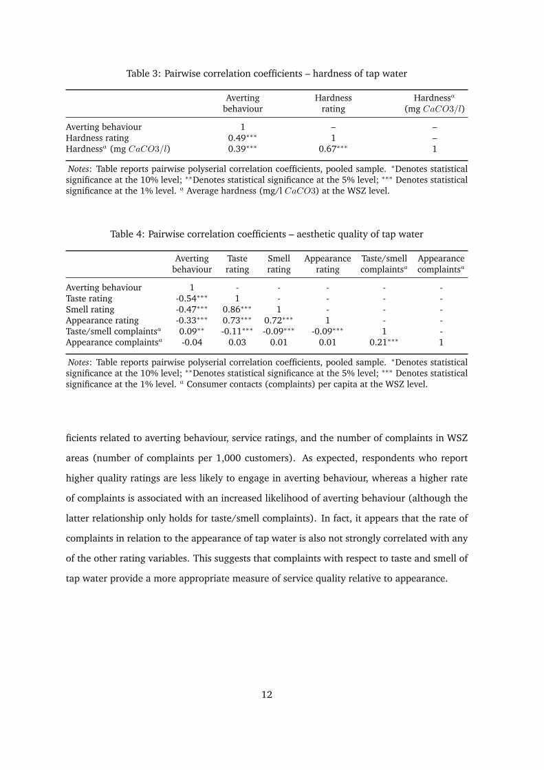
Table 3: Pairwise correlation coefficients – hardness of tap water

Averting Hardness Hardnessa

behaviour rating (mg CaCO3/l)

Averting behaviour 1 – –Hardness rating 0.49∗∗∗ 1 –Hardnessa (mg CaCO3/l) 0.39∗∗∗ 0.67∗∗∗ 1

Notes: Table reports pairwise polyserial correlation coefficients, pooled sample. ∗Denotes statisticalsignificance at the 10% level; ∗∗Denotes statistical significance at the 5% level; ∗∗∗ Denotes statisticalsignificance at the 1% level. a Average hardness (mg/l CaCO3) at the WSZ level.

Table 4: Pairwise correlation coefficients – aesthetic quality of tap water

Averting Taste Smell Appearance Taste/smell Appearancebehaviour rating rating rating complaintsa complaintsa

Averting behaviour 1 - - - - -Taste rating -0.54∗∗∗ 1 - - - -Smell rating -0.47∗∗∗ 0.86∗∗∗ 1 - - -Appearance rating -0.33∗∗∗ 0.73∗∗∗ 0.72∗∗∗ 1 - -Taste/smell complaintsa 0.09∗∗ -0.11∗∗∗ -0.09∗∗∗ -0.09∗∗∗ 1 -Appearance complaintsa -0.04 0.03 0.01 0.01 0.21∗∗∗ 1

Notes: Table reports pairwise polyserial correlation coefficients, pooled sample. ∗Denotes statisticalsignificance at the 10% level; ∗∗Denotes statistical significance at the 5% level; ∗∗∗ Denotes statisticalsignificance at the 1% level. a Consumer contacts (complaints) per capita at the WSZ level.

ficients related to averting behaviour, service ratings, and the number of complaints in WSZ

areas (number of complaints per 1,000 customers). As expected, respondents who report

higher quality ratings are less likely to engage in averting behaviour, whereas a higher rate

of complaints is associated with an increased likelihood of averting behaviour (although the

latter relationship only holds for taste/smell complaints). In fact, it appears that the rate of

complaints in relation to the appearance of tap water is also not strongly correlated with any

of the other rating variables. This suggests that complaints with respect to taste and smell of

tap water provide a more appropriate measure of service quality relative to appearance.

12

4 Econometric analysis of averting expenditures

The main objective of our econometric analysis is to provide evidence about the internal va-

lidity of responses to our survey instrument, quantifying the relationship between averting

expenditures and the level of service provision. Relating variation in an objective measure of

service provision to the observed level of averting expenditures represents a standard applica-

tion of the averting behaviour method (see e.g. Deschenes et al., 2012, and other papers cited

in the introduction). The marginal effect of service quality on averting expenditures provides

a measure of the marginal benefit, from the perspective of a representative household, of

an improvement in the level of service. In addition, our analysis controls for a number of

households’ characteristics that might influence averting behaviours, such as socio-economic

(e.g. household income), demographic (e.g. household composition), and other contextual

factors (e.g. the length of residence in the current dwelling).

The dependent variable in the regression analysis is total averting expenditures (i.e. ex-

penditures on products improving water hardness and aesthetic quality that are explicitly

related to service failures).11 We treat averting expenditures as a corner solution outcome,

and use both a Tobit model (Tobin, 1958) and Craggs’ (1971) two-tier model to represent

the conditional expectation of expenditures. Importantly, the two models share the same

underlying distributional assumptions, although they differ in that the Cragg model allows

the processes determining the probability of positive averting expenditure and the amount

observed (when larger than zero) to be driven by different determinants. Note that the Cragg

model reduces to the Tobit model when the parameters of the two processes are constrained

to be the same.12

The key covariate in the regression analysis is the measure of the level of service, i.e.

11 For each individual, we sum expenditures across all product categories reported in Table 2. As noted pre-viously, capital expenditures are annualised over a five year period, and for recurring expenditures we useinformation from the respondents as to the frequency of purchases within a year. Respondents who did notreport averting expenditures are excluded form the analysis, and we also exclude expenditures on fridgeswith a water dispenser.

12 Formally, the Tobit model is nested in the Cragg model, and the latter combines a probit model for thebinary decision to incur averting expenditures or not, and a truncated normal regression to model positiveexpenditures. See Wooldridge (2010, p. 692). Marginal effects in the Cragg model are derived using theStata command by Burke (2009).

13

the quality of tap water. In the present setting, our measure of objective service provision is

average water hardness measured in mg CaCO3 per litre and the rate of complaints related

to taste / smell and appearance (the number of complaints per thousand of customers). In

the following analysis, we therefore assume that these two measures of service can be taken

as exogenous.13 First, it is highly unlikely that these water services characteristics enter

household’s location decisions, which rules out spatial sorting and associated endogeneity of

objective provision. Second, tap water quality regulation in England and Wales enforces strict

compliance with European drinking water standards (see DWI, 2013), and information about

WRZ boundaries and characteristics of associated treatment plants are typically not known

by households. This makes an association between the service level for non-risk related fea-

tures of water supply and local socio-economic outcomes very unlikely. Finally, the measures

we consider are relevant from the perspective of regulation and resource management, and

since they correlate with self-reported rating variables (see Table 3 and 4) they are taken as

good candidates to assess consistency of our averting expenditure data within the averting

behaviour model.

Estimation results for averting expenditure in response to the hardness of tap water are

presented in Table 5. Specification I is the standard Tobit model, for which we report both

the parameter estimates and marginal effects evaluated at the mean of the sample. Specifica-

tion II is the Cragg two-tier model, for which we report parameter estimates for the selection

equation (a probit model where the dependent variable is equal to one when averting ex-

penditure are positive, zero otherwise), and a truncated normal model (explaining the level

of expenditures when these are greater than zero). We further report marginal effects asso-

ciated with each variable, evaluated at the mean of the sample. For both the Tobit model

and the Cragg model, marginal effects account for both the effect of each covariate on the

probability of positive expenditures and on the amount spent. Therefore, marginal effects

computed from the Tobit and Cragg models are consistent and can meaningfully be com-

pared. For both models we also include a set of households characteristics to control for key

13 The exogeneity of our measures of objective provision is discussed extensively in Lanz and Provins (2016).

14

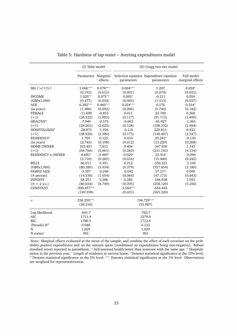
Table 5: Hardness of tap water – Averting expenditures model

(I) Tobit model (II) Cragg two-tier model

Parameters Marginal Selection equation Expenditure equation Full modeleffects parameters parameters marginal effects

MG CaCO3/l 1.066∗∗∗ 0.078∗∗∗ 0.004∗∗∗ 1.207 0.059∗

(0.192) (0.015) (0.001) (0.874) (0.031)INCOME 1.025∗∗ 0.075∗∗ 0.005∗ -0.211 0.054(GBPx1,000) (0.477) (0.034) (0.003) (1.213) (0.037)AGE 6.282∗∗∗ 0.460∗∗∗ 0.024∗∗∗ 6.576 0.334∗

(in years) (1.486) (0.092) (0.006) (5.740) (0.182)FEMALE -11.698 -0.853 0.011 23.740 0.360(=1) (26.522) (1.902) (0.117) (91.713) (1.499)HEALTHYa -7.949 -0.575 -0.063 -65.927 -1.365(=1) (28.201) (2.025) (0.128) (108.332) (1.984)HOSPITALISEDb -28.873 -1.926 -0.110 220.811 0.922(=1) (38.920) (2.380) (0.175) (148.407) (2.347)RESIDENCYc 1.705 0.125 0.010 -25.241∗ -0.130(in years) (2.743) (0.198) (0.012) (13.229) (0.208)HOME OWNER 103.851 7.812 0.404 -347.930 1.143(=1) (64.766) (5.061) (0.283) (231.163) (4.134)RESIDENCY x OWNER -6.681∗ -0.489∗ -0.029∗ 23.916 -0.096

(3.716) (0.265) (0.016) (15.440) (0.242)BILLS 60.011 4.391 0.212 -356.321 -1.104(GBPx1,000) (80.389) (5.934) (0.379) (357.654) (5.180)FAMILY SIZE -3.397 -0.249 -0.042 57.217 0.090(# person) (14.336) (1.054) (0.064) (47.173) (0.843)INFANTS 58.251 5.286 0.285 -166.038 1.592(# < 2 y.o.) (80.034) (8.749) (0.395) (258.129) (5.256)CONSTANT -900.457∗∗∗ -3.564∗∗∗ -654.443

(149.598) (0.431) (565.320)

σ 238.250∗∗∗ 196.729∗∗∗

(28.216) (52.987)

Log-likelihood -841.7 -762.7AIC 1711.4 1579.0BIC 1780.5 1712.6(Pseudo) R2 0.048 0.123N 1,029 1,029N corner 901 901

Notes: Marginal effects evaluated at the mean of the sample, and combine the effect of each covariate on the prob-ability positive expenditures and on the amount spent (conditional on expenditures being non-negative). Robuststandard errors reported in parenthesis. a Self-assessed health better than someone with the same age. b Hospitali-sation in the previous year. c Length of residence at current home. ∗Denotes statistical significance at the 10% level;∗∗Denotes statistical significance at the 5% level; ∗∗∗ Denotes statistical significance at the 1% level. Observationsare weighted for representativeness.

15

potential determinants of averting expenditures.14

Estimates from Specification I indicate that averting expenditures are positively related

to the measure of water hardness and household income. This is important as it provides

confidence that the results from the survey conforms with prior expectations. Specifica-

tion II further reveals that these two variables mainly influence the decision of whether or

not to incur averting expenditures, rather than the amount spent, as signified by statistical

(in)significance of the respective parameters in the expenditure equation. Note, however,

that the sample of respondents with positive averting expenditures, on which the expendi-

ture equation is estimated, is relatively small (N=128), which penalises the precision of our

estimates. We also find that most of the socio-demographic determinants included in the anal-

ysis are not statistically significant, which demonstrates that there is significant unobserved

heterogeneity. Respondent age is an exception, with older respondents being more likely to

report positive expenditures in relation to water hardness than younger respondents. This

is possibly due to greater experience of the effect of hard water on the lifetime of consumer

appliances.

We also note that goodness-of-fit measures favour the more flexible two-tier specification,

even when penalised for the fact that the number of estimated coefficient is almost two

times larger (i.e. the BIC is lower in Specification II). Our measure of the marginal benefit

associated with a reduction of water hardness is very similar across the two specifications. At

the mean of the sample, a reduction of water hardness by 1 mg CaCO3 per litre is associated

with a reduction in averting expenditures by around GBP 0.08 per household per year for the

Tobit model, and GBP 0.06 in Cragg’s two-tier model.

Econometric results for averting expenditures in relation to the aesthetic quality of tap

water are presented in Table 6. As for water hardness, specification I is a standard Tobit

model, for which we report both parameter estimates and marginal effects evaluated at the

mean of the sample. Specification II is the Cragg model, for which we report coefficient es-

14 Note that the sample size is lower than the total pooled sample, as respondents who did not indicate theirhousehold income and averting expenditures are excluded from the analysis, and because of missing postcodeinformation precluding the matching of household-level data to regional (WSZ) data. Balance tests acrosssubsamples do not reveal any statistically significant differences in means, suggesting no sample selectionproblems (at least for the household characteristics we observe).

16

Table 6: Aesthetic quality of tap water – Averting expenditure model

(I) Tobit model (II) Cragg two-tier model

Parameters Marginal Selection equation Expenditure equation Full modeleffects parameters parameters marginal effects

COMPLAINTS: 55.223∗∗ 15.947∗∗ 0.451∗∗∗ 3.834 13.312∗

TASTE/SMELL (23.388) (6.713) (0.155) (10.510) (7.298)COMPLAINTS: -4.452 -1.286 -0.030 8.955 -0.493APPEARANCE (2.810) (0.814) (0.021) (12.409) (0.766)INCOME -0.013 -0.004 0.002 0.112 0.057(GBPx1,000) (0.267) (0.077) (0.002) (1.023) (0.060)AGE -0.263 -0.076 0.005 -4.106 -0.035(in years) (0.762) (0.222) (0.004) (3.084) (0.187)FEMALE -38.246∗∗ -11.206∗∗ -0.079 -217.553∗∗ -11.816∗∗

(=1) (15.294) (4.571) (0.089) (85.699) (5.832)HEALTHY -5.420 -1.551 -0.018 49.621 1.636(=1) (16.474) (4.665) (0.093) (70.142) (4.250)HOSPITALISED 38.903∗ 12.776∗ 0.371∗∗∗ 109.973 15.646∗∗

(=1) (20.954) (7.684) (0.136) (94.526) (7.910)RESIDENCY -0.603 -0.174 -0.013 8.318 -0.003(in years) (1.332) (0.385) (0.008) (5.773) (0.358)HOME OWNER 43.471 13.382 -0.023 190.005 7.634(=1) (37.025) (12.160) (0.183) (126.156) (8.072)RESIDENCY x OWNER -0.382 -0.110 0.011 -11.910 -0.199

(1.834) (0.530) (0.010) (7.411) (0.460)BILLS -34.136 -9.858 -0.237 225.853 2.969(GBPx1,000) (45.292) (13.089) (0.287) (203.063) (12.085)FAMILY SIZE 3.894 1.124 -0.023 113.115∗∗ 4.285(# person) (6.979) (2.020) (0.045) (44.168) (2.771)INFANTS -25.951 -6.784 0.179 -401.291 -12.329(# < 2 y.o.) (48.912) (11.531) (0.374) (280.524) (17.362)FEMALE x INFANTS 91.600 36.864 0.301 266.467 20.450

(65.371) (34.164) (0.563) (286.288) (21.769)CONSTANT -66.605 -0.724∗∗∗ -488.292∗∗

(42.468) (0.267) (232.464)

σ 144.174∗∗∗ 196.533∗∗∗

(9.755) (32.529)

Log-likelihood -2436.6 -2398.2AIC 4903.8 4859.4BIC 4983.9 5013.4(Pseudo) R2 0.008 0.023N 1,074 1,074N corner 735 735

Notes: Marginal effects evaluated at the mean of the sample, and combine the effect of each covariate on the prob-ability positive expenditures and on the amount spent (conditional on expenditures being non-negative. Robuststandard errors reported in parenthesis. a Self-assessed health better than someone with the same age. b Hospitali-sation in the previous year. c Length of residence at current home. ∗Denotes statistical significance at the 10% level;∗∗Denotes statistical significance at the 5% level; ∗∗∗ Denotes statistical significance at the 1% level. Observationsare weighted for representativeness.

17

timates associated with both the decision of whether or not to incur averting expenditures

(selection equation) and the level of averting expenditures (expenditure equation). We also

report marginal effects evaluated at the mean of the sample, which combine the impact of

each variable on the probability of positive expenditures and the level of expenditures. As be-

fore, all models include a set of explanatory variables related to households characteristics.15

Specification I indicates a positive association between the rate of complaints for taste and

smell and averting behaviour, but not for complaints concerning the appearance of tap water

(the latter estimate has the wrong sign but is not statistically different from zero). This result

mirrors the correlation patterns reported in Table 4 and is consistent with the observation that

the appearance of tap water has the highest rating among all three aesthetic quality attributes

(see Table 1). As for water hardness, Specification II suggests that the effect of aesthetic

quality mainly occurs through changes in the probability of incurring averting expenditures,

although the sample for the expenditure equation (N=339) is again significantly smaller

than that for the selection equation. This of course affects the precision of estimates in the

expenditure equation. We also find that whether a respondent has been hospitalised in the

year leading up to the study is associated with a higher probability of averting behaviour, but

with little discernible effect on the level of expenditures. However, a key driver of expenditure

is the number of persons living in the household.

Our estimate of the benefit associated with a marginal reduction of the rate of taste and

smell complaints is again consistent across the two models. For the Tobit model, it is around

GBP 16 per household per year, while for the Cragg two-tier model it is slightly above GBP

13 per household per year. Comparing goodness-of-fit statistics, we observe that the AIC

and the pseudo-R2 improve with the more flexible two-tier model, although the BIC (which

penalises for the number of coefficient estimated) suggests otherwise. Therefore, evidence

for preferring one model over the other is ambiguous, and the fact that welfare estimates are

very similar across models is reassuring.

15 The sample size is again smaller than the total pooled sample size, as observations with missing income andaverting expenditures are omitted, and missing postcode information precludes matching households to theirWSZ and associated complaint rate. As for water hardness, this could raise concerns about sample selection,although we do not find statistically significant differences in (observed) households characteristics acrosssubsamples.

18

5 Discussion and conclusion

The survey developed in this paper represents the first application of an averting behaviour

approach to the estimation of the demand for tap water quality in England and Wales. It

quantifies households’ preferences in relation to the hardness and the aesthetic quality of

tap water (taste, smell and appearance). In contrast to previous applications of the averting

behaviour and defensive expenditure approach, which focus on health risks associated with

tap water consumption, we consider qualitative (non-health risk related) aspects of tap wa-

ter supply. In this setting, consumer behaviour is driven by preferences for tap water quality,

along with a host of other lifestyle and convenience factors. Evidence from our large-scale

national survey eliciting complementary information on households’ motivations for their

averting behaviours suggests that household’s experience of hard water and aesthetic qual-

ity is a key determinant of decisions to purchase and use averting products. Although our

estimated models do not account for a significant part of the variance of observed avert-

ing expenditures, our analysis confirms that averting behaviour does vary with the level of

service.

From a water sector investment planning perspective, results from our survey provide evi-

dence about the benefit to household consumers of improved levels of service. The regulatory

framework in England and Wales requires that water utilities develop business plans that de-

liver the greatest benefit for customers subject to several constraints, including the cost of

maintaining and improving services, and the affordability of overall bills. Information on

household preferences and the demand for improved service levels is therefore an important

input to the development of business plans in order to understand the ’value for money’ of

potential investments and service improvements. Indeed cost-benefit analysis principles un-

derlie the investment modelling and optimisation processes that shape company’s business

plans (see for example UKWIR, 2010).16

Our study also provides a counter-point to the application of stated preference studies in

16 Anecdotally, the cost of reducing water hardness at the treatment plant level is typically very high; howeverunit cost estimates for reducing water hardness are not publicly available and are confidential information inthe context of the regulatory price control process. Hence it is not possible to provide an indicative view onhow our marginal benefit estimates compare to indicative marginal costs of investment for water utilities.

19

water sector in the UK. Whilst the results detailed here should not be interpreted as ‘bench-

marks’ against which stated preference values should be assessed, they do provide a basis

for judging how expressed preferences for improved tap water quality align with observed

consumer behaviour in relation to marketed products (e.g. Carson et al., 1996). First, with

respect to separate components of tap water aesthetic quality, stated preference studies that

provide higher values for taste (and smell) of tap water, over issues concerning the appear-

ance could be seen as reliable. Second, our results also highlight that averting expenditures

are, at the margin, fairly modest amounts in terms of the overall household income and

expenditure, but represent a significant proportion of water bills.17

There are, however, a number of key distinctions between values estimated from our

survey data and those that may be derived from stated preference studies. In particular, our

application focuses on water services as a private good: it captures only consumer preferences

for improving services/avoiding service failures that have a direct impact on households’

consumption of tap water. By contrast, estimates from the averting behaviour method do

not capture preferences related to the public good benefits of water services, nor potential

non-use motives stemming from the benefits derived by other households. The public good

aspect of water services is in fact a significant component of the seminal work by Willis et al.

(2005).

We conclude by highlighting that, for some households (roughly 1 in 8 in our data), con-

sumption decisions are to some extent formed out of habit. Hence potential improvements

in tap water quality that could be delivered by water service providers might not result in

changes in consumer behaviour, either due to an explicit decision to continue to purchase

alternative products, or due to inertia and habits. While this consideration is largely irrele-

vant to the application of revealed preference methods (as inputs to cost-benefit analysis and

investment appraisal), the question as to whether households would actually change their

behaviour if service levels improved would be an interesting topic area for future research.

17 At the time of the survey administration, water services bills (excluding sewerage services) were around GBP180 per household per year (Ofwat, 2013).

20

Appendix A Socio-demographic composition of the full sample

% %

Gender Gross household incomeFemale 50.1 Under 5,000 per year 2.6Male 49.9 5,000 to 9,999 per year 4.5Respondent age 10,000 to 14,999 per year 7.3

18-29 years 13.6 15,000 to 19,999 per year 7.730-39 years 18.6 20,000 to 24,999 per year 8.540-49 years 17.3 25,000 to 29,999 per year 850-59 years 19.7 30,000 to 34,999 per year 5.360-69 years 23.3 35,000 to 39,999 per year 570+ years 7.5 40,000 to 44,999 per year 5.1

45,000 to 49,999 per year 4Socio-economic group 50,000 to 59,999 per year 6.2

A 13.2 60,000 to 69,999 per year 3.5B 23.6 70,000 to 99,999 per year 5.2C1 30.5 100,000 and over 2C2 12.8 Don’t know 0.8D 9.7 Prefer not to say 3.7E 9.5

Household water and wasterwater billHousehold size Less than GBP 150 per year 8.6

1 17.8 GBP 151 to GBP 200 per year 11.12 46.8 GBP 201 to GBP 250 per year 11.73 14.4 GBP 251 to GBP 300 per year 11.34 14.5 GBP 301 to GBP 350 per year 9.15 3.8 GBP 351 to GBP 400 per year 9.76 1.7 GBP 401 to GBP 450 per year 5.37 0.1 GBP 451 to GBP 500 per year 4.48 or more 0.3 GBP 501 to GBP 550 per year 3.9Prefer not to say 0.7 GBP 551 to GBP 600 per year 2.4

Over GBP 600 per year 3.9Household members aged 0 – 17 y.o. Don’t know 18.6

0 75.31 10.82 9.83 2.24 0.85 0.26 or more 0.1Prefer not to say 1

Notes: SEG = socio-economic group. Market Research Society definitions are: A = professionals, very seniormanagers, etc.; B = middle management in large organisations, top management or owners of small businesses,educational and service establishments; C1 = junior management, owners of small establishments, and allothers in non-manual positions; C2= skilled manual labourers; D = semi-skilled and unskilled manual workers;E = state pensioners, casual and lowest grade workers, unemployed with state benefits only.

21

References

Abdalla, C., B. Roach, and D. Epp (1992) “Valuing environmental quality changes using

averting expenditures: An application to groundwater contamination,” Land Economics,

68 (2), pp. 163 – 169.

Abrahams, N., B. Hubbell, and J. Jordan (2000) “Joint production and averting expenditure

measures of willingness to pay: Do water expenditures really measure avoidance costs?”

American Journal of Agricultural Economics, 82(2), pp. 427 – 437.

Adamowicz, W., D. Dupont, P. Lloyd-Smith, and C. Schram (2014) “Endogeneity of risk per-

ceptions in water expenditure models.” Working paper.

Becker, G. S. (1965) “A theory of the allocation of time,” Economic Journal, 75, pp. 493 – 517.

Bontemps, C. and C. Nauges (2016) “The impact of perceptions in averting-decision mod-

els: An application of the special regressor method to drinking water choices,” American

Journal of Agricultural Economics, 98 (1), pp. 297–313.

Burke, W. (2009) “Fitting and interpreting cragg’s tobit alternative using stata,” The STATA

Journal, 9, pp. 584–592.

Carson, R., N. Flores, K. Martin, and J. Wright (1996) “Contingent valuation and revealed

preference methodologies: comparing estimates for quasi-public goods,” Land Economics,

72(1), pp. 80 – 99.

Courant, P. and R. Porter (1981) “Averting expenditure and the cost of pollution,” Journal of

Environmental Economics and Management, 8 (4), pp. 321 – 329.

Cragg, J. (1971) “Some statistical models for limited dependent variables with application to

the demand for durable goods,” Econometrica, 39 (5), pp. 829 – 844.

Deschenes, O., M. Greenstone, and J. Shapiro (2012) “Defensive investments and the demand

for air quality: Evidence from the NOx budget program and ozone reductions.” MIT CEEPR

working paper.

22

Dickie, M. (2003) “Defensive expenditures and damage cost methods,” in P. Champ, K. Boyle,

and T. Brown eds. A Primer on Non-market Valuation: Kluwer.

Dupont, D. and N. Jahan (2012) “Defensive spending on tap water substitutes: The value of

reducing perceived health risks,” Journal of Water and Health, 10(1), pp. 56 – 68.

DWI (2013) “Drinking water 2012; a report by the chief inspector of drinking water.” Drink-

ing Water Inspectorate, UK.

Gerking, S. and L. Stanley (1986) “An economic analysis of air pollution and health: The case

of St. Louis,” Review of Economics and Statistics, 68, pp. 115 – 121.

Grossman, M. (1972) “On the concept of health capital and the demand for health,” Journal

of Political Economy, 80 (2), pp. 223 – 255.

Jakus, P. M., W. Shaw, N. Nguyen, and M. Walker (2009) “Risk perceptions of arsenic in tap

water and consumption of bottled water,” Water Resources Research, 45 (5), p. W05405.

Lanz, B. and A. Provins (2015) “Using discrete choice experiments to regulate the provision of

water services: Do status quo choices reflect preferences?” Journal of Regulatory Economics,

47 (3), pp. 300 – 324.

(2016) “Using avertive expenditures to estimate the demand for public goods: Com-

bining objective and perceived quality.” Working paper.

Larson, B. and E. Gnedenko (1999) “Avoiding health risks from drinking water in moscow:

An empirical analysis,” Environment and Development Economics, 4, pp. 565 – 581.

Lee, C. and S. Kwak (2007) “Valuing drinking water quality improvement using a bayesian

analysis of the multinomial probit model,” Applied Economics Letters, 14(4), pp. 255 – 259.

McConnell, K. and M. Rosado (2000) “Valuing discrete improvements in drinking water qual-

ity through revealed preferences,” Water Resources Research, 36, pp. 1575 – 1582.

Ofwat (2013) “Average household bills fact sheet.” see http://www.ofwat.gov.

uk/regulated-companies/comparing-companies/charges-regulating/ (ac-

cessed June 2016).

23

(2016a) “Ofwat’s customer engagement policy statement

and expectations for pr19.” see http://www.ofwat.gov.uk/

water-2020-regulatory-approach-water-wastewater-services/ (accessed

June 2016).

(2016b) “Water 2020: our regulatory approach for water and wastew-

ater services in england and wales.” see http://www.ofwat.gov.uk/

water-2020-regulatory-approach-water-wastewater-services/ (accessed

June 2016).

Rosado, M., M. Cunha-E-Sa, M. Ducla-Soares, and L. Nunes (2006) “Combining averting

behavior and contingent valuation data: an application to drinking water treatment in

brazil,” Environment and Development Economics, 11 (6), pp. 729 – 746.

Smith, V. (1991) “Household production functions and environmental benefit estimation,” in

J. Braden and C. Kolstad eds. Measuring the Demand for Environmental Quality, p. Chapter

3: North-Holland.

Smith, V. and W. Desvousges (1986) “Averting behavior: Does it exist?” Economics Letters,

20, pp. 291 – 296.

Tobin, J. (1958) “Estimation of relationships for limited dependent variables,” Econometrica,

26 (1), pp. 24 – 36.

UKWIR (2010) “Review of cost-benefit analysis and benefit valuation.” Report Ref. No.

10/RG/07/18.

Um, M.-J., S.-J. Kwak, and T.-Y. Kim (2002) “Estimating willingness to pay for improved

drinking water quality using averting behavior method with perception measure,” Environ-

mental and Resource Economics, 21, pp. 287 – 302.

Whitehead, J. . (2006) “Improving willingness to pay estimates for quality improvements

through joint estimation with quality perceptions,” Southern Economic Journal, 73 (1), pp.

100 – 111.

24

Whittington, D. and W. Hanemann (2006) “The economic costs and benefits of investments

in municipal water and sanitation infrastructure: A global perspective.” CUDARE working

paper.

Willis, K., R. Scarpa, and M. Acutt (2005) “Assessing water company customer preferences

and willingness to pay for service improvements: A stated choice analysis,” Water Resource

Research, 41, p. W02019.

Wooldridge, J. (2010) Econometric Analysis of Cross Section and Panel Data, second edition:

MIT Press.

Wu, P.-I. and C.-L. Huang (2001) “Actual averting expenditure versus stated willingness to

pay,” Applied Economics, 33 (2), pp. 277 – 283.

Yoo, S.-H. and C.-Y. Yang (2000) “Dealing with bottled water expenditures data with zero

observations: a semiparametric specification,” Economics Letters, 66, pp. 151 – 157.

Young, R. (2005) “Determining the economic value of water: Concepts and methods.” Re-

sources For the Future, Washington DC.

Zivin, J. G., M. Neidell, and W. Schlenker (2011) “Water quality violations and avoidance

behavior: Evidence from bottled water consumption,” American Economic Review, 101(3),

pp. 448 – 453.

25