the describing function

2/15/2014 The Describing Function

http://www.facstaff.bucknell.edu/mastascu/econtrolhtml/nonlinear/nonlinear2descfcn.htm 1/21

The Describing Function

A Tool for Predicting Nonlinear System Oscillation

Why Nonlinear Analysis?

An Oscillating System

Another Nonlinearity - A Saturating Amplifier

Saturating Amplifier Example

Summary

Problems

You are at: Nonlinear Systems - Oscillating Nonlinear Systems - The Describing Function

Click here to return to the Table of Contents

Introduction - Why Nonlinear Analysis?

Control system analysis is based on the concept that the system is linear. That's not

always true, but the reason that designers do that is that there are very few analytical

techniques that can be used to predict the behavior of nonlinear systems. Prediction is the

key here. When control systems are designed it is imperative that users and customers know

how the system will behave in all situations. Linear analysis techniques are good in that way

because you can guarantee stability, for example. You would know that the system is stable

and that the stability of the system was in no way dependent upon the conditions in the

system, either the input(s) or the initial state of the system.

Nonlinear systems present a problem in that regard. Here are some facts about

nonlinear systems.

Nonlinear systems can exhibit instability when certain inputs are applied but may be

well behaved (stable) for all other inputs.

Nonlinear systems often have limit cycles, in which sustained oscillations occur but only

at a particular amplitude and frequency.

Linear systems might oscillate at a particular frequency, but oscillation at a

particular amplitude is a phenomenon peculiar to nonlinear systems.

There are very few analytical techniques that can be used to predict behavior of

nonlinear systems. For comparison, many universities teach courses in Linear Systems,

and in those courses general techniques for analysis of linear systems are taught.

General techniques for analysis of nonlinear systems are hard or impossible to find and

http://www.facstaff.bucknell.edu/mastascu/econtrolhtml/Start.html



we are often left to use very specific techniques for special situations and we are not

able to make general statements.

To make predictions of nonlinear system behavior designers often use

simulations. However, doing a simulation of a nonlinear system only tells the

designer about that situation. There could be other situations in which the system

misbehaves, and the designer will only find that out if s/he does a simulation for

that specific situation.

In this lesson we are going to examine a technique that will permit prediction of limit

cycles in certain situations.

An Oscillating System

We will begin by examining a very simple system. The system is nonlinear and has the

following characteristics.

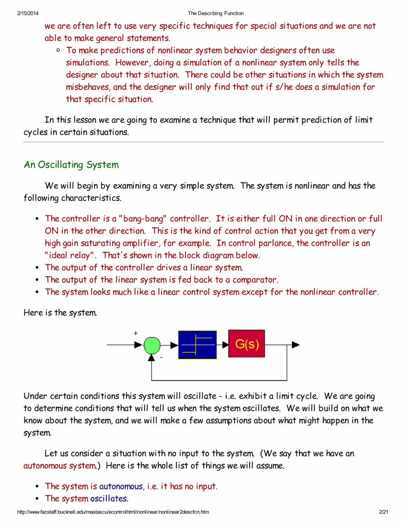
The controller is a "bang-bang" controller. It is either full ON in one direction or full

ON in the other direction. This is the kind of control action that you get from a very

high gain saturating amplifier, for example. In control parlance, the controller is an

"ideal relay". That's shown in the block diagram below.

The output of the controller drives a linear system.

The output of the linear system is fed back to a comparator.

The system looks much like a linear control system except for the nonlinear controller.

Here is the system.

Under certain conditions this system will oscillate - i.e. exhibit a limit cycle. We are going

to determine conditions that will tell us when the system oscillates. We will build on what we

know about the system, and we will make a few assumptions about what might happen in the

system.

Let us consider a situation with no input to the system. (We say that we have an

autonomous system.) Here is the whole list of things we will assume.

The system is autonomous, i.e. it has no input.

The system oscillates.



At any point in the system there will be a periodic signal.

G(s) is a system that is a low-pass filter.

In actuality it may be a motor, or some other device that consumes large chunks

of power, but the important point is the form of the transfer function. When we

say that the system is a low-pass filter we mean that it has a DC gain, and that

the frequency response drops off as you go up in frequency.

Now, it isn't obvious, but under those conditions, if the system oscillates, then the

oscillations at the output of the closed loop system will be almost sinusoidal. We need to

work through the argument that leads to that conclusion.

Let's start by asssuming that the system is oscillating. Remember, we are working on

the system shown below.

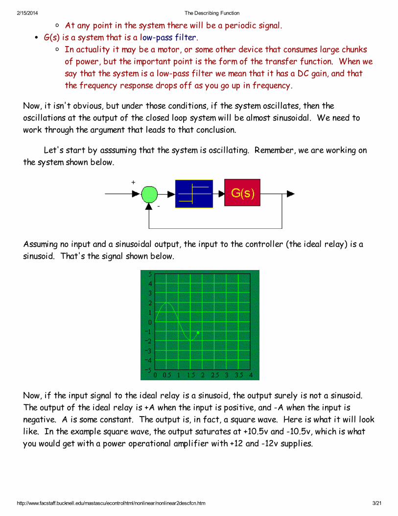
Assuming no input and a sinusoidal output, the input to the controller (the ideal relay) is a

sinusoid. That's the signal shown below.

Now, if the input signal to the ideal relay is a sinusoid, the output surely is not a sinusoid.

The output of the ideal relay is +A when the input is positive, and -A when the input is

negative. A is some constant. The output is, in fact, a square wave. Here is what it will look

like. In the example square wave, the output saturates at +10.5v and -10.5v, which is what

you would get with a power operational amplifier with +12 and -12v supplies.



Now, you have to consider what happens to the square wave as it goes through the transfer

function, G(s). Remember that we are assuming that G(s) is the transfer function of a low-

pass filter. The periodic signal out of the ideal relay can be described by a Fourier Series.

If we have a square wave that "flips" between +A and -A, the Fourier series is given by:

What is important here is that the periodic signal - the square wave above - is composed of

sinusoids at different frequencies and that G(s) is the transfer function of a low-pass

filter. Here's what we need to argue and be sure of.

When the system oscillates, the output of the ideal relay - also the input to G(s) - is

periodic.

Periodic signals can be represented by a Fourier Series representation.

G(s) is a low-pass filter.

G(s) will selectively filter out the higher frequencies in the Fourier Series, and it will

slectively pass the lower frequencies.

Now, we are going to examine a particular system. Here is the block diagram of the

system. This block diagram is taken from a Simulink block diagram that was used to

calculate the response of the system. (Note, in this system, the ideal relay had no dead zone,

and the output amplitudes were +10.5 and -10.5, which would correspond to a saturating

operational amplifier with 12v supplies.)



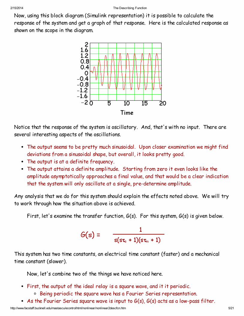
Now, using this block diagram (Simulink representation) it is possible to calculate the

response of the system and get a graph of that response. Here is the calculated response as

shown on the scope in the diagram.

Notice that the response of the system is oscillatory. And, that's with no input. There are

several interesting aspects of the oscillations.

The output seems to be pretty much sinusoidal. Upon closer examination we might find

deviations from a sinusoidal shape, but overall, it looks pretty good.

The output is at a definite frequency.

The output attains a definite amplitude. Starting from zero it even looks like the

amplitude asymptotically approaches a final value, and that would be a clear indication

that the system will only oscillate at a single, pre-determine amplitude.

Any analysis that we do for this system should explain the effects noted above. We will try

to work through how the situation above is achieved.

First, let's examine the transfer function, G(s). For this system, G(s) is given below.

This system has two time constants, an electrical time constant (faster) and a mechanical

time constant (slower).

Now, let's combine two of the things we have noticed here.

First, the output of the ideal relay is a square wave, and it it periodic.

Being periodic the square wave has a Fourier Series representation.

As the Fourier Series square wave is input to G(s), G(s) acts as a low-pass filter.



That implies that signals will be attenuated as they pass through G(s).

The higher frequency signals will be attenuated more.

If G(s) has a good drop-off, the output of G(s) may well be pretty much the

fundamental of the Fourier Series. Higher frequency terms will be attenuated,

possible pretty severely.

If G(s) filters out everything but the fundamental (and we will assume that for now)

then, we can focus on the fundamental.

Since the system oscillates with no input, the output of the system will be the

input of the system - after we account for the sign change in the comparator.

That means that the output magnitude has to equal the input magnitude.

If also means that the output phase has to be shifted by -180o.

Now, given all of the above, the first thing we are going to do is to compute the

frequency at which the phase shifts by exactly -180o. We have chosen the transfer function

to be one where we can do that analytically (i.e. do a pencil and paper calculation).

Normally, you would probably have to use a Bode' plot for G(s) to determine that frequency.

So, let's look at the transfer function again. First, we will expand the denominator.

We do that because we will be better able to compute the point where phase shifts by

exactly -180o. (Click here if you want a the details on these computations in a shorter web

page.)

Since we are interested in frequency response we let s = jw. Then the frequency

response function, G(jw), becomes:

We want to compute the frequency at which the phase shifts by exactly -180o. Notice that

we always get exactly -90o from the integrator term, so we need to compute the frequency

for which we get -90o from the quadratic term. We'll get exactly -90o from the quadratic

term when the real terms disappear. To do that we must have:

-w2tetm+ 1 = 0

or:

http://www.facstaff.bucknell.edu/mastascu/econtrolhtml/StudyGuides/NyquistExample3rdOrdSyst.htm



This should give us the frequency of oscillation of the closed loop system. Let's check that

for the example system. In the example system, we had:

te= 0.1

tm= 1.0

Computed oscillation frequency: wo= 3.16 rad/sec, or f = 0.5Hz.

Measured oscillation frequency: 5 cycles from t = 7 sec. to t = 18 sec. (estimated from

the graph above).

fmeas = 5/11 = 0.45Hz.

Given the accuracy of our estimates, this looks to be pretty close.

Now, that's the frequency, but we need to know the amplitude as well.

The amplitude of the oscillations can be computed fairly easily in this situation. We

know the Fourier Series of the relay output. That is repeated below.

The fundamental is 4A/p . Let us work on only the fundamental frequency component for a

while. That component is at a frequency of:

We can compute how the fundamental component changes as it passes through G(s).

Remember that the frequency response is given by:

And, at the oscillation frequency, wo, the magnitude of the frequency response can be

computed as:

Then, note that at the oscillation frequency, wo, we have:



And, for the time constants for the example system, this works out to be 0.091. That means

that the output of G(s) will have a fundamental component with a magnitude of:

.091(4A/p )

For the system we simulated, we chose A = 10.5, which is about what you would get from a

saturating operational amplifier with +12v and -12v supplies. That yields an amplitude of

1.215v. Comparing that to the response, the amplitude seems to be on the money.

So, it seems like we have a good method for predicting the magnitude and frequency of

oscillations in this kind of system. There are just a few unresolved questions.

We didn't account for the higher frequency components in the signal.

We may not be able to proceed as easily if we don't have an ideal relay. We need to

be able to handle other kinds of nonlinearities.

Let's get the first question out of the way. Higher frequency components must be

accounted for, and we haven't done that. Since there is no component at twice the

fundamental, let's look at the component at three times the fundamental. At that frequency,

the frequency response has a magnitude of .008. Now, if we compute the magnitude of this

component we have:

Magnitude of component at 3xfundamenal = .008(4A/3p )

= .036v

So, comparing the first few components of the output signal we have (after computing



another point):

Output Freq Magnitude

Fund 1.215v

3xFund .036v

5xFund .0057v

So, the output isn't a pure sine wave, but the harmonic content is not that large. Our

assumption that the output was sinusoidal was a fairly good assumption.

So, our conclusion has to be that this is a reasonable way to predict oscillations in a

system with an ideal relay. Here are the main points in the argument.

The controller is a "bang-bang" - i.e. an "ideal relay" - controller. It is either full

ON in one direction or full ON in the other direction.

The output of the controller drives a linear system.

The output of the linear system is fed back to a comparator.

That means that the block diagram of the system is the one below.

The process you use to analyze the system is as follows:

Assume that the relay output is a symmetrical square wave.

Determine where G(jw) has a phase shift of -180o. Call that frequency wo.

If the phase shift never reaches -180o, then the system probably does not

oscillate.

Calculate how large the fundamental signal is coming out of the transfer function G(s)

at wo.

Check that harmonics are not large because there is an assumption that the output is a

sine wave, and anything else might modify the relay input in a way that invalidates our

assumption of a symmetrical square wave out of the relay.

Other Nonlinearities



If the nonlinearity is not a ideal relay, then the analysis above must be modified.

Another common situation would be a saturating amplifier. In that case, the block diagram

would look like the one below.

Now, if we want to determine whether the system oscillates we need to account for the

saturating amplifier. However, the output of the saturating amplifier is more complex than a

square wave, and the Fourier Series for the output will now have a fundamental component

that has a magnitude dependent upon the magnitude of the input sinusoid. The problem now is

to incorporate that fact into our analysis.

Let's assume that there is a sinusoid at the input of the nonlinearity - the saturating

amplifier. Here is a plot of the output of the saturating amplifier against the input

amplitude, A. In the plot the saturation levels are -10.5v and +10.5v.

Shown below is an example of a sine wave that saturates at +10.5 and at -10.5v. You can set

the amplitude of the sine wave by typing in a value in the text box provided. Be prepared

for a little "noise" when you type. The sine wave can react instantaneously. Click the

button to start after you type in your first value, but you can change amplitude "on the fly".



We want to be able to compute the fundamental component of a general signal like the one

above, where the size of the sine part is variable, and the saturation takes place at a fixed

level, but at at different angle within the sine wave as the size/amplitude of the sine part

varies.

Let's consider what we are going to do.

We will assume that the signal resembles the one above. In particular:

We assume that they system is operating so that the saturation region is reached.

The symmetry of the signal above will ensure that it is composed of only sines,

with no cosine components.

The symmetry of the signal above also ensures that only odd harmonics are

present.

We will represent the signal by the following:

SatSine(t) = Asin(2pft) for 0 < t < ts.

SatSine(t) = Asat for ts < t < T/4.

We will compute the sine component of the fundamental.

We will assume what is a standard/typical representation of the Fourier Series

in which the typical term is ancos(2pnft) + bnsin(2pnft).

Givne that, the fundamental component is give by the expression below.

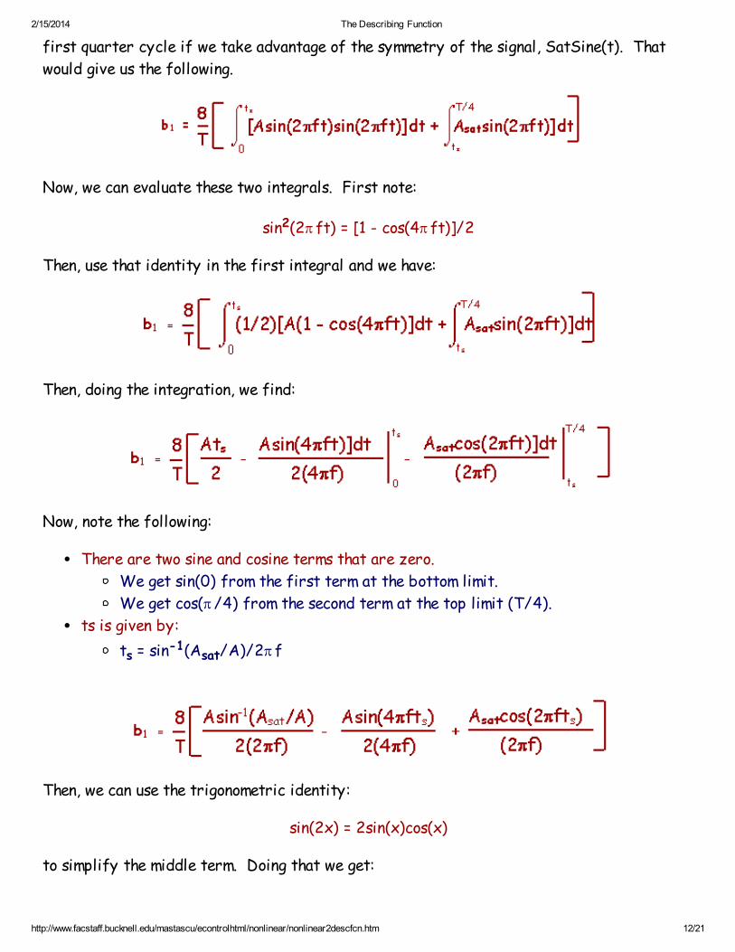
Actually, we can simplify the integral a little bit because we only need to integrate over the



first quarter cycle if we take advantage of the symmetry of the signal, SatSine(t). That

would give us the following.

Now, we can evaluate these two integrals. First note:

sin2(2pft) = [1 - cos(4pft)]/2

Then, use that identity in the first integral and we have:

Then, doing the integration, we find:

Now, note the following:

There are two sine and cosine terms that are zero.

We get sin(0) from the first term at the bottom limit.

We get cos(p/4) from the second term at the top limit (T/4).

ts is given by:

ts = sin-1(Asat/A)/2pf

Then, we can use the trigonometric identity:

sin(2x) = 2sin(x)cos(x)

to simplify the middle term. Doing that we get:



Now, we can take advantage of what we know about some of these quantities. For example,

we know:

Asin(2pfts) = Asat

So:

sin(2pfts) = Asat/A

Then, we can say:

Then, finally, we have:

or:

Now, sum up what we know.

If the input to a saturating element is a sinusoidal signal, then we have:

The output is a sine wave as long as the saturating element does not saturate. For

our calculations above, we have assumed a gain of 1.0 in this situation.

When the input is large enough to saturate the saturating element, the output has

a Fourier series and the first term has the magnitude given above as b1 above.

In doing the analysis above, we assumed that the saturating element had a gain of 1.0

until it saturated, and then saturated at a value of Asat.

The next question is how do we use the information we have above. Let's go back to the

system we began this section with. That's shown below.



Now, let's note the following.

First, we assume that the input is zero, and that we want to know whether or not the

system will oscillate.

Secondly, we note that, if the system oscillates, there will be a sort of "steady state"

in the system. In other words, the system may oscillate, but the oscillations will not

grow or decay.

If the oscillations do not grow or decay, then as we go around the loop (say we start

from the input to the saturating element) the signals may get larger or smaller, but by

the time we get around the entire loop we have to have the same signal we started with.

We are going to make the same assumptions we made for the system we examined

earlier - the ideal relay system. Those assumptions are:

The output is periodic, and thus can be represented with a Fourier Series.

G(s) is a low pass system and filters out any harmonics, so that the output of G(s)

is only the fundamental in the Fourier Series.

We can examine the implications of all this. In effect, we are saying that the loop gain has

to be exactly one, at least for the fundamental. Let's look at the result we had earlier, but

cast things in the form of a gain for the fundamental component of the output signal.

The term on the right - the "equivalent gain" is the describing function. It is a function of

the input amplitude, A, and we will represent it as DF(A). It's not really a gain because it is

not constant. It depends on the input amplitude, A. Here is a plot of the describing

function plotted against A, the input amplitude to the nonlinearity.



Note the following about this function.

For small amplitude inputs the gain is one.

A gain of 1.0 is what you expect since the system is operating linearly and the

gain is one in the linear region.

For amplitudes larger than the saturation level the "gain" decreases.

A decrease in gain should be expected because the amplitude of the output (at the

fundamental frequency) continues to increase, but reaches a limit. (In the limit,

as the input amplitude gets larger and larger, the output will look like the output

of an ideal relay. However, while the output amplitude does not increase, the

input increases and the ratio of output - at the fundamental - to the input goes

down - just like the graph shows.

However, that might be good because there might be an amplitude for which the loop gain is

one. First, rewrite the describing function as below.

Let's go back to the block diagram of the system. That's shown again below.

Now, treat the nonlinearity as a "variable gain" using the Describing Function. That means

that we will focus on the equivalent block diagram below.



Then, taking into account the gain of the describing function, the gain of G(jw) and the

change in sign in the comparator/subtractor in the loop, we have to have the following for

sustained oscillations.

DF(A)G(jw) = -1

or

G(jw) = -1/DF(A)

Example

Let's see how this can be applied. Let's look at a particular system. It is similar to

what we have been considering, but it has a gain of 50 in front of the saturation. That will

simulate an amplifier that saturates at -10.5 and +10.5v. Here is the system.

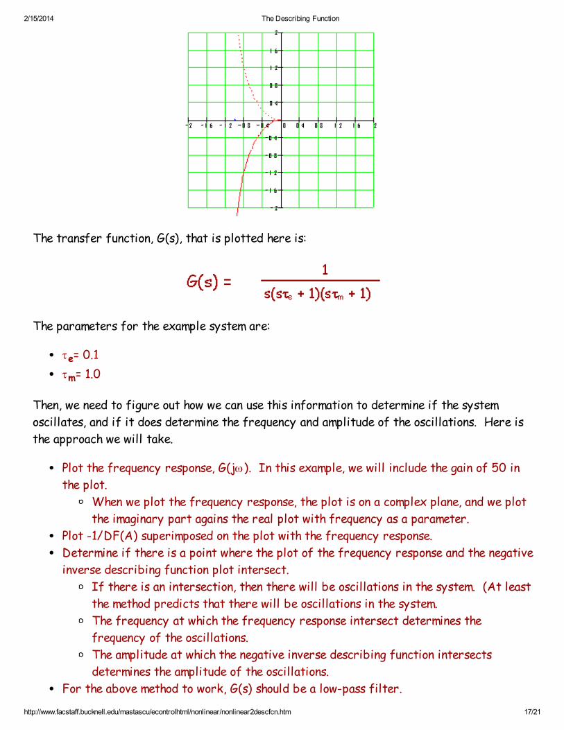
First, we need to consider how we can plot G(jw). The plot of choice is the Nyquist plot -

not a Bode' plot, not a Nichols Chart, whatever. The Nyquist plot for the transfer function

we are using as an example is shown below. This plot does not contain the gain of 50 in the

amplifier.



The transfer function, G(s), that is plotted here is:

The parameters for the example system are:

te= 0.1

tm= 1.0

Then, we need to figure out how we can use this information to determine if the system

oscillates, and if it does determine the frequency and amplitude of the oscillations. Here is

the approach we will take.

Plot the frequency response, G(jw). In this example, we will include the gain of 50 in

the plot.

When we plot the frequency response, the plot is on a complex plane, and we plot

the imaginary part agains the real plot with frequency as a parameter.

Plot -1/DF(A) superimposed on the plot with the frequency response.

Determine if there is a point where the plot of the frequency response and the negative

inverse describing function plot intersect.

If there is an intersection, then there will be oscillations in the system. (At least

the method predicts that there will be oscillations in the system.

The frequency at which the frequency response intersect determines the

frequency of the oscillations.

The amplitude at which the negative inverse describing function intersects

determines the amplitude of the oscillations.

For the above method to work, G(s) should be a low-pass filter.



Now, let's work through the steps outlined above. Here is a plot of the frequency response

and the negative inverse describing function shown together. The frequenc response is shown

in red and the negative inverse describing function is shown in blue. Adding a gain of 50 to

G(s) expands the frequency response plot, and the low frequency portion goes off scale. The

negative inverse descsribing function has a dot at -1 to show the value of the describing

function for a range of amplitudes up to the saturation value.

The frequency response intersects the negative inverse describing function at around -4.8.

At that point we can do the following computations.

The system should oscillate.

The frequency of oscillation - as determined from the frequency response - is 0.5 Hz.

Here we note that we computed the frequency at which G(jw) has a phase shift of

-180o above, and found that frequency to be 0.5 Hz.

The amplitude is found by determining when the describing function has a value of

1/4.8. That's about about .208. To determine that, we need to examine the plot of the

describing function.



Estimating the point at which DF(A) = 0.21, that looks to be around A = 60. That gives

us the input to the saturation element. That's the output of an amplifier with a gain of

50, so the input to the amplifier is 1.2, and that also has to be the magnitude of the

output. We aren't concerned about the sign here, only the magnitude of the

oscillations.

Summarizing our predictions, we have:

The system oscillates.

The frequency of oscillation is 0.5 Hz.

The amplitude of the oscillations at the system output is 1.2.

We can check these predictions by doing a simulation in Simulink. Here is the system we will

use.

Compare this simulation with the block diagram of the system just for reference.

Then, examine the computed response of the system. That is shown below.



We can compare the computed response with our predictions. Here is the comparison

The system oscillates. That's what we predicted.

The predicted frequency of oscillation is 0.5 Hz.

Measuring the frequency, we count 10 periods in 20 seconds, for a frequency of

0.5 Hz. That's what we predicted.

Notice that we examine the portion where we seem to be getting sustained

oscillations.

The predicted amplitude of the oscillations at the system output is 1.2.

The oscillations seem to have an amplitude of 1.25 or a little more compared to

the 1.2 that was predicted. That's close but not right on. We'll accept that.

Summary

We can summarize what has been presented in this lesson.

Nonlinear systems can exhibit sustained oscillations at a particular amplitude and

frequency.

A Describing Function is a kind of nonlinear gain that determines the ratio of the

fundamental of a periodic output of a nonlinearity when the nonlinearity is excited by

a sinusoidal input.

Using the describing function and the frequency response of the linear portion of the

system - which must have a low-pass transfer function it is possible to determine the

following:

Whether oscillations occur, and if they do occur to find:

Amplitude of the oscillations

Frequency of the oscillations

To determine the above, plot the frequency response of the linear portion of the

system using a Nyquist plot, and on the same plot superpose a plot of the negative

inverse of the describing function. The intersection will permit determination of

amplitude and frequency of the oscillations.

What if?

There are several points that should be noted.

The linear portion of the system is assumed to be a low-pass. That filters out any

harmonics in the periodic signal, and makes the assumption of a sinusoidal input to the

nonlinearity realistic. That's what allows you to use a describing function.

The nonlinearities we have examined here are "memoryless". In other words, the

output depends only upon the present value of the input. Nonlinearities that have



hysterisis may not depend only upon the present outut, and in those cases, the

describing function might be complex to account for phase shift in the fundamental.

These considerations may mean that you have to modify your analysis. In those cases

you may or may note have the comfort of a describing function analysis, and you may have to

rely upon doing simulations (using Simulink, for example) to compute response for various

sets of circumstances.

Problems

Problem Nonlinear1P01

Send us your comments on these lessons.

http://www.facstaff.bucknell.edu/mastascu/econtrolhtml/Problems/Nonlinear/Nonlinear1P01.htm

mailto:[email protected]

the describing function

Documents

analysis of nonlinear

behavior of nonlinear

control systems

analysis of linear systems

control system analysis

simple system

behavior ofnonlinear

linear analysis techniques