the design and analysis of d-optimal split-plot …support.sas.com/resources/papers/sixsigma2.pdfthe...

A SAS White Paper

The Design and Analysis of D-optimal Split-Plot Designs Using JMP® Version 6 Software

Table of Contents

Introduction.................................................................................................................................. 1

Basic Concepts of Experimental Design ................................................................................... 1

Split-Plot Designs........................................................................................................................ 2

Considerations for Using Split-Plot Designs .............................................................................. 3

Examples of Split-Plot Designs.................................................................................................. 4

Example 1: Completely Randomized Split-Plot Design ......................................................... 4

Example 2: Randomized Complete Block Split-Plot Design .................................................. 5

JMP 6 Design Capabilities for Creating and Analyzing Split-Plot Designs ............................ 7

Generating D-optimal Split-Plot Designs Using the Custom Design Platform in JMP 6 ....... 8

Example 1: Examining the Effect of Different Cooking Methods (CR Design) .......................... 9

Generating the D-optimal CR Split-Plot Design ..................................................................... 9

Example 2: Determining the Effect of Annealing Temperature on the Breaking Strength of

Metal Alloys (RCB Design) ...................................................................................................... 14

Generating the D-optimal RCB Split-Plot Design................................................................. 15

Example 3: Comparing Veterinary Surgery Methods for Repairing the Anterior Cruciate

Ligament (Repeated Measures Approximation) ...................................................................... 22

Generating a D-optimal Split-Plot Design as a Repeated Measures Approximation ........... 22

Example 4: Effect of Baking Temperature on Diameter of Baked Prepackaged Refrigerator

Cookies (Split-Plot Covariate).................................................................................................. 28

Generating a D-optimal Split-Plot Design with an Uncontrolled Covariate........................... 30

Example 5: Determining Factors in the Strength of a Bread Wrapper Seal (Response

Surface Design)....................................................................................................................... 37

Generating a D-optimal Response Surface Split-Plot Design.............................................. 38

Comparison of JMP 6 Split-Plot Designs with Examples from Statistical References........ 42

Example 1: Protein Extraction Experiment (Response Surface Design).................................. 43

Generating a D-optimal CCD Split-Plot Design Using JMP 6 .............................................. 44

Computing the Determinant of the D-optimal Split-Plot Design ........................................... 46

Comparisons of the Two Designs........................................................................................ 48

Example 2: Vinyl Seat Cover Experiment (Mixture Design)..................................................... 49

Generating the Mixture Split-Plot Design from Kowalski, Cornell, and Vining ..................... 49

Generating a D-optimal Mixture Split-plot Design in JMP 6 ................................................. 53

Comparison of the Two Designs.......................................................................................... 56

Conclusion ................................................................................................................................. 57

Bibliography............................................................................................................................... 57

Appendix 1: Frequently Asked Questions about the Custom Design Platform.................. 58

General.................................................................................................................................... 58

D-optimal Split-Plot Design...................................................................................................... 62

Diagnostic Tools and Options.................................................................................................. 63


1

Introduction

An experiment is a process or study that results in the collection of data. The results of experiments are not known in advance. Usually, statistical experiments are conducted when researchers can manipulate the conditions of the experiment and control the factors that are relevant to the research objectives. For example, a rental car company might compare the tread wear of four brands of tires, while controlling the type of car, speed, road surface, weather, and driver. However, there are situations in which a condition is difficult to manipulate. For example, it might be difficult to change the temperature of a furnace from 400º C to 350º C and then back to 400º C. In such an experiment, results will have to be collected on the low setting first and then the high setting, without alternating the temperature between runs. There are many types of experimental designs, and each design is analyzed using specific statistical methods. For an experiment in which a factor has levels that are hard to change, using a split-plot design is best. The focus of this paper is to discuss the concepts of D-optimal split-plot design and respective analyses using JMP 6. If you have a strong statistical background and are familiar with JMP, you might want to skip the next three sections and go directly to the section “Generating D-optimal Split-Plot Designs Using the Custom Design Platform in JMP 6”. Note: Frequently asked questions about the Custom Design platform are presented in Appendix 1.

Basic Concepts of Experimental Design

At each stage of the planning process for an experiment, many decisions must be made about the design. Here are the four main steps for designing an experiment.

1. Define the problem and the questions to be addressed. 2. Define the population of interest. 3. Determine the need for sampling. 4. Define the experimental design.

These steps are not independent, and it might be necessary to revise earlier decisions that were made during the planning process for the designed experiment. A clear definition of the details of the experimental design makes the desired statistical analyses possible and generally improves the usefulness of the results. Planning an experiment properly is very important in order to ensure that the right type of data and sufficient sample size and power are available to answer the research questions as clearly and efficiently as possible. However, every experiment can be separated into the treatment structure and the design structure. How the treatment structure and design structure components are combined determines the appropriate design, model, and statistical analysis and is described as follows:

1. Identify the experimental unit. An experimental unit is the entity to which a level of a factor or levels of combinations of factors are applied and observed.

2. Identify the types of factors. Factors are variables.


2

3. Define the treatment structure. The treatment structure refers to the factors or factor combinations being studied.

4. Define the design structure. The design structure consists of those factors that are constructed by grouping the experimental units into blocks of homogeneous experimental units (for example, completely randomized design, randomized complete block design, split-plot design, and so on).

5. Replicate. Replication is the independent application of a factor level or combination of levels to an experimental unit.

6. Determine error variance. Error variance is the variation between experimental units that are treated alike.

7. Define the model that will be used as the basis for the statistical analysis. In order to define the appropriate model, you must be able to identify the experimental unit as well as the treatment and design structures for each experimental unit.

Split-Plot Designs

The split-plot design has existed for many years and recently has drawn attention in the industry due to the practical implications of using these designs instead of randomized block designs or completely randomized designs. Complexities can occur during the execution of an experiment as a result of restricted randomization. Typical situations that occur in experimental designs include those in which

• one or more of the factors in an experiment are considered hard-to-change. As a result, the run order of the treatments is determined by these factors

• experimental units are processed together as a group or batch for one or more of the factors and are processed individually for other factors

• the settings of the factor levels are not re-set in design runs that follow sequentially where some factors have the same setting in each run.

These situations generally result in some type of split-plot design structure. Split-plot designs have a different number of experimental units than other traditionally designed experiments. In the split-plot design, the levels of the hard-to-change factor or factors are assigned at random to the large experimental unit (also known as the whole plot). The large experimental units are then divided into smaller experimental units (the subplot), and the levels of the second factor are assigned at random to the smaller experimental unit within the larger experimental unit. JMP 6 randomizes the split-plot design, which you can see as you examine each row of a design data table. Split-plot design names are prefixed with the name that’s associated with the whole plot design, for example, randomized complete block (RCB) split-plot design. The design for the subplot is never given, but it is, by definition, a randomized block design.


3

Considerations for Using Split-Plot Designs

Split-plot designs provide the following advantages:

• They permit the efficient use of factors that require large experimental units in combination with other factors that require small experimental units.

• They provide increased precision in the comparison of some factors. • They permit the introduction of new treatments into an experiment that is already in

progress.

However, split-plot designs also have some disadvantages:

• The statistical analysis is complicated because different comparisons have different error variances. (JMP 6 provides the statistical analysis easily, thereby eliminating this disadvantage.)

• Low precision on the estimate for the variance component on the whole plot can result in large differences being non-significant, while small differences on the subplots might be statistically significant even though they are of no practical significance.

Split-plot designs are most effective in two specific situations:

• for experiments in which one factor is defined as the larger (hard-to-change) experimental unit as compared to other factors in the design

• when introducing a new factor into an experiment that is already in progress. In the split-plot design, the levels of hard-to-change (whole plot) factors are estimated from the large experimental units. The subplot effects consist of the subplot factors and the interaction of the whole plot and subplot factors and are estimated from the small experimental units. Because there are two sizes of experimental units, there are two experimental errors (one for each experimental unit). The JMP Fit Model platform generates the split-plot analysis under the Restricted Maximum Likelihood (REML) Variance Components Estimates and Fixed Effect Tests (Display 1). The REML Variance Component Estimates Table reports estimates for the whole-plot error and the residual error. The Fixed Effect Test Table reports the F ratio and p-value associated with the whole plot, the subplot, and the interaction of whole plot and subplot effects.


4

Display 1. Split-Plot Analysis Using the Fit Model Platform in JMP 6 Generally, the error that is associated with the Residual (subplot) is smaller than the whole plot error because

• smaller experimental units within the large experimental units tend to be positively correlated. This has the effect of reducing experimental error.

• error degrees of freedom for the whole plots are usually less than those for the subplots. This has the effect of increasing the whole-plot error relative to that of the subplots.

The net effect is that the whole-plot factor is less precisely estimated than the subplot factor and its interaction with the whole-plot factor. This difference in precision should be taken into consideration when deciding to use a split-plot design.

Examples of Split-Plot Designs

Two designs that are commonly used are the completely randomized (CR) split-plot and the randomized complete block (RCB) split-plot design. The completely randomized split-plot design is the simplest experimental design. This section provides examples for both the CR and the RCB split-plot designs.

Example 1: Completely Randomized Split-Plot Design

This completely randomized split-plot example evaluates the strength of fabric. Factor F represents the two types of fabric rolls that were assigned at random to the whole plots, and factor P represents three types of polymers that were assigned at random to the subplot within the


5

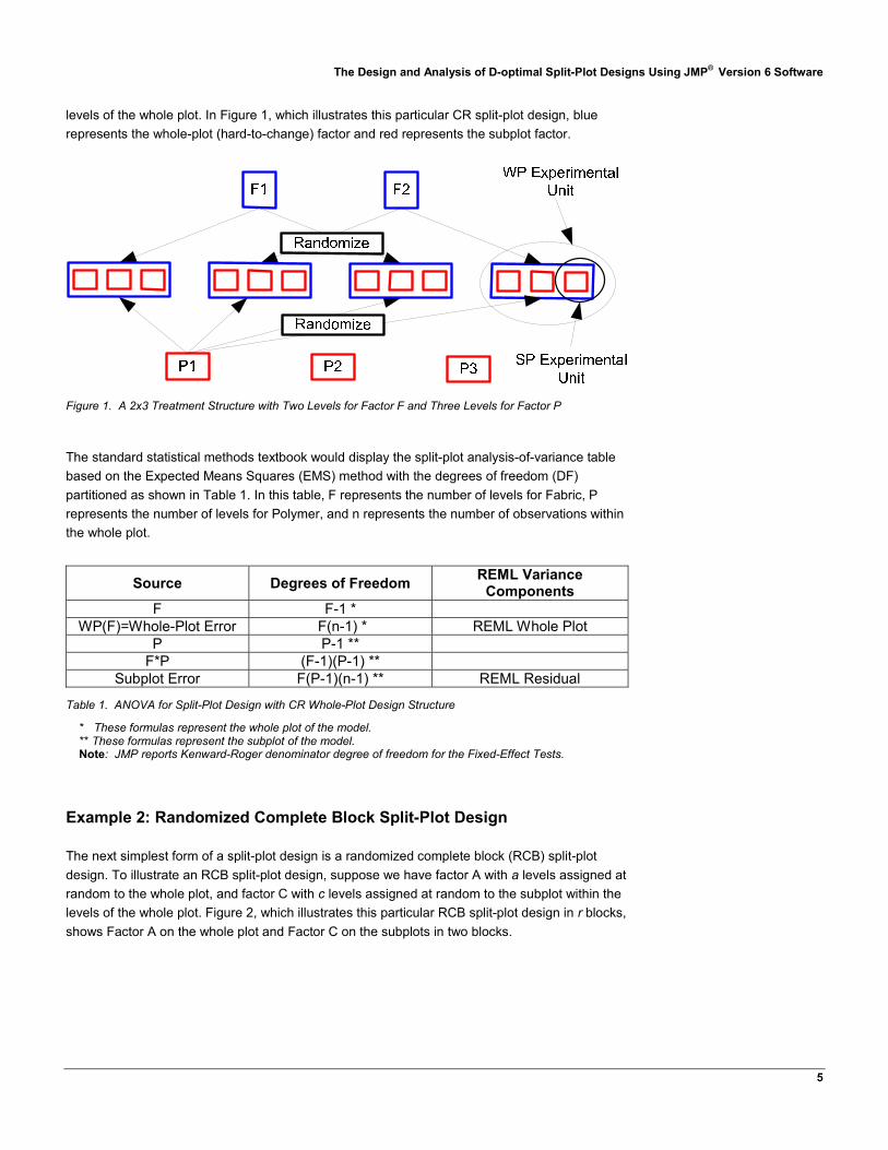
levels of the whole plot. In Figure 1, which illustrates this particular CR split-plot design, blue represents the whole-plot (hard-to-change) factor and red represents the subplot factor.

Figure 1. A 2x3 Treatment Structure with Two Levels for Factor F and Three Levels for Factor P The standard statistical methods textbook would display the split-plot analysis-of-variance table based on the Expected Means Squares (EMS) method with the degrees of freedom (DF) partitioned as shown in Table 1. In this table, F represents the number of levels for Fabric, P represents the number of levels for Polymer, and n represents the number of observations within the whole plot.

Source Degrees of Freedom REML Variance Components

F F-1 * WP(F)=Whole-Plot Error F(n-1) * REML Whole Plot

P P-1 ** F*P (F-1)(P-1) **

Subplot Error F(P-1)(n-1) ** REML Residual

Table 1. ANOVA for Split-Plot Design with CR Whole-Plot Design Structure

* These formulas represent the whole plot of the model. ** These formulas represent the subplot of the model. Note: JMP reports Kenward-Roger denominator degree of freedom for the Fixed-Effect Tests.

Example 2: Randomized Complete Block Split-Plot Design

The next simplest form of a split-plot design is a randomized complete block (RCB) split-plot design. To illustrate an RCB split-plot design, suppose we have factor A with a levels assigned at random to the whole plot, and factor C with c levels assigned at random to the subplot within the levels of the whole plot. Figure 2, which illustrates this particular RCB split-plot design in r blocks, shows Factor A on the whole plot and Factor C on the subplots in two blocks.


6

Figure 2. Randomized Complete Block Split-Plot Design with Factor A on the Whole Plot and Factor C on the Subplot in Two Blocks Standard statistical methods textbooks display the randomized complete block split-plot analysis-of-variance table based on EMS method with the degrees of freedom (DF) partitioned as shown in Table 2. In this table, R represents the number of levels of blocks, A represents the number of levels of Factor A, and C represents the number of levels of Factor C.

Source Degrees of Freedom REML Variance Components

Blocks R-1 * A A-1 *

Whole-Plot Error (A-1)(R-1) ** REML Whole Plot C C-1 **

A*C (A-1)(C-1) ** Subplot Error A(R-1)(C-1) ** REML Residual

Table 2. ANOVA for Split-Plot Design with RCB Whole-Plot Design Structure

* These formulas represent the whole plot of the model.

** These formulas represent the subplot of the model.

Note: JMP reports Kenward-Roger denominator degree of freedom for the Fixed-Effect Tests.

A1 A3A2 A2A1A3

Block 1 Block 2

C1 C2 C3 C4 C1 C2 C3 C4

Randomize Randomize

Randomize Randomize

WP Experimental

Unit

SP Experimental

Unit


7

JMP 6 Design Capabilities for Creating and Analyzing Split-Plot Designs

JMP 6 is the first software with the capability to generate D-optimal split-plot designs. The JMP 6 Custom Design algorithm for generating these designs is based on Goos (2002). The main advantage of the D-optimal designs (including D-optimal split-plot designs) that are included with JMP 6 is that they can be created for

• any number of observations • any number of explanatory variables • any statistical model • any combination of qualitative and quantitative variables • any experimental region.

The Custom Design platform allows you to define different types of factors in an experimental design using the Add Factor button, as shown in Display 2.

Display 2. Add Factor Drop-Down Menu You can choose from seven factors on the drop-down menu:

• Continuous refers to quantitative factors with two levels (low and high). • Categorical refers to nominal factors. JMP allows an arbitrary number of levels. • Blocking refers to factors that involve controlling a known source of variation by

grouping the units under study based on a common characteristic of the blocking factor, and there is no restriction on the number of runs per block. JMP allows an arbitrary number of runs per block. JMP 6 defines the design role for blocking factors as a FIXED effect.

• Covariate refers to factors that already have unchangeable values and JMP designs around these values.

• Mixture refers to factors composed of ingredients. A minimum of three ingredients are required in JMP.

• Constant refers to factors that are fixed during an experiment. • Uncontrolled refers to factors that you know have an effect on the response but which

you cannot measure in advance. They are measured during the process and are used in the modeling process. In order to set the minimum sample size appropriately, the uncontrolled factors need to be defined because the researcher does not have any control over them.


8

The whole plot and subplot factors can be defined as either categorical or continuous. The whole plot factor(s) are defined by setting the changes specification as HARD in the Custom Designer. You may have multiple factors on the whole plot and subplot. The Custom Design platform generates a script that provides the correct statistical analysis for split-plot designs that estimate two variance components: the whole-plot error component, and the residual error component. At the current time, the JMP 6 Custom Design platform does not generate designs for more complex split-plot designs such as split-split-plot or split-split-split-plot designs because these designs involve estimating more than two variance components. However, the JMP Fit Model platform can perform the statistical analysis for complex split-plot designs provided the effects in the model are correctly specified. Also, the JMP 6 Custom Design platform does not generate Bayesian split-plot designs, I-optimal split-plot designs, or nonlinear split-plot designs. The Fit Model platform in JMP provides two methods to estimate variance components: Expected Mean Squares (EMS) and Restricted Maximum Likelihood (REML). The EMS method can be used when the data is balanced. REML is an iterative method and can be used when the data is balanced or unbalanced. The estimates for the variance components for EMS and REML are equivalent only in balanced data. Researchers and statisticians commonly use REML to estimate variance components rather than EMS. REML is the default method in JMP 6 and is the recommended method. If you are generating a design using the Custom Design platform, the data table will include a model script that will use the REML method to estimate the variance components. JMP 6 also provides the Kenward-Roger computation for the denominator degrees of freedom (DF) in Fixed-Effect tests.

Generating D-optimal Split-Plot Designs Using the Custom Design Platform in JMP 6

This section illustrates various experiments that use split-plot designs created with the Custom Design platform in JMP. Each example

• describes the experiment • details the steps used to create the split-plot designs with the Custom Design platform • provides the statistical analysis for each experiment.

The following aspects of the Custom Design platform are helpful to know when you create split-plot designs and generate the analysis.

• A random seed can be set to ensure that the same design is generated for repeated designs. The examples in the following section use the random seed 1207513. In general, you do not need to define a random seed when generating designs.

• If you use any option other than Default to set the number of runs in a split-plot design, the number of whole plots will change when you click the Back button. The generated designs are all valid designs. However, if you do not use Default to set the number of runs and then use the Back button, it is important that you enter the number of whole plots and number of runs that were used on the initial split-plot design to maintain the number of whole plots and number of runs.

• You should also use the default REML method rather than the EMS method. The Custom Design platform's algorithm for estimating the variance components is designed to use the REML method.


9

Example 1: Examining the Effect of Different Cooking Methods (CR Design)

This first example examines the effect of different cooking methods (steam, stir fry, microwave) on the retention of folic acid in four vegetables: spinach, bean sprouts, cabbage, and green beans. The experiment is conducted as follows. A sample of vegetable (for example, spinach) is chopped up. The sample is divided into three portions. One portion is randomly assigned to each of the three cooking methods. After cooking, the amount of folic acid that was retained is measured for each portion. There were a total of 16 samples (four samples of each vegetable). There were a total of 48 portions (three portions of each of the 16 samples). This experiment can be described by the following linear model:

ijkikkijiijk ey +++++= )(αββωαµ

In this model,

• ijky = Folic Acid mcg

• µ = intercept (overall mean response of all observations)

• iα = Vegetables effect of the ith level of α

• ijω = whole-plot error, assumed iid N(0, 2

ωσ )

• kβ = Cooking Method effect of the kth level of β

• ik)(αβ = interaction effect of Vegetables by Cooking Method of the ith level of α

with the kth level of β

• ijke = subplot error, assumed iid N(0, 2σ )

ijω and ijke are assumed to be independent of one another.

Generating the D-optimal CR Split-Plot Design

You can generate the D-optimal CR split-plot design using the JMP 6 Custom Design platform, as follows:

1. Select DOE Custom Design. 2. Click the red triangle next to Custom Design and select Set Random Seed. Then type

1207513 if you want to exactly replicate our results. 3. Click OK. 4. In the DOE Custom Design window under Responses, double-click Y to change the

name of the response and type Folic Acid Amount (Display 3).


10

Display 3. The Custom Design Window with Settings for Responses and Factors Categories

5. In the DOE Custom Design window under Factors, select Add Factor Categorical 4 Level.

6. To change the name of the factor, double-click X1 and type Vegetables. 7. Under Changes, click Easy and select Hard. 8. Click L1 and type Spinach. 9. Press the Tab key and type Sprouts. 10. Press the Tab key and type Cabbage. 11. Press the Tab key and type Green Beans. 12. Under Factors, select Add Factor Categorical 3 Level. 13. To change the name of the factor, double-click X2 and type Cooking Method. 14. Click L1 and type Steam. 15. Press the Tab key and type Stir Fry. 16. Press the Tab key and type Microwave. 17. Select Continue. 18. In the DOE Custom Design window under Model, select Interactions 2nd. The

Vegetable*Cooking Method interaction effect should appear in the model. If it does not appear, make sure the names of the factors are not highlighted.

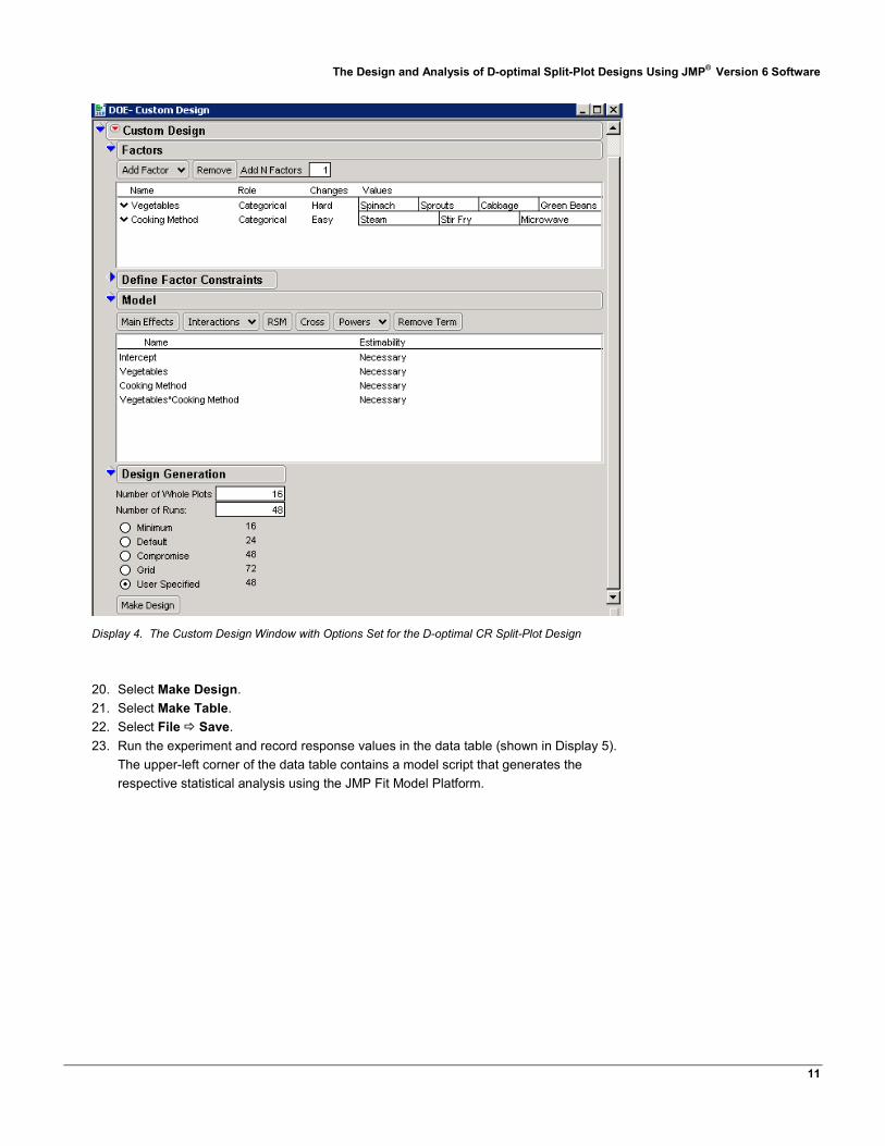
19. Under Design Generation (shown in Display 4), change Number of Whole Plots from 12 to 16 and Number of Runs from 24 to 48.


11

Display 4. The Custom Design Window with Options Set for the D-optimal CR Split-Plot Design

20. Select Make Design. 21. Select Make Table. 22. Select File Save. 23. Run the experiment and record response values in the data table (shown in Display 5).

The upper-left corner of the data table contains a model script that generates the respective statistical analysis using the JMP Fit Model Platform.


12

Display 5. Data Table for the D-optimal CR Split-Plot Design

24. Select File Save. 25. To run the model, click the red triangle next to Model and select Run Script to display

the Fit Model window (shown in Display 6).


13

Display 6. Running the Model from the Fit Model Window

26. Select Run Model in the Fit Model window to see the analysis shown in Display 7.


14

Display 7. Significance of the Effects in This Model In this analysis, the Cooking Method interaction (under the Fixed-Effect Tests category) is significant at the 1% level. Notice that both main effects, Vegetables and Cooking Method, are significant at the 1% level.

Example 2: Determining the Effect of Annealing Temperature on the Breaking Strength of Metal Alloys (RCB Design)

The second split-plot design example illustrates the effect of annealing temperature on the breaking strength of three experimental metal alloys. In a research laboratory, a metallurgist has four laboratory ovens that are each capable of annealing three metal samples. The metallurgist decides to use a split-plot design with temperatures assigned to ovens as the hard-to-change factor (whole plot) and metal samples within ovens as subplots. The temperature levels assigned to whole plots were 675, 700, 725, and 750. The alloys assigned to subplots were designated as A1, A2, and A3. The metallurgist can make only one run per day in the experimental ovens. He decides to use a randomized block design for the ovens (whole plots) with three blocks, using days as a categorical factor for the blocks. Furthermore, there is a restriction of 12 runs per day.


15

This experiment can be described by the following linear model:

ijkijjikikijk ery ++++++= )(αββωαµ

In this model,

• ijky = Breaking Strength


• kr = Day effect of the kth block

• iα = Temperature effect of the ith level of α

• ikω = whole-plot error assumed iid N(0, 2

ωσ )

• jβ = Alloy effect of the jth level of β

• ij)(αβ = interaction effect of Temperature by Alloy of the ith level of α with the jth

level of β


ikω and ijke are assumed to be independent of one another.

Generating the D-optimal RCB Split-Plot Design

You can generate the D-optimal RCB split-plot design using the JMP 6 Custom Design platform, as follows:

1. Select DOE Custom Design. 2. Click the red triangle next to Custom Design and select Set Random Seed. Then type

1207513 in order to replicate our results. 3. Click OK. 4. In the DOE Custom Design window under Responses, double-click Y to change the

name of the response and type Breaking Strength. 5. In the DOE Custom Design window under Factors, select Add Factor Categorical

4 Level. 6. To change the name of the factor, double-click X1 and type Temperature. 7. Under Changes, click Easy and select Hard. 8. Click L1 and type 675. 9. Press the Tab key and type 700. 10. Press the Tab key and type 725. 11. Press the Tab key and type 750. 12. Under Factors, select Add Factor Categorical 3 Level. 13. To change the name of the factor, double-click X2 and type Day. 14. Click L1 and type 1. 15. Press the Tab key and type 2. 16. Press the Tab key and type 3. 17. Under Changes, click Easy and select Hard.


16

18. Under Factors, select Add Factor Categorical 3 Level. 19. Double-click X3 and type Alloy. 20. Click L1 and type A1. 21. Press the Tab key and type A2. 22. Press the Tab key and type A3. 23. Select Continue (Display 8).

Display 8. The Custom Design Window with Settings for Responses and Factors Categories

24. Under Factors, select Temperature. 25. Under Model, select Alloy. 26. Select Cross (Display 9).

Note: The Temperature*Alloy interaction should be listed in the model window.


17

Display 9. The Custom Design Window with All Settings for the Experiment

27. Under Design Generation, specify the Number of Whole Plots as 12 and the Number of Runs as 36, as shown in Display 9.

28. Select Make Design. 29. Select Make Table. 30. Select File Save. 31. Run the experiment and record response values in the data table. Notice that the upper-

left corner of the data table (shown in Display 10) contains a model script that will generate the respective statistical analysis using the JMP Fit Model Platform.


18

Display 10. Data Table for the D-optimal RCB Split-Plot Design

32. Select File Save. 33. To run the model, click the red triangle next to Model. Then select Run Script to display

the Fit Model window (Display 11).


19

Display 11. The Fit Model Window for the RCB Design

34. Select Run Model in the Fit Model window to see the analysis shown in Display 12.


20

Display 12. Significance of the Effects in This Model In this analysis, the Temperature*Alloy interaction is barely significant at the 5% level, while both main effects (Temperature and Alloy) are significant at the 1% level. The Day effect is not significant. Under the Effect Details button, you will see that each effect has a pop-up menu. These pop-up menus enable you to request tables, plots, and tests for that effect. The commands listed for an effect append results to the effect report. Optionally, you can close results or dismiss the results by deselecting the item in the menu. For example, suppose you want to see the LSMeans plot for the Temperature*Alloy interaction. To generate this plot,

1. Click the blue diamond next to Effect Details. 2. Scroll to Temperature*Alloy Interaction. 3. Click the red triangle next to Temperature*Alloy. 4. Select LSMeans Plot.

The resulting LSMeans plot for the Temperature*Alloy interaction is shown in Display 13.


21

Display 13. LSMeans Plot for the Temperature*Alloy Interaction You can see from the plot that there is a slight indication that the difference between alloys depends on temperature. Alloy and temperature differences are highly significant. Breaking strength was highest at all temperatures for alloy A3 and lowest at all temperatures for alloy A1. To see the LSMeans plot for the main effect Temperature,

1. Click the blue diamond next to Effect Details. 2. Scroll to Temperature. 3. Click the red triangle next to Temperature. 4. Select LSMeans Plot.

The resulting LSMeans plot for the main effect of Temperature is shown in Display 14.

Display 14. The LSMeans Plot for the Main Effect, Temperature For all alloys, the breaking strength increases as the temperature is increased until it reaches a maximum of 725. Above 725, there is a decrease in breaking strength.


22

Example 3: Comparing Veterinary Surgery Methods for Repairing the Anterior Cruciate Ligament (Repeated Measures Approximation)

In this example, a veterinarian wants to determine which of two surgical methods is best for repairing the Anterior Cruciate Ligament (ACL) in various dogs. The ACL, a ligament that connects the tibia (leg) to the femur (thigh), serves to prevent the tibia from moving forward relative to the femur. The experiment consists of using the two surgical methods (no wrapping and TPLO) on dogs with an ACL problem and then measuring the strength of the dog’s joint at 1, 2, 3, and 4 months later. Based on other studies the veterinarian believed the ratio of the whole-plot variance to the residual was 3. In this experiment, each dog is measured more than once and can be analyzed using repeated measures analysis of variance. Because randomization of the time levels is not possible, this type of experiment is more properly analyzed as a repeated-measure design. However, the split-plot analysis will be a good first-order approximation to the proper analysis under the assumption of compound symmetry (equal variances and equal correlations) and is certainly far better than treating the data as if it came from a completely randomized design! The problem associated with split-plot-in-time is that it does not account for the correlation structure associated with the repeated measures over time. This experiment can be described by the following linear model:

ijkikkijiijk ey +++++= )(αββωαµ

In this model,

• ijky = Strength of Joint


• iα = Method effect of the ith level of α

• ijω = whole-plot error, assumed iid N(0, 2

ωσ )

• kβ = Time effect of the kth level of β

• ik)(αβ = interaction effect of Method by Time of the ith level of α with the kth

level of β


ijω and ijke are assumed to be independent of one another.

Generating a D-optimal Split-Plot Design as a Repeated Measures Approximation

You can generate the D-optimal split-plot design with repeated measures approximation as follows:

1. Select DOE Custom Design. 2. Click the red triangle next to Custom Design and select Set Random Seed. Type

1207513 in order to replicate our results.


23

3. Click OK. 4. In the DOE window under Responses, double-click Y to change the name of the

response and type Strength of Joint (Display 15).

Display 15. The Custom Design Window with Settings for the Custom Design, Responses, and Factors Categories

5. In the DOE window under Factors, select Add Factor Categorical 2 Level. 6. To change the name of the factor, double-click X1 and type Method. 7. Under Changes, click Easy and select Hard. 8. Click L1 and type No Wrapping. 9. Press the Tab key and type TPLO. 10. Under Factors, select Add Factor Categorical 4 Level. 11. To change the name of the factor, double-click X2 and type Time. 12. Click L1 and type 1. 13. Press the Tab key and type 2. 14. Press the Tab key and type 3. 15. Press the Tab key and type 4. 16. Click the red triangle next to Custom Design and select Advanced Options Split-plot

Variance Ratio. 17. In the dialog window that opens, type 3. 18. Click OK. 19. Select Continue to display the Model and Design Generation categories in the window

(Display 16).


24

Display 16. Settings for Model and Design Generation

20. Under Model, select Interactions 2nd. Note: The Method*Time interaction should be listed in the Model window.

21. Under Design Generation, specify the Number of Whole Plots as 6 and the Number of Runs as 24.

22. Select Make Design. 23. Select Make Table. 24. Sort the data table by Whole plots and time. The data table is shown in Display 17. 25. Select File Save.


25

Display 17. Data Table for the Repeated Measures as a D-optimal Split-Plot Design

26. Run the experiment and record response values in the data table. Notice that the upper-left corner of the data table (shown in Display 18) contains a model script that will generate the respective analysis using the JMP Fit Model Platform.

27. Select File Save. 28. Click the red triangle next to Model and select Run Script to display the Fit Model

window (Display 18).


26

Display 18. The Fit Model Window for the Repeated Measures Approximation

29. Select Run Model to see the analysis shown in Display 19.


27

Display 19. Significance of the Effects for the Repeated Measures Approximation This analysis indicates that there is not a significant Method*Time interaction. However, both main effects, Method and Time, are significant at the 1% level. If you examine the LSMeans tables in Display 20, you can see that there appears to be an increase in strength over time. The strength of the joint is stronger under the TPLO method.

Display 20. LSMeans Table Showing Joint Is Stronger under the TPLO Method


28

Example 4: Effect of Baking Temperature on Diameter of Baked Prepackaged Refrigerator Cookies (Split-Plot Covariate)

The next design is a split-plot design with an uncontrolled covariate that is measured on the small experimental unit (subplot). In this experiment, a baker wants to study the effect of baking temperature on the diameter (mm) of baked cookies from prepackaged refrigerator cookies. The baker selects three cookie types (sugar, peanut butter, chocolate chip) for the experiment. The recommended baking temperature is 350º, so the baker selects the temperatures 300º,350º, and 400º for the experiment. The plan for the experiment is to obtain four replications of each treatment combination. The process is to cut a slice of the cookie dough from a package of each of the cookie types, place all three cookies on a baking tray, and place the tray in the oven where the oven was set to one of the three temperatures. The diameter of the cookie after baking depends on the thickness of the slice of cookie dough. The directions on the wrappers are to make 1/4 inch or 6.25 mm slices, but it is not easy to cut slices to exactly 6.25 mm. Thus, the thickness of the cookie dough slices is measured as a possible uncontrolled covariate. The oven to which the temperature was assigned is the experimental unit for the levels of the temperature of the whole plot. The slice of cookie dough is the experiment unit for the levels of the cookie type or subplot. In this example, it is assumed that position on the baking tray is not important because there were just three cookies being baked at the same time (position on the tray could be an important source of variability and should be investigated). The process for conducting the experiment was to randomly select one of the temperatures, set the oven to that temperature, and randomly assign one cookie of each cookie type to the three positions on the baking tray when the tray is placed into the oven. The thickness of each slice of cookie dough is considered an uncontrolled covariate that is measured on the subplot experimental unit. The statistical analysis will be conducted based on analysis of covariance (ANCOVA) methods described in Milliken and Johnson (2002). Figure 3 represents the split-plot ANCOVA design for this baking cookie experiment.


29

Figure 3. Split-Plot ANCOVA Design for Cookie Experiment This experiment can be described by the following linear model:

ijkmijmjmimijmjijkiijkm ey +++++++++= )()()()( αβτβταταβτβωαµ In this model,

• ijkmy = diameter


• iα = Temperature effect of the ith level of α

• ijkω = whole-plot error assumed iid N(0, 2

ωσ )

• jβ = Cookie Type effect of the jth level of β

• mτ = Thickness effect of the mth level of τ

• ij)(αβ = interaction effect of Temperature and Cookie type of the ith level of α with

the jth level of β

• im)(ατ = interaction effect of Temperature and Thickness effect of ith level of α with the mth level of τ

• jm)(βτ = interaction effect of Cookie Type and Thickness effect of the jth level of β with the mth level of τ

Peanut Butter

Chocolate Chip

Cookie Type

Sugar

350 400 300

Temperature

Cookie is experimental unit for cookie type and slice thickness is covariate.

Oven is experimental unit for temperature

RANDOMIZE

RANDOMIZE


30

• ijm)(αβτ = interaction effect of Temperature, Cookie Type, and Thickness effect of

the ith level of α , the jth level of β with the mth level of τ

• ijkme = subplot error assumed iid N(0, 2σ )

ijkω and ijkme are assumed to be independent of one another.

Generating a D-optimal Split-Plot Design with an Uncontrolled Covariate

You can generate the D-optimal split-plot design using an uncontrolled covariate in the JMP 6 Custom Design Platform, as follows:

1. Select DOE Custom Design. 2. Click the red triangle next to Custom Design, select Number of Starts, type 10, and

click OK. 3. Click the red triangle next to Custom Design, select Set Random Seed and type

1207513 in order to replicate the results. Click OK. 4. In the DOE Custom Design window under Responses, double-click Y to change the

name of the response and type Diameter (Display 21).

Display 21. Custom Design Window with Settings for the Custom Design and Factors Categories

5. In the DOE Custom Design window under Factors, select Add Factor Categorical 3 Level.

6. To change the name of the factor, double-click X1 and type Temperature. 7. Under Changes, click Easy and select Hard. 8. Click L1 and type 300. 9. Press the Tab key and type 350. 10. Press the Tab key and type 400. 11. Under Factors, select Add Factor Categorical 3 Level.


31

12. To change the name of the factor, double-click X2 and type Cookie. 13. Click L1 and type Peanut Butter. 14. Press the Tab key and type Chocolate Chip. 15. Press the Tab key and type Sugar. 16. Under Factors, select Add Factor Uncontrolled and leave the values as missing. 17. Double-click X3 and type Thickness. 18. Select Continue to display the Model and the Design Generation categories in the

window (Display 22).

Display 22. Settings for Model and Design Generation

19. Under Model, select Interactions 3rd. The model should include these effects: Intercept, Temperature, Cookie, Thickness, Temperature*Cookie, Temperature*Thickness, Cookie*Thickness, and Temperature*Cookie*Thickness.

20. Under Design Generation, specify the Number of Whole Plots as 12 and the Number of Runs as 36.

21. Select Make Design. 22. Select Make Table. 23. Measure the thickness of the cookies prior to baking them and record those values in the

Thickness column. Display 23 shows the values used in this experiment.


32

Display 23. Analysis Data Table Showing Values for Cookie Thickness

24. Bake the cookies. Then measure the diameters and record them in the data table (Display 24).


33

Display 24. Analysis Data Table Showing Cookie Diameter for This Experiment

25. Click the Thickness column in the data table. 26. Under Column Properties, remove Coding and then click OK. You need to remove

Coding so that the actual values for the uncontrolled covariate are used. 27. Select File Save. 28. To run the model, click the red triangle next to Model and select Run Script to display

the Fit Model window (Display 25).


34

Display 25. The Fit Model Window for the Design with an Uncontrolled Covariate

29. Click the red triangle next to Model Specification; then remove the check mark next to Center Polynomials. Because you are following the methods described in Milliken and Johnson (2002), you do not need to center polynomials for this particular analysis.

30. Select Run Model. When you run the model, you get the analysis shown in Display 26.


35

Display 26. Model Analysis in the Custom Design – Fit Least Squares Window The first step includes

• simplifying the covariate part of the model • deleting the highest-order interaction term involving the covariate that is not significant • refitting the model.

For this particular experiment, Temperature*Cookie*Thickness effect was deleted first (Display 27).


36

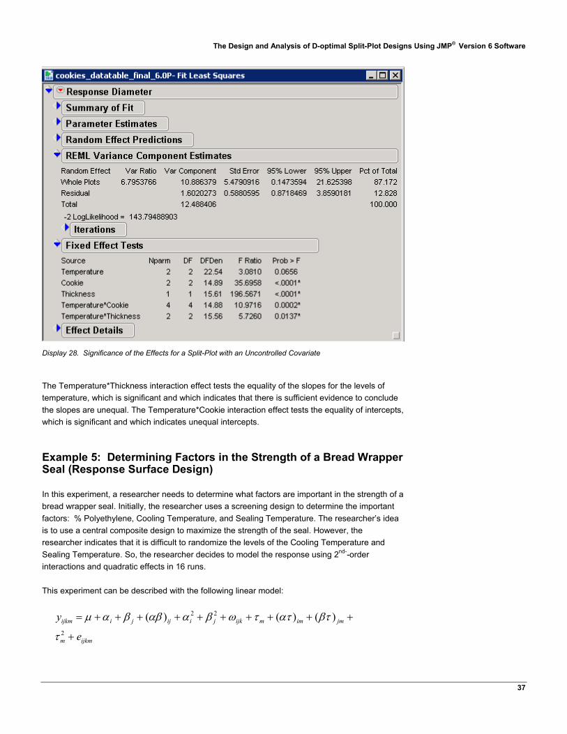
Display 27. Significance of the Effects of a Split-Plot with an Uncontrolled Covariate The Cookie*Thickness effect was deleted second. Those deletions leave the model with the following effects (Display 28):

• Temperature • Cookie • Thickness • Temperature*Cookie • Temperature*Thickness


37

Display 28. Significance of the Effects for a Split-Plot with an Uncontrolled Covariate The Temperature*Thickness interaction effect tests the equality of the slopes for the levels of temperature, which is significant and which indicates that there is sufficient evidence to conclude the slopes are unequal. The Temperature*Cookie interaction effect tests the equality of intercepts, which is significant and which indicates unequal intercepts.

Example 5: Determining Factors in the Strength of a Bread Wrapper Seal (Response Surface Design)

In this experiment, a researcher needs to determine what factors are important in the strength of a bread wrapper seal. Initially, the researcher uses a screening design to determine the important factors: % Polyethylene, Cooling Temperature, and Sealing Temperature. The researcher’s idea is to use a central composite design to maximize the strength of the seal. However, the researcher indicates that it is difficult to randomize the levels of the Cooling Temperature and Sealing Temperature. So, the researcher decides to model the response using 2nd--order interactions and quadratic effects in 16 runs. This experiment can be described with the following linear model:

ijkmm

jmimmijkjiijjiijkm

e

y

+

++++++++++=2

22 )()()(

τ

βταττωβααββαµ


38

In this model,

• ijkmy = Strength of Seal


• iα = Cooling Temperature effect of the ith level of α

• jβ = Sealing Temperature effect of the jth level of β

• ij)(αβ = interaction effect of Cooling Temperature and Sealing Temperature of the ith

level of α with the jth level of β

• 2

iα = quadratic effect of Cooling Temperature, α

• 2jβ = quadratic effect of Sealing Temperature, β

• ijkω = whole-plot error assumed iid N(0, 2

ωσ )

• mτ = % Polyethylene effect of the mth level of τ

• im)(ατ = interaction effect of Cooling Temperature and % Polyethylene effect of ith level of α with the mth level of τ

• jm)(βτ = interaction effect of Sealing Temperature and % Polyethylene effect of the jth

level of β with the mth level of τ

• 2mτ = quadratic effect of % Polyethylene, τ

• ijkme = subplot error, subplot error, assumed iid N(0, 2σ )

ijkω and ijkme are assumed to be independent of one another.

Generating a D-optimal Response Surface Split-Plot Design

You can generate the D-optimal response surface split-plot design using the Custom Design platform, as follows:

1. Select DOE Custom Design. 2. Click the red triangle next to Custom Design and select Set Random Seed. Type

1207513 in order to replicate our results. 3. Click OK. 4. In the DOE Custom Design window under Responses, double-click Y to change the

name of the response and type Strength of Seal (Display 29).


39

Display29. Settings for the Responses and Factors Categories in the Custom Design Window

5. In the DOE Custom Design window under Factors, click in the box next to Add N factors and type 3.

6. Select Add Factor Continuous. 7. For the first factor, under Changes, click Easy and select Hard. 8. To change the name of the factor, double-click X1 and type Cooling Temperature. 9. Press the Tab key and type 120. 10. Press the Tab key and type 140. 11. Press the Tab key and type Sealing Temperature. 12. Under Changes, click Easy and select Hard. 13. Click -1 and type 220. 14. Press the Tab key and type 240. 15. Press the Tab key and type % Polyethylene. 16. Press the Tab key and type 85. 17. Press the Tab key and type 90. 18. Select Continue. 19. Under Model, select Interactions 2nd (Display 30).


40

Display 30. Settings for the Model and Design Generation Categories Added

20. Under Model, select Power 2nd. 21. Under Design Generation, specify Number of Whole Plots as 12 and Number of

Runs as 16. 22. Select Make Design. 23. Select Make Table. 24. Select File Save. 25. Run the experiment and record response values in the data table, shown in Display 31.

Notice that the upper-left corner of the data table contains a model script that will generate the respective statistical analysis using JMP’s Fit Model platform.

26. Select File Save.


41

Display 31. Analysis Data for the D-optimal Response Surface Split-Plot Design

27. Click the red triangle next to Model and select Run Script to display the Fit Model window (shown in Display 32).

Display 32. The Fit Model Window for the Response Surface Design


42

28. Select Run Model to see the analysis shown in Display 33.

Display 33. Significance of the Effects in This Model

In this experiment, the tests of Fixed Effects indicate that for this particular design, the main effects (Cooling Temperature, Sealing Temperature, and %Polyethylene) are significant at the 5% level. There is also significant interaction of Cooling Temperature and %Polyethylene and with Sealing Temperature and %Polyethylene at the 5% level. In addition, there appears to be a significant quadratic effect for the %Polyethylene at the 5% level.

Comparison of JMP 6 Split-Plot Designs with Examples from Statistical References

This section is a brief discussion of the advantages of JMP methods for D-optimal split-plot designs over traditional methods. A commonly cited example in statistical literature for a response surface split-plot design is the Trinca & Gilmour (2001) protein extraction experiment, and a common example in literature for the mixture split-plot design is the Kowalski, Cornell, and Vining (2002) experiment for the production of vinyl for automobile seat covers. Goos (2002) demonstrates how the intention with these designs was good, but the methods used in these designs were limited. However, JMP 6 can generate D-optimal split-plot designs that are better than those cited in references. It is also important to recognize that, even with the latest software,


43

it is of the utmost importance to generate the design correctly to obtain good statistical analysis for models. The following examples discuss designs generated via traditional methods and how those same designs compare when generated in JMP 6.

Example 1: Protein Extraction Experiment (Response Surface Design)

Trinca and Gilmour (2001) considered a response surface design with a split-plot unit structure. Their protein extraction example involves five three-level factors, with one factor (feed position) held constant each day and four factors varied within a day. Their proposed 42-run split-plot design is a face-centered central composite design (CCD) with 16 factorial runs, 20 axial points, and six center point replicates, partitioned into 21 whole units of size two. Display 34 shows a JMP data table with the same design considered in the Trinca and Gilmour experiment. The following sections illustrate the steps used to create the design with JMP and then compare the two designs that are created using these two methods.

Display 34. JMP Data Table for Response Surface Design with a Split-Plot Unit Structure


44

Generating a D-optimal CCD Split-Plot Design Using JMP 6

You can generate the D-optimal CCD Split-Plot design in JMP, as follows:

1. Select DOE Custom Design. 2. Click the red triangle next to Custom Design and select Set Random Seed. 3. In the dialog window that opens, type 1207513. 4. Click OK. 5. Click the red triangle next to Custom Design and select Save X Matrix

(Display 35).

Display 35. Settings for Factors in the Custom Design

6. Click the red triangle next to Custom Design. Then select Number of Starts and type 10.

7. In the DOE Custom Design window under Factors, click the box next to Add N factors and type 5.

8. Select Add Factor Continuous. 9. To change the name of the factor, double-click X1 and type W. 10. Under Changes, click Easy and select Hard. 11. Leave the levels at -1 and 1 for all the continuous factors. 12. To change the name of the factor, double-click X2 and type S1. 13. Double-click X3 and type S2. 14. Double-click X4 and type S3. 15. Double-click X5 and type S4. 16. Select Continue. 17. Under Model, select Interactions 2nd (Display 36).


45

Display 36. The Custom Design Window with Settings Ready to Make the Design

18. Under Model, select Power 2nd. 19. Under Design Generation, specify Number of Whole Plots as 21 and Number of

Runs as 42. 20. Select Make Design. 21. Select Make Table. 22. Select File Save.

When you click Make Design, the application produces the data table that is shown in Display 37.


46

Display 37. Resulting Data Table

Computing the Determinant of the D-optimal Split-Plot Design

The determinant is not reported under the Custom Design platform. To obtain the determinant, click the red triangle next to Custom Design and select Save X Matrix. Then you can use the following steps to obtain the value of the determinant for a design using the Custom or Augment platform.

1. In the upper-left corner of the data table, click the red triangle next to the data table name.

2. Select New Property/Script to display a dialog box (Display 38) that has the two fields Name and Value.


47

Display 38. Dialog Box with the Name and Value Fields

3. In the Name field, type Compute Determinant. 4. In the Value field, type

(d = Det(X` * V Inverse * X); Show(d))

5. Click OK. 6. Click the red triangle next to Design Matrix, and select Run Script. 7. Click the red triangle next to V Inverse and select Run Script. 8. Click the red triangle next to Compute Determinant and select Run Script. 9. From the menu bar, select View, then select Log. The value of D (shown in Display 39)

represents the determinant.


48

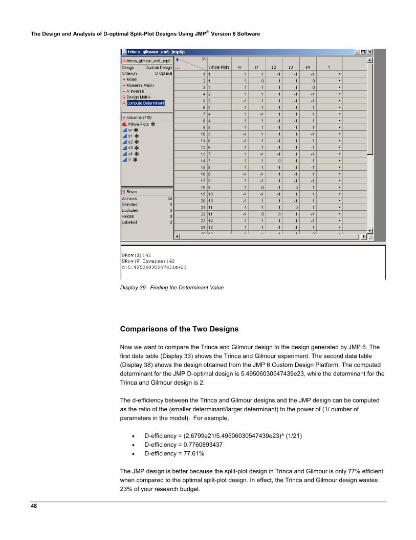
Display 39. Finding the Determinant Value

Comparisons of the Two Designs

Now we want to compare the Trinca and Gilmour design to the design generated by JMP 6. The first data table (Display 33) shows the Trinca and Gilmour experiment. The second data table (Display 38) shows the design obtained from the JMP 6 Custom Design Platform. The computed determinant for the JMP D-optimal design is 5.49506030547439e23, while the determinant for the Trinca and Gilmour design is 2.

The d-efficiency between the Trinca and Gilmour designs and the JMP design can be computed as the ratio of the (smaller determinant/larger determinant) to the power of (1/ number of parameters in the model). For example,

• D-efficiency = (2.6799e21/5.49506030547439e23)^ (1/21) • D-efficiency = 0.7760893437 • D-efficiency = 77.61%

The JMP design is better because the split-plot design in Trinca and Gilmour is only 77% efficient when compared to the optimal split-plot design. In effect, the Trinca and Gilmour design wastes 23% of your research budget.


49

Example 2: Vinyl Seat Cover Experiment (Mixture Design)

Kowalski, Cornell, and Vining (2002) describe an experiment for making vinyl for automobile seat covers. The experiment has two process variables and a mixture. The mixture contains three plasticizers with proportions designated as X1, X2, and X3. The two process variables are Rate of Extrusion and Temperature of Drying. Both process variables are continuous with two levels. The response is vinyl thickness. The researchers used a split-plot design with 28 observations and 12 center points. The data table in Display 40 shows the mixture split-plot design cited in Kowalski, Cornell, and Vining (2002). In their experiment, the reported determinant was 0.0793073251028802.

Display 40. Data from Kowalski, Cornell, and Vining Experiment Generating the Mixture Split-Plot Design from Kowalski, Cornell, and Vining

In JMP 6, you can generate the mixture split-plot design cited in Kowalski, Cornell, and Vining (2002), as follows:

1. Select DOE Custom Design. 2. Click the red triangle next to Custom Design, select Number of Starts, and

type 50. 3. Click OK. 4. Click the red triangle next to Custom Design, select Set Random Seed, and type

1207513.


50

5. Click OK. 6. In the DOE Custom Design window under Factors, click the box next to Add N

factors and type 3 (Display 41).

Display 41. The Custom Design Window for the Vinyl Seat Cover Experiment

7. Select Add Factor Mixture. 8. Leave all three mixture factors at their default labels and settings. 9. In the DOE Custom Design window under Factors, click the box next to Add N

factors and type 2. 10. Select Add Factor Continuous. 11. Double-click X4 and type Z1. 12. Double-click X5 and type Z2. 13. For both Z1 and Z2, under Changes, click Easy and select Hard. 14. Click Continue. 15. Under Factors, select X1, X2, and X3. 16. Under Model, select Interactions 2nd. This enters the interaction mixture terms. 17. Under Factors, select z1 and z2. 18. Under Model, select Interactions 2nd. This enters the only interaction effect. 19. Under Factors, select X1, X2, and X3. 20. Under Model, select z1 and z2. 21. Select Cross to enters the cross terms. 22. Under Model, select z1 and z2. 23. Select Remove Term.

As shown in Display 42, the effects in the model should be

x1 x2 x3 x1*x2 x1*x3 x2*x3 z1*z2 x1*z1


51

x2*z1 x3*z1 x1*z2 x2*z2 x3*z2

Display 42. List of Effects for the Vinyl Seat Cover Experiment

24. Under Design Generation, specify 4 for Number of Whole Plots and 16 for Number of Runs. (Note: It is not possible with the interface to design three more blocks with center points.)

25. Select Make Design. 26. Select Make Table to create the data table shown in Display 43.


52

Display 43. Data Table Created for the Vinyl Seat Cover Experiment

27. Add 12 rows to the data table by clicking Rows Menu and selecting Add Rows… 28. In the dialog window that opens, type 12. 29. Click OK. 30. In row 17, enter the following values, respectively, for X1, X2, X3, z1,and z2: .33,

.33, .33, 0, 0. 31. Copy the values from row 17 into the remaining 11 new rows. 32. Enter 5, 6, and 7 as the values for Whole Plots. 33. Select File Save.

The final data table is shown in Display 44. Note: The center points were added to obtain a better estimate of pure error.


53

Display 44. The Data Table with Final Values Added Generating a D-optimal Mixture Split-plot Design in JMP 6

The following steps are similar to those described previously by Kowalski, Cornell, and Vining; however, the design is different. You can generate a D-optimal mixture split-plot design in JMP 6, as follows:

1. Select DOE Custom Design. 2. Click the red triangle next to Custom Design. Then select Number of Starts and

type 50. 3. Click OK. 4. Click the red triangle next to Custom Design. Then select Set Random Seed and type

1207513. 5. Click OK. 6. Click the red triangle next to Custom Design and select Save X Matrix. 7. In the DOE Custom Design window under Factors, click the box next to Add N factors

and type 3 (Display 45).


54

Display 45. Factors Categories in the Custom Design Window

8. Select Add Factor Mixture. 9. Leave all three mixture factors at their default labels and settings. 10. In the DOE Custom Design window under Factors, click the box next to Add N factors

and type 2. 11. Select Add Factor Continuous. 12. Double-click X4 and type z1. 13. Double-click X5 and type z2. 14. For both z1 and z2, under Changes, click Easy and select Hard. 15. Select Continue. 16. Under Factors, select X1, X2, and X3. 17. Under Model, select Interactions 2nd to enter the interaction mixture terms. 18. Under Factors, select z1 and z2. 19. Under Model, select Interactions 2nd to enter the only interaction effect. 20. Under Factors, select X1, X2, and X3. 21. Under Model, select z1 and z2. 22. Select Cross to enter the cross terms. 23. Under Model, select z1 and z2. 24. Select Remove Term.

As shown in Display 46, the effects in the model should be

x1 x2 x3 x1*x2 x1*x3 x2*x3 z1*z2 x1*z1 x2*z1 x3*z1 x1*z2 x2*z2 x3*z2


55

Display 46. List of Effects for the JMP D-optimal Mixture Split-Plot Design

25. Under Design Generation, specify 7 for Number of Whole Plots and 28 for Number of Runs.

26. Select Make Design to create the data table shown in Display 47.


56

Display 47. Data Table Created for the D-optimal Mixture Split-Plot Design

Comparison of the Two Designs

The difference between this generated design in JMP and that described in Kowalski, Cornell, and Vining is that the JMP design does not include center points, yet, the JMP D-optimal design includes more runs. For this particular design using JMP, the determinant was 5971.37551300236.

The D-efficiency between the Kowalski, Cornell, and Vining’s design versus the JMP design is computed as follows:

• D-efficiency = (0.0793073251028802 / 5971.37551300236) ^ (1 / 13) • D-efficiency = 0.4215649858 • D-efficiency = 42.15%

Once again, this comparison shows that the D-optimal split-plot design generated by using Custom Design in JMP 6 is better because the split-plot design in Kowalski, Cornell, and Vining is only 42% efficient when compared to the optimal split-plot design. In effect, the Kowalski, Cornell, and Vining design wastes 58% of your research budget.


57

Conclusion

This paper demonstrates the capability of JMP 6 to generate D-optimal split-plot designs as well as the analysis for those designs. Some statisticians say that 95% of all experiments have randomization restrictions, or blocking. Such experiments should be modeled as split-plot designs to avoid the negative consequences that result from inappropriate designs and models, and JMP 6 now gives you the means to do that more easily. Because split-plot designs are applicable for experiments in many fields (including industry, medicine, education, agriculture, economics, psychology, and social sciences), JMP 6 is an ideal tool for researchers in any of those fields.

Bibliography

Anderson, Virgil L. and McLean, Robert A. (1974). Design of Experiments: A Realistic Approach. New York: Marcel Dekker, Inc. Goos, Peter (2002). The Optimal Design of Blocked and Split-plot Experiments. New York: Springer-Verlang. Huang, P., Chen, D., and Voelkel, J. O. (1998). "Minimum-Aberration Two-Level Split-Plot Designs," Technometrics, 40, 314--326. Kowalski, Scott M., Cornell, John A., and Vining Geoffrey G. (2002). “Split-plot Designs and Estimation Methods for Mixture Experiments with Process Variables”. Technometrics, 44(1), 72-79. Milliken, George A. and Johnson, Dallas E. (2002). Analysis of Messy Data. Volume III: Analysis of Covariance. Boca Raton: Chapman & Hall/CRC. Milliken, George A. and Johnson, Dallas E. (1992). Analysis of Messy Data. Volume I: Designed Experiments. Boca Raton: Chapman & Hall/CRC. Milliken, George A., Moore, Terri, and Stephen, Alan (2000). “Special Problems of DOE Applications within the Semiconductor”, ASA August 2000. Montgomery, Douglas C. (1997) Design and Analysis of Experiments (4th Edition). New York: John Wiley & Sons. Peterson, Roger G. (1985). Design and Analysis of Experiments. New York: Marcel Dekker, Inc. Trinca, Luzia A. and Gilmour, Steven G. (2001). “Multi-Stratum Response Surface Designs”. Technometrics, 43(1), 25-33.


58

Appendix 1: Frequently Asked Questions about the Custom Design Platform

General

When should I use a 2-level continuous factor versus a 2-level categorical factor?

Factors are the variables whose values (levels) you set to study their relationship to a response. Those factor levels that are defined as continuous represent quantitative numeric variables with a specific order setting (low, high). Categorical variables are qualitative variables with distinct (discrete) settings that have no specific order.

How can I obtain a continuous factor with more than two levels?

The only design in JMP that enables you to define a continuous factor with more than two levels is the full factorial design. For example, you can select continuous factor and define a factor with more than two levels. However, be aware that the full factorial design will generate a design with all possible runs. For example, if you have two continuous factors with four levels, two other factors with three levels, and one factor with two levels, the design will have 288 runs (4*4*3*3*2). Alternatively, there are two approaches more widely used than the full factorial design. The first approach is to design continuous factors with two levels by:

1. using the low and high values for the levels of the factors, respectively, under

Custom Design. 2. selecting powers 2, 3, and 4, if necessary, to form effects in the model. 3. entering the number of runs under Design Generation. 4. clicking the Make Design button. 5. examining the prediction variance profile to determine the relative variance.

Now, you can make any changes you want to the design points in the data table. You can use the Augment Design platform to examine the new prediction variance profile to see the impact of changing those particular design points. To use the Augment Design platform, you need to:

1. select Augment Design from the DOE Custom Design menu. 2. identify the factors and response; then click Augment. 3. enter the number of runs. 4. select Make Design.

Now, you can examine the prediction variance profile and compare it to the profile from the original custom design. The second approach is to use Custom Design but define the continuous factor as a categorical factor with the desired number of levels. This approach enables you to test the continuous factor at the exact levels you want to test. To use this approach,


59

1. Change the values of L1-LN to the value you want for the continuous variable. 2. Click Make Design. 3. Click Make Table. 4. Change the data type from character to numeric in the data table. 5. Change the modeling type from nominal to continuous. 6. Remove the design role property.

Now you can use the Augment Design platform to build powers into the model and to examine the prediction variance profile.

What is the difference between a covariate and an uncontrolled factor?

There are two types of covariates. Fixed covariates are defined prior to the experiment. Covariates that cannot be measured in advance of the experiment are uncontrolled factors. Covariate and uncontrolled factors are commonly known as nuisance factors, but they are important factors to include in generating designs as they can help to explain the variability in the response. In JMP, the covariate factor must exist in a data table or factors table. If only covariate factors are in the data table, then the row-exchange is used to find the optimal subset. If there are other factors in addition to covariate factors, then row exchange is used to find the optimal subset of covariate factors with respect to all the model terms involving only the covariate factors. After the row exchange the covariate runs are fixed and the coordinate exchange is done to optimize the settings of the other factors with respect to the covariates. The covariate factor is randomized under the Custom DOE if any factor is set to hard. The covariate factor will remain in the order of the candidate set if all factors are set to easy.

What do the values Easy and Hard mean for a factor’s Changes specification?

The specification of Easy or Hard as a value for Changes is associated with the levels of each factor type. The specification for the Changes indicates the difficulty of changing the level of a factor value from run-to-run. Changing any one factor from Easy to Hard results in JMP generating a split-plot design.

What is the difference between a blocking factor and a factor with a change specification set to Hard?

Blocking involves controlling a known source of variation by grouping the experimental units so that the conditions under which the treatments are observed are as homogeneous as possible. A blocking factor is an experimental factor that might contribute to the response variability but which is otherwise not of interest. A blocking scheme is used in a factorial design to account for variability in the response that may otherwise be attributed incorrectly to other factors or to experimental error. In designs with factors whose Changes specifications include Hard and Easy, there are two different sizes of experimental units. With a block design, there is only one set of experimental units. Blocks can be considered as fixed or random effect. Blocks are typically random effects while factors whose Changes specification is set to Hard are typically fixed effects. JMP 6 defines the design role for the blocking factors as a fixed effect.


60

When should you use a blocking factor versus a categorical factor to define a block variable?

When there is no restriction on the number of runs per block, the blocking factor can be used. If there is a restriction on the number of runs per block, then a categorical factor should be used to define the block variable.

What is the difference between a fixed effect and a random effect?

Factors that are defined as fixed are limited to those factors that are specified in the experimental design and inferences from the design are confined to the type and range of independent variables in the model. An effect is random if you have observed a sample of levels of an effect and want to generalize from those levels to a larger population of possible levels.

How can you reproduce the same design?

1. Click the red triangle next to Custom Design. 2. Select Set Random Seed. 3. Type a positive number to ensure the same design is generated for repeated

designs. How can you reproduce the same run order for a design?

The Set Random Seed option ensures that you create the same design every time. It does not ensure that you get the same run order every time. If you want the same run order, then you would use the Run Order "Keep the Same" if it is available. This will enable you to get the same run order every time. For some designs such as randomized block designs, you cannot reproduce the same run order. Some designs such as split-plot designs do not have the capability for Run Order “Keep the Same”. For those designs if you want the same randomization of run order, then after you have created a data table with the run order you can add a new column by using the following formula:

If(Row() == 1, Random Seed(123456); Random SeededUniform(), Random SeededUniform())

Then you can sort the data table on this newly created column, and you will have the same randomized run order.

How do you decide which design and analysis to use for an experiment?

It is important to generate the experimental design and respective statistical analysis based on criteria determined in the planning stages of the experiment. You should not try to generate the experimental design based on the analysis. It is the experimental design that determines the analysis. Consult with a statistician at your site for help with generating designs or statistical analyses.


61

It is understandable that you would try to reproduce designs from textbooks or references when you are learning to use the software or teaching courses. Experiments conducted with restricted randomization need to implement the restricted randomization in the design and the analyses. Also, keep in mind that two or more researchers can generate an experimental design and can a have different order for randomization of the runs; both designs are valid.

What services can I expect from JMP Statistical Technical Support?

JMP Statistical Technical Support is responsible for • directing customers to the appropriate JMP platform for the particular type of analysis

that they request. It is the customer's responsibility to determine which type of design or analysis is appropriate for their needs.

• answering questions concerning specific details of the statistical platforms, such as discussing available options and limitations.

• providing references for formulas and statistical techniques used by our algorithms where possible.

• providing the customer with limited guidance and references for interpreting the output produced by JMP.

• investigating reported problems in JMP and passing those that we verify to the software development team for response.

• providing limited and general statistical advice as we deem necessary on a case-by-case basis.

Due to our limited knowledge of any particular customer's data analysis situation, we cannot provide general statistical consulting services such as selection of statistical methodology or design of experiments. Nor can we provide customized JSL code for a customer's specific needs. For statistical assistance beyond the services we provide above, consider consulting a local statistician or posting your question to a newsgroup (support.sas.com/faq/003/FAQ00351.html).

Can a response surface design have both qualitative (nominal) and quantitative (continuous) factors?

Yes, a response surface can have both qualitative and quantitative factors. You can generate such a response surface design with the Custom Design platform.

Are all of the DOE platforms scriptable in JMP 6?

Currently, only the Custom Design platform can be scripted. Can you use the Custom Design platform to reproduce screening or response surface designs that are identical to those designs generated using the Screen Design platform or the Response Surface Design platform?

You can generate screening designs with the Custom Design platform that are identical to those in the Screening platform provided that you follow the appropriate steps in the Custom Design platform. Response surface designs (such as Box-Behnken and Central Composite

http://support.sas.com/faq/003/FAQ00351.html


62

designs) are not generally optimal, so the Custom Design platform does not reproduce them. By default, the Custom Design platform generates I-optimal response surface designs.

D-optimal Split-Plot Design

Does SAS software or JMP have the capability to generate split-plot designs?

Both SAS software and JMP provide the capability to generate split-plot designs and the respective analysis. In the SAS/STAT module, the PLAN procedure can generate full factorial split-plot designs, while the ADX interface in the SAS/QC module generates both full factorial and fractional factorial split-plot designs. The type of fractional factorial split-plot designs generated in the ADX interface is a class of minimum aberration designs based on Huang, Chen, and Voelkel (1998). The respective analysis is done using the MIXED procedure. In addition, JMP, which was also developed at SAS, can generate D-optimal split-plot designs and the respective statistical analysis.

Does JMP provide prospective sample size and power computations for split-plot designs?

JMP 6 does not provide prospective sample size and power computations for split-plot designs.

How does JMP determine the number of whole plots and runs in a split-plot design?

The Design Generation Panel for a split-plot design is slightly different than other D-optimal designs in Custom Design. The dialog allows one to define the number of whole plots and runs for a split-plot design. The default number of whole plots is generally set to half the default number of runs. The exception is when this number is insufficient to fit all the whole plot fixed effects and also provide a degree of freedom for estimating the whole plot variance. In that case, JMP increases the number of whole plots to this minimum value. The default number of runs is chosen to try to create a balanced design if that is possible. For example, if there are some factors at two levels and some categorical factors at three levels, then the default sample size will be a multiple of six that is large enough to fit the a priori model. There is a dynamic tension in the choice of the number of whole plots. Convenience and economics dictate that the number of whole plots be as small as possible. However, estimating the whole plot variance accurately suggests increasing the number of whole plots.

Are there any guidelines for determining the number of whole plots and runs in a design?

One guideline that might help when deciding on the number of whole plots would be to consider a number that represents the number of times you are willing to change the hard-to-change factor(s).

What happens if you specify a missing value for the number of whole plots and the number of runs?

If you specify a missing value for the number of whole plots, JMP will determine the optimum number of whole plots for you. This approach will provide enough whole plots to estimate the variance among whole plots.


63

Does JMP generate split-plot designs with more than two variance components?

The JMP 6 Custom Design platform does not generate designs for more complex split-plot designs such as split-split-plot or split-split-split-plot designs because these designs involve estimating more than two variance components. Generating designs with more than two variance components for more complex split-plot designs is under consideration for future enhancements to the Custom Design platform. However, the JMP Fit Model platform can perform the statistical analysis for complex split-plot designs provided the effects in the model are correctly specified.

Does JMP generate I-optimal split-plot designs, Bayesian split-plot designs, or nonlinear split-plot designs?

The JMP 6 Custom Design platform does not generate Bayesian split-plot designs, I-optimal split-plot designs, or nonlinear split-plot designs. Bayesian and I-optimal split-plot designs are under consideration for future enhancements to the Custom Design platform.

Should I select Show Diagnostics to compare split-plot designs?

No, you should NOT select Show Diagnostics to compare split-plot designs nor should you use any of the efficiencies or the average variance of prediction from Show Diagnostics. The D-efficiency for a split-plot design can be computed as the ratio of the (smaller determinant/larger determinant) to the power of (1/ number of parameters in the model). You can use a script to compute the determinant and the D-efficiency for split-plot design.

How can I add center points to a split-plot design?

There is no explicit support for center points in split-plot designs. The recommendation for adding center points is to arbitrarily add a center point to any desired whole plot or construct a whole plot entirely of center points.

Diagnostic Tools and Options

How do I use the prediction variance profile and the prediction variance surface?

You can use the prediction variance profile plot to determine the prediction variance relative to the error variance, which is useful in comparing designs at a point of prediction. The prediction variance surface is a 3-D representation of variance surface. In the prediction variance profile, the numbers at the bottom in black represent the levels associated with your factors in the design. For example, suppose you have a factor called TEMP with two levels, 70 and 90. The variance prediction profile will display in black 70 and 90. A categorical factor with two levels, No and Yes. The prediction profile will display No and Yes. The red value for Variance on the left side is the relative variance. It is relative to the actual experimental error variance. This value is multiplied by the actual variance in the experiment (MSE). For demonstration purposes, assume that the prediction variance value is 0.298522, the prediction variance will be about 30% of the error variance due to the implicit replication in a sample size based on the number of runs in the design.


64

Initially, all continuous factors are set to the center value and categorical factors are set to the first level. The prediction points can be changed by moving the red vertical lines. If you do this, the prediction variance is updated for each new point moved to. You can also use the Prediction Variance Profiler to obtain the maximum prediction variance. The goal is to minimize the prediction variance for the experimental design.

What information is provided under the alias matrix, and how should it be used?

The alias matrix only appears for custom designs with two factor interactions if all factors are at two-levels. The table shows the aliasing (if any) between the model terms and all the two-factor interactions. The alias matrix enables you to see the confounding pattern in D-optimal or I-Optimal designs.

What does the Relative Variance of Coefficients table represent, and how is it used?

For designs with factors scaled to the range, [-1 1], the minimum value of the relative variance of a coefficient is 1/sample size. Two-level full and fractional designs meet this lower bound. In general, if the values of the relative variance of the coefficient are all the same, that is an indication of a high degree of symmetry (or balance) in the design. The decision about whether a given variance is acceptably small depends on two things. First, it depends on what you believe the process variability is because the standard error of the coefficient is the square root of the relative variance times the mean square error (MSE) of the model. Second, it depends on how big an effect needs to be to have practical significance. If the standard error of the coefficient is less than 2 or 3 times this size, then you will be able to detect effects that are large enough for you to care about. If the standard error of the coefficient is roughly the same size as an effect that would matter to you, then you need a lot more data (4 times as much roughly). Rather than using efficiencies for the comparison of designs you can use the relative variance of coefficients. You want to minimize the variance on the parameter estimates. The closer the values are to 0, the smaller the confidence limits about the parameter estimates the better. The larger the variance, the larger the confidence limits about the parameter estimates.

How can I obtain the efficiency associated with a design, and what is the correct way to use the efficiency of a design?

In the Custom Design dialog window, click the red triangle next to Custom Design and select Show Diagnostics (you can make this selection after you generate the design). There are no guidelines for acceptance or rejection of efficiency measures for a designed experiment. Efficiencies are measured on a scale from 0-100%. The efficiency for any real design might be less than 100%. It is important to remember that because these efficiencies measure the goodness of the design relative to theoretical designs that may not be possible in many cases. They are typically not useful as absolute measures of design goodness. Instead, efficiency measures should be used relatively to compare designs for the same situation. Thus, in order to use


65

efficiencies to compare designs requires the same model, same design region, and same number of runs. D-efficiency and A-efficiency are two measures of precision of the parameter estimates. G-efficiency measures the precision of the predicted values.

What is the difference between D-optimal and I-optimal designs, and which should I use for the various types of designs?

D-optimality maximizes the value of the determinant; I-optimality minimizes the value of the expected error in prediction. JMP 6 currently generates only D-optimal split-plot designs. I-optimality is the default in JMP when an RSM model is specified in Custom Design. I-optimality minimizes a measure of the expected error in prediction and should be used when the predictive capability of your fit is the primary concern, as is very often the case in industrial designs.

When should I increase the number of starts for a design?

One difficulty with the creation of optimal designs is that the methods used to generate them do not always find the optimal design in cases where the optimal design is known from theory. For example, all orthogonal designs are D-optimal with respect to a linear additive model. As the number of factors and sample size increase, the optimization problem becomes harder. It is easy for an optimizer to converge to a local optimum instead of a global optimum. It is useful to know that if random starts are used for the optimization, the design produced at the end is not always the same. Increasing the number of random starts tends to improve the optimality of the resulting design. You should increase the number of starts for designs when • the amount of time required to produce a design is not a major consideration but

maximum efficiency (information) is a major consideration. This is the most important guideline.

• the sample size is an integer multiple of the number of levels of each factor but the design is not balanced.

• there are inequality constraints on the factors. • generating the design for research purposes.

What advanced options are available in Custom Design?

Custom Design has four advanced options:

K-Exchange defines the number of rows to exchange in each iteration of the search. To reduce the number of rows considered at each iteration, you can set k to a positive integer. Usually, this speeds up design creation but tends to produce designs that are less efficient for estimating the unknowns in the model. Search points per factor sets the number of search points to be considered for each continuous factor.


66

Mixture Sum enables you to define the total proportion of mixture between 0 < sum <=1. Split-plot variance ratio is the ratio of the whole-plot variance to the residual variance. The optimal split-plot design depends on the ratio of the variance of the random whole-plot variance to the error variance. By default, this variance is 1. If you have some prior knowledge of this variance ratio, you can specify it as an integer value. The design is very insensitive to small changes in this parameter.

World Headquartersand SAS AmericasSAS Campus DriveCary, NC 27513 USATel: (919) 677 8000Fax: (919) 677 4444U.S. & Canada sales: (800) 727 0025

SAS InternationalPO Box 10 53 40 Neuenheimer Landstr. 28-30D-69043 Heidelberg, GermanyTel: (49) 6221 4160 Fax: (49) 6221 474850

www.sas.com

SAS and all other SAS Institute Inc. product or service names are registered trademarks or trademarks of SAS Institute Inc. in the USA and other countries. ® indicates USA registration. Other brand and product names are trademarks of their respective companies. Copyright © 2005, SAS Institute Inc. All rights reserved. 366916US.506

the design and analysis of d-optimal split-plot …support.sas.com/resources/papers/sixsigma2.pdfthe...

Documents