the design of shap e from motion constrain ts
TRANSCRIPT

The Design of Shape from Motion Constraintsby
Michael Edward Caine
Revised version of a thesis submitted to the Department of MechanicalEngineering in partial ful�llment of the requirements for the degree ofDoctor of Philosophy in Mechanical Engineering at the MassachusettsInstitute of Technology on January �� �����
Abstract
The function performed by many objects can be expressed in terms of the con�straints they impose on the motions of other objects� Cam shafts� gears� �xtures�wrenches and doorknobs are all examples of a class of objects whose shapes are de�signed to interact in ways that constrain their relative motion� This report examinesan approach to the analysis and design of functional shape interactions representedas motion constraints� In this approach� a graphical representation for motion con�straints is used as the basis for visualizing and reasoning about the function derivedfrom shape� This representation also serves as an environment for the interactivedesign of functional shapes� Speci�cally� we utilize the con�guration space represen�tation to make explicit the motion constraints imposed by the shapes of interactingobjects� We have developed a set of computational tools that permits these mo�tion constraints to be displayed and directly manipulated by a designer in orderto achieve desired functional properties� During this manipulation process� all mo�tion constraint modi�cations are mapped back continuously into shape modi�cationsto ensure the consistency between the constraints and shape� The representationsand tools developed in the research have been applied to the visualization� analysis�and design of a set of orienting� �xturing and assembly devices for the automatedassembly of planar parts�
c� Massachusetts Institute of Technology ����
�

�
Acknowledgments
I am incredibly fortunate to have had Tom�as Lozano�P�erez as my thesis advisor� The
inspiration for this work grew out of discussions with Tom�as� and many of the key concepts
and ideas presented in this thesis are due to him� I have bene�ted tremendously from his
support� patience� and his uncanny ability to keep sight of the forest through the trees�
Thank you�
I am grateful to Prof� Warren Seering� my committee chairman� for bringing me to
the A� I� lab�� and for giving me the freedom to explore unorthodox research topics� My
other committee member� Dr� Kenneth Salisbury� provided a great deal of helpful advice
on kinematics� approaches to research� and the construction of model gliders�
I would like to thank Prof� David Gossard for his comments on the presentation of this
work� and to all the members of the MIT CAD Laboratory for their time� patience� and
the use of their computing and video equipment� I would also like to thank my fellow ���
group members Andy Christian� Barb Hove and Jin Oh for helping to create the many
wonderful tools which have found new life in parts of this research�
I owe a special debt of gratitude to Randy Brost for numerous insightful discussions on
� � �D con�guration space� and for his encouraging comments during the early stages of
this work�
Thanks to the many friends and colleagues at the M�I�T Arti�cial Intelligence Labo�
ratory over the years� In particular I thank my closest peers Dave Brock� Brian Eber�
man� Sundar Narasimhan� Rajan Ramaswammy and Jose Robles for sharing the trials and
tribulations of the thesis process� and especially to Dr� Dave for the race to �nish� I am
particularly indebted to �The Captain � Sundar Narasimhan� for his help in debugging
the cspace code� for bringing the trace representation to my attention� and for the many
discussions on design� CAD and robotics�
Special thanks go to my o�cemate� Dr� Erik Vaaler� for his humor� unique views on life�
sharing late�night meals at the lab� and his keen advice on the road to doctor�dom� Thanks
to my fellow members of Prof� Seering�s research group� past and present� Brian Avery�
Mike Benjamin� Ken Chang� Andy Christian� Steve Eppinger� Steve Gordon� Jim Hyde�
Sarath Krishnaswammy� Peter Meckl� Ken Pasch� Rob Podolo�� Whit Rappole� Lukas
Ruecker� Neil Singer� Bill Singhose� Kamala Sundaram� Bruce Thompson� Tim Tuttle�
Karl Ulrich� Erik Vaaler� and Al Ward�
Many friends outside of the lab contributed to making my stay at MIT more enjoyable
and enlightening� Shannon Nakaya� Deb Savage� Misa Kishi� Eugene Kaji� Bea and Dan
Kleppner� ��� and the many other friends from JAMS whose names can�t be written with
the available TeX fonts�
To my family� Steve� Brian� Pam� Liam and Allison� for their love� support and for
providing much needed distraction in Maine�
To Kiyoko� for her love� support� and for just putting up with me�
And �nally� to the memory of my parents� Phillip and Helen�
This research was performed at the MIT Arti�cial Intelligence Laboratory of the Mas�
sachusetts Institute of Technology� Support for the laboratory�s arti�cial intelligence re�
search is provided in part by the Advanced Research Projects Agency of the Department
�

of Defense under O�ce of Naval Research contract N���������J������ and in part by the
O�ce of Naval Research University Research Initiative Program under O�ce of Naval
Research contract N���������K�����
Contents
� Introduction ���� Form and Function � � � � � � � � � � � � � � � � � � � � � � � � � � � � ���� Shape and Motion Constraints � � � � � � � � � � � � � � � � � � � � � � ��
����� Key Issues � � � � � � � � � � � � � � � � � � � � � � � � � � � � � ������� Motivation � � � � � � � � � � � � � � � � � � � � � � � � � � � � � ������� Goals and Applications � � � � � � � � � � � � � � � � � � � � � � �
��� Background and Related Work � � � � � � � � � � � � � � � � � � � � � � ���� Contributions of the Research � � � � � � � � � � � � � � � � � � � � � � ����� Outline of the Report � � � � � � � � � � � � � � � � � � � � � � � � � � � ��
� Representing Function ����� Functional Motion Constraints � � � � � � � � � � � � � � � � � � � � � � ����� A Parameter Space for Motions � � � � � � � � � � � � � � � � � � � � � ����� Kinematic Constraints � � � � � � � � � � � � � � � � � � � � � � � � � � �
����� Individual Feature Contacts � � � � � � � � � � � � � � � � � � � ������� Contact Supersets � � � � � � � � � � � � � � � � � � � � � � � � �
�� Non�Kinematic Constraints � � � � � � � � � � � � � � � � � � � � � � � ����� Contact Mechanics � � � � � � � � � � � � � � � � � � � � � � � � ����� Forward Projections � � � � � � � � � � � � � � � � � � � � � � � ����� Support Constraints � � � � � � � � � � � � � � � � � � � � � � � �
��� Mapping Constraints into Motion Space � � � � � � � � � � � � � � � � ���� Summary � � � � � � � � � � � � � � � � � � � � � � � � � � � � � � � � � ��
� Visualization and Application Domains ����� Assembly � � � � � � � � � � � � � � � � � � � � � � � � � � � � � � � � � ����� Vibratory Bowl Feeders � � � � � � � � � � � � � � � � � � � � � � � � � � ���� Fixtures and Pallets � � � � � � � � � � � � � � � � � � � � � � � � � � � ���� APOS � � � � � � � � � � � � � � � � � � � � � � � � � � � � � � � � � � � ����� Summary � � � � � � � � � � � � � � � � � � � � � � � � � � � � � � � � � ��
�

� Design ���� The Design of Motion Constraints � � � � � � � � � � � � � � � � � � � � ��
���� Generating Shape from Motion Constraints � � � � � � � � � � � ����� The Space of Design Variables � � � � � � � � � � � � � � � � � � ������ Dynamic Constraint Visualization � � � � � � � � � � � � � � � � ������ Topological vs� Parametric Modi�cations � � � � � � � � � � � � ������ Interactive vs� Automated Design � � � � � � � � � � � � � � � � ���
�� Design Functions � � � � � � � � � � � � � � � � � � � � � � � � � � � � � ������� Apparent Inversion of Motion Constraints � � � � � � � � � � � �� ���� Out�of�Plane Swept Geometries � � � � � � � � � � � � � � � � � ���
�� A Toolkit for Visualization and Design � � � � � � � � � � � � � � � � � ������� Assumptions � � � � � � � � � � � � � � � � � � � � � � � � � � � � ������� Overview and Layout � � � � � � � � � � � � � � � � � � � � � � � ���
� The Design of Vibratory Bowl Feeders � � � � � � � � � � � � � � � � � ����� Design Parameters and Constraint Representations � � � � � � ����� Radial Part Symmetry � � � � � � � � � � � � � � � � � � � � � � ������ The Integration of Part�Feeder Design � � � � � � � � � � � � � ���� A Coarse Taxonomy of Feeders � � � � � � � � � � � � � � � � � ������ Design Strategies � � � � � � � � � � � � � � � � � � � � � � � � � ����� Feeder Examples � � � � � � � � � � � � � � � � � � � � � � � � � � �� Physical Experiments � � � � � � � � � � � � � � � � � � � � � � � ���
�� The Design of Compliant Assemblies � � � � � � � � � � � � � � � � � � �� ���� Non�assembly Constraints � � � � � � � � � � � � � � � � � � � � �� ���� Methodology � � � � � � � � � � � � � � � � � � � � � � � � � � � ������� Assembly Examples � � � � � � � � � � � � � � � � � � � � � � � � ���
�� Discussion � � � � � � � � � � � � � � � � � � � � � � � � � � � � � � � � � ���� Summary � � � � � � � � � � � � � � � � � � � � � � � � � � � � � � � � � ���
� Implementation ������ Goals � � � � � � � � � � � � � � � � � � � � � � � � � � � � � � � � � � � � �� ��� System Overview � � � � � � � � � � � � � � � � � � � � � � � � � � � � � ������ Generating Kinematic Constraints � � � � � � � � � � � � � � � � � � � � �
����� Contact Facets � � � � � � � � � � � � � � � � � � � � � � � � � � � ����� Traces� Moves and Turns � � � � � � � � � � � � � � � � � � � � � � �
�� Computing Motions � � � � � � � � � � � � � � � � � � � � � � � � � � � � � ���� Computing Constraint Set Topology � � � � � � � � � � � � � � � ����� Numerical Path Integration � � � � � � � � � � � � � � � � � � � ���
��� Computing Support Transitions � � � � � � � � � � � � � � � � � � � � � �������� Assumptions � � � � � � � � � � � � � � � � � � � � � � � � � � � � �������� Determining the Support Status of a Planar Polygon � � � � � �� ����� Approximations and Optimizations � � � � � � � � � � � � � � � �
�
��� Rendering and Display � � � � � � � � � � � � � � � � � � � � � � � � � � ���� Interactive Design Functions � � � � � � � � � � � � � � � � � � � � � � � ����� Summary � � � � � � � � � � � � � � � � � � � � � � � � � � � � � � � � � ��
����� Optimizations � � � � � � � � � � � � � � � � � � � � � � � � � � � ������� Complexity and Performance � � � � � � � � � � � � � � � � � � ��
� Conclusion ������ Summary � � � � � � � � � � � � � � � � � � � � � � � � � � � � � � � � � ������ Discussion � � � � � � � � � � � � � � � � � � � � � � � � � � � � � � � � � ���
����� The Concepts � � � � � � � � � � � � � � � � � � � � � � � � � � � �������� The Implementation � � � � � � � � � � � � � � � � � � � � � � � �������� Some Remaining Issues � � � � � � � � � � � � � � � � � � � � � � ���
��� Future Work � � � � � � � � � � � � � � � � � � � � � � � � � � � � � � � � ��
Appendices ���
A Energy Bounded Forward Projections ���A�� Forward Projections for Dropped Objects � � � � � � � � � � � � � � � �� A�� Non�Conservative Bouncing � � � � � � � � � � � � � � � � � � � � � � � ��
B Facet Curvature ���
C Primary Data Structures ���
Bibliography ���

�
Introduction
Chapter �
This report presents a set of representations� methodologies and tools for the pur�pose of visualizing� analyzing and designing functional shapes in terms of constraintson motion� The core of the research is an interactive computational environmentthat provides an explicit visual representation of motion constraints produced byshape interactions� and a series of tools that allow for the manipulation of motionconstraints and their underlying shapes for the purpose of design�
��� Form and Function
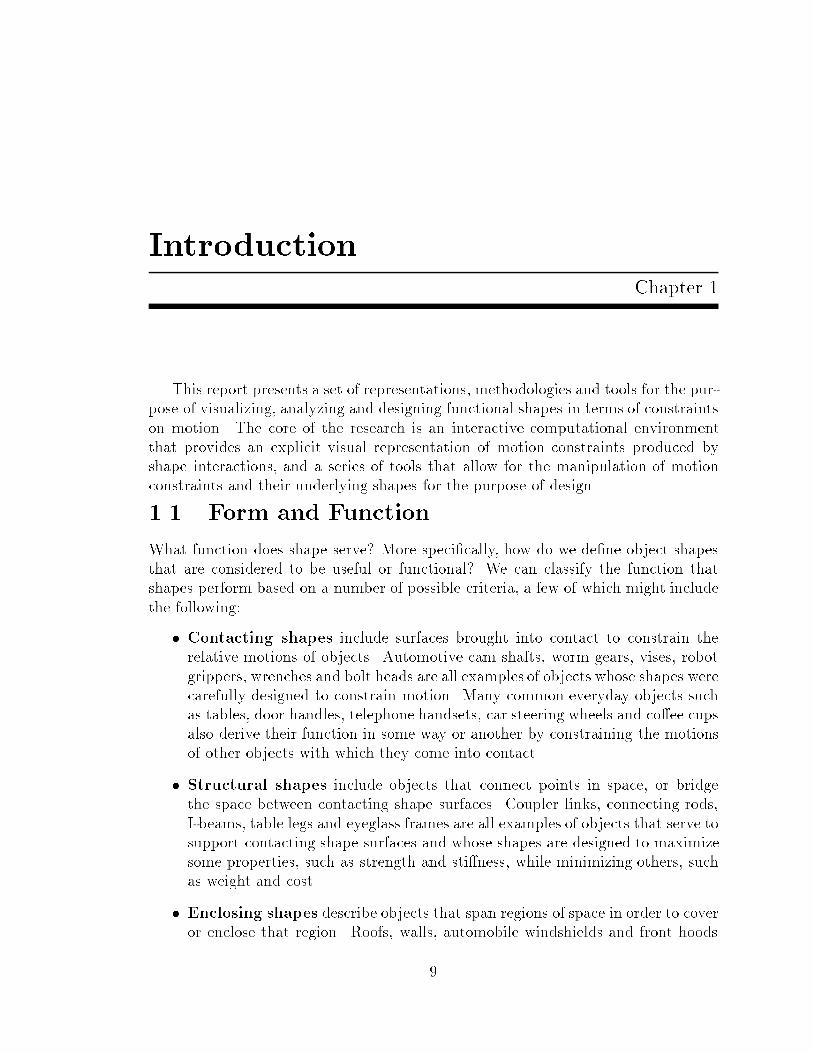
What function does shape serve� More speci�cally� how do we de�ne object shapesthat are considered to be useful or functional� We can classify the function thatshapes perform based on a number of possible criteria� a few of which might includethe following�
� Contacting shapes include surfaces brought into contact to constrain therelative motions of objects� Automotive cam shafts� worm gears� vises� robotgrippers� wrenches and bolt heads are all examples of objects whose shapes werecarefully designed to constrain motion� Many common everyday objects suchas tables� door handles� telephone handsets� car steering wheels and co�ee cupsalso derive their function in some way or another by constraining the motionsof other objects with which they come into contact�
� Structural shapes include objects that connect points in space� or bridgethe space between contacting shape surfaces� Coupler links� connecting rods�I�beams� table legs and eyeglass frames are all examples of objects that serve tosupport contacting shape surfaces and whose shapes are designed to maximizesome properties� such as strength and sti�ness� while minimizing others� suchas weight and cost�
� Enclosing shapes describe objects that span regions of space in order to coveror enclose that region� Roofs� walls� automobile windshields and front hoods
�
� Chapter �� Introduction
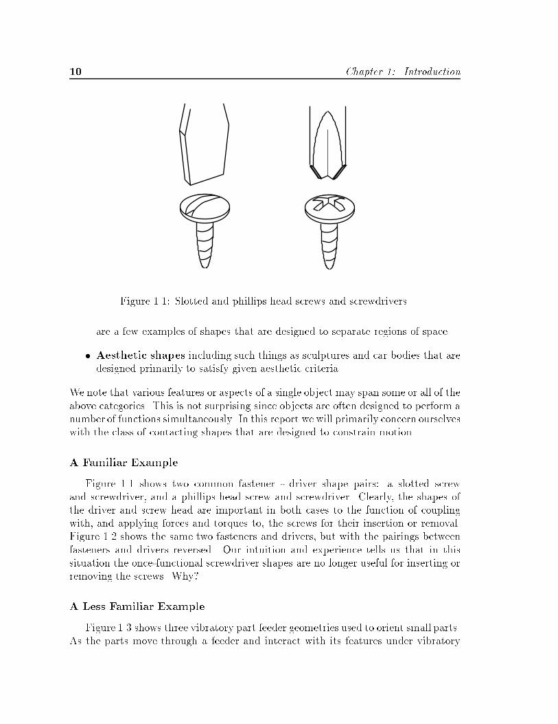
Figure ���� Slotted and phillips head screws and screwdrivers�
are a few examples of shapes that are designed to separate regions of space�
� Aesthetic shapes including such things as sculptures and car bodies that aredesigned primarily to satisfy given aesthetic criteria�
We note that various features or aspects of a single object may span some or all of theabove categories� This is not surprising since objects are often designed to perform anumber of functions simultaneously� In this report we will primarily concern ourselveswith the class of contacting shapes that are designed to constrain motion�
A Familiar Example
Figure ��� shows two common fastener � driver shape pairs� a slotted screwand screwdriver� and a phillips head screw and screwdriver� Clearly� the shapes ofthe driver and screw head are important in both cases to the function of couplingwith� and applying forces and torques to� the screws for their insertion or removal�Figure ��� shows the same two fasteners and drivers� but with the pairings betweenfasteners and drivers reversed� Our intuition and experience tells us that in thissituation the once�functional screwdriver shapes are no longer useful for inserting orremoving the screws� Why�
A Less Familiar Example
Figure ��� shows three vibratory part feeder geometries used to orient small parts�As the parts move through a feeder and interact with its features under vibratory

���� Form and Function ��
Figure ���� Slotted and phillips head screws paired with phillips and slotted screw�drivers�
motion� parts in all but one desired orientation fall out of the feeder to the side� whilethose parts in the desired orientation are allowed to pass through to be picked up by arobot�� The interesting thing to note about the three feeders in Figure ��� is that thegeometrically similar tracks in a� and b� are functionally quite di�erent� whereasthe dissimilar tracks in a� and c� are functionally equivalent� Speci�cally� thefeeder track shown in a� outputs the el�shaped part shown in only one orientation�whereas all other orientations of the part will be knocked o� the track and fall backinto the bowl� The track shown in b�� however� although only slightly di�erent fromtrack a� will output parts in two possible orientations and is therefore unacceptablefor automated assembly� Finally� the feeder track shown in Figure ��� c� will onlyoutput parts in the same orientation as track a�� and hence is functionally equivalentto a��
In the �rst two example feeders a� and b�� one pairing of geometries performsa useful function� while another pairing of apparently similar geometries fails toperform the same intended function� Similarly� in the second and third two examplefeeders b� and c�� quite dissimilar geometries perform the same function� Why�
More speci�cally�
� Why does one pairing of shapes exhibit the desired functional characteristicswhile the other pairing does not�
� What are the important characteristics that determine the functionality of a
�The detailed characteristics of feeder construction and operation are given in Section ����

�� Chapter �� Introduction
(a)
(b)
(c)
Figure ���� Three vibratory parts feeder geometries designed to orient the partsshown� Under given vibratory motion� feeder a� succeeds in orienting the parts�whereas the geometrically similar feeder in b� does not� The very dissimilar feedergeometry in c�� possesses the same feeding function as feeder a��
���� Shape and Motion Constraints ��
given set of shapes�
� How would one go about designing shapes� or modifying an existing shape� toperform a desired function�
This report will address these and related questions�The previous examples were chosen to highlight a number of important points
about shape and function� First� the fastener example illustrates the observation thatthe functionality of object shapes is derived from shape interactions and not fromindividual shapes alone� Functional shapes become essentially useless when they wereused outside the context of their intended interaction with other functional shapes�Second� the feeder example illustrates that our intuition about the function of shapedepends to a large extent on our degree of familiarity with the problem domain�Like the fastener�driver example in Figures ��� and ���� the shapes of the feedersand the parts are clearly important to the function of orienting the parts� However�the precise role that the various shapes play in the stated function is less clear sincethe domain is less familiar� Because our intuition about the functional role of shapeinteractions is rather brittle outside of simple and familiar domains� we are less ableto make appropriate design decisions� As a result� a task such as vibratory feederdesign requires a considerable amount of trial and error� and is considered somethingof a �black art��
��� Shape and Motion Constraints
Let us focus our discussion of function derived from form in the previous section toone of motion constraints derived from shape� Recall the vibratory feeders shownin Figure ���� Although su�cient for a basic understanding of feeder function� thebrief description given of how a vibratory bowl feeder works doesn�t tell us �a� ifa particular feeder example will work� or �b� how to go about designing a feeder�Clearly we need a more precise description of the constraints imposed by interactionsbetween shapes � we need a model of motion constraints�
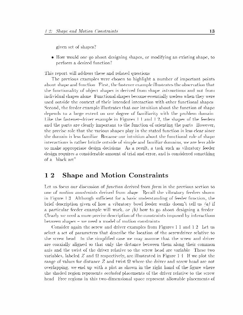
Consider again the screw and driver examples from Figures ��� and ���� Let usselect a set of parameters that describe the location of the screwdriver relative tothe screw head� In the simpli�ed case we may assume that the screw and driverare coaxially aligned so that only the distance between them along their commonaxis and the twist of the driver relative to the screw head are variable� These twovariables� labeled Z and � respectively� are illustrated in Figure ��� If we plot therange of values for distance Z and twist � where the driver and screw head are notoverlapping� we end up with a plot as shown in the right hand of the �gure wherethe shaded region represents occluded placements of the driver relative to the screwhead� Free regions in this two�dimensional space represent allowable placements of

�� Chapter �� Introduction
Z
Θ
Θ
Z
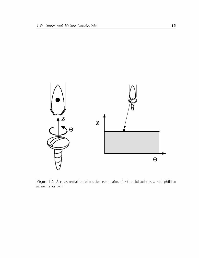
Figure ��� A representation of motion constraints for the slotted screw and screw�driver pair�
���� Shape and Motion Constraints ��
Z
Θ
Θ
Z
Figure ���� A representation of motion constraints for the slotted screw and phillipsscrewdriver pair�

�� Chapter �� Introduction
the driver relative to the screw� The boundary separating the free and occludedregions represents placements of the driver that are in contact with the screw�
We notice a notch in the occluded region of Figure ��� corresponding to place�ments where the blade of the driver is in the screw head�s slot� If we consider thefunction of the screwdriver to be one of transmitting torque to the screw head� thenwe can represent this function in terms of the motion constraints between the driverand screw head as captured by the contact boundaries in Figure ��� Speci�cally� ifwe consider the driver to be represented as the location of a selected point on thedriver in the two�dimensional �Z��� motion constraint diagram of Figure ��� thenthe only way to twist the screw head is to �push� against one of the two vertical sidesof the notch in the � direction� Pushing in the �� direction corresponds to applyinga clockwise torque to the screw� and pushing in the �� direction is equivalent to acounter�clockwise torque applied to the screw��
The capacity of the above representation to capture the function of the screw�driver interaction is further illustrated by the motion constraint diagram for theslotted screw�phillips driver pairing shown in Figure ���� Here the characteristicnotch� whose sides provided the constraint surfaces on which the driver could acton the screw� is missing� As expected� this screw�driver pairing does not exhibitthe desired functionality of allowing torque to be transmitted from the driver to thescrew�
In addition to extracting the function inherent in existing shape interactions� weare also interested in generating contacting shapes with desired functional character�istics� For example� in the case of the slotted screw�driver interaction of Figure ���assume that we wish to be able to drive the fastener into a workpiece� but thatwe don�t want the fastener to be removable� Figure ��� shows a motion constraintdiagram with the desired properties� where the right side of the constraining notchhas been sloped as shown so that the �Z��� point representing the driver will slidealong the constraint boundary and out of the notch rather than allow a torque tobe applied to the screw� The corresponding �one�way� screw head shape shownmight be generated from the new motion constraints by� for example� sweeping thescrewdriver blade along the boundary of the motion diagram� This proposed shapesynthesis process is complicated by the fact that inverting shapes is not unique� Forexample� rather than using the motion constraints in Figure ��� to produce a one�way screw� we could just have easily ended up with a one�way screwdriver� as shownin Figure �� �
�We are treating the relationship between forces and torques somewhat super�cially at this level�Section ����� will address these issues in more detail�

���� Shape and Motion Constraints ��
Z
Θ
Θ
Z
Figure ���� The �one way screw�� one possible instantiation of a modi�ed set ofmotion constraints�

�� Chapter �� Introduction
Z
Θ
Θ
Z
Figure �� � The �one way screwdriver�� another possible instantiation of a modi�edset of motion constraints�
���� Shape and Motion Constraints ��
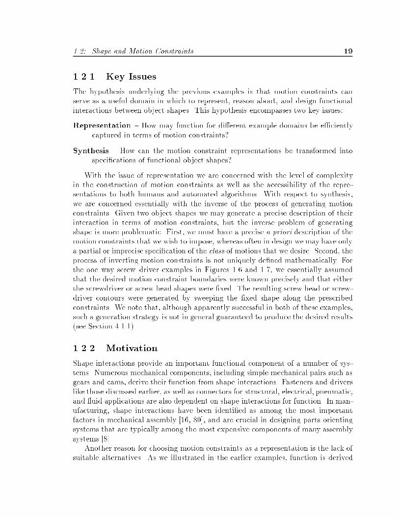
����� Key Issues
The hypothesis underlying the previous examples is that motion constraints canserve as a useful domain in which to represent� reason about� and design functionalinteractions between object shapes� This hypothesis encompasses two key issues�
Representation � How may function for di�erent example domains be e�cientlycaptured in terms of motion constraints�
Synthesis � How can the motion constraint representations be transformed intospeci�cations of functional object shapes�
With the issue of representation we are concerned with the level of complexityin the construction of motion constraints as well as the accessibility of the repre�sentations to both humans and automated algorithms� With respect to synthesis�we are concerned essentially with the inverse of the process of generating motionconstraints� Given two object shapes we may generate a precise description of theirinteraction in terms of motion constraints� but the inverse problem of generatingshape is more problematic� First� we must have a precise a priori description of themotion constraints that we wish to impose� whereas often in design we may have onlya partial or imprecise speci�cation of the class of motions that we desire� Second� theprocess of inverting motion constraints is not uniquely de�ned mathematically� Forthe one way screw�driver examples in Figures ��� and �� � we essentially assumedthat the desired motion constraint boundaries were known precisely and that eitherthe screwdriver or screw head shapes were �xed� The resulting screw head or screw�driver contours were generated by sweeping the �xed shape along the prescribedconstraints� We note that� although apparently successful in both of these examples�such a generation strategy is not in general guaranteed to produce the desired results�see Section ������
����� Motivation
Shape interactions provide an important functional component of a number of sys�tems� Numerous mechanical components� including simple mechanical pairs such asgears and cams� derive their function from shape interactions� Fasteners and driverslike those discussed earlier� as well as connectors for structural� electrical� pneumatic�and �uid applications are also dependent on shape interactions for function� In man�ufacturing� shape interactions have been identi�ed as among the most importantfactors in mechanical assembly ���� ��� and are crucial in designing parts orientingsystems that are typically among the most expensive components of many assemblysystems ����
Another reason for choosing motion constraints as a representation is the lack ofsuitable alternatives� As we illustrated in the earlier examples� function is derived
� Chapter �� Introduction
explicitly from the shape interactions that constrain motion� Most existing designtools� such as Computer Aided Design �CAD� systems� focus on modeling the geome�try of individual components in isolation� Individual shapes are considered explicitly�but any potential shape interactions are� for the most part� implicit in the geometricalrepresentation� Consideration of shape interactions in such systems� if present at all�is usually limited to checking for interference between parts undergoing prescribedmotions� typically along or around �xed axes� Interference checking� however� doesnot capture the potential functionality of object shapes for constraining motion� Forsome specialized applications� attempts have been made to divide individual objectshapes into equivalence classes� As we saw in the part�feeder examples of Figure ����however� similarity in shape does not necessarily correspond to similarity in function�
Shape design based on motion constraints is presently practiced for a limited setof well de�ned �xed�axis mechanisms such as cams and gears� In cam design� forexample� the desired motion of a �xed shape cam follower is plotted as a function ofcam rotation� The motion of the follower relative to the cam plate is then used togenerate a tool path for cutting the corresponding cam shape� Similarly� gear pro�lesare often generated directly by hobbing or rolling processes where a �xed cutter shapeis used to generate the complementary gear shape� Both of these processes are similarin concept to the one�way fastener synthesis example in Figure ���� However� fewdesign tools utilizing motion constraints exist for other classes of shape interactions�and none are presently able to deal with non��xed�axis devices� An extensive amountof work has been done in the area of analyzing the motions of mechanisms constructedfrom lower order kinematic pairs �i�e� revolute and prismatic joints�� Techniques tospecify the parameters for such mechanisms� such as link lengths for mechanismsof known topology� have also been developed and incorporated into computer aideddesign tools� However� these techniques are not suitable for more general kinematicinteractions that cannot be characterized only in terms of interconnected links andjoints�
����� Goals and Applications
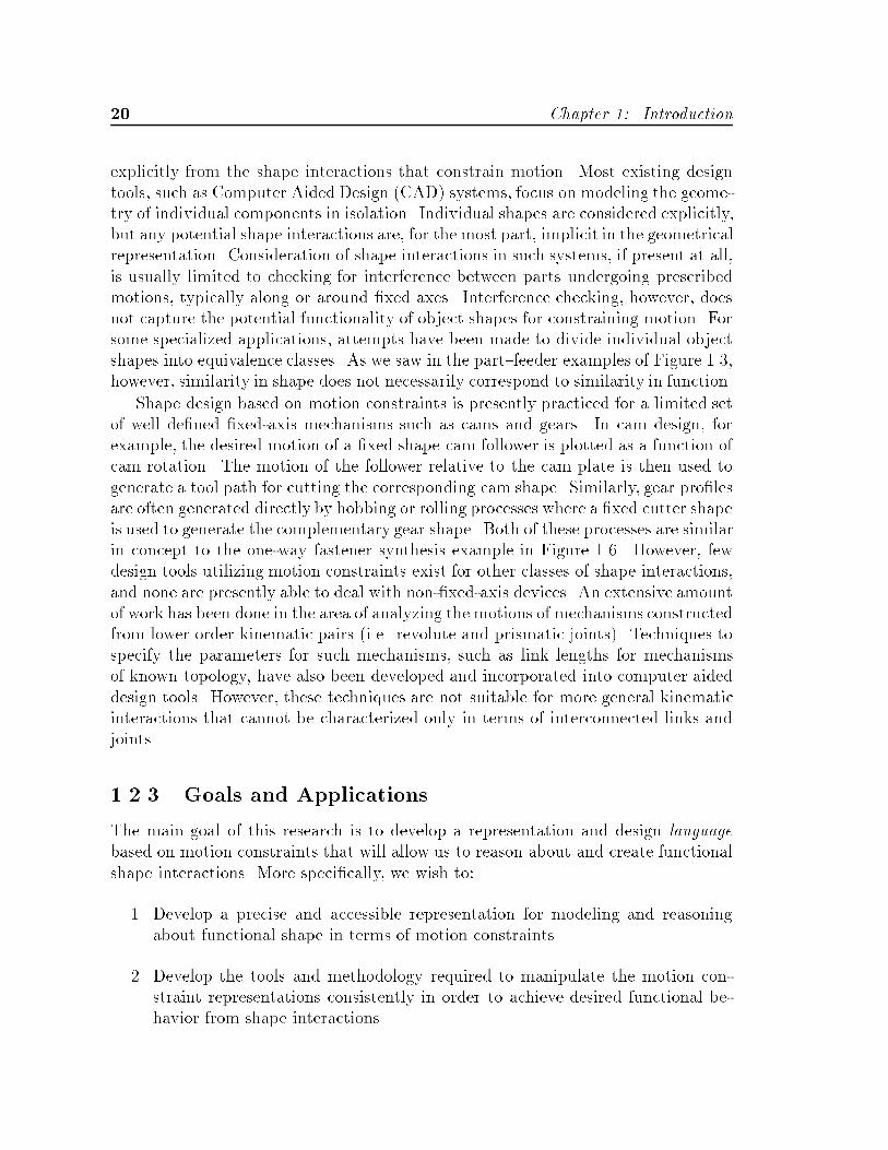
The main goal of this research is to develop a representation and design languagebased on motion constraints that will allow us to reason about and create functionalshape interactions� More speci�cally� we wish to�
�� Develop a precise and accessible representation for modeling and reasoningabout functional shape in terms of motion constraints�
�� Develop the tools and methodology required to manipulate the motion con�straint representations consistently in order to achieve desired functional be�havior from shape interactions�

���� Shape and Motion Constraints ��
Vibratory Bowl Feeders
Fixtures & Pallets
Part Mating
APOS Parts Feeders
Figure ���� Four application domains�
These two sub�goals address directly the key issues of functional representation andsynthesis identi�ed earlier�
In addition to the above goals� we would like to be able to address some of thelimitations of existing representations and techniques mentioned in Section ������In particular� we would like to be able to represent and design more general shapeinteractions �i�e� other than pre�de�ned linkages and pins� revolute and prismaticjoints� and �xed�axis mechanisms�� We also would like to apply the representationsand tools across a range of speci�c application domains in order to determine to whatextent such representations are able to generalize functional characteristics beyondindividual examples� Ideally these representations will enable us to identify or createfunctional shapes that otherwise might not have been generated�
We will judge the motion constraint representations and synthesis tools by thedegree to which they enable us to perform analysis and design within a set of wellde�ned example domains� To do this� we will speci�cally consider four application
�� Chapter �� Introduction
domains� compliant assembly� vibratory bowl feeders� assembly �xtures� and theAPOS vibratory feeding system� Simpli�ed examples of these four domains areshown in Figure ���� The representations and tools developed in this report will beused to analyze and reason about the functional characteristics of examples fromeach of the application domains� and to perform design in the �rst two� We willdiscuss these examples in greater detail in Chapter ��
��� Background and Related Work
This research draws upon work in a number of di�erent �elds� Among the �elds weconsider to be most closely related are�
� Geometrical modeling and kinematics�
� Robot motion planning�
� Qualitative reasoning�
� Design methodology and computer aided engineering�
� Simulation and visualization of physical processes�
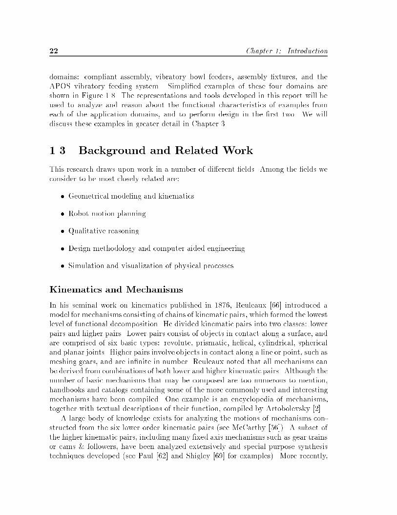
Kinematics and Mechanisms
In his seminal work on kinematics published in �� �� Reuleaux ���� introduced amodel for mechanisms consisting of chains of kinematic pairs� which formed the lowestlevel of functional decomposition� He divided kinematic pairs into two classes� lowerpairs and higher pairs� Lower pairs consist of objects in contact along a surface� andare comprised of six basic types� revolute� prismatic� helical� cylindrical� sphericaland planar joints� Higher pairs involve objects in contact along a line or point� such asmeshing gears� and are in�nite in number� Reuleaux noted that all mechanisms canbe derived from combinations of both lower and higher kinematic pairs� Although thenumber of basic mechanisms that may be composed are too numerous to mention�handbooks and catalogs containing some of the more commonly used and interestingmechanisms have been compiled� One example is an encyclopedia of mechanisms�together with textual descriptions of their function� compiled by Artobolevsky ����
A large body of knowledge exists for analyzing the motions of mechanisms con�structed from the six lower order kinematic pairs �see McCarthy ������ A subset ofthe higher kinematic pairs� including many �xed axis mechanisms such as gear trainsor cams � followers� have been analyzed extensively and special purpose synthesistechniques developed �see Paul ���� and Shigley ���� for examples�� More recently�

���� Background and Related Work ��
computationally based analysis techniques combined with synthesis tools to auto�matically select parameters for mechanisms of �xed topology� such as link lengths�have been developed by a number of researchers �see Bodduluri � McCarthy ����Kramer � �� and Hoeltzel � Chieng ������
Shape Synthesis for Kinematic Pairs
The techniques and design tools described above are limited to the selection andmanipulation of parameters for pre�determined kinematic pair types� Joskowicz �Addanki ��� outline an approach for modifying and generating the shape pro�lesof kinematic pairs from speci�cations of desired input�output motion relationships�Gupta � Jakiela ���� developed a shape design system that takes as input two planarshapes� one of which is �xed� and a functional diagram relating the relative motionof the two objects� As the �xed shape is swept along a prescribed motion path itis used to �carve� out the other object�s shape� analogous to moving a hot knifethrough �computational butter��
Robot Motion Planning
Work in the �eld of robot motion planning has considered numerous aspects of therelationship between shape and motion� Tasks such as �nding a collision free pathfor a robot among obstacles and the automatic synthesis of robot motions from highlevel task speci�cations have been extensively studied� and a number of powerfulrepresentations and analysis tools have been developed�
An important problem identi�ed early on in the development of computer con�trolled manipulators was that of planning a collision free path of a manipulatoramong obstacles� Udupa � � introduced a representation in which the problem ofmoving a robot among obstacles was transformed to an approximately equivalent andsimpler problem of moving a point among transformed obstacles� Lozano�P erez ���formalized this idea by constructing the con�guration space� whose axes are therobot�s degrees of freedom� in which constraints on the robot�s motion due to inter�actions with obstacles in the robot�s environment could be represented directly asconstraints on the motion of the robot� More generally� con�guration space is the pa�rameter space representing the relative locations �including position and orientation�of rigid objects� Although it has been used extensively in robotics and planning tomodel kinematic constraints imposed on the set of legal motions of objects by theirshapes� the underlying idea of using a parameter space analysis has a long history inphysics�

�� Chapter �� Introduction
Construction of Con guration Space
Many algorithms for constructing motion constraint representations in con�gurationspace have been developed for various motion planning and analysis applications� andthe function and performance of these algorithms depends heavily on their intendedapplication� The two primary applications for con�guration space in robotics are theplanning of collision free paths for manipulators and the analysis of the motion of ob�jects in contact� Planning for collision avoidance typically involves searching amongthe free regions between obstacles in con�guration space �see Lozano�P erez ����� Therepresentations and algorithms constructed for this task therefore focus on charac�terizing the free and occluded regions of con�guration space� Con�guration spacerepresentations used for the analysis of motions of objects in contact focus less onthe distinction between free and occluded space and more on the exact nature ofthe boundaries separating the two � the constraint surfaces determined by objectinteractions�
Lozano�P erez ��� developed a simple and e�cient algorithm for computing theboundary of the �x� y� con�guration space obstacle formed by the interaction of twopolygons without rotations� The algorithm is based on ordering the edges from thepolygons by their orientation �measured counterclockwise�� with the resulting listof ordered edges describing the �possibly non�simple� polygon forming the obstacleboundary� Avinaim et� al� ��� developed an exact representation of the full �x� y� ��con�guration space obstacle formed by two interacting polygons� Donald ���� de�veloped and implemented an algorithm for planning collision free paths of threedimensional polyhedra with six degrees of freedom� In his representation� Donalddescribed the �ve�dimensional constraint surfaces �submanifolds� in the completesix�dimensional con�guration space� Bajaj � Kim �� extended the class of mod�eled object shapes beyond polygons by developing algorithms to construct the �x� y�obstacle boundary for two interacting objects represented by segments of algebraiccurves�
To improve the runtime performance of motion planning systems� a number ofresearchers have developed e�cient algorithms to compute approximations for ob�stacles in con�guration space� Lengyel et� al� ��� implemented a real�time motionplanning system for polygonal objects by utilizing existing computer graphics hard�ware �depth bu�er� to rasterize �xed�rotation slices of obstacles in con�gurationspace� Branicky � Newman ���� developed and implemented algorithms to rapidlycompute approximate con�guration space obstacles for multi�link manipulators mov�ing among polyhedral obstacles� Lozano�P erez � O�Donnell ���� utilized a parallelarchitecture computer to rapidly compute and search for paths among obstacles ina six�dimensional con�guration space generated for a six link manipulator� Theyachieved good performance by utilizing inherent symmetries in the structure of con��guration space obstacles for revolute joint manipulators with intersecting axes� in
���� Background and Related Work ��
order to represent and encode the obstacles within a recursive data structure thatmay be quickly computed and searched by massively parallel algorithms� A com�plete task level planning system named Handey� incorporating an implementation ofthe above algorithm in addition to a number of other algorithms addressing variousaspects of robot motion planning� is described in Lozano�P erez� et� al� �����
Sensorless manipulation using task mechanics
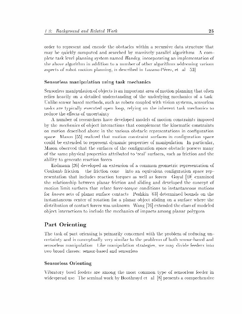
Sensorless manipulation of objects is an important area of motion planning that oftenrelies heavily on a detailed understanding of the underlying mechanics of a task�Unlike sensor based methods� such as robots coupled with vision systems� sensorlesstasks are typically executed open loop� relying on the inherent task mechanics toreduce the e�ects of uncertainty�
A number of researchers have developed models of motion constraints imposedby the mechanics of object interactions that complement the kinematic constraintson motion described above in the various obstacle representations in con�gurationspace� Mason ���� realized that motion constraint surfaces in con�guration spacecould be extended to represent dynamic properties of manipulation� In particular�Mason observed that the surfaces of the con�guration space obstacle possess manyof the same physical properties attributed to !real� surfaces� such as friction and theability to generate reaction forces�
Erdmann ���� developed an extension of a common geometric representation ofCoulomb friction � the friction cone � into an equivalent con�guration space rep�resentation that includes reaction torques as well as forces� Goyal �� examinedthe relationship between planar friction and sliding and developed the concept ofmotion limit surfaces that relate force�torque conditions to instantaneous motionsfor known sets of planar surface contacts� Peshkin ���� determined bounds on theinstantaneous center of rotation for a planar object sliding on a surface where thedistribution of contact forces was unknown� Wang � �� extended the class of modeledobject interactions to include the mechanics of impacts among planar polygons�
Part Orienting
The task of part orienting is primarily concerned with the problem of reducing un�certainty and is conceptually very similar to the problems of both sensor�based andsensorless manipulation� Like manipulation strategies� we may divide feeders intotwo broad classes� sensor�based and sensorless�
Sensorless Orienting
Vibratory bowl feeders are among the most common type of sensorless feeder inwidespread use� The seminal work by Boothroyd et� al� ��� presents a comprehensive

�� Chapter �� Introduction
and in depth analysis of feeding and orienting techniques in general� and in particularbowl feeders� They conducted numerous experiments to determine the probabilitydistribution for the resting aspects of parts and developed techniques to computethe throughput e�ciency of vibratory bowl feeder systems� The main result of thiswork is a handbook of feeders indexed by a taxonomy of basic part geometries� Thishandbook serves as an essential tool for designers and manufacturing engineers inmaking an initial selection of feeder types and geometries appropriate for a given setof parts�
The APOS� �Advanced Parts Orienting System� developed by Sony and de�scribed by Shirai � Saito � � represents a simple and e�cient hardware implemen�tation of vibratory feeding that combines reusable system hardware with integratedpalletizing and part transport� APOS has been successfully applied in a wide vari�ety of manufacturing systems both inside and outside Sony� The primary challengein using the system is the initial design of pallets that capture� sort� and hold partsfor assembly � hence its interest to us in the context of shape design from motionconstraints� Moncevicz ���� describes an interesting approach that seeks to furtherintegrate orienting and assembly operations� It is based on a modi�cation to thebasic APOS system in which component parts are both oriented and assembled invibratory pallets where the pallets are themselves subassemblies� an approach theyrefer to as �shake�n make� assembly� In another interesting approach� Singer � Seer�ing � �� distinguish and separate part orientations using di�erences in the dynamicproperties of parts by running the parts over a small fence placed across a movingtrack�
Part Orienting in the Context of Planning
Natarajan ���� considered a number of general theoretical and computational aspectsof part orienting as a sensorless manipulation task� Erdmann �Mason �� � developedand implemented an algorithm to generate sequences of sensorless tray tilting motionsdesigned to place a randomly oriented part into one corner of the tray in a knownorientation� Goldberg ��� developed algorithms to generate sequences of planargrasps using a frictionless parallel jaw gripper to orient a polygonal part of knownshape in the plane� Although a robot was used to perform the grasping motions� nosensing was done�
Sensor�Based Orienting
Numerous systems consisting of combinations of robots� cameras� lasers� photodiodes�contact switches� actuators� etc� have been developed and implemented� Gordon ����provides both a good example of an integrated closed loop orienting and assemblysystem using a laser� vision system and a robot� as well as an excellent survey ofrelated sensing and orienting techniques�

���� Background and Related Work ��
Qualitative Reasoning
Work in the �eld of automated qualitative reasoning has examined the relationshipbetween the shape of kinematic pairs and their corresponding function with the goalof extracting abstract descriptions of function from form� Faltings ���� introduced theplace vocabulary� an abstraction for mechanism function derived from the topologyof free regions in the con�guration spaces of the kinematic pairs composing themechanism� A place vocabulary consists of a graph representation in which boundedfree regions in con�guration space are represented as nodes and connections betweenthe regions as arcs� The resulting graph structure embeds a compact encoding forthe topology of free regions in con�guration space that may be parsed to obtain thefunctional attributes of the underlying mechanism�
Joskowicz �� also uses boundaries and regions in the con�guration space of amechanism to perform qualitative analysis of mechanism behavior� In addition� heintroduced a heuristic algorithm for designing the shapes of mechanism componentsfrom descriptions of desired behavior represented either in terms of con�gurationspace maps or functional relationships between the input and output parametersde�ning the mechanism�s con�guration space� Joskowicz � Sachs ��� extended andimplemented this work on kinematic constraints to include the dynamic behavior ofmechanisms� One result is a system for the automated modeling and analysis of pla�nar mechanisms consisting of chained kinematic pairs� The system �rst constructsthe �D con�guration space for each kinematic pair in the mechanism and then auto�matically explores both the dynamic and kinematic behavior in each of the coupledcon�guration space regions�
Bourne et� al� ��� used con�guration space as a domain for examining the rela�tionship between machining tolerances for parts and the functionality of those partsin a mechanism� Speci�cally� they searched for parametric variations that changedthe topology of free space regions in a mechanism�s con�guration space in order toboth highlight sensitive design parameters and to derive tolerance constraints thatwere related directly to the intended function of a given mechanism�
Design Methodology
Nevins � Whitney ��� present an overview and series of detailed case studies on thedevelopment and implementation of concurrent design strategies for products andprocesses� The broad aim of concurrent engineering is to consider multiple aspectsof and constraints on a product�s function� manufacture� use and �recently� disposalas early on in the design process as possible�
One area of concurrent design dealing with product assembly is design for as�sembly �DFA�� extensively developed by Boothroyd and others � �� DFA method�ologies consist of case studies� design rules and heuristics aimed at reducing the

�� Chapter �� Introduction
overall number of component parts and fasteners in a product�s design� as well asmaking the parts easier to identify and orient� Jakiela ��� implemented a designenvironment that utilized encoded design for assembly �DFA� rules to make sug�gestions for changes to the input geometry during the design session� Whitney et�al� ��� presented detailed models� analyses and experiments on the performance ofvarious chamfer pro�les during the one�point contact phase of peg�in�hole assembly�Caine ���� examined the e�ect of a number of chamfer pro�les on the jamming andwedging characteristics of planar peg�in�hole assembly during two�point contact� DeFazio et� al� ���� have implemented a feature based interactive CAD environmentfor analyzing the assemblability of parts using a graph of liaison diagrams encodingthe desired relationships between collections of parts in order to select the properassembly sequence�
Simulation and Visualization
The primary roles of simulation in design is that of model veri�cation and trou�bleshooting via exploration of the functional properties of the system under consid�eration� One of the di�culties frequently encountered in simulation involves inher�ently discontinuous phenomenon� such as impacts� that result in constantly changingboundary conditions that require frequent changes to the system models�
Gilmore � Streit ���� developed a system for predicting motion under multiplediscontinuous contacts using a rule based algorithm that determines changes to con�straints and automatically reformulates the dynamical equations accordingly� Thesystem was applied to the analysis of a parts feeder for planar parts consisting of asequence of angled fences� Donald � Pai ��� utilized a simpli�ed con�guration spacerepresentation to analyze and simulate the motion of rigid planar parts with compli�antly connected �snap� features moving in a plane� The resulting system was usedto help redesign the shape of the interacting planar parts for more reliable assembly�
Simulation techniques have also been applied in interactive graphical environ�ments� Witkin � � introduced a reformulation of dynamical and constraint equa�tions describing a system so that constraints could be rapidly added and removedas the equations were integrated numerically� In one application of this technique�graphical entities could be created� linked and unlinked interactively in real timeby a user� Related techniques developed in the rapidly evolving visualization �eldhave found application in such diverse �elds as computational �uid mechanics� me�teorology� resource extraction� and computational biology �see Patrikalakis ���� fornumerous examples�� In all cases� the basic goal of such technology is to representcomplex or large sets of data within a uni�ed representation that aids in reasoningabout and manipulating the data�

���� Background and Related Work ��
Particularly Relevant Work
In his Ph�D� thesis� Brost ���� developed and implemented an exact representation forthe �x� y� �� con�guration space obstacle formed by two interacting polygons� Unlikecollision�free planning applications� Brost�s implementation focuses on constructing adetailed motion constraint representation� including the mechanics of object contact�that is suitable for the detailed analysis and planning of object interactions� Inaddition to kinematic constraints between planar objects� Brost developed a series ofalgorithms for computing regions of possible static equilibrium and bounded regionsde�ning con�gurations reachable from initial positions in the presence of positionaland control uncertainty� Brost applied these algorithms to the tasks of analyzingand planning robot pushing motions and dropping of parts into orienting �xtures�
The representations and implementation developed by Brost preceded those pre�sented in this report� and there a number of similarities and di�erences between thetwo� Similarities between the two implementations include�
� Both implementations consider interactions among objects modeled as poly�gons moving in the plane with three degrees of freedom��
� Both implementations compute an exact representation of the kinematic mo�tion constraint surfaces� represented in �x� y� �� con�guration space� producedby planar polygon interactions�
� Both implementations model the mechanics of object interactions� includingcoulomb friction�
The primary objective of Brost�s implementation is the automatic constructionof plans� consisting of either pushing or dropping motions� represented geometricallyas regions in con�guration space backprojected from speci�ed goal states� This isin contrast to the forward projections from speci�ed starting positions�regions thatare computed by cspace�shell for the purpose of visualization and analysis by a user�Some of the speci�c di�erences between Brost�s implementation and the cspace�shellimplementation presented in this report include�
� Brost treats the shapes of objects as static variables since he is concerned withplanning motions for objects of known shape� In cspace�shell� however� it is themodi�cation of object shapes that is of primary concern� As a result� Brost�simplementation precomputes the full topology of the con�guration space ob�stacle whereas� for reasons of computational speed� cspace�shell computes anddisplays the complete set of individual contact facets� but only computes the
�Brost�s algorithms implicitly consider both polygons to be fully supported by an underlyingplanar surface� Hence there is no explicit consideration of limited support due to interactions witha non�in�nite supporting plane pro�le as with the track in the bowl feeder examples in this report�

� Chapter �� Introduction
local topology �facet adjacencies and intersections� that a�ects the integratedmotion paths�
� Brost explicitly considers and models uncertainty in his representations andalgorithms� both symbolically and numerically� in order to compute motionplans that are robust� The present implementation of cspace�shell performsonly exact numerical computations�
The following is a comparison between speci�c components Brost�s implementa�tion �highlighted� and cspace�shell�
CO� produces an exact metric and topological description of the �x� y� �� kinematicmotion constraints for two input polygons� It is comparable to the facet gener�ation and �local� topological checking performed during motion integration incspace�shell� However� as mentioned above� cspace�shell does not precomputethe full topology of the con�guration space obstacle� which Brost�s implemen�tation must do in order to perform backprojection computations�
STATIC� computes and labels regions on the surface of the motion constraint setthat may correspond to static equilibrium under speci�ed applied forces anduncertainty� There is nothing directly comparable in cspace�shell� althoughstatic equilibrium �without uncertainty� is checked during motion integrationin order to detect motion termination�
BPe� produces energy �puddles� on the surface of the motion constraint set thatde�ne the set of initial positions �and orientations� from which an object maybe dropped in a gravity �eld and still be guaranteed to come to rest in aspeci�ed location� These energy puddles are equivalent to the conservativeenergy bounded forward projections described in Section ���� with e " �� Twoimportant di�erences are that BPe is at least partially implemented and thatthe resulting regions are backprojected� i�e� are generated backwards fromdesired goal states� The energy bounded forward projections in this reporthave not been implemented�
BPi� computes backprojected regions by expanding the set of points on the surfaceof the con�guration space obstacle from which a desired goal will be reached�The resulting surface regions are then lifted from the surface in order to formvolumes in con�guration space that de�ne the set of initial positions �andorientations� from which an object may be reliably pushed into a speci�edlocation in the presence of uncertainty� BPi is similar to� but signi�cantlymore general than� the numerically integrated forward projections computedby cspace�shell� In addition� BPi can model higher order dynamics whereasthe present implementation of cspace�shell assumes only quasi�static motions�

��� Contributions of the Research ��
Another piece of work particularly relevant to this research was described in anunpublished research memo by Lozano�P erez ����� who proposed both a represen�tation of function from shape in terms of motion constraints� and the view of theprocess of shape design as an inverse of the motion planning problem� He also sug�gested vibratory bowl feeder design as a promising domain in which to develop andtest these ideas�
Speci�cally� Lozano�P erez proposed a design model in which feeder motions werecharacterized and classi�ed into a basic set of primitive motions� These primitivemotions would serve as a vocabulary with which the desired motions of parts to beoriented could be concisely represented� To generate feeder geometries� characteristicmotion paths would be composed from this vocabulary and parts would be sweptalong those paths� e�ectively cutting out the desired feeder� As we will see in Chap�ter � the geometries generated by such swept motions provide the necessary butnot the su�cient conditions to guarantee that the desired motions will be achieved�Although these ideas were not developed further or implemented by Lozano�P erez�they provided the inspiration and underlying conceptual framework that guided thebulk of the work described in this report�
��� Contributions of the Research
The contributions of this research lie both in the underlying concept of using motionconstraints as a paradigm for shape design� and in the representations and toolsdeveloped for this purpose� The major contributions of this research include�
� Motion Constraint Based Techniques for the Design of FunctionalShapes� This research has demonstrated that motion constraints may beused as the basis for design of functional shapes as well as for the analysis offunctional shapes�
� Functional Constraint Representations� We have developed mathemati�cally precise and computationally accessible functional representations in termsof motion constraints for the four application domains shown in Figure ����compliant assembly of rigid parts� vibratory bowl feeders� part �xtures� andAPOS vibratory parts feeders�
� Design Tools and Methodologies for Generating Functional ShapeInteractions� We developed and implemented a set of tools and methodologiesapplicable to the design of vibratory bowl feeders and compliant assemblies�
� Computation of Planar Support� We developed an e�cient algorithm forcomputing the condition of support for an object by a planar support surfaceunder the e�ects of gravity�

�� Chapter �� Introduction
� Lower Dimensional Mappings of Transitions to Higher DimensionalMotions� We developed a representation that maps the transition from lowerd�o�f� constrained motions to higher d�o�f� motions as a result of changes inplanar support� This mapping allowed the essential characteristics of complexobject motion to be captured within a simpler representation�
� Interactive Computational Environment for Functional Shape De�sign� We developed and implemented an interactive computational environ�ment for shape design based on a �near� real�timemotion constraint generation�visualization and manipulation tool� This system also demonstrated that thecomputation of constraints in con�guration space� for objects with three de�grees of freedom� may be computed quickly for planar objects of �moderate�complexity�
� Functional Shape Generation by Means of Swept Motions Doesn�tWork� We illustrated that shape generation techniques based on swept motionof �xed shape objects are not guaranteed to provide the intended motion con�straints� illustrating the need for a more accurate and complete representationfor analyzing and synthesizing shape interactions�
� Dynamic Visualization of Coupling Between Motion Constraints andShape Parameters� We utilized the above computational environment to vi�sualize� identify� and interactively explore the dynamic nature of constraintcoupling� We introduced the notion of dynamic constraint visualization as ameans of examining the neighborhood of a point in design space and high�lighting the inherent limitations and constraints on achieving a desired set offunctional properties�
��� Outline of the Report
Chapter � develops the detailed motion constraint representations for the class ofobjects that may be modeled as planar polygons with a maximum of three degreesof freedom �two translational� one rotational�� The notion of motion constraints isextended to include both kinematic and non�kinematic constraints� and various typesof motion forward projection are developed for various mechanics models�
Chapter � develops the four application domains introduced in Figure ���� com�pliant assembly� vibratory bowl feeders� assembly �xtures� and the APOS vibratoryfeeding system� The motion constraint representations developed in Chapter � aredisplayed in visual form and used to analyze and reason about the functional char�acteristics of examples from each of the application domains�
Chapter extends the utility of the representations developed in Chapter � byintroducing a series of tools to manipulate the motion constraints directly together

��� Outline of the Report ��
with their underlying shapes� These tools are applied to the design of a set of func�tional shapes from two of the example domains introduced in Chapter �� compliantassembly and vibratory bowl feeders� Methodologies are developed to address theinherent coupling and complexity of design in the two application domains�
Chapter � describes the implementation of the motion constraint representationsand design tools on a graphics workstation� The major components of the implemen�tation are outlined and discussed� and a number of optimizations required to generateand interactively manipulate motion constraints in near real�time are highlighted�
Chapter � summarizes the major concepts of the research and a discussion of thecurrent limitations and possible future extensions of the approach�
Appendix A contains derivations of the models used to compute forward projec�tion bounds for an object dropped from rest in a gravity �eld� and a conservativeestimate of the maximum vertical height that may be reached by an object bouncingin contact with a vibrating table� Appendix B contains derivations of the curvatureof contact facets along a curve on the surface of the facet� which are used to ensureaccuracy bounds on the numerical path integration� Appendix C presents the pri�mary data structures used in the implementation of the motion constraint analysisand design system�

�� Chapter �� Introduction
Representing Function
Chapter �
In this chapter we will develop the representations necessary to capture functionin terms of motion constraints� These representations will provide the foundationupon which we will evaluate and manipulate both shape and other parameters asnecessary to achieve desired functional characteristics�
��� Functional Motion Constraints
Precise Representations of Motion Constraints
We often use terms such as guide� support and restrain in describing the functionsperformed by interactions between shapes� These terms are used to refer to con�straints on speci�c subclasses of motions that are qualitatively distinct with respectto the intended function of the constraint� Unfortunately� the meaning of the termconstrain in the context of one example may be di�erent in another� or equivalentto the meaning of support in yet another� Clearly the semantics of the above wordsare too vague and imprecise representation to be suitable for accurately character�izing function� What we need is a more precise representation# a model for functionrepresented in terms of motion constraints�
Consider again the fastener and driver examples in Section ���� In describingthe function embodied in the fastener�driver interactions in Figures �� and ���� weadopted a representation based on the space of parameters describing relative objectpositions� The shaded regions illustrated in these �gures represented driver positionsthat were unreachable due to the presence of the screw head� and the boundariesbetween shaded �occluded� and unshaded �free� regions represented kinematic con�straints on the object motions due to contact interactions between their shapes�Looking at these boundaries another way� we may view them as constraining whereone object can and cannot go relative to another�
��

�� Chapter �� Representing Function
Kinematic and Non�Kinematic Motion Constraints
Is the above representation for kinematic motion constraints su�cient to capturefunction� Consider the example of a cup sitting on a table� We can say that theinteraction between the shape of the cup and the table constrains the cup to remainon or above the table�s surface� Expressed in a space representing the position andorientation of the cup relative to the table� similar to that used for the fastener�driverexamples� the point representing the con�guration of the cup may placed anywhere inthe free region bounded by the constraint surfaces formed by the interaction betweenthe cup and table� But what if we now wish to answer the question �does the tablesupport the cup�� Clearly this representation alone is not su�cient to determine thebehavior of such a system� What�s missing is an additional set of non�kinematicmotion constraints that� when combined with the kinematic motion constraints� willtell us not only where an object can and cannot go� but where it will go under givenconditions�
��� A Parameter Space for Motions
We represent the position of one object relative to another object as a transformationbetween coordinate frames attached to those objects� The parameters used to de�nethis transformation are the parameters that will be used to express a relative motionbetween the objects� These con�guration parameters� which may include translationsas well as rotations� are used to de�ne a space in which object positions are given aspoints and object motions by trajectories � a con�guration space� We may considerthe con�guration space a form of kinematic state space for representing motionsthat is a direct analogy to the generalized phase space used to describe the behaviorof a second order dynamical system � without the velocity information� For manyapplications we may furthermore assume one of a pair of interacting objects to be�xed in a global reference frame so that the relative position of the moving objectbecomes a speci�cation of absolute position�
Con�guration space is a natural choice for our application as it allows us to rep�resent both motions and constraints on motions with the same set of variables� Aswe shall see� shapes will be combined via contact interactions to form an explicit rep�resentation of motion constraint� while the shapes themselves remain implicit withinthe resulting representation� The dimensionality of the con�guration space will de�pend on the number of parameters necessary to describe any possible object motion#the maximum number of degrees of freedom of the system under consideration� Thenumber of degrees of freedom for general motions of individual three dimensionalobjects� and hence the number of dimensions of the con�guration space� will be six�three translational parameters and three rotational parameters�
Reducing the degrees of freedom for an object is desirable both in terms of the

���� Kinematic Constraints ��
number of parameters that must be considered and the complexity of the analysisthat must be performed� From the standpoint of human visualization of function�three dimensions is the realistic limit within which our spatial reasoning abilitieswill be useful in understanding motions and constraints represented in con�gurationspace� Furthermore� the complexity of computing constraints in con�guration spacegrows polynomially with the geometric size of the objects� and exponentially with thedegrees of freedom �see Canny ������
Fortunately� it will often be su�cient to consider only a subset of the possiblemotions of an object for a particular task� In some cases� symmetry will allow us toremove degrees of freedom that might be considered redundant# axisymmetric objectssuch as a cylindrical peg in hole modeled as planar objects is an example of one suchcase� In other cases the motions of objects may initially be constrained enoughto require further consideration of only the remaining degrees of freedom� such asan object dropped onto a table that then slides across the table surface �withouttipping�� And in still other cases� object motions may be constrained by design fromthe outset� such as gears and cams rotating about �xed axes or pistons sliding withincylinders� Finally� for those domains where more than three degrees of freedom mustbe considered� it is often possible to subdivide or otherwise isolate di�erent aspectsof function that individually may constitute fewer degrees of freedom� For example�by considering the motion of an object sliding in the plane that may tip as a series ofsub�motions consisting of purely planar motions connected by tipping motions� wetradeo� simpler models in return for a greater number of those models that must begenerated� We will consider a number of such simpli�cations later on in this chapter�
For most of this report we will consider in detail objects constrained to have threeor fewer degrees of freedom� Speci�cally� we will model and analyze in detail objectsthat move only within a plane� Motions will consist of displacements in x and y of areference point attached to the moving object� and a rotation in � of the object abouta normal to the plane of motion� We will occasionally refer to the three dimensionalcon�guration space described by these parameters as ���D �R� � SO���� in orderto distinguish it from �D �R���
��� Kinematic Constraints
Since the position of an object is represented as a point in con�guration space� con�straints on an object�s motion due to shape�shape interactions must be transformedso as to be local to a point � shape�shape interactions map to point�surface interac�tions in con�guration space� The characteristics of these constraint surfaces are thesubject of this section� although we will defer a detailed treatment of the techniquesused to construct these surfaces until Section ������ We will begin by examiningconstraints for contacts between individual object feature pairs� and then address

�� Chapter �� Representing Function
combinations of multiple contacts and their relationships to one another� In thediscussion that follows we will assume that both the moving and stationary objectsmay be modeled as planar polygons��
����� Individual Feature Contacts
We will consider explicitly only the vertex�edge contact con�guration in modelingthe interactions between individual features of two planar polygons� The two otherpossible feature pair contact con�gurations for planar polygons �vertex�vertex andedge�edge� will be treated as boundary cases to be represented among the set ofmultiple�feature contact interactions discussed in the next section� With the movingpolygon labeled as Polygon A and the stationary polygon as polygon B� we referthe two contact types as type A �an edge of Polygon A touching a vertex of PolygonB� and type B �an edge of Polygon B touching a vertex of Polygon A� �see Lozano�P erez ����� Figure ��� illustrates these two cases� along with their correspondingmotion constraint surfaces in con�guration space� which we call contact facets� Eachfacet represents the complete set of positions in �x� y� �� of the reference point of themoving polygon for which the corresponding vertex and edge features will remainin contact� Figure ��� illustrates both facet types along with their correspondingpolygon contacts�
Mathematically� the contact facets are ruled surfaces generated by sweeping abounded line segment corresponding to a polygon edge through the �x� y� �� con�g�uration space �see Section ������� For type A facets� an edge of the moving polygoncan slide and change orientation while in contact with a vertex of the stationarypolygon� resulting in a helical surface as shown in Figure ���� For type B facets�a vertex of the moving polygon can slide in contact with an edge of the stationarypolygon that maintains a �xed orientation� resulting in a sinusoidal surface as shown�The boundaries of the facets represent the limits of motion in which the two featuresmay remain in contact�
Intuitively� the constraint facet surfaces behave in the same way as real surfaces�forces applied to the surface at a point generate opposing reaction forces� sliding mo�tions along the surface can generate frictional forces� and motions may break contactwith but not penetrate the surface� Unlike conventional� or �real� surfaces� motionsin contact with constraint facets explicitly combine components of translation androtation� As a result� a facet�s curvature in the � direction re�ects the arc throughwhich the reference point of the moving object will move during a rotation� For atype B facet� a large degree of facet curvature results from a large distance from thereference point to the contacting vertex� little or no facet curvature corresponds to
�We note that although we consider only planar motions the objects themselves may be fullythree dimensional� In later sections we will discuss modi�cations to our models that address higherdimensional models of objects and motions�

���� Kinematic Constraints ��
θ
X
Y
θ
X
Y
θ
X
YVertex-Edge
Contact
Edge-VertexContact
θ
X
Y
Figure ���� Type A �vertex�edge� and type B �edge�vertex� contacts between planarpolygons�

� Chapter �� Representing Function
a reference point very near the contacting vertex� A negative� or concave� curvaturecorresponds to a negative distance from the reference point to the contacting ver�tex �see Figure ����� The same arguments hold for Type A facets� although theircurvature is somewhat more complex since the distance from the point of contactto the moving polygon�s reference point varies with translational motion� Generallyspeaking� the greater the distance from the contact point to the reference point� themore curved the facet�
The facets and corresponding contact con�gurations shown in Figure ��� implya certain sense of motion stability or instability with respect to their curvature� Anobject released in either con�guration a� or b� would be unstable if we imaginedgravity acting toward the bottom of the �gure� By analogy� a point or small ballplaced on either of the facets in a� or b� would tend to slide or roll o� of the facet�Figure ��� c�� on the other hand� intuitively seems to be a more stable con�gurationboth in maintaining the position of the object shown as well as keeping the equivalentpoint or ball at the bottom of the �trough� in the concave facet� We will explore suchinterpretations of constraint facet shape� as well as the e�ects of various dynamicmodels on motions in contact with the facets� in later sections� Our purpose hereis to try to convey an intuitive sense for the structure and interpretation of theseconstraints�
����� Contact Supersets
Type A and type B constraint facets allow us to represent all possible individualfeature contacts between two polygons in con�guration space� Constrained motionstypically include combinations of and transitions between individual contacts� Wetherefore need to be able to represent the relationships among collections of featurecontacts as well as individual contact constraints� Figure ��� illustrates a numberof adjacent constraint facets representing contacts among consecutive polygon fea�tures� The boundaries between the facets mark transition contacts� in this caseeither vertex�vertex or edge�edge contacts� that can themselves be viewed as distinctcontact conditions�
Figure ��� represents a subset of the larger union containing all constraint facetsfor two interacting polygons� This union� which we will refer to as the ContactSuperset� or CS� forms a closed surface partitioning the con�guration space intoreachable and unreachable regions� Figure �� shows the complete CS generated fortwo polygons� In this �gure we can see many adjacencies between facets that resemblethe subset shown in Figure ���� The CS for two convex polygons consists entirely ofadjacent facets since all contact transitions are between consecutive edge and vertexfeatures of the two interacting polygons� For polygons that are not strictly convex�however� it is possible to have contact transitions between polygon features that arenot consecutive on the polygon�s boundaries� Speci�cally� for non�convex polygons

���� Kinematic Constraints ��
X
Y
θ
X
Y
X
Y
X
Y
θ
X
Y
θ
X
Y
(a)
(b)
(c)
Figure ���� Type B constraint facets with di�erent degrees of curvature�

�� Chapter �� Representing Function
θ
X
Y
Figure ���� A collection of adjacent constraint facets�
we will �nd that some constraint facets may be partially or completely occluded byother facets� We recall that each constraint facet represents only the local motionconstraints imposed by two interacting polygon features� In some cases� locallyconsistent motion constraints may be globally unreachable� as shown in Figure ����
Topologically� the CS surface consists of facets� edges� and vertices�
� Facet Contact� Each facet corresponds to a single contact between one featureon each of the two interacting polygons� As mentioned earlier� a facet�s shape�and in particular its curvature� is determined by the type of contact and thedistance from the point of contact to the reference point of the moving object�the positions of which the facet surface represents� A point in contact with aconstraint facet has two degrees of freedom�
� Edge Contact� Each edge is derived from either an adjacency or an inter�section between two facets and corresponds to a contact between two pairs ofobject features�� Straight edges perpendicular to the � dimension of con�gu�ration space arise from edge�edge contacts between polygons� They typicallymark adjacencies between facets� and are usually concave �i�e� form �valleys�on the CS�� A curved edge may arise from a vertex�vertex contact� or from an
�One of the object features in each of the two feature pairs could be the same feature i�e� thesame edge of one polygon might be in contact with two vertices of the other polygon�

���� Kinematic Constraints ��
Figure ��� A contact superset for two planar polygons in �x� y� �� con�gurationspace�

�� Chapter �� Representing Function
θ
X
Y
Figure ���� Intersecting facets and their corresponding polygon feature contacts�

��� Non�Kinematic Constraints ��
intersection between two facets� which is usually concave� A point in contactwith a CS edge has one degree of freedom�
� Vertex Contact� Each vertex is derived from three edges on the CS meetingat a point� Vertices may mark the point of adjacency between three facets� inwhich case the vertex is �at �i�e� neither concave nor convex�� Vertices mayalso mark the point at which a �convex� adjacency edge between two facetsintersects a third facet� producing a vertex between the convex edge and twoconcave edges� Finally� a vertex may mark the point of intersection betweenthree facets� in which case the vertex is strictly concave� A point in contactwith a vertex of the CS has zero degrees of freedom�
Figure �� illustrates a number of the features described above� with the correspond�ing polygon contact con�gurations highlighted�
A great deal more could be� and in fact has been� written about the characteristicsof facet� edge� and vertex features on the CS� An excellent treatment of the detailedcharacteristics and mathematical properties of constraint facets� edges� and verticesin the �x� y� �� con�guration space is given by Brost ����� Again� here we are interestedmore in an intuitive understanding of these features and their signi�cance in termsof motion constraints� Details on how we �implicitly� construct such features maybe found in Section �����
As we noted earlier� the con�guration space representation transforms all mo�tion constraints imposed by shape�shape interactions into point�surface interactions�Since all constraints in con�guration space are local to a point� the proximity of con�straints takes on a new and important meaning that is not present in �real� spacerepresentations�� As we saw in Figure ���� features on an object that are distant interms of the object�s geometry can give rise to proximal motion constraints that aremade explicit on the CS surface� When we consider motions in contact with the CSsurface later in this chapter� the proximity of constraint features on the CS surfacewill be an important factor in determining what motions can and will occur undergiven conditions�
��� Non�Kinematic Constraints
The set of kinematic constraints represented by the CS serves to partition the con��guration space into reachable and unreachable con�gurations of the moving partrelative to the stationary part� As noted in Section ���� the CS tells us where themoving object can and cannot go due to the presence of stationary object� We mayfurther partition the reachable region�s� of con�guration space by introducing other�
�We de�ne proximity to be a measure of the magnitude of a motion in x� y� �� necessary toreach a speci�ed contact state�
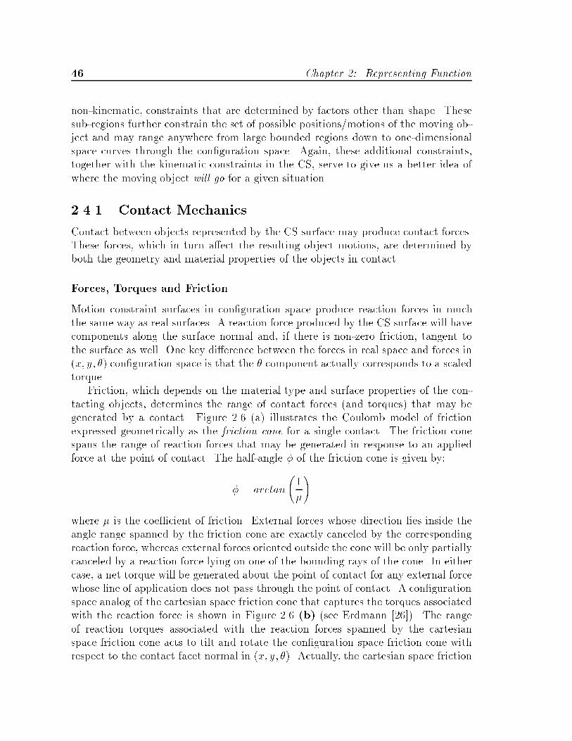
�� Chapter �� Representing Function
non�kinematic� constraints that are determined by factors other than shape� Thesesub�regions further constrain the set of possible positions�motions of the moving ob�ject and may range anywhere from large bounded regions down to one�dimensionalspace curves through the con�guration space� Again� these additional constraints�together with the kinematic constraints in the CS� serve to give us a better idea ofwhere the moving object will go for a given situation�
����� Contact Mechanics
Contact between objects represented by the CS surface may produce contact forces�These forces� which in turn a�ect the resulting object motions� are determined byboth the geometry and material properties of the objects in contact�
Forces� Torques and Friction
Motion constraint surfaces in con�guration space produce reaction forces in muchthe same way as real surfaces� A reaction force produced by the CS surface will havecomponents along the surface normal and� if there is non�zero friction� tangent tothe surface as well� One key di�erence between the forces in real space and forces in�x� y� �� con�guration space is that the � component actually corresponds to a scaledtorque�
Friction� which depends on the material type and surface properties of the con�tacting objects� determines the range of contact forces �and torques� that may begenerated by a contact� Figure ��� �a� illustrates the Coulomb model of frictionexpressed geometrically as the friction cone for a single contact� The friction conespans the range of reaction forces that may be generated in response to an appliedforce at the point of contact� The half�angle � of the friction cone is given by�
� " arctan
��
�
�
where � is the coe�cient of friction� External forces whose direction lies inside theangle range spanned by the friction cone are exactly canceled by the correspondingreaction force� whereas external forces oriented outside the cone will be only partiallycanceled by a reaction force lying on one of the bounding rays of the cone� In eithercase� a net torque will be generated about the point of contact for any external forcewhose line of application does not pass through the point of contact� A con�gurationspace analog of the cartesian space friction cone that captures the torques associatedwith the reaction force is shown in Figure ��� b� �see Erdmann ������ The rangeof reaction torques associated with the reaction forces spanned by the cartesianspace friction cone acts to tilt and rotate the con�guration space friction cone withrespect to the contact facet normal in �x� y� ��� Actually� the cartesian space friction

��� Non�Kinematic Constraints ��
X
Y
θ
X
Y
ncs
Fext
Fext
Figure ���� Coulomb friction represented as a friction cone� and the corresponding�x� y� �� con�guration space friction cone for a single contact facet�
cone may be viewed as a projection of the con�guration space friction cone into the�x� y� plane� The geometric interpretation of the con�guration space friction coneas the range of possible reaction forces and torques due to an applied force remainsunchanged�
Figure ��� illustrates the cartesian and con�guration space friction cones for asingle �type B� contact represented by a CS facet� Friction cones for contacts withedges or vertices on the CS corresponding to multiple object feature contacts arederived by computing the set sum� or Minkowski� sum� for the friction cones ofeach of the individual CS facets involved at the point of contact� The equations andmethods used to construct the con�guration space friction cones for each of the abovecontact cases are discussed in detail in Section ������� The important point to keepin mind here is the interpretation of the friction cone as a geometric representationof the set of possible reaction forces at a point on the surface of the CS�
Elastic and Inelastic Collisions
Collisions between moving objects are another form of interaction that produce re�action forces which in turn determine the resulting motion� In the simplest caseinvolving direct collisions between two objects represented as point masses� the col�
�The set sum is de�ned as� A�B fa� bja � A� b � Bg�

�� Chapter �� Representing Function
lision event may be divided into two stages� deformation and restitution��
The ratio of the restitution impulse over the deformation impulse �Poisson�s hy�pothesis� is the coe�cient of restitution�
e "
RRdtRPdt
whereRPdt is the total impulse over time during deformation�
RRdt is the total
impulse over time during restitution� and e has a value somewhere between and�� If e " � then the collision is perfectly elastic and energy as well as momentumare conserved during the collision� The coe�cient of restitution depends to a largeextent on the materials of the two objects� but may also depend on the velocitiesinvolved� as well as the shapes and sizes of the colliding objects� For the simple casedescribed above� we may take e to be a constant and use it to compute the normalvelocities of the colliding objects immediately after collision using�
e "v�B � v�AvA � vB
� �����
We should note that in general the nature of collisions can be considerably morecomplex than for the case described above �see Wang � ���� Nevertheless� we mayuse equation ��� as a rough approximation to the actual behavior of colliding objectsfor the purposes of bounding the range of possible motions involving collisions�
����� Forward Projections
As noted earlier� we are interested in determining where the moving object will go�or at least in further constraining where it might go� under a given set of conditions�What we have developed up to this point is the complete set of kinematic constraintsgiven by the CS� as well as models of interaction mechanics covering frictional slidingand inelastic collisions� What remains is to combine these with the appropriate initialconditions to construct the set of possible motions� In particular� from a speci�edset of initial conditions we will construct the motion or set of motions de�ned by theforward projection�
S� " FA�S�� �����
where S� is a point� set of points� or a region in con�guration space �state space��A is a �possibly varying� force applied to the moving object� and S� is the point�set of points� or region in con�guration space traversed by the reference point of themoving object�� An important point to keep in mind is that the forward projection
�By direct we mean that the velocities are collinear� In examples where the collision is obliquewe refer to the components of the two velocities that are collinear�
�The notation for A is derived from the term Action from the �eld of robot motion planningfrom which the de�nition of the forward projection is taken see Erdmann ������

��� Non�Kinematic Constraints ��
does not necessarily describe the exact motion of the moving object� In fact� onlywhen we have a known starting point S�� a known force A� and detailed mechanicsmodels for the interactions with the surface of the CS� will we be able to generate anexact trajectory through con�guration space for the object�s motion� In general� S�will be a bounded region in con�guration space� A will either be an exact or boundedfunction� and the models for the mechanics of interaction will be approximate� As aresult� S� will itself be a region in con�guration space which will contain� as a subset�the exact motion of the object� In those cases where we may have a number of initialpositions� or a set of discrete approximations to a region containing possible initialconditions� we may compute the overall forward projection as the union of individualforward projections� or�
FA
��i
Si
�"�i
FA �Si� �����
where i is the index to a particular subset of initial conditions� This will be par�ticularly useful later on when we will implement forward projections by means ofnumerical integration or geometrical construction�
The above description of a forward projection seems strikingly similar to thede�nition of a simulation� In fact� we may view the forward projection as a superset ofsimulations� Again� whereas a simulation describes where a system will go for a givenset of parameters� the forward projection bounds where a system can and cannot go�and is thus considered as an extension of the motion constraint set originating withthe CS� The one piece of information not included in the forward projection that isavailable in a simulation is the time history of a motion since we do not considervelocities in our state space�
We will now brie�y consider two broad classes of forward projection� one depend�ing on a relatively detailed model of local interaction� and the other relying on lessexact but more general global energy constraints� In the discussion that follows� wewill assume that the values of the parameters mentioned are known exactly unlessotherwise speci�ed� Although the construction of forward projections that incorpo�rate an explicit representation of parametric uncertainty is an important aspect ofrobust motion analysis� we will not consider such representations here due to theadditional level of complexity that doing so would introduce� Where possible� weshall adopt conservative approximations in an attempt to overcome the limitationsof not considering uncertainty explicitly� In the next chapter we will discuss a num�ber of tools and representations that may be used to examine some of the e�ects ofuncertainty� An excellent treatment of bounded parametric uncertainty applied tomotion analysis is given by Brost �����
� Chapter �� Representing Function
Numerical Simulation
Given a discrete initial position� or set of positions� along with a relatively detailedmodel of the mechanics of interaction between objects� the most direct means fordetermining where an object will go is simulation via numerical integration� Forexample� the motion of a compliantly held rigid part during an assembly operationmay be computed using a quasi�static model of dynamics where forces due to springdisplacements and Coulomb friction dominate those due to velocities and accelera�tions �see Whitney ������ Brie�y� a motion path may be integrated as follows� Ateach point in the integration� the force equilibrium at a contact point is computed�For a quasi�static model� the reaction force at the contact point is assumed to lie onthe edge of the friction cone such that the net force is approximately zero� Becausethe reaction force is at one extreme of the range of forces generated in response toan applied force� the moving object is in a state of impending motion in the direc�tion of the applied force projected into the plane tangent to the CS surface at thepoint of contact� A small incremental displacement is made along the surface in thisdirection� and the integration continues from the new position�
Where available� more complete dynamic models including damping and inertiale�ects may be included to integrate more detailed and accurate trajectories� In thosecases where initial position or other parameters are not known precisely� an approxi�mation to the forward projection may be generated by numerically integrating pathscorresponding to extremes of parameter values and bundling these paths together toform the union��
Energy Bounds for Conservative Systems
Often it will be the case that generating a detailed simulation of object motion willbe impractical or even impossible given the amount of information available aboutthe system and the characteristics of the interactions� In such cases� we may rely onsimpler� more conservative� approximations of object motions to provide an upperbound on the range of possible motions contained by the forward projection� Onesuch bound due to Brost ���� limits the possible motions of an object dropped fromrest in a gravity �eld using conservation of energy arguments� Speci�cally� Brostnoted that an object� represented by a point in an �x� y� �� con�guration space�could not reach any other point in con�guration space that had a higher relativepotential energy� no matter what �conservative� interactions took place� This boundmay be expressed geometrically as a plane through the �x� y� �� dropping point and
�Another approach due to Brost ���� is to directly integrate motion ranges at discrete points onthe surface of the CS and connect these to form boundaries of reachable regions� These boundedregions are then �lifted� from the surface of the CS into the free con�guration space to form bounded�volumes�� In Brost�s application these regions correspond to backprojections from goal regionsalthough the same mechanism may be applied to forward projections as well� See Brost �����

��� Non�Kinematic Constraints ��
perpendicular to the gravity vector which partitions the con�guration space into twohalf spaces representing reachable and unreachable con�gurations� The intersectionof the half space of reachable con�gurations and the free space bounded by the CSpresents a simple means of constructing a very conservative forward projection� In aparticularly elegant metaphor for interpreting the meaning of this forward projection�Brost likens the resulting intersections to �puddles� of water on the surface of theCS��
Recalling our earlier discussion on impacts and coe�cients of restitution� wemay interpret the plane bounding the maximum potential energy as the forwardprojection assuming perfectly elastic collisions with e " �� Since most materialshave some internal damping� we would like to examine forward projections for caseswhere e � �� i�e� where collisions are assumed to be inelastic� Let us assume that thestationary object �B� remains stationary throughout an impact� then vB " v�B " and�
v�A " �evA ����
where the minus sign indicates that the post�impact velocity of the moving object�A� is in the opposite direction to the pre�impact velocity�
Let us consider a simple example with the purpose of obtaining an approximatebound to the forward projection for a dropped object based on a value of e � ��
In Figure �� we have a particle being dropped from rest in a gravity �eld onto a�frictionless� �at surface patch tilted by an amount �� relative to the horizontal� Asecond surface patch is positioned horizontally at the same height as the �rst suchthat the particle�s parabolic trajectory after the �rst impact intersects the secondpatch� and is oriented by an amount �� such that the particle�s motion after thesecond impact is vertical� as shown in Figure �� � This particular con�guration of twoconsecutive impacts was chosen to allow us to explore the range of �x� y� excursions ofa particle with the minimumnumber of collisions �two� necessary to raise the particleback to its maximum height with zero horizontal velocity �i�e� maximum potentialenergy�� Since the position and orientation of the second patch is dependent on theorientation of the �rst patch� we may explore the range of particle motions by varyingonly one parameter ��� The lower half of Figure �� plots the locus of points� forvarious values of �� from � �
� � of �i� the maximum height hmax� reached by theparticle after impacting the �rst angled surface� and �ii� the maximum height hmax�
reached after the second impact�
�Actually the puddle metaphor is particularly useful for Brost�s application of constructing abackprojection from a goal state by slowly ��lling� the puddle from a goal state until it eitherreaches a constraint or over�ows into another region on the CS surface� The volume enclosed bythe puddle then represents the set of x� y� �� con�gurations from which an object may be droppedand still be guaranteed to reach the desired goal�
Derivations for the models used in this and the following examples are presented in Ap�pendix A���

�� Chapter �� Representing Function
The shaded region in the lower half of Figure �� represents a conservative boundon the �x� y� positions that the particle may reach or pass through for any pair ofcollisions� This region corresponds to a simple conservative model of the forwardprojection for the dropped particle� Since each semi�elastic collision involves a lossof energy� we postulate that this region contains all of the positions reachable by adropped particle for any number of collisions� Figure ��� shows a number of doublebounce maximum height curves for various values of e� We notice that� as expected�the lower the value of e� the smaller the forward projection becomes� Again� we mayconservatively approximate the boundaries of the forward projections for a droppedparticle that may undergo an arbitrary number of collisions with randomly orientedsurfaces by straight lines as shown in Figure ���� By symmetry about the verticalaxis� the forward projection for a dropped particle with a maximum coe�cient ofrestitution e becomes a cone in �x� y�� as shown in the bottom of Figure ����
We have so far neglected the role of friction and rotational motions in the for�ward projection of a dropped object� modeled here as a particle� We expect that theaddition of friction into the above models will serve to further tighten the boundson the forward projection� Also� since energy is present in rotational as well astranslational motion� we expect similar bounds to extend into the � dimension ofcon�guration space where a point represents the position and orientation of a rigidobject�� As noted earlier� the nature of impacts for rigid objects in the presenceof friction can be considerably more complex than for a particle �see Wang � ����Nevertheless� approximate models for such interactions do exist� and the above ex�amples serve to illustrate the nature of conservative models for forward projectionsof objects undergoing motions that are potentially far more complex�
Energy Bounds for Non�Conservative Systems
One more forward projection model that we will brie�y consider applies to the casewhere an object interacts with a surface undergoing a forced vibration� We mentionthis case here because it is representative of a number of real world examples� andbecause bounds on the forward projection are particularly useful in describing thebehavior of such systems since they are known to be chaotic in general���
We once again begin with a simple model consisting of a particle that is eitherdropped or placed onto a surface that is undergoing a forced oscillation of y�t� "
�One important exception noted by Brost ���� has to do with rolling motions of objects� If anobject is allowed to roll it is theoretically possible that the forward projection could extend toin�nity for interactions with a �at surface� Since we are concerned with objects represented aspolygons we do not consider this exception since any rolling motion of a polygonal object willinvolve impacts between the vertices of the moving object and the surface on which rolling takesplace� These impacts will remove energy from the moving object and eventually bring it to rest�
��For a classic example see �The Dynamics of a Bouncing Ball� Section ��� in Guckenheimeret� al� �����
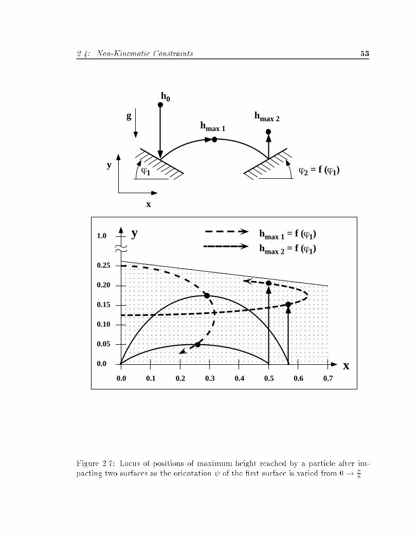
��� Non�Kinematic Constraints ��
0.25
0.20
0.15
0.10
0.05
0.0
0.1 0.2 0.3 0.4 0.5 0.6 0.70.0
1.0 hmax 1 = f (ϕ1)
hmax 2 = f (ϕ1)
y
x
h0
hmax 1
hmax 2
ϕ1 ϕ2 = f (ϕ1)
g
y
x
Figure �� � Locus of positions of maximum height reached by a particle after im�pacting two surfaces as the orientation � of the �rst surface is varied from � �
� �

�� Chapter �� Representing Function
h0 = 1.0g
y
x
ε < 1.0
0.8
0.6
0.4
0.2
0.0
0.25 0.5 0.75 1.0 1.25 1.5 1.750.0
1.0
x
ε = 1.0
ε = 0.9
ε = 0.8
ε = 0.7
ε = 0.5ε = 0.3
hmax 2 for various εy
Forward Projection Cone
Figure ���� Locus of double bounce maximum height positions for selected values ofe�
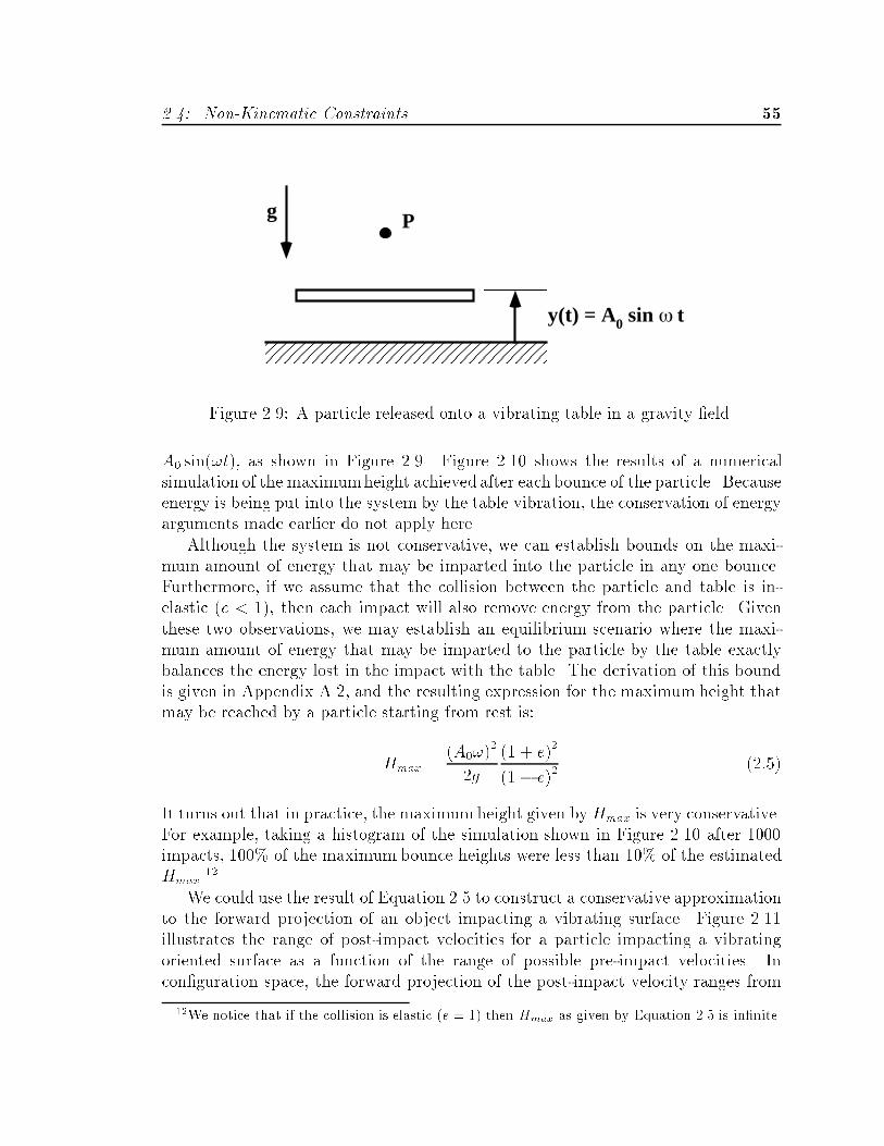
��� Non�Kinematic Constraints ��
y(t) = A0 sin ω t
Pg
Figure ���� A particle released onto a vibrating table in a gravity �eld�
A sin��t�� as shown in Figure ���� Figure ��� shows the results of a numericalsimulation of the maximumheight achieved after each bounce of the particle� Becauseenergy is being put into the system by the table vibration� the conservation of energyarguments made earlier do not apply here�
Although the system is not conservative� we can establish bounds on the maxi�mum amount of energy that may be imparted into the particle in any one bounce�Furthermore� if we assume that the collision between the particle and table is in�elastic �e � ��� then each impact will also remove energy from the particle� Giventhese two observations� we may establish an equilibrium scenario where the maxi�mum amount of energy that may be imparted to the particle by the table exactlybalances the energy lost in the impact with the table� The derivation of this boundis given in Appendix A��� and the resulting expression for the maximum height thatmay be reached by a particle starting from rest is�
Hmax "�A��
�
�g
�� � e��
��� e�������
It turns out that in practice� the maximumheight given byHmax is very conservative�For example� taking a histogram of the simulation shown in Figure ��� after �impacts� �$ of the maximum bounce heights were less than �$ of the estimatedHmax���
We could use the result of Equation ��� to construct a conservative approximationto the forward projection of an object impacting a vibrating surface� Figure ����illustrates the range of post�impact velocities for a particle impacting a vibratingoriented surface as a function of the range of possible pre�impact velocities� Incon�guration space� the forward projection of the post�impact velocity ranges from
��We notice that if the collision is elastic e �� then Hmax as given by Equation ��� is in�nite�
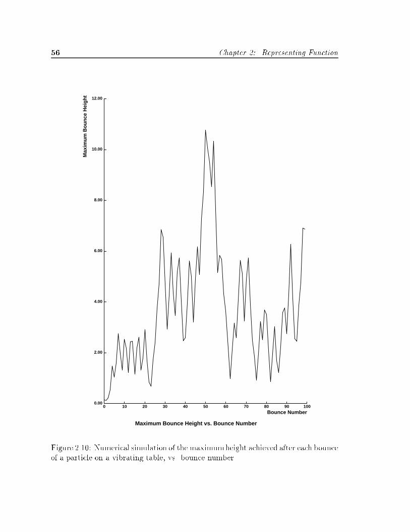
�� Chapter �� Representing Function
0.00
2.00
4.00
6.00
8.00
10.00
12.00
Max
imu
m B
ou
nce
Hei
gh
t
0 10 20 30 40 50 60 70 80 90 100Bounce Number
Maximum Bounce Height vs. Bounce Number
Figure ���� Numerical simulation of the maximumheight achieved after each bounceof a particle on a vibrating table� vs� bounce number�
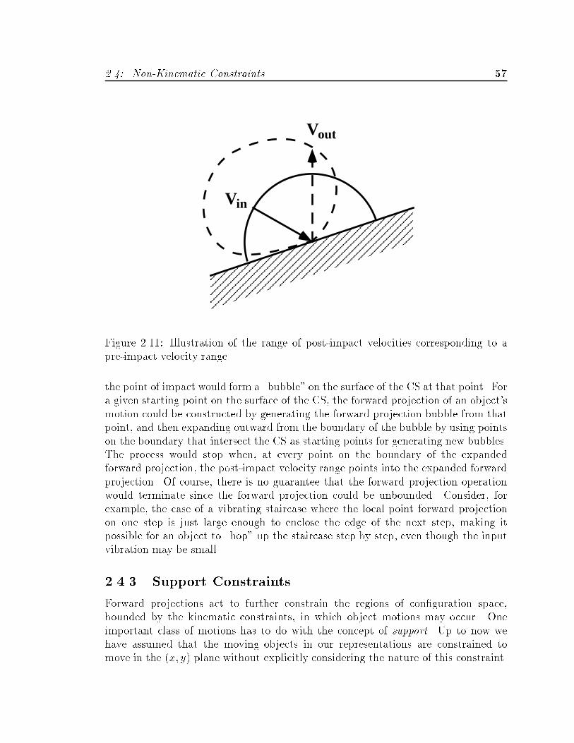
��� Non�Kinematic Constraints ��
Vin
Vout
Figure ����� Illustration of the range of post�impact velocities corresponding to apre�impact velocity range�
the point of impact would form a �bubble� on the surface of the CS at that point� Fora given starting point on the surface of the CS� the forward projection of an object�smotion could be constructed by generating the forward projection bubble from thatpoint� and then expanding outward from the boundary of the bubble by using pointson the boundary that intersect the CS as starting points for generating new bubbles�The process would stop when� at every point on the boundary of the expandedforward projection� the post�impact velocity range points into the expanded forwardprojection� Of course� there is no guarantee that the forward projection operationwould terminate since the forward projection could be unbounded� Consider� forexample� the case of a vibrating staircase where the local point forward projectionon one step is just large enough to enclose the edge of the next step� making itpossible for an object to �hop� up the staircase step by step� even though the inputvibration may be small�
����� Support Constraints
Forward projections act to further constrain the regions of con�guration space�bounded by the kinematic constraints� in which object motions may occur� Oneimportant class of motions has to do with the concept of support� Up to now wehave assumed that the moving objects in our representations are constrained tomove in the �x� y� plane without explicitly considering the nature of this constraint�
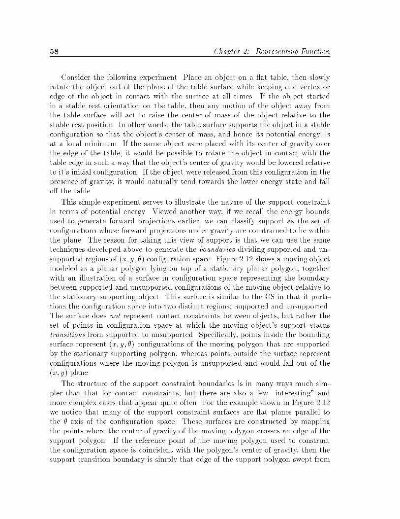
�� Chapter �� Representing Function
Consider the following experiment� Place an object on a �at table� then slowlyrotate the object out of the plane of the table surface while keeping one vertex oredge of the object in contact with the surface at all times� If the object startedin a stable rest orientation on the table� then any motion of the object away fromthe table surface will act to raise the center of mass of the object relative to thestable rest position� In other words� the table surface supports the object in a stablecon�guration so that the object�s center of mass� and hence its potential energy� isat a local minimum� If the same object were placed with its center of gravity overthe edge of the table� it would be possible to rotate the object in contact with thetable edge in such a way that the object�s center of gravity would be lowered relativeto it�s initial con�guration� If the object were released from this con�guration in thepresence of gravity� it would naturally tend towards the lower energy state and fallo� the table�
This simple experiment serves to illustrate the nature of the support constraintin terms of potential energy� Viewed another way� if we recall the energy boundsused to generate forward projections earlier� we can classify support as the set ofcon�gurations whose forward projections under gravity are constrained to lie withinthe plane� The reason for taking this view of support is that we can use the sametechniques developed above to generate the boundaries dividing supported and un�supported regions of �x� y� �� con�guration space� Figure ���� shows a moving objectmodeled as a planar polygon lying on top of a stationary planar polygon� togetherwith an illustration of a surface in con�guration space representing the boundarybetween supported and unsupported con�gurations of the moving object relative tothe stationary supporting object� This surface is similar to the CS in that it parti�tions the con�guration space into two distinct regions� supported and unsupported�The surface does not represent contact constraints between objects� but rather theset of points in con�guration space at which the moving object�s support statustransitions from supported to unsupported� Speci�cally� points inside the boundingsurface represent �x� y� �� con�gurations of the moving polygon that are supportedby the stationary supporting polygon� whereas points outside the surface representcon�gurations where the moving polygon is unsupported and would fall out of the�x� y� plane�
The structure of the support constraint boundaries is in many ways much sim�pler than that for contact constraints� but there are also a few �interesting� andmore complex cases that appear quite often� For the example shown in Figure ����we notice that many of the support constraint surfaces are �at planes parallel tothe � axis of the con�guration space� These surfaces are constructed by mappingthe points where the center of gravity of the moving polygon crosses an edge of thesupport polygon� If the reference point of the moving polygon used to constructthe con�guration space is coincident with the polygon�s center of gravity� then thesupport transition boundary is simply that edge of the support polygon swept from
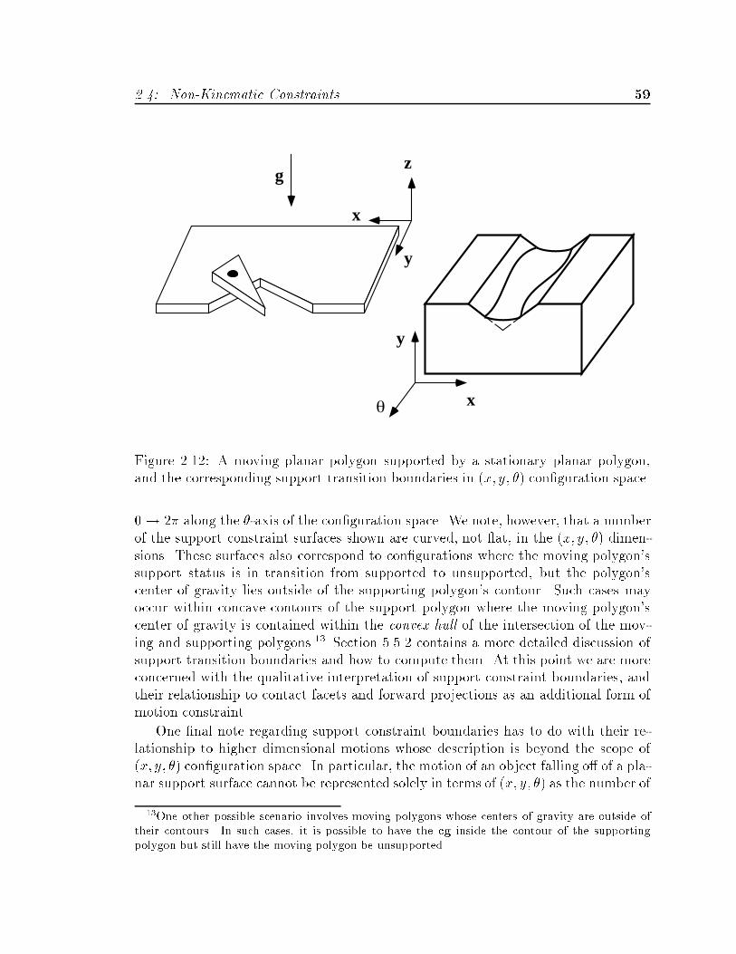
��� Non�Kinematic Constraints ��
x
y
zg
x
y
θ
Figure ����� A moving planar polygon supported by a stationary planar polygon�and the corresponding support transition boundaries in �x� y� �� con�guration space�
� � along the ��axis of the con�guration space� We note� however� that a numberof the support constraint surfaces shown are curved� not �at� in the �x� y� �� dimen�sions� These surfaces also correspond to con�gurations where the moving polygon�ssupport status is in transition from supported to unsupported� but the polygon�scenter of gravity lies outside of the supporting polygon�s contour� Such cases mayoccur within concave contours of the support polygon where the moving polygon�scenter of gravity is contained within the convex hull of the intersection of the mov�ing and supporting polygons��� Section ����� contains a more detailed discussion ofsupport transition boundaries and how to compute them� At this point we are moreconcerned with the qualitative interpretation of support constraint boundaries� andtheir relationship to contact facets and forward projections as an additional form ofmotion constraint�
One �nal note regarding support constraint boundaries has to do with their re�lationship to higher dimensional motions whose description is beyond the scope of�x� y� �� con�guration space� In particular� the motion of an object falling o� of a pla�nar support surface cannot be represented solely in terms of �x� y� �� as the number of
��One other possible scenario involves moving polygons whose centers of gravity are outside oftheir contours� In such cases it is possible to have the cg inside the contour of the supportingpolygon but still have the moving polygon be unsupported�

� Chapter �� Representing Function
degrees of freedom for such a motion� and hence the number of position parametersrequired to characterize it� are greater than three� The support constraint bound�aries just described represent those con�gurations where a planar motion representedas a trajectory in �x� y� �� would transition to a trajectory in a higher dimensionalcon�guration space of which �x� y� �� is a subset� The support constraint boundaries�then� represent a lower dimensional mapping of the transitions to higher dimensionalmotions� This transition model constitutes a tradeo� where we sacri�ce detailedknowledge of these higher dimensional motions in return for a simpler and moremanageable representation� In the next section we will examine further the use ofsuch simpli�cations that allow us to reduce the dimensionality and complexity ofmotion constraints represented in con�guration space� as well as explore ways of rep�resenting the di�erent forms of motion constraints discussed above within the sameglobal framework�
��� Mapping Constraints into Motion Space
The CS� forward projections� and support constraints all partition the con�gurationspace into regions that are either reachable or unreachable with respect to motionsof the moving object� Our purpose in generating these constraints is to combinethem in such a way as to predict the behavior� expressed as motions� of the systemunder study� In this section we will brie�y discuss some of the ways of combining thegeometric representations of motion constraint developed above within con�gurationspace so as to make such behavior explicit� The important point to keep in mind aswe manipulate the various di�erent forms of constraint representations is that theyare all expressed in terms of the motion of the moving object as captured by thecon�guration space� The factors that determine these constraints� shape� mechanicsand dynamics� are all represented implicitly in the constraints � it is the constraintson the motions themselves that are explicit�
Contact Constraints � The CS
We have already discussed the representation of contact constraints in con�gurationspace� By taking the union of contact facets for all feature pairs for a moving and sta�tionary object� we generate a representation of the entire set of kinematically distinctcontact interactions for those objects that also serves to partition the con�gurationspace into regions of reachable and unreachable positions of the moving object�
Forward Projections
The two broad classes of forward projections discussed in Section ����� i�e� exactand energy bounded� may be represented in con�guration space as one�dimensional

��� Mapping Constraints into Motion Space ��
Figure ����� A forward projection generated from a numerically integrated motionpath across the surface of a CS�
space curves and three�dimensional bounded regions� respectively� Figure ���� il�lustrates an exact trajectory for a moving object� starting from a speci�ed initialposition� represented as a space curve on the surface of the CS of Figure ��� Theforward projection consists of the set of points along the curve��� In the case ofenergy bounded motion dynamics� a �at plane �for e " �� perpendicular to the di�rection of gravity would intersect the surface of the CS� The forward projection wouldthen consist of the set of points corresponding to the volume of con�guration spacebounded below by the surface of the CS and above by the bounded energy plane�
Intersection of Contact and Support Constraints
A further simpli�cation for the support constraint regions introduced in Section �����both in terms of computation and representation� is to directly compute the intersec�
��Although rarely represented in terms of boundaries we may consider a trajectory generatedfrom exact integration of motion mechanics to be a tubular region in con�guration space boundedby motion constraints that have been collapsed onto a one�dimensional space curve� This view issemantically consistent with the much looser bounds imposed by the constraint surfaces generatedfor an energy bounded forward projection�

�� Chapter �� Representing Function
tion of the support constraint boundaries with the surface of the CS in con�gurationspace� The result is a partitioning of the surface of the CS into con�gurations wherethe moving object is� �i� in contact with the outer contour of a stationary objectin the same plane� and �ii� either supported or unsupported by a second stationaryobject underneath the plane of motion� This simpli�cation allows us to represent thesubset of support transitions that occur while an object is in contact with anotherobject in the same plane� without obscuring the display of the CS by trying to repre�sent another constraint surface in con�guration space� Figure ��� illustrates such apartitioning of the CS surface� where the darkened regions represent contact con�gu�rations that are unsupported� Since most of the motions we shall be concerned withare constrained motions where the moving object is in contact with the stationaryobject� this simpli�ed representation of support constraints preserves most of theuseful information present in the general support constraint boundary surface�
Superposition of Con guration Space Slices
As we mentioned in Section ���� we will deal primarily with interactions between ob�jects constrained to have three or fewer degrees of freedom� It is important to notethat this constraint does not require that the objects we consider must themselvesbe planar� Indeed� with a �not insigni�cant� amount of additional work and compu�tation� it is possible to represent interactions between three dimensional polyhedra�Another approximate but more convenient approach is to model three dimensionalobjects as a series of polygons corresponding to slices of the objects at di�erentheights� The � � �D CS for each of these slices may then be generated using thetools and representations described earlier in this chapter and then superimposedwithin the same �x� y� �� con�guration space� The resulting composite CS structure�although somewhat more complex and with a much larger number of contact facets�many of which would be occluded by other facets�� could be used for analysis inmuch the same manner as the CS for a single set of polygon interactions���
Other Constraint Mappings
There are a number of other mappings of constraints to con�guration space that�depending on the application� can be useful in representing function in terms ofmotion� The following three constraint mappings are due to Brost ���� and were
��One caveat to this approach has to do with the fact that interactions with the CS surface thatcorrespond to contacts among slices at di�erent heights would impose out of plane torques to theobject that would be outside the scope of the x� y� �� representation� Special care would haveto be taken to ensure that the distribution of forces among the slices in contact was consistent�Techniques analogous to the support transition boundaries of Section ����� might also be useful inrepresenting the e�ects of these torques�

��� Mapping Constraints into Motion Space ��
X
Y
Figure ���� Support transition boundaries intersected with the surface of the CS�
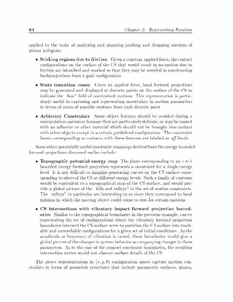
�� Chapter �� Representing Function
applied to the tasks of analyzing and planning pushing and dropping motions ofplanar polygons�
� Sticking regions due to friction� Given a constant applied force� the contactcon�gurations on the surface of the CS that would result in no motion due tofriction are identi�ed and marked so that they may be avoided in constructingbackprojections from a goal con�guration�
� State transition cones� Given an applied force� local forward projectionsmay be generated and displayed at discrete points on the surface of the CS toindicate the ��ow� �eld of constrained motions� This representation is partic�ularly useful in capturing and representing uncertainty in motion parametersin terms of cones of possible motions from each discrete point�
� Arbitrary Constraints� Some object features should be avoided during amanipulation operation because they are particularly delicate� or may be coatedwith an adhesive or other material which should not be brought into contactwith other objects except in a certain prede�ned con�guration� The constraintfacets corresponding to contacts with these features are labeled as o� limits�
Some other potentially useful constraint mappings derived from the energy boundedforward projections discussed earlier include�
� Topographic potential energy map� The plane corresponding to an e " �bounded energy forward projection represents a constraint for a single energylevel� It is not di�cult to imagine generating curves on the CS surface corre�sponding to slices of the CS at di�erent energy levels� Such a family of contourswould be equivalent to a topographical map of the CS surface� and would pro�vide a global picture of the �hills and valleys� in the set of motion constraints�The �valleys� in particular are interesting to us since they correspond to localminima in which the moving object could come to rest for certain motions�
� CS intersections with vibratory impact forward projection bound�aries� Similar to the topographical boundaries in the previous example� curvesrepresenting the set of con�gurations where the vibratory forward projectionboundaries intersect the CS surface serve to partition the CS surface into reach�able and unreachable con�gurations for a given set of initial conditions� As theamplitude or frequency of vibration is varied� these boundaries would give aglobal picture of the changes in system behavior accompanying changes in theseparameters� As in the case of the support constraint boundaries� the resultingintersection curves would not obscure surface details of the CS�
The above representations in �x� y� �� con�guration space capture motion con�straints in terms of geometric structures that include parametric surfaces� planes�
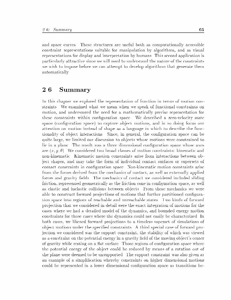
�� � Summary ��
and space curves� These structures are useful both as computationally accessibleconstraint representations suitable for manipulation by algorithms� and as visualrepresentations for display and interpretation by humans� This second application isparticularly attractive since we will need to understand the nature of the constraintswe wish to impose before we can attempt to develop algorithms that generate themautomatically�
��� Summary
In this chapter we explored the representation of function in terms of motion con�straints� We examined what we mean when we speak of functional constraints onmotion� and underscored the need for a mathematically precise representation forthese constraints within con�guration space� We described a zero�velocity statespace �con�guration space� to capture object motions� and in so doing focus ourattention on motion instead of shape as a language in which to describe the func�tionality of object interactions� Since� in general� the con�guration space can bequite large� we limited our discussion to objects whose motions were constrained tolie in a plane� The result was a three dimensional con�guration space whose axesare �x� y� ��� We considered two broad classes of motion constraints� kinematic andnon�kinematic� Kinematic motion constraints arise from interactions between ob�ject shapes� and may take the form of individual contact surfaces or supersets ofcontact constraints in con�guration space� Non�kinematic motion constraints arisefrom the forces derived from the mechanics of contact� as well as externally appliedforces and gravity �elds� The mechanics of contact we considered included slidingfriction� represented geometrically as the friction cone in con�guration space� as wellas elastic and inelastic collisions between objects� From these mechanics we wereable to construct forward projections of motions that further partitioned con�gura�tion space into regions of reachable and unreachable states� Two kinds of forwardprojection that we considered in detail were the exact integration of motions for thecases where we had a detailed model of the dynamics� and bounded energy motionconstraints for those cases where the dynamics could not easily be characterized� Inboth cases� we likened forward projections to a timeless superset of simulations ofobject motions under the speci�ed constraints� A third special case of forward pro�jection we considered was the support constraint� the stability of which was viewedas a constraint on the potential energy in a gravity �eld of the moving object�s centerof gravity while resting on a �at surface� Those regions of con�guration space wherethe potential energy of the object could be reduced by means of a rotation out ofthe plane were deemed to be unsupported� The support constraint was also given asan example of a simpli�cation whereby constraints on higher dimensional motionscould be represented in a lower dimensional con�guration space as transitions be�

�� Chapter �� Representing Function
tween planar and non�planar motions� Finally� after characterizing the above set ofmotion constraints� we examined various means by which those constraints could becombined within the con�guration space representation�
The purpose of this chapter was to develop the representations that will serve asthe foundation upon which we may build a set of tools that will allow us to performboth analysis and design of functionally useful shapes� To make these representationsand visualization techniques more concrete� in the next chapter we will introduce aset of four examples� peg�in�hole assembly� vibratory bowl feeders� assembly palletsand �xtures� and another vibratory feeder known as APOS� These examples havebeen chosen because they span the set of constraint representations developed here�as well as to highlight similarities among and di�erences between the various formsof functional constraints�

Visualization and Application
DomainsChapter �
In this chapter we will examine four application domains introduced in Figure ����compliant assembly� vibratory bowl feeders� assembly �xtures� and the APOS vibra�tory feeding system� We will use the motion constraint representations developed inthe previous chapter to visualize� reason about and analyze the functional charac�teristics of examples from each of these domains in terms of motion constraints�
In Section ����� we referred to the similarities between the surface of a CS facetand a �real� surface that produced reaction forces and torques in response to appliedforces� In Section ����� we referred to features on the surface of the CS using termssuch as valleys� ridges� and peaks that convey images of multiple features combiningto form what amounts to a landscape in con�guration space� The intent of this visualimagery is to convey an intuitive feel for some of the structure imbedded in the CSand how these constraints act to guide motions of a point representing the motionof a physical object�
A point in con�guration space� whose �x� y� components correspond to the posi�tion of the reference point of� and the � component to the orientation of� the movingobject can be thought of as the point of action through which external and reactionforces act to constrain the motion of the object� All interactions between shapesof both the moving and stationary objects are combined so as to be local to thispoint� If we imagine that point as a ball bouncing or sliding across the surface of theCS constraints� then we have a powerful metaphor with which to visualize how con�straints interact� For example� we have discussed energy in terms of non�kinematicconstraints� or bounds� that determine where a point� or ball� may travel in thepresence of an externally applied motive force such as weight due to gravity� Thisenergy imposes on the con�guration space a sense of up and down that immediatelyimplies a sense of where the ball will and will not go based on its interaction withthe CS surface� The curved surfaces of individual CS facets guide the motion of theball along curved trajectories imposed by the ever�changing surface normal along the
�
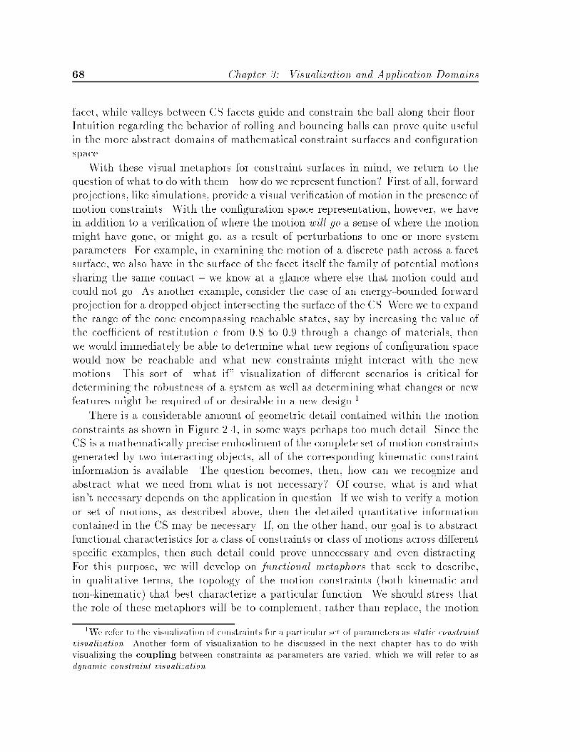
�� Chapter �� Visualization and Application Domains
facet� while valleys between CS facets guide and constrain the ball along their �oor�Intuition regarding the behavior of rolling and bouncing balls can prove quite usefulin the more abstract domains of mathematical constraint surfaces and con�gurationspace�
With these visual metaphors for constraint surfaces in mind� we return to thequestion of what to do with them � how do we represent function� First of all� forwardprojections� like simulations� provide a visual veri�cation of motion in the presence ofmotion constraints� With the con�guration space representation� however� we havein addition to a veri�cation of where the motion will go a sense of where the motionmight have gone� or might go� as a result of perturbations to one or more systemparameters� For example� in examining the motion of a discrete path across a facetsurface� we also have in the surface of the facet itself the family of potential motionssharing the same contact � we know at a glance where else that motion could andcould not go� As another example� consider the case of an energy�bounded forwardprojection for a dropped object intersecting the surface of the CS� Were we to expandthe range of the cone encompassing reachable states� say by increasing the value ofthe coe�cient of restitution e from �� to �� through a change of materials� thenwe would immediately be able to determine what new regions of con�guration spacewould now be reachable and what new constraints might interact with the newmotions� This sort of �what if� visualization of di�erent scenarios is critical fordetermining the robustness of a system as well as determining what changes or newfeatures might be required of or desirable in a new design��
There is a considerable amount of geometric detail contained within the motionconstraints as shown in Figure ��� in some ways perhaps too much detail� Since theCS is a mathematically precise embodiment of the complete set of motion constraintsgenerated by two interacting objects� all of the corresponding kinematic constraintinformation is available� The question becomes� then� how can we recognize andabstract what we need from what is not necessary� Of course� what is and whatisn�t necessary depends on the application in question� If we wish to verify a motionor set of motions� as described above� then the detailed quantitative informationcontained in the CS may be necessary� If� on the other hand� our goal is to abstractfunctional characteristics for a class of constraints or class of motions across di�erentspeci�c examples� then such detail could prove unnecessary and even distracting�For this purpose� we will develop on functional metaphors that seek to describe�in qualitative terms� the topology of the motion constraints �both kinematic andnon�kinematic� that best characterize a particular function� We should stress thatthe role of these metaphors will be to complement� rather than replace� the motion
�We refer to the visualization of constraints for a particular set of parameters as static constraint
visualization� Another form of visualization to be discussed in the next chapter has to do withvisualizing the coupling between constraints as parameters are varied which we will refer to asdynamic constraint visualization�

���� Assembly ��
constraints described earlier�
Application Domains
The assortment of representations and constraint mappings discussed in the previoussections �contact facets� forward projections and support constraints� allow us torepresent a rich set of motion constraints within the �x� y� �� con�guration space� Wewill now apply various combinations of these representations to a series of speci�cexample domains� In so doing� we hope to make the visualization concepts discussedabove more concrete� as well as explore and illustrate the properties and potentialusefulness of functional representation using motion constraints� Speci�cally� we willexamine and discuss four example domains where function is derived from motionsdominated by shape interactions� The discussion here is intended to be illustrativein nature� In the next chapter we will develop two of the examples in greater detailby implementing a computational environment supporting a set of tools to be usedfor visualization and design�
��� Assembly
Figure ��� illustrates what has become a classic instantiation of the assembly prob�lem� the task of inserting a cylindrical peg into a tight clearance hole� Accomplishingthis task is complicated by the fact that the position of the peg may not be well knownnor the assembly trajectory of the robot precisely controlled due to the presence ofuncertainties in position and control� To compensate for positional misalignments�the connection between the peg and the robot incorporates a degree of compliancethat is implemented either in hardware� such as a compliant spring device like theRemote Center of Compliance �RCC�� or by means of software control of the robotitself ���� ��� Typical failure modes of an assembly operation include jamming�where the forces between the peg and hole are balanced due to friction so that nomotion occurs� or wedging� where the compliance of the peg itself can result in signif�icant reaction forces between the peg and hole that are independent of any externalapplied forces and prevent the peg from being moved into or removed from the hole�see Whitney ������
Figure ��� shows a commonly used representation for axisymmetric parts� whereboth the peg and hole are modeled as planar polygons� The compliance can bemodeled as a generalized spring or generalized damper� For the generalized springmodel we have�
�x� x� " �C�F
where the diagonal compliance matrix �C� maps displacements� between the positionx of a reference point on the peg and the commanded position �vecx of that point
along a nominal assembly trajectory of the robot� to forces and torques F applied to
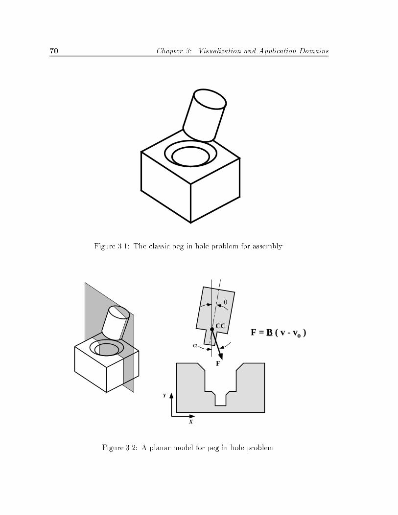
� Chapter �� Visualization and Application Domains
Figure ���� The classic peg in hole problem for assembly�
θ
CC
F
α
X
Y
F = B ( v - vo )
Figure ���� A planar model for peg in hole problem�

���� Assembly ��
Goal
"Chamfers"
Figure ���� Functional metaphor for peg in hole assembly in terms of motion con�straints�
the peg at the reference point� The elements of the compliance matrix� as well as thelocation of the reference point �the compliance center� are important parameters inaddition to part shape that must be considered in designing a successful assembly��
Compliance based on a generalized damper may be modeled in a similar fashionwith displacements replaced by di�erences in velocity� as shown in Figure ���� Weuse an approximate model of positional uncertainty where motions are integratedfrom discrete points within a bounded starting region that has been subdivided�The resulting bundle of discrete paths provides a crude model of the range of motionspossible under uncertainty� Each path may have associated with it a probability thatmay be used to determine the overall relative reliability of the assembly operationshould some of the paths in the bundle fail to reach the goal�
A metaphor for the function embodied in the assembly task in terms of motionconstraints is a funnel as shown in Figure ���� Essentially� a successful assembly ischaracterized by a class of motions starting from a set of initial starting con�gurationsthat are constrained to reach a single goal state or region due to motion constraintinteractions� These motion constraints arise from the kinematic constraints imposedby the contacts between the two part shapes and non�kinematic constraints derivedfrom friction and compliance�
Figure �� shows the con�guration representation of a planar peg in hole assembly�We can see that the physical attributes we associate with a hole are retained in theconstraints formed by the CS� Speci�cally� the goal state where the bottom of the peg
�As noted earlier active compliance may be implemented in software in which case the compli�ance matrix need not be diagonal see Schimmels and Peshkin ������

�� Chapter �� Visualization and Application Domains
is at the bottom of the hole corresponds to a region at the bottom of a correspondinghole in the CS bounded by constraint facets� If we were to take a slice of the CS inthe �x� y� plane perpendicular to the � axis at � " � the width of the CS hole wouldbe equivalent to the clearance between the peg and hole# the greater the clearance�the wider the hole� Correspondingly� if the peg were slightly larger than the hole�say for an interference �t� then the hole in the CS would disappear�
With regards to the metaphor of a motion constraint funnel� the most importantregion on the CS is the entry region immediately surrounding the hole� The facetsforming this region are the constraints that will guide assembly motions� whose initialpositions and trajectories will vary in the presence of uncertainty� toward the throatof the hole� Once the motions reach the throat of the hole the remaining portions oftheir trajectories are tightly constrained toward the goal state at the bottom of thehole �Caine ������
The idea of letting geometric constraints guide an assembly is a well known strat�egy identi�ed by a number of researchers� and formalized in terms of motion con�straints by Mason ���� A geometrical feature often employed as an aid in assemblyis the chamfer� which can be viewed as a direct physical instantiation of the motionconstraint funnel metaphor� An interesting analog to the chamfer is embodied in thecompliant motion strategy of intentionally introducing a rotational and positionalo�set by tilting the peg relative to the hole before insertion �Inoue ����� By tiltingthe peg and placing its lower corner into the hole it is possible to increase the set ofinitial starting positions from which the peg may be inserted� The result� shown incon�guration space in Figure ��� a�� is a local entry region on the CS surface that�like the set of constraints for the chamfered hole shown in b�� guides motions towardthe throat of the hole� In both cases� an entire range of trajectories is captured andguided by the funnel�like motion constraints� thus improving the overall reliability ofthe assembly operation� There is one important di�erence between chamfers and thetilting strategy� straight�line pushing motions alone are not su�cient to perform thetilting strategy since the peg must eventually be aligned with the axis of the hole toeliminate the signi�cant initial angular o�set� Hence� the tilting strategy can requirea greater degree of complexity in terms of assembly hardware� although passive de�vices have been developed which extend to this case for simple part geometries �seeDraper ����� Caine ����� Strip � ����
Generally speaking� increasing the size of the funnel�like region of the CS sur�rounding the hole is desirable in improving assembly reliability� Typically the dimen�sions of the CS hole itself� i�e� the clearance between the peg and the hole� are �xedby non�assembly design considerations such as maximum allowed slop in a bearingassembly� for example� Parameters that contribute to the motion constraints are thegeometrical features of the peg bottom and hole rim� the position of the compliance
�See for example Simunovic and Whitney �����
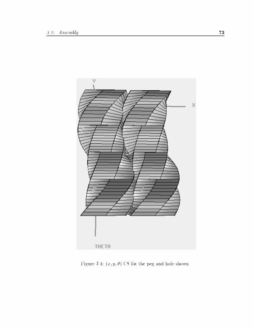
���� Assembly ��
Figure ��� �x� y� �� CS for the peg and hole shown�
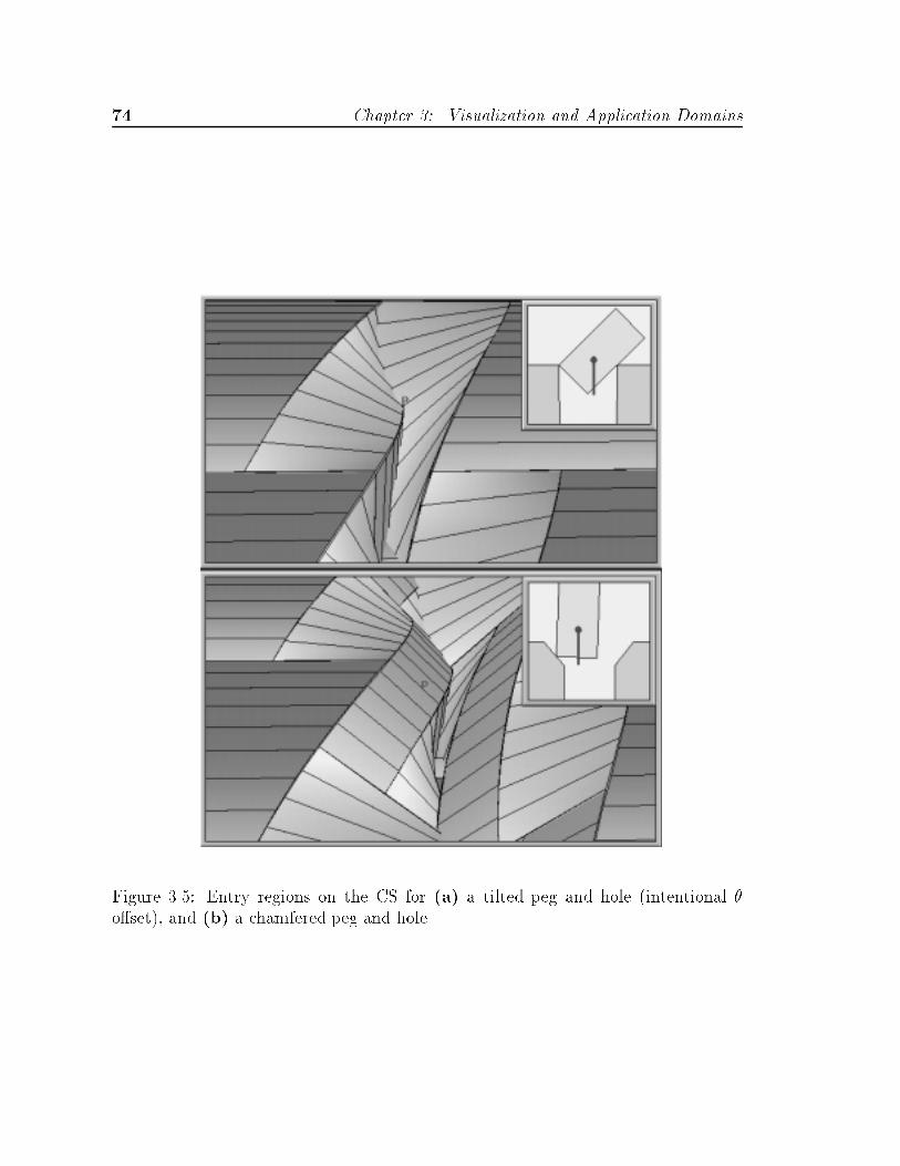
�� Chapter �� Visualization and Application Domains
Figure ���� Entry regions on the CS for a� a tilted peg and hole �intentional �o�set�� and b� a chamfered peg and hole�

���� Vibratory Bowl Feeders ��
center �reference point� on the peg� and non�kinematic parameters including the co�e�cient of friction � and compliance matrix �C�� In Section �� we will examine ingreater detail the relationships between these parameters as well as develop the toolsand strategies that will allow us to manipulate them for the purposes of designingmore reliable assemblies�
��� Vibratory Bowl Feeders
In Section ��� we gave a very brief description of a portion of a vibratory bowl feedertrack used to orient small parts� We will now complete this description and developthe appropriate representations to model feeder function� Figure ��� shows a typicalvibratory bowl feeder used to sort small parts for an automated assembly system�A large number of unoriented parts are placed in the bowl and driven up the spiraltrack on the bowl�s interior by vibratory motion� Parts reach the top of the trackin single �le in one of a �nite number of stable orientations as shown in Figure �� �As the parts reach the top of the track� they pass through a series of features builtinto the track and bowl wall designed to �i� reorient certain part con�gurations� or�ii� reject parts in an undesirable orientation by causing them to fall o� the trackand back into the bowl to be recirculated� Some typical track features are shownin Figure ���� The desired result is a series of parts in a single known orientationexiting the outlet of the feeder to be placed into a �xture or pallet by a robot orother transfer device�
One could argue that the term feeder used to refer to the device consisting ofthe bowl and track is something of a misnomer in that the bowl and track geometriesonly perform the function of feeding for a speci�c part or set of parts� Parts otherthan those for which the bowl and track were designed would not be fed properly ifplaced in the bowl� Thus� from a functional standpoint� the �feeder� is distributedbetween both the part geometries and the bowl�track geometries with which theparts interact�
The second form of part feeding operation listed above ��ii� reject parts in unde�sirable orientations� can be characterized as a �lter on part motions� In the vibratorybowl feeder� parts moving along the track in a number of di�erent initial orientationsinteract with bowl and track geometries like those shown in Figure ��� and undergodi�erent classes of motions depending on the characteristic constraints imposed bythose interactions� We identify two broad classes of motions consisting of an acceptmotion in which part is allowed to continue to remain on the track� and a series ofreject motions where the parts are forced o� of the track by removing their support�Figure ��� illustrates a motion constraint metaphor for this process where a seriesof discrete motions� corresponding to parts traveling in each of the initial stable ori�entations� are �ltered into either a single accept motion or a series of reject motions

�� Chapter �� Visualization and Application Domains
Figure ���� A vibratory bowl feeder� The bowl at the top is driven in a combinedvertical and rotary oscillatory motion by the electromagnet and springs at the bot�tom� causing small parts placed in the bowl to move in single �le up the spiral trackon the bowl�s interior� From Boothroyd et� al� � ��
Figure �� � Parts arrive at the top of the track in one of a number of stable orienta�tions� From Boothroyd et� al� � ��
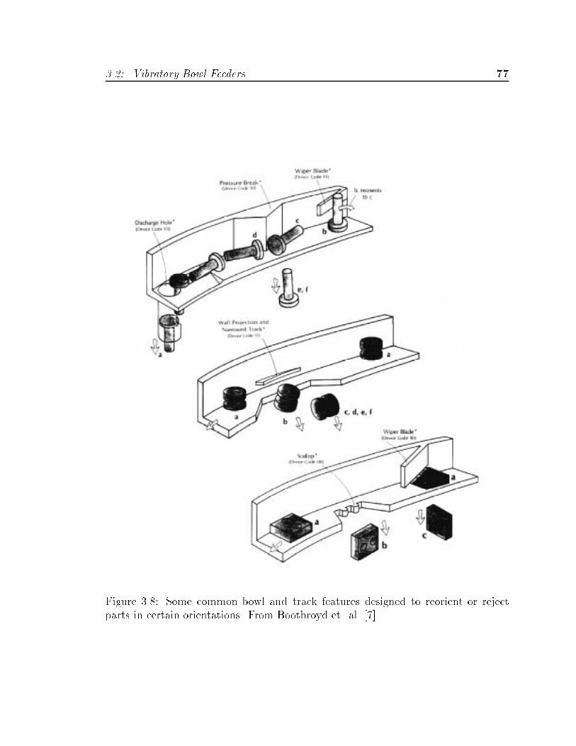
���� Vibratory Bowl Feeders ��
Figure ���� Some common bowl and track features designed to reorient or rejectparts in certain orientations� From Boothroyd et� al� � ��
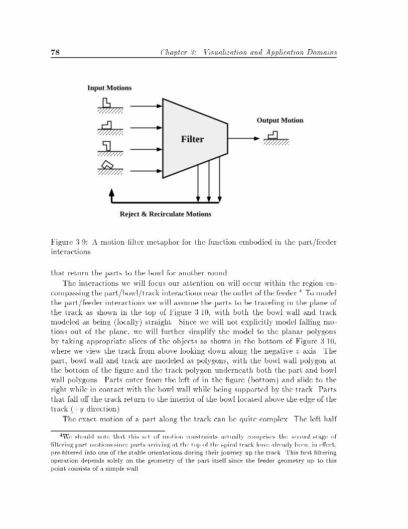
�� Chapter �� Visualization and Application Domains
Filter
Output Motion
Input Motions
Reject & Recirculate Motions
Figure ���� A motion �lter metaphor for the function embodied in the part�feederinteractions�
that return the parts to the bowl for another round�
The interactions we will focus our attention on will occur within the region en�compassing the part�bowl�track interactions near the outlet of the feeder�� To modelthe part�feeder interactions we will assume the parts to be traveling in the plane ofthe track as shown in the top of Figure ���� with both the bowl wall and trackmodeled as being �locally� straight� Since we will not explicitly model falling mo�tions out of the plane� we will further simplify the model to the planar polygonsby taking appropriate slices of the objects as shown in the bottom of Figure ����where we view the track from above looking down along the negative z axis� Thepart� bowl wall and track are modeled as polygons� with the bowl wall polygon atthe bottom of the �gure and the track polygon underneath both the part and bowlwall polygons� Parts enter from the left of in the �gure �bottom� and slide to theright while in contact with the bowl wall while being supported by the track� Partsthat fall o� the track return to the interior of the bowl located above the edge of thetrack ��y direction��
The exact motion of a part along the track can be quite complex� The left half
�We should note that this set of motion constraints actually comprises the second stage of�ltering part motions since parts arriving at the top of the spiral track have already been in e�ectpre��ltered into one of the stable orientations during their journey up the track� This �rst �lteringoperation depends solely on the geometry of the part itself since the feeder geometry up to thispoint consists of a simple wall�

���� Vibratory Bowl Feeders ��
X Y
Z
X
Y
θ+
Figure ���� A polyhedral model of a portion of the feeder track near the outlet ofthe bowl �top�� and an equivalent planar model viewed from above �bottom��

� Chapter �� Visualization and Application Domains
N
Ff
mp g
mp ao ω2
ψ
ϕ
Input Vibration:ao Sin ω t
Η
S
h
Figure ����� Force equilibrium for a part in contact with the track �left�� and atypical hopping�sliding motion for a part on the track �right�� Both illustrations arein the vertical plane containing the gravity vector g�
of Figure ���� illustrates the forces acting on a part in contact with the track in avertical plane containing the gravity vector g where mp is the mass of the part� � isthe inclination of the track relative to the horizontal� a�� is the acceleration of thebowl due to vibration� � is the angle between the vibration acceleration and the tracksurface� N is the normal and F the frictional forces between the part and the track�The right half of Figure ���� illustrates the various modes of part motion includinghopping and sliding� where the hopping height h is normal to the track� and thehopping distance H and sliding distance S are both parallel to the track� For mostreasonable values of the vibration parameters ao� � and �� the hopping height h isone to two orders of magnitude smaller than either of the sliding motions H and S��
To simplify the analysis� we will approximate the overall motion of the part on thetrack as being purely sliding� Furthermore� we will combine the part�s mass and theapplied accelerations due to vibration and gravity into one force applied to the part�scenter of gravity �i�e� CS reference point�� and will only consider the componentsparallel to the �x� y� plane of motion� Finally� since the average velocity of the part�smacroscopic motion is constant and relatively small� we will model the dynamics ofpart motion as being quasi�static�
Figure ���� shows the CS and support constraints in con�guration space for aplanar vibratory bowl feeder example �from Figure ��� a��� The CS representsthe kinematic motion constraints due to interactions between the part and bowlwall only� The highlighted regions on the surface of the CS represent those points
�Often feeder tracks are covered with a rubber coating to absorb impact energy i�e� e � � inorder to keep the part motions deterministic see Boothroyd et� al� �����

���� Vibratory Bowl Feeders ��
Figure ����� Con�guration space representation of a planar bowl feeder example�
in con�guration space where the part is in contact with the bowl wall but is notsupported by the track �see Sections ���� and ����� The paths illustrated on thesurface of the CS represent motions of parts along the track in contact with thebowl wall from each of the stable initial starting orientations �also shown�� Thethickness of each path is drawn proportional to the relative probability that a partwill enter the feeder in that initial orientation� with the thickest paths having thehighest probability and the thinnest having the least� In the example shown� wenotice that all but one of the motions paths enter one of the unsupported regionsand terminate at the boundary marking the �x� y� �� position where the part will fallo� the track and back into the bowl� The one remaining path exits the feeder to theright� corresponding to the outlet of the bowl feeder� Recalling the �lter metaphor ofFigure ���� the �nite number of discrete paths entering the feeder are �ltered into onepass motion �path number ��� and a number of reject motions �paths � �� ��� Theresult is an explicit representation of the feeding function derived from the interactionbetween the part and the feeder geometries�
We will examine the vibratory bowl feeder domain in greater detail in the nextchapter on design� For the moment we will brie�y discuss some of the major char�acteristics of feeder function as represented in con�guration space� We begin by
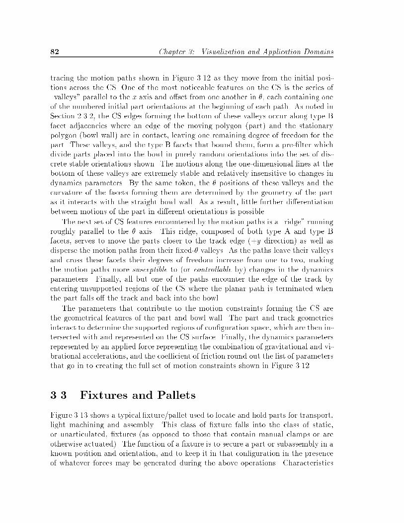
�� Chapter �� Visualization and Application Domains
tracing the motion paths shown in Figure ���� as they move from the initial posi�tions across the CS� One of the most noticeable features on the CS is the series of�valleys� parallel to the x axis and o�set from one another in �� each containing oneof the numbered initial part orientations at the beginning of each path� As noted inSection ������ the CS edges forming the bottom of these valleys occur along type Bfacet adjacencies where an edge of the moving polygon �part� and the stationarypolygon �bowl wall� are in contact� leaving one remaining degree of freedom for thepart� These valleys� and the type B facets that bound them� form a pre��lter whichdivide parts placed into the bowl in purely random orientations into the set of dis�crete stable orientations shown� The motions along the one�dimensional lines at thebottom of these valleys are extremely stable and relatively insensitive to changes indynamics parameters� By the same token� the � positions of these valleys and thecurvature of the facets forming them are determined by the geometry of the partas it interacts with the straight bowl wall� As a result� little further di�erentiationbetween motions of the part in di�erent orientations is possible�
The next set of CS features encountered by the motion paths is a �ridge� runningroughly parallel to the � axis� This ridge� composed of both type A and type Bfacets� serves to move the parts closer to the track edge ��y direction� as well asdisperse the motion paths from their �xed�� valleys� As the paths leave their valleysand cross these facets their degrees of freedom increase from one to two� makingthe motion paths more susceptible to �or controllable by� changes in the dynamicsparameters� Finally� all but one of the paths encounter the edge of the track byentering unsupported regions of the CS where the planar path is terminated whenthe part falls o� the track and back into the bowl�
The parameters that contribute to the motion constraints forming the CS arethe geometrical features of the part and bowl wall� The part and track geometriesinteract to determine the supported regions of con�guration space� which are then in�tersected with and represented on the CS surface� Finally� the dynamics parametersrepresented by an applied force representing the combination of gravitational and vi�brational accelerations� and the coe�cient of friction round out the list of parametersthat go in to creating the full set of motion constraints shown in Figure �����
��� Fixtures and Pallets
Figure ���� shows a typical �xture�pallet used to locate and hold parts for transport�light machining and assembly� This class of �xture falls into the class of static�or unarticulated� �xtures �as opposed to those that contain manual clamps or areotherwise actuated�� The function of a �xture is to secure a part or subassembly in aknown position and orientation� and to keep it in that con�guration in the presenceof whatever forces may be generated during the above operations� Characteristics

���� Fixtures and Pallets ��
Figure ����� An illustration of a typical �xture�pallet used in automated assembly�
that are desirable for a �xture include�
�� the ability to hold parts in a known con�guration that is also easily and reliablyreachable when placing the part in the �xture�
�� the ability to hold parts stably under a variety of external loads applied to thepart�
�� provides access to the parts by other parts� grippers� or tools as necessary� and
� the part or subassembly may be removed once the desired operation has beenperformed�
There are a number of other �xture characteristics not listed above whose relativeimportance depends on the application� By no means the least of these other charac�teristics is the requirement that the �xture be as inexpensive and quickly producibleas possible� Fixtures are a component of virtually every manufacturing system� bothmanual and automated� As noted in the section on vibratory bowl feeders� a consid�erable portion of the �xed capital cost for a manufacturing system consists of feedersand �xtures� Since the geometry of the �xture depends heavily on the geometry ofthe parts and the type of manufacturing operation� �xtures must typically be customdesigned for each application� Therefore� tools and techniques that would improvethe productivity and performance of �xture design would be extremely valuable�
Functionally� a �xture shares a great deal in common with an assembly� Thegoal� in terms of motions� is to place a part into the �xture in a known position and

�� Chapter �� Visualization and Application Domains
Goal
Figure ���� Functional metaphor for dropping a part into a �xture in terms ofmotion constraints�
orientation in the presence of uncertainty� Like Figure ���� the kinematic motionconstraints due to the part��xture interaction may be considered to form a funnelwhich� in the ideal case� will guide the part to the desired location from a range ofinitial positions� The main di�erence between �xtures and assembly is the nature ofthe forward projection constraining the motions of the part� Whereas we consideredan assembly to consist of a compliantly held part �peg� guided along a nominaltrajectory by a device such as a robot� we view the task of inserting a part into a�xture as one of dropping the part into place from some height in a gravity �eld� Asa result� the bounded�energy forward projection for conservative systems� as shownin Figure ���� is a more appropriate model� �
As for assembly� we will use a planar model of a part and �xture� with gravityassumed to lie in the plane of the �gure pointing down� as shown in Figure ����� Likethe assembly model� the plane in which �x� y� �� motions may take place is chosento capture the relevant geometrical features of both the part and the �xture� Foraxisymmetric objects the plane is chosen to contain the axis of symmetry� We assumethat the part is dropped with zero initial velocity above the �xture from within abounded range of initial positions and orientations� The coe�cient of friction � andcoe�cient of restitution e for the two parts are assumed to be known constants�
�We consider those cases where grasped parts are placed into the �xture using compliant motionto be an assembly and model them in the same way as described for the peg in hole example� Inthe context of motion constraints there is no distinction between a �xture and a subassembly insuch cases�

���� Fixtures and Pallets ��
c.g.
mg
X
Y
Figure ����� A planar model of a part dropped into a �xture�
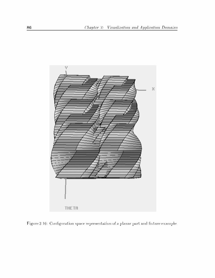
�� Chapter �� Visualization and Application Domains
Figure ����� Con�guration space representation of a planar part and �xture example�
���� Fixtures and Pallets ��
The con�guration space representation of the part��xture interaction is shownin Figure ����� We see a strong resemblance between Figure ���� and Figure ��showing the CS for the peg in hole example� The �throat� of the CS hole for a�xture is somewhat wider and shallower in comparison to that for the peg in holeassembly� but the entry region around the hole has many of the same funnel�likecharacteristics intended to guide motions toward the goal state at the bottom of thehole�
The primary di�erence between the �xture and assembly is the use of an energybounded forward projection model rather than that of a path produced by compliantmotion �see Section ������ The resulting forward projection would appear as apolyhedral cone� similar to that illustrated in the lower half of Figure ���� with itscentral axis parallel to the gravity vector in the �x� y� �� con�guration space��
The CS and forward projection representations described above address the �rstof the desirable characteristics for a �xture listed above� namely the ability to get apart into a known con�guration and keeping it there� To address the second issueof holding a part stably under a variety of loads once the part has reached the goalcon�guration� we return to our discussion of the con�guration space friction cone�We recall from Section ���� that the friction cone spans the set of reaction forcesthat will maintain equilibrium for an object� The negation of this cone� therefore�represents the set of applied forces� and torques� that may be applied to the partwithout any motion resulting� The larger the span of the friction cone� the morestably the part will be held in the presence of applied loads� Of course� the caveat isthat the same frictional e�ects that help keep the part in place are also the frictionale�ects that can make getting the part into the desired con�guration more di�cult�
The third desirable characteristic of a �xture providing access to the securedpart by other parts� grippers� or tools has to do with the kinematic constraintsbetween the �xture and these other objects� Speci�cally� we wish to determine ifthe gripper�part�tool will come into contact with the �xture during it�s operationon the part being held in the �xture�� In terms of the above representation� if thereference point of the moving object is chosen to coincide with the reference point�i�e� cg� of the part when that object was interacting with the part �grasping it� forexample�� then the CS for the object��xture interaction could be superimposed ontothe part��xture CS to produce the complete set of kinematic motion constraints onthe part� �xture and object� This superposition is the same as that discussed inSection ��� for superimposing CS constraints for interacting polygons representingmultiple slices of three dimensional objects�
�For simplicity our example �xture is assumed to be frictionless� For non�zero friction we wouldalso need to add representations for sticking regions on the surface of the CS similar to thosegenerated by Brost ���� where a part might become stuck�
�This is precisely the collision avoidance problem to which the con�guration space representationwas initially applied to robotics for planning purposes�
�� Chapter �� Visualization and Application Domains
Finally� the fourth characteristic desirable in a �xture� that of being able to re�move a part from the �xture� is addressed both by the representation that determinesif the part may reach the goal after being dropped� and the ability of another objectsuch as a gripper to reach the part in the �xture in order to remove it � the basicassumption being that if you can get it in and can still grab it� then you can get itout again�
As with the peg in hole example� the ease and reliability with which a part maybe placed in the �xture is determined by the motion constraint facets forming theentry region of the CS hole� or in this case the subset of those facets that lie withinthe forward projection of the dropping motion� To improve the reliability of thismotion we may�
� vary the �xture�part geometry that de�nes the shape of the constraint facetsto improve the funnel characteristics of the entry region similar to assembly� aswell as changing the size and location of the sticking regions on the CS�
� vary the coe�cient of restitution e that determines the span of the forwardprojection cone by changing the materials used for the �xture� and
� vary the coe�cient of friction � that determines the extent of the stickingregions on the surface of the CS� also by changing the materials used for the�xture�
Speci�cally� for the dropping task� we are concerned with the region of con�gurationspace bounded above by the forward projection cone and below by the kinematicmotion constraints of the CS� The funnel�like entry region on the CS is determinedby the part and �xture geometries� whereas the forward projection cone is determinedby the initial set of dropping positions and e� We note that here� as in many of theother examples� shape is generally the easiest to change of the parameters that maybe modi�ed since the choice of �xture materials may be limited by other factors�For changing the stability of the �xture� the span of the friction cone at the goalcon�guration is a function of both the CS �i�e� part and �xture geometry�� and ��And �nally� the accessibility and removability of the part in the �xture as representedby the superposed CSs for the part��xture and gripper��xture are functions of thegeometries of those three objects�
We have included the part��xture example to round out the set of examples inwhich function may be represented and visualized in terms of motion constraints�Much work remains to be done in implementing detailed energy�bounded forwardprojection models for both the conservative and non�conservative cases describedearlier in this chapter� Therefore� we will not consider this example in any moredetail within this report� The reader is referred to extensive work on the analysis ofplanar dropping tasks found in Brost �����
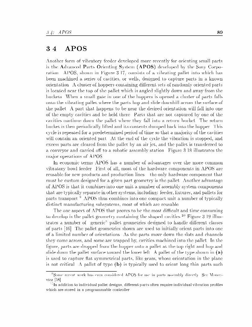
��� APOS ��
��� APOS
Another form of vibratory feeder developed more recently for orienting small partsis the Advanced Parts Orienting System APOS� developed by the Sony Corpo�ration� APOS� shown in Figure ��� � consists of a vibrating pallet into which hasbeen machined a series of cavities� or wells� designed to capture parts in a knownorientation� A cluster of hoppers containing di�erent sets of randomly oriented partsis located near the top of the pallet which is angled slightly down and away from thebuckets� When a small gate in one of the hoppers is opened a cluster of parts fallsonto the vibrating pallet where the parts hop and slide downhill across the surface ofthe pallet� A part that happens to be near the desired orientation will fall into oneof the empty cavities and be held there� Parts that are not captured by one of thecavities continue down the pallet where they fall into a return bucket� The returnbucket is then periodically lifted and its contents dumped back into the hopper� Thiscycle is repeated for a predetermined period of time so that a majority of the cavitieswill contain an oriented part� At the end of the cycle the vibration is stopped� andexcess parts are cleared from the pallet by an air jet� and the pallet is transferred toa conveyor and carried o� to a robotic assembly station� Figure ���� illustrates themajor operations of APOS�
In economic terms APOS has a number of advantages over the more commonvibratory bowl feeder� First of all� most of the hardware components in APOS arereusable for new products and production lines � the only hardware component thatmust be custom designed for a given part geometry is the pallet� Another advantageof APOS is that it combines into one unit a number of assembly system componentsthat are typically separate in other systems� including� feeder� �xtures� and pallets forparts transport� APOS thus combines into one compact unit a number of typicallydistinct manufacturing subsystems� most of which are reusable�
The one aspect of APOS that proves to be the most di�cult and time consumingto develop is the pallet geometry containing the shaped cavities�� Figure ���� illus�trates a number of �generic� pallet geometries designed to handle di�erent classesof parts ���� The pallet geometries shown are used to initially orient parts into oneof a limited number of orientations� As the parts move down the slots and channelsthey come across� and some are trapped by� cavities machined into the pallet� In the�gure� parts are dropped from the hopper onto a pallet at the top right and hop andslide down the pallet surface toward the lower left� A pallet of the type shown in a�is used to capture �at symmetrical parts� like gears� whose orientation in the planeis not critical� A pallet of type b� is typically used to orient long thin parts such
Some recent work has even considered APOS for use in parts assembly directly� See Monce�vicz �����
�In addition to individual pallet designs di�erent parts often require individual vibration pro�leswhich are stored in a programmable controller�
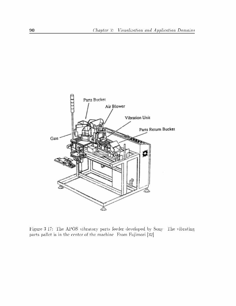
� Chapter �� Visualization and Application Domains
Figure ��� � The APOS vibratory parts feeder developed by Sony� The vibratingparts pallet is in the center of the machine� From Fujimori �����
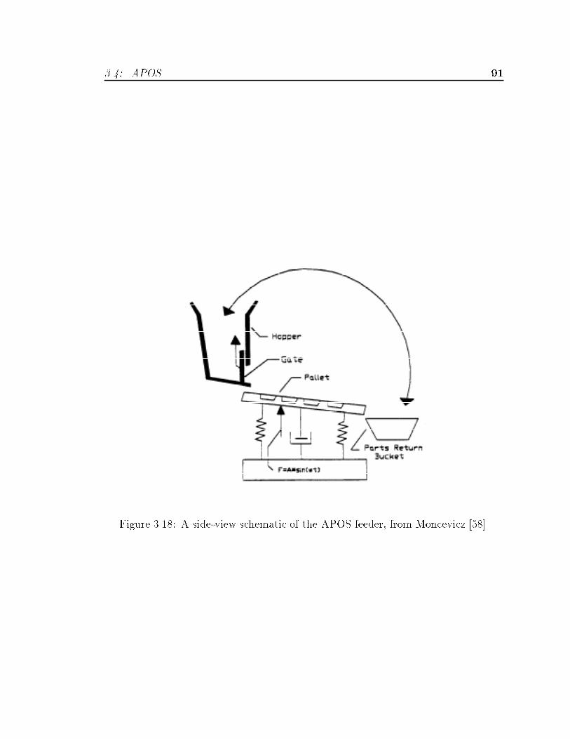
��� APOS ��
Figure ����� A side�view schematic of the APOS feeder� from Moncevicz �����

�� Chapter �� Visualization and Application Domains
as screws and springs that slide into the slots in a preferred orientation� A palletlike c� is the most common type and is typically used for less symmetrical partswhich fall into the �saw�tooth� valley and against the vertical wall in one of a limitednumber of orientations� similar to a bowl feeder track� And �nally� a pallet of typed� is used to orient parts that� after falling into one of the cavities� might blockthe �ow of following parts� It is expected that parts in the correct orientation willfall into a cavity and remain there whereas parts in the wrong orientation may fallpartially into a cavity� but should eventually bounce back out again� Characteristicsthat are desirable for an APOS pallet include�
�� the ability to trap only those parts that are in a desired con�guration�
�� the ability to hold trapped parts stably after the feeding operation� i�e� afterthe vibration has been stopped� while the pallet is unloaded and transferred tothe assembly station� and
�� the pallet provides access to parts by a robot gripper so the part may be reliablygrasped and removed from the pallet for assembly�
Comparison of these characteristics with the vibratory bowl feeder and �xture ex�amples suggests a considerable degree of functional overlap with APOS�
Like the vibratory bowl feeder� the function of APOS can be viewed in terms ofa �lter on part motions� Parts moving along the pallet surface interact with palletfeatures like those shown in Figure ���� and undergo di�erent classes of motionsdepending on the characteristic constraints imposed by those interactions� As before�we identify two motion classes� accept and reject� In the APOS example� however�the accept motion consists of a motion termination� or trapping motion� in whichthe part is stopped and held in the desired con�guration� while the reject motionfor a part consists of all other motions where the part continues across the palletsurface and into the return basket� Interestingly� the characteristics of the accept andreject motion classes for APOS are the reverse of those for the vibratory bowl feeder�Figure ��� illustrates a motion constraint metaphor for APOS� which is identicalto that of the bowl feeder except that the multiple output motions are the rejectmotions� and the single accept motion is� in essence� a null motion corresponding tothe part being contained within the vicinity of a goal region into which it will settlewhen the vibratory motion is stopped�
Depending on the type of part and pallet used� the hopping motions of the �Dparts on an APOS pallet are not always planar in a general sense� Parts droppedonto a pallet such as Figure ���� b� are constrained to move within narrow slotsso that the resulting motions all occur in more or less a vertical plane� Flat partssuch as gears� plates� brackets� levers� etc� that are dropped onto pallets such asFigure ���� a�� c� or d�� move more or less in the plane of the pallet and can oftenbe viewed as planar sliding motions with minimal vertical motion� similar to vibratory

��� APOS ��
(a) (b)
(c) (d)
Figure ����� A taxonomy of four �generic� APOS feeding pallets�
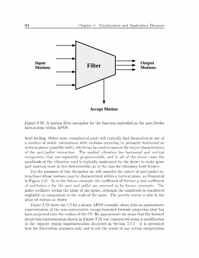
�� Chapter �� Visualization and Application Domains
Filter OutputMotions
InputMotions
Accept Motion
Figure ���� A motion �lter metaphor for the function embodied in the part�feederinteractions within APOS�
bowl feeding� Other more complicated parts will typically �nd themselves in one ofa number of stable orientations with motions occurring in primarily horizontal orvertical planes �possibly both�� which can be used to capture the major characteristicsof the part�pallet interaction� The applied vibration has horizontal and verticalcomponents that are separately programmable� and in all of the above cases theamplitude of the vibration used is typically moderated by the desire to make grosspart motions more or less deterministic� as in the case for vibratory bowl feeders�
For the purposes of this discussion we will consider the subset of part�pallet in�teractions whose motions may be characterized within a vertical plane� as illustratedin Figure ����� As in the �xture example� the coe�cient of friction � and coe�cientof restitution e for the part and pallet are assumed to be known constants� Thepallet oscillates within the plane of the �gure� although the amplitude is considerednegligible in comparison to the scale of the parts� The gravity vector is also in theplane of motion as shown�
Figure ���� shows the CS for a planar APOS example� along with an approximaterepresentation of the non�conservative energy�bounded forward projection that hasbeen projected onto the surface of the CS� By approximate we mean that the forwardprojection representation shown in Figure ���� was constructed using a modi�cationof the support region implementation discussed in Section ������ It is presentedhere for illustration purposes only and is not the result of any actual computation

��� APOS ��
g
A0 sin ω t
c.g.
X
Y
Figure ����� A planar model of a part and a vibrating APOS pallet�
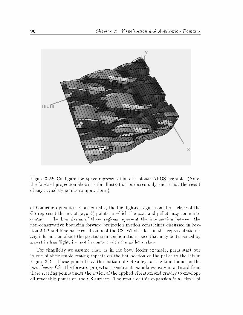
�� Chapter �� Visualization and Application Domains
Figure ����� Con�guration space representation of a planar APOS example� �Note�the forward projection shown is for illustration purposes only and is not the resultof any actual dynamics computations��
of bouncing dynamics� Conceptually� the highlighted regions on the surface of theCS represent the set of �x� y� �� points in which the part and pallet may come intocontact� The boundaries of these regions represent the intersection between thenon�conservative bouncing forward projection motion constraints discussed in Sec�tion ���� and kinematic constraints of the CS� What is lost in this representation isany information about the positions in con�guration space that may be traversed bya part in free �ight� i�e� not in contact with the pallet surface�
For simplicity we assume that� as in the bowl feeder example� parts start outin one of their stable resting aspects on the �at portion of the pallet to the left inFigure ����� These points lie at the bottom of CS valleys of the kind found on thebowl feeder CS� The forward projection constraint boundaries extend outward fromthese starting points under the action of the applied vibration and gravity to envelopeall reachable points on the CS surface� The result of this expansion is a ��ow� of

��� APOS ��
reachable points that spread down the CS valleys��� When the forward projectionregions� or �rivers� if we may further extend the metaphor� reach the set of wellson the CS corresponding to the kinematic constraints between the pallet cavitiesand parts in each of the initial orientations� then the determination of whether ornot a part is trapped in a cavity in a given orientation will depend on whether theriver is able to over�ow the well and continue to the right across the CS� For thepart� pallet� and level of applied vibration to perform properly together as a feederwill require that only one of the river �ows be stopped by a CS well while the restover�ow and continue o� the right of the pallet� In terms of motions� this means thata part starting in one orientation will be caught and held in the cavity� whereas partsstarting in other orientations will eventually bounce out of the cavity and continueacross the pallet���
We should note that the above requirements on the nature and extent of the for�ward projections on the CS for a successful APOS design are very conservative� Forexample� it is possible that if the forward projections over�owed all of the cavities ineach valley of the CS that parts would still be captured in some of those orientations�The forward projection over�owing a cavity simply means that it is possible for apart in that orientation to leave the cavity� A more detailed model might contain em�bedded shells of forward projections� each with an associated probability that a partmay reach the set of contacts contained within that shell� Of course� such a modelwould be considerably more complex than the existing �unimplemented� forwardprojection model� As noted earlier� much work remains to be done in implementingnon�conservative energy�bounded forward projection model described earlier in thischapter�
In terms of APOS design� we wish to deepen the well surrounding the desiredcon�guration relative to wells for other con�gurations so that the forward projec�tion will be trapped only by that well� The CS facets forming each of these wellsare determined by interactions between di�erent part features� and the same palletcavity features� The resulting CS facets� therefore� tend to exhibit a strong degreeof coupling� As a result� modifying a pallet feature to deepen one well will oftentend to deepen the surrounding wells� Careful attention to this coupling� as well asa considerable amount of trial and error� is required to arrive at pallet geometriesthat achieve the desired results�
��By way of analogy with the vibratory bowl feeder we can imagine collapsing these energy�bounded �rivers� down to �D space curves at which point we would expect to see a motion rep�resentation similar to that of bowl feeders� An important point to note here is that as discussedin Section ����� the exact motions of the parts on the APOS pallet will be chaotic in nature andtherefore impossible to compute exactly� The energy�bounded forward projection represents aboutthe best we can expect to do in terms of predicting the behavior of parts in this system�
��We are neglecting the e�ect of a part trapped in a cavity on subsequent parts moving across thepallet� To explicitly capture these e�ects it might be necessary to superimpose motion constraintsgenerated using a modi�ed pallet geometry consisting of the pallet and a trapped part�

�� Chapter �� Visualization and Application Domains
In addition to kinematic constraints above� the forward projections on the CSsurface will be determined by the dynamics parameters� including material propertiesof the part and pallet such as � and e� as well as the orientation of the pallet relativeto gravity �� and the orientation� amplitude and frequency of the applied vibration�� A and � respectively�
As we have seen� APOS shares many of the motion constraint characteristicsfound in the other examples discussed so far� such as the presence of valleys on theCS corresponding to stable part orientations as found in bowl feeders� and constraintwells to capture parts like those found in assemblies and �xtures� The task of de�signing an APOS system is complicated by the heavy amount of coupling presentbetween these motion constraints� which results from the fact that APOS itself com�bines so many functions into a single system� We should stress that this coupling isa re�ection of the nature of the APOS system itself and not the con�guration spacerepresentation� The representations discussed in this chapter are useful for this ap�plication precisely because they make this inherent coupling explicit� At present thecomputation of forward projection regions for actively driven vibratory systems� suchas APOS� remain an open issue for further research�
��� Summary
Figure ���� shows the planar representations of the four example domains discussedin this section� and Figure ��� shows their corresponding representations in con�g�uration space� We have noted a number of similarities between these representationsthroughout our discussion that are worth recalling here� First� we have focused aconsiderable amount of attention on the role of kinematic motion constraints rep�resented by the surface of the CS and determined by interactions between objectshapes� In the examples of assembly� parts �xtures� and the APOS feeder we sawhow some of these constraints took the form of features on the CS surface that welikened to funnels or wells that guide motions toward a speci�c state or set of states incon�guration space� In the bowl feeder and APOS examples we saw parallel valleysin the ��dimension on the CS that acted to sort and guide parts into di�erent stableorientations� In addition to kinematic constraints we saw representations of dynamicmotion constraints in terms of forward projections determined by the mechanics ofobject interaction� For the peg�in�hole assembly and vibratory bowl feeder exam�ples we were able to generate detailed representations of object motions as a set ofpaths� or trajectories� from initial states in con�guration space and constrained bycontact with the CS� For the �xture and APOS feeder examples we were unable togenerate exact motion descriptions� but instead bounded the set of reachable statesin con�guration space through which any trajectory would pass�
In addition to their similarities� the four example domains were also chosen for
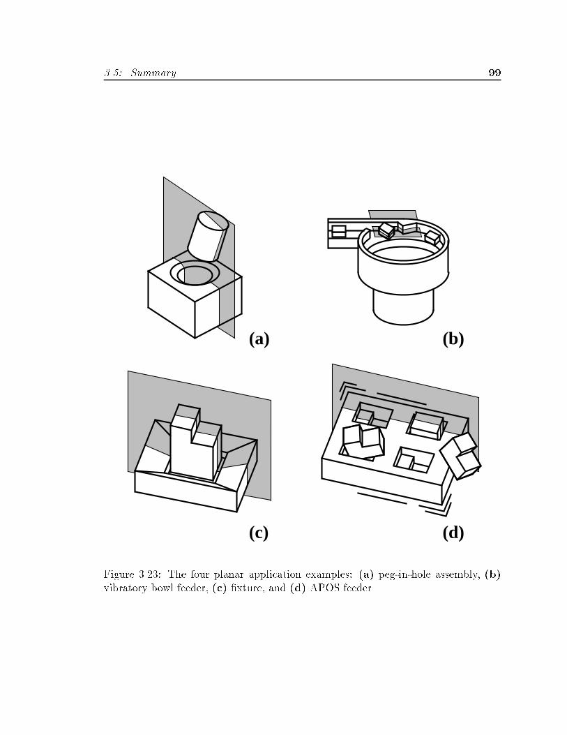
��� Summary ��
(a) (b)
(c) (d)
Figure ����� The four planar application examples� a� peg�in�hole assembly� b�vibratory bowl feeder� c� �xture� and d� APOS feeder�
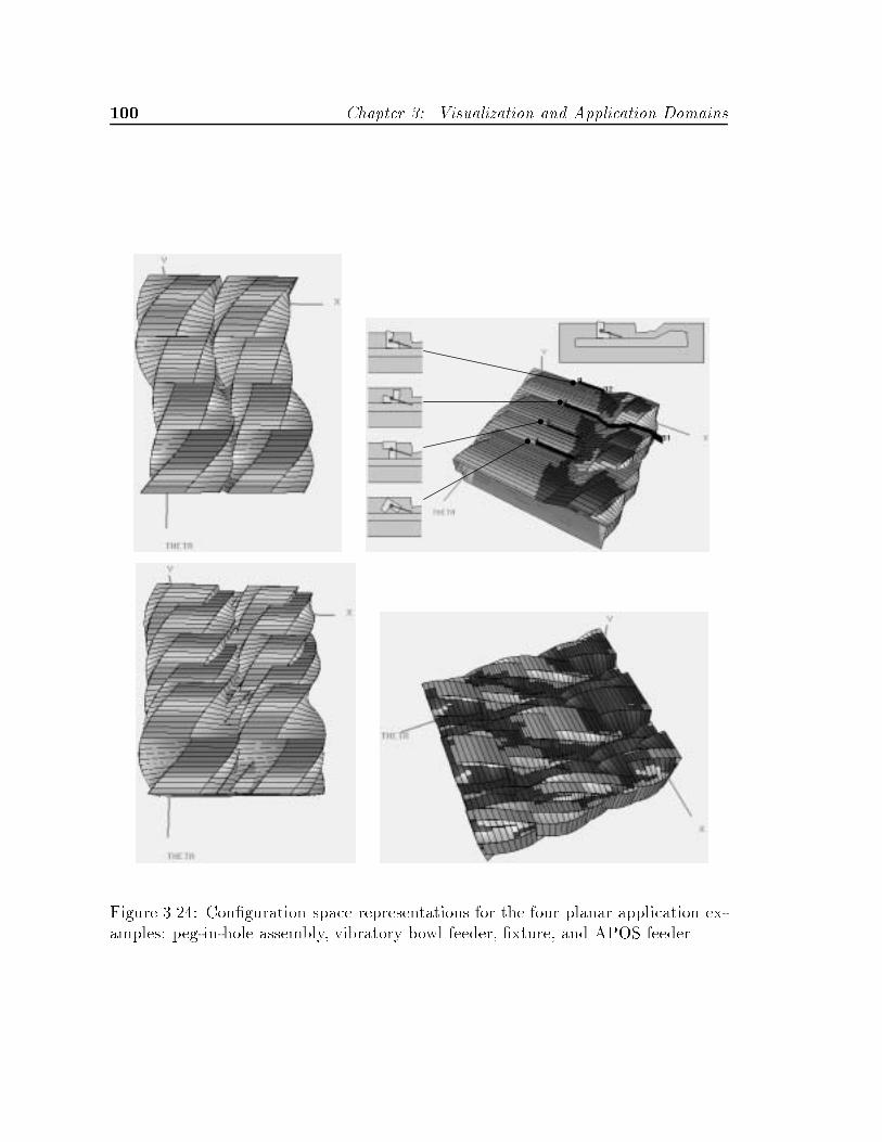
� Chapter �� Visualization and Application Domains
Figure ���� Con�guration space representations for the four planar application ex�amples� peg�in�hole assembly� vibratory bowl feeder� �xture� and APOS feeder�
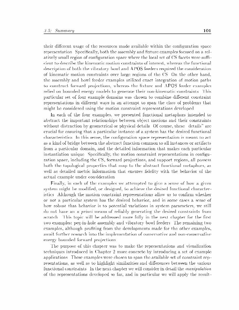
��� Summary ��
their di�erent usage of the resources made available within the con�guration spacerepresentation� Speci�cally� both the assembly and �xture examples focused on a rel�atively small region of con�guration space where the local set of CS facets were su��cient to describe the kinematic motion constraints of interest� whereas the functionaldescription of both the vibratory bowl and APOS feeders required the considerationof kinematic motion constraints over large regions of the CS� On the other hand�the assembly and bowl feeder examples utilized exact integration of motion pathsto construct forward projections� whereas the �xture and APOS feeder examplesrelied on bounded energy models to generate their non�kinematic constraints� Thisparticular set of four example domains was chosen to combine di�erent constraintrepresentations in di�erent ways in an attempt to span the class of problems thatmight be considered using the motion constraint representations developed�
In each of the four examples� we presented functional metaphors intended toabstract the important relationships between object motions and their constraintswithout distraction by geometrical or physical details� Of course� these �details� arecrucial for ensuring that a particular instance of a system has the desired functionalcharacteristics� In this sense� the con�guration space representation is meant to actas a kind of bridge between the abstract function common to all instances or artifactsfrom a particular domain� and the detailed information that makes each particularinstantiation unique� Speci�cally� the motion constraint representations in con�gu�ration space� including the CS� forward projections� and support regions� all possessboth the topological properties that map to the abstract functional metaphors� aswell as detailed metric information that ensures �delity with the behavior of theactual example under consideration�
Finally� in each of the examples we attempted to give a sense of how a givensystem might be modi�ed� or designed� to achieve the desired functional character�istics� Although the motion constraint representations allow us to con�rm whetheror not a particular system has the desired behavior� and in some cases a sense ofhow robust that behavior is to potential variations in system parameters� we stilldo not have an a priori means of reliably generating the desired constraints fromscratch� This topic will be addressed more fully in the next chapter for the �rsttwo examples� peg�in�hole assembly and vibratory bowl feeders� The remaining twoexamples� although pro�ting from the developments made for the other examples�await further research into the implementation of conservative and non�conservativeenergy bounded forward projections�
The purpose of this chapter was to make the representations and visualizationtechniques introduced in Chapter � more concrete by introducing a set of exampleapplications� These examples were chosen to span the available set of constraint rep�resentations� as well as to highlight similarities and di�erences between the variousfunctional constraints� In the next chapter we will consider in detail the manipulationof the representations developed so far� and in particular we will apply the result�

�� Chapter �� Visualization and Application Domains
ing tools to the �rst two example domains introduced in this chapter� peg�in�holeassembly and vibratory bowl feeders�

Design
Chapter �
You can�t always get what you want��� But if you try some time� youmight �nd� you get what you need�
� M� Jagger � K� Richards� ����
In this chapter we will take the representations of function in terms of motionconstraint that were developed in the previous chapter and examine how they maybe utilized for the purposes of design� We begin by considering a number of poten�tial methods by which objects with the desired constraint characteristics might begenerated� and consider a subset of these methods that appear to be both feasibleand suitable for design� We then provide an overview of an implemented toolkit forthe design of motion constraints in the form of an interactive computer aided designenvironment� This toolkit is applied to the design of artifacts from two of the ex�ample domains in the previous chapter� vibratory bowl feeder tracks and compliantpeg�in�hole assemblies� Finally� we discuss some additional characteristics of designusing motion constraints and examine the possibility of extending the scope of thetoolkit to include fully or partially automated design methodologies�
��� The Design of Motion Constraints
The CS� forward projection and support boundary representations in con�gurationspace allow us to perform the analysis necessary to determine if a given system hasthe desired functional behavior� as was illustrated for the four examples in Section ��What we lack at this point is the ability to go the other way� that is to create artifactsthat exhibit desired functional characteristics� In this section we will consider a
��

�� Chapter � Design
number of approaches aimed at inverting motion constraints to produce shapes� Wewill examine the relationship between design parameters� that describe such things asshape� and the motion constraints that we wish to create� We will extend the scopeof functional visualization developed in the previous chapter to capture constraintson the range of admissible variations of design parameters that are consistent withchanges made to motion constraints� Finally� we will consider other forms of designoperations in addition to the variation of existing design parameters�
����� Generating Shape from Motion Constraints
We will brie�y consider a number of techniques for generating shapes from motionconstraints speci�ed in con�guration space� and evaluate both their feasibility andsuitability for shape design� Considering only kinematics for the moment� one pos�sible formulation of the design problem would be to generate a set of shapes basedon a desired set of motions and kinematic motion constraints � i�e� inverting motionconstraints to produce shape� As we have seen� the mapping from shape to kinematicmotion constraints� as described in Section ���� is mathematically well de�ned andreasonably straightforward to implement� We refer to this as the forward mappingfrom shape to kinematic motion constraints to distinguish it from the inverse pro�cess� mapping from motion constraints to a pair of shapes� We will brie�y consider afew aspects of the inverse problem in order to illustrate that� as might be expected�such a direct inversion is not possible� � We will then illustrate an approach� whichwe refer to as �apparent� inversion� that allows us to perform some limited aspectsof such an inversion under a very speci�c set of constraints�
Direct Constraint Inversion
An intuitively natural approach to consider in generating shape from motion con�straints is to construct the inverse mapping from a speci�ed set of constraints rep�resenting a desired function into shape� Unfortunately� such a direct inversion is notpossible for a number of reasons� Consider� for example� constructing an arbitraryCS similar to that in Figure ��� but in which some type A facets twist clockwisewhile others twist in the counter�clockwise direction� Although it would be possi�ble to construct a closed surface consisting of such facets� it would be impossibleto generate such a surface with any pair of polygons� It is unlikely that we wouldconstruct such an odd� and faulty� CS� Nevertheless� it serves to illustrate the pointthat there does not necessarily exist a pair of shapes that will generate an arbitrarilyconstructed surface in con�guration space� Put another way� arbitrarily speci�edconstraints may be inconsistent�
�In fact it is not even a good formulation of the design problem as we shall see shortly�

��� The Design of Motion Constraints ��
{ A
A
AB
B
B
Figure ��� A few of the in�nite number of shape pairs that produce a circularconstraint region in �x� y� con�guration space�
Another problem with the direct inversion of constraints has to do with the factthat� even for a consistent set of motion constraints in con�guration space� there aremany �potentially in�nite� shape combinations that give rise to identical constraints� the inverse mapping from constraints to shape is underconstrained� Figure ��illustrates this for the simple task of creating a circular constraint region in an �x� y�con�guration space� As we can see� there are numerous shape combinations thatinteract to produce the speci�ed constraint�
Partially Constrained Inversion
Another approach for generating shape from motion constraints that has been sug�gested by a number of researchers is to constrain the problem by �xing one of the twoobjects and use it to generate the other object pro�le so that the desired constraintsare achieved� This would be done by taking the �xed shape and sweeping it throughspace along a prede�ned motion ���� ���� The complement of the volume swept outby this motion is a second maximal shape that is guaranteed not to interfere withthe speci�ed motion � this is a necessary condition on the motion constraints� Thequestion that remains is whether or not the resulting shape provides su�cient con�
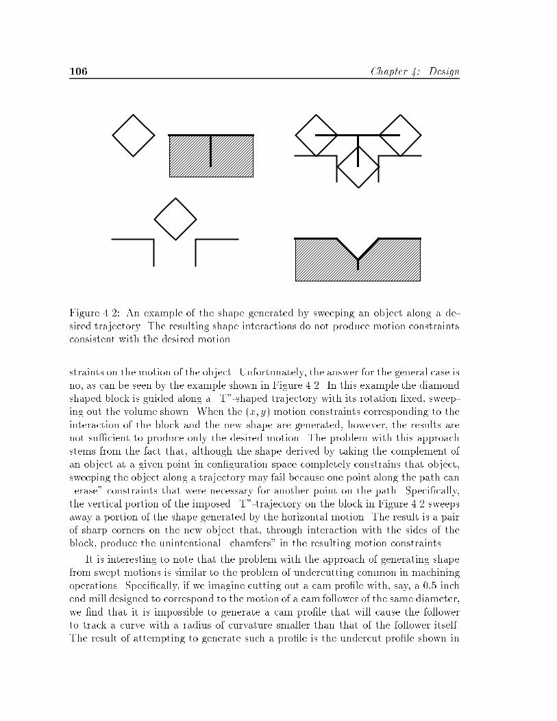
�� Chapter � Design
Figure ��� An example of the shape generated by sweeping an object along a de�sired trajectory� The resulting shape interactions do not produce motion constraintsconsistent with the desired motion�
straints on the motion of the object� Unfortunately� the answer for the general case isno� as can be seen by the example shown in Figure ��� In this example the diamondshaped block is guided along a �T��shaped trajectory with its rotation �xed� sweep�ing out the volume shown� When the �x� y� motion constraints corresponding to theinteraction of the block and the new shape are generated� however� the results arenot su�cient to produce only the desired motion� The problem with this approachstems from the fact that� although the shape derived by taking the complement ofan object at a given point in con�guration space completely constrains that object�sweeping the object along a trajectory may fail because one point along the path can�erase� constraints that were necessary for another point on the path� Speci�cally�the vertical portion of the imposed �T��trajectory on the block in Figure �� sweepsaway a portion of the shape generated by the horizontal motion� The result is a pairof sharp corners on the new object that� through interaction with the sides of theblock� produce the unintentional �chamfers� in the resulting motion constraints�
It is interesting to note that the problem with the approach of generating shapefrom swept motions is similar to the problem of undercutting common in machiningoperations� Speci�cally� if we imagine cutting out a cam pro�le with� say� a �� inchend mill designed to correspond to the motion of a cam follower of the same diameter�we �nd that it is impossible to generate a cam pro�le that will cause the followerto track a curve with a radius of curvature smaller than that of the follower itself�The result of attempting to generate such a pro�le is the undercut pro�le shown in

��� The Design of Motion Constraints ��
CS
A
B
Figure ��� An example of undercutting in a cam pro�le� which is analogous to theinconsistent motion constraints generated in Figure ���
Figure ���
Apparent Constraint Inversion
We have seen that inverting shapes from a speci�cation of desired motion constraintsis an ill�posed problem� In the case of direct inversion where both shapes were un�de�ned the inversion from motion constraints to shape was underconstrained� Con�versely� for the case of partially constrained inversion where one of the two shapeswas speci�ed� the resulting inversion was overconstrained and therefore inconsistent�Beyond these rather signi�cant limitations lies an even more fundamental problemcommon to both approaches� they assume that we already have a precise speci��cation of the motions and motion constraints that we want to achieve� As we sawin the previous chapter this is often not the case� The motion constraint represen�tations available to us provide a way of recognizing the class of motions that arerequired to produce given functional characteristics� i�e� we often only know whatwe want when we see it� The question remains� then� as to how we can achievedesired motion constraints as well as the shapes that will produce them� One answerthat we propose here is rather simple � we will take advantage of the fact that theforward mapping from shape to motion constraints is well de�ned by allowing onlycontinuous parametric variations on an existing set of design parameters�
Figure � illustrates conceptually the process of apparent inversion� Essentially�we start o� with a pair of nominal object shapes �planar polygons� from which wegenerate the CS� We provide a set of a priori mappings between features on the CS

�� Chapter � Design
UserInput
Map SelectedConstraints to
Object Features
Modify SelectedObject Features
Generate & DisplayMotion Constraints
Display
Figure �� A conceptual representation of apparent inversion from motion con�straints to shape� where a priori mappings from constraint features to shape featuresand rapid computation of the motion constraints give the illusion that motion con�straints may be inverted to produce shape�
and object features which we then use to choose shape features in the contextof motion constraints� The parameters describing these object features are thenperturbed variationally and the CS for the new objects is computed� If we are ableto� �i� map parametric perturbations that have intuitive e�ects on the CS� and �ii�perform the computation of the CS rapidly� then as far as the designer is concernedthe result is indistinguishable from a true inversion from the constraints to shape�For example� Figure �� illustrates the detailed procedure for apparent inversionof object geometry from the interactive manipulation of a contact constraint facet�Starting in the upper left of the �gure where a designer selects a point on the contactconstraint surface and displaces it vertically� the apparent inversion algorithm mapsthe selection to the appropriate shape feature �upper right�� modi�es the selectedshape feature �lower right� and recomputes the new motion constraint surface �lowerleft�� The important point to keep in mind is that the designer sees only the directmanipulation of the motion constraints� as shown in the left half of Figure ���This iterative process is carried out continuously in the background as the designermodi�es the constraints�
An important characteristic of the apparent inversion process is that after everyiteration the object shapes and the corresponding CS are guaranteed to be consistentbecause we are actually using the forward mapping from shape to constraints� whichis well de�ned� Of course� nothing is free� What we give up with apparent inversion isthe ability to make arbitrary changes to the constraints� Speci�cally� the arbitrarilyimposed a priori mapping from CS features to object features constrains the classof modi�cations that we may make to the constraints and the shapes� Our task inimplementing apparent inversion� such as in Figure �� will be to provide as complete
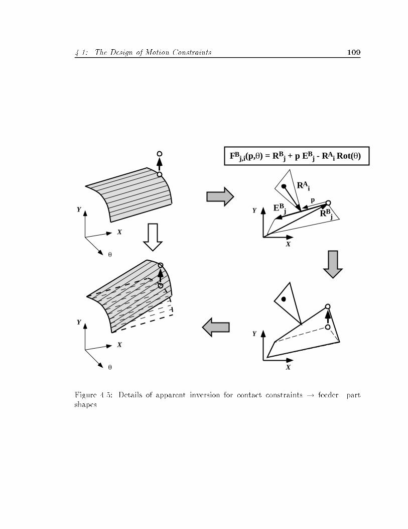
��� The Design of Motion Constraints ��
θ
X
Y
θ
X
Y
p
X
Y RBj
EBj
RAi
FBj,i(p,θ) = RBj + p EB
j - RAi Rot(θ)
X
Y
Figure ��� Details of apparent inversion for contact constraints � feeder%partshapes�

�� Chapter � Design
and �exible set of mappings as possible� The details of this process will be describedfurther in Section �� on design functions�
The motivation for manipulating design parameters by means of apparent inver�sion from motion constraints is to provide the ability to select and manipulate designparameters directly in the context of function as represented by motion constraints�The basic idea is to be able to grab one or more features on the surface of the CS andsimply push or pull them until the constraints have the desired properties� all thewhile in the background the design parameters are modi�ed so as to be consistentwith the new constraints�
����� The Space of Design Variables
In describing the changes to design parameters and the corresponding changes tomotion constraints it is useful to distinguish between the con�guration space of mo�tions and the design space of parameters that de�ne a given system� We distinguishbetween two classes of design parameters� shape parameters and dynamics param�eters� Shape parameters describe the geometry of the objects and may be take theform of a list of polygon vertices represented as �x� y� pairs� as �x� y� z� control pointsdescribing cubic polynomial surface patches� etc�� Dynamics parameters include thecoe�cients of friction and restitution� inertia� gravity and any other non�shape pa�rameters� In the same way that a point in con�guration space de�nes the state of amoving object� a point in design space de�nes all aspects of a system that may bevaried by a designer��
The design space D�
D " Pshape � Pmaterials � Pdynamics � � �
Although an explicit representation of the design space would be prohibitive giventhe large number of parameters de�ning a typical system� the concept is useful whenconsidering how changes made to constraint features in con�guration space map intochanges in the set of design parameters expressed as a point in design space� In par�ticular� we are interested in the behavior of the set of motion constraints in responseto a modi�cation of one or more design parameters� A variational modi�cation madeto a selected CS feature or set of features may be viewed as an input path speci�edin con�guration space� i�e� a point or set of points selected from the surface of theCS are coerced to follow an imposed input trajectory from their original state to anewly speci�ed state� The changes made to the constraints along this imposed pathcorrespond to changes in one or more design parameters which also may be viewed
�For the moment we are neglecting design modi�cations that would add or remove parameterssuch as adding new vertices to the list of vertices de�ning a polygon� This topic will be addressedin Section ������

��� The Design of Motion Constraints ���
as a trajectory between start and end states� but in design space� Ideally� there willbe a strong correlation between the paths in the two spaces so that� as design pa�rameters are varied by means of apparent inversion� the selected motion constraintswill closely follow the desired input trajectory in con�guration space�
����� Dynamic Constraint Visualization
Visualization is important for both analysis and design� In the previous chapter wedeveloped a representation of motion constraints to visualize function from shape in�teractions� Given a speci�c design �a single point in the space of design parameters�we were able to determine if that design possessed the desired functional characteris�tics by visualization of the motion constraints� We refer to this form of visualizationas static constraint visualization because the parameters and motion constraints re�main �xed� In the process of modifying a design� whether by means of apparentinversion from motion constraints or by some other parametric manipulation tech�nique� we are interested in the way these modi�cations will a�ect the constraints� Werefer to the visualization of the relationship between parametric variations and mo�tion constraint variations as dynamic constraint visualization because� unlike staticconstraint visualization� the motion constraint �� parameter relationship is tem�poral in nature� An important aspect of dynamic constraint visualization is that ittakes us beyond simply characterizing the function corresponding to a single pointin design space and allows us to explore the neighborhood of a design�
The changes imposed on the CS by a designer are local in the sense that theyare intended to be made only to the selected CS features� However� local suchlocal changes will typically have very non�local e�ects as well� For example� eachcontact facet can be viewed as a dual in the sense that it is determined by a set ofparameters describing a pair of interacting features on two di�erent objects� as we sawin Section ������ The facet equations� derived in Section ������ may be summarizedin the following form�
FAi�j " f�eAi � v
Bj � " f�vAi � v
Ai��� v
Bj � ����
FBj�i " f�eBj � v
Ai � " f�vBj � v
Bj��� v
Ai � ����
where the shape parameters vBj and eAi represent the jth vertex and ith edge� re�spectively� of two interacting polygons� An edge eAi may be further divided into thepair of vertices vAi � vAi�� that form its endpoints� As we can see� the characteristicsof features from each of the two objects are expressed in every contact facet�
Exactly which CS features will be a�ected by a local change can be determinedfrom Equations �� and ��� For example� a single vertex vBj � of the stationarypolygon may interact with all edges eAi � �i � � n� of the moving polygon� Anychange made to vBj � say during the apparent inversion of a feature on one type A
��� Chapter � Design
contact facet� will result in simultaneous changes being made to all the other n � �type A facets in which vBj is a contacting vertex� In addition� from Equations �� and�� we see that vBj also forms one of the endpoints of both eBj�� and eBj � Therefore�all �m type B contact facets in which vBj is an endpoint parameter will also change�Therefore� modifying a single vertex on a polygon will change a total �n � �m�contact facets on the CS�� As we can see� a considerable degree of coupling existsbetween design parameters and motion constraint features that are not local to onlythe selected constraint features� Furthermore� this coupling is unavoidable given thenature of the motion constraints forming the CS� and an understanding of the natureof the coupling will be necessary when performing design since a change to a localconstraint feature on the CS will bring a number of other� potentially important� CSfeatures �along for the ride��
As an illustration of constraint coupling� Figure �� a� shows a contact facetfeature on the CS that has been selected by a designer� Variations imposed on thisfeature in con�guration space are mapped to a single vertex on the stationary polygonin design space by means of apparent inversion� As a point on the selected CS facetis moved along an �x� y� �� path in con�guration space� the corresponding changes tothe polygon vertex generated by the apparent inverse operation cause the selectedCS feature� as well as other CS features� to change as shown in Figure �� b��
We will use dynamic visualization as a tool to explore parametric coupling amongmotion constraints during design� Two properties of apparent inversion that makedynamic constraint visualization possible and useful as a design tool are�
�� Design Direction� Parametric constraint coupling tells the designer �i�what parameters to modify� and �ii� which way to go �locally� in design spacein order to achieve the desired motion constraints in con�guration space�
�� Consistency Check� The consistency inherent in the forward mapping con�strains the designer to making changes that are possible in the context of ma�nipulating motion constraints�
These properties satisfy the necessary and su�cient conditions for getting what youwant in a design as well as providing us with the ability to perform �what if� exper�iments that are a necessary part of the iteration process in interactive design�
A crucial component in dynamic visualization is the ability to modify and re�construct motion constraints quickly so that the information contained within therelative rates of change among constraints to parametric modi�cations is accessibleto the designer� This will require the ability to compute and display the CS and
�Following a similar line of reasoning changes made to facets also produce changes in the otherCS features� edges and vertices� Edges are duals composed of facets and vertices are tripletscomposed of edges� As a result small changes to shape will change facets edges and vertices thushaving a potentially profound e�ect on the overall topology of the CS�
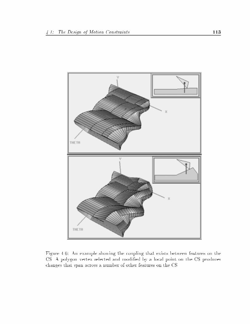
��� The Design of Motion Constraints ���
Figure ��� An example showing the coupling that exists between features on theCS� A polygon vertex selected and modi�ed by a local point on the CS produceschanges that span across a number of other features on the CS�

��� Chapter � Design
other motion constraint representations in near real time so that the gap betweenmodi�cation and constraint generation is seamless� For the rest of this chapter weshall assume such computational tools exist� Section ����� summarizes the kinds ofcomputational structures� assumptions and optimizations necessary to achieve thisgoal�
����� Topological vs� Parametric Modi�cations
In broad terms� the goal of designing motion constraints is to be able to generatemotions� or classes of motions� by means of motion constraints� So far we havedescribed a set of ideas� and some tools� that allow us to manipulate the parametersof existing motion constraints� Is this all we can do�
Parametric modi�cations may be applied only to those parameters that have al�ready been de�ned� i�e� an existing �xed set of vertices describing a polygon� Fivevertices will always describe a �ve sided polygon� no matter what values their pa�rameters may take� Therefore� an operation such as apparent inversion only allowsus to move around within a design space of �xed dimension and topology� Topolog�ical modi�cations� by which we mean changes to the size and topology of the designspace� introduce new design parameters �or eliminate old ones� and fundamentallychange the class of artifacts that may be generated� For example� generating newshapes by sweeping an object along a �xed path in con�guration space� discussed inSection ����� is a topological modi�cation� As we noted in Section ����� we cannotin general guarantee that the constraints produced by such a topological modi�ca�tion will be consistent with the intended motion� There are� however� some sweptmotion operations where this may be done consistently� one of which will be dis�cussed in Section ����� There are still other topological design operations that maybe performed consistently outside the context of constraint inversion� For example�the initial speci�cation of nominal designs upon which parametric modi�cations willbe used to iteratively arrive at a suitable design� Such nominal designs may begenerated or selected from a taxonomy of possibilities� as discussed in Section ���
Such topological modi�cations are attractive because they allow us the luxury of�jumping around� within and between multiple design spaces� as opposed to movingvariationally within a �xed design space that may� or may not� contain a valid solutionpoint� At the same time� we have already seen how local changes to a few existingparameters in a �xed design space may have signi�cant non�local e�ects on themotion constraints in con�guration space� We can only imagine what e�ect addingand deleting whole sets of parameters will have�
Comparing the relative strengths and weaknesses of parametric and topologicalmodi�cations of motion constraints we have�
Parametric Modi cations�
�� The ability to generate shapes from constraints consistently�

��� The Design of Motion Constraints ���
�� The ability to explore the neighborhood of a point in design space and to observecoupling between parameters and motion constraints�
�� Limited to varying existing parameters that correspond to only one class ofdesigns�
�� Constrained to making incremental motions in a �xed design space� Suitabledesigns may be �distant� from a given nominal design� and a solution may notexist within the given set of design parameters�
�� Reliance on the expected smoothness of design space during variational modi��cations� it is possible that for some cases a suitable design may exist onlywithin a very small region that could be bypassed while varying parameters�
Topological Modi cations�
�� Potentially a great deal of �exibility in exploring di�erent design possibilitiesencompassing many classes of designs �i�e� many design spaces��
�� The ability to �jump� between designs that are distant in terms of designparameters� or are not contained within the same design space�
�� Di�cult �often impossible� to perform consistently in the context of invertingmotion constraints�
�� A very limited set of viable design techniques exists for a few application domains�
�� Adding and removing design variables� or otherwise changing the topology ofthe design space� can make it di�cult to close in on a viable design� Jumpingaround within a design space may cause us to miss potentially valid designs�and generally makes a methodical search of possible designs di�cult to perform�Adding design variables invariably increases the dimension of the design space�also adding to the overall complexity of the design task�
As we can see� the strengths and weaknesses of parametric and topological modi��cations are more or less complementary in nature� Basically� we would like as much�exibility as possible while at the same time control the complexity that we mustdeal with� This suggests that a good design strategy would be to combine the bestof both approaches wherever possible� Speci�cally� we will want to take advantageof the �exibility of topological modi�cations early on in a design to �jump� amongpossible nominal design topologies until we �nd what appears to be a promising classof designs� Then� when we are near what we hope is feasible design� we may moremethodically explore the local parameter space for possible solutions� Section ���describes one methodology appropriate for designing vibratory bowl feeders�
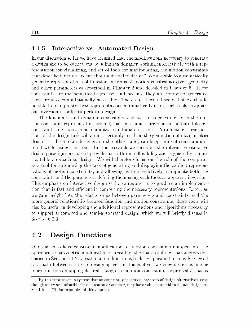
��� Chapter � Design
����� Interactive vs� Automated Design
In our discussion so far we have assumed that the modi�cations necessary to generatea design are to be carried out by a human designer working interactively with a rep�resentation for visualizing� and set of tools for manipulating� the motion constraintsthat describe function� What about automated design� We are able to automaticallygenerate representations of function in terms of motion constraints given geometryand other parameters as described in Chapter � and detailed in Chapter �� Theseconstraints are mathematically precise� and because they are computer generatedthey are also computationally accessible� Therefore� it would seem that we shouldbe able to manipulate these representations automatically using such tools as appar�ent inversion in order to perform design�
The kinematic and dynamic constraints that we consider explicitly in the mo�tion constraint representation are only part of a much larger set of potential designconstraints� i�e� cost� machinability� maintainability� etc�� Automating these por�tions of the design task will almost certainly result in the generation of many uselessdesigns�� The human designer� on the other hand� can keep more of constraints inmind while using this tool� In this research we focus on the interactive�iterativedesign paradigm because it provides us with more �exibility and is generally a moretractable approach to design� We will therefore focus on the role of the computeras a tool for automating the task of generating and displaying the explicit represen�tations of motion constraints� and allowing us to interactively manipulate both theconstraints and the parameters de�ning them using such tools as apparent inversion�This emphasis on interactive design will also require us to produce an implementa�tion that is fast and e�cient in computing the necessary representations� Later� aswe gain insight into the relationships between parameters and constraints� and themore general relationship between function and motion constraints� these tools willalso be useful in developing the additional representations and algorithms necessaryto support automated and semi�automated design� which we will brie�y discuss inSection ������
��� Design Functions
Our goal is to have consistent modi�cations of motion constraints mapped into theappropriate parametric modi�cations� Recalling the space of design parameters dis�cussed in Section ����� variational modi�cations to design parameters may be viewedas a path between states in design space� In this context� we view design as one ormore functions mapping desired changes to motion constraints� expressed as paths
�By the same token a system that automatically generates large sets of design alternatives eventhough many are infeasible for one reason or another may have value as an aid to human designers�See Ulrich ���� for examples of this approach�
��� Design Functions ���
imposed by a designer on a representation of motion constraint features� into para�metric changes represented as a path in design space� More speci�cally� design func�tions are mappings from user inputs that �i� select� and �ii� modify the appropriatedesign parameters in the context of motion constraint modi�cations�
Although the above description implies that design functions are intended purelyfor modi�cation of existing parameters� we may expand the notion of design func�tions to include those topological modi�cations to motion constraints that may beperformed consistently� In this section we will examine examples of both paramet�ric and topological design functions� We will �rst consider parametric functions toimplement apparent inversion for two forms of motion constraint representations�contact facets and planar support constraints� We will then describe a topologicaldesign operator for generating classes of support polygon geometries and discuss whyit may be implemented consistently�
����� Apparent Inversion of Motion Constraints
There are three distinct functional components of apparent inversion from motionconstraints�
�� Parameter selection� Select parameter�s� that are to be varied from theconstraint representations�
�� Input mapping� Map the designer�s intended modi�cation to the selectedparameters into a path in �x� y� �� con�guration space��
�� Parametric mapping� Map the �x� y� �� path to a path in design space� specif�ically to the selected parameter�s�� by inverting the corresponding constraintexpressions�
More precisely� these operations may be expressed in terms of the following functions�
F select�P
�x�y�� CS � FA�B
�� s ����
where P�x�y�� CS is a point selected from the surface of the facet FA�B� and s is a
parameter or set of parameters from the facet�s describing equation� For the inputmapping� we have�
F input �Pinput�� P�x�y�� CS ���
�Input mapping is an artifact of the type of input device used� Typically the input will in theform of an o�set in the screen coordinates of a cursor via a mouse� It is necessary to map sucha two variable input into a motion in the three�dimensional con�guration space� If a three d�o�f�input device is used then the input mapping function may be unnecessary�
��� Chapter � Design
where Pinput is an input path in whatever space the designer interacts with the
constraint representations� and P�x�y�� CS is the corresponding path in con�guration
space� And �nally we have�
Fmodify�s�P�x�y��
CS
���vpolygoni � s� f���vpolygoni �
�����
which applies the input path in con�guration space to the selected parameters� whichare assumed here to consist of polygon vertices�
The above functions are designed to operate on parameters describing polygongeometry in terms of �x� y� vertices� and motion constraints represented in �x� y� ��con�guration space� In this research we have developed and implemented speci�capparent inversion functions for two constraint representations� the contact facetsof the CS and the support transition boundaries on the surface of the CS� Theseparameters and representations were chosen because of their prominence in deter�mining the function of vibratory bowl feeders and compliant assemblies describedin the previous chapter� Similar functions could also be generated to operate onother design parameters� such as dynamics and material properties� as well as ma�nipulating parameters within the context of other constraint representations� such asthe forward projections including discrete paths and bounded energy regions� Suchadditional design functions have not been detailed or implemented in this report�
Inversion of Contact Facet Constraints
The kinematic constraint representations to be manipulated from the CS are theindividual contact facet equations �� and �� discussed in Section ����� and derivedin detail in Section ������ To modify a contact facet� the designer selects a point onthe surface of a facet� The selected point is mapped to a polygon vertex by meansof the selection function given by�
F selectCS
�P
�x�y�� CS � FA�B
�" v
A�Bi � FA�B
where P �x�y�� CS and FA�B are the selected point and facet as described in Equation ���
and the selected parameter s " vA�Bi � FA�B is a vertex from one of the two polygons
forming the facet� By default� the edge vertex closest to the �x� y� component of the
selected P �x�y�� CS point is chosen� Therefore� for a type A facet� the vertex will be from
polygon A� and vise versa� This a priori selection is� of course� totally arbitrary andcould be user selected�
The input mapping function is given by�
F inputCS �Pinput� " ��x� y�
where Pinput is a path in the form of an o�set in the screen coordinates of a cursor
moved by a mouse� The � component of P�x�y�� CS computed from F select
CS �� is used to
��� Design Functions ���
de�ne an �x� y� plane through that point� As the mouse is moved� the intersection of aline projected into con�guration space from the mouse screen coordinates determinesthe corresponding o�set ��x� y� representing the path P�x�y��
CS in con�guration space�
Finally� the inverse mapping function is�
FmodifyCS
�vA�Bi � ��x� y�
�" v
A�Bi �
���x� y� if FB
�Rot�������x� y� if FA
where� depending on the type of polygon to which each vertex corresponds� the o�set��x� y� is added to the selected vertices vA�Bi with or without being mapped to theappropriate � orientation by Rot������ The purpose of the �Rot����� mapping is toensure that variations to polygon A vertices cause any selected points on the type Acontact facets to follow the input path ��x� y�� Multiple vertices may be selectedwith F select
CS �� before invoking the function FmodifyCS ���
In Section ���� we discussed the inherent coupling between modi�cations madeto a single polygon vertex and the resulting changes to a number of contact facetsin the CS� Given the speci�cation of the above design functions� what more canwe say about the speci�c nature of this coupling during apparent inversion� As wenoted earlier� contact facets are formed by the interaction of an edge feature of onepolygon and a vertex of the other� From the inverse mapping function Fmodify
CS �� wecan see that a variation of ��x� y� applied to a vertex of the stationary polygon B willshift the portion of each facet containing that vertex� either as a contacting vertexor as the endpoint of a contacting edge� by a constant amount� More importantly�this shift will be invariant in �x� y� across the range � " � �� A variation of��x� y� applied to a vertex of the moving polygon A� however� will produce an o�setin con�guration space whose �x� y� orientation varies as a function of �� speci�cally�Rot�������x� y�� The resulting change will be in the form of an expanded �orcontracted� helix� Figure � illustrates these e�ects on a space curve describing avertex�vertex contact between polygons in �x� y� �� con�guration space to an �x� y�o�set in the moving polygon A�s vertex and to the stationary polygon B�s vertex�
The space curve formed by the vertex�vertex contact illustrated in Figure � is equivalent to the adjacency boundary between two facets� The e�ect that theabove transformations will have on an entire contact facet formed by a vertex�edgecontact will depend on whether the vertex being modi�ed is the contact vertex or anendpoint of the contact edge� Figure �� illustrates the e�ects for the modi�cationto a moving polygon A vertex that is a� the contact vertex� b� an edge endpointvertex� and for the modi�cation to a stationary polygon B vertex that is c� thecontact vertex� and d� an edge endpoint vertex� We note that by a priori mapping
a selected point P�x�y�� CS from a facet FA�B to an endpoint vertex v
A�Bi on a polygon
edge� we are constraining the designer to making only the modi�cations shown inFigure �� b� and d��
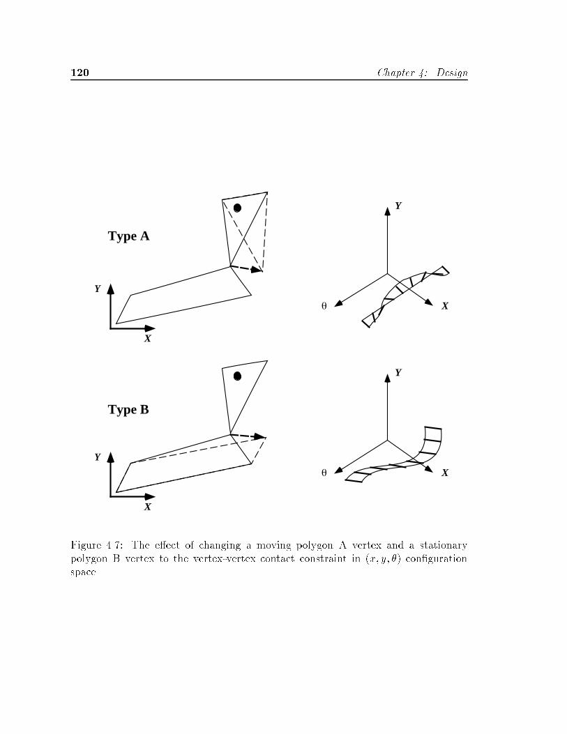
�� Chapter � Design
θ X
Y
X
Y
X
Y
θ X
Y
Type A
Type B
Figure � � The e�ect of changing a moving polygon A vertex and a stationarypolygon B vertex to the vertex�vertex contact constraint in �x� y� �� con�gurationspace�

��� Design Functions ���
X
Y
X
Y
θ
X
Y
X
Y
θ
X
Y
θ
X
Y
θ
X
Y
X
Y
(a)
(b)
(c)
(d)
Figure ��� The e�ect of changing a moving polygon A vertex that is a� the contactvertex� b� an edge endpoint vertex� and a stationary polygon B vertex that is c�the contact vertex� and d� an edge endpoint vertex�
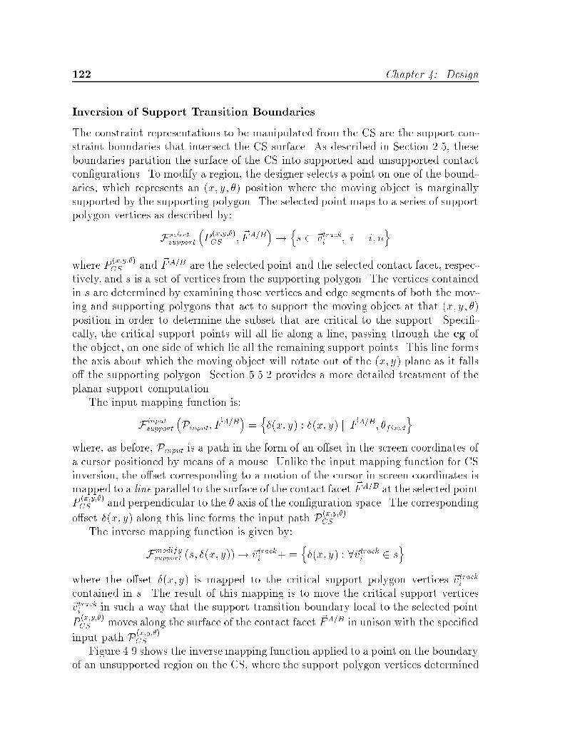
��� Chapter � Design
Inversion of Support Transition Boundaries
The constraint representations to be manipulated from the CS are the support con�straint boundaries that intersect the CS surface� As described in Section ���� theseboundaries partition the surface of the CS into supported and unsupported contactcon�gurations� To modify a region� the designer selects a point on one of the bound�aries� which represents an �x� y� �� position where the moving object is marginallysupported by the supporting polygon� The selected point maps to a series of supportpolygon vertices as described by�
F selectsupport
�P
�x�y�� CS � FA�B
��ns � vtracki � i " i� n
o
where P�x�y�� CS and FA�B are the selected point and the selected contact facet� respec�
tively� and s is a set of vertices from the supporting polygon� The vertices containedin s are determined by examining those vertices and edge segments of both the mov�ing and supporting polygons that act to support the moving object at that �x� y� ��position in order to determine the subset that are critical to the support� Speci��cally� the critical support points will all lie along a line� passing through the cg ofthe object� on one side of which lie all the remaining support points� This line formsthe axis about which the moving object will rotate out of the �x� y� plane as it fallso� the supporting polygon� Section ����� provides a more detailed treatment of theplanar support computation�
The input mapping function is�
F inputsupport
�Pinput� F
A�B�"n��x� y� � ��x� y� k FA�B� �fixed
owhere� as before� Pinput is a path in the form of an o�set in the screen coordinates ofa cursor positioned by means of a mouse� Unlike the input mapping function for CSinversion� the o�set corresponding to a motion of the cursor in screen coordinates ismapped to a line parallel to the surface of the contact facet FA�B at the selected pointP
�x�y�� CS and perpendicular to the � axis of the con�guration space� The corresponding
o�set ��x� y� along this line forms the input path P�x�y�� CS �
The inverse mapping function is given by�
Fmodifysupport �s� ��x� y��� vtracki � "
n��x� y� � vtracki � s
o
where the o�set ��x� y� is mapped to the critical support polygon vertices vtracki
contained in s� The result of this mapping is to move the critical support verticesvtracki in such a way that the support transition boundary local to the selected point
P�x�y�� CS moves along the surface of the contact facet FA�B in unison with the speci�ed
input path P�x�y�� CS �
Figure �� shows the inverse mapping function applied to a point on the boundaryof an unsupported region on the CS� where the support polygon vertices determined
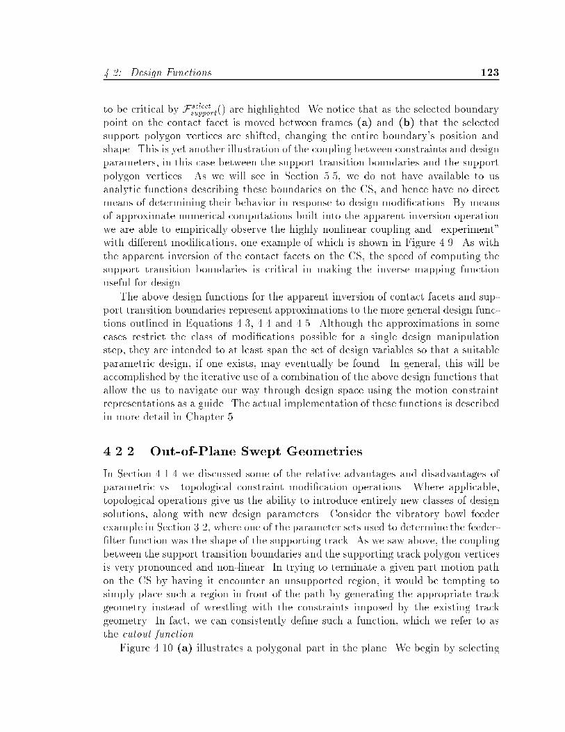
��� Design Functions ���
to be critical by F selectsupport�� are highlighted� We notice that as the selected boundary
point on the contact facet is moved between frames a� and b� that the selectedsupport polygon vertices are shifted� changing the entire boundary�s position andshape� This is yet another illustration of the coupling between constraints and designparameters� in this case between the support transition boundaries and the supportpolygon vertices� As we will see in Section ���� we do not have available to usanalytic functions describing these boundaries on the CS� and hence have no directmeans of determining their behavior in response to design modi�cations� By meansof approximate numerical computations built into the apparent inversion operationwe are able to empirically observe the highly nonlinear coupling and �experiment�with di�erent modi�cations� one example of which is shown in Figure ��� As withthe apparent inversion of the contact facets on the CS� the speed of computing thesupport transition boundaries is critical in making the inverse mapping functionuseful for design�
The above design functions for the apparent inversion of contact facets and sup�port transition boundaries represent approximations to the more general design func�tions outlined in Equations ��� � and ��� Although the approximations in somecases restrict the class of modi�cations possible for a single design manipulationstep� they are intended to at least span the set of design variables so that a suitableparametric design� if one exists� may eventually be found� In general� this will beaccomplished by the iterative use of a combination of the above design functions thatallow the us to navigate our way through design space using the motion constraintrepresentations as a guide� The actual implementation of these functions is describedin more detail in Chapter ��
����� Out�of�Plane Swept Geometries
In Section ��� we discussed some of the relative advantages and disadvantages ofparametric vs� topological constraint modi�cation operations� Where applicable�topological operations give us the ability to introduce entirely new classes of designsolutions� along with new design parameters� Consider the vibratory bowl feederexample in Section ���� where one of the parameter sets used to determine the feeder��lter function was the shape of the supporting track� As we saw above� the couplingbetween the support transition boundaries and the supporting track polygon verticesis very pronounced and non�linear� In trying to terminate a given part motion pathon the CS by having it encounter an unsupported region� it would be tempting tosimply place such a region in front of the path by generating the appropriate trackgeometry instead of wrestling with the constraints imposed by the existing trackgeometry� In fact� we can consistently de�ne such a function� which we refer to asthe cutout function�
Figure �� a� illustrates a polygonal part in the plane� We begin by selecting

��� Chapter � Design
Figure ��� Apparent inversion of a support transition boundary on the surface ofthe CS�
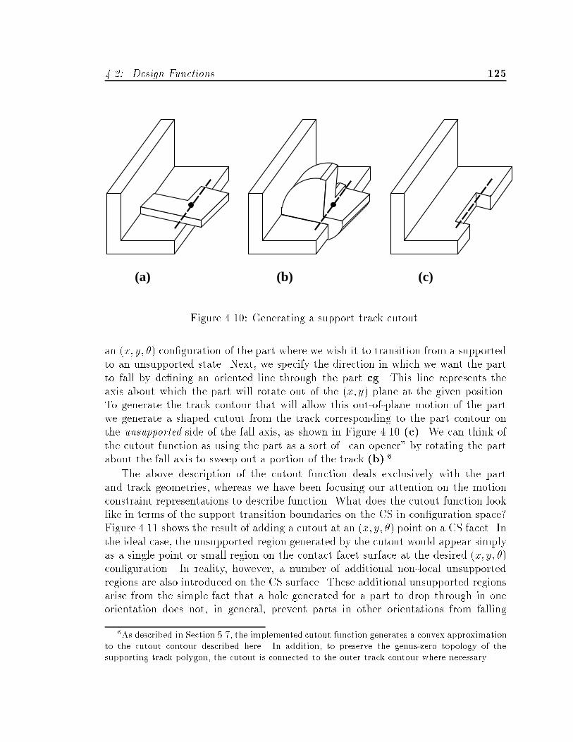
��� Design Functions ���
(a) (b) (c)
Figure ��� Generating a support track cutout�
an �x� y� �� con�guration of the part where we wish it to transition from a supportedto an unsupported state� Next� we specify the direction in which we want the partto fall by de�ning an oriented line through the part cg� This line represents theaxis about which the part will rotate out of the �x� y� plane at the given position�To generate the track contour that will allow this out�of�plane motion of the partwe generate a shaped cutout from the track corresponding to the part contour onthe unsupported side of the fall axis� as shown in Figure �� c�� We can think ofthe cutout function as using the part as a sort of �can opener� by rotating the partabout the fall axis to sweep out a portion of the track b���
The above description of the cutout function deals exclusively with the partand track geometries� whereas we have been focusing our attention on the motionconstraint representations to describe function� What does the cutout function looklike in terms of the support transition boundaries on the CS in con�guration space�Figure ��� shows the result of adding a cutout at an �x� y� �� point on a CS facet� Inthe ideal case� the unsupported region generated by the cutout would appear simplyas a single point or small region on the contact facet surface at the desired �x� y� ��con�guration� In reality� however� a number of additional non�local unsupportedregions are also introduced on the CS surface� These additional unsupported regionsarise from the simple fact that a hole generated for a part to drop through in oneorientation does not� in general� prevent parts in other orientations from falling
�As described in Section ��� the implemented cutout function generates a convex approximationto the cutout contour described here� In addition to preserve the genus�zero topology of thesupporting track polygon the cutout is connected to the outer track contour where necessary�

��� Chapter � Design
through as well� The location� number� size� and shape of these additional regionsare determined by the location and shape of the track cutout contour� which in turnis determined by the chosen �x� y� �� con�guration and fall axis orientation for thecutout� As expected� the topological modi�cations created by the cutout functionadd complexity as well as �exibility to the design task by introducing a number ofnew polygon vertices� Controlling this additional complexity while at the same timetaking advantage of the ability to introduce an unsupported region at any arbitrarylocation on the surface of the CS is the major challenge of utilizing the cutout functionas a design tool�
We noted in Section ���� that the shape created by sweeping out a part alonga desired path in con�guration space satis�ed the necessary conditions� but not thesu�cient conditions for the desired motion constraints along that path� Does thecutout function above satisfy both the necessary and su�cient conditions for produc�ing the desired motion constraints� and if so� why� We recall from Section ���� thatthe problem with the swept shape generation approach was the fact that the volumeswept out by the �xed object on one portion of the speci�ed path could eliminateshape features that were necessary to constrain the object along another portion ofthe path� as illustrated in Figures �� and ��� If we imagine the rotation of the partout of the �x� y� plane as a path in a higher dimensional con�guration space� thenonly the point corresponding to the beginning of the path is contained within thelower dimensional �x� y� �� slice of that space� As a result� the support constraintsprovided by the track at the �x� y� �� position where the out�of�plane path begins arenot a�ected by any other point along the remainder of that path� By this argument�the shape generated by the swept out�of�plane motion provides the intended motionconstraints� i�e� support constraints� at the selected �x� y� �� point� We are� how�ever� ignoring an important additional factor � we neglect the remainder of the partmotion outside the �x� y� �� plane� In particular� we could imagine a case where thehalf of the part on the supported side of the fall axis is wider than the unsupportedhalf used to generate the cutout contour� In this case� a part may rotate out of theplane as desired� but become caught in the cutout rather than falling o� the track�In this research we are assuming that the parts are thin enough compared to their�x� y� dimension that we could� if necessary� cut an additional narrow slot along thefall axis whose length exceeded the widest cross�section of the part� This slot wouldbe swept out by the part as it reached a vertical orientation and then slid downwardin the �z direction� Although an inelegant solution� such a slot would allow thepart to slide o� the track while at the same time yet be narrow enough so as not tocompromise the support characteristics of parts in other orientations in the plane�

��� Design Functions ���
Figure ���� Multiple unsupported regions generated on the CS by the cutout func�tion applied to a single �x� y� �� con�guration �indicated by the �P� in the top �gure��

��� Chapter � Design
��� A Toolkit for Visualization and Design
In this section we give a brief overview of an implemented set of tools that form a com�putational environment for visualization and design called cspace�shell� Speci��cally� we�ve selected the representations for the CS� numerically integrated forwardprojections� and unsupported regions on the CS surface� which are a subset of themotion constraint representations discussed in Chapter �� This subset was chosenbecause it will be su�cient to represent both the compliant peg�in�hole assembly andvibratory bowl feeder examples described in Section ��
����� Assumptions
Most of the following the assumptions made in computing motion constraints havebeen discussed in earlier chapters but are repeated here for completeness� Whereappropriate� we note assumptions that are unique to speci�c application domains�
� Objects are modeled as in�nitely rigid planar polygons that do not changeshape under applied loads�
� The dynamics governing object motions are assumed to be quasi�static� bodyforces due to velocities and accelerations of the objects are considered negligiblein comparison to static forces�
� Externally applied forces� such as gravity� are assumed to act through the ref�erence point of the moving object� For the vibratory bowl feeder example� weassume this point to be the object�s center of gravity cg� whereas for the com�pliant assembly example the reference point is the remote center of compliance�RCC��
� The contact between the moving object and plane of motion is assumed tobe frictionless� reaction forces occur solely between polygon boundaries in theplane of motion�
� In the vibratory feeder examples� we assume that parts move along the trackindividually� with contacts occurring only between the part and feeder wall �no stacking or bunching of parts is considered�
� Out of plane motions� such as hopping of parts on a vibratory feeder track� areassumed to be negligible in comparison to in�plane motions�
� Parameters are known exactly� and part motions are modeled as being com�pletely deterministic�

��� A Toolkit for Visualization and Design ���
����� Overview and Layout
The main functions contained within cspace�shell are�
� Interactive GUI � mouse based input via buttons� sliders� and surface pointselection�
� Geometric modeler � representation and manipulation of planar polygons�
� Motion constraint visualizer � engine for rapid computation� display� andinterrogation of motion constraint representations�
� Apparent inversion functions � parametric selection and manipulation viaconstraint representations�
� Parametric coupling visualizer � highlighting of motion constraint featurescoupled to selected polygon vertices�
� Functional veri cation � numerical simulation and animation of part mo�tions�
� UNDO� � can play with shapes and constraints without destroying existingdesigns�
� Feeder path optimizer � rendering of motion path thickness is proportionalto the probability of part entering a feeder in a given orientation� Feederspassing thicker paths have a higher average throughput�
Figure ��� shows the layout for the main interface with cspace�shell� The largewindow on the left displays the various motion constraints in �x� y� �� con�gurationspace� The viewing angle and zoom for this window are controlled by the viewbuttons in the lower left� The three smaller windows on the right are from top tobottom� the display for the moving polygon� the display for the stationary polygon�and track� if included�� and the object position and animation display window�The sliders in the bottom center control the resolution to which the approximateunsupported regions are computed on the CS� the direction of the applied force tothe moving polygon� the radius of gyration of the moving polygon� and the coe�cientof friction between the moving and stationary polygons� The two small radio buttonsabove the top right of the large motion constraint viewing window allow the user toselect between apparent inversion of �i� the contact facets forming the CS� and �ii�the support transition boundaries� The buttons across the top of the �gure controlvarious other functions including� �le I�O� mode selection� undo of last modi�cation�cutout function selection� motion path computation� and path animation� There aretwo other windows �not shown� that may be selected via the mode selection menu�The �rst is a rendering control window containing a palette of �� colors that are
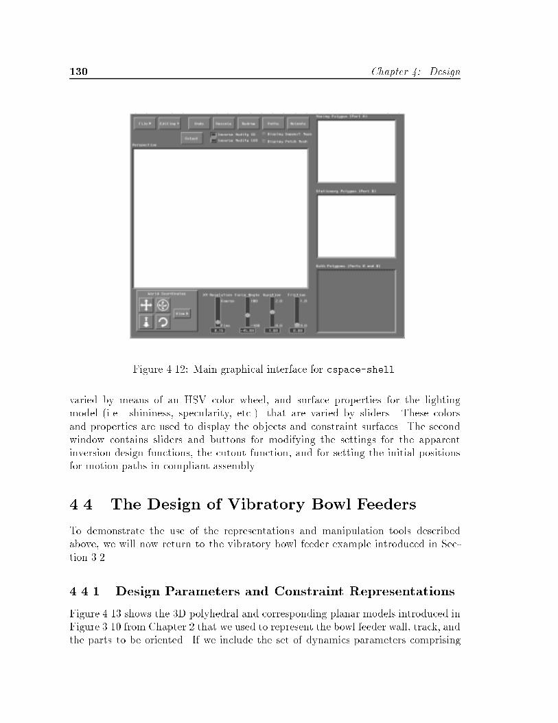
�� Chapter � Design
Figure ���� Main graphical interface for cspace�shell�
varied by means of an HSV color wheel� and surface properties for the lightingmodel �i�e� shininess� specularity� etc�� that are varied by sliders� These colorsand properties are used to display the objects and constraint surfaces� The secondwindow contains sliders and buttons for modifying the settings for the apparentinversion design functions� the cutout function� and for setting the initial positionsfor motion paths in compliant assembly�
��� The Design of Vibratory Bowl Feeders
To demonstrate the use of the representations and manipulation tools describedabove� we will now return to the vibratory bowl feeder example introduced in Sec�tion ����
����� Design Parameters and Constraint Representations
Figure ��� shows the �D polyhedral and corresponding planar models introduced inFigure ��� from Chapter � that we used to represent the bowl feeder wall� track� andthe parts to be oriented� If we include the set of dynamics parameters comprising

�� The Design of Vibratory Bowl Feeders ���
X Y
Z
X
Y
θ+
Figure ���� A polyhedral model of a portion of the feeder track near the outlet ofthe bowl �top�� and an equivalent planar model viewed from above �bottom��
the applied force and material property parameters� then we have a total of foursets of design parameters with which to work�
The degree of coupling between design parameter motion constraints thatwe illustrated in Sections ���� and ���� is not completely global or all inclusive�Rather� di�erent groups of parameters control and are controlled by di�erent motionconstraints that form a rough hierarchy� as illustrated by Figure ��� Speci�cally�
� the kinematic constraints represented by the CS are determined solely by thepart and bowl wall interactions�
� the support transition boundaries on the CS are determined by the interactionbetween the part and track �and also the bowl wall since the support regionsare intersected with the CS���
�The coupling between changes to the bowl wall and the support transition boundaries is actually
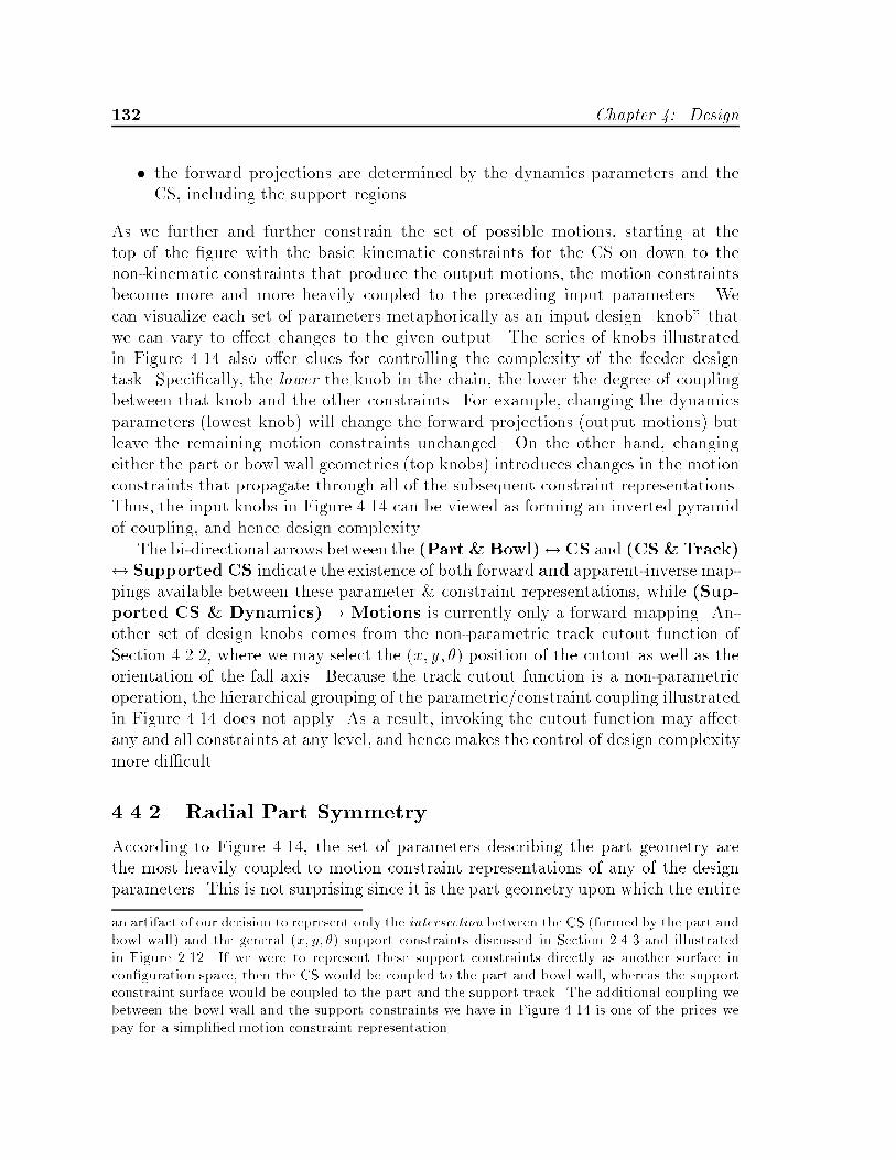
��� Chapter � Design
� the forward projections are determined by the dynamics parameters and theCS� including the support regions�
As we further and further constrain the set of possible motions� starting at thetop of the �gure with the basic kinematic constraints for the CS on down to thenon�kinematic constraints that produce the output motions� the motion constraintsbecome more and more heavily coupled to the preceding input parameters� Wecan visualize each set of parameters metaphorically as an input design �knob� thatwe can vary to e�ect changes to the given output� The series of knobs illustratedin Figure �� also o�er clues for controlling the complexity of the feeder designtask� Speci�cally� the lower the knob in the chain� the lower the degree of couplingbetween that knob and the other constraints� For example� changing the dynamicsparameters �lowest knob� will change the forward projections �output motions� butleave the remaining motion constraints unchanged� On the other hand� changingeither the part or bowl wall geometries �top knobs� introduces changes in the motionconstraints that propagate through all of the subsequent constraint representations�Thus� the input knobs in Figure �� can be viewed as forming an inverted pyramidof coupling� and hence design complexity�
The bi�directional arrows between the Part � Bowl�CS and CS � Track� Supported CS indicate the existence of both forward and apparent�inverse map�pings available between these parameter � constraint representations� while Sup�ported CS � Dynamics� � Motions is currently only a forward mapping� An�other set of design knobs comes from the non�parametric track cutout function ofSection ����� where we may select the �x� y� �� position of the cutout as well as theorientation of the fall axis� Because the track cutout function is a non�parametricoperation� the hierarchical grouping of the parametric�constraint coupling illustratedin Figure �� does not apply� As a result� invoking the cutout function may a�ectany and all constraints at any level� and hence makes the control of design complexitymore di�cult�
����� Radial Part Symmetry
According to Figure ��� the set of parameters describing the part geometry arethe most heavily coupled to motion constraint representations of any of the designparameters� This is not surprising since it is the part geometry upon which the entire
an artifact of our decision to represent only the intersection between the CS formed by the part andbowl wall� and the general x� y� �� support constraints discussed in Section ����� and illustratedin Figure ����� If we were to represent these support constraints directly as another surface incon�guration space then the CS would be coupled to the part and bowl wall whereas the supportconstraint surface would be coupled to the part and the support track� The additional coupling webetween the bowl wall and the support constraints we have in Figure ���� is one of the prices wepay for a simpli�ed motion constraint representation�
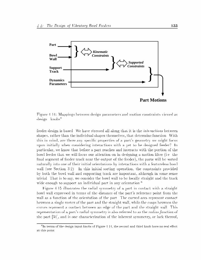
�� The Design of Vibratory Bowl Feeders ���
Part
BowlWall
SupportTrack
DynamicsParameters
Part Motions
SupportedConstraints
KinematicConstraints}
}}
Figure ��� Mappings between design parameters and motion constraints viewed asdesign �knobs��
feeder design is based� We have stressed all along that it is the interactions betweenshapes� rather than the individual shapes themselves� that determine function� Withthis in mind� are there any speci�c properties of a part�s geometry we might focusupon initially when considering interactions with a yet to be designed feeder� Inparticular� we know that before a part reaches and interacts with the portion of thebowl feeder that we will focus our attention on in designing a motion �lter �i�e� the�nal segment of feeder track near the output of the feeder�� the parts will be sortednaturally into one of their initial orientations by interactions with a featureless bowlwall �see Section ����� In this initial sorting operation� the constraints providedby both the bowl wall and supporting track are important� although in some sensetrivial� That is to say� we consider the bowl wall to be locally straight and the trackwide enough to support an individual part in any orientation��
Figure ��� illustrates the radial symmetry of a part in contact with a straightbowl wall expressed in terms of the distance of the part�s reference point from thewall as a function of the orientation of the part� The curved arcs represent contactbetween a single vertex of the part and the straight wall� while the cusps between thecurves represent a contact between an edge of the part and the straight wall� Thisrepresentation of a part�s radial symmetry is also referred to as the radius function ofthe part ���� and is one characterization of the inherent symmetry� or lack thereof�
�In terms of the design input knobs of Figure ���� the second and third knob have no real e�ectat this point�

��� Chapter � Design
of a planar object� We have seen the radius function a number of times before�although in a slightly di�erent form� Figure ��� shows a view of a CS formed by thepart in Figure ��� interacting with a portion of a straight wall� In Figure ��� weare looking along the x axis of the �x� y� �� con�guration space so that we are seeingthe y vs� � pro�le of the CS� The curved surfaces of the facets and valleys betweenthem are the radius function�
From a design point of view the part�s symmetry� as characterized by the radiusfunction� represents what we�re given to work with� Speci�cally� the cusps formedby the edge�edge contacts in Figure ���� corresponding to the edge�edge valleys onthe CS surface� are a superset of the stable initial orientations into which a part willsettle as it moves up the track� The relative heights of these cusps in the radiusfunction are a measure of the separability of the various stable part orientations� Apart whose cusps are all at nearly the same height �i�e� distance of the cg fromthe bowl wall� is nearly symmetric� and therefore its stable orientations are nearlyindistinguishable from one another as measured from the wall� A part with at leastone cusp easily distinguishable from the others� on the other hand� is more likely tobe sorted by� for example� a feeder with a simple narrowed track�
����� The Integration of PartFeeder Design
Themotion constraint representations we have developed for both analysis and designare general enough that they allow modi�cations to be made to the feeder geometry inthe same way as to the geometry of the part being fed� In fact� the tools and methodsdeveloped so far do not distinguish between feeder and part� This is signi�cantbecause� where possible� redesigning a part so as to make it easier to orient can reducethe number and complexity of required feeding devices� In addition� redesigning partsto a new model of an existing product may allow for the reuse of existing toolingand equipment�
Part redesign may also make sense for a number of other� more technical� reasons�First� as we saw in Figure ��� the part geometry directly determines each andevery motion constraint representation� from the CS to the forward projections�The central role of part geometry in the feeding operation provides a great deal of�exibility in design� In addition� the degree of radial symmetry determined by thepart geometry determines the set of initial orientations we will have to �lter� as seenin Section ���� as well as the design strategies to be employed� as we will see inSection ����
Consider the extreme case where we are trying to distinguish between stable orientations of acircular disk� The radius function for such a part would be a horizontal line indicating that �a�there were no �nite stable orientations characterized by a cusp and �b� the orientations of the partwere indistinguishable from one another�
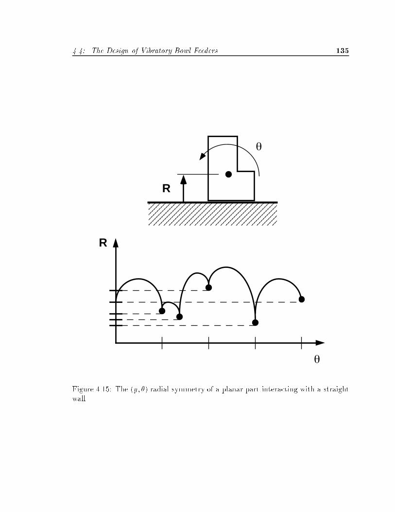
�� The Design of Vibratory Bowl Feeders ���
R
θ
θ
R
Figure ���� The �y� �� radial symmetry of a planar part interacting with a straightwall�
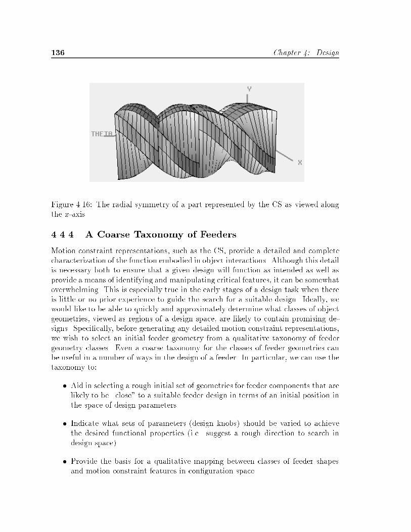
��� Chapter � Design
Figure ���� The radial symmetry of a part represented by the CS as viewed alongthe x�axis�
����� A Coarse Taxonomy of Feeders
Motion constraint representations� such as the CS� provide a detailed and completecharacterization of the function embodied in object interactions� Although this detailis necessary both to ensure that a given design will function as intended as well asprovide a means of identifying and manipulating critical features� it can be somewhatoverwhelming� This is especially true in the early stages of a design task when thereis little or no prior experience to guide the search for a suitable design� Ideally� wewould like to be able to quickly and approximately determine what classes of objectgeometries� viewed as regions of a design space� are likely to contain promising de�signs� Speci�cally� before generating any detailed motion constraint representations�we wish to select an initial feeder geometry from a qualitative taxonomy of feedergeometry classes� Even a coarse taxonomy for the classes of feeder geometries canbe useful in a number of ways in the design of a feeder� In particular� we can use thetaxonomy to�
� Aid in selecting a rough initial set of geometries for feeder components that arelikely to be �close� to a suitable feeder design in terms of an initial position inthe space of design parameters�
� Indicate what sets of parameters �design knobs� should be varied to achievethe desired functional properties �i�e� suggest a rough direction to search indesign space��
� Provide the basis for a qualitative mapping between classes of feeder shapesand motion constraint features in con�guration space�
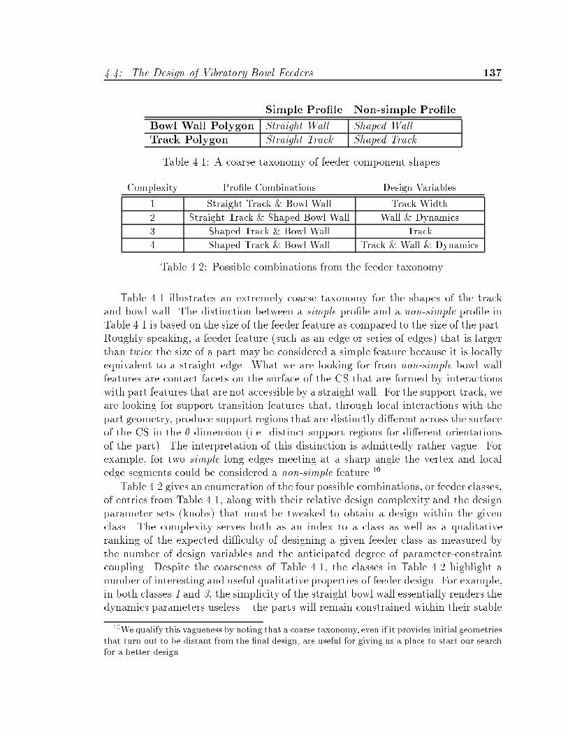
�� The Design of Vibratory Bowl Feeders ���
Simple Pro le Non�simple Pro le
Bowl Wall Polygon Straight Wall Shaped WallTrack Polygon Straight Track Shaped Track
Table ��� A coarse taxonomy of feeder component shapes�
Complexity Pro�le Combinations Design Variables
� Straight Track � Bowl Wall Track Width
� Straight Track � Shaped Bowl Wall Wall � Dynamics
� Shaped Track � Bowl Wall Track
� Shaped Track � Bowl Wall Track � Wall � Dynamics
Table ��� Possible combinations from the feeder taxonomy�
Table �� illustrates an extremely coarse taxonomy for the shapes of the trackand bowl wall� The distinction between a simple pro�le and a non�simple pro�le inTable �� is based on the size of the feeder feature as compared to the size of the part�Roughly speaking� a feeder feature �such as an edge or series of edges� that is largerthan twice the size of a part may be considered a simple feature because it is locallyequivalent to a straight edge� What we are looking for from non�simple bowl wallfeatures are contact facets on the surface of the CS that are formed by interactionswith part features that are not accessible by a straight wall� For the support track� weare looking for support transition features that� through local interactions with thepart geometry� produce support regions that are distinctly di�erent across the surfaceof the CS in the � dimension �i�e� distinct support regions for di�erent orientationsof the part�� The interpretation of this distinction is admittedly rather vague� Forexample� for two simple long edges meeting at a sharp angle the vertex and localedge segments could be considered a non�simple feature��
Table �� gives an enumeration of the four possible combinations� or feeder classes�of entries from Table ��� along with their relative design complexity and the designparameter sets �knobs� that must be tweaked to obtain a design within the givenclass� The complexity serves both as an index to a class as well as a qualitativeranking of the expected di�culty of designing a given feeder class as measured bythe number of design variables and the anticipated degree of parameter�constraintcoupling� Despite the coarseness of Table ��� the classes in Table �� highlight anumber of interesting and useful qualitative properties of feeder design� For example�in both classes � and �� the simplicity of the straight bowl wall essentially renders thedynamics parameters useless � the parts will remain constrained within their stable
�We qualify this vagueness by noting that a coarse taxonomy even if it provides initial geometriesthat turn out to be distant from the �nal design are useful for giving us a place to start our searchfor a better design�

��� Chapter � Design
Simple Pro le Non�simple Pro les
Bowl Wall �a� Straight �b� Protrusion �c� CavityTrack �d� Straight �e� Protrusion �f� Cavity
Table ��� A slightly re�ned taxonomy of feeder component shapes�
orientations as they pass along the wall� The only design variables we have availableto us in these feeder classes are those de�ning the track pro�le �class �� and itslocation relative to the bowl wall �class ��� In terms of motion constraints� we mustrely solely on modi�cations to the support regions on the CS to �lter part motions�In �class �� in particular� the success or failure of a feeder design will be determinedby varying one parameter specifying the track�bowl wall o�set� The success or failureof this class of feeder will be determined by the di�erentiability of part orientationsinherent to the part geometry� as given by the radius function in Section ���� Class �allows us to utilize detailed part geometry for the purposes of di�erentiating motionpaths only by means of varying the support interactions between the part and trackcontours� From the motion constraint representations this means that� as for class���� we can only manipulate the support transition boundaries �albeit more complexand localizable ones� on the CS surface�
Classes � and from Table �� involve interactions between a part and non�simple bowl wall features that may allow for the di�erentiation of motion pathsbeyond what is inherently given by the part geometry� Speci�cally� for class ��� wemay manipulate paths on the CS by changing �i� the dynamics� and �ii� the bowlwall pro�le to redirect the individual motion paths of the parts��� In class �� wehave the combined e�ects� and therefore complexity due to coupling� of all sets ofdesign variables� Finally� we note that both classes ��� and ��� in which the trackpro�le is non�simple� are judged more complex than simple or non�simple bowl wallpro�les because of the highly coupled and non�linear nature of the support transitionboundaries as noted in Section �����
The feeder taxonomy illustrated in Table ��� and the feeder classes derived fromit in Table ��� provide us with a reasonably coarse� �rst�cut grouping of the basicfeeder feature types we were looking for to begin the design process� One problemwith using these tables in their present form� however� is that they do not directly tiein to any particular classi�cation of the motion constraint features in con�gurationspace that we will have to use in our search for more detailed designs� To address thisshortcoming� we will generate a slightly more detailed taxonomy of feeder featuresshown in Table ��� The basic di�erence between Tables �� and �� is a minorre�nement of the term non�simple into two sub�classes denoting protrusions from
��Unfortunately in the present representation changes to the CS will also produce changes inthe supported regions on the surface of the CS� See Section ������
�� The Design of Vibratory Bowl Feeders ���
and cavities in either a track or bowl wall pro�le��� The important di�erence here isthat elements from this re�ned taxonomy may be mapped into the set of qualitativelydistinct motion constraint features in con�guration space given below� We use letterindices to the elements of Table �� to avoid confusion with the feeder classes ofTable �����
a� The straight bowl wall produces a series of parallel valleys running perpendic�ular to the � axis of the �x� y� �� con�guration space� These valleys form a�washboard��like surface made up primarily of type B contact facets� whichact to constrain and guide the naturally di�erentiated stable orientations of apart along the wall� as shown in Figure �� a��
b� A protrusion from the bowl wall produces a ridge across the surface of the CS inthe � direction of the con�guration space� shown in Figure �� b�� A ridge istypically made up of both type A and type B facets� and serves to di�erentiatemotions further than is possible with the valleys in a� because many parts of agiven path are across a single contact facet and therefore may be manipulatedby adjustments to the dynamics parameters as well as to the facets themselves�
c� A concavity in the bowl wall produces a valley across the CS surface in the �direction as shown in Figure �� c�� This valley� also consisting generally ofboth type A and type B facets also acts to di�erentiate motion paths� or insome cases may be used to combine motion paths �i�e� part reorienting��
d� A straight track pro�le �within the half�width of a part from the bowl wall� willproduce supported regions� or passes� along deeper valleys on the CS surface�as shown in Figure ��� d�� If the straight section of the track is not parallelto the straight portion of the wall� the passes will become wider or narroweralong the x direction of a CS valley�z
e� A protrusion from the track pro�le may produce isolated islands within unsup�ported regions or entire swaths of support on the CS in the � direction ofcon�guration space� as shown in Figure ��� e�� Both isolated islands andsupported swaths are rather useless alone since they are not reachable by anypaths starting outside the unsupported regions� For this reason� track protru�sions are typically combined with bowl wall protrusions to form passes acrossridges on the CS so that some di�erentiated paths are supported whereas othersare unsupported as the parts rotate and translate across the track surface�z
��Again we distinguish between simple and non�simple features based on the relative size of thefeature to a part�
��We will not bother to enumerate the nine possible combinations of the bowl wall and trackelements from Table ����

�� Chapter � Design
a�
b�
c�
Figure �� � A taxonomy of CS features in �x� y� �� con�guration space for di�erentclasses of bowl wall pro�les�
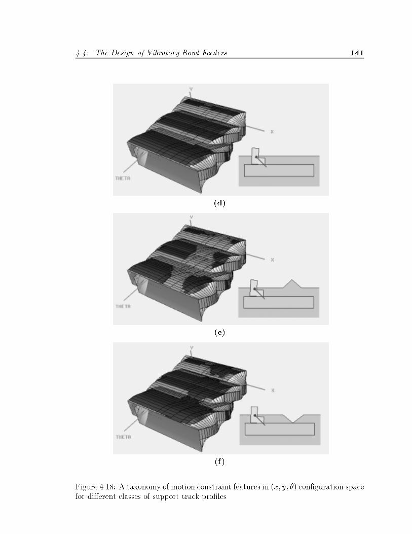
�� The Design of Vibratory Bowl Feeders ���
d�
e�
f�
Figure ���� A taxonomy of motion constraint features in �x� y� �� con�guration spacefor di�erent classes of support track pro�les�
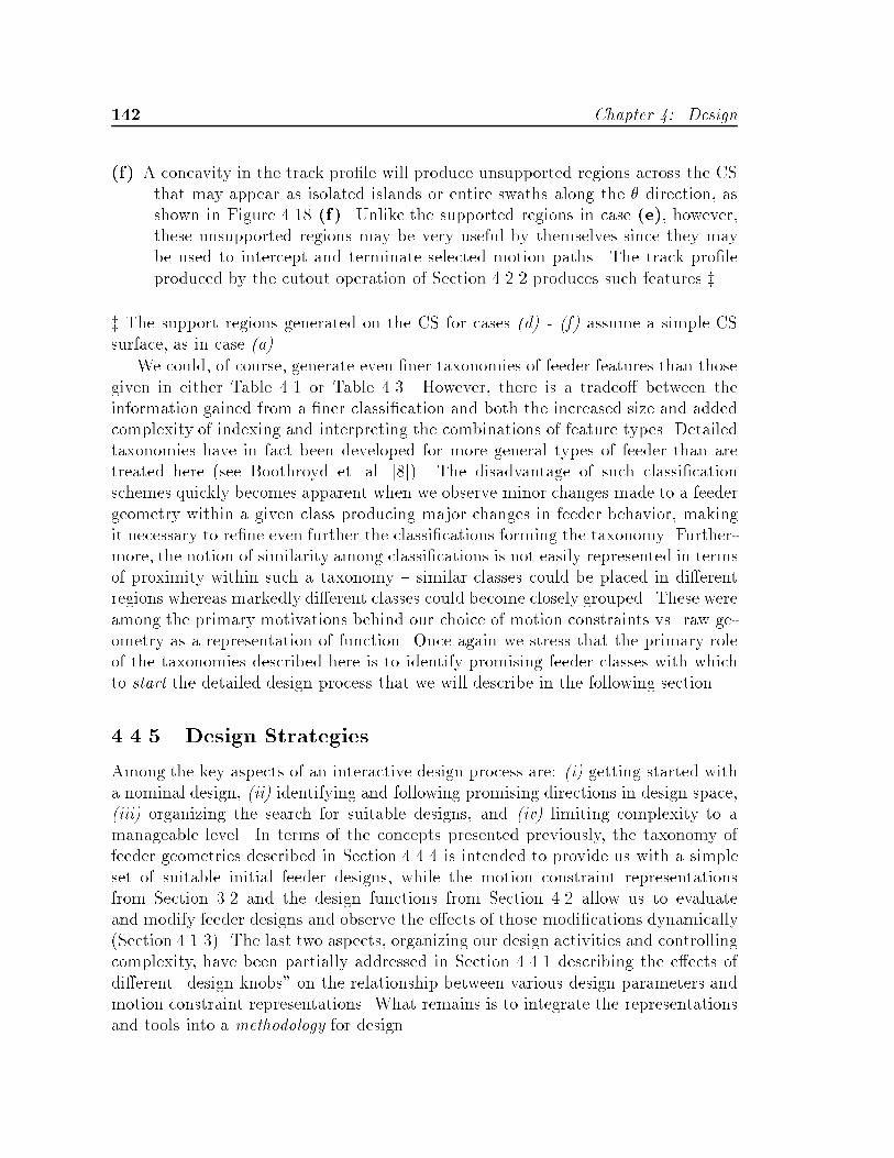
��� Chapter � Design
f� A concavity in the track pro�le will produce unsupported regions across the CSthat may appear as isolated islands or entire swaths along the � direction� asshown in Figure ��� f�� Unlike the supported regions in case e�� however�these unsupported regions may be very useful by themselves since they maybe used to intercept and terminate selected motion paths� The track pro�leproduced by the cutout operation of Section ���� produces such features�z
z The support regions generated on the CS for cases �d� � �f� assume a simple CSsurface� as in case �a��
We could� of course� generate even �ner taxonomies of feeder features than thosegiven in either Table �� or Table ��� However� there is a tradeo� between theinformation gained from a �ner classi�cation and both the increased size and addedcomplexity of indexing and interpreting the combinations of feature types� Detailedtaxonomies have in fact been developed for more general types of feeder than aretreated here �see Boothroyd et� al� ����� The disadvantage of such classi�cationschemes quickly becomes apparent when we observe minor changes made to a feedergeometry within a given class producing major changes in feeder behavior� makingit necessary to re�ne even further the classi�cations forming the taxonomy� Further�more� the notion of similarity among classi�cations is not easily represented in termsof proximity within such a taxonomy � similar classes could be placed in di�erentregions whereas markedly di�erent classes could become closely grouped� These wereamong the primary motivations behind our choice of motion constraints vs� raw ge�ometry as a representation of function� Once again we stress that the primary roleof the taxonomies described here is to identify promising feeder classes with whichto start the detailed design process that we will describe in the following section�
����� Design Strategies
Among the key aspects of an interactive design process are� �i� getting started witha nominal design� �ii� identifying and following promising directions in design space��iii� organizing the search for suitable designs� and �iv� limiting complexity to amanageable level� In terms of the concepts presented previously� the taxonomy offeeder geometries described in Section �� is intended to provide us with a simpleset of suitable initial feeder designs� while the motion constraint representationsfrom Section ��� and the design functions from Section �� allow us to evaluateand modify feeder designs and observe the e�ects of those modi�cations dynamically�Section ������ The last two aspects� organizing our design activities and controllingcomplexity� have been partially addressed in Section ��� describing the e�ects ofdi�erent �design knobs� on the relationship between various design parameters andmotion constraint representations� What remains is to integrate the representationsand tools into a methodology for design�

�� The Design of Vibratory Bowl Feeders ���
In Section ��� we illustrated a functional description for a vibratory bowl feederas a �lter on the motions of parts �see Figure ����� We identi�ed two primary classesof interactions� �i� reorienting of part motions by causing parts traveling in oneorientation to reorient themselves �i�e� cause one path to transition or merge withanother path�� and �ii� selective removal of support from part motions by allowingparts traveling in a desired orientation to continue through the feeder while forcingthose in other orientations to fall o� the support track� The motion constraint repre�sentations described in Section ��� can capture both classes of �ltering interactions�although we will focus most of our attention on the latter as it best characterizes themajority of bowl feeder types� and is in general easier to achieve in practice�
The basic strategy used for designing feeders is to �rst di�erentiate undesiredpart orientations from the desired orientation as the parts pass through the feeder bymeans of the interaction between the parts and the feeder bowl wall� Then� �lter outthose parts moving in the undesired orientations by means of their interaction withthe support track� In terms of motion constraints� part motion paths are redirectedby modi�cations made to both the CS and dynamics parameters� and selected pathsare made to terminate by intercepting them with unsupported regions manipulatedon the surface of the CS�
Given a part geometry� we approach the task of designing a feeder in three phases�
� Initial problem formulation � getting started� In this phase we essentially�rough out� an initial design starting with the simplest appropriate feedergeometry� typically a class � narrowed track feeder from Table �� consisting ofa straight bowl wall and support track� From the motion constraints generatedby this choice we select the desired part orientation that we wish the feeder toaccept� with the remaining orientations to be rejected�
� Constraint manipulation � the heart of the design process� With the initialdesign problem de�ned above� we begin exploring the surrounding region of de�sign space��� We �rst examine the inherent di�erentiability of the stable partorientations with a narrowed track� If we are able to obtain only the desiredorientation by this method� i�e� if the part geometry is naturally orientableinto the desired orientation� then we are done� Otherwise� we begin the de�tailed feeder design process� with the goal of reducing complexity as much aspossible by varying only a few parameters at time� We do this by alternativelyfocusing on apparent inversion of either the CS bowl wall or of the supporttransition boundaries support track� We explore a wide range of variationsto a selected set of parameters before moving on to another set since� due tothe nonlinear behavior of the constraints� larger variations may have charac�teristically di�erent e�ects than small ones� We use the non�parametric cutout
��In exploring a local area in design space we�re basically assuming that the space is locallysmooth and continuous as noted in Section ������
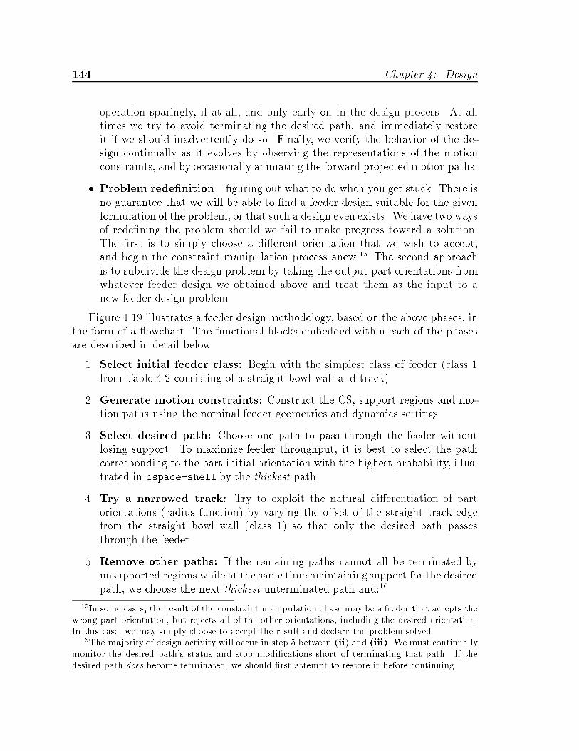
��� Chapter � Design
operation sparingly� if at all� and only early on in the design process� At alltimes we try to avoid terminating the desired path� and immediately restoreit if we should inadvertently do so� Finally� we verify the behavior of the de�sign continually as it evolves by observing the representations of the motionconstraints� and by occasionally animating the forward projected motion paths�
� Problem rede nition � �guring out what to do when you get stuck� There isno guarantee that we will be able to �nd a feeder design suitable for the givenformulation of the problem� or that such a design even exists� We have two waysof rede�ning the problem should we fail to make progress toward a solution�The �rst is to simply choose a di�erent orientation that we wish to accept�and begin the constraint manipulation process anew��� The second approachis to subdivide the design problem by taking the output part orientations fromwhatever feeder design we obtained above and treat them as the input to anew feeder design problem�
Figure ��� illustrates a feeder design methodology� based on the above phases� inthe form of a �owchart� The functional blocks embedded within each of the phasesare described in detail below�
�� Select initial feeder class� Begin with the simplest class of feeder �class �from Table �� consisting of a straight bowl wall and track��
�� Generate motion constraints� Construct the CS� support regions and mo�tion paths using the nominal feeder geometries and dynamics settings�
�� Select desired path� Choose one path to pass through the feeder withoutlosing support� To maximize feeder throughput� it is best to select the pathcorresponding to the part initial orientation with the highest probability� illus�trated in cspace�shell by the thickest path�
� Try a narrowed track� Try to exploit the natural di�erentiation of partorientations �radius function� by varying the o�set of the straight track edgefrom the straight bowl wall �class �� so that only the desired path passesthrough the feeder�
�� Remove other paths� If the remaining paths cannot all be terminated byunsupported regions while at the same timemaintaining support for the desiredpath� we choose the next thickest unterminated path and���
��In some cases the result of the constraint manipulation phase may be a feeder that accepts thewrong part orientation but rejects all of the other orientations including the desired orientation�In this case we may simply choose to accept the result and declare the problem solved�
��The majority of design activity will occur in step � between �ii� and �iii�� We must continuallymonitor the desired path�s status and stop modi�cations short of terminating that path� If thedesired path does become terminated we should �rst attempt to restore it before continuing�

�� The Design of Vibratory Bowl Feeders ���
(1) Select Initial Geometry
(2) Generate Motion Constraints
(3) Select Desired Path
(4) Try Narrowed Track
Remaining Paths Terminated?
(5) Select & Terminate Other Paths
(i) Generate Track Cutout
(ii) Redirect Paths
(iii) Modify Supports
(6) Keep Trying?
(7) Reconfigure Problem
(ii) CascadeFeatures
(i) Select NewDesired Path
Done!Y
N
Y
N
Formulate
Initial
Problem
Manipulate
Constraint
Representations
(Core Design Loop)
Redefine
Problem
Figure ���� Flowchart for a bowl feeder design strategy �see text��

��� Chapter � Design
i� Track cutout� Early on in the design process� we may try introducinga cutout near the unterminated path with the most di�erentiated valleyheight from the desired path� �If the unterminated path is higher in ythan the desired path �most likely case� then choose a left falling cutoutnear the unterminated path� Otherwise� choose a right or forward fallingpath near the unterminated path�� This corresponds to a class � feedergeometry from Table ���
ii� Redirect paths� Manipulate the CS surface to di�erentiate the unter�minated path from the desired path by creating or modifying a ridge orvalley on the CS �i�e� a bowl wall protrusion or cavity� features b� � c�from Table ���� This corresponds to a transition from a feeder class � �class � transition from Table ��� For non�class � bowl wall geometries�we may also vary the applied force vector to further di�erentiate pathsacross individual contact facets�
iii� Modify unsupported CS regions� To intercept the unterminated path�manipulate the support transition boundaries on the CS near a portion ofthe unterminated path on the CS ridge or valley feature� This correspondsto a transition from a feeder class � � class transition from Table ���
�� Repeat for other unterminated paths� Select other unterminated pathsand repeat step � until only the desired path passes through the feeder�
� Recon gure the design problem� If no progress is made after trying anumber of other paths���
i� Select another desired path� One option is to choose another path asthe desired path� Speci�cally� we choose the next thickest path as thedesired path and go back to step � In doing so� we are basically we�reaccepting a reduced feeder throughput����
� OR �
ii� Cascade lters� If some paths have been removed by the feeder featuresdesigned so far� we can locally decouple the problem by cascading feederfeatures� Speci�cally� we take the remaining paths from the existing setof feeder features and go back to step �� Essentially� we are designing anew feeder for the remaining paths inherited from the previous feeder inthe chain�
��The term a number is intentionally vague� Depending on the particular example the informa�tion provided by dynamic visualization of constraint coupling should quickly tell us whether or nota particular local manipulation strategy will pay o��
��Before doing this one might want to save the current feeder geometry and start out with newnominal bowl wall and track pro�les i�e� class � from Table ����
�� The Design of Vibratory Bowl Feeders ���
The traversal of the steps illustrated in the �owchart is carried out in three nestedloops� each of which deals more locally with a sub�problem of the design task and inmore detail than the enclosing loops� The three loops� each of which may be iteratedon a number of times in the course of a design� are given as�
� Feeder feature groupings � localization and cascading of feeder features�
� Selection of desired path � formulate the accept �i�e� passing� motiongoal so as to optimize the feeder throughput�
� Direct manipulation of motion constraints � modify the bowlwall and track polygons by manipulating the CS and support transi�tion boundaries� respectively� while focusing on each individual mo�tion path�
The innermost loop� forming the core of the design methodology � constraint visu�alization and manipulation � is embedded in the representations and design func�tions that form the cspace�shell environment� In Figure ��� this corresponds tosteps ��i�� �ii�� �iii� and step �� Surrounding this loop is the selection of the desiredaccept path corresponding to step �� in the initial problem formulation phase� andto step �i� in the problem rede�nition phase of design� Finally� the outermost loopinvolves selecting an initial �simple class �� feeder geometry that generates a seriesof motion paths for a given part geometry �step ��� During the problem rede�nitionphase this involves chaining the output of a partial feeder design into a subsequentfeeder design problem �step �ii���
���� Feeder Examples
Figure ���� is intended to serve as a roadmap for using the representations anddesign tools in cspace�shell more e�ectively by providing a consistent and orga�nized means of searching the space of designs for a solution while at the same timecontrolling the complexity inherent in the design process� For a given example� theintuition and experience gained by the designer might suggest alternative strategiesbased on the appearance of certain motion constraint features or constraint couplingcharacteristics observed during design� Indeed� the purpose of the representationsand interactive tools is to provide the necessary �exibility to the human designer todeal with individual cases in a correct and consistent manner� In the ideal case� the�right thing� to do during a given design session will become clear from the motionconstraint representations as the designer explores the design space�
Example �
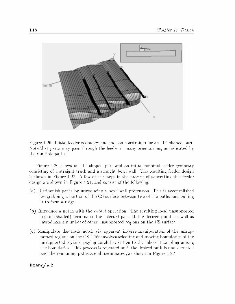
��� Chapter � Design
Figure ��� Initial feeder geometry and motion constraints for an �L��shaped part�Note that parts may pass through the feeder in many orientations� as indicated bythe multiple paths�
Figure �� shows an �L��shaped part and an initial nominal feeder geometryconsisting of a straight track and a straight bowl wall� The resulting feeder designis shown in Figure ���� A few of the steps in the process of generating this feederdesign are shown in Figure ���� and consist of the following�
a� Distinguish paths by introducing a bowl wall protrusion� This is accomplishedby grabbing a portion of the CS surface between two of the paths and pullingit to form a ridge�
b� Introduce a notch with the cutout operation� The resulting local unsupportedregion �shaded� terminates the selected path at the desired point� as well asintroduces a number of other unsupported regions on the CS surface�
c� Manipulate the track notch via apparent inverse manipulation of the unsup�ported regions on the CS� This involves selecting and moving boundaries of theunsupported regions� paying careful attention to the inherent coupling amongthe boundaries� This process is repeated until the desired path is unobstructedand the remaining paths are all terminated� as shown in Figure ����
Example �
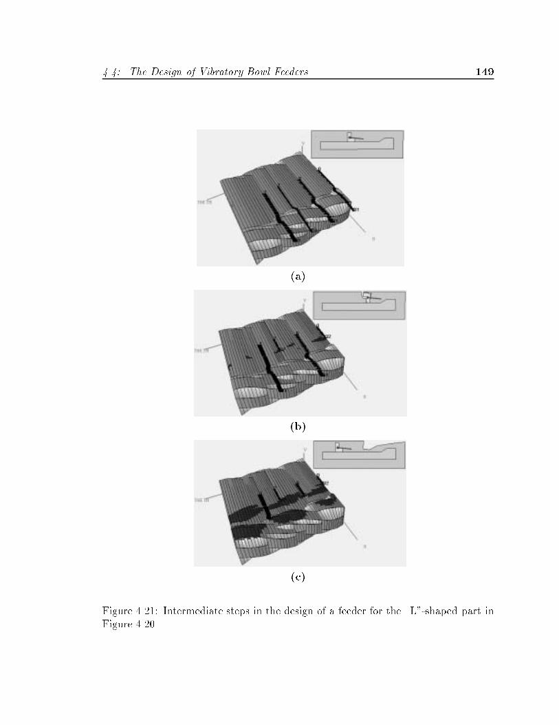
�� The Design of Vibratory Bowl Feeders ���
a�
b�
c�
Figure ���� Intermediate steps in the design of a feeder for the �L��shaped part inFigure ���
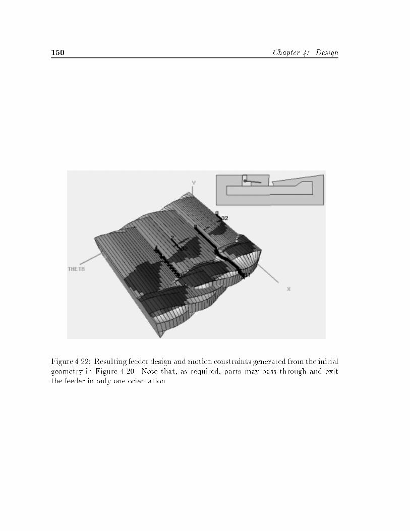
�� Chapter � Design
Figure ���� Resulting feeder design and motion constraints generated from the initialgeometry in Figure ��� Note that� as required� parts may pass through and exitthe feeder in only one orientation�
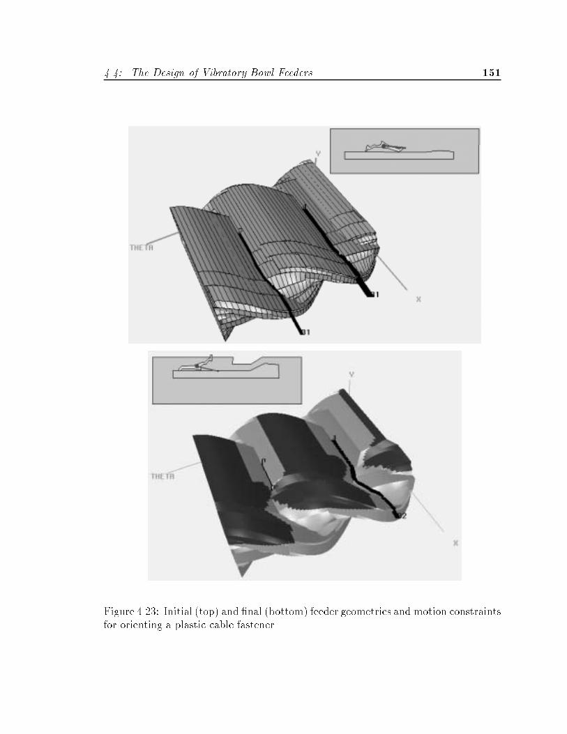
�� The Design of Vibratory Bowl Feeders ���
Figure ���� Initial �top� and �nal �bottom� feeder geometries and motion constraintsfor orienting a plastic cable fastener�

��� Chapter � Design
The initial feeder geometry and motion constraints for a part consisting of aplastic cable fastener is shown in the top of Figure ���� As in the previous ex�ample� a protrusion in the bowl wall was introduced by �pulling� on the surface ofthe CS to form a ridge in order to help distinguish among the two motion paths�both of which initially travel nearly parallel to one another across the CS in the� direction� The track contour was developed by initially pulling a pair of pointson the track boundary toward the bowl wall to produce unsupported regions on theCS� The unsupported regions were then manipulated within the motion constraintrepresentation via apparent inversion� After a few iterations the motion constraintscharacteristic of a motion �lter were obtained� as shown in the bottom of Figure ����together with the corresponding bowl wall and track geometries�
Example �
The top of Figure �� shows the initial feeder geometry for an x�acto razorblade� Here� as in the previous examples� a protrusion has been introduced intothe wall pro�le to form a ridge on the CS� Unlike the previous examples� however�the purpose of this ridge is to catch and reorient those parts that are sliding withtheir major axis perpendicular to the wall� On the CS� the ridges forming thesereorienting constraints may be characterized as fences that are angled relative tothe � direction� thus diverting or guiding multiple motion paths toward a subsetof common orientations �� positions��� The rather oddly shaped gap in the trackshown in the bottom of Figure �� was introduced using the cutout operator to �lterout the undesirable motion paths� The track contour produced by the cutout in thiscase required only minor modi�cation to produce the �nal feeder geometry shown�
����� Physical Experiments
Models for selected part� bowl wall and support track pro�les were constructedfrom plexiglass and tested by placing the parts on the track surface in random initialorientations and allowing them to slide downhill while applying a slight verticalvibration to the track surface�� Figure ��� shows the hardware used to test someof the feeder designs developed using cspace�shell�
The part motions� and resulting feeder behavior� closely followed the motion pathspredicted by cspace�shell� Photographs of one of the experiments run for the partand feeder in Figure ��� �top� are shown in Figure ��� and Figure �� �
�As noted earlier the ability to reorient rather than reject some part orientations has the ad�vantage of increasing the throughput of the resulting feeder�
�Since the amplitude of vibration applied to the track was insu�cient to cause the parts to�hop� the track was tilted downward so that gravity would drive the part motion�

�� The Design of Vibratory Bowl Feeders ���
Figure ��� Initial �top� and �nal �bottom� feeder geometries and motion constraintsfor orienting x�acto razor blades�

��� Chapter � Design
Figure ���� Hardware for testing feeder designs consisting of a plexiglass wall andtrack mounted on a tilted shaker table �top�� and a closeup of the shaker assembly�bottom��
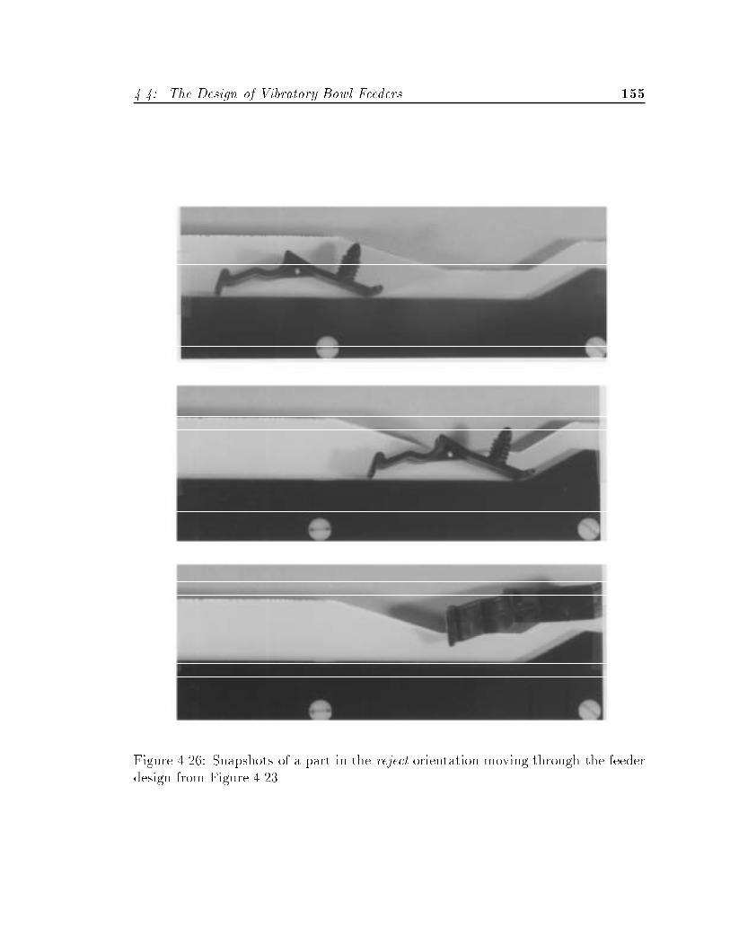
�� The Design of Vibratory Bowl Feeders ���
Figure ���� Snapshots of a part in the reject orientation moving through the feederdesign from Figure ����
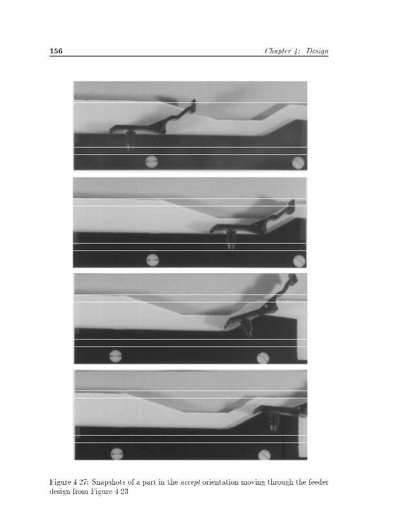
��� Chapter � Design
Figure �� � Snapshots of a part in the accept orientation moving through the feederdesign from Figure ����

�� The Design of Compliant Assemblies ���
��� The Design of Compliant Assemblies
To further demonstrate the applicability of the representation and manipulation toolsdeveloped earlier in this chapter� we will now turn our attention from vibratory bowlfeeders to the design and analysis of compliant assemblies introduced in Section ����In particular� we shall illustrate the �exibility of the analysis and design tools devel�oped in cspace�shell by adapting them for use in the domain of assembly�
����� Non�assembly Constraints
The feeders designed earlier have only one functional requirement � orienting parts�Whatever functional requirements that the speci�c part geometries themselves wererequired to meet were not considered directly as they were� in a sense� orthogonalto the function of the feeder� In our examples� whatever external constraints on thepart geometries that might have existed were implicitly satis�ed by the assumptionthat� in general� the part geometries themselves would not be modi�ed during feederdesign��� In the case of assembly� however� both interacting parts typically haveto satisfy a number of constraints that may have nothing to do with the assemblyprocess� Examples of some non�assembly constraints include� maintaining a mini�mum area if contact between bearing surfaces that must be aligned and unobstructed�e�g� shaft and bearing represented as a peg�in�hole�� minimum area contact surfacesfor electrical connectors� reference surfaces that must remain exposed to subsequentsubassemblies or grippers� part features and dimensions required for strength andsti�ness� and features necessary for locating and machining the parts before assem�bly�
One approach to preserving non�assembly constraints is to simply lock certainobject features �both peg and hole� into relative con�gurations at the goal state thatensure the necessary local constraints are maintained� This is equivalent to dividingthe set of edges and vertices describing each part into two classes� mutable and �xed�Modi�cations to mutable geometric and dynamics parameters that allow these keyfeature pairs to be brought into contact at the goal state of an assembly operationwould also� presumably� satisfy both the assembly and non�assembly constraint sets�The advantage of this approach is that non�assembly constraints may be expressedsimply as additional constraints on the existing set of design parameters� no matterwhat their origin� The disadvantage to simply �xing existing parameters is that�since we do not know the origin of the constraints� we have no �exibility in terms ofoptimizing them together with motion constraints for assembly�
In the following examples we will follow the above approach� For the sake of
��For those examples where we did modify the part design we assumed that the designer keptthese constraints in mind during the design process so that any modi�cations would not compromisepart functionality�
��� Chapter � Design
generality it would be desirable to combine the representations for non�assemblyconstraints with the motion constraint representations in con�guration space wher�ever possible� Such representations would be particularly useful in the e�ort todesign components and subassemblies concurrently in the context of both productand process constraints� Given the wide range of such outside constraints� however�it is likely that di�erent representation combinations would have to be developed fordi�erent classes of assemblies� These issues remain an open area for future research�
����� Methodology
In terms of managing the complexity due to coupling among motion constraint repre�sentations� the design methodology for compliant assemblies is considerably simplerthan that necessary for vibratory bowl feeders� In particular� since we will focus ourattention on the local region surrounding the hole on the CS� as described in Sec�tion ���� we need not be concerned with the introduction of undesirable constraintfeatures elsewhere on the surface of the CS��� In addition� since we do not considerout�of�plane part motions in assembly� we may avoid the very non�linear couplingobserved between shape modi�cations and the support transition boundaries� Whatremains from cspace�shell as developed for bowl feeder design are the kinematicconstraints of the CS surface and the forward projections expressed as discrete mo�tion paths� With respect to the feeder design methodology �owchart of Figure ����we may concern ourselves with only step ��ii� Redirect Paths of the innermostloop���
Interactive design of motion constraints for assembly consists of modifying themutable subsets of both part geometries via apparent inversion of contact facetson the CS surface� varying the reference point of the moving part �i�e� compliancecenter� directly� and varying the dynamics parameters� We will assume a generalizeddamper model of compliance mapping di�erences in velocity between the assemblyrobot and the part into forces on the part �see Section ����� Under this model� theforce vector applied through the moving part�s reference point in cspace�shell isinterpreted as a commanded velocity from the assembly robot� As for bowl feeders�the dynamics of part motion is assumed to be quasi�static �see Section ������ For thiscase� the dynamics parameters consist of the direction of the force�velocity vectorapplied to the compliance center� which is assumed to be parallel to the intendednominal assembly path� and the coe�cient of friction ��
Since� for the purposes of expediency� we are borrowing design tools originallydesigned for the design of bowl feeders� a few design operations must be carried out
��We should keep in mind however that proximity of motion constraint surfaces in con�gurationspace does not necessarily require proximity of geometric features on an object�
��The rest of the feeder design methodology is unnecessary for assembly as it is dedicated todealing with coupling and managing interactions among global constraints�

�� The Design of Compliant Assemblies ���
somewhat indirectly� Changes to the rotational compliance C�� relative to the trans�lational compliance terms� may be carried out by varying the normalized e�ectiveinertia of the of moving object in the form of the radius of gyration by meansof a slider� At present� the apparent inversion tools do not support the manipu�lation of the moving object�s reference point via changes to the motion constraintrepresentations���
The initial position from which each motion path starts� consisting of a �x� y� ��point in the free region of con�guration space� is chosen manually via sliders� Weexplore the behavior of the assembly over a range of parameters possible underpositional and control uncertainty by selecting discrete values of the initial positionand dynamics parameters� as noted in Section ���� The resulting bundles of discretepaths sample the full forward projection of motion for the assembly task underuncertainty�
����� Assembly Examples
Example �
Figure ��� shows the change in motion constraints resulting from the additionof chamfers to both a peg and hole� The constraints shown form the entry region tothe hole surrounding the goal region of the assembly �i�e� the peg positioned insidethe hole�� The chamfers in this example were generated directly from the geometryof the parts� with the motion constraint representation serving only to con�rm thatthe desired functional characteristics had been achieved�
Example �
Figure ��� illustrates another aspect of the design of compliant assemblies�Speci�cally� the location of the center of compliance relative to the tip of the pegdetermines whether or not the motion constraint boundaries surrounding the goalregion of the assembly guide motions to the goal in the presence of rotational mis�alignments �i�e� o�sets in the � direction�� as shown in the bottom of Figure ����The cup�like curvature of the motion constraint boundaries in the ��direction maybe viewed as a form of rotational chamfer� whose function is analogous to that ofthe chamfers introduced to the part geometries in the previous example� Thus� themotion constraint representation serves to illustrate the similar e�ects achieved byproper placement of the compliant center �assembly strategy� and the addition ofchamfers �part geometry� on the success or failure of an assembly task�
��It is possible to indirectly modify the reference point from the motion constraints by selectingall vertices of the moving polygon from the CS� Uniformmodi�cations to these vertices has a similare�ect but in the opposite xy direction� to modifying the reference point alone�
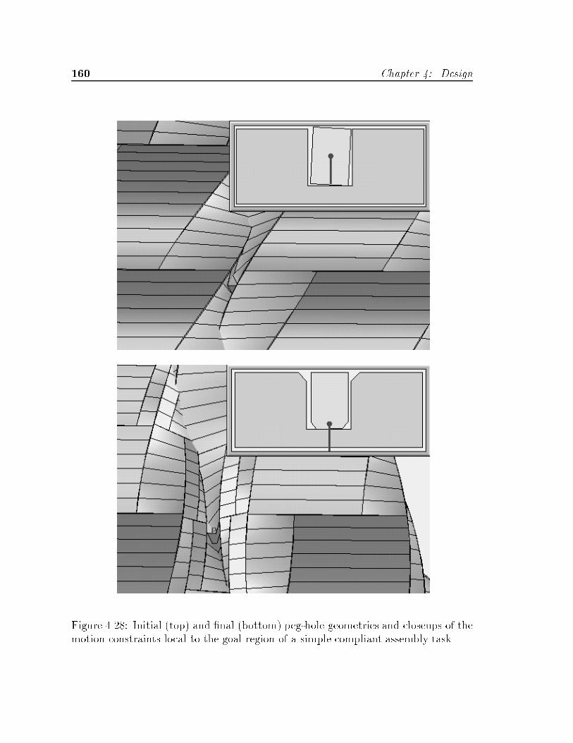
�� Chapter � Design
Figure ���� Initial �top� and �nal �bottom� peg�hole geometries and closeups of themotion constraints local to the goal region of a simple compliant assembly task�

�� The Design of Compliant Assemblies ���
Figure ���� The e�ect of moving the compliant center along a peg�s major axis fromthe middle of the peg �top� to the tip of the peg �bottom�� on the rotational aspectsof the motion constraints �� dimension of the con�guration space��

��� Chapter � Design
Example �
Figure �� shows a somewhat more complex pair of part geometries compris�ing an electrical plug connector� Unlike the peg and hole example in Figure ����modi�cations to the part geometries were made entirely from within the motion con�straint representation using apparent inversion� Speci�cally� constraint surfaces nearthe goal region in Figure �� �top� caused the assembly to jam in the presence ofrotational misalignments� To modify the design� the constraint surfaces in questionwere selected and pushed out of the way in order to widen the access to the goalregion� with the corresponding part geometries being modi�ed accordingly by meansof apparent inversion� It is interesting to note that geometric modi�cations in thisexample were made to a number of part features �i�e� the entry guides and center pinof the socket� that are not proximal on the part contour but nevertheless produceproximal �intersecting� motion constraint surfaces in con�guration space�
��� Discussion
We will brie�y discuss some of the observations made after using the representationsand tools for design� We will also consider some of the limitations of and suggestpossible extensions to the implementation of cspace�shell�
How useful were the representations and tools for design� As expected� the spaceof design parameters was very large even for relatively simple systems� Given this�the following general conclusions about the use of motion constraint representationsfor design were rea�rmed�
� The ability to visualize the coupling between parameters and constraints� aswell as the sensitivity of a system to local design changes� was crucial in suc�cessfully iterating toward a design goal for highly coupled systems like bowlfeeders�
� The manipulation of design parameters directly in the context of the motionconstraint representations provided a good idea of which way to go �locally�to reach a desired design state� although non�linear coupling often made accu�rately predicting the e�ects of large excursions in design space di�cult�
� Classi�cations and taxonomies of shapes were somewhat useful for starting outa design iteration loop by quickly getting to a region of design space� However�the parametric �tweaking� that takes place afterward was a necessary and sig�ni�cant component of achieving a successful design� Basically� taxonomies andshape classi�cations can sometimes get one close to a good design� but almostinvariable detailed design is necessary to make things work for a particularexample�
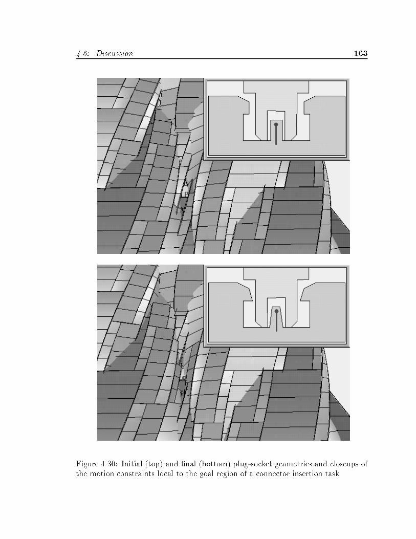
� � Discussion ���
Figure ��� Initial �top� and �nal �bottom� plug�socket geometries and closeups ofthe motion constraints local to the goal region of a connector insertion task�

��� Chapter � Design
How e�ective and easy to use were the design functions� The in�exibility resultingfrom a number of the approximations and additional constraints imposed for thepurposes of easier implementation of cspace�shell proved to be somewhat more ofa nuisance than anticipated�
� Generally speaking� the design functions allowed us to reach desired points indesign space % eventually�
� For bowl feeder design� having to jump back and forth between modi�cations tothe kinematic constraints of the CS and the support constraints of the supporttransition boundaries within the innermost design loop of the methodology inFigure ��� was awkward� In particular� much of the coupling between con�straints at this stage appeared to be due to the fact that we were representingthe support transition boundaries as the intersection of the supported regionof con�guration space with the kinematic constraints of the CS surface �seeSection ����� Although prudent in terms of implementation complexity� theresulting coupling and lack of information regarding support of con�gurationsnot on the CS surface were a nuisance� Ideally� we would have liked to be ableto manipulate both the CS surface and the surface of the supported region� asillustrated in Figure ����� in the full �x� y� �� con�guration space independentlyof one another�
� The requirement that modi�cations via apparent inversion to the CS facetsand support transition boundaries could only be made in an �x� y� plane incon�guration space was restrictive� Again� prudence in the implementationplaced additional constraints on the �exibility of the tools� Ideally� since wevisualize the motion constraints in the full �x� y� �� con�guration space� wewould also like to be able to manipulate these constraints fully in the samespace�
� With our motion constraint representations we have moved beyond modelingobject geometry to make explicit and accessible the motion constraints implicitin the interaction of objects� Recalling Figure �� we note that the ultimateobjective of the design exercise is to produce desired object motions� In a sense�the motion constraints are secondary to the paths themselves� Ideally� we wouldlike to be able to manipulate the motion paths more directly via apparentinversion to achieve a design� instead of doing so indirectly by manipulatingconstraints on the motions�
Finally� some general observations about the design of motion constraints gainedfrom the above examples�

��� Summary ���
� Global coupling between design parameters and motion constraints is whatmakes geometric design di�cult� Unlike application domains that may be de�coupled into lumped parameter elements� such as electrical circuits or hydraulicnetworks� geometric interactions between objects are inherently coupled� Anysystem that attempts to model such systems accurately must capture this cou�pling�
� The e�ects of coupling were particularly apparent in the bowl feeder examples�Since vibratory feeders are sensorless� they can neither predict nor observe theorientation of the next part to enter the feeder� Therefore� since part�feederinteractions cannot be made to occur selectively� the designer must take intoconsideration the motion constraints produced by interactions along all possiblemotion paths� Everything that can happen will happen�
� In general� design for compliant assembly seems to be easier because we needfocus on only a very local set of constraints� This conclusion may be somewhatmisleading� however� since we have ignored a signi�cant aspect of assemblydesign � getting a set of assembly motion constraints that are consistent withwhatever other external constraints may be imposed on a part�s design�
�� Summary
In this chapter we have taken the motion constraint representations developed inChapter � and extended them in a number of ways to address the issue of design�We examined some of the di�culties of generating consistent shapes from a priorispeci�cations of function in terms of motion constraints� and in particular we illus�trated how the notion of generating functional shapes by sweeping �xed shapes alongspeci�ed motion paths does not guarantee that the desired motion constraints willbe achieved� We introduced the space of design parameters as a domain in whichdesign of shape and other parameters could viewed in the context of a search� Wedeveloped a set of design functions to operate on design parameters that were di�vided into two classes� parametric functions� which we labeled apparent inversion�that allow us to select and consistently manipulate design parameters indirectly inthe context of motion constraints� and topological functions� one example of which isan imposed out�of�plane swept motion designed to cut out contours in a supportingtrack�
We introduced and explored the notion of dynamic constraint visualization wheremanipulation of constraints and parameters� �i� allow us to explore the neighborhoodof a point in design space and identify what changes to a design are likely to achievea desired function� and �ii� keep us aware of what is and is not possible to modifyindependently� In particular� we noted that coupling between di�erent constraint

��� Chapter � Design
representations and the underlying design parameters posed a serious challenge tothe design of interacting shapes�
We presented an overview of an implemented design and analysis toolkit � cspace�shell� that provides a computational environment to support the representation and in�teractive manipulation of motion constraints for design� We gave an overview ofa design methodology for using this toolkit in the design of vibratory bowl feedersand compliant peg�in�hole assemblies� In developing this methodology we also in�troduced a number of constructs designed to organize our search of a large designspace and help control the level of complexity and coupling between parameters andconstraint representations� Finally� we presented a series of design examples for bowlfeeders and� to a more limited extent� peg�in�hole assemblies in which we utilized andevaluated the toolkit�

Implementation
Chapter �
��� Goals
The primary motivation for implementing the motion constraint based shape de�sign system was to provide both a research tool and proof of concept demonstrationfor visualizing and designing function from shape� The following goals guided themultitude of choices� assumptions� and optimizations that form the resulting imple�mentation�
� SPEED � Compute and recompute the set of motion constraints from shapeat speeds that are su�cient for near real�time interactive feedback�
� Emphasis on the modi�cation of shape parameters for the purposes of design�This is in contrast to existing con�guration space based analysis and planningsystems that emphasize the computation of motions with respect to staticmotion constraints derived from �xed shapes�
� Provide direct access to design parameters from within the same functionalrepresentations that are used for visualization and analysis� This includesproviding as natural and intuitive an interface as possible for the manipulationof representations design parameters by means of apparent�inversionfunctions mapping interactive user inputs in con�guration space to shape�
In addition to these general goals� the implementation has been tailored for rep�resenting and manipulating motion constraints that are particularly well suited fordesign in the domain of vibratory part feeders� although additional features havebeen added for modeling and design of compliant assembly tasks�
��
��� Chapter � Implementation
��� System Overview
The interactive shape design system consists of approximately ��� lines of C sourcecode compiled to run on a Silicon Graphics Personal Iris workstation� The code isorganized into the following major modules�
cspace�shell Core routines including the interactive graphical user interface andmain loop running the con�guration space display for representing and manip�ulating motion constraints and shape�
cs routines Routines to generate CS facets�
cs motions Routines for the incremental computation of motion paths and local CStopology�
cs support Routines to compute the approximate boundaries of supported and un�supported regions on CS facets� and generating track cutouts for imposed partmotions�
cs selection Routines that allow the user to select and modify part� bowl andtrack vertices via changes to the CS or LOS boundaries�
The interactions among the major modules is illustrated in Figure ���� A num�ber of additional �les provide data structure de�nitions� I�O support and variousutilities�� The remainder of this chapter presents in detail the implementation of themajor components of cspace�shell and its subroutines�
The main event loop in cspace�shell handles all of the functions for displayingobjects and their motion constraints in con�guration space� User selection of orincrementalmodi�cations to any of the shape parameters automatically cause the CSto be continuously recomputed and displayed during the modi�cation� If enabled� thesupport regions on each of the facets in the CS are also recomputed and displayed�Other functions that need not or cannot be performed continuously� such as theintegration or animation of motion paths� are executed once �on demand� by theuser��
�These �les include� cs data structures�h cs file io cs to iris cslice iriscs utilities and cs iris utilities�
�Numerical integration of motion paths is the most computationally expensive operation per�formed in cspace�shell and would be unable to provide acceptably fast feedback to the userduring a design operation�

��� System Overview ���
CSpace-ShellGraphicalUser Interface
CS_Routines CS_MotionsCS_Support
Computeand RenderCS Facets
ComputeLocal CS Topology,
Compute andRender Motion
Paths
Computeand Render
Facet SupportMaps
Various Utility Modules
Figure ���� General overview of the major modules comprising the interactive motionconstraint design system�

�� Chapter � Implementation
��� Generating Kinematic Constraints
����� Contact Facets
We explicitly model the two basic types of single�contact interactions between a pairof planar polygons as constraint facets�
� type A � an edge of Polygon A �moving� touching a vertex of Polygon B�stationary�� and
� type B � an edge of Polygon B touching a vertex of Polygon A�
The contact generating each facet type reduces the degrees of freedom of the movingpolygon from three to two� A convenient parameterization for the remaining twodegrees of freedom is p and � as shown in Figure ���� The p parameter determinesthe non�dimensional position �� �� along a polygon�s edge at which a vertex of theother polygon contacts that edge� The � parameter is the orientation of the movingpolygon� and is the same � used in the �x� y� �� con�guration space� The values of pand � thus determine the position of a point on the surface of a facet that is itselfembedded in the �x� y� �� con�guration space�
Using the parameters �p� �� we may write the equations for a point on a facetsurface� For a type A facet� we have�
FA�p� �� " RBj �Rot����RA
i � p EAi � �����
p � �� �� �����
� � ��min� �max� �����
where RBj is the position vector of the jth vertex of the stationary polygon from
the origin of the world coordinates� RAi and EA
i are the position and edge vectors�respectively� of the ith vertex and edge of the moving polygon with respect to thatpolygon�s reference point� and p and � are the facet parameters� Rot��� is therotational transform�
Rot��� "
�cos � � sin �sin � cos �
�
Similarly� for a type B facet we have�
FB�p� �� " RBj � p EB
j �Rot����RAi � ����
p � �� �� �����
� "� ��min� �max� �����

��� Generating Kinematic Constraints ���
X
Y
X
Y
θ
X
Y
θ
X
Y
pθ
p
θ
p
θ
p
θ
Figure ���� Parameterization of facets by p and ��
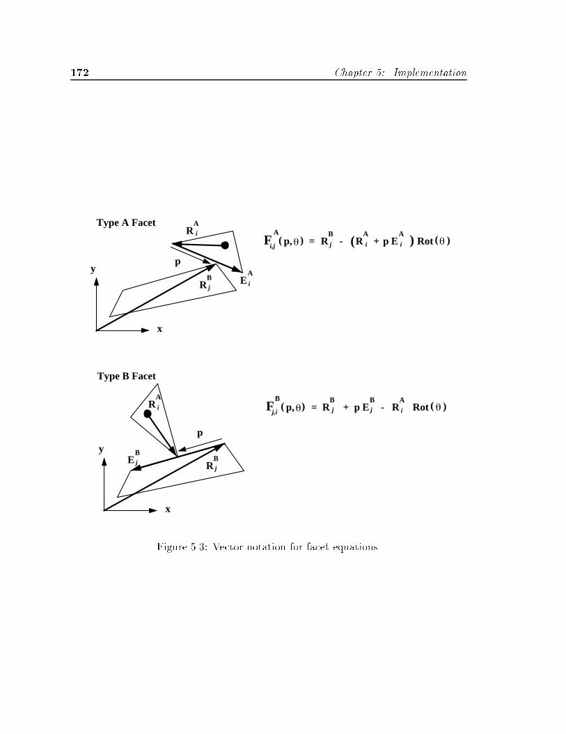
��� Chapter � Implementation
Type A Facet
Type B Facet
θF p,( )i,j
A= θRot ( )R
Ai E
Aip+( )R
Bj -
θp,( )Fj,i
B= θRot ( )R
AiE
Bjp -R
Bj +
p
x
yE
Ai
RAi
RBj
p
x
y
RAi
EBj R
Bj
Figure ���� Vector notation for facet equations�
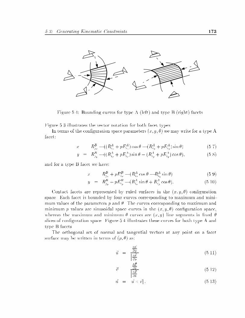
��� Generating Kinematic Constraints ���
Figure ��� Bounding curves for type A �left� and type B �right� facets�
Figure ��� illustrates the vector notation for both facet types�In terms of the con�guration space parameters �x� y� �� we may write for a type A
facet�
x " RBjx � ��RA
ix � pEAix� cos � � �RA
iy � pEAiy� sin �� ��� �
y " RBjy � ��RA
ix � pEAix� sin � � �RA
iy � pEAiy� cos ��� �����
and for a type B facet we have�
x " RBjx � pEB
ix � �RAix cos � �RA
iy sin �� �����
y " RBjy � pEB
iy � �RAix sin � �RA
iy cos ��� �����
Contact facets are represented by ruled surfaces in the �x� y� �� con�gurationspace� Each facet is bounded by four curves corresponding to maximum and mini�mum values of the parameters p and �� The curves corresponding to maximum andminimum p values are sinusoidal space curves in the �x� y� �� con�guration space�whereas the maximum and minimum � curves are �x� y� line segments in �xed �slices of con�guration space� Figure �� illustrates these curves for both type A andtype B facets�
The orthogonal set of normal and tangential vectors at any point on a facetsurface may be written in terms of �p� �� as�
u "� �F�p� �F�p
������
v "� �F��� �F��
������
n " ju� vj � ������
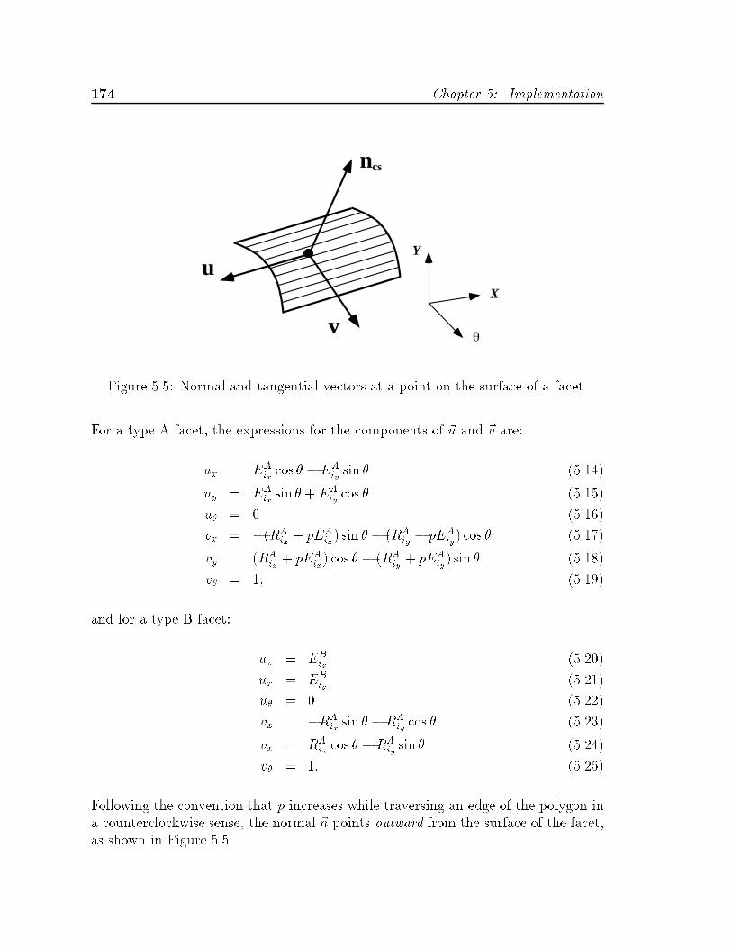
��� Chapter � Implementation
θ
X
Y
ncs
u
v
Figure ���� Normal and tangential vectors at a point on the surface of a facet�
For a type A facet� the expressions for the components of u and v are�
ux " EAix cos � �EA
iy sin � �����
uy " EAix sin � � EA
iy cos � ������
u� " ������
vx " ��RAix� pEA
ix� sin � � �RA
iy� pEA
iy� cos � ���� �
vy " �RAix� pEA
ix� cos � � �RA
iy� pEA
iy� sin � ������
v� " �� ������
and for a type B facet�
ux " EBix �����
ux " EBiy ������
u� " ������
vx " �RAix sin � �RA
iy cos � ������
vx " RAix cos � �RA
iy sin � �����
v� " �� ������
Following the convention that p increases while traversing an edge of the polygon ina counterclockwise sense� the normal n points outward from the surface of the facet�as shown in Figure ����
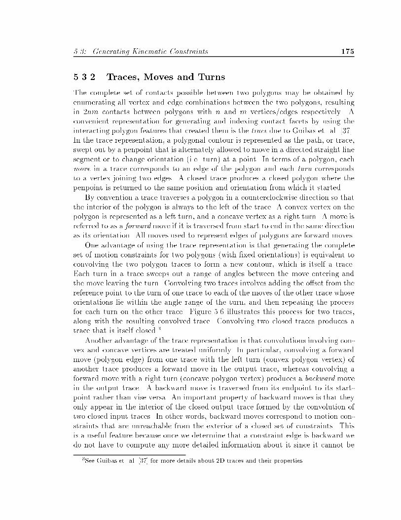
��� Generating Kinematic Constraints ���
����� Traces� Moves and Turns
The complete set of contacts possible between two polygons may be obtained byenumerating all vertex and edge combinations between the two polygons� resultingin �nm contacts between polygons with n and m vertices�edges respectively� Aconvenient representation for generating and indexing contact facets by using theinteracting polygon features that created them is the trace due to Guibas et� al� �� ��In the trace representation� a polygonal contour is represented as the path� or trace�swept out by a penpoint that is alternately allowed to move in a directed straight linesegment or to change orientation �i�e� turn� at a point� In terms of a polygon� eachmove in a trace corresponds to an edge of the polygon and each turn correspondsto a vertex joining two edges� A closed trace produces a closed polygon where thepenpoint is returned to the same position and orientation from which it started�
By convention a trace traverses a polygon in a counterclockwise direction so thatthe interior of the polygon is always to the left of the trace� A convex vertex on thepolygon is represented as a left turn� and a concave vertex as a right turn� A move isreferred to as a forwardmove if it is traversed from start to end in the same directionas its orientation� All moves used to represent edges of polygons are forward moves�
One advantage of using the trace representation is that generating the completeset of motion constraints for two polygons �with �xed orientations� is equivalent toconvolving the two polygon traces to form a new contour� which is itself a trace�Each turn in a trace sweeps out a range of angles between the move entering andthe move leaving the turn� Convolving two traces involves adding the o�set from thereference point to the turn of one trace to each of the moves of the other trace whoseorientations lie within the angle range of the turn� and then repeating the processfor each turn on the other trace� Figure ��� illustrates this process for two traces�along with the resulting convolved trace� Convolving two closed traces produces atrace that is itself closed��
Another advantage of the trace representation is that convolutions involving con�vex and concave vertices are treated uniformly� In particular� convolving a forwardmove �polygon edge� from one trace with the left turn �convex polygon vertex� ofanother trace produces a forward move in the output trace� whereas convolving aforward move with a right turn �concave polygon vertex� produces a backward movein the output trace� A backward move is traversed from its endpoint to its start�point rather than vise versa� An important property of backward moves is that theyonly appear in the interior of the closed output trace formed by the convolution oftwo closed input traces� In other words� backward moves correspond to motion con�straints that are unreachable from the exterior of a closed set of constraints� Thisis a useful feature because once we determine that a constraint edge is backward wedo not have to compute any more detailed information about it since it cannot be
�See Guibas et� al� ���� for more details about �D traces and their properties�

��� Chapter � Implementation
*
A B CS
Figure ���� Planar polygons represented as traces� and the trace corresponding totheir convolution�
on the surface of the CS��
When one of the planar polygons is allowed to rotate� as is the case in cspace�shell�we use a generalization of the trace representation in which each of the facets de�scribed earlier corresponds to a move of the convolved trace that is swept in the �dimension of the �x� y� �� con�guration space over the entire angle range for whichthat move is valid� Speci�cally� a facet is a move �edge� of one polygon that is o�setby the position of a turn �vertex� of the other polygon over the entire range of anglesfor which the move�s orientation lies within the turn�s angle range� Using the tracenotation� a facet is identi�ed by a type �type A or type B�� an index to a trace move�and an index to a trace turn� This type�move�turn indexing scheme is particularlyuseful in determining the topological relationships between facets forming the CSin con�guration space� Equations for a facet expressed as turns and moves can bederived from equations ��� and �� by substituting a turn for the R
A�Bi and a move
for EA�Bi ��
Enumerating and computing the complete set of individual constraint facets fortwo interacting polygons involves a relatively small amount of computation# theoverall complexity� both in size and time� is O�n�� where n is the typical number ofedges�vertices in each of the polygons� Computing the intersections and topological
�We will still enumerate facets corresponding to backward moves in our CS data structurebecause they provide topological closure of the set of facet in con�guration space and are useful indetermining facet adjacency�
�In cspace�shell the moving polygon is re�ected through the origin before being converted toa trace so the ��� sign in equations ��� and ��� would be replaced with a ��� sign�

�� Computing Motions ���
relationships between all facets in the CS� however� is generally a more di�cult andcomputationally expensive proposition�� Fortunately� for the purpose of representingthe CS graphically it is su�cient to compute only the complete set of individualfacets� For the purpose of computing object motions� however� we will need tocompute at least those topological features on the CS that constrain speci�c motions�In the next section we will describe these computations in more detail along withthe procedures for computing speci�c object motions�
In summary� the CS is constructed as an array of individual facets representingcontacts between edge and vertex feature pairs of two polygons� There is no explicitrepresentation of the relationships between the facets in the CS for the purposes ofrendering� This is done in order to enhance the speed at which CS surfaces may begenerated� rendered and manipulated� Speci�cally� by utilizing the depth bu�er� ofthe Iris workstation to hide those portions of the facets that are occluded by otherfacets� we are be able to generate and render a detailed graphical image of the CS innear real�time� as is necessary for implementing the kind of interactive manipulationfeatures discussed in earlier chapters�
��� Computing Motions
Part motions are represented as paths in con�guration space� approximated at thelowest level by a set of discrete points� Speci�cally� a motion path is represented incspace�shell as an array of contact states� where each contact state contains anarray of those points along a path that are in contact with the same set of facets�Speci�cally� a contact state encapsulates that portion of a path that is in contactwith the same set of facets corresponding to contacts between topologically distinctpairs of features of the moving and stationary objects� A contact state may containa point or set of points in contact with a single facet� an edge between two facets�a vertex formed by three facets� or no facets at all �i�e� a free or unconstrainedmotion���
The task of computing paths in cspace�shell is divided into two distinct pro�cesses� determining the local topology of the CS and piecewise numerical integration
�The worst case complexity is On����The depth bu�er or Z�bu�er is a relatively standard piece of graphics hardware in which
the distance from the viewing plane to each point of a rendered object is computed and used todetermine whether or that point should be drawn� A point on an object being drawn such as acontact facet that is further away from the viewing plane than a previously drawn point with thesame x� y� screen position will not be drawn� In this way overlapping or occluded objects aredrawn correctly and quickly�
�In those cases where due to a geometric coincidence more than three facets can come intocontact at a point the extraneous are removed from the contact state� See the description ofdetect new contacts�� in Section ��������
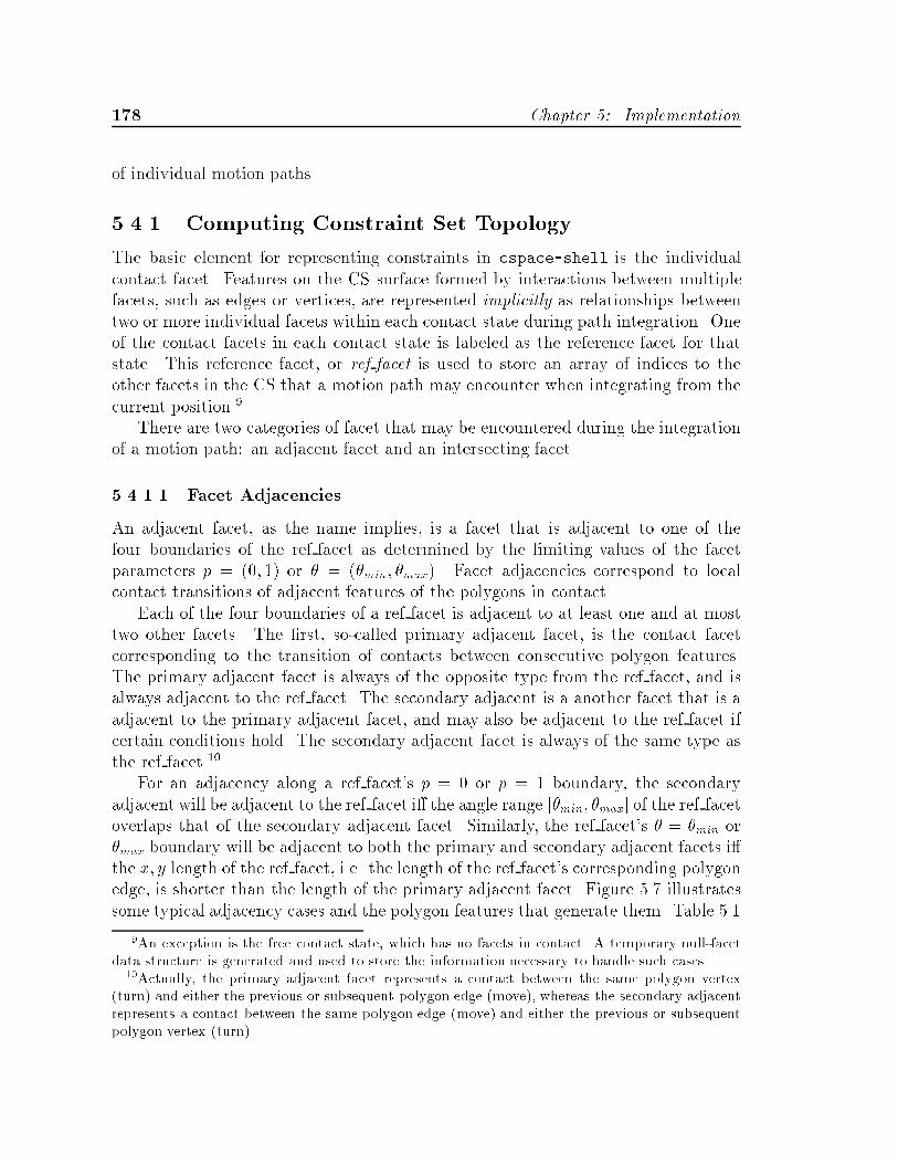
��� Chapter � Implementation
of individual motion paths�
����� Computing Constraint Set Topology
The basic element for representing constraints in cspace�shell is the individualcontact facet� Features on the CS surface formed by interactions between multiplefacets� such as edges or vertices� are represented implicitly as relationships betweentwo or more individual facets within each contact state during path integration� Oneof the contact facets in each contact state is labeled as the reference facet for thatstate� This reference facet� or ref facet is used to store an array of indices to theother facets in the CS that a motion path may encounter when integrating from thecurrent position�
There are two categories of facet that may be encountered during the integrationof a motion path� an adjacent facet and an intersecting facet�
������� Facet Adjacencies
An adjacent facet� as the name implies� is a facet that is adjacent to one of thefour boundaries of the ref facet as determined by the limiting values of the facetparameters p " �� �� or � " ��min� �max�� Facet adjacencies correspond to localcontact transitions of adjacent features of the polygons in contact�
Each of the four boundaries of a ref facet is adjacent to at least one and at mosttwo other facets� The �rst� so�called primary adjacent facet� is the contact facetcorresponding to the transition of contacts between consecutive polygon features�The primary adjacent facet is always of the opposite type from the ref facet� and isalways adjacent to the ref facet� The secondary adjacent is a another facet that is aadjacent to the primary adjacent facet� and may also be adjacent to the ref facet ifcertain conditions hold� The secondary adjacent facet is always of the same type asthe ref facet��
For an adjacency along a ref facet�s p " or p " � boundary� the secondaryadjacent will be adjacent to the ref facet i� the angle range ��min� �max� of the ref facetoverlaps that of the secondary adjacent facet� Similarly� the ref facet�s � " �min or�max boundary will be adjacent to both the primary and secondary adjacent facets i�the x� y length of the ref facet� i�e� the length of the ref facet�s corresponding polygonedge� is shorter than the length of the primary adjacent facet� Figure �� illustratessome typical adjacency cases and the polygon features that generate them� Table ���
An exception is the free contact state which has no facets in contact� A temporary null�facetdata structure is generated and used to store the information necessary to handle such cases�
�Actually the primary adjacent facet represents a contact between the same polygon vertexturn� and either the previous or subsequent polygon edge move� whereas the secondary adjacentrepresents a contact between the same polygon edge move� and either the previous or subsequentpolygon vertex turn��
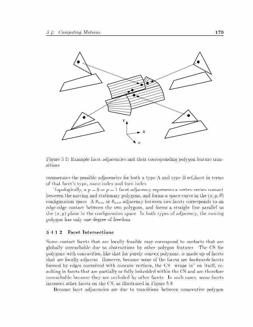
�� Computing Motions ���
θ
X
Y
Figure �� � Example facet adjacencies and their corresponding polygon feature tran�sitions�
enumerates the possible adjacencies for both a type A and type B ref facet in termsof that facet�s type� move index and turn index�
Topologically� a p " or p " � facet adjacency represents a vertex�vertex contactbetween the moving and stationary polygons� and forms a space curve in the �x� y� ��con�guration space� A �min or �max adjacency between two facets corresponds to anedge�edge contact between the two polygons� and forms a straight line parallel tothe �x� y� plane in the con�guration space� In both types of adjacency� the movingpolygon has only one degree of freedom�
������� Facet Intersections
Some contact facets that are locally feasible may correspond to contacts that areglobally unreachable due to obstructions by other polygon features� The CS forpolygons with concavities� like that for purely convex polygons� is made up of facetsthat are locally adjacent� However� because some of the facets are backwards facetsformed by edges convolved with concave vertices� the CS �wraps in� on itself� re�sulting in facets that are partially or fully imbedded within the CS and are thereforeunreachable because they are occluded by other facets� In such cases� some facetsintersect other facets on the CS� as illustrated in Figure ����
Because facet adjacencies are due to transitions between consecutive polygon
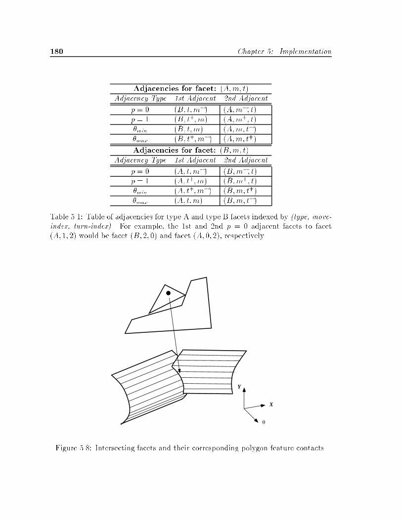
�� Chapter � Implementation
Adjacencies for facet� �A�m� t�Adjacency Type �st Adjacent �nd Adjacent
p " �B� t�m�� �A�m�� t�p " � �B� t��m� �A�m�� t��min �B� t�m� �A�m� t���max �B� t��m�� �A�m� t��
Adjacencies for facet� �B�m� t�Adjacency Type �st Adjacent �nd Adjacent
p " �A� t�m�� �B�m�� t�p " � �A� t��m� �B�m�� t��min �A� t��m�� �B�m� t���max �A� t�m� �B�m� t��
Table ���� Table of adjacencies for type A and type B facets indexed by �type� move�index� turn�index�� For example� the �st and �nd p " adjacent facets to facet�A� �� �� would be facet �B� �� � and facet �A� � ��� respectively�
θ
X
Y
Figure ���� Intersecting facets and their corresponding polygon feature contacts�
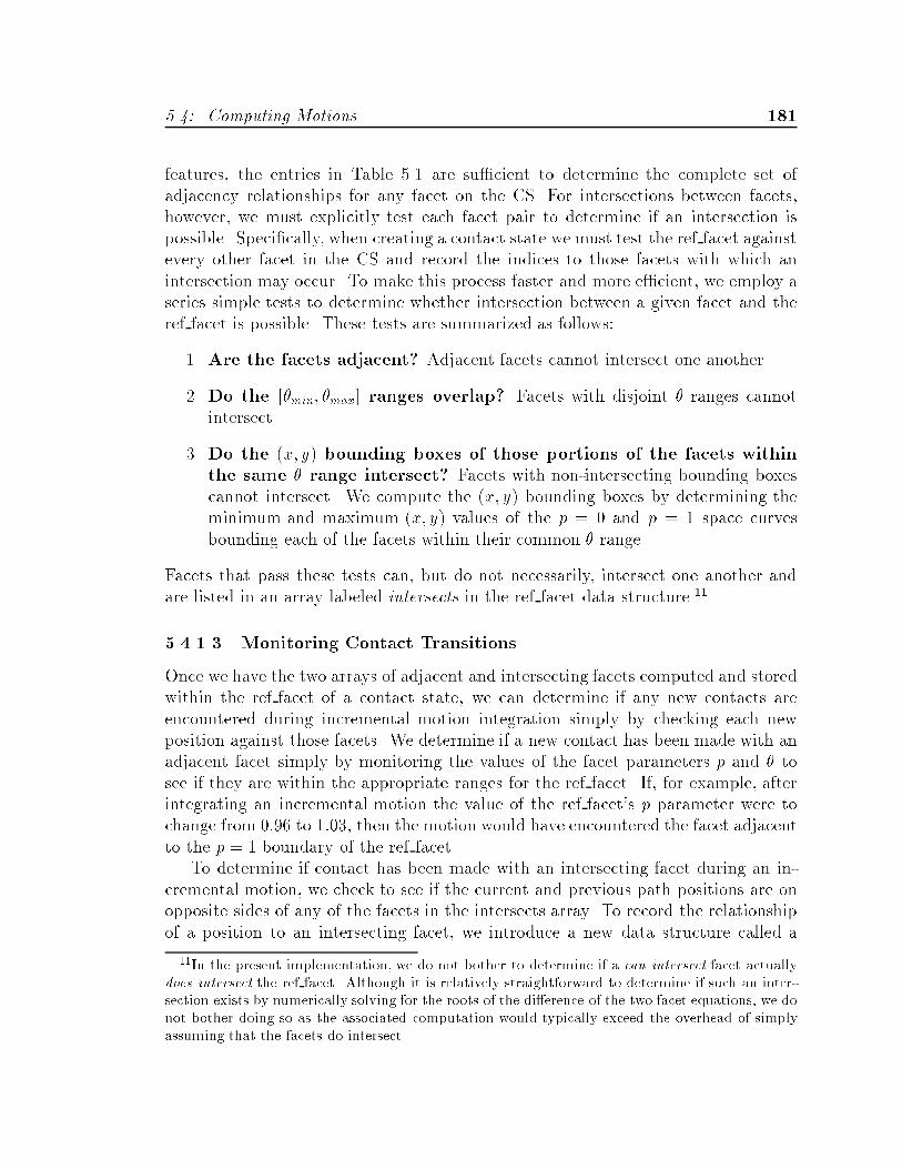
�� Computing Motions ���
features� the entries in Table ��� are su�cient to determine the complete set ofadjacency relationships for any facet on the CS� For intersections between facets�however� we must explicitly test each facet pair to determine if an intersection ispossible� Speci�cally� when creating a contact state we must test the ref facet againstevery other facet in the CS and record the indices to those facets with which anintersection may occur� To make this process faster and more e�cient� we employ aseries simple tests to determine whether intersection between a given facet and theref facet is possible� These tests are summarized as follows�
�� Are the facets adjacent� Adjacent facets cannot intersect one another�
�� Do the ��min� �max� ranges overlap� Facets with disjoint � ranges cannotintersect�
�� Do the �x� y� bounding boxes of those portions of the facets withinthe same � range intersect� Facets with non�intersecting bounding boxescannot intersect� We compute the �x� y� bounding boxes by determining theminimum and maximum �x� y� values of the p " and p " � space curvesbounding each of the facets within their common � range�
Facets that pass these tests can� but do not necessarily� intersect one another andare listed in an array labeled intersects in the ref facet data structure���
������� Monitoring Contact Transitions
Once we have the two arrays of adjacent and intersecting facets computed and storedwithin the ref facet of a contact state� we can determine if any new contacts areencountered during incremental motion integration simply by checking each newposition against those facets� We determine if a new contact has been made with anadjacent facet simply by monitoring the values of the facet parameters p and � tosee if they are within the appropriate ranges for the ref facet� If� for example� afterintegrating an incremental motion the value of the ref facet�s p parameter were tochange from ��� to ���� then the motion would have encountered the facet adjacentto the p " � boundary of the ref facet�
To determine if contact has been made with an intersecting facet during an in�cremental motion� we check to see if the current and previous path positions are onopposite sides of any of the facets in the intersects array� To record the relationshipof a position to an intersecting facet� we introduce a new data structure called a
��In the present implementation we do not bother to determine if a can intersect facet actuallydoes intersect the ref facet� Although it is relatively straightforward to determine if such an inter�section exists by numerically solving for the roots of the di�erence of the two facet equations we donot bother doing so as the associated computation would typically exceed the overhead of simplyassuming that the facets do intersect�

��� Chapter � Implementation
θ
X
Y
on
above
below
crossing
Figure ���� Four proximal cases for a type B intersect facet� All four points shownhave the same � component�
proximal� A proximal for an intersecting facet records the signed �x� y� distance ofan �x� y� �� point in con�guration space to a line segment corresponding to a slice ofthe facet surface at that value of �� as well as a �ag indicating whether the pointis� above �i�e� outside� the facet surface� crossing the line containing the facet slice�but outside of the slice segment�s endpoints�� on the line containing the facet slice�within the segment�s endpoints�� or below �i�e� inside� the facet surface��� A transi�tion of a proximal �ag from above to below or from above to on would indicate thatthe incremental motion has crossed that proximal�s corresponding intersecting facet�Figure ��� illustrates the four states of a proximal �ag for an intersect facet�
When a new contact is made� a new contact state containing the larger set ofcontact facets must be generated� Speci�cally� the following steps are taken if� afteran integration step� changes in one or more facet parameter values or proximal �agsindicate that a new contact has been made�
�� Interpolate between the startpoint and endpoint of the integration step us�ing the previous and current facet parameter or proximal distance values todetermine the �x� y� �� point�s� at which facet�s� were crossed�
��The �ags crossing and on are assigned to points that are within a set minimumdistance positiveor negative� of the line containing the facet slice�
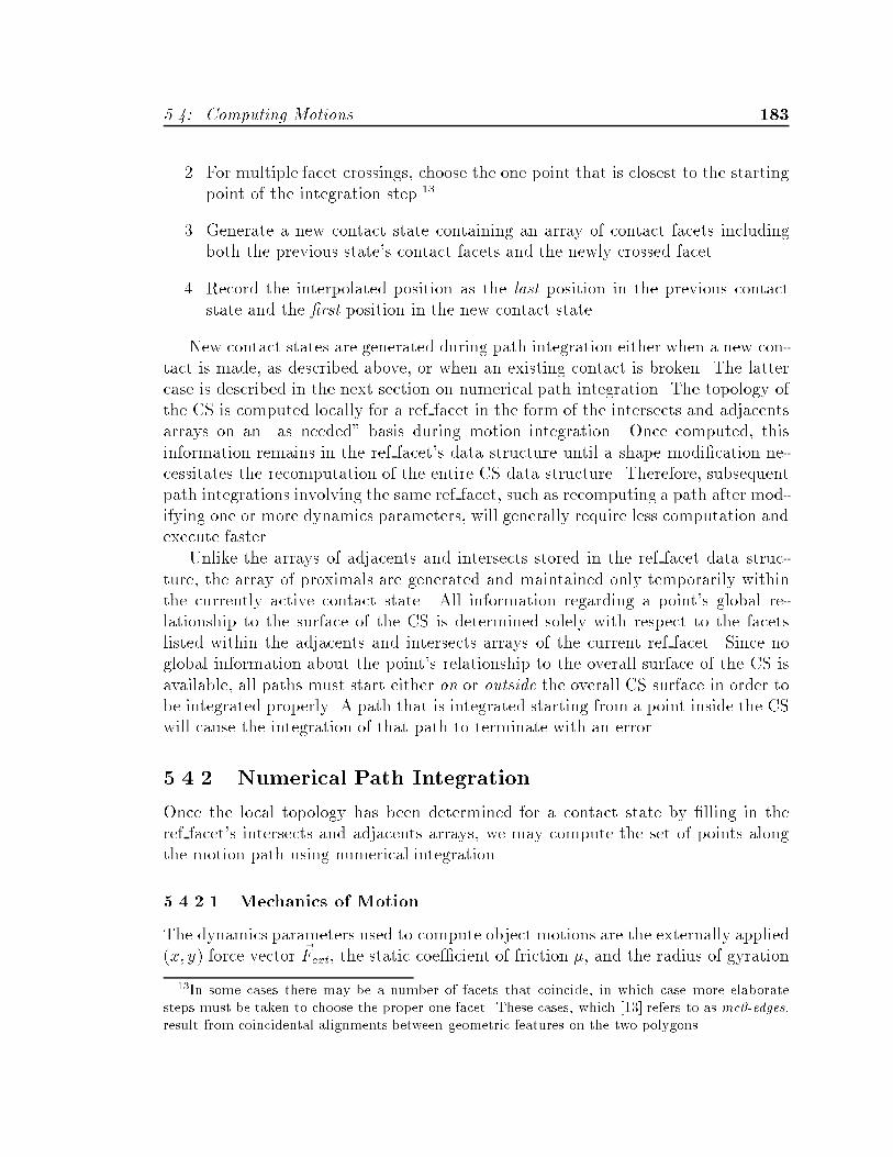
�� Computing Motions ���
�� For multiple facet crossings� choose the one point that is closest to the startingpoint of the integration step���
�� Generate a new contact state containing an array of contact facets includingboth the previous state�s contact facets and the newly crossed facet�
� Record the interpolated position as the last position in the previous contactstate and the �rst position in the new contact state�
New contact states are generated during path integration either when a new con�tact is made� as described above� or when an existing contact is broken� The lattercase is described in the next section on numerical path integration� The topology ofthe CS is computed locally for a ref facet in the form of the intersects and adjacentsarrays on an �as needed� basis during motion integration� Once computed� thisinformation remains in the ref facet�s data structure until a shape modi�cation ne�cessitates the recomputation of the entire CS data structure� Therefore� subsequentpath integrations involving the same ref facet� such as recomputing a path after mod�ifying one or more dynamics parameters� will generally require less computation andexecute faster�
Unlike the arrays of adjacents and intersects stored in the ref facet data struc�ture� the array of proximals are generated and maintained only temporarily withinthe currently active contact state� All information regarding a point�s global re�lationship to the surface of the CS is determined solely with respect to the facetslisted within the adjacents and intersects arrays of the current ref facet� Since noglobal information about the point�s relationship to the overall surface of the CS isavailable� all paths must start either on or outside the overall CS surface in order tobe integrated properly� A path that is integrated starting from a point inside the CSwill cause the integration of that path to terminate with an error�
����� Numerical Path Integration
Once the local topology has been determined for a contact state by �lling in theref facet�s intersects and adjacents arrays� we may compute the set of points alongthe motion path using numerical integration�
������� Mechanics of Motion
The dynamics parameters used to compute object motions are the externally applied�x� y� force vector Fext� the static coe�cient of friction �� and the radius of gyration
��In some cases there may be a number of facets that coincide in which case more elaboratesteps must be taken to choose the proper one facet� These cases which ���� refers to as mc��edgesresult from coincidental alignments between geometric features on the two polygons�

��� Chapter � Implementation
of the moving object� With these parameters we can compute the reaction forcesand static force equilibrium conditions for any point in a contact state� To combinethe units of force and torque consistently� we must �rst scale the torque componentsof the reaction forces with as�
Fz "�� �
Similarly� we scale the � components of the facet vectors with���
&uz " u��
where &u� was introduced in Section ������Computing an incremental motion step involves the following basic steps�
�� Compute the con�guration space friction cone at the current position in thecontact state representing the set of possible reaction forces�
�� Use the friction cone to compute the reaction force for the given applied force�
�� Compute the instantaneous direction of motion using the net resultant force�if any��
� Determine the appropriate integration step size and compute the incrementalmotion�
The detailed implementation of these four steps for computing motions in a free�facet� edge� and vertex contact state follows�Friction Cone Construction
To determine the set of possible reaction forces we construct the �x� y� z� con�g�uration space friction cone for each contacting facet� The friction cone for a singlefacet is shown in Figure ���� where n is the surface normal of the facet at the contactpoint� and Fr�� Fr� are the two extremal reaction forces that together span the rangeof reaction possible forces� The equations for Fr�� Fr� are�
Fr�x " ��nx cos�� ny sin�� ������
Fr�y " ���nx sin�� ny cos�� ���� �
Fr�z " ��nz cos �� � sin�� ������
Fr�x " ��nx cos�� ny sin�� ������
Fr�y " ��nx sin�� ny cos�� �����
Fr�z " ��nz cos �� � sin �� ������
��To ensure that the facet vectors remain unit vectors we normalize them after introducing thescaling factor ��

�� Computing Motions ���
where
sin� "�p
� � ��������
cos � "�p
� � ��������
� "�q
�n�x � n�y������
� "
vuut�rc
��
��� n�z�� n�z ������
and where � is the coe�cient of friction� �nx� ny� nz� are the normalized componentsof the scaled facet normal� is the radius of gyration� and rc is the distance from thecg of the moving polygon to the point of contact� For a type B facet rc is a constantmeasured from the cg to the vertex of the moving polygon that is in contact withedge of the stationary polygon� and is given by�
rc "RA
j
������
where j is the turn index of the facet� For a type A facet the value of rc is a functionof the facet parameter p and is given by�
rc "RA
i�� � p EAi
���� �
where i is the move index of the facet�For contact states with multiple contact facets it will be necessary to combine
the friction cones for the individual facets to form the compound friction cone� Foran edge contact state �two facets� we form the compound friction cone from the
convex hull of the extremal friction cone reaction forces Fr� and Fr� for the twofacets� Speci�cally� we order the four extremal force vectors to form the edges ofa convex polyhedral cone as shown in Figure ����� We do not form the compoundfriction cone for a vertex contact because� by de�nition� a vertex has zero degrees offreedom and hence no sliding motion is possible� We do� however� check for possiblemotions along the three edges forming the vertex to see if a motion out of the vertexis possible� as described in Section ������� Finally� for a free contact state �no facets�there can be no reaction forces and hence no friction cone�Computation of Reaction Forces
After constructing the friction cone for a contact state� we use it to compute thereaction force due to the applied force� The reaction force for a single facet contactis determined by projecting the negated applied �x� y� force onto the �x� y� fz " �g�plane containing the con�guration space friction cone� If the projected force vectoris between the two extremal friction cone reaction force vectors then the reaction

��� Chapter � Implementation
X
Y
θ
X
Y
ncsFr1
Fr2
rc
Figure ���� The �x� y� fz " �g� con�guration space friction cone for a single facetcontact�
Fx Fy
Fz = τθ / ρ
Fr1b
Fr1a Fr2
b
Fr2a
Fx Fy
Fz = τθ / ρ
Fr1b
Fr1a
Fr2b
Fr2a
Figure ����� The compound con�guration space friction cone for an edge contactbetween two facets�

�� Computing Motions ���
Fx Fy
Fz = τθ / ρ
Fr1
Fr2
Fnet
- Fext
Freact
Figure ����� Computing the reaction force with the single facet friction cone�
force is the projected force vector� If the projected force vector is not between thetwo extremal force vectors� then the reaction force is equivalent to the projection ofthe projected force onto the closer of the two extremal force vectors� This process isillustrated in Figure �����
To determine the reaction force for an edge contact� we �rst check to see if theapplied force is pointing into the compound cone by taking the dot�product of theforce with the outward pointing normals of each of the four bounding planes of theconvex cone� If all four dot�products are positive� the applied force points into thecone interior and the reaction force is exactly the negated applied force� If oneor more of the dot�products is negative� then the applied force lies outside of thecompound polyhedral cone� an we must project the negative applied force onto thesurface of the cone� Speci�cally� we project the negated applied force onto eachthe surfaces of the cone with which the dot�product was negative� and proceed in amanner similar to that for the single facet friction cone�Computation of Instantaneous Motion Direction
To compute the force equilibrium state at the contact point we compute the netforce by taking the di�erence between the applied and reaction forces� A non�zeronet force vector determines the instantaneous direction of motion from the currentcontact point� For a free contact state there is no reaction force so the net force issimply the applied force� For a single facet contact state a non�zero net force will betangent to the facet surface� and the non�zero net force for an edge contact will be

��� Chapter � Implementation
parallel to the edge vector formed by the cross�product of the two facet normals atthe contact point�Computation of Integration Step Size and Incremental Motion
Following our assumption that quasi�static e�ects dominate the dynamics of ob�ject motion� we may write the following equations of motion�
Fx " m'x � lim�t�
m(x
(t�������
Fy " m'y � lim�t�
m(y
(t�������
Fz "��
"I
'� � lim
�t�
I
(�
(t�����
where �Fx� Fy� Fz� are the components of the net force at the point of contact� and(t is a time step that will chosen to scale the magnitude of the incremental motionappropriately���
A motion in a free contact state will follow a straight line parallel to the appliedforce in the absence of any externally applied torques� which we have assumed in ourmodel� An incremental motion in a single facet contact state will be in the directionof the net force� but should also remain on the surface of the facet in the course ofthe motion even though the surface may be curved� To ensure this� and at the sametime avoid introducing linearization errors� we resolve the net force into componentsexpressed in the u and v tangent vectors of the facet surface� and integrate theincremental motion in terms of the p and � facet parameters�
To distinguish between displacements in translation and rotation� we denote thecombined displacement in x and y as xy� which can be expressed in terms of the facetparameter p as xy " lp where l is the length of the polygon edge forming the contactfacet� Substituting m " I
�into the above equations we can write the rotational and
translational displacements in terms of the facet parameters as�
(p "�
l
�(t�
m
�Fxy �����
(� "�
�(t�
m
�Fz� �����
To compute the instantaneous direction of motion we may normalize (p and (�
��Due to the quasi�static assumption the magnitude of the integration step may not be deter�mined directly from the equations of motion as would be the case for standard Euler or Runge�Kutta numerical integration techniques� Rather the integration step size will be derived from aconsideration of the errors produced by straight line approximations to motions along the surfacesof curved contact facets� Hence integration step size like the friction cone is computed directlyfrom contact facet geometry�
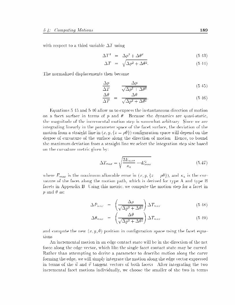
�� Computing Motions ���
with respect to a third variable (T using
(T � " (p� �(�� �����
(T "q(p� �(��� ����
The normalized displacements then become
(p
(T"
(pp(p� �(��
�����
(�
(T"
(�p(p� �(��
� �����
Equations ��� and ��� allow us to express the instantaneous direction of motionon a facet surface in terms of p and �� Because the dynamics are quasi�static�the magnitude of the incremental motion step is somewhat arbitrary� Since we areintegrating linearly in the parameter space of the facet surface� the deviation of themotion from a straight line in �x� y� fz " �g� con�guration space will depend on thedegree of curvature of the surface along the direction of motion� Hence� to boundthe maximum deviation from a straight line we select the integration step size basedon the curvature metric given by�
(Tmax "
s�Emax
�n� E�
max ��� �
where Emax is the maximum allowable error in �x� y� fz " �g�� and �n is the cur�vature of the facet along the motion path� which is derived for type A and type Bfacets in Appendix B� Using this metric� we compute the motion step for a facet inp and � as�
(Pmax "
�(pp
(p� �(��
�(Tmax �����
(�max "
�(�p
(p� �(��
�(Tmax �����
and compute the new �x� y� �� position in con�guration space using the facet equa�tions�
An incremental motion in an edge contact state will be in the direction of the netforce along the edge vector� which like the single facet contact state may be curved�Rather than attempting to derive a parameter to describe motion along the curveforming the edge� we will simply integrate the motion along the edge vector expressedin terms of the u and v tangent vectors of both facets� After integrating the twoincremental facet motions individually� we choose the smaller of the two in terms

�� Chapter � Implementation
of total distance in �x� y� �� con�guration space for the edge motion� and removeany linearization error by projecting the new point onto the edge between the facetscalculated at the new value of ���� This is a rather crude approximation to the actualedge motion� but it eliminates having to compute the incremental motion along anedge curve that might be di�cult or impossible to compute in closed form� Sinceintersection curves between facets may have a much higher degree of curvature thanthe facets themselves� this approximation is a recognized weak point of the currentmotion path integration implementation�
������� Selecting Consistent Motions
The computations for integrating motion in each of the four types of contact state�free� facet� edge� vertex� assume that resulting motion will maintain all of the con�tacts in that state� For example� computing the motion in a single facet contactstate in terms of the facet parameters p and � does not take into account the pos�sibility that the given applied force will cause the motion to leave the facet surface�To ensure that the computed incremental motions are consistent� we must check tomake sure that the assumptions implicit in the equations of motion are in fact valid�
A free motion� by de�nition� involves no contacts and hence is always consistentgiven a non�zero applied force� A facet motion is consistent if the applied forcepoints into the facet surface at the initial position of the integration� This may bechecked by computing the dot�product of the applied force vector with the facet�snormal vector at that point� A negative value indicates that the force points into thefacet surface and any motion must take place on the facet� whereas a positive resultindicates the motion will leave the facet surface�
An edge motion is consistent if the motions due to the applied force on the twofacets forming the edge both point into that edge� We may check this by computingthe vector tangent to each facet�s surface that is perpendicular to the edge vectorand taking the dot�product of the corresponding facet motions with each of thesevectors� A positive value for either dot�product would indicate that the resultingmotion would break contact with the other facet and become a single facet motion�
Finally� we can determine if a motion into or out of a contact state for a vertexformed by three facets is possible by checking if a motion along any of the three edgesintersecting at the vertex points away from the vertex� If all three edge motions pointinto the vertex then no motion is possible and integration is terminated� Otherwisea consistent edge motion must be selected�
In each of the above cases� if the incrementalmotion in the current contact state isfound to be inconsistent� we generate a new contact state with the next lower numberof contacts �one greater degree of freedom�� and store the current position as the last
��If the edge is a straight line such as a �min or �max adjacency then there the new position hasthe same � component as the old position and no linearization is necessary�

�� Computing Motions ���
point in the previous state and the rst point in the new state� Figure ���� illustratesthe above motion selection procedures for the four types of contact state�
������� Computing Initial Conditions
There are two types of initial conditions used for integrating motions in cspace�shell�the choice of which depends on the application domain� To �nd the initial conditionsfor part motions through a vibratory feeder� we identify the set of stable initial ori�entations of the moving object in contact with the bowl wall� We construct this set�which corresponds to the possible orientations in which a part may enter the feeder�by �rst taking the convex hull of the moving polygon and generating an edge contactstate for each pair of vertices on the convex hull� Each contact state contains thepair of contact facets corresponding to a contact between one of the two vertices andthe top leftmost horizontal edge of the stationary polygon along which parts enterthe feeder� The stability of each edge contact state is then evaluated by computingthe reaction forces at the two contact points that are necessary to maintain staticequilibrium with an applied force through the polygon�s cg pointing along the �yaxis� as illustrated in Figure ���� If one of the reaction forces is negative ��y�� thenthe orientation is unstable� and the contact state is removed�
For feeder design purposes� it would be helpful to know the probability withwhich a part in a given orientation will enter the feeder� We compute the probabilityassociated with each stable contact state by assuming a uniform probability distri�bution over the � " � � �� range of orientations in which a part may �rst comeinto contact with the bowl wall� and then dividing this range into � regions in whichthe part would tend toward a given stable orientation� The widths of the resulting �ranges are then divided by � to obtain the probability � � �� of a part appearingin that orientation� Figure ���� illustrates this process using the radius function ofa part�
To integrate more general object motions� such as a part being placed into asubassembly� we allow the user to select an arbitrary �x� y� �� position correspondingto a free contact state� or a point on a facet surface corresponding to a facet contactstate� The free �x� y� �� position is selected using three position sliders� and is graph�ically displayed in con�guration space as the intersection of three lines parallel tothe �x� y� �� axes� The free contact state generated for this position uses a temporarynull facet data structure containing all of the facets in the CS within the intersectsarray��� The user is responsible for selecting a position that is on the outside of theCS�
A position in a facet contact state is selected by having the user click the mouseover a displayed facet� The position is mapped from �x� y� �� to the corresponding
��Strictly speaking the free region in con�guration space intersects all of the facets in the CS�
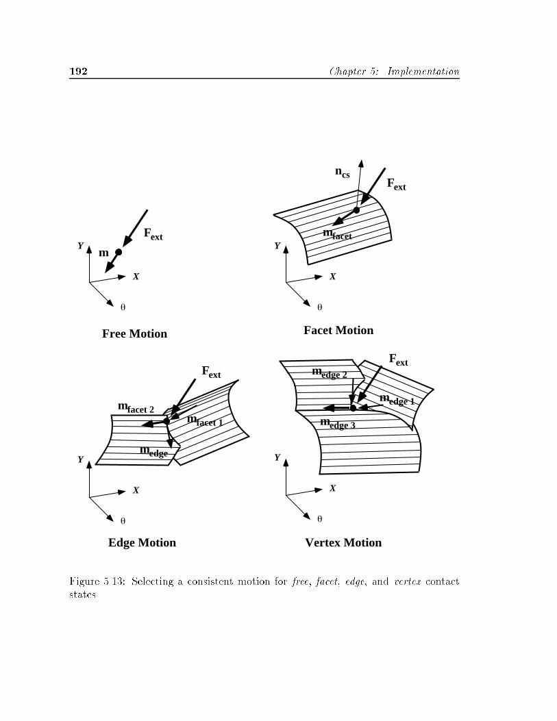
��� Chapter � Implementation
θ
X
Y
θ
X
Y
θ
X
Y
θ
X
YFext
Fext
Fext
Fext
m
ncs
mfacet
mfacet 1
mfacet 2
medge
medge 1
medge 2
medge 3
Free Motion Facet Motion
Edge Motion Vertex Motion
Figure ����� Selecting a consistent motion for free� facet� edge� and vertex contactstates�
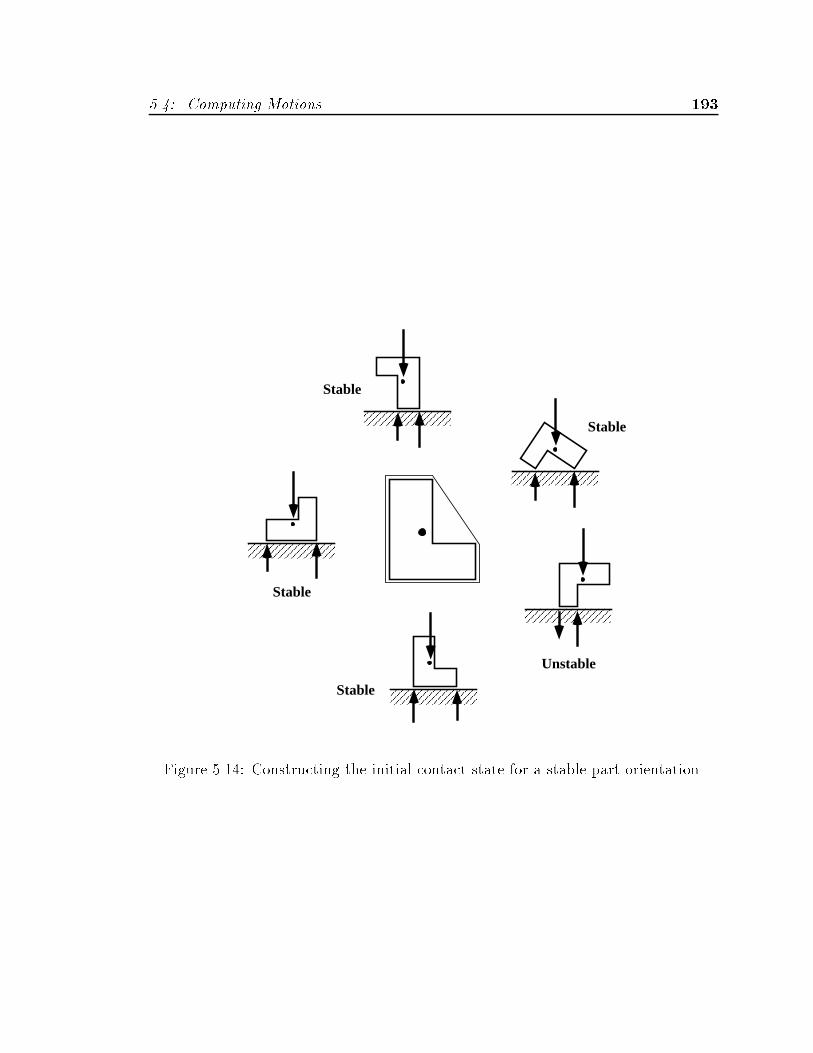
�� Computing Motions ���
Stable
Stable
Stable
Stable
Unstable
Figure ���� Constructing the initial contact state for a stable part orientation�
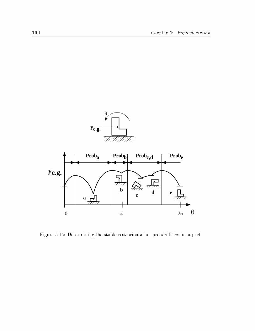
��� Chapter � Implementation
θ
π 2π0
a
bc d e
Proba Probb Probc,d Probe
yc.g.
yc.g.
θ
Figure ����� Determining the stable rest orientation probabilities for a part�

�� Computing Motions ���
�p� �� facet parameters and the facet contact state is initialized normally as describedin earlier sections� The mouse based selection routine is described in Section �� �
������� Iterative Stepwise Integration
All of the motion computation operations discussed above are combined within anincremental motion path integration loop that is executed on command by the user�
For each initial contact state we execute the following procedure�
path integration loop��
compute proximals�� Compute the array of proximals determining the rela�tionship between the current position and the neighboring adjacent andintersecting facets�
Begin loop Begin the incremental motion integration loop�
test motion termination�� Check to see if current position is outsideof the �x� y� �� motion bounding box� If there is a support map checkto see if the current position is supported�
integrate motions�� Integrate the incrementalmotion from the currentposition� including any sub�motions required to check for motion con�sistency�
select motion�� Select the consistent motion�
If there is no motion� exit with no motion �ag�
If the motion has left any existing contacts�
create contact state�� Create a new contact state correspondingto the reduced set of contact facets�
compute proximals�� Recompute the array of proximals for the oldposition in the new contact state�
record and increment position�� Record the current position asthe �rst position in the new contact state�
current state � new state Continue with the new contact state�
compute proximals�� Compute the array of proximals for the new posi�tion in the contact state�
detect new contact�� Compare the old and new proximals to determineif a new contact has been made� and select a single new contact facetif necessary�
If no new contact was made� then�
record and increment position�� Record the new position in thecontact state�
��� Chapter � Implementation
Else� if a new contact was made�
record and increment position�� Record the new position as thelast position in the current contact state�
create contact state�� Create a new contact state correspondingto the larger set of contact facets�
compute proximals�� Recompute the array of proximals for the newposition in the new contact state�
record and increment position�� Record the new position as the�rst position in the new contact state�
Go To Begin loop
End
Upon exiting� path�integration�loop�� returns a �ag indicating the mode ofpath termination which is one of�
� no motion � Motion has stopped at a vertex or due to sticking�
� loss of support � The motion is in an unsupported region of the CS�
� outside motion bbox � The motion has left the allowable region of �x� y� ��con�guration space�
� error � error code � An error identi�ed by error code has occurred withinpath�integration�loop���
We have now described all of the major components required to construct motionpaths in con�guration space�
��� Computing Support Transitions
����� Assumptions
The following is a list of the assumptions made in computing the support status ofpoints on the surface of the CS�
� The moving objects are assumed to be �at� fully planar polygons with negligiblethickness�
� The reference point representing the center of gravity �cg� through which allexternal forces are applied to the part is assumed to lie within the contour ofthe part�
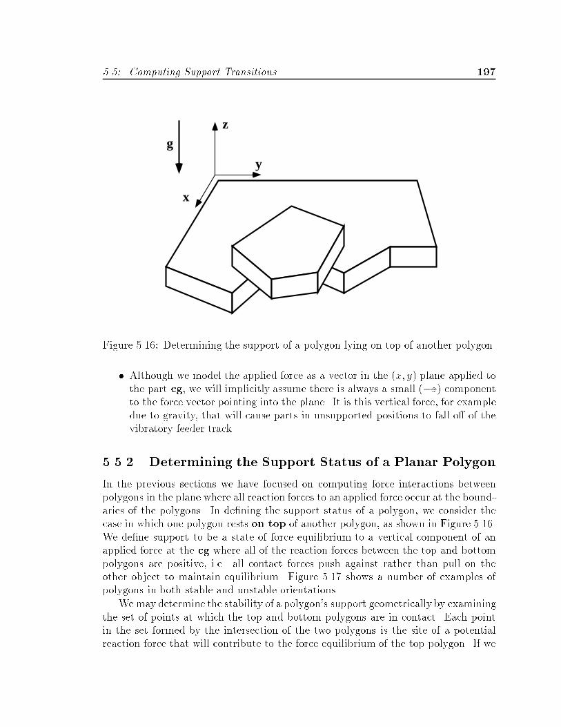
�� Computing Support Transitions ���
x
y
z
g
Figure ����� Determining the support of a polygon lying on top of another polygon�
� Although we model the applied force as a vector in the �x� y� plane applied tothe part cg� we will implicitly assume there is always a small ��z� componentto the force vector pointing into the plane� It is this vertical force� for exampledue to gravity� that will cause parts in unsupported positions to fall o� of thevibratory feeder track�
����� Determining the Support Status of a Planar Polygon
In the previous sections we have focused on computing force interactions betweenpolygons in the plane where all reaction forces to an applied force occur at the bound�aries of the polygons� In de�ning the support status of a polygon� we consider thecase in which one polygon rests on top of another polygon� as shown in Figure �����We de�ne support to be a state of force equilibrium to a vertical component of anapplied force at the cg where all of the reaction forces between the top and bottompolygons are positive� i�e� all contact forces push against rather than pull on theother object to maintain equilibrium� Figure ��� shows a number of examples ofpolygons in both stable and unstable orientations�
We may determine the stability of a polygon�s support geometrically by examiningthe set of points at which the top and bottom polygons are in contact� Each pointin the set formed by the intersection of the two polygons is the site of a potentialreaction force that will contribute to the force equilibrium of the top polygon� If we
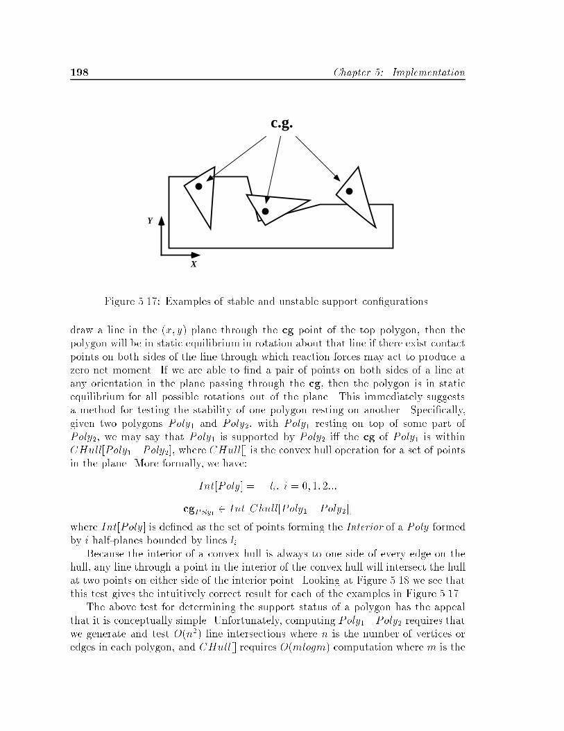
��� Chapter � Implementation
X
Y
c.g.
Figure ��� � Examples of stable and unstable support con�gurations�
draw a line in the �x� y� plane through the cg point of the top polygon� then thepolygon will be in static equilibrium in rotation about that line if there exist contactpoints on both sides of the line through which reaction forces may act to produce azero net moment� If we are able to �nd a pair of points on both sides of a line atany orientation in the plane passing through the cg� then the polygon is in staticequilibrium for all possible rotations out of the plane� This immediately suggestsa method for testing the stability of one polygon resting on another� Speci�cally�given two polygons Poly� and Poly�� with Poly� resting on top of some part ofPoly�� we may say that Poly� is supported by Poly� i� the cg of Poly� is withinCHull�Poly��Poly��� where CHull�� is the convex hull operation for a set of pointsin the plane� More formally� we have�
Int�Poly� "li� i " � �� ����
cgPoly� � Int �Chull�Poly� � Poly���where Int�Poly� is de�ned as the set of points forming the Interior of a Poly formedby i half�planes bounded by lines li�
Because the interior of a convex hull is always to one side of every edge on thehull� any line through a point in the interior of the convex hull will intersect the hullat two points on either side of the interior point� Looking at Figure ���� we see thatthis test gives the intuitively correct result for each of the examples in Figure ��� �
The above test for determining the support status of a polygon has the appealthat it is conceptually simple� Unfortunately� computing Poly��Poly� requires thatwe generate and test O�n�� line intersections where n is the number of vertices oredges in each polygon� and CHull�� requires O�mlogm� computation where m is the
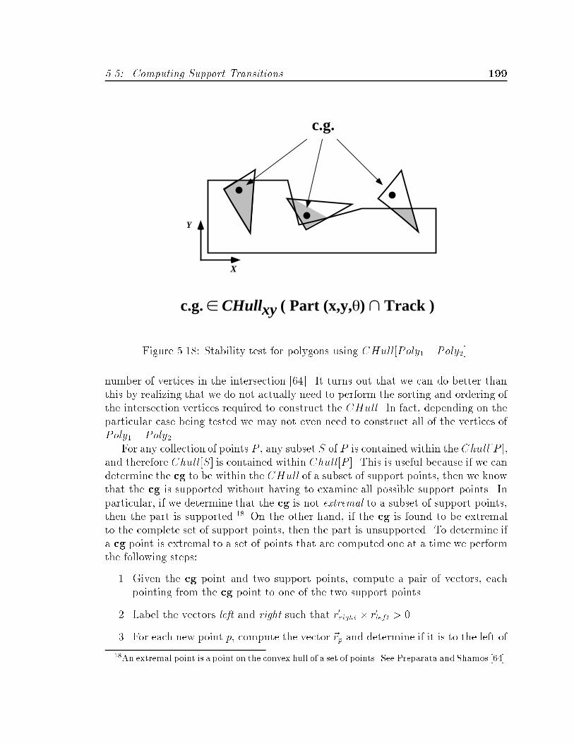
�� Computing Support Transitions ���
c.g. ∈ CHullxy ( Part (x,y,θ) ∩ Track )
X
Y
c.g.
Figure ����� Stability test for polygons using CHull�Poly� � Poly���
number of vertices in the intersection ���� It turns out that we can do better thanthis by realizing that we do not actually need to perform the sorting and ordering ofthe intersection vertices required to construct the CHull� In fact� depending on theparticular case being tested we may not even need to construct all of the vertices ofPoly� � Poly��
For any collection of points P � any subset S of P is contained within the Chull�P ��and therefore Chull�S� is contained within Chull�P �� This is useful because if we candetermine the cg to be within the CHull of a subset of support points� then we knowthat the cg is supported without having to examine all possible support points� Inparticular� if we determine that the cg is not extremal to a subset of support points�then the part is supported��� On the other hand� if the cg is found to be extremalto the complete set of support points� then the part is unsupported� To determine ifa cg point is extremal to a set of points that are computed one at a time we performthe following steps�
�� Given the cg point and two support points� compute a pair of vectors� eachpointing from the cg point to one of the two support points�
�� Label the vectors left and right such that rright � rleft � �
�� For each new point p� compute the vector rp and determine if it is to the left of
��An extremal point is a point on the convex hull of a set of points� See Preparata and Shamos �����

� Chapter � Implementation
rleft or to the right of rright by taking the cross products of the respective vectorswith rp and checking the sign of the result� If a sign change occurs� replace thecorresponding left or right vector with rp� and recompute rright � rleft�
� If the cross product changes sign� i�e� becomes negative� then the cg point isno longer extremal to the set of points tested� and the part is supported�
�� Else� compute the next support point p and go to step ��
�� If there are no more support points to test� and rright � rleft � � then the cgpoint is extremal to the set of support points and the part is unsupported�
This process is illustrated in Figure �����By testing each point in Poly� �Poly� as it is generated� we improve the average
performance of the overall support test because as soon as we generate a point thatplaces the cg in the interior of the existing set of intersection points we can stop andreport the part to be supported� In the worst case� which will occur when the cgis in fact unsupported� our test is still O�n�� because we will have to generate andtest every point in Poly� � Poly� since we never know when the next point in theintersection might make the cg point no longer extremal�
����� Approximations and Optimizations
On average the extremal point test provides a considerable improvement in comput�ing the support status of a point in con�guration space� Nevertheless� computingsupport regions by simply testing and labeling as supported or unsupported discretepoints would be unacceptably slow for an interactive design environment� In thissection we discuss a series of hierarchical tests and optimizations that can reduceeven further the amount of necessary computation�
To begin with� we will compute the support status of only those con�gurationspace points that lie on the surface of facets in the CS� and as was the case for motioncomputation we will not explicitly represent edges or vertices on the CS� Anothersimpli�cation arises from the observation that� assuming the cg is contained withinthe contour of the part� the part will be supported if the cg point lies within theinterior of the support polygon� Similarly� if the cg point lies outside of the CHull��of the supporting polygon� then no support is possible since there can be no supportpoints outside the support polygon�s CHull��� For a given position of a part�s cg wecan compute the state of the cg point with respect to the support polygon and itsconvex hull� Table ��� lists the possible cg states and their resulting support status�
The main advantage of this test is that we need only compute the status of apoint with respect to the support polygon� as opposed to computing the intersectionof both the part polygon and support polygon� Since a facet surface represents the

�� Computing Support Transitions ��
( i ) ( i i ) ( i i i )
( iv ) (v) (v i )
Supported
c.g.
Figure ����� Testing the cg point against a series of points to determine if the cg isextremal�

�� Chapter � Implementation
Support Status from Point In Poly� Tests for Part cg�
cg in Support Poly� cg in CHull�Support Poly�� Part Support Status
Point Outside Point Outside UnsupportedPoint Outside Point Inside Test SupportPoint Inside Point Outside �Point Inside Point Inside Supported
Table ���� Table of part support status as determined by Point In Poly� status ofthe part cg w�r�t� the Support Poly and CHull� Support Poly ��
set of possible positions of the part cg for a given contact� the Point In Poly� testalso allows us to hierarchically test for support starting �rst with an entire facet� andthen smaller subregions within a facet determined by ranges of �p� ��� Only in thosecases where the result is Test Support will we need more extensive and detailedtesting using the extremal point routine�
Testing a Whole Facet�s Support Status�
We �rst determine if an entire facet may be supported or unsupported by checkingthe facet�s bounding box against both the Support Poly and the CHull� Sup�port Poly ��� If the bounding box is inside of the Support Poly or outside of theCHull� Support Poly � then the part is supported or unsupported� respectively�over the range of positions determined by the facet�s surface� If the bounding boxintersects either of the polygons� or is between the Support Poly and the CHull�Support Poly �� then the facet�s support status must be examined in more detail�
Testing Regions of a Facet�
For those facets that intersect either the Support Poly or theCHull� Support Poly�� we must subdivide the surface of the facet into regions of di�ering support status�For simplicity� we choose to divide the facet into strips of �xed resolution that willbe tested individually� To do this more e�ciently� we �rst cache the intersectingpolygon segments from the bounding box test for later use to reduce the amount ofsubsequent testing required� Then� based on the facet�s size and curvature as givenby l �the length of the polygon edge forming the contact facet� and rc �the distancefrom the cg of the moving polygon to the point of contact�� we determine the maxi�mum (p and (� increments that are within the RESxy speci�ed for computing thesupport status over a facet�s surface� Using this information we divide the facet intoa series of �x� y� slices at increments of (� within ��min� �max�� Each of these slices
�We compute the x� y� bounding box of the facet over the range ��min� �max��

� � Rendering and Display ��
corresponds to a line segment in �x� y�� and represents a translation of the part cgalong a contact edge at a �xed orientation�
Testing Along a Facet Slice�
For each (� increment� we generate the facet slice line segment and test it for inter�sections with the polygon segments fromSupport Poly andCHull� Support Poly� that were cached in the facet�s bounding box test� All intersections are recordedand sorted by the value of the parameter p at which they intersect the facet seg�ment� The Point In Poly� status of the facet segment�s start point �p " � isthen computed� and the segment is divided into Supported� Unsupported� TestSupport� ranges by appropriately toggling the point status from p " at eachintersection with the segment from p � �� �� and labeling each following range ac�cordingly� Figure ��� illustrates this labeling process for a typical facet slice� Eachsegment range labeled Test Support must be explicitly tested at (p increments us�ing the extremal point test discussed earlier� and neighboring incremental test pointswith the same resulting support status are then merged� The �nal result is a facetslice line segment divided into a series of consecutive Supported or Unsupportedsub�ranges� whose adjacency points correspond to support transitions�
Each facet slice containing a support transition is recorded as an element in anarray of slices indexed by �slice� Each slice element in turn contains the supportstatus of the �p " � point of the slice� and an array of support transition �ags Lose Support� Gain Support � indexed by ptransition that indicate the type ofsupport transition� This array of arrays� illustrated in Figure ����� is stored in thefacet�s support map �eld� The support map is used both by the rendering routines todisplay the supported and unsupported regions of the facet� as well as by the motioncomputation routines to determine if a path has entered a ref facet�s unsupportedregion� Speci�cally� for each point generated along a motion path� we check thecorresponding �p� �� position on the ref facet against the support map to determineif that point is unsupported and should therefore be terminated��
��� Rendering and Display
Each facet surface is rendered in the �x� y� �� con�guration space as a series of poly�gons� each bounded by four vertices� Using a constant predetermined (�� the facetis divided into equally spaced slices from � " ��min� �max�� each of which is boundedby a pair of �x� y� �� vertices computed from the facet equations at p " and p " ��Each polygon structure points to two consecutive pairs of vertices� along with their
�For those portions of a path that are in free con�guration space we must test each incrementalpoint along the path explicitly using the extremal point test since no support map is available�
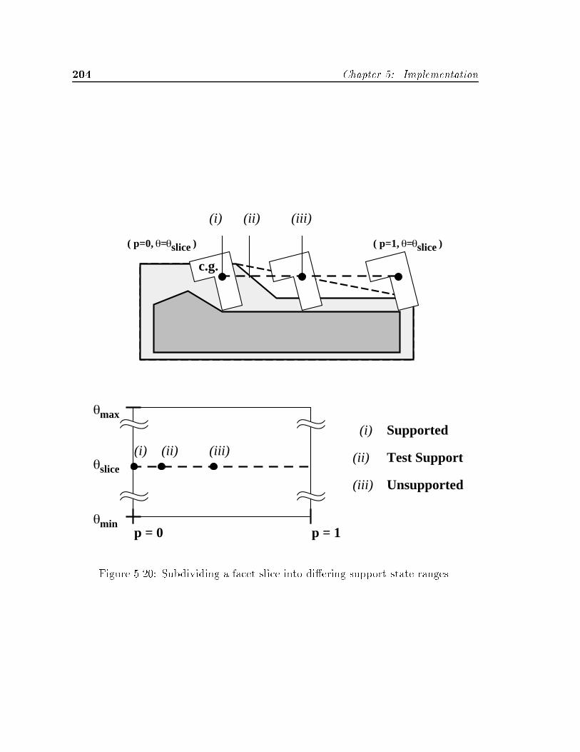
�� Chapter � Implementation
c.g.
(i) (ii) (iii)
(i) (ii) (iii)
p = 0 p = 1θmin
θmax
θslice
(i)
(ii)
(iii)
Supported
Test Support
Unsupported
( p=0, θ=θslice ) ( p=1, θ=θslice )
Figure ���� Subdividing a facet slice into di�ering support state ranges�

� � Rendering and Display ��
p = 0 p = 1
θmin
θmax Supported
Supported
UnsupportedActualBoundary
ApproximateBoundary
∆θ
Figure ����� A typical support map for a facet in terms of �p� ���
corresponding facet normal vectors� arranged counterclockwise around the outwardfacet normal� In addition to the vertices and normals� each polygon structure con�tains indices to the edge and vertex of the moving and stationary object polygonsthat form the contact facet� as well as indices to the palette of colors and materiallighting properties used to render the polygon� When enabled by the user� each poly�gon is drawn with a dark boundary line to highlight the facet contour� Otherwise�the polygons making up each facet are simply drawn and blended using the Phongshading model in the Silicon Graphics GL rendering library�
Each complete forward facet is rendered individually��� Those facets or portionsof facets that are occluded in the complete CS set are hidden from view by the depthbu�er� or Z�bu�er� of the graphics workstation� When motion paths are computedin con�guration space� they are rendered as curves composed of line segments con�necting the points along the path� and are drawn slightly above the surface of theCS facets� The line thickness of each path is drawn proportional to the probabilityof the initial position for that path so that the more common part motion paths arethicker than the less likely ones�
��Backward facets are by de�nition interior to the set of CS facets and hence will be hidden fromall viewing angles�

�� Chapter � Implementation
�� Interactive Design Functions
With the exception of specifying �le names via the keyboard� all user inputs tocspace�shell are made via the mouse� Vertices of the object polygons �part� bowlwall� and track� may be selected directly within the object display windows or indi�rectly from the CS in the con�guration space display window� Non�shape parameters�such as the coe�cient of friction � or the free�space start position for the computationof a single motion path� are modi�ed using simple linear sliders�
When the user selects a CS feature by clicking the mouse in the con�gurationspace display window� the X�Y position of the cursor in the window is transformedinto a line in the con�guration space coordinate system corresponding to the currentview using the Silicon Graphics mapw library function� This line is then tested forintersections with every facet rendering polygon in the CS that is visible� i�e� facingthe user� The intersected facet rendering polygon that is closest to the viewer isdetermined� and the facet type� index to the nearest rendering polygon vertex� andthe approximate �x� y� �� position selected on the facet surface is recorded�
Parametric Design Functions�
The information obtained from the selected vertex of the rendering polygon in theCS may be used to identify either the contacting object vertex or edge vertices thatform the corresponding selected facet� We determine which feature will be selectedby a priori assigning edge vertices of the moving object polygon to type A facets andedge vertices of the stationary polygon to type B facets� Therefore� the index numberreturned by the selected vertex of the rendering polygon may be used to select thecorresponding vertex of an object polygon� To make this coupling apparent to theuser� all of the facets in the CS that are a�ected the selected object vertex arehighlighted along with the vertex itself� This is accomplished by changing the colorpalette index of every rendering polygon in the CS that corresponds to the selectedobject vertex�
The user may move all of the currently selected object vertices together by se�lecting a point in con�guration space and moving away from it with the right mousebutton held down� In this case� an �x� y� plane is displayed in the con�gurationspace at the � value where the user initially clicked on the CS� Movements of themouse from this point are translated into incremental �x� y� motions by intersectingthis plane with the mapw line from the new mouse position� The �x� y� motions areapplied directly to all selected vertices of the stationary polygon� and inversely viaan inverse rotation matrix at the �x� y� plane�s � value� i�e� Rot������ to all selectedvertices of the moving polygon� The result is a change to the CS surface that tracksthe motion of the mouse in the �x� y� plane from the initial click point� along withthe modi�cations to the object vertices �shape� necessary to make this change to the
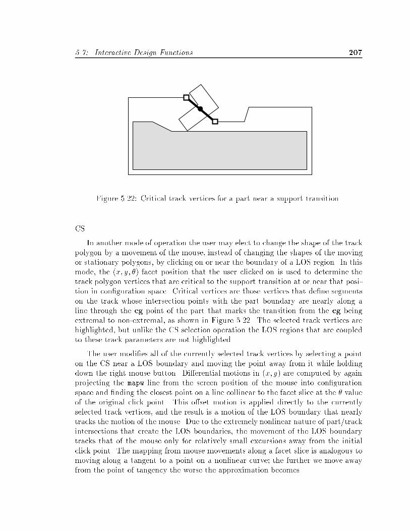
��� Interactive Design Functions ��
Figure ����� Critical track vertices for a part near a support transition�
CS�
In another mode of operation the user may elect to change the shape of the trackpolygon by a movement of the mouse� instead of changing the shapes of the movingor stationary polygons� by clicking on or near the boundary of a LOS region� In thismode� the �x� y� �� facet position that the user clicked on is used to determine thetrack polygon vertices that are critical to the support transition at or near that posi�tion in con�guration space� Critical vertices are those vertices that de�ne segmentson the track whose intersection points with the part boundary are nearly along aline through the cg point of the part that marks the transition from the cg beingextremal to non�extremal� as shown in Figure ����� The selected track vertices arehighlighted� but unlike the CS selection operation the LOS regions that are coupledto these track parameters are not highlighted�
The user modi�es all of the currently selected track vertices by selecting a pointon the CS near a LOS boundary and moving the point away from it while holdingdown the right mouse button� Di�erential motions in �x� y� are computed by againprojecting the mapw line from the screen position of the mouse into con�gurationspace and �nding the closest point on a line collinear to the facet slice at the � valueof the original click point� This o�set motion is applied directly to the currentlyselected track vertices� and the result is a motion of the LOS boundary that nearlytracks the motion of the mouse� Due to the extremely nonlinear nature of part�trackintersections that create the LOS boundaries� the movement of the LOS boundarytracks that of the mouse only for relatively small excursions away from the initialclick point� The mapping from mouse movements along a facet slice is analogous tomoving along a tangent to a point on a nonlinear curve# the further we move awayfrom the point of tangency the worse the approximation becomes�

�� Chapter � Implementation
Non�Parametric Design Functions�
The interactive functions described above all allow variational modi�cation only ofexisting design parameters� We may also introduce entirely new contours to the trackpro�le by generating a cutout from the track� The user selects a cutout by specifyingan �x� y� �� position from the CS and an oriented line in the �x� y� plane of the trackabout which a part should rotate out of the plane to fall o� the track� The motionof the part rotating out of the plane about this line produces a cutout contour inthe track corresponding to the shape of the part��� cspace�shell implements anapproximation to the cutout operation in which the generated cutout contour is theconvex hull of the actual contour that would be cut from the track as the part wasrotated out of the plane about the oriented line�
Using the selected �x� y� �� position and oriented �x� y� line� the cutout routinegenerates a polygonal contour around the intersection of the �x� y� �� translated androtated part contour and the half space to the right of the oriented line passingthrough the part cg� The convex hull of this contour is taken and expanded in�x� y� by the amount RESxy that is currently speci�ed for computing the supportstatus over a facet�s surface� The ordering of the expanded contour�s vertices arethen inverted to form a hole� and the polygon is intersected with the track polygonat the selected �x� y� position� If the cutout contour intersects the track boundary�it is cut and it�s vertices spliced into the track polygon� If the cutout contour iscompletely within the track polygon� the cutout vertex closest to the track edge issplit and connected to the track polygon via a narrow slot� The result in either caseis a new track polygon contour of genus zero� The cutout operation is illustrated inFigure �����
�� Summary
Based on the assumption that cspace�shellwould be used interactively on problemsof small to moderate size� i�e� polygons with O��� edges�vertices� our implemen�tation strategy focused on reducing the average running time required to computemotion constraints for such problems versus developing algorithms aimed at reducingthe asymptotic running time of larger problems�
�� �� Optimizations
Some of the major optimizations to improve the performance of cspace�shell andits subroutines that were discussed earlier are summarized here for reference�
��This contour is actually an approximation to the cross�section of the volume swept out by thepart as it rotates out of the plane to fall o� of the track�
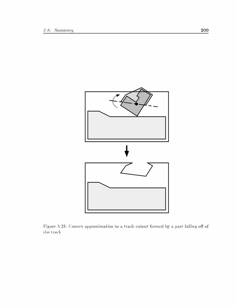
��� Summary ��
Figure ����� Convex approximation to a track cutout formed by a part falling o� ofthe track�

�� Chapter � Implementation
Generation and display of motion constraints�
� Compute and display only the CS facets during shape modi�cation� OtherCS features such as edges� vertices� and facets or portions of facets that areoccluded are left implicit�
� Use depth�bu�ering to hide occluded surfaces in the CS display�
Computation of paths and topology�
� Compute local CS topology only during motion path integration�
� Cache information on facet intersections and adjacencies in during path com�putation for use in subsequent path computations�
Computation of facet support maps�
� Test for support status using a hierarchy of tests from entire facets to sub�facetregions�
� Divide facets into regions of di�ering Point In Poly status of the part cg relativeto the track and CHull�� track polygons�
� Cache intersecting facet�track segments for use in repetitive support computa�tion and testing�
�� �� Complexity and Performance
Computational Complexity
The following are estimates of the worst case complexity for the three main processesrunning in cspace�shell� computation of contact facets� computation of supportregions �support maps� on the facets� and numerical integration of the motion paths�including the CS topology computation�� In actual usage� the optimizations listedabove combined with the inherent structure of the representations tend to makecomputations more tractable� as shown below� Each of the estimates below assumesthat all polygons have O�n� vertices�
Contact Facet Generation
Computation of a contact facet requires constant time and consists of computing afew constants and placing them into a data structure� A contact facet is generatedfor each edge�vertex and vertex�edge contact between two polygons� producing �n�
contact facets� The time complexity in terms of polygon size n is therefore O�n���
��� Summary ���
Support Map Computation
Computing the support map for a contact facet� in the worst possible case� consistsof testing whether or not the moving polygon�s cg is extremal to the set of possiblesupport points at the given �x� y� �� position of the moving polygon� This set consistsof the intersection of the moving and supporting polygons at that position� For twoarbitrary polygons there will be ��K�n�K�n log n� vertices to be tested� where K�
and K� are constants� Points are sampled across the facet at N "�ledge
�RESxy
�in�
tervals along M "�rcontact��max � �min�
�RESxy
��xed�� slices of the facet� Therefore�
the required computation is ��n���K�n �K�n log n�NM�� In terms of polygon sizen we have a time complexity of O�n� log n�� and in terms of resolution RESxy we
have O�
�RES�xy
��
Motion Path Integration
Computing motion paths consists of �rst determining and recording those facets thatmight be encountered through adjacent transitions or intersections with the currentreference facet� which is constant for computing adjacencies and requires K��n��
�
testing for facet intersections� where K is a constant� For each step in the integra�tion we must check for transitions relative to each of the C��n�� facets listed fromthe previous computation� where C � �� Integration steps are made at maximumintervals of the resolution given by RESxy� The actual motion computation at eachstep requires constant time Tcomp� Therefore� the computation required consists of�K��n��
�� Pcount
�RESxy
C��n���� which gives a worst case time complexity of O�n��
in terms of polygon size n� and in terms of resolution RESxy we have O�
�RESxy
��
Average Performance
The above complexity expressions are worst case bounds� The average time requiredto compute and render constraint facets for polygons on the order of � � � edgeswas � �� seconds� The average time required to compute and render support mapsfor the same polygons was � � � seconds for a resolution of �� inches� Finally� thetime required to compute motion paths for the same examples was � � seconds foran average of paths�

��� Chapter � Implementation

ConclusionChapter �
��� Summary
The primary goal of this research was to argue for the validity of the hypothesis thatmotion constraints can serve both as a representation of the function that may bederived from shape interactions and as a tool for manipulating and designing suchfunctional shapes�
We identi�ed and explored two key issues raised by the above hypothesis� thedevelopment of representations for function in terms of motion constraints� and thedevelopment of tools and methodologies needed to create functional shapes frommotion constraints�
We developed a formal representation of kinematic motion constraints for a sim�ple class of geometric contacts �planar polygons� and non�kinematic constraints in�cluding forward projections of motions for both exact and energy�bounded dynamicmodels� These representations were applied to the modeling of examples chosen fromfour application domains� compliant assembly of rigid objects� orienting of parts byvibratory bowl feeders and APOS vibratory feeders� and �xtures used to locate andhold parts� These examples were used both to test the validity of the hypothesis�and to inspire and guide the development of the detailed representations� For thepurposes of visualization� the abstraction of function via functional metaphors withineach of the application domains was a particularly powerful tool in interpreting therepresentations and determining what changes were necessary to achieve the desiredfunction�
We developed a series of tools and techniques to access and manipulate theserepresentations for the purposes of design� The basic approach was to constructparametric representations of motion constraints for planar polygons� and provideaccess to these representations in an interactive graphical environment that allows themanipulation of shape parameters in the context of function represented as motionconstraints�
���

��� Chapter � Conclusion
The combined representations and tools were applied to the design of speci�c ex�amples from two of the four domains� vibratory bowl feeders and compliant assemblysystems�
Some of the more important ideas developed in the research include�
� Uni ed Representation and Design Environment� The tasks of analysis�veri�cation� visualization� and design of function from shape may all performedin the context of motion constraints using a common set of representations�
� Explicit Representation of Motion Constraints� An explicit representa�tion of shape interactions focuses the designer�s attention on what matters �motion constraints� Speci�cally� we make use of computational power to makeexplicit what is usually implicit �i�e� motion constraints from shape�� andthereby direct the designer�s attention to the important functional attributesof a design� Functional metaphors help to put these constraints in the propercontext for visualization and reasoning�
� Rapid Computation of Constraints� Representations for motion con�straints may be computed and displayed quickly enough to be used interactivelyfor analysis and design�
� Dynamic Constraint Visualization� Real�time display and interactive ma�nipulation of motion constraints exposes coupling among constraints and sen�sitivity to parametric variations in ways that would otherwise be di�cult tovisualize� By making explicit the coupling inherent in motion constraints weexpose the basic limitations of what is and what is not possible to achieve con�sistently by means of shape modi�cations� Simply stated� the representationsdon�t lie� nor will the tools allow us to cheat or do the wrong thing� Thisis in direct contrast to techniques that may produce inconsistent constraintsgenerated from swept shapes�
� Simulation Supersets� Forward projections and kinematicmotion constraintsact as a kind of superset of simulations that allows one to examine all possi�ble motions at once for a given system� including motions that may not besimulated in detail�
� Simpli ed Representations Control Complexity� Some properties ofinherently complex phenomenon may be captured with simpler representa�tions� Examples included complex dynamic interactions represented as energybounded forward projections� and transitions to higher dimensional motionsrepresented as transitions from supported to unsupported con�gurations in alower dimensional con�guration space�

��� Discussion ���
� Foundations for Design Automation� Mathematically precise and com�putationally accessible representations for motion constraints were developedthat help lay the groundwork for subsequent semi and fully automated designapproaches�
At the core of the research is an implemented computational environment for theanalysis� visualization and design of motion constraints among systems modeled asplanar polygons � cspace�shell� Speci�cally� cspace�shell supports�
� the display of motion constraints� both contacting and for planar support�
� the ability to manipulate shape parameters directly via motion constraints thatpermits exploration of coupling between design parameters and constraints�
� the simulation and animation of system behavior for speci�ed inputs and initialconditions� and
� the ability to directly generate shapes and constraints for a limited set of im�posed motions via a cutout operation�
��� Discussion
We return to the question posed in Section ��� following the design examples� Howuseful were the representations and tools for design� We will discuss �rst the underly�ing concepts and methodologies� and then turn our attention to the implementationof cspace�shell�
���� The Concepts
In Section ����� we outlined the major goals of this research� The primary goal wasto be able to reason about and create functional shape interactions� from which wederived two major sub�goals� ��� develop a precise and accessible representation forfunctional shapes using motion constraints� and ��� develop the tools and method�ology necessary to manipulate motion constraints for design� Chapter � describeda set of motion constraint representations� for objects modeled as planar polygons�that are mathematically precise and computationally accessible� Chapter describeda set of functional shape synthesis procedures and tools for the representations thatare functionally consistent and computationally tractable� and applied these tools tospeci�c examples from a number of application domains�
We proposed that the representations and synthesis tools developed in the re�search should be applicable to a well de�ned set of examples� To ensure this� Chap�ter � introduced four application domains chosen from the �eld of automated assem�bly� The representations for these four example domains in Chapter �� the design

��� Chapter � Conclusion
examples for two of the four domains in Sections ��� and ����� and the experimen�tal veri�cation of feeder designs in Section �� suggest that these criteria have beensatis�ed� at least for the domains so far examined� In terms of the overall usefulnessand potential of motion constraints as a tool for analysis and design of functionalshapes� the general approach and implemented tools demonstrated both strengthsand weaknesses� some of which we will now discuss�
Strengths
Most of the perceived strengths of the motion constraint representation have been dis�cussed extensively elsewhere in this report� Brie�y� the kinematic and non�kinematicmotion constraint representations capture explicitly what we care about in terms offunction from shape� In terms of interactive design� the ability to reason about func�tion and manipulate design parameters in the context of motion constraints allows usto determine at a glance whether or not a particular design will work� Furthermore�the dynamic constraint visualization provided by the interactive environment willindicate what parameters must be changed if the existing design doesn�t work byexposing the inherent properties of motion constraints�
Weaknesses
We noted in the introduction to the con�guration space representation in Section ���that the complexity associated with representing motion constraints grows exponen�tially with the number of degrees of freedom� We have� in the example domainsexamined� been able to limit the number of degrees of freedom that must be consid�ered explicitly by judicious choice of models and assumptions� Unfortunately� therewill no doubt be numerous examples in which such simpli�cations will not be suit�able� In such cases� the growth in complexity could render suitable motion constraintrepresentations computationally intractable�
In the domain of compliant assembly introduced in Section ��� and evaluated inSection ��� we noted that in addition to the functional constraints that determine theassemblability of a set of parts� there are typically other non�assembly factors thatmust be taken into consideration when determining what modi�cations to shapemay be made� In the examples presented� we assumed that whatever geometricproperties were critical to such non�assembly functionality would not be modi�ed�As we noted� we would ideally want to consider such properties together with motionconstraints� The problem of integrating the representation of motion constraintswith other functional considerations remains open�
In terms of using motion constraints as a tool for interactive shape design� weare faced with the limitation of having to represent constraints in three dimensionsor less� In general this means that at any one time we may consider in detail only

��� Discussion ���
those motions that possess three degrees of freedom or less�� Although we were ableto derive models for the four application domains that captured essential motionsin planes with three degrees of freedom� and in some cases were able to make duewith only representations of transitions to higher dimensional motions� we may notalways be so fortunate� Those cases where the important functional motions havemore than three degrees of freedom will in general be beyond the scope of interactivedesign tools�
Finally� and perhaps most importantly� there is the concern that the represen�tation of motion constraints in con�guration space may not be the most intuitiverepresentation available in which to consider shape interactions� In particular� be�cause the representation presents the set of all motion constraints together there isthe risk that the designer may be overwhelmed with excessive detail� Indeed� there isa great deal of information presented in an image such as Figure ���� in Section ����We have tried to soften the blow somewhat by providing abstractions in the formof functional metaphors that focus ones attention on the more important aspects ofthe motion constraint representation for a given application domain�
Would it be possible to present a more abridged representation� perhaps alongthe lines of functional metaphor illustration such as in Figure ��� for a compliantassembly or Figure ��� for a bowl feeder� Such a simpli�ed representation couldcertainly be made to indicate if a given design exhibited the desired behavior� Forexample� if more than one motion path arrow in the bowl feeder metaphor in Fig�ure ��� passed through the feeder without being rejected� we would know that thegiven feeder design will fail� However� such a representation would not be of muchuse in determining what to do next� i�e� how to change the underlying geometry anddynamics so as to make the feeder function as desired� For such a task� we needto have access to the underlying constraint representations in order to identify andmake the necessary changes�
Finally� unfamiliar representations are rarely intuitive at �rst glance� Much thesame could be said of many engineering representations in widespread use today� Forexample� the information presented in such representations as a frequency domainBode plot� a root locus diagram� or a phase plane portrait for a system from the �eldsof system dynamics and controls are arguably nonintuitive when �rst encountered�With experience� however� such representations become powerful visualization toolsthat provide valuable information in a concise and� eventually� intuitivemanner� Sim�ilarly� the motion constraint representation arguably has the potential to be a usefultool when objectively judged in the context of what makes a good representation�
�As noted in Section ��� the three degree of freedom constraint does not prevent us from consid�ering three dimensional shapes although the present implementation makes use of planar modelsfor computational e�ciency�

��� Chapter � Conclusion
���� The Implementation
The cspace�shell implementation� as noted above� presents a set of tools and syn�thesis procedures that are both functionally consistent and computationally tractable�as well as being su�ciently fast to be used interactively� Basically� the set of im�plemented representations and tools allowed us to do what we wanted� although notalways as easily as we might have liked� Speci�cally� the discussion regarding thee�ectiveness of the design functions implemented in cspace�shell in Section ��indicated that� although su�cient to generate workable designs� there was a gooddeal of room for improvement in terms of their ease of use�
The following is a list of features and operations implemented in cspace�shell
in bold faced text�� together with the features we would have liked to have hadavailable while doing design�
� Independent Manipulation of Contact Constraints OR Support Con�straints� The locations of support transition boundaries on the CS may bemodi�ed directly by apparent inversion of the support track geometry� or in�directly by modi�cations to the CS itself� But the indirect modi�cations thatresult from changes to the CS often make it di�cult to position support transi�tion boundaries as desired� One option to overcome this would be to introduce anew apparent inversion design function that couples support transition bound�ary modi�cations to both the track and part�bowl wall geometries to allowmore uniform manipulation of these boundaries� Such a function would serveas an alternative to the present technique of having to alternately modify theCS and support transition boundaries independently of one another within theinner loop of the design methodology illustrated in Figure ����
� Representing and Manipulating Only the Intersection of the Full�x� y� �� Support Boundaries with the CS� The coupling between de�sign parameters and motion constraints exhibited in the feeder examples ofChapter complicated the process of design and accounted for a considerableamount of our time and e�ort� both in developing design methodologies tocontrol complexity and in requiring many passes through the inner design loopof Figure ���� Although most of this coupling is an inherent property of mo�tion constraints� some additional coupling was introduced by the fact that wewere not able to manipulate support constraints independently of the contactconstraints on the CS� Therefore� a more desirable representation than show�ing the support transition boundaries only where they intersect the CS wouldbe the direct computation� rendering� and manipulation of the full supportboundaries in �x� y� �� con�guration space together with the CS� This wouldbe an alternative to the coupled manipulation of support transition boundariesproposed above�
��� Discussion ���
� Applying Modi cations Uniformly to All Selected Object Vertices�The apparent inversion design functions for manipulating the CS facets mapto all selected polygon vertices uniformly� As a result� changing the shapeof a facet to� say� change it�s orientation and position may require multiplemanipulations using di�erent subsets of the polygon vertices de�ning that facet�Apparent inversion functions that map user de�ned o�sets proportionally todi�erent vertices would provide more precise control to the manipulation offacet shape� although at the cost of additional degrees of freedom in controlthat must be speci�ed a priori by the designer�
� Mapping User Inputs to Motions in X�Y Planes� Two dimensional userinputs in screen coordinates are mapped into two dimensional o�sets in an �x� y�plane in con�guration space� The added �exibility of mapping user inputs too�sets in �x� ��� �y� ��� and arbitrarily speci�ed planes would have been usefulin modifying contact facet shapes with fewer selection � modi�cation steps�
���� Some Remaining Issues
Uncertainty and Reliability of Designs
In most of our examples we have assumed that all design parameters� both shapeand non�shape� are known exactly� An important concern in any design activity isreliability � how well does a design perform when parameters vary from their nominalvalues� More generally� how can we model the e�ects of uncertainty on the functionalbehavior of artifacts and include the evaluation of these e�ects in the design process�
Uncertainty is a particularly important consideration for shape parameters be�cause� as we have seen in a number of examples� small variations in critical shapeparameters can produce motion constraints that are topologically� and therefore func�tionally� quite di�erent� For example� in Section ��� we noted that by shrinkingslightly the width of a tight clearance hole in a peg�in�hole assembly� the correspond�ing hole on the surface of the CS in con�guration space could be made to disappear��
One means of representing uncertainty in shape parameters would be to de�nemotion constraint surfaces where each shape parameter takes on a range of values�For example� if we were to represent each polygon vertex as a small bounded regionin �x� y�� then the resulting contact facets could be represented as bounded volumesin �x� y� �� con�guration space where the surfaces of these volumes correspond tofacet equations evaluated at extreme values of the vertex parameters ����� The
�More generally it is possible to change the genus of the CS surface i�e� produce holes and em�bedded free regions by parametrically modifying the shapes of interacting objects of �xed genus���We again feel compelled to note that the sensitivity of the constraint representations to parametricvariations is a re�ection of the inherent nature of motion constraints and is not a limitation of thechosen representation or an artifact of the implementation�
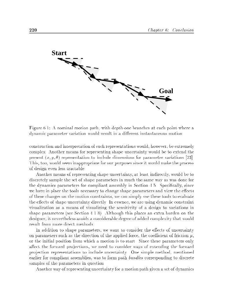
�� Chapter � Conclusion
Start
Goal
Figure ���� A nominal motion path� with depth�one branches at each point where adynamic parameter variation would result in a di�erent instantaneous motion�
construction and interpretation of such representations would� however� be extremelycomplex� Another means for representing shape uncertainty would be to extend thepresent �x� y� �� representation to include dimensions for parameter variations �����This� too� would seem inappropriate for our purposes since it would make the processof design even less tractable�
Another means of representing shape uncertainty� at least indirectly� would be todiscretely sample the set of shape parameters in much the same way as was done forthe dynamics parameters for compliant assembly in Section ��� Speci�cally� sincewe have in place the tools necessary to change shape parameters and view the e�ectsof these changes on the motion constraints� we can simply use these tools to evaluatethe e�ects of shape uncertainty directly� In essence� we are using dynamic constraintvisualization as a means of visualizing the sensitivity of a design to variations inshape parameters �see Section ������ Although this places an extra burden on thedesigner� it nevertheless avoids a considerable degree of added complexity that wouldresult from more direct methods�
In addition to shape parameters� we want to consider the e�ects of uncertaintyon parameters such as the direction of the applied force� the coe�cient of friction ��or the initial position from which a motion is to start� Since these parameters onlya�ect the forward projections� we need to consider ways of extending the forwardprojection representations to include uncertainty� One simple method� mentionedearlier for compliant assemblies� was to form path bundles corresponding to discretesamples of the parameters in question�
Another way of representing uncertainty for a motion path given a set of dynamics
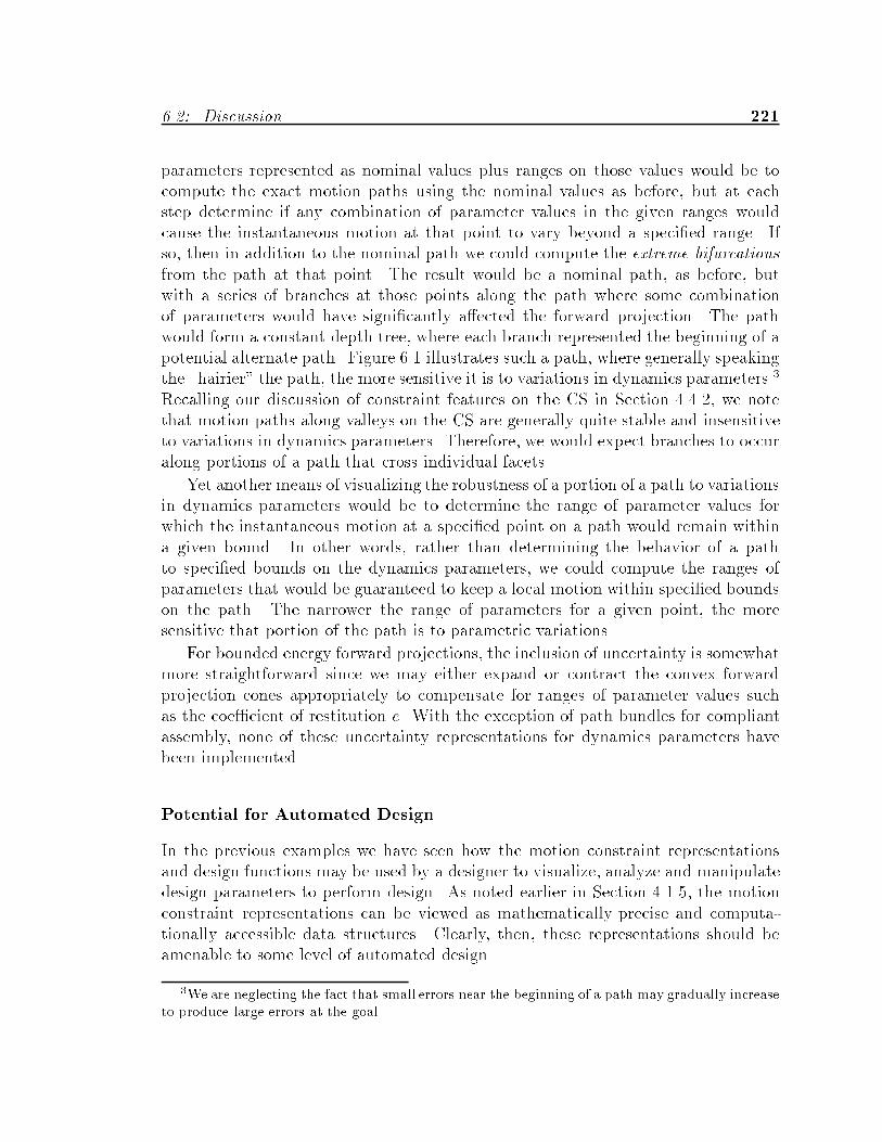
��� Discussion ���
parameters represented as nominal values plus ranges on those values would be tocompute the exact motion paths using the nominal values as before� but at eachstep determine if any combination of parameter values in the given ranges wouldcause the instantaneous motion at that point to vary beyond a speci�ed range� Ifso� then in addition to the nominal path we could compute the extreme bifurcationsfrom the path at that point� The result would be a nominal path� as before� butwith a series of branches at those points along the path where some combinationof parameters would have signi�cantly a�ected the forward projection� The pathwould form a constant depth tree� where each branch represented the beginning of apotential alternate path� Figure ��� illustrates such a path� where generally speakingthe �hairier� the path� the more sensitive it is to variations in dynamics parameters��
Recalling our discussion of constraint features on the CS in Section ���� we notethat motion paths along valleys on the CS are generally quite stable and insensitiveto variations in dynamics parameters� Therefore� we would expect branches to occuralong portions of a path that cross individual facets�
Yet another means of visualizing the robustness of a portion of a path to variationsin dynamics parameters would be to determine the range of parameter values forwhich the instantaneous motion at a speci�ed point on a path would remain withina given bound� In other words� rather than determining the behavior of a pathto speci�ed bounds on the dynamics parameters� we could compute the ranges ofparameters that would be guaranteed to keep a local motion within speci�ed boundson the path� The narrower the range of parameters for a given point� the moresensitive that portion of the path is to parametric variations�
For bounded energy forward projections� the inclusion of uncertainty is somewhatmore straightforward since we may either expand or contract the convex forwardprojection cones appropriately to compensate for ranges of parameter values suchas the coe�cient of restitution e� With the exception of path bundles for compliantassembly� none of these uncertainty representations for dynamics parameters havebeen implemented�
Potential for Automated Design
In the previous examples we have seen how the motion constraint representationsand design functions may be used by a designer to visualize� analyze and manipulatedesign parameters to perform design� As noted earlier in Section ����� the motionconstraint representations can be viewed as mathematically precise and computa�tionally accessible data structures� Clearly� then� these representations should beamenable to some level of automated design�
�We are neglecting the fact that small errors near the beginning of a path may gradually increaseto produce large errors at the goal�

��� Chapter � Conclusion
What we have also seen in the previous examples is a high degree of very non�linear coupling between parameter modi�cations and changes to motion constraints�particularly for the motion constraints found in the vibratory bowl feeder examples�What algorithms might have a reasonable chance of success for such a domain� Twoparadigms that come to mind are�
� Iterative generate and test� Perhaps the simplest approach to automateddesign would be the semi�random perturbation of design variables coupled witha binary go�no�go �lter on the resulting designs�
� Non�linear optimization� Another option would be to compute and imposesome form of appropriate metric on the motion constraint representations �andby means of apparent�inversion on the underlying design variables� that wouldbe maximized or minimized�
The �rst approach has the obvious appeal of simplicity� One serendipitous ad�vantage of having to implement the motion constraint representations for use ininteractive design is the fact that they may be computed quickly� For example� be�cause we can compute the full set of motion constraints for a typical feeder example�including forward projections� on the order of once per second� it is not unreason�able to assume that a random search of the design space might yield viable designswithin a reasonable time frame� The resolution at which we randomly sample willbe a particularly important consideration since we do not know how tightly groupedpotential designs may be� Of course� all of this assumes that the space of designs isrelatively small and viable designs are not too sparsely scattered� which in generalmay not be the case�
The second approach requires us to construct an additional metric that char�acterizes� preferably in a continuous sense� a good design� For bowl feeders we areprimarily concerned with manipulating the proximity of motion paths to unsupportedregions on the CS� Speci�cally� given a desired accept path� our goal is to both� a�maximize the distance between all points on the accept path and all unsupportedregions on the CS surface� and b� minimize the distance between points on all rejectpaths and support transition boundaries� In case b�� we ideally want the distancesto go to zero� i�e� rejected motions should intersect unsupported regions� Using thisdescription� we could envision a cost function metric based on proximity betweenpaths and unsupported regions in the form of a potential energy function� In thisscenario� as the design parameters were varied so as to minimize the cost function�the unsupported regions would act as sources to repel the accept path and at thesame time act as sinks to attract the remaining reject paths�
A design algorithm based on standard linear optimization techniques using sucha cost function� although appealing� would possess some major drawbacks as well�Perhaps the most serious of these is the fact that� due to the inherent complexity

��� Discussion ���
of the motion constraints and the nonlinear coupling between variations to the con�straints and parameters� there would likely be a number of local minima that wouldnot necessarily correspond to satisfactory design solutions� Therefore� a simple hillclimbing algorithm would be unlikely to produce many good designs� Furthermore�there is no guarantee on the stability of or convergence toward a design goal of suchan algorithm�
One potential solution is suggested by examining the feeder design methodologyoutlined by the �owchart in Figure ��� that was intended for use by a humandesigner� Speci�cally� the nested iterative design loops� each working at a lower levelof detail on a smaller subset of design parameters� suggests that local optimizationof constraints coupled with an occasional reformulation of the higher level problem�or large scale jump in design space� could yield better results than local optimizationalone� Therefore� an automated optimization algorithm based on simulated annealingor similar strategies may provide the best compromise�
We could utilize a number of simpli�cations and optimizations by taking advan�tage of the structure of the motion constraint representations� For example� ratherthan constructing one complex energy function we may be able to formulate a numberof simpler energy metrics based on local proximity between selected points on eachpath and selected points on nearby support transition boundaries that would allow alinear optimization strategy to quickly converge to local minima� These local energymetrics would have to be recomputed for each signi�cant change in the topologyof the motion constraint representations� which would occur more or less frequentlydepending on the current annealing temperature� We could also take advantage ofthe coupling sensitivity information available from the implemented design functionsto compute local gradients in the design space to help determine in which directionlarger scale parametric changes might be more likely to achieve a desired design�Once again� we cannot guarantee that such an algorithm would converge to a suit�able design� Nor can we say anything de�nite about the rate of convergence of suchan optimization strategy�
Finally� what about automated design algorithms for compliant assembly� Asin the case of interactive design� the set of constraints that must be manipulatedis smaller and less tightly coupled than for bowl feeders� A brute force generateand test design paradigm might therefore be better suited to assembly since we areworking over a smaller range of motion constraints� An energy based optimiza�tion metric similar to the one described above in which the assembly goal acts as asink would also appear to be a reasonable strategy to investigate� One complicat�ing factor� as mentioned earlier in Section ��� is that the addition of non�assemblyconstraints would seem to be an important consideration since unconstrained auto�mated algorithms that only optimize on the basis of motion constraints would tendto turn everything into a pair nesting cones with the compliant center at the mov�ing part�s tip� Labeling certain object features as �xed would presumably maintain
��� Chapter � Conclusion
non�assembly constraints� but leaving these potentially over�conservative constraints�untouchable� by the algorithm could often result in no satisfactory solutions beingfound�
Many of the above issues� as well as working implementations of automated designstrategies along the lines of those described above� remain issues for further research�
��� Future Work
Near Term
The limitations of the present implementation of cspace�shell suggest some nearerterm enhancements that could improve the power and usefulness of the representa�tions and tools� Additional enhancements and extensions might include the following�
� Complete the development and implementation of the energy bounded forwardprojections necessary to model the jig and APOS feeder application domains�The main challenge here is the fact that implementing these forward projectionswould require us to extend the current incremental CS topology construction tocompute a more complete representation of the global CS topology� similar tothe approach used by Brost ����� Since this computation would almost certainlyrequire more time� we would most likely have to adopt the present approachof computing CS topology only as a post�processing step after an interactiveshape modi�cation operation has been completed�
� Implement the superposition of motion constraints generated for planar poly�gons representing multiple slices of three dimensional objects taken at di�erentz�heights�
� Expand upon the quasi�static dynamics model for exact motion integration toinclude dynamic e�ects due to inertia� Depending on the operating conditionsfor the bowl feeder and assembly application domains� more detailed dynamicmodels may improve the simulation and veri�cation of object motions�
Longer Term
All of the above implementational enhancements� along with most of those listedin the previous section� are well within the scope of the existing representationsand algorithms� We might view them as features that we should have known toimplement� or approaches that we should have adopted earlier on in the research�
Other enhancements are su�ciently di�erent or challenging to be classi�ed assigni�cant new research directions based on the current work� Some of these include�
��� Future Work ���
� Implement the design functions necessary to allow direct manipulation of mo�tion paths vs� motion constraints as discussed in the previous section�
� Develop and implement representations for uncertainty and reliability in thedesign of motion constraints along the lines of those outlined in Section ������
� Develop and implement automated and semi�automated design techniques alongthe lines of those discussed in Section ������
� Explore other application domains beyond the four developed in Chapter ��and extend the representations and tools as necessary� Examples of poten�tially promising domains include the design of tools and fasteners as illustratedin Chapter �� electrical connectors and couplings� multiple degree of freedommechanisms� ���
� Expand and integrate the motion constraint representations with other engi�neering representations and analysis�design techniques such as� analytic andnumerical models of cost� material strength and sti�ness� dynamics and vibra�tion� and manufacturing processes such as machining and casting� Examplesfrom the domain of assembly examined in Section �� clearly illustrated theneed for such models�
� A considerably more challenging extension than the superposition of multipleplanar slices of a �D object would be to model three dimensional objects directlyas polyhedra� and compute the motion constraints for interactions among thosepolyhedra constrained to move in �x� y� ��� Type A and type B facets wouldcorrespond to face�vertex and vertex�face interactions between the moving andstationary polyhedra� respectively� and a new facet type representing edge�edgeinteractions �type C� would also be required �see Lozano�P erez �����
� Beyond polyhedra� a signi�cant challenge would be to generate and render mo�tion constraints produced by more general shape interactions� such as objectsmodeled using bi�cubic patches�
� Finally� we should by no means by committed to the motion constraint repre�sentation or interactive design environment if another representation appearsto hold more promise in simplifying the tasks of analysis and design� Forexample� it may be possible to develop hybrid functional metaphor�motionconstraint representations that could ease the designer�s burden of learningnew and unfamiliar representations�

��� Appendices

Energy Bounded Forward
Projections
Appendix A
A�� Forward Projections for Dropped Objects
This section derives the models used to compute the forward projection of a droppedparticle for single and double impacts with oriented surfaces in a gravity �eld�
Single Bounce
The pro�le for the maximum height reached after the initial bounce of a particle�hmax� in Figure �� � as a function of the impact surface orientation �� is derived as
h0
hmax 1
hmax 2
ϕ1 ϕ2 = f (ϕ1)
g
y
x
v2
v1v2
v3
Figure A��� Model of single and double impacts for a dropped particle�
��

��� Appendix A� Energy Bounded Forward Projections
follows�
The pre�impact velocity v of the particle is given by conservation of energy� assumingzero initial velocity� as�
�
�mv� " mgh�
so thatv "
q�gh�
As a conservative approximation� we assume the surface to be frictionless� We thencompute the post�impact velocity components using the coe�cient of restitution eand equation ����
v�x " v�� � e� sin�� cos��
v�y " v�ecos��� � sin�����
The post�impact motion of the particle is parabolic�
x�t� " x � v�xt
y�t� " y � v�yt� g
�t��
Finally� at the point of maximum height we have�
tymax "v�yg
xymax " x � v�xtymax " x �v�g
��� � e� sin�� cos���ecos
��� � sin�����
ymax " y �v��y�g
" y �v��g
�ecos��� � sin���
���
Double Bounce
The pro�le for the maximum height reached after the second bounce of a particle�hmax� in Figure �� � as a function of the impact surface orientation �� is derived asfollows�
Assuming the height of the second point of impact is the same as the �rst��
v�x " v�x " v�� � e� sin�� cos��
�The equations for the case where the second impact is at a di�erent height from the �rst areconsiderably more complex but the solutions indicate that the forward projection derived from theequal height analysis given here contains the other paths�

A��� Forward Projections for Dropped Objects ���
v�y " �v�y " �v�ecos��� � sin�����
and
jv�j " jv�j " v
qsin� �� � e� cos� ���
We require the velocity after the second impact to be vertical so that
v�x " �
From this constraint and from the symmetry of the problem we have the followingrelationship between �� and ���
�� � tan����
etan��
�" tan��
��
etan��
�� ��
We may solve the resulting expression numerically to achieve�
�� " f����
We may now perform the same pre and post�impact analysis as was don for the �rstbounce� The result is
v�y " jv�j " v� �sin� sin�� � e cos� cos���
where
� " tan���e tan���
After rearranging we have
v� " v�e cos�
cos��
where
jv�j "q�gh sin
� �� � e� cos� ��
Finally� from conservation of energy we have
hmax� "v���g
where� from above� v� " g�����

�� Appendix A� Energy Bounded Forward Projections
A�� Non�Conservative Bouncing
In this section we estimate the maximumheight attainable by a particle starting fromrest on a table with coe�cient of restitution e� and vibrating with frequency �t andamplitude A� We compute the maximum height by considering the most extremeof impact conditions� Speci�cally� we assume that after falling from the maximumheight� the energy lost by the particle during impact with the table exactly balancesthe maximum energy imparted to the particle by the table �i�e� when the table ismoving at its maximum upward velocity��
From equation ��� we have�
vtable � v� " �e�v� � vtable�
where v� and v� are the pre and post�impact velocities of the particle� respectively�
From an energy balance on the particle under the above assumptions we have�
v� " v�
So that the maximum post�impact velocity of the particle is
vparticlemax "�� � e�
�� � e�vtable�
The maximum velocity of the table is
vtablemax " A��
From conservation of energy after the particle leaves the table�
Hmax "v�particlemax
�g
so that �nally we have
Hmax "�A��
�
�g
�� � e��
��� e���

Facet Curvature
Appendix B
In this appendix we derive the maximum motion integration stepsize based on aspeci�ed upper error bound Emax�
We begin with a derivation of the general curvature �n along a �D surface from Faux� Pratt ���� The surface is de�ned as a vector quantity r where
r " xi� yj � zk
A curve on a �u� v� surface is given by u " u�t� and v " v�t� where t is a parameteralong the curve� The surface normal at a given point on the surface is given in termsof the parameters �u� v� by
n "
���r�u� ��r
�v
� ��r�u� ��r
�v
�
The curvature �n of the surface along the curve is given by
�n ")uTD )u
)uTG )u
where
u " �u�t�� v�t��T �
and D is the second fundamental matrix given by
D "
�n � ���r
�u�n � ���r
�u�v
n � ���r�v�u
n � ���r�v�
�
���
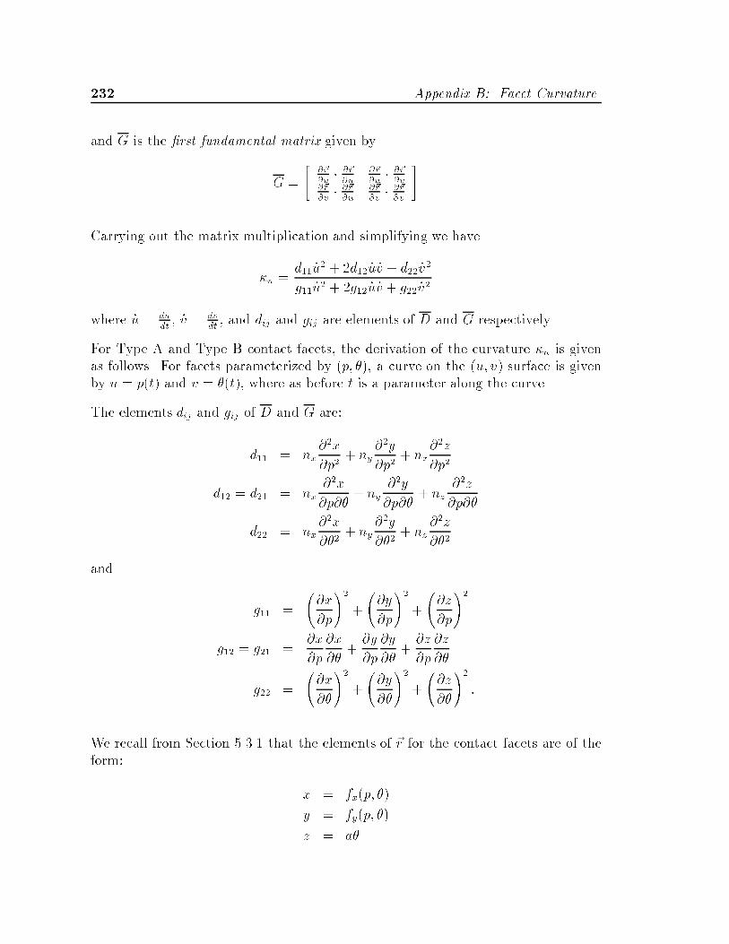
��� Appendix B� Facet Curvature
and G is the �rst fundamental matrix given by
G "
���r�u� ��r�u
��r�u� ��r�v
��r�v� ��r�u
��r�v� ��r�v
�
Carrying out the matrix multiplication and simplifying we have
�n "d�� )u� � �d�� )u )v � d�� )v�
g�� )u� � �g�� )u )v � g�� )v�
where )u " dudt� )v " dv
dt� and dij and gij are elements of D and G respectively�
For Type A and Type B contact facets� the derivation of the curvature �n is givenas follows� For facets parameterized by �p� ��� a curve on the �u� v� surface is givenby u " p�t� and v " ��t�� where as before t is a parameter along the curve�
The elements dij and gij of D and G are�
d�� " nx��x
�p�� ny
��y
�p�� nz
��z
�p�
d�� " d�� " nx��x
�p��� ny
��y
�p��� nz
��z
�p��
d�� " nx��x
���� ny
��y
���� nz
��z
���
and
g�� "
��x
�p
��
�
��y
�p
��
�
��z
�p
��
g�� " g�� "�x
�p
�x
����y
�p
�y
����z
�p
�z
��
g�� "
��x
��
��
�
��y
��
��
�
��z
��
��
�
We recall from Section ����� that the elements of r for the contact facets are of theform�
x " fx�p� ��
y " fy�p� ��
z " a�
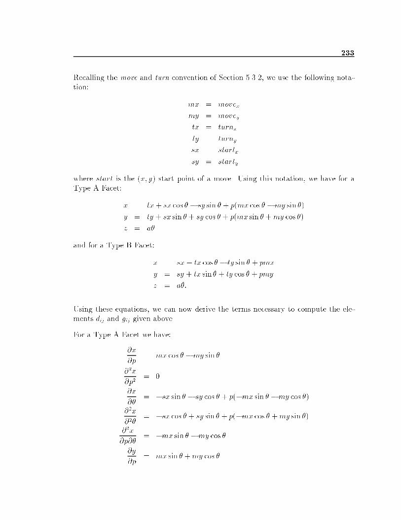
���
Recalling the move and turn convention of Section ������ we use the following nota�tion�
mx " movex
my " movey
tx " turnx
ty " turny
sx " startx
sy " starty
where start is the �x� y� start point of a move� Using this notation� we have for aType A Facet�
x " tx� sx cos � � sy sin � � p�mx cos � �my sin ��
y " ty � sx sin � � sy cos � � p�mx sin � �my cos ��
z " a�
and for a Type B Facet�
x " sx� tx cos � � ty sin � � pmx
y " sy � tx sin � � ty cos � � pmy
z " a��
Using these equations� we can now derive the terms necessary to compute the ele�ments dij and gij given above�
For a Type A Facet we have�
�x
�p" mx cos � �my sin �
��x
�p�"
�x
��" �sx sin � � sy cos � � p��mx sin � �my cos ��
��x
���" �sx cos � � sy sin � � p��mx cos � �my sin ��
��x
�p��" �mx sin � �my cos �
�y
�p" mx sin � �my cos �

��� Appendix B� Facet Curvature
��y
�p�"
�y
��" sx cos � � sy sin � � p�mx cos � �my sin ��
��y
���" �sx sin � � sy cos � � p��mx sin � �my cos ��
��y
�p��" mx cos � �my sin ��
�z
�p"
��z
�p�"
�z
��" a
��z
���"
��z
�p��" �
For a Type B Facet we have�
�x
�p" mx
��x
�p�"
�x
��" �tx sin � � ty cos �
��x
���" �tx cos � � ty sin �
��x
�p��"
�y
�p" my
��y
�p�"
�y
��" tx cos � � ty sin �
��y
���" �tx sin � � ty cos �

���
��y
�p��"
�z
�p"
��z
�p�"
�z
��" a
��z
���"
��z
�p��" �
In Section ���� we developed the expressions needed to compute the instantaneousdirection of motion on a facet surface� in terms of (p and (�� from the net force com�ponents at the point of contact� Using Equations ��� and ��� we can approximate)u and )v as�
)u "dp
dt� (P
(T"
(Pp(P � �(��
)v "d�
dt� (�
(T"
(�p(P � �(��
�
Using this approximation for )u and )v� and the elements dij and gij computed fromthe above expressions for the appropriate facet type� we compute the facet curvature�n along the speci�ed �(p�(�� direction of motion across the facet� From the facetcurvature� we compute the equivalent radius of curvature R as
R "�
�n�
Figure B�� shows the relationship between a speci�ed maximum error Emax� theradius of curvature R along the motion path� and the maximum stepsize (Tmax�From the �gure we see that
(Tmax " R sin �max
andEmax " R�� � cos���
With some simple trigonometry and rearranging we have
cos �max " � � E
R

��� Appendix B� Facet Curvature
t
ncs
Emax
Tmax
Facet Curve
R
ϕ
Figure B��� Determining the maximum integration stepsize on a curved facet�
and
sin�max "q�� cos� �max
"
s��
�� � E
R
��
"�
R
p�ER � E��
Finally we have
(Tmax " R sin�max "q�EmaxR �E�
max
"
s�Emax
�n� E�
max
Given (Tmax� we can compute the maximum stepsize in terms of the facet parame�ters �p� �� using Equations ��� and ��� in Section ����� which we repeat here forreference
(Pmax "
�(pp
(p� �(��
�(Tmax
(�max "
�(�p
(p� �(��
�(Tmax�
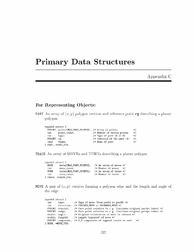
Primary Data Structures
Appendix C
For Representing Objects�
PART An array of �x� y� polygon vertices and reference point cg describing a planarpolygon�
typedef struct �
PPOINT points�MAX�PART�POINTS�� �� Array of points ��
int point�count� �� Number of vertex points ��
int type� �� Type of part �A or B ��
PPOINT cg� �� Centroid of the part �A ��
char �name� �� Name of part ��
PART� �PART�PTR�
TRACE An array of MOVEs and TURNs describing a planar polygon�
typedef struct �
MOVE moves�MAX�PART�POINTS�� �� An array of moves ��
int move�count� �� Number of moves ��
TURN turns�MAX�PART�POINTS�� �� An array of turns ��
int turn�count� �� Number of turns ��
TRACE� �TRACE�PTR�
MOVE A pair of �x� y� vertices forming a polygon edge and the length and angle ofthe edge�
typedef struct �
int type� �� Type of move �from partA or partB ��
int direction� �� FORWARD�MOVE or BACKWARD�MOVE ��
PPOINT startpt� �� Part point relative to c�g� �Includes original partpt index ��
PPOINT endpt� �� Part point relative to c�g� �Includes original partpt index ��
double angle� �� Original orientation of move in radians ��
double length � �� Length �squared of move ��
PPOINT component� �� X�Y components of segment �start to end ��
MOVE� �MOVE�PTR�
��

��� Appendix C� Primary Data Structures
TURN An �x� y� vertex point� with angles for the entering edge and exiting polygonedge� and a LEFT TURN or RIGHT TURN corresponding to a convex orconcave vertex�
typedef struct �
int type� �� Type of turn �from partA or partB ��
int direction� �� LEFT�TURN or RIGHT�TURN ��
PPOINT turnpt� �� Part point relative to c�g� �Includes original partpt index ��
double start�angle� �� Original orientation of move entering turn in radians ��
double end�angle� �� Original orientation of move leaving turn in radians ��
TURN� �TURN�PTR�
For Representing Motion Constraints�
CS An array of �NM type A and type B contact facets�
typedef struct �
FACET facetsA�MAX�MOVES��MAX�TURNS�� �� FACET array � D indexed by MOVE and TURN ��
int facetsA�moves� �� Number of facetsA moves �partA moves ��
int facetsA�turns� �� Number of facetsA turns �partB turns ��
FACET facetsB�MAX�MOVES��MAX�TURNS�� �� FACET array � D indexed by MOVE and TURN ��
int facetsB�moves� �� Number of facetsB moves �partB moves ��
int facetsB�turns� �� Number of facetsB turns �partA turns ��
CS� �CS�PTR�
FACET Contains information on facet type and size for rendering a contact facet�arrays of REL�FACETs containing adjacent and intersecting facets for computingmotion paths� and a support map to record the support status of points on thefacet surface�
typedef struct �
int type� �� Type of FACET �TYPE�A or TYPE�B ��
int direction� �� FORWARD�MOVE or BACKWARD�MOVE facet ��
int move�index� �� Index to part MOVE forming this facet ��
MOVE�PTR move� �� Pointer to MOVE forming this facet �for speed ��
int turn�index� �� Index to part TURN forming this facet ��
TURN�PTR turn� �� Pointer to TURN forming this facet �for speed ��
double min�theta� �� Minimum theta for which this facet is valid ��
double max�theta� �� Maximum theta for which this facet is valid ��
int adjacents�posted� �� Flag indicating if adjacents have been posted ��
REL�FACET�PTR adjacents� �� BEGINNING of the array of adjacents ��
int adjacents�count� �� Number of adjacent facets ��
int intersects�posted� �� Flag indicating if intersects have been posted ��
REL�FACET�PTR intersects� �� BEGINNING of the array of intersects ��
int intersects�count� �� Number of intersecting facets ��
int support�status� �� �SUPPORTED� UNSUPPORTED� TEST�SUPPORT ��
SUPPORT�PTR support�map� �� Beginning of array of support transitions ��
int support�map�count� �� Number of support�map elements ��
double support�delta�theta� �� Theta step at which support map is computed ��
double support�delta�p� �� Nominal p step at which support map is computed ��
FACET� �FACET�PTR�
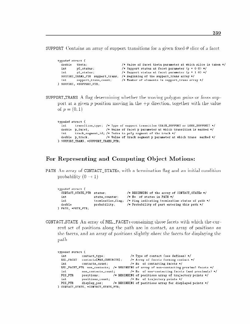
���
SUPPORT Contains an array of support transitions for a given �xed�� slice of a facet�
typedef struct �
double theta� �� Value of facet theta parameter at which slice is taken ��
int p��status� �� Support status at facet parameter �p � ��� ��
int p��status� �� Support status at facet parameter �p � ��� ��
SUPPORT�TRANS�PTR support�trans� �� Beginning of the support�trans array ��
int support�trans�count� �� Number of elements in support�trans array ��
SUPPORT� �SUPPORT�PTR�
SUPPORT TRANS A �ag determining whether the moving polygon gains or loses sup�port at a given p position moving in the �p direction� together with the valueof p " �� ���
typedef struct �
int transition�type� �� Type of support transition �GAIN�SUPPORT or LOSE�SUPPORT ��
double p�facet� �� Value of facet p parameter at which transition is marked ��
int track�segment�id� �� Index to poly segment of the track ��
double p�track� �� Value of track segment p parameter at which trans� marked ��
SUPPORT�TRANS� �SUPPORT�TRANS�PTR�
For Representing and Computing Object Motions�
PATH An array of CONTACT�STATEs� with a termination �ag and an initial conditionprobability �� ��
typedef struct �
CONTACT�STATE�PTR states� �� BEGINNING of the array of CONTACT�STATEs ��
int state�counter� �� No� of states in PATH ��
int termination�flag� �� Flag indicating termination status of path ��
double probability� �� Probability of part entering this path ��
PATH� �PATH�PTR�
CONTACT STATE An array of REL�FACETs containing those facets with which the cur�rent set of positions along the path are in contact� an array of positions onthe facets� and an array of positions slightly above the facets for displaying thepath�
typedef struct �
int contact�type� �� Type of contact �see defines ��
REL�FACET contacts�MAX�CONTACTS�� �� Array of facets forming contact ��
int contacts�count� �� No� of contacting facets ��
REL�FACET�PTR non�contacts� �� BEGINNING of array of non�contacting proximal facets ��
int non�contacts�count� �� No� of non�contacting facets �and proximals ��
POS�PTR positions� �� BEGINNING of positions array of trajectory points ��
int positions�count� �� No� of trajectory points ��
POS�PTR display�pos� �� BEGINNING of positions array for displayed points ��
CONTACT�STATE� �CONTACT�STATE�PTR�

�� Appendix C� Primary Data Structures
FACET FORCE STATE A record of the instantaneous net force state on a single facet ata point along the path� including the position� normal and tangential vectors�and vectors bounding the con�guration space friction cone�
typedef struct �
FACET�PTR facet� �� Pointer to a FACET ��
POS�PTR pos� �� Pointer to POS on facet ��
double p� �� Param� P corresponding to pos on FACET ��
double n�co���� �� CS normal at point ��
double m�p���� �� CS m�p at point ��
double m�theta���� �� CS m�theta at point ��
double n�fc���� �� Normal to CS friction cone plane ��
double f�rhs���� �� RHS bounding ray of CS friction cone ��
double f�lhs���� �� LHS bounding ray of CS friction cone ��
double f�net���� �� Net force on contact ��
FACET�FORCE�STATE� �FACET�FORCE�STATE�PTR�
PROXIMAL The signed distance of a point from the surface of a non�contacting facetmeasured in a constant�� plane�
typedef struct �
int proximal�state� �� State of facet adjacency or point�to�line proximity ��
double distance� �� Signed distance from point�to�line ��
PROXIMAL� �PROXIMAL�PTR�
MOTION PARAMS A record of the external force applied to the reference point� thepath integration step size� and parameters and ��
typedef struct �
double f�ext���� �� Externally applied force ��
double max�step� �� Maximum step size for integration ��
double rho� �� Radius of gyration� scales theta to X�Y ��
double mu� �� Coefficient of friction ��
MOTION�PARAMS� �MOTION�PARAMS�PTR�

Bibliography
��� H� Asada� A� B� By� �Kinematics of Workpart Fixturing�� IEEE Interna�tional Conference on Robotics and Automation� March ����� pp� �� ����
��� I� I� Artobolevsky� Mechanisms in Modern Engineering Design� MIR Pub�lishers� Moscow� �� ��
��� F� Avinaim� J� D� Boissonnat� B� Faverjon� �A Practical Exact MotionPlanning Algorithm for Polygonal Objects Amidst Polygonal Obstacles�� IEEEInternational Conference on Robotics and Automation� April ����� pp� ����������
�� C� Bajaj� M� Kim� �Generation of Con�guration Space Obstacles� The Caseof Moving Algebraic Curves�� International Conference on Robotics and Au�tomation� Raleigh� NC� April ��� � pp� � �����
��� J� J� Bausch� K� Youcef�Toumi� �Kinematic Methods for Automated Fix�ture Recon�guration Planning�� International Conference on Robotics and Au�tomation� May ���� pp� ��������
��� R� M� C� Bodduluri� J� M� McCarthy� �Design of Spatial MechanismsUsing Constraint Manifolds�� Department of Mechanical Engineering� U� C�Irvine� February �����
� � G� Boothroyd� C� Poli� L� Murch� Automatic Assembly� Marcel Dekker�New York� �����
��� G� Boothroyd� P� Dewhurst� Design for Assembly � ADesigners Handbook� Department of Mechanical Engineering� University ofMassachusetts� Amherst� Mass�� �����
��
��� BIBLIOGRAPHY
��� D� A� Bourne� D� Navinchandra� R� Ramaswamy� �Relating Tolerancesand Kinematic Behavior�� The Robotics Institute� Carnegie Mellon University�Technical Report CMU�RI�TR������ April �����
��� W� E� Boyes� Ed�� Jigs and Fixtures� �nd� Edition� Society of ManufacturingEngineers� Dearborn� MI� �����
���� M� S� Branicky� W� S� Newman� �Rapid Computation of Con�gurationSpace Obstacles�� IEEE International Conference on Robotics and Automa�tion� Cincinnati� OH� May ���� pp� �����
���� R� C� Brost� �Dynamic Analysis of Planar Manipulation Tasks�� IEEE In�ternational Conference on Robotics and Automation� Nice� France� May �����pp� �� �����
���� R� C� Brost� �Analysis and Planning of Planar Manipulation Tasks�� PhDThesis� CMU�CS������� Carnegie Mellon University� January �����
��� S� J� Buckley� �Planning and Teaching Compliant Motion Strategies�� Arti��cial Intelligence Laboratory� Massachusetts Institute of Technology� TechnicalReport ���� January ��� �
���� M� E� Caine� T� Lozano�P�erez� W� P� Seering� �Assembly Strategies forChamferless Parts�� IEEE International Conference on Robotics and Automa�tion� Scottsdale� AZ� May ����� pp� �� �
���� M� Caine� �The E�ect of Part Shape on Planar Insertion Operations��Proceedings of the Second ASME Conference on Flexible Assembly Systems�Chicago� IL� Sept� ���� pp� ��������
�� � M� E� Caine� �The Design of Shape from Motion Constraints�� PhD Thesis�Department of Mechanical Engineering� Massachusetts Institute of Technology�January �����
���� J� F� Canny� The Complexity of Robot Motion Planning� MIT Press� Cam�bridge� MA� �����
���� A� Christian� Personal Communication� November� ����
��� M� S� Darlow� D� M� Avidar� M� W� Steiner� �A Procedure for Compar�ative Evaluation of Design for Assembly Methodologies�� ASME Advances inDesign Automation������ DE�Vol� ���� ��� � pp� ������
���� T� L� De Fazio� et� al�� �A Prototype for Feature�Based Design for As�sembly � Revision ��� CSDL�P���� � The Charles Stark Draper Laboratory�Cambridge� MA� ����
BIBLIOGRAPHY ���
���� B� R� Donald� �Motion Planning with Six Degrees of Freedom�� Arti�cialIntelligence Laboratory� TR� ��� Massachusetts Institute of Technology� June����
���� B� R� Donald� �Error Detection and Recovery for Robot Motion Planningwith Uncertainty�� Arti�cial Intelligence Laboratory� Massachusetts Instituteof Technology� Technical Report ���� July ��� �
��� B� Donald� D� Pai� �On The Motion of Compliantly�Connected Rigid Bodiesin Contact� Part II� A System for Analyzing Designs for Assembly�� IEEEInternational Conference on Robotics and Automation� Cincinnati� OH� May���� pp� � ���� ���
���� The Charles Stark Draper Laboratory� Third Annual Seminar on Ad�vanced Assembly Automation� Nov� ����� pp� ��c������c����
���� M� A� Erdmann� �On Motion Planning with Uncertainty�� Arti�cial Intel�ligence Laboratory� Massachusetts Institute of Technology� Technical Report��� May ����
�� � M� A� Erdmann� M� T� Mason� �An Exploration of Sensorless Manipu�lation�� IEEE Journal of Robotics and Automation� Vol� � No� � ����� pp������ ��
���� M� A� Erdmann� �On Probabalistic Strategies for Robot Tasks�� Arti�cialIntelligence Laboratory� Massachusetts Institute of Technology� Technical Re�port ����� March ����
���� B� Faltings� �Qualitative Place Vocabularies for Mechanisms in Con�gurationSpace�� PhD Thesis� Report No� UIUCDCS�R�� ����� University of Illinois�July ��� �
��� I� D� Faux� M� J� Pratt� Computational Geometry for Design andManufacture� John Wiley � Sons� New York� �� ��
���� J� Foley� et� al� Computer Graphics � Principles and Practice� �nd� Edition�Addison�Wesley� Reading� MA� ����
���� T� Fujimori� �Development of Flexible Assembly System Smart�� Proc� Int�Symposium on Industrial Robotics� October ���� pp� �����
���� B� J� Gilmore� D� A� Streit� �A Rule�Based Algorithm to Predict the Dy�namic Behavior of Mechanical Part Orienting Operations�� IEEE InternationalConference on Robotics and Automation� Philadelphia� PA� ����� pp� ���������
��� BIBLIOGRAPHY
��� K� Y� Goldberg� �Stochastic Plans for Robotic Manipulation�� PhD Thesis�CMU�CS������� Carnegie Mellon University� August ����
���� S� J� Gordon� �Automated Assembly Using Feature Localization�� Arti��cial Intelligence Laboratory� Massachusetts Institute of Technology� TechnicalReport ���� December �����
���� J� Guckenheimer� P� Holmes� Nonlinear Oscillations� Dynamical Sys�tems� and Bifurcations of Vector Fields� Third Printing� Springer�Verlag� NewYork� �����
�� � L� Guibas� L� Ramshaw� J� Stol � �A Kinetic Framework for Computa�tional Geometry�� Proceedings of the �th Annual IEEE Conference on theFoundations of Computer Science� Tuscon� AZ� ����� pp� ������
���� R� Gupta� M� J� Jakiela� �Qualitative Simulation of Kinematic Pairs viaSmall�Scale Interference Detection�� ASME Fourth International Conferenceon Design Theory and Methodology� Scottsdale� AZ� September �����
���� D� A� Hoeltzel� W� H� Chieng� �Pattern Matching Synthesis as an Auto�mated Approach to MechanismDesign�� Proceedings of the ���� ASME DesignTechnical Conferences � �th Design Automation Conference� DE�Vol� �����Montreal� Quebec� Canada� Sept� ����� pp� ������
�� S� Goyal� �Planar Sliding of a Rigid Body with Dry Friction� Limit Surfacesand Dynamics of Motion�� PhD Thesis� Dept� of Mechanical Engineering� Cor�nell University� January �����
��� Inoue� Hirochika� �Force Feedback in Precise Assembly Tasks�� Arti�cialIntelligence Laboratory� Massachusetts Institute of Technology� AI Memo����Aug� �� �Reprinted in Winston� P� H�� and Brown� R� H�� eds�� Arti�cialIntelligence� An MIT Perspective� MIT Press� �� ���
��� M� J� Jakiela� P� Y� Papalambros� �Design and Implementation of anIntelligent CAD System�� ASME Advances in Design Automation������ DE�Vol� ���� ��� � pp� �������
��� L� Joskowicz� S� Addanki� �Innovative Shape Design� A Con�gurationSpace Approach��Courant Institute of Mathematical Sciences� New York Uni�versity� Technical Report ���� March �����
�� L� Joskowcz� �Reasoning about Shape and Kinematic Function in Mechan�ical Devices�� PhD Thesis� Technical Report No� �� New York University�September �����

BIBLIOGRAPHY ���
��� L� Joskowicz� E� Sachs� �Unifying Kinematics and Dynamics for the Auto�matic Analysis of Machines�� IBM Technical Report RC ��� �� March ����
��� M� Juodate� A� Saito� Personal Communication� August� ����
� � G� A� Kramer� Solving Geometric Constraint Systems� A Case Studyin Kinematics� MIT Press� Cambridge� MA� �����
��� J� Lengyel� M� Reichert� B� R� Donald� and D� P� Greenberg� �Real�Time Robot Motion Planning Using Rasterizing Computer Graphics Hard�ware�� Proceedings of SIGGRAPH ��� Dallas� TX� August ����
��� T� Lozano�P�erez� �Spatial Planning� A Con�guration Space Approach��IEEE Transactions on Computers� Vol� C���� No� �� Feb� ����� pp� ������
��� T� Lozano�P�erez� M� T� Mason� R� H� Taylor� �Automatic Synthesis ofFine�Motion Strategies for Robots�� Proceedings� International Symposium ofRobotics Research� Bretton Woods� NH� MIT Press� Sept� ����
���� T� Lozano�P�erez� �Motion Planning and the Design of Orienting Devicesfor Vibratory Parts Feeders�� Unpublished Research Memo� MIT Arti�cialIntelligence Laboratory� January �����
���� T� Lozano�P�erez� P� A� O�Donnell� �Parallel Robot Motion Planning��IEEE International Conference on Robotics and Automation� Sacramento� CA�April ����� pp� ��� �
���� T� Lozano�P�erez� et� al�� Handey � A Robot Task Planner� MIT Press�Cambridge� MA� �����
��� M� T� Mason� �Compliance and Force Control for Computer Controlled Ma�nipulators�� IEEE Transactions on Systems� Man� and Cybernetics� Vol� SMC���� No� �� June ���� �Reprinted in Brady� M� et al�� eds�� Robot Motion� MITPress� ������
���� M� T� Mason� �Manipulator Grasping and Pushing Operations�� Arti�cialIntelligence Laboratory� TR���� Massachusetts Institute of Technology� June�����
���� J� M� McCarthy� Introduction to Theoretical Kinematics� The MIT Press�Cambridge� MA� ����
�� � F� W� Miller� �Design for Assembly� Ford�s Better Idea to Improve Prod�ucts�� Manufacturing Systems� March �����

��� BIBLIOGRAPHY
���� P� H� Moncevicz� �Orientation and Insertion of Randomly Presented PartsUsing Vibratory Agitation�� S�M� Thesis� Department of Mechanical Engineer�ing� Massachusetts Institute of Technology� June �����
���� B� K� Natarajan� �Some Paradigms for the Automated Design of Parts Feed�ers�� International Journal of Robotics Research� Vol� �� No� �� December �����pp� ������
��� J� L� Nevins� D� E� Whitney� et� al�� Concurrent Design of Products �Processes� McGraw�Hill� New York� �����
���� N� M� Patrikalakis Ed��� Scienti�c Visualization of Physical Phenomena�Springer�Verlag� New York� �����
���� B� Paul� Kinematics and Dynamics of Planar Machinery� Prentice�Hall� NJ��� ��
���� M� A� Peshkin� �Planning Robotic Manipulation Strategies for Sliding Ob�jects�� PhD Thesis� Department of Physics� The Robotics Institute� CarnegieMellon University� �����
��� F� P� Preparata� M� I� Shamos� Computational Geometry� AnIntroduction� Springer�Verlag� New York� �����
���� A� A� G� Requicha� J� R� Rossinac� �Solid Modeling and Beyond�� IEEEComputer Graphics and Applications� Vol� ��� No� �� September ����� pp� ����
���� F� Reuleaux� The Kinematics of Machinery� Outline of a Theory ofMachines� �� � �Reprinted by Dover Publications� Inc�� ������
�� � A� J� Scarr� D� H� Jackson� R� S� McMaster� �Product Design for Roboticand Automated Assembly�� IEEE International Conference on Robotics andAutomation� San Francisco� CA� April ����� pp� ������
���� J� M� Schimmels� M� A� Peshkin� �Admittance Matrix Design for Force�Guided Assembly�� IEEE Transactions on Robotics and Automation� Vol� ��No� �� April ����� pp� ������ �
���� J� E� Shigley� J� J� Uicker� Jr�� Theory of Machines and Mechanisms�McGraw�Hill� New York� ����
� � M� Shirai� A� Saito� �Parts Supply in Sony�s General�Purpose AssemblySystem �SMART��� Jpn� J� Adv� Automation Tech�� Vol� �� ����� pp� �������
BIBLIOGRAPHY ���
� �� N� C� Singer� W� P� Seering� �Utilizing Dynamic Stability to Orient Parts��ASME Journal of Applied Mechanics� Vol� �� December ��� � pp� ��������
� �� D� R� Strip� �A Passive Mechanism for Insertion of Convex Pegs�� Interna�tional Conference on Robotics and Automation� Scottsdale� AZ� May ����� pp�������
� �� R� H� Sturges� �Toward a Rational Workholding Methodology�� IEEE Inter�national Conference on Robotics and Automation� May ���� pp� � ���� ��
� � S� M� Udupa� �Collision Detection and Avoidance in Computer ControlledManipulators�� Ph�D� Thesis� California Institute of Technology� Departmentof Electrical Engineering� �� �
� �� K� T� Ulrich� �Computation and Pre�Parametric Design�� Arti�cial Intel�ligence Laboratory� Massachusetts Institute of Technology� Technical Report��� January ��� �
� �� Y� Wang� �On Impact Dynamics of Robotic Operations�� PhD Thesis� CMU�RI�TR������ Carnegie Mellon University� Sept� �����
� � A� Witkin� M� Gleicher� W� Welch� �Interactive Dynamics�� Proceedingsof the ACM� ���� pp� ������
� �� Westinghouse Electric Corporation� �Design for Assembly Calculator��Westinghouse Productivity and Quality Center� PQC���� May� �����
� �� D� E� Whitney� �Historical Perspective and State of the Art in Robot ForceControl�� IEEE International Conference on Robotics and Automation� St�Louis� MO� March �����
��� D� E� Whitney� R� E� Gustavson� M� P� Hennessey� �Designing Cham�fers�� International Journal of Robotics Research� Vol� �� No� � Winter �����
���� D� E� Whitney� �Quasi�Static Assembly of Compliantly Supported RigidParts�� Journal of Dynamic Systems� Measurement� and Control� Vol� ��March ����� pp� ��� �
���� P� H� Winston� Arti�cial Intelligence� �rd� Edition� Addison�Wesley� Read�ing� MA� �����
���� F� Zhao� �Automatic Analysis and Synthesis of Controllers for DynamicalSystems Based on Phase�Space Knowledge�� Arti�cial Intelligence Laboratory�Massachusetts Institute of Technology� Technical Report ����� September �����