the determinants of child labor and schooling in the ... · the determinants of child labor and...
TRANSCRIPT
The Determinants of Child Labor and Schooling in the Philippines
Lindsay Rickey [email protected]
Thesis Adviser: Professor Seema Jayachandran
Department of Economics Stanford University
May 11, 2009
Abstract
The previous literature suggests that the determinants of child labor are largely country specific, indicating that any policies aimed at reducing child labor must look carefully at the causes of child labor in context. My thesis adds to the empirical work on child labor by investigating what household and community characteristics are most common among working children in the Philippines, using data collected by the International Labour Organization. I use a multinomial logit model with child activity as the dependent variable, where the three possible outcomes are work only, work and study, and study only. I find that poverty has a strong negative impact on the probability a child works full time or part time (relative to study only), especially in rural areas, as do the years of the household head’s education and having electricity and access to drinking water. Having a close biological relation to the head has a significantly positive effect on the probability of studying only for all groups of children, and especially for urban girls. The results also indicate that government programs like welfare and community organizations do little to reduce child labor, probably due to the lack of awareness among the majority of the populace. Keywords: multinomial logit, Filipino, poverty, income, household head, education, biological relation, household composition, community infrastructure, female headship, welfare
Acknowledgements I would like to thank my adviser, Professor Seema Jayachandran, for her invaluable advice and comments. I would also like to thank Professor Nicholas Bloom for his instruction in the research process, Professor Geoffrey Rothwell for his guidance in the Honors Program, and Professor Mark Tendall for his support during Summer Research College. Finally, I would like to thank the International Labour Organization for the detailed data sets they provided.
Lindsay Rickey - 2 - 5/11/2009
Table of Contents
1. Introduction ............................................................................................................................... 3
2. Theoretical Model ..................................................................................................................... 5
3. Review of Empirical Findings ................................................................................................ 13
3.1 Poverty................................................................................................................................. 13
3.1.1 Poverty’s Effect on Child Labor ................................................................................... 13
3.1.2 Poverty’s Effect on Child Schooling ............................................................................. 15
3.2 Parental Education.............................................................................................................. 17
3.3 Land Size ............................................................................................................................. 21
3.4 Household Size .................................................................................................................... 22
3.5 Household Composition ...................................................................................................... 23
3.6 Gender of Household Head ................................................................................................. 26
3.7 Marital Status of Household Head ...................................................................................... 27
3.8 Age of Household Head ....................................................................................................... 28
3.9 Relation to Head .................................................................................................................. 29
3.10 Child Gender ..................................................................................................................... 30
3.11 Child Age ........................................................................................................................... 32
3.12 Region Effects .................................................................................................................... 34
3.13 Community Infrastructure Effects ..................................................................................... 35
4. Methodology ............................................................................................................................ 37
5. Results ...................................................................................................................................... 44
6. Conclusions .............................................................................................................................. 52
7. Appendix .................................................................................................................................. 54
8. Reference List .......................................................................................................................... 75

Lindsay Rickey - 3 - 5/11/2009
1. Introduction
Over two hundred years have passed since “The Factory Health and Morals Act,” the first
piece of legislation that restricted the number of hours a child works, was first passed in Britain
in 1802. Since then, many international organizations have been created to help eliminate child
labor, most notably the International Labour Organization (ILO), the United Nations Children’s
Fund (UNICEF), and the inter-agency Understanding Children’s Work (UCW) Project. Yet,
according to the 2004 ILO estimate, 218 million children are engaged in child labor in
developing countries, of whom 126 million were in hazardous conditions.1
This is not to say all child work must be eliminated. Some economists argue that some
light, non-hazardous work can benefit the child since it provides labor market experience and
sometimes much-needed income for poverty-stricken families. The potential benefit for the
child depends largely on the type of child labor, whether it is voluntary, the number of hours a
week they work, and the extent to which work interferes with schooling. Despite these potential
benefits, there are some forms of child labor that are considered unconditionally harmful to the
child: prostitution, forced labor, military, drug trafficking, and other “hazardous” work, defined
as “work which, by its nature or the circumstances in which it is carried out, is likely to harm the
health, safety or morals of children” (ILO-IPEC, p. 16). The ILO estimates that as of 2002, an
estimated 178.9 million children are employed in the worst forms of child labor. Not only do
these forms of child labor violate the fundamental rights of the child, they also inhibit economic
development through their adverse effects on the long term development of human capital.
1 Here, the term “child labor” refers to work that is considered unacceptable by the International Labor Organization, which includes most work (apart from chores and working for family) done by children under 14, hazardous work done by children under 18, and the worst forms of child labor, defined above.

Lindsay Rickey - 4 - 5/11/2009
The problem of reducing child labor depends on what the actual determinants of child
labor are. If poverty is the main determinant, an outright ban on child labor might only result in
the children who must work to survive being involved in more dangerous work; if children are
not recognized by the law as workers, child workers cannot be protected by the law. Similarly, a
developed country’s decision to boycott goods from developing countries with child labor might
only worsen the well-being of children in those countries by lowering their living standards and
forcing them to work longer hours in potentially more hazardous conditions.
The determinants of child labor are highly debated, especially the effect of poverty on
parents’ decisions to send their children to work. The literature suggests that these determinants
are largely country specific, indicating that any policies aimed at reducing child labor must look
carefully at the causes of child labor in context. My paper aims to add to the empirical work on
child labor by investigating what household and community characteristics are most common
among working children in the Philippines in the year 2001. The results in my paper should
provide insights into the relationship between child labor, poverty, education, and other
household and community characteristics in the Philippines.
Lindsay Rickey - 5 - 5/11/2009
2. Theoretical Model
The model for this paper is based on Cigno, Rosati, and Tzannatos (2001), who develop a
simple model for household decision making. It assumes a household with one parent (the head
of the household) who is altruistic, i.e. that his life-time utility depends on his own life-time
consumption, on the consumption of his pre-school and school-age children, and on the amount
of human capital with which each of these children will enter adult life. Since the amount that a
person is able to earn, as an adult, is positively related to the person’s health (dependent on past
consumption) and personal skills (dependent on human capital), saying that the head cares about
his children’s current consumption and future human capital is equivalent to saying that he cares
about his children’s lifetime welfare.
Human capital is affected by innate ability and education. The cost of education entails
time commitments (both school attendance and study outside school hours), and the costs of
other educational inputs (books, tuition and writing material, and travel to school). Though the
child’s time and educational inputs are clearly complementary, the model assumes that there is
some substitutability of child’s time and educational inputs in the formation of human capital,
i.e. that an increase in educational inputs with no corresponding increase or perhaps even a
decrease in time spent can still lead to an increase in human capital. For example, if a child goes
to a better and more expensive school, the child might be able to spend less time studying but
still achieve the same amount or a higher amount of human capital.
The model assumes constant returns to scale in the production of a child’s human capital
with regards to both time and educational inputs. Also, it assumes that the marginal cost of
human capital is constant and equal to the prices of educational inputs plus the opportunity cost
of the child’s time, up to the point where the child’s time is fully employed in education. After

Lindsay Rickey - 6 - 5/11/2009
Figure 1
this point, the cost increases with human capital, as more and more has to be spent for
educational inputs in conjunction with a fixed amount of time.
The relationship between the marginal cost of human capital q and the stock of human
capital h may be interpreted as a supply curve. Figure 1 shows how this curve is affected by
changes in the prices of educational inputs, or in the opportunity cost of time spent in education.
The broken line through point I represents the supply of human capital for a particular
configuration of prices of educational inputs, and opportunity cost of time. If the opportunity
cost of time rises, the supply curve shifts to S’: the horizontal segment of the curve shifts
upwards, and the amount of human capital produced by full-time education increases. This is
because the head of the household will “spend” less on child’s time (i.e. have the child spend
fewer hours on education) and spend more on educational inputs; this would shift the frontier,
i.e. the amount of human capital that can be produced by full education, outwards. Next, take the
curve through point H as the initial situation, and consider the effect of a rise in the prices of
q
I
L
H
h
S S’
S’’
Figure 1

Lindsay Rickey - 7 - 5/11/2009
Figure 2
educational inputs. The new curve is S’’—the horizontal segment again shifts upwards, but the
human capital associated with full-time education decreases since the household head spends less
on educational inputs.
The household head decides how to allocate the time of his school-age children, and how
much to spend for each of them, so as to maximize his own utility (which takes into account that
of the children), subject to the family budget constraint. The possible solutions are illustrated in
Figure 2, where c stands for household consumption.
Notice that in Figure 2, the y-axis is consumption rather than the cost of human capital.
A higher cost of human capital (denoted by q on the y-axis of Figure 1) leads to lower
consumption per unit of human capital (denoted by c in Figure 2). The broken line through
points I and L is the production frontier. The x-coordinate of Point I is the amount of human
capital that the child would have in the absence of education (“innate ability”). To the right of
point L, the child’s time is fully occupied in education. The slope of the production frontier,
equal to the marginal cost of human capital, is constant to the left of point L, increasing to the
c
h
L
I T

Lindsay Rickey - 8 - 5/11/2009
right of it. The steeper slope is due to the assumption stated earlier that once a child is fully
employed in education, the costs to accumulating additional human capital become higher. The
choice set is bounded by the vertical line through point I to the left (the household head cannot
sell off their children’s innate ability), and by the production frontier upwards. The slope of the
indifference curve through point I is the price of human capital above which the household head
is not willing to bear any cost for his child’s education. The slope of the indifference curve
through point L is the price of human capital below which the head wants the child to study full
time.
The first type of solution is at point I, where the marginal cost of human capital is higher
than the maximum the head is willing to pay. If that is the type of solution, the child is made to
work full time. The second type of solution is at any point between I and L (e.g., at point T),
where the marginal cost of human capital is equal to its marginal rate of substitution for
consumption. If that is the case, the child works and studies at the same time. The third type of
solution is either at or to the right of point L, where the marginal cost of human capital is lower
than the minimum below which the head wants the child to study full time. If that is the case, the
child does not work at all. If the head sends his children to school at all, he also buys educational
inputs.
An increase in family income raises current consumption and the future stock of human
capital for every child, but it also raises the maximum that the head will be willing to pay for an
extra unit of human capital, and the minimum below which he wants the child to study full time
by shifting the budget curve outward. Since the marginal cost of human capital is not affected,
the probability that a child will work full time will then fall, while the probability that the child
studies full time will rise. The probability that the child works and studies may go either way.
Lindsay Rickey - 9 - 5/11/2009
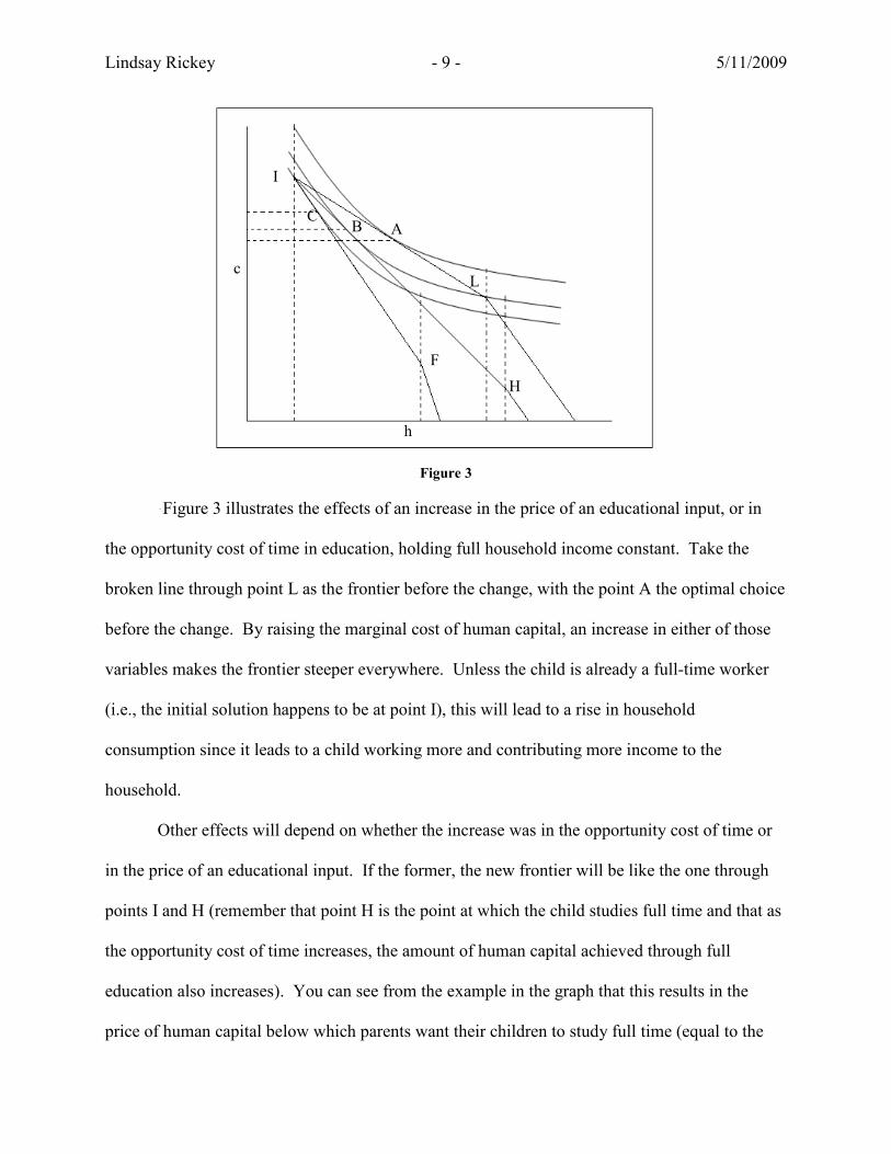
c Figure 3 illustrates the effects of an increase in the price of an educational input, or in
the opportunity cost of time in education, holding full household income constant. Take the
broken line through point L as the frontier before the change, with the point A the optimal choice
before the change. By raising the marginal cost of human capital, an increase in either of those
variables makes the frontier steeper everywhere. Unless the child is already a full-time worker
(i.e., the initial solution happens to be at point I), this will lead to a rise in household
consumption since it leads to a child working more and contributing more income to the
household.
Other effects will depend on whether the increase was in the opportunity cost of time or
in the price of an educational input. If the former, the new frontier will be like the one through
points I and H (remember that point H is the point at which the child studies full time and that as
the opportunity cost of time increases, the amount of human capital achieved through full
education also increases). You can see from the example in the graph that this results in the
price of human capital below which parents want their children to study full time (equal to the
c
h
I
L
H
F
A B C
Figure 3

Lindsay Rickey - 10 - 5/11/2009
slope of the indifference curve at the point of full education) decreasing, and the price above
which they want children to work full time (equal to the slope of the indifference curve at point
I) staying the same. Therefore, the effect of a rise in the child wage rate (or, if the child works
for his parents, in the domestic productivity of child labor) is to raise the probability of full-time
work (as the increased marginal cost is more likely to be above the maximum price the head will
pay for education), and to lower the probability of full-time study (as the increased marginal cost
is more likely to be above the maximum price at which the head will enroll their child in school
full time); the effect on the probability of part-time work is ambiguous. The effect on the
demand for educational inputs (other than the child’s own time) is also ambiguous because, on
the one hand, the demand for human capital falls, but on the other, each unit of human capital is
produced with more educational inputs and less time.
If the price of educational inputs rises, the new frontier will be the one through points I
and F. The price of human capital below which children study full time may rise or fall (in the
example in the graph, it rises); that above which they work full time is again unaffected.
Therefore, if the price of, for example, books or travel to school goes up, the probability of full-
time work increases (as marginal cost of human capital increases), but we cannot say whether the
child is more likely to study full or part time. The reason for this is that the income and
substitution effects are opposed to each other—the income effect would cause children to work
more since the household is poorer due to the price increase, but the substitution effect would
lead children to spend more time in school rather than spend money on educational inputs. If the
income effect is stronger, a child will be more likely to part-time study, and if the substitution
effect is stronger, a child will be more likely to study only.

Lindsay Rickey - 11 - 5/11/2009
We can see that the shape of the indifference curve greatly influences the head’s decision
to send a child to work, school, or both. The indifference curve, in turn, is determined by the
head’s preferences for human capital for the child and household consumption. Someone who
values education and the accumulation of human capital a great deal will have a steeper
indifference curve than one who does not value human capital. Comparing Figure 2 and Figure
4, we see that the household head with a steeper indifference curve will have a higher maximum
price of human capital and a higher minimum below which he allows the child to study full time,
which makes sense since he is willing to give up more units of household consumption for
human capital. For the particular household head in Figure 4, human capital accumulation is
important enough to devote all of the child’s time to it.
Figure 5 shows three cases where the child will never study and work at the same time,
i.e. the indifferent curves are straight lines. In these cases the maximum price at which the head
will pay for any schooling and the minimum price below which the child goes to school only are
the same, since the slope of the indifference curve is the same everywhere. The curve that
crosses point E represents an extreme valuation of human capital above consumption, while the
curve that crosses point I represents an extreme valuation of consumption above human capital.
Figure 4 Figure 5
c
h
c
h
I I
L L
E
Lindsay Rickey - 12 - 5/11/2009
The curve crossing Point L represents a high, though not extreme, valuation of human capital,
leading to the child being fully employed in education.
Many factors not explicitly modeled here could affect the value placed on human capital
versus consumption. The education level of the household head, the gender and age of the
household head, the total number of adults in the household, the total number and ages of other
children in the household, and the perceived quality of the schools could all affect how the head
views education as compared with household consumption. The head’s preferences for a child’s
education might also be dependent on the characteristics of that particular child, for example,
whether the child is their biological child.

Lindsay Rickey - 13 - 5/11/2009
3. Review of Empirical Findings
This section reviews the findings of many of the empirical studies that use micro-level data to
analyze the possible determinants of child labor and child schooling. I have divided the review
into separate subsections for the main potential factors I have found in my research on child
labor.
3.1 Poverty
3.1.1 Poverty’s Effect on Child Labor
Many theoretical models of child labor are based on what Basu and Van (1998) called the
Luxury Axiom, i.e. that a family will send a child to work only if the family’s non-child-labor
income drops below some threshold. However, despite the seemingly obvious link between
poverty and child labor, the evidence for a significant income effect is mixed. An insignificant
income effect is reported in Coulombe (1998) in Côte d’Ivoire, Sasaki and Temesgen (1999) in
Peru, Patrinos and Psacharopoulos (1997) in Peru, Ilahi (2001) for rural boys in Peru, Ray (2000)
in Pakistan, and Ersado (2005) for urban children in Nepal, Peru, and Zimbabwe. In her survey
of field studies of child labor in India, Bhatty (1998) concludes that there is no clear association
between poverty and child labor. In a review of empirical studies of Côte d’Ivoire, Ghana and
Zambia, Canagarajah and Nielsen (2001) also conclude that there is not much evidence in favor
of the view that poverty is a significant cause of child labor.
A positive coefficient on income is obtained in Cartwright (1999) for household
farm/enterprise work in rural Colombia and in Patrinos and Psacharopoulos (1995) in Paraguay.
Bhalotra and Heady (2003) provide a theoretical justification for the positive coefficient. They
explain that owning land has both wealth and substitution effects on a household’s supply of
child labor. The wealth effect suggests that large landholdings generate higher income, making it

Lindsay Rickey - 14 - 5/11/2009
easier for households to forgo the income that child labor brings. However, because of
geographical inaccessibility to workers, or lack of information flows, large landholders may find
it cheaper to hire family members rather than other labor. Bhalotra and Heady test this model by
looking at households in Ghana that run their own farms and find that richer households in
developing countries tend to own more land, and households tend to employ family members
(including children) on this land. Consequently, richer households, on average, make greater use
of child labor than poorer households. This theory is also supported by Dumas (2007), who
looks at rural households in Burkina Faso and finds that child labor seems to be due to the
absence of labor market rather than to household subsistence needs.
Negative income effects are found in Cartwright for wage work in rural Colombia (1999),
in Cigno and Rosati in rural India (2000), and in Ilahi for rural girls in Peru (1999). Amin,
Quayes, and Rives (2004) also find a negative income effect for both urban and rural boys and
girls in Bangladesh, as do Rosati and Tzannatos (2000) in Vietnam, Liu (1998) for wage work in
Vietnam, Ray (2000) in Peru, Bhalotra and Heady (2000) for rural farm work for boys in
Pakistan and girls in Ghana, and Ersado (2005) for rural children in Nepal, Peru, and Zimbabwe.
Edmonds (2005) finds that income growth in Vietnam can account for a large part of the
reduction in child labor observed there during the 1990s. Carvalho (2000) examines the
introduction of an old-age pension in Brazil and finds that it resulted in a reduction in child labor
amongst children living with grandparents, with the impact of a grandmother’s pension on her
granddaughters’ labor being especially large. Edmonds (2006) looks at how cash transfers affect
child labor in South Africa and documents large declines in total hours worked when black South
African families become eligible for social pension income. Schady and Araujo (2006) study
cash transfers in Ecuador and find that the transfers have a large negative impact on work, about

Lindsay Rickey - 15 - 5/11/2009
17 percentage points. Considering these studies have less methodological problems than cross-
sectional data (Edmonds (2001) is based on two years of data and the rest are natural
experiments), Bhalotra and Tzannatos (2003) postulate that the variance of the income effect in
different studies might come from methodological issues rather than actual country variations.
However, Bourguignon, Ferreira, and Leite (2002) and Cardoso and Souza (2004) find that, in
Brazil, conditional income transfers requiring a child to go to school had no significant impact on
the incidence of child labor.
3.1.2 Poverty’s Effect on Child Schooling
Although child labor and schooling are not mutually exclusive, and are, in fact, often
done together, it is interesting to consider whether the effect of poverty on schooling is any
stronger than the effect (or lack thereof) of poverty on child labor. Behrman and Knowles
(1999) survey estimates of income elasticities for a range of indicators of educational enrollment
and attainment for the US and a number of developing countries. The median elasticity of 0.07 is
small, though somewhat larger estimates of about 0.20 are observed for lower income regions.
In their own analysis of five indicators of schooling in Vietnam in 1996, Behrman and Knowles
find higher income elasticities than the previous literature. According to Bhalotra and Tzannatos
(2003), this is at least partly on account of Behrman and Knowles’ more careful attention to the
choice of indicators and the specification of the equation.
A significantly positive effect of income on child schooling is found in Ray (2000) for
Pakistan, Cigno, Rosati, and Tzannatos (2001) in rural India, Ilahi (2001) for girls in Peru,
Canagarajah and Coulombe (1999) in Ghana, Coulombe (1998) in Côte d’Ivoire, and Jensen and
Nielsen (1997) in Zambia. In Côte d’Ivoire, Grootaert (1999) shows that for poor households, in

Lindsay Rickey - 16 - 5/11/2009
both urban and rural areas, there is a higher probability for selecting non-schooling options than
richer households. Rosati and Tzannatos (2006) find that the effect of income on schooling in
Vietnam is non-linear and that the significantly positive effect of income on the probability that a
child will only go to school decreases with the level of income. Edmonds (2006) finds that cash
transfers in the form of pensions lead to large increases in child schooling in South Africa.
Schady and Araujo (2006) study cash transfers in Ecuador and find that the transfers have a
large, positive impact on school enrollment, about 10 percentage points, perhaps partly because
some households believed that there was a school enrollment requirement attached to the
transfers (though not monitored or enforced). Similarly, Bourguignon, Ferreira, and Leite (2002)
and Cardoso and Souza (2004) found in Brazil that conditional income transfers requiring a child
to go to school increased the likelihood of schooling.
Ray (2000) finds no significant income effect on child schooling in Peru, nor does Ilahi
(2001) for boys in Peru or Ersado (2005) for urban children in Nepal, Peru, and Zimbabwe.
Patrinos and Psacharopoulos (1995) did not find monthly family income to be a significant
determinant of years of school attainment in Paraguay, but did find a positive association with
school enrollment. A negative effect of income on child schooling is found by Patrinos and
Psacharopoulos (1997) in Peru. Overall, though, it seems that income has a bigger effect on
schooling than on child labor. In fact, higher income can lead to more schooling even in regions
where higher income leads to more child labor. For example, Bhalotra and Heady (2003) find
that in Ghana and Pakistan income has a significantly positive effect on schooling attendance
even though larger farm size leads to richer households employing more child labor.
Lindsay Rickey - 17 - 5/11/2009
3.2 Parental Education
There is consistent evidence that the mother’s education has a negative effect on child
labor, and the size of this effect is often greater than that of the father’s education. Using data
combined for boys and girls in rural and urban areas in Ghana, Canagarajah and Coulombe
(1999) find that the father’s secondary level education has a negative effect on child work
participation while the mother’s education has no effect. Using the same data, Bhalotra and
Heady (2000) find a negative effect for the mother’s middle or secondary level education for
rural boys but no effect for the father’s education. Bhalotra and Heady also find that on family
farms in rural Pakistan, the mother’s middle or secondary level education has a negative effect
for boys and girls (larger in the case of girls) and the father’s secondary education has a negative
effect that is restricted to girls.
Cigno and Rosati (2000) find that in rural India the children of mothers with less than
primary education are significantly more likely to be in full-time work as compared with full-
time study, and having a mother who completed middle school reduces the probability of
combining work and school as compared with full-time study, while the father’s education has
no significant effect. Ravallion and Wodon (1999) find negative effects of the mother’s and
father’s education level on child labor in Bangladesh. In Vietnam, years of father’s education
have no effect on child labor but mother’s education has a negative impact on the probability of
work (full-time and part-time) as well as on the probability of being neither in work nor in school
(Rosati and Tzannatos 2000). However, Liu (1998) finds insignificant effects for both mother’s
and father’s years of schooling on child labor in Vietnam, whether market or home based.
Emerson and Souza (2008) find that in Brazil, both father’s and mother’s education have a
negative effect on child labor and a positive effect on schooling for both boys and girls. Kruger

Lindsay Rickey - 18 - 5/11/2009
(2007) finds these same effects in Brazil for parents’ education.
Amin, Quayes, and Rives (2004) examine child labor in Bangladesh, dividing the
children by gender, region, and age groups: younger (aged 5-11) and older (aged 12-14). They
find that the education of the male head significantly lowers the probability of working for all
rural boys (older and younger), all urban girls, urban older boys, and rural older girls, with no
effect on urban younger boys and rural younger girls. The education of the female head has a
significantly negative effect on child labor for boys in all four groups, and for all rural girls, but
no effect for urban girls (older and younger). Bhalotra and Heady (2003) find that the father’s
education has a negative effect on the probability that rural girls in Pakistan work, but no effect
on work for rural boys in Pakistan or for rural boys and girls in Ghana. The father’s education
does, however, have a positive effect on school attendance for rural boys and girls in both
Pakistan and Ghana. The mother’s education has a significantly negative impact on child labor
for rural boys in Ghana, and rural boys and girls in Pakistan, and a significantly positive effect
on schooling for rural girls in Pakistan, and rural boys and girls in Ghana. It has no effect on
labor for rural girls in Ghana and no effect on schooling for rural boys in Pakistan.
Patrinos and Psacharopoulos (1997) find that the probability of combining work and
school as compared with the probability of full-time study is reduced by the years of the father’s
education in Peru and by years of mother’s education in Paraguay (Patrinos and Psacharopoulos
1995). Using the same Peruvian data, Sasaki and Temesgen (1999) find that the probability of
combining work and school as compared with full-time study is reduced by the father’s college
education and the mother’s secondary and college level education. While the first study uses a
binomial logit, the second uses a multinomial logit, allowing for two further outcomes: work
only and neither work nor school. The mother’s education has no effect on these outcomes

Lindsay Rickey - 19 - 5/11/2009
relative to study only, while the father’s secondary education has a negative effect on the
probability of work only relative to study only. Controlling for household-specific effects using
a random effects probit on the Peruvian data for two years (1994 and 1997), Ilahi (1999) finds a
negative effect of the education of the oldest prime-age female on the probability of children
working in an income-generating activity in Peru, and this effect is similar for rural and urban
areas. While the results of the three studies for Peru do not contradict one another, they do show
the importance of which sub-sample is being discussed and whether the education effects are
allowed to be nonlinear (Bhalotra and Tzannatos 2003).
In Colombia, multinomial logit estimates reported in Cartwright (1999) indicate that
there is a negative effect of the father’s years of schooling on the probability of full-time child
work whether this is for wages, on the family farm or enterprise, or for full-time home care (with
full-time study as the reference category). The mother’s years of schooling have no effect on
child labor producing marketable goods but have a positive effect on the probability that a child
is at home in full-time care. This result is consistent with the view that educated women are
more likely to work and so their children may have to substitute for them at home at the expense
of going to school (Bhalotra and Tzannatos 2003). These effects are similar in rural and urban
areas, though the effects of the mother’s education are stronger in urban areas. In their analysis
of child labor in urban Bolivia, Cartwright and Patrinos (1997) find a negative effect of the
mother’s years of education on the probability of children working in wage-based labor as
opposed to being in school. Unlike in the case of Colombia, there is no effect of mother’s
education on child time in home-care. They do not include the father’s education in the model.
Using a multinomial logit, Ersado (2005) finds that the years of the mother’s education
have a significantly positive effect on schooling for rural and urban children in Nepal and

Lindsay Rickey - 20 - 5/11/2009
Zimbabwe and urban children in Peru, and a significantly negative effect on child labor for rural
children in Nepal and rural and urban children in Zimbabwe. However, he finds no significant
effect of the mother’s education on schooling for rural children in Peru or on child labor for
urban children in Peru, and a significantly positive effect on child labor for rural children in Peru.
With regard to the father’s education, Ersado found no effect on schooling for urban children in
Zimbabwe and no effect on child labor for all children in Zimbabwe and rural children in Peru
and Nepal, a significantly positive effect on schooling for rural children in Zimbabwe and all
children in Peru and Nepal, and a significantly negative effect on child labor for urban children
in Peru and Nepal.
Rosati and Tzannatos (2006) also use a multinomial logit model to examine child labor in
two different years in Vietnam (1993 and 1998). They find that years of the father’s education
have a significantly negative effect on the probability a child only works as opposed to only
studies for both years and on the probability a child works and studies in the 1998 survey (again,
with “only studies” as the reference group). The father’s education has no effect on the
probability a child works and studies in the 1993 survey. The mother’s education has a negative
impact on the children only working for both years but no effect on the children working and
studying (again, for both years).
Grootaert (1999) finds that in Côte d’Ivoire, the probability of full-time study as opposed
to full-time work is positively influenced by years of the father’s education in urban areas and by
years of the mother’s education in rural areas; in each case, the education of the other parent has
no effect. For rural and urban regions, both the father’s and mother’s education raise the
probability of a child combining school with work as opposed to working full time. Analysis of
the same Côte d’Ivoire data by Coulombe (1998) using a bivariate probit shows no effect of the

Lindsay Rickey - 21 - 5/11/2009
father’s schooling on either work or school participation. The mother’s education has no effect
on work although it does increase school participation. Nielsen (1998) also finds no effect of the
father’s schooling on child work or school decisions in bivariate probit estimates of data for
Zambia, but she does not investigate mother’s schooling. Using a fixed-effect logit model,
Tunali finds no parental education effects in Turkey, but the probit analysis by Dayioglu (2006)
shows that the mother’s and father’s education levels have a strong negative correlation with
child labor in Turkey.
3.3 Land Size
The vast majority of working children live in rural areas and work on farms,
predominantly family-run farms (Bhalotra and Tzannatos 2003). As mentioned in the previous
section on poverty’s effect on labor and schooling (3.1), the lack of a labor market can lead to
children being used for labor on a large farm, despite the increased wealth that owning land
brings the household (Bhalotra and Heady 2003). In order to separate the income effect (which
should lead to decreases in child labor as land size increases) and the substitution effect (which
would lead to increases in child labor as land size increases), some measure of income must also
be included in the model. After controlling for income, the theoretical model would assume that
land size or the mere ownership of land would be positively correlated with child labor, since the
amount of land raises the opportunity cost of children’s time.
Canagarajah and Coulombe (1999) find no effect of farm size on child work participation
rates in Ghana. Distinguishing boys and girls and restricting the sample to rural farming
households, Bhalotra and Heady (2003) find a positive effect of farm size on girls’ work in rural
Pakistan and Ghana, though no effect for boys. They also find a negative effect on school

Lindsay Rickey - 22 - 5/11/2009
participation for rural girls in Pakistan, though no effect for girls in Ghana or for boys. Cigno
and Rosati (2000) find a positive effect of land size on child labor in rural India, combining data
on girls and boys. Rosati and Tzannatos (2006) find that in Vietnam, the size of cultivable land
owned by the household raises the probability that children will combine work with school and
the probability of full-time work as opposed to studying full time. They also find that relative to
study, unsurprisingly, owning land reduces the probability that a child is idle.
3.4 Household Size
Since size and composition are clearly correlated, the relation between household size
and child work will depend upon whether household composition is held constant. In empirical
results, there is a tendency to find a positive association of household size and child work.
However, this finding cannot be regarded as robust since the studies differ in whether or not land
size and household composition are held constant (Bhalotra and Tzannatos 2003). Bhalotra and
Heady (2003), controlling for these factors, find negative effects of household size on child’s
labor participation for boys in rural Pakistan and girls in rural Ghana with no effect for girls in
rural Pakistan or boys in rural Ghana. They also find positive effects of household size on child
school participation for boys and girls in rural Pakistan and girls in rural Ghana, with no effect
for boys in rural Ghana.
Cigno, Rosati and Tzannatos (2001) also find a negative effect of household size for
participation in work in rural India. Ilahi (1999) finds a negative effect on child labor for boys
and no effect for girls in Peru. Also using data from Peru, Patrinos and Psacharopoulos (1997)
find a negative effect of the number of siblings (not household size) on the probability of
combining work and school relative to the probability of simply attending school if the number

Lindsay Rickey - 23 - 5/11/2009
of children not in school is held constant (insignificant if this control variable is not included). In
Vietnam, Rosati and Tzannatos (2006), after controlling for total number of children, find a
significant negative effect of household size on the probability of being in work and on the
probability of combining work and school, relative to the probability of simply being in school
for both 1993 and 1998 surveys. There is no effect for the children who report being in neither
work nor school.
Positive estimated effect of household size on child work are found in Patrinos and
Psacharopoulos (1995), who, for Paraguay (in contrast to Peru), find a positive effect of the
number of siblings (not household size) on the probability of combining work and school relative
to the probability of simply attending school. Also, Amin, Quayes, and Rives (2004) find a
significantly positive effect of household size on all groups of boys (rural/urban, younger/older)
and all girls except urban older girls, for whom they find no effect, though they do not control for
household composition.
3.5 Household Composition
Household composition effects refer to the age and gender structure of the household.
Additional compositional effects that may be taken into account are whether both parents are
alive and whether they are present in the household (or have, for example, migrated away for
work). We would expect that the absence of a parent would create economic hardship and
increase child labor, especially if the absent parent was the primary wage earner (usually the
male).
Given that pre-school children are too young to work, and that an increase in their
number is thus equivalent to a lump-sum reduction in full income (an income-dilution effect), we

Lindsay Rickey - 24 - 5/11/2009
would expect from the theoretical model that full income raises the probability of full-time work,
lowers that of full-time study, and has ambiguous effect on that of part-time work. According to
the theoretical model, an increase in the number of school-age children, holding full income
constant, raises the probability of part-time work, and lowers that of full-time study, but has no
effect on full-time work.
Grootaert (1999) finds no clear evidence of sibling effects in Côte d’Ivoire although
Coulombe (1998), using the same data, finds that the number of children under 6 raises work
participation for older children. In Vietnam, both the number of siblings under 6 and the number
of school-age siblings (6-15 years) raise the probability of school-age children working only and
the probability of children working and studying for both 1993 and 1998 (relative to full-time
study), except siblings under 5 had no effect on working and studying in 1998 (Rosati and
Tzannatos 2006). Ilahi (1999) finds no household composition effects on child labor in Peru.
Using the same data, Sasaki and Temesgen (1999) confirm that the number of children in the
household does not affect full-time work participation of children in Peru but they find it does
increase the probabilities of doing school and work and being idle, relative to full-time study.
On the other hand, estimates of binary probit models in Ray (2000) suggest a positive effect of
the number of siblings on work probabilities in Peru. In Brazil, Emerson and Souza (2008) find
a positive effect of the number of children on the probability of child labor, and a negative effect
on the probability of school participation.
The presence of younger siblings discourages work participation amongst girls in rural
Ghana, household composition having no effect on the work hours of Ghanaian boys (Bhalotra
and Heady 2000). The same study finds that the presence of younger boys (under 10) in the
household reduces the work participation of both boys and girls aged 10-14 in rural Pakistan,

Lindsay Rickey - 25 - 5/11/2009
whereas the presence of little girls in the household has no effect. Ray (2000) uses the same
Pakistan data as Bhalotra and Heady and, aggregating over the sibling terms, finds no effects of
number of siblings on child labor. Kruger (2007) finds that in Brazil, the number of 0-5 year old
children has a positive effect on child labor and a negative effect on child schooling, and that the
number of 6-14 year old children has a positive effect on child labor, but also a positive effect on
schooling for girls (no effect on schooling for boys). Cigno, Rosati and Tzannatos (2000) find
that having both younger siblings (0-6) and siblings in one’s own age group (6-12) raises the
probability of working of school-age children in rural India. Similarly, the number of 0-6 year
old siblings raises the probability of work relative to school-only in Peru (Patrinos and
Psacharopoulos 1997). Ersado (2005) finds no effect on the number of children under 5 on the
probability that a child works in Peru or in rural Nepal, and a positive effect on this probability in
Zimbabwe and urban Nepal. He finds no effect of children under 5 on the probability of
schooling in rural Peru and Nepal, and urban Zimbabwe, and a significantly negative effect in
urban Peru and Nepal, and rural Zimbabwe.
Using data from Colombia and Bolivia respectively, Cartwright (1999) and Cartwright
and Patrinos (1999) find that having older brothers and sisters reduces the probability that a
younger child works. Canagarajah and Coulombe (1999) who use the same Ghana data find that
the number of adult males in the household has a significantly positive effect on the work
participation of 11-14 year old children in rural and urban areas, though there is no effect for 7-
10 year-olds. They find that the numbers of siblings and other compositional variables have no
effect. The presence of men and (especially) women over 60 reduces the probability that a girl in
Pakistan works, there being no effects on Pakistani boys or on Ghanaian children. Overall, the
effects of household composition are gender-specific and they are stronger in Pakistan than in

Lindsay Rickey - 26 - 5/11/2009
Ghana (Bhalotra and Heady 2000). Bhalotra and Heady also find that the number of women
over 60, though decreasing child labor, also decreases child participation in school for boys and
girls in rural Ghana, and has no effect on boys and girls in rural Pakistan (2003). In Brazil,
Kruger (2007) finds that the number of people in the household over 65 has a significantly
negative effect on child labor participation for both girls and boys, though no effect on child
schooling rates.
3.6 Gender of Household Head
The prevalence of female-headed households varies considerably across countries. It
tends to be greater in sub-Saharan Africa than in Asia. For example, it is 30% in rural Ghana as
compared with 3% in rural Pakistan (Bhalotra and Heady 2000). Most of the studies that include
female headship in their econometric model also include a measure of household income. If
female headship significantly raises child labor participation at a given level of income, then it
must indicate a degree of vulnerability of the household that is not picked up by household
income. Bhalotra and Tzannatos (2003) postulate that this could be the result of a female-headed
household’s borrowing ability or, more generally, its ability to deal with a crisis, its perception of
the range of job alternatives available to it, or its assessment of its human capital. The result is
also consistent with women being less altruistic towards children than men, but empirical
evidence indicates this is not the case (e.g. Rubalcava, Teruel, and Thomas (2009) find that
women allocate more resources toward investment in the future, Cardosa and Souza (2004) find
that cash transfers to women have a larger positive effect on schooling than transfers to men).
Support for the hypothesis that children of female-headed households are more likely to
work and less likely to be in school is found for Paraguay in Patrinos and Psacharopoulos (1995)

Lindsay Rickey - 27 - 5/11/2009
and for rural (but not urban) Côte d’Ivoire in Grootaert (1999). Bhalotra and Heady (2003) find
a positive effect of female headship on the labor participation rates of boys and girls in rural
Pakistan and for girls in rural Ghana (with no effect for boys in rural Ghana). They find no
effect of female headship on child schooling for any of the groups. Amin, Quayes, and Rives
(2004) find that in Bangladesh, female headship is positively correlated with child labor for most
of the groups of children (except for rural older boys, where there is no effect). Ersado (2005)
finds no effect of female headship on schooling or labor for the majority of the children in Nepal,
Peru, and Zimbabwe. He does find a negative effect of female headship on child labor in urban
Zimbabwe, but also a negative effect on schooling in rural Nepal and urban Zimbabwe.
Canagarajah and Coulombe (1999) do not separate the data by gender and they find that the
indicator for female headship is insignificant. Although he does allow gender-specific effects,
Ilahi (1999) finds no role for female headship in Peru.
Ray (2000) finds no relationship between child labor and female headship for children in
Peru and Pakistan, but does find a positive relationship between female headship and schooling
for girls in Pakistan (no effect for the boys in Pakistan or children in Peru). This is consistent
with empirical evidence indicating that the higher altruism of mothers is often focused more on
girls than boys (e.g. Duflo (2003) finds that grandmothers give more of their pension to their
grandchildren than grandfathers, and more to granddaughters than grandsons).
3.7 Marital Status of Household Head
As with female headship, the effect of the marital status of the household head on child
labor and schooling cannot come from differences in income levels, since income is controlled
for in most of the empirical studies. The other possible reasons might be similar to those for
Lindsay Rickey - 28 - 5/11/2009
female headship (such as borrowing ability), and we might also expect that female headship and
the head being single are correlated. Since most studies do not control for the head being single,
female headship might have a positive effect on child labor because many female heads are also
single, and hence have an additional burden in their ability to borrow money. Also, if the effect
of parents’ characteristics differ according to the parent’s gender, e.g. if the mother’s education
has a larger effect on child labor and schooling than the father’s education, the effect of the
parent being single would depend on the gender of the remaining parent. We would also expect
that these gender differences would remain even if the household head is not the biological
parent of the child (e.g. an uncle or grandparent).
Cardosa and Souza (2003), one of the few studies that controls for the marital status of
the household head, find that in Brazil the absence of the father has a significantly negative
impact on schooling and on child labor for boys but no effects for girls. The absence of the
mother has a significantly negatively correlation with schooling for boys (though less of an effect
than the father’s absence), a significantly negatively correlation with schooling for girls, and a
significantly positively correlation with labor for boys with no effect on labor for girls. These
results indicate that effects do change depending on the gender of the remaining parent, and that
these effects also change based on the gender of the children. According to these results, boys
are generally more affected by the parent being single than girls, though the magnitude and even
the direction of the effect will depend on the gender of the remaining parent.
3.8 Age of Household Head
This is an indicator of the stage of the lifecycle that the household is at. If the oldest male
reports as head, this variable may also indicate whether the child lives in a vertically extended

Lindsay Rickey - 29 - 5/11/2009
household, with grandparents. If the equation also includes a full set of age-gender variables that
reflect household composition, the age of the household head has a less clear meaning and a
weaker role to play (Bhalotra and Tzannatos 2003). Perhaps because of this fact, most studies do
not include this in their model. Those studies that do include it and find it significant do not have
full controls for household composition, e.g. Nielsen (1998), Ray (2000), Cardoso and Souza
(2003), Ersado (2005), and Emerson and Souza (2008).
3.9 Relation to Head
Households in developing countries are large and complex and often contain not just
vertical but also horizontal extensions (Bhalotra and Tzannatos 2003). As a result, nephews,
nieces, sisters-in-law, and grandchildren may be counted amongst children along with sons and
daughters of the head of household. Additionally, in sub-Saharan Africa, there is a high
prevalence of child fostering and orphans. Assuming that the head plays the primary role in
decisions regarding child labor, an interesting hypothesis is that the children of the household
head are preferred and hence less likely to work.
Cockburn (2001) investigates this variable in probit estimations for work and school in
Ethiopia and finds that children of the household head are more likely to attend school. In
contrast, Bhalotra and Heady (2003) find that children of the head are more likely to be in work
in rural Pakistan but in rural Ghana, sons are less likely to be in work (no effect for daughters).
They also find no effect on schooling for sons in rural Pakistan or for sons and daughters in
Ghana, but a negative effect on schooling for daughters in rural Pakistan. However, Blunch and
Verner (2001), also analyzing data from Ghana, find that being the child of the head is positively
correlated with child labor for rural boys, negatively correlated for urban girls, and has no effect

Lindsay Rickey - 30 - 5/11/2009
on rural girls or urban boys. Jensen and Nielsen (1997) find that in Zambia having a non-
biological relation to the head of household negatively affects the probability of attending school.
Given the increasing proportion of orphaned children in Africa (Subbarao, Plangemann, and
Mattimore 2001), it is important to investigate whether outcomes are different for children living
with adult caretakers other than their parents. Based on data from Uganda, Bishai et al. (2003)
show that biological relatedness is a strong predictor of the quality of care offered to children.
Evidence from the Demographic and Health Surveys for 10 countries in sub-Saharan
Africa in which households were interviewed between 1992 and 2000 shows that orphaned
children in Africa live, on average, in poorer households and are significantly less likely than
other children to be enrolled in school. The lower school enrolment of orphans as compared
with other children is not explained by their greater average poverty since orphans are less likely
to be in school than non-orphans with whom they co-reside. This suggests that distant relatives
and unrelated caregivers invest less in orphaned children than in their own children or closer
child relatives (Case, Paxson and Ableidinger 2004).
3.10 Child Gender
The effect of a child’s gender on their labor and schooling varies widely by country, and
has a great deal to do with the cultural norms of that country. These can affect parents’ attitudes
towards their children, the returns to education, the opportunity cost of education—all of which
in turn affect child labor and schooling decisions. There is also a great deal of evidence that the
effects of other variables on child labor and schooling change according to gender, indicating
that the determinants for male and female child labor and schooling should be considered
separately.

Lindsay Rickey - 31 - 5/11/2009
Liu (1998) finds that the probability of engaging jointly in schooling and market work is
significantly higher for boys than for girls in Vietnam, while the probability of engaging jointly
in school and house work is higher for girls than for boys. Cartwright and Patrinos (1999) in
Bolivia find that boys are more likely to work full time than are girls. In Colombia, Cartwright
(1999) finds that boys are more likely to work than girls, but girls are more likely to be working
full time (as compared to combining work and school). Rosati and Tzannatos (2006) use a
multinomial logit model to show that females are more likely to be working full time (compared
to full-time study), and that they are just as likely to be combining work and school (relative to
full-time study). Ersado (2005) finds that girls are more likely to work in Nepal and Zimbabwe.
For children in Pakistan (Ray 1998), Peru (Ray 1998, Ersado 2005), Paraguay (Patrinos
and Psacharopoulos 1995), Ecuador (Sasaki 2000), and for older children (aged 12-14) in
Bangladesh (Amin, Quayes, and Rives 2004), it is found that girls are less likely to work than
boys. Results from Côte d’Ivoire (Grootaert 1999, Coulombe 1998) are slightly different—while
girls are less likely to engage in work and schooling activities than only work, they are more
likely to undertake household work. Deb and Rosati (2004) find that girls are more likely to be
idle (neither work nor school) in Ghana and India, but assert that this may just reflect the fact
that girls are expected to perform household chores (which are not picked up by their surveys).
Some studies find no significant differences in gender patterns of work. In Ghana,
Canagarajah and Coulombe (1999), find that there is no significant difference in the probability
of being economically active between male and female children. However, using more recent
data, Blunch and Verner’s (2000) estimation shows that Ghanaian girls are slightly more likely
to work than boys. In Zambia, Nielsen (1998) finds no significant difference in participation
rates between boys and girls. Amin, Quayes, and Rives (2004) find no difference in child labor

Lindsay Rickey - 32 - 5/11/2009
for younger girls and boys (aged 5-11) in Bangladesh.
Ray (1998) finds that males attend school more than females in Pakistan. In Ghana,
Canagarajah and Coulombe (1999) find that boys are more likely than girls to attend school.
Similarly, school enrollment is higher for boys than for girls in Zambia (Nielsen 1998), Côte
d’Ivoire (Grootaert 1999, Coulombe 1998), Nepal and Zimbabwe (Ersado 2005).
However, in some countries in Latin America (Colombia, Paraguay, Nicaragua), studies
find that girls are much more likely to go to school than boys. Boys often leave school after
completing the basic primary cycle while girls continue schooling for a few more years. This
finding is consistent with the higher labor force participation of boys mentioned earlier.
However, Ersado (2005) finds that in Peru, despite females being significantly less likely to
work, they are significantly less likely to go to school. In Vietnam, Liu (1998) finds that there is
no gender difference in the predicted probability of falling in the category of “school only” –
there is no discrimination against girls with respect to educational opportunities.
3.11 Child Age
The theoretical model would expect older children to be more likely to engage in labor
activities (especially wage work) as the returns to participating in the labor market are likely to
be higher, raising the opportunity cost of the child’s time. Also, as the child ages, they are less
likely to be required to attend school by compulsory schooling laws, which usually set the
minimum age to quit school at around 14 or 15 in developing countries. With compulsory
schooling laws and diminishing returns to education, children are less likely to go to school as
they get older as well. However, a quadratic effect should also be allowed, since very young
children are probably less likely to go to school as well.
Lindsay Rickey - 33 - 5/11/2009
In Bangladesh, Amin, Quayes, and Rives (2004), using a linear term for age, find that
child labor increases with age for rural and urban older boys (aged 12-14), rural younger boys
(aged 5-11), and urban younger girls, but has no effect for urban younger boys, urban older girls,
and rural older and younger girls. In Ray’s (1998) study on Peru and Pakistan, participation rates
in labor activities increase with age in both countries. In both countries, data show that child
labor increases with age – though in Pakistan older girls are less likely to participate in the labor
force – perhaps as a result of cultural factors that militate against girls working – especially
against them being engaged in market work. However, girls are likely to remain engaged in
household work as they grow older. For the case of Columbia, Cartwright (1999) finds that the
probability of children working increases with age. In urban Bolivia, Cartwright and Patrinos
(1999) find that age increases the probability that a child will work (full time or a combination of
work and school). Similar results with respect to age are found for Côte d’Ivoire (Grootaert
1999), Paraguay (Patrinos and Psacharopoulos 1995), the Philippines (Sakellariou and Lall
1999), Turkey (Tunali 1997), Ecuador (Sasaki 2000), Bangladesh (Ravallion and Wodon 1999),
Brazil (Emerson and Souza 2008), and Ghana and Pakistan (Bhalotra and Heady 2003).
Rosati and Tzannatos (2006) in Vietnam use a multinomial logit model and find that age
has a quadratic (concave) effect on the probability that a child works only and the probability
that a child works and studies, relative to study only. According to Ray (1998), the school
enrollment rate is 90 percent for children aged 6 years in Peru, and it peaks at 9 years of age (98
percent) and then steadily falls to 62 percent by 17 years of age. In Pakistan, the school
enrollment rate starts at 65 percent for children aged 10 year and peaks at 11 years of age (70
percent). It steadily falls to 40 percent by 17 years of age. This quadratic relationship between
attendance and age is also demonstrated by Rosati and Rossi’s (2003) analysis for Pakistan and

Lindsay Rickey - 34 - 5/11/2009
for Nicaragua. Coulombe (1998) finds that for Côte d’Ivoire, there is a quadratic relationship
between school enrollment and age, with enrollment peaking at 11 years. Liu (1998) allows a
quadratic relationship in her multinomial logit model for Vietnam. She finds that the probability
of schooling increases with age till the age of 11 and then falls slightly. Similar results are
obtained in a study of Bangladesh (Ravallion and Wodon 1999) and Ghana (Canagarajah and
Coulombe 1999, Bhalotra and Heady 2003). Other studies that have used a linear variable for
age usually find a negative relationship between schooling and age, including Patrinos and
Psacharopoulos (1997) in Peru, Ersado (2005) in Nepal, Peru, and Zimbabwe, and Bhalotra and
Heady (2003) in Pakistan.
3.12 Region Effects
Within countries, rural areas support a higher incidence of child labor than do urban areas
for nearly all of the empirical studies surveyed here (the one exception being Bangladesh, in
Amin, Quayes and Rives (2004), where urban areas have significantly higher labor rates). Since
most of the studies control for household income, a higher percentage of poverty in rural areas is
not a sufficient reason. Bhalotra and Tzannatos (2003) offer other possible reasons: relatively
weak school infrastructure and lower rates of technical change in rural areas may discourage
school attendance. Children may also be more easily absorbed into the informal economies of
rural areas, on account of the prevalence of self-employment, relatively low skill requirements in
agricultural work, and the greater degree of market imperfection in rural regions. As with child
gender, there is considerable evidence that the determinants of child labor and schooling change
depending on whether the region is rural or urban, indicating that regressions should be done
separately for these two groups.
Lindsay Rickey - 35 - 5/11/2009
3.13 Community Infrastructure Effects
Besides the importance of the presence and quality of schools on child labor and
schooling decisions, other measures of community infrastructure, such as access to public
transport, safe drinking water, and electricity, often play a role in whether a child will work
and/or go to school. We would expect communities with better, more established infrastructure
to have higher school attendance since the costs would be less (if the school is closer or if there
is public transportation) and/or the benefits greater (if the quality of the school is better).
Examining child labor and schooling in rural areas of Ghana and Pakistan, Bhalotra and
Heady (2003) find that the presence of a girls’ primary school has no effect on children in Ghana
or Pakistan, but a boys’ primary school increases the probability that girls will work in Pakistan
with no effect for boys. Surprisingly, the presence of a girls’ primary school significantly lowers
the probability that a girl in Pakistan will attend school but raises the probability that a boy in
Ghana will attend school (no effect for boys in Pakistan or girls in Ghana). The presence of a
middle school and/or a secondary school significantly lowers the probability of working for boys
and girls in Ghana (with no data available for Pakistan), but has no effect on child schooling
rates. The availability of public transport also lowers the probability of work in both countries,
but only for girls. Public transport also raises the probability of schooling for boys in Pakistan,
but lowers it for boys and girls in Ghana (with no effect on girls in Pakistan). Blunch and Verner
(2001), also analyzing data from Ghana, find that the distance to the nearest primary school is
significantly correlated with child labor for rural children, but not urban children; the same result
is true of distance to the nearest secondary school. This is probably the result of the scarcity of
schooling in rural areas due to their geographic isolation. This could also help explain why rural
areas have a higher incidence of child labor and lower child schooling rates than urban areas

Lindsay Rickey - 36 - 5/11/2009
Ersado (2005) finds that in rural Nepal, the number of schools in the area is positively
correlated with schooling, but has no effect on child labor (no data for number of schools
available for urban Nepal, or for Peru and Zimbabwe, the other two countries he surveys). Also,
having electricity is positively correlated with schooling for urban children in Peru and
negatively correlated with child labor for rural children in Nepal (no effect for Zimbabwe or for
other groups in Peru and Nepal); bad water storage is positively correlated with child labor in
rural Nepal and rural Zimbabwe, but also positively correlated with schooling for rural
Zimbabwe and urban Nepal. In Ray (2000), having electricity lowers the probability of child
labor for boys in Peru, but raises it for girls in Pakistan, with no effect on girls in Ghana and boys
in Pakistan. Having electricity also significantly raises the probability of girls in Peru and boys
in Pakistan going to school, with no effect on boys in Peru or girls in Pakistan. Bad water
storage is significantly positively correlated with child labor for boys in Pakistan, and negatively
correlated for girls in Peru, with no effect for girls in Pakistan and boys in Peru; it is also
significantly negatively correlated with child schooling for boys and girls in Pakistan, but has no
effect on schooling for children in Peru.

Lindsay Rickey - 37 - 5/11/2009
4. Methodology
My selection of which community, household, and child characteristics to consider is
based on previous studies on child labor, detailed in depth in the previous section, the theoretical
model, and on what data is available. The data set I am using comes from the Philippines’ 2001
Survey on Children 5-17 Years Old (SOC), a nationwide survey which provides estimates on the
number of Filipino working children between ages 5 and 17 years, their characteristics and those
of the households to which they belong. The 2001 SOC is a collaborative effort between the
Philippines’ National Statistics Office (NSO) and the International Labor Organization’s
International Program on the Elimination of Child Labor (ILO-IPEC). It has a national sample
of 26,964 sample households, 17,454 of which were found to have members whose ages were 5-
17 years old. Out of these, 17,444 households (99.9%) responded (NSO, p. 5).
The data set has data on sex, age, and education for each individual in the household and
household data on gross monthly income, expenditures, land ownership, access to drinking water
and electricity, and participation in governmental assistance programs. For children ages 5-17,
they also included data on what the child does on a day to day basis—worked, looked for work,
studied, did housekeeping and/or was idle. There is also a second survey for all children who
said that they had worked (not including housekeeping) in the last twelve months, which asked
detailed questions about what kind of work they were doing—how many hours, whether it was
risky or not, its effect on health and school, etc.
Much of the previous literature uses the probability that a child has worked in the last
twelve months as their measure of child labor, and I wanted to see if the results changed at all
based on a narrower definition of child labor. The International Labor Organization defines
child labor as work that is “mentally, physically, socially or morally dangerous and harmful to

Lindsay Rickey - 38 - 5/11/2009
children” and/or “interferes with their schooling: by depriving them of the opportunity to attend
school; by obliging them to leave school prematurely; or by requiring them to attempt to
combine school attendance with excessively long and heavy work” (ILO-IPEC, p. 16).
However, the ILO also admits that “whether or not particular forms of ‘work’ can be called
‘child labour’ depends on the child’s age, the type and hours of work performed, the conditions
under which it is performed and the objectives pursued by individual countries” (ILO-IPEC, p.
16).
With such a vague definition, I tried to be as conservative as possible in my definition of
child labor. If a child’s work was hazardous, in bad conditions, at night, caused emotional or
mental stress, or entailed heavy physical labor, I defined that as child labor, regardless of the
child’s age, under the reasoning that these conditions were “harmful to physical and mental
development” (ILO-IPEC, p. 16). The latter half of the definition, i.e. that work must not
interfere with schooling, depends a great deal on the child’s age, though the ILO specifies that
only light work can be allowed before the age of completion for compulsory schooling, which in
the Philippines is fourteen. I included in my definition of child labor any child that was fourteen
or under and not attending school, as well as those fourteen and under working nine hours or
more per day (regardless of how many days per week they worked) and/or working five hours or
more per day for more than two days per week, on the grounds that long hours would interfere
with their schooling.
Unfortunately, the survey only asked children who said they were working if they
attended school. Because of this, I could not construct a variable for whether a child was in
school unless I limited the sample to those working children. Though the question of what
causes a child to go to school when already working is an interesting one, I wanted to be able to
Lindsay Rickey - 39 - 5/11/2009
use the whole sample of children in my analysis. To do this, I used the probability that a child
studies, which is a question they ask all children ages 5 to 17. This is not a perfect proxy for
school attendance, but it still has similar social and economic consequences. In areas with poor
school quality, studying might actually be a better measure of human capital accumulation than
school attendance alone.
The independent variables I chose are based on previous literature and the theoretical
model. On the household level, I have included monthly expenditure, which in this dataset is
given in six levels rather than as a continuous variable. Following previous literature, I am using
expenditures rather than incomes, since agricultural incomes are volatile, making measured
income sensitive to the reference period of the survey. I also included the region of the
household (rural or urban), and if the household has land. Unfortunately, the survey did not
include questions about the size of the land, but evidence that houses with land have higher child
labor rates than those without also supports Bhalotra and Heady’s hypothesis that one of the
causes of child labor is the lack of a labor market (described in Section 3.1.1). Instead of only
controlling for household size, I have followed some of the previous literature and accounted for
the composition by dividing the household into different age groups and gender. The household
composition variables I am looking at are the total number of children under 5, the total number
of children aged 5 to 17, the total number of adults aged 18 to 59, and the total number of adults
who are 60 or older in the household. All of these groups are also divided by gender.
I have accounted for various characteristics of the household head, including gender, age,
marital status, and his or her education level. Though previous studies consider characteristics of
both parents, my model assumes that the household head, regardless of relation to the child,
makes the decisions regarding child activities. Over 15% of children in the survey are not the

Lindsay Rickey - 40 - 5/11/2009
biological children of the head, indicating that the parents of the children are not always the main
decision makers in households in the Philippines. I have also interacted whether the head is
single with whether the head is female to see if being single affects a female-headed household
more than a male-headed household.
The characteristics for individual children I am considering are age, gender, and whether
the child has a strong biological relationship to the household head, i.e. is the son/daughter,
brother/sister, or grandchild, as opposed to more distant relatives or completely unrelated
children. Following previous literature, I have added a quadratic term for age. Though the
theoretical model also focuses on child wage, there is no reliable data available in the dataset,
and the issue of endogeneity also makes it difficult to interpret the effect of wage. There is only
wage data for children who work, so wage, at least as it is measured here, is not an appropriate
proxy for the opportunity cost of labor. The closest proxy is whether or not the household has
agricultural land, since owning land would increase the marginal product of labor (and therefore
the opportunity cost of education) since the children can most likely work more easily and
efficiently on their own land.
For community characteristics, I am using access to drinking water and electricity, and
also a variable for whether the household is aware of a community organization in their area to
see if there are positive effects from local organizations. There is no data on the availability,
quality, or costs of schools, unfortunately, so I have to use access to drinking water and
electricity and the presence of a community organization as signals of the community’s
infrastructure, of which schools are a part. I have also added a variable for whether a family is
aware of government welfare programs to examine the possible effects of government programs
designed to help poor families. I interacted this variable with the gender of the household head
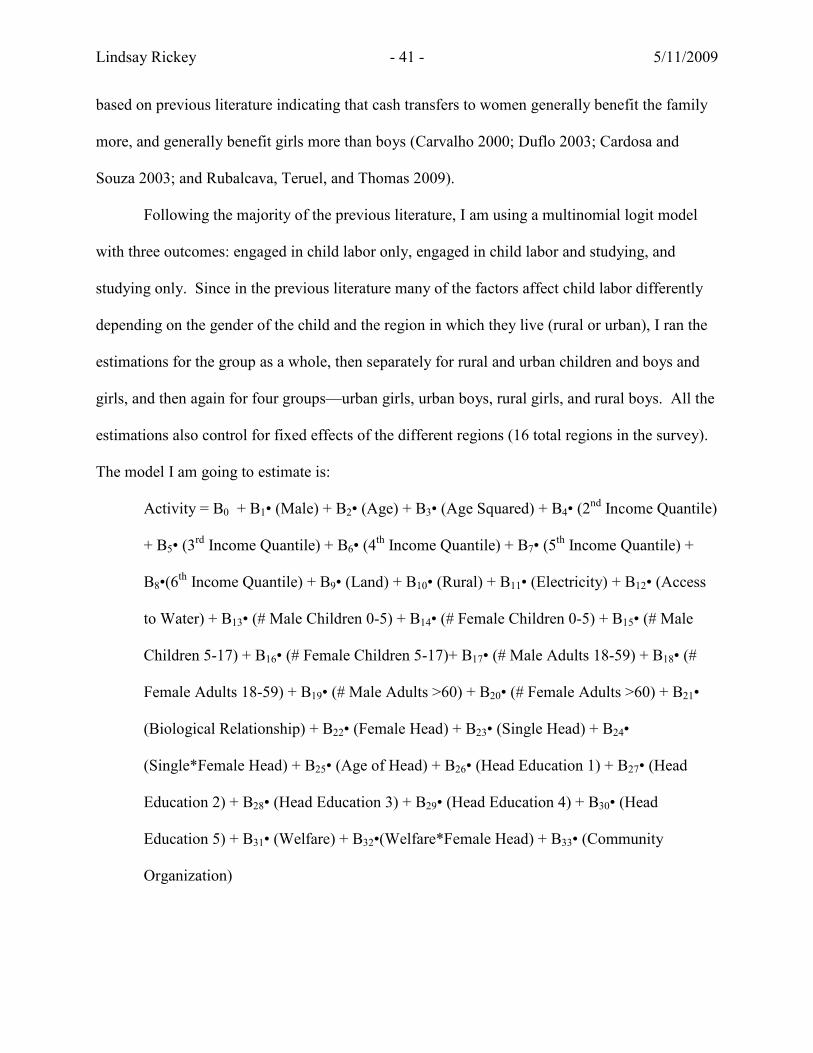
Lindsay Rickey - 41 - 5/11/2009
based on previous literature indicating that cash transfers to women generally benefit the family
more, and generally benefit girls more than boys (Carvalho 2000; Duflo 2003; Cardosa and
Souza 2003; and Rubalcava, Teruel, and Thomas 2009).
Following the majority of the previous literature, I am using a multinomial logit model
with three outcomes: engaged in child labor only, engaged in child labor and studying, and
studying only. Since in the previous literature many of the factors affect child labor differently
depending on the gender of the child and the region in which they live (rural or urban), I ran the
estimations for the group as a whole, then separately for rural and urban children and boys and
girls, and then again for four groups—urban girls, urban boys, rural girls, and rural boys. All the
estimations also control for fixed effects of the different regions (16 total regions in the survey).
The model I am going to estimate is:
Activity = B0 + B1• (Male) + B2• (Age) + B3• (Age Squared) + B4• (2nd Income Quantile)
+ B5• (3rd Income Quantile) + B6• (4
th Income Quantile) + B7• (5th Income Quantile) +
B8•(6th Income Quantile) + B9• (Land) + B10• (Rural) + B11• (Electricity) + B12• (Access
to Water) + B13• (# Male Children 0-5) + B14• (# Female Children 0-5) + B15• (# Male
Children 5-17) + B16• (# Female Children 5-17)+ B17• (# Male Adults 18-59) + B18• (#
Female Adults 18-59) + B19• (# Male Adults >60) + B20• (# Female Adults >60) + B21•
(Biological Relationship) + B22• (Female Head) + B23• (Single Head) + B24•
(Single*Female Head) + B25• (Age of Head) + B26• (Head Education 1) + B27• (Head
Education 2) + B28• (Head Education 3) + B29• (Head Education 4) + B30• (Head
Education 5) + B31• (Welfare) + B32•(Welfare*Female Head) + B33• (Community
Organization)

Lindsay Rickey - 42 - 5/11/2009
For easier reference, I have included a list with variable names and descriptions.
Name Description
Activity Categorical variable equal to 0 if a child is only engaged in child labor, 1 if engaged in both child labor and studying, and 2 if studying only
Male Dummy variable equal to 1 if the child is male, and 0 if female Age Age of the child (years)
Age Squared Age of the child squared (years squared) 2nd Income Quantile Dummy variable equal to 1 if household has average monthly
expenditure of PhP2000-2999 (baseline is households spending less than PhP2000)
3rd Income Quantile Dummy variable equal to 1 if household has average monthly expenditure of PhP3000-4999
4th Income Quantile Dummy variable equal to 1 if household has average monthly expenditure of PhP5000-9999
5th Income Quantile Dummy variable equal to 1 if household has average monthly expenditure of PhP10000-14999
6th Income Quantile Dummy variable equal to 1 if household has average monthly expenditure of over PhP15000
Land Dummy variable equal to 1 if household has agricultural land
Rural Dummy variable equal to 1 if household is in a rural region
Electricity Dummy variable equal to 1 if household has electricity
Access to Water Dummy variable equal to 1 if household’s main source of drinking water is a community water system or a tubed/piped well (as opposed to dug well, river, rain)
# Male Children 0-5 Number of male children under 5 in the household
# Female Children 0-5 Number of female children under 5 in the household # Male Children 5-17 Number of male children aged 5-17 in the household # Female Children 5-17 Number of female children aged 5-17 in the household # Male Adults 18-59 Number of male adults 18-59 in the household # Female Adults 18-59 Number of female adults 18-59 in the household # Male Adults >60 Number of male adults 60 or older in the household # Female Adults >60 Number of female adults 60 or older in the household Biological Relationship Dummy variable equal to 1 if child is the household head’s son,
daughter, brother, sister, or grandchild
Female Head Dummy variable equal to 1 if household head is female Single Head Dummy variable equal to 1 if household head is single Single*Female Head Dummy variable equal to 1 if household head is single and female Age of Head Age of the household head (years) Head Education 1 Dummy variable equal to 1 if household head’s highest level of
education is elementary graduate (baseline is no school or not enough school to graduate elementary)
Head Education 2 Dummy variable equal to 1 if head’s highest level of education is high school (not graduating)
Head Education 3 Dummy variable equal to 1 if head’s highest level of education is
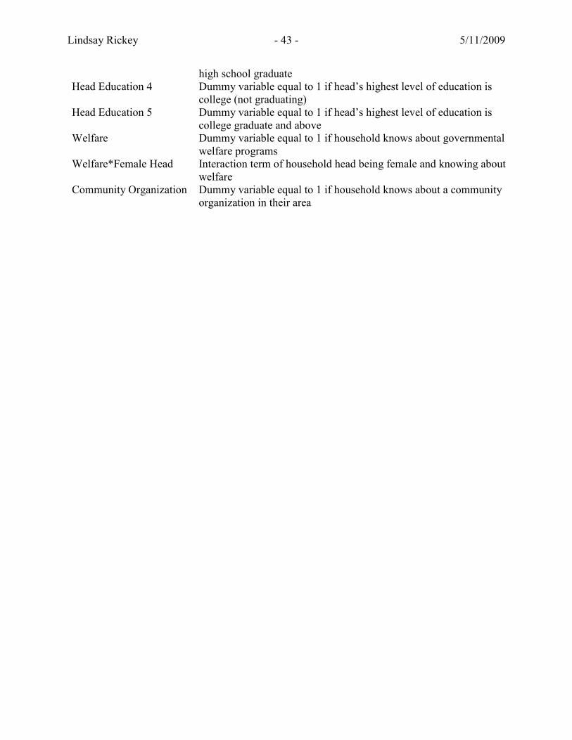
Lindsay Rickey - 43 - 5/11/2009
high school graduate Head Education 4 Dummy variable equal to 1 if head’s highest level of education is
college (not graduating) Head Education 5 Dummy variable equal to 1 if head’s highest level of education is
college graduate and above Welfare Dummy variable equal to 1 if household knows about governmental
welfare programs Welfare*Female Head Interaction term of household head being female and knowing about
welfare Community Organization Dummy variable equal to 1 if household knows about a community
organization in their area

Lindsay Rickey - 44 - 5/11/2009
5. Results
Table 1 shows the estimation results for the full sample, and separate results for rural and
urban, and boys and girls, while Table 2 shows the results for four separate groups: rural boys,
rural girls, urban boys, and urban girls. From Table 1, we can see that males are more likely to
be engaged in child labor (part time and full time) relative to studying than females, and the
effect is strong in both rural and urban areas. Children in rural areas are also more likely to work
both part time and full time than those in urban areas though the effect is stronger for boys. This
is consistent with the majority of previous empirical evidence. However, being in a rural area,
though it does affect the probability a girl will labor and study, has little effect on whether a girl
will labor full time or not.
Overall, the results show strong support for the Luxury Axiom in rural areas, i.e. as
households become richer, their children are less likely to be engaged in child labor (both part
time and full time) than to only study. Income is not as strong a determinant in urban areas,
especially for girls. In fact, for urban girls, children are actually more likely to be engaged in
part-time child labor than only studying as income increases, though the effect on labor only is
insignificant. However, since the income data is top-coded, the effects of income might actually
be understated in the results. Households in the bottom five (out of six) income quantiles,
accounting for more than 90% of the surveyed households, spend less than PhP15,000 a month,
which is approximately equal to $9184 a year (in 2001 PPP terms) (see Table 11 in the
Appendix). Considering the average household has over six people in it, the per capita
expenditure is quite low for the majority of survey respondents. Even at these low levels of
income, an increase in income still reduces child labor (part time and full time) for rural children
and for urban boys (though the effect on part-time labor is not significant).

Lindsay Rickey - 45 - 5/11/2009
The significance of income for rural children and the insignificance for urban children is
consistent with Ersado’s (2005) study of Peru, Nepal, and Zimbabwe and Canagarajah and
Coulombe’s (1999) study of Ghana. The positive effect of income on the probability that an
urban girl studies and labors relative to only studies could be due to Bhalotra and Heady’s (2003)
hypothesis that richer households with a larger amount of land use more child labor. Though
there is a control in this model for whether the household has agricultural land, there is no
measure of the size of that land, and merely owning land does not seem to be correlated with
income level (see Table 11 in the Appendix). However, it seems strange that this effect would
be present for girls but not boys and in urban areas but not rural areas. This could also result
from the endogeneity of income, since children’s income contributes to household income.
Endogeneity problems would lead to understatements of the effect of income or even positive
effects, since total household income would increase as the child worked more. Endogeneity
also explains why households in the second income quantile do not generally have significantly
less labor than those in the bottom quantile, and actually have significantly more in the case of
urban girls. These households might have been in the bottom quantile of income if their children
were not working.
The strong significance of electricity and the slightly weaker significance of access to
drinking water, in reducing labor both part-time and full-time for all groups indicate that
community infrastructure is important. Of course, these are also possible measures of wealth,
and might even be better measures of wealth, since they are not endogenously determined.
Electricity and access to water could also be correlated with other aspects of community
infrastructure, like public transport and schools. The presence of schools and transportation
would decrease the costs of schooling. The theoretical model predicts that full-time work will

Lindsay Rickey - 46 - 5/11/2009
decrease as educational expenses decrease. The effect on part-time work depends on the relative
sizes of the income and substitution effects. The income effect, i.e. that lower educational costs
mean increased income, would lead to children working less due to the increase in income. The
substitution effect would lead to children studying less since the decrease in educational costs
means that students can get more human capital for a decreased amount of studying time. In the
results, the probability of full-time work is significantly lower in the presence of electricity and
access to drinking water, as the model predicts. Since part-time work also decreases, the income
effect must dominate the substitution effect. This assumes that electricity and access to drinking
water are related to schooling costs.
Owning agricultural land is strongly correlated with working and studying rather than just
studying. If we assume that the opportunity cost of education is higher for children in
households with land (since they can more easily and efficiently work their own land), the
theoretical model would predict that full-time work would increase and full-time studying would
decrease. Though there is evidence to support the latter, full-time work does not increase
significantly. Moreover, for rural girls, land has no effect on labor at all. Since the land measure
only indicates the presence of land, rather than the size of the land, it is possible that many
households have small plots (the fact that many of the households with land are quite poor
supports this supposition, see Table 11). With such a small plot, there may be enough labor to
productively work on the land without having to take a child out of school, and so having land
does not inhibit the children from working and studying.
Unsurprisingly, age is positively correlated with engaging in child labor, often with a
quadratic effect. It is interesting to note, though, that age is insignificant in determining whether
girls (both rural and urban) are engaged in child labor full time. Household composition,
Lindsay Rickey - 47 - 5/11/2009
income, and especially the biological relationship with the household head are more important
determinants of the probability a girl will work full time. Having a strong biological relationship
with the head is negatively correlated with working full time for all groups, but the effect is
stronger for girls, and the strongest for urban girls. This is consistent with the hypothesis that the
household head is less altruistic to distant relatives and foster children, and this effect is
particularly strong for girls.
The effects of household composition are different among the different groups, though
for all groups there is evidence that a higher number of children in the household leads to more
child labor. The presence of younger children has a stronger effect in most cases, as we would
expect from the theoretical model. Pre-school children are too young to work, and so an increase
in their number, holding income constant, is equivalent to a reduction in full income (an income-
dilution effect). According to the theoretical model, a decrease in income will raise the
probability of full-time work, and lowers that of full-time study. These predictions are consistent
with the results. An increase in the number of school-age (5-17) children, though also lowering
total income per household member, should have less of an effect since they can earn income as
well. The results are consistent with these predictions in general, as the effects of the total
number of school-age children are negligible or at least smaller than the effects of pre-school
children for all of the groups. The number of school-age children can still have a significant
effect, especially if a child’s siblings, though school-age, are much younger than the child.
The effect of the number of adults is variable, and depends on the age and gender of the
adult as well as the region and gender of the child. Older female adults play the most important
role in reducing child labor and increasing studying, though young and middle-aged female
adults are important as well. The number of male adults, on the other hand, is generally less
Lindsay Rickey - 48 - 5/11/2009
significant in reducing child labor, and for urban girls and boys, is even positively correlated
with child labor. This may be reflective of different levels of altruism in males and females or
their different views on the benefits of schools versus labor. The age of the household head is
mostly insignificant, as expected, since the average age of the household is already accounted for
by the controls for household composition.
Female headship plays a mostly insignificant role, as does the head being single and the
interaction of the two. Though female headship appears highly significant for rural boys, all of
the female heads are single in households where rural boys work full time, making these results
difficult to interpret. When I excluded the interaction term from the estimation, female headship
had an insignificant effect. A single male head does lower the probability of rural boys working
part time (relative to only studying), while a single female head raises it. A single head, male or
female, raises the probability that rural girls are engaged only in child labor.
The education level of the household head is strongly negatively correlated with the
probability of being engaged only in child labor for all groups, and also with the probability of
part-time work for all groups except rural girls. This is consistent with most of the previous
literature. Since income is already controlled for, this cannot only reflect that household heads
with more education are richer. However, since expenditures are only a proxy for income, the
years of education of the household head might capture some permanent income effects.
Moreover, more educated heads might have a better knowledge of the returns to education and/or
be in a better position to enable their children to exploit the earning potential acquired through
education. In this case, the head’s education could be a proxy for returns to education.
The effect of government programs, specifically welfare and community organizations,
seems relatively weak, and only present for rural boys. In fact for urban boys, knowledge of

Lindsay Rickey - 49 - 5/11/2009
welfare programs is actually positively correlated with working. This weak effect is most likely
due to the small number of people who actually know about these programs (see Table 11 in the
Appendix). Those who do know about the programs are generally more well off. Similarly,
community organizations are generally in areas that are relatively richer, reducing the impact
they might otherwise have on child labor and schooling (Table 11).

Lindsay Rickey - 50 - 5/11/2009
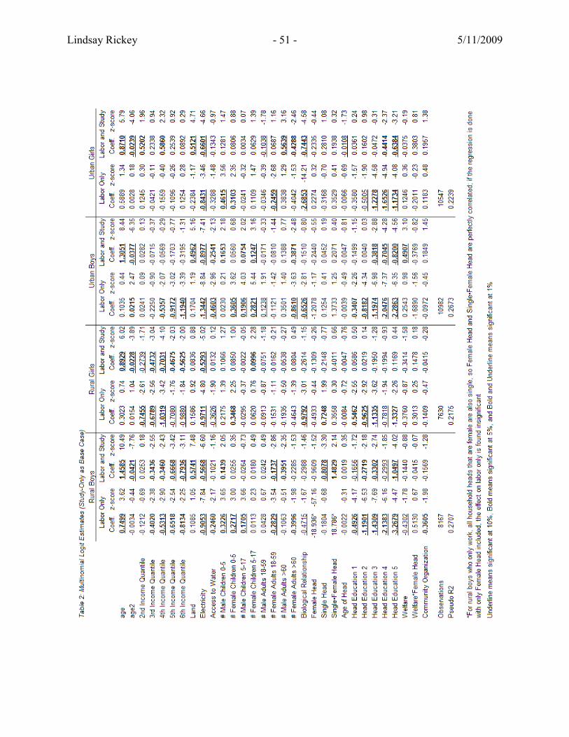
Lindsay Rickey - 51 - 5/11/2009

Lindsay Rickey - 52 - 5/11/2009
6. Conclusions
I have found strong support in the Philippines that income and child labor are correlated.
Programs aimed at promoting economic growth and alleviating poverty should help reduce child
labor and increase school attendance. Equally important though, is community infrastructure—
electricity, water access, schools, public transport. These strongly reduce the probability that
child will be engaged full time in child labor and also increase the probability that a child will
study full time for all groups of children. This is especially important when one considers the
intergenerational effects. Children who grow up to be household heads will be more likely to
allow their children to study full time rather than work if they have more education. If, on the
other hand, children work full time or cannot successfully study in combination with strenuous
labor, their educational level will most likely be the same or worse than their parents. As we can
see from the results, lower education levels lead to more child labor, even when controlling for
household income. If we also assume that less education leads to less income, the negative
effects of working rather than studying will be passed down from generation to generation.
Government welfare programs, on the other hand, seem to do little to alleviate child
labor, probably due to the fact that the poorest are generally unaware of them. Similarly, it
seems that community organizations are generally built in relatively richer areas and hence are
not particularly helpful to the most poverty-stricken. Strengthening government communication
with the poor could make these programs more effective. These results also reveal that children
who do not have a strong biological attachment to the household head are much more likely to
work and less likely to study. This indicates that children in the care of adults that are unrelated
or distantly related are often mistreated compared to biological children. Government programs

Lindsay Rickey - 53 - 5/11/2009
designed to help these children would also reduce the overall incidence of child labor, especially
for urban girls.
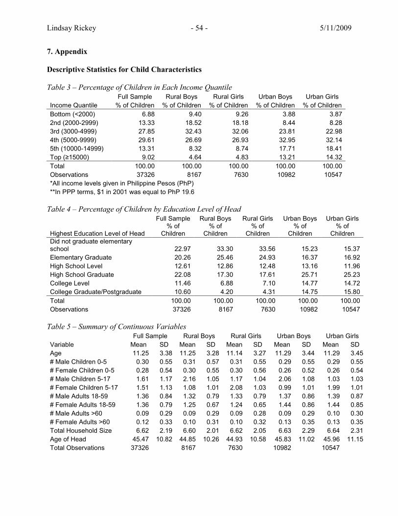
Lindsay Rickey - 54 - 5/11/2009
7. Appendix
Descriptive Statistics for Child Characteristics
Table 3 – Percentage of Children in Each Income Quantile
Full Sample Rural Boys Rural Girls Urban Boys Urban Girls
Income Quantile % of Children % of Children % of Children % of Children % of Children
Bottom (<2000) 6.88 9.40 9.26 3.88 3.87
2nd (2000-2999) 13.33 18.52 18.18 8.44 8.28
3rd (3000-4999) 27.85 32.43 32.06 23.81 22.98
4th (5000-9999) 29.61 26.69 26.93 32.95 32.14
5th (10000-14999) 13.31 8.32 8.74 17.71 18.41
Top (≥15000) 9.02 4.64 4.83 13.21 14.32
Total 100.00 100.00 100.00 100.00 100.00
Observations 37326 8167 7630 10982 10547
*All income levels given in Philippine Pesos (PhP)
**In PPP terms, $1 in 2001 was equal to PhP 19.6
Table 4 – Percentage of Children by Education Level of Head
Full Sample Rural Boys Rural Girls Urban Boys Urban Girls
Highest Education Level of Head % of
Children % of
Children % of
Children % of
Children % of
Children Did not graduate elementary school 22.97 33.30 33.56 15.23 15.37
Elementary Graduate 20.26 25.46 24.93 16.37 16.92
High School Level 12.61 12.86 12.48 13.16 11.96
High School Graduate 22.08 17.30 17.61 25.71 25.23
College Level 11.46 6.88 7.10 14.77 14.72
College Graduate/Postgraduate 10.60 4.20 4.31 14.75 15.80
Total 100.00 100.00 100.00 100.00 100.00
Observations 37326 8167 7630 10982 10547
Table 5 – Summary of Continuous Variables
Full Sample Rural Boys Rural Girls Urban Boys Urban Girls
Variable Mean SD Mean SD Mean SD Mean SD Mean SD
Age 11.25 3.38 11.25 3.28 11.14 3.27 11.29 3.44 11.29 3.45
# Male Children 0-5 0.30 0.55 0.31 0.57 0.31 0.55 0.29 0.55 0.29 0.55
# Female Children 0-5 0.28 0.54 0.30 0.55 0.30 0.56 0.26 0.52 0.26 0.54
# Male Children 5-17 1.61 1.17 2.16 1.05 1.17 1.04 2.06 1.08 1.03 1.03
# Female Children 5-17 1.51 1.13 1.08 1.01 2.08 1.03 0.99 1.01 1.99 1.01
# Male Adults 18-59 1.36 0.84 1.32 0.79 1.33 0.79 1.37 0.86 1.39 0.87
# Female Adults 18-59 1.36 0.79 1.25 0.67 1.24 0.65 1.44 0.86 1.44 0.85
# Male Adults >60 0.09 0.29 0.09 0.29 0.09 0.28 0.09 0.29 0.10 0.30
# Female Adults >60 0.12 0.33 0.10 0.31 0.10 0.32 0.13 0.35 0.13 0.35
Total Household Size 6.62 2.19 6.60 2.01 6.62 2.05 6.63 2.29 6.64 2.31
Age of Head 45.47 10.82 44.85 10.26 44.93 10.58 45.83 11.02 45.96 11.15
Total Observations 37326 8167 7630 10982 10547

Lindsay Rickey - 55 - 5/11/2009
Descriptive Statistics for Child Characteristics (Cont’d)
Table 6 – % of Children (5-17) Who Answered Yes
Full Sample Rural Boys Rural Girls Urban Boys Urban Girls
Male 51.30
Land 28.43 41.40 40.77 18.98 19.30
Rural 42.32
Electricity 77.54 59.13 61.11 90.17 90.53
Access to Water 80.76 71.70 71.04 87.49 87.79
Biological Relation 95.69 97.07 96.74 95.66 93.91
Female Head 10.46 7.97 8.32 12.12 12.21
Single Head 12.41 10.41 10.73 13.74 13.78
Single and Female Head 9.50 7.29 7.65 10.95 11.03
Welfare 6.85 6.47 6.83 6.80 7.21
Welfare and Female Head 0.68 0.47 0.43 0.83 0.86
Community Organization 11.00 11.17 11.22 10.54 11.21
Total Observations 37326 8167 7630 10982 10547
Table 7 – Child Activity
% of Children Engaged in Activity
Child Activity Full Sample Rural Boys Rural Girls Urban Boys Urban Girls
Labor 12.18 21.49 10.55 11.09 7.30
Study 95.86 91.81 97.55 95.84 97.80
Labor Only 4.14 8.19 2.45 4.16 2.20
Study Only 87.82 78.51 89.45 88.91 92.70
Labor and Study 8.05 13.30 8.10 6.93 5.10
Observations 37326 8167 7630 10982 10547

Lindsay Rickey - 56 - 5/11/2009
Child Labor versus Child Work Table 8 - % of Children Engaged in Child Work and Child Labor % of Total Children (5-17)
Child Activity Full Sample Rural Boys Rural Girls Urban Boys Urban Girls
Work 16.05 27.48 15.19 13.85 10.11
Labor 12.18 21.49 10.55 11.09 7.30
Observations 37326 8167 7630 10982 10547
Table 9 - % of Children 5-17 Engaged in Work Defined as Child Labor
% of Working Children (5-17) Who Answered Yes
Hazardous work? 19.74 26.78 13.29 28.40 9.47
In bad conditions? 30.58 32.09 30.37 35.70 35.65
Heavy labor? 26.49 39.39 17.60 34.45 10.88
Stressful? 35.25 44.39 35.81 39.32 27.30 Worked nights often? 20.88 13.73 20.02 27.55 37.80
Observations 6524 2244 1159 1521 1066
Table 10 - % of Children Aged 5-14 Engaged in Work Defined as Child Labor
% of Working Children (5-14) Who Answered Yes Not attending school? 17.91 22.26 9.53 22.59 11.49
>9 hours per day 4.92 4.24 3.78 6.00 6.54
>5 hours/day for >2 days/week
14.88 17.29 8.47 17.57 13.47
Observations 3132 1249 661 717 505
Household Characteristics by Income Level
Table 11 – Household Level Characteristics of Each Income Quantile
Income Quantile # Households % of Total % Own Land % Aware of
Welfare % with Community
Organization
Bottom (<2000) 1200 6.88 28.75 4.25 6.58
2nd (2000-2999) 2325 13.33 30.88 4.95 8.04
3rd (3000-4999) 4859 27.85 28.79 6.36 9.49
4th (5000-9999) 5165 29.61 26.52 7.76 11.66
5th (10000-14999) 2322 13.31 27.39 7.71 12.70
Top (≥15000) 1573 9.02 28.67 8.84 17.55
Total 17444 100.00 28.20 6.84 10.89
*All income levels given in Philippine Pesos (PhP)
**In PPP terms, $1 in 2001 was equal to PhP 19.6
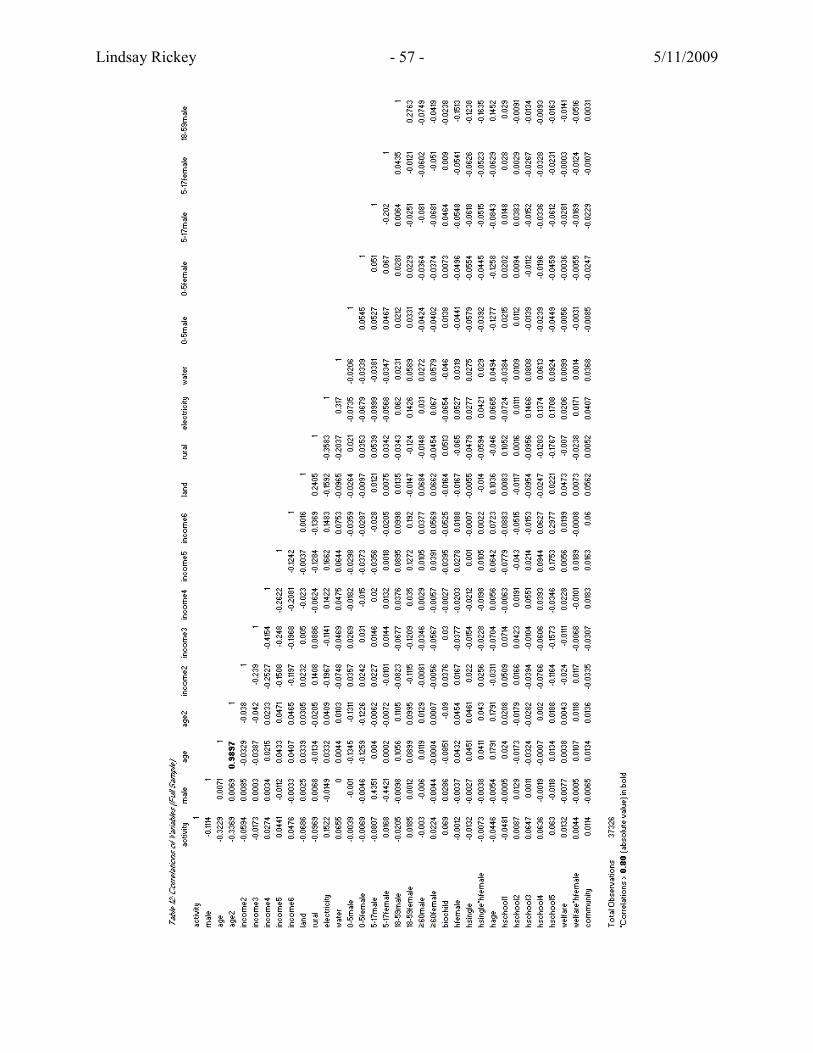
Lindsay Rickey - 57 - 5/11/2009

Lindsay Rickey - 58 - 5/11/2009

Lindsay Rickey - 59 - 5/11/2009

Lindsay Rickey - 60 - 5/11/2009

Lindsay Rickey - 61 - 5/11/2009

Lindsay Rickey - 62 - 5/11/2009

Lindsay Rickey - 63 - 5/11/2009
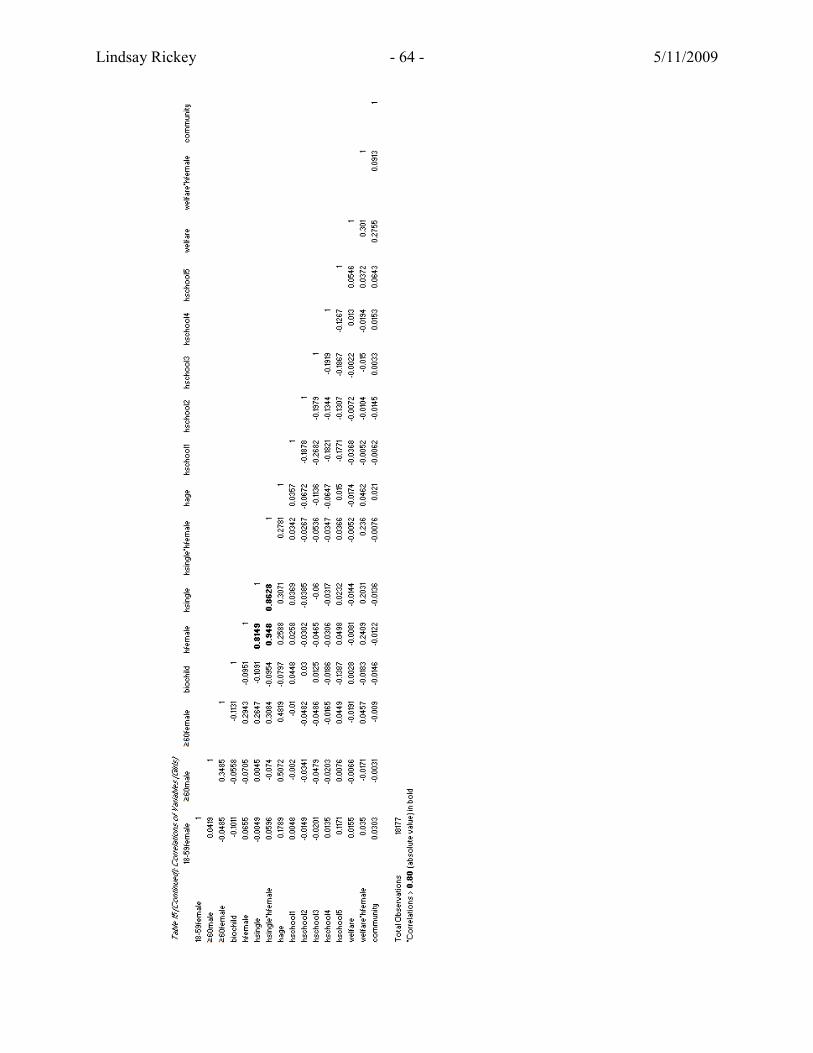
Lindsay Rickey - 64 - 5/11/2009
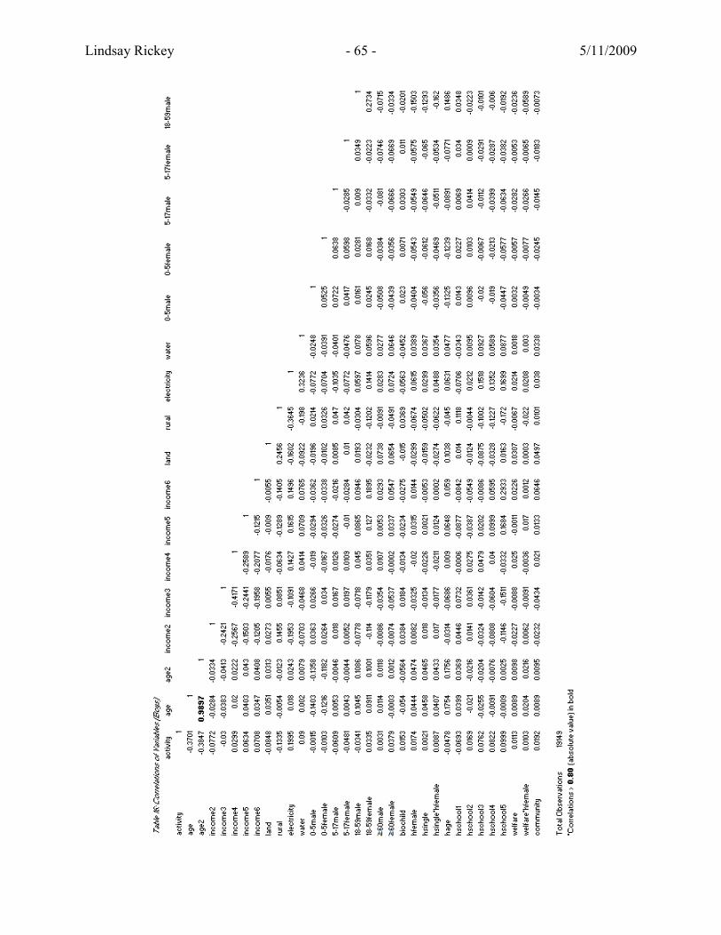
Lindsay Rickey - 65 - 5/11/2009

Lindsay Rickey - 66 - 5/11/2009

Lindsay Rickey - 67 - 5/11/2009

Lindsay Rickey - 68 - 5/11/2009
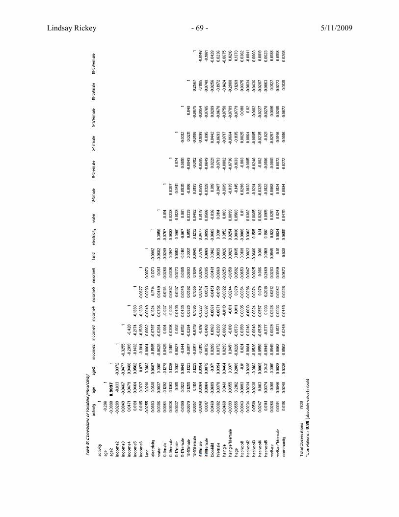
Lindsay Rickey - 69 - 5/11/2009

Lindsay Rickey - 70 - 5/11/2009

Lindsay Rickey - 71 - 5/11/2009

Lindsay Rickey - 72 - 5/11/2009
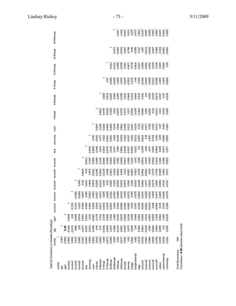
Lindsay Rickey - 73 - 5/11/2009
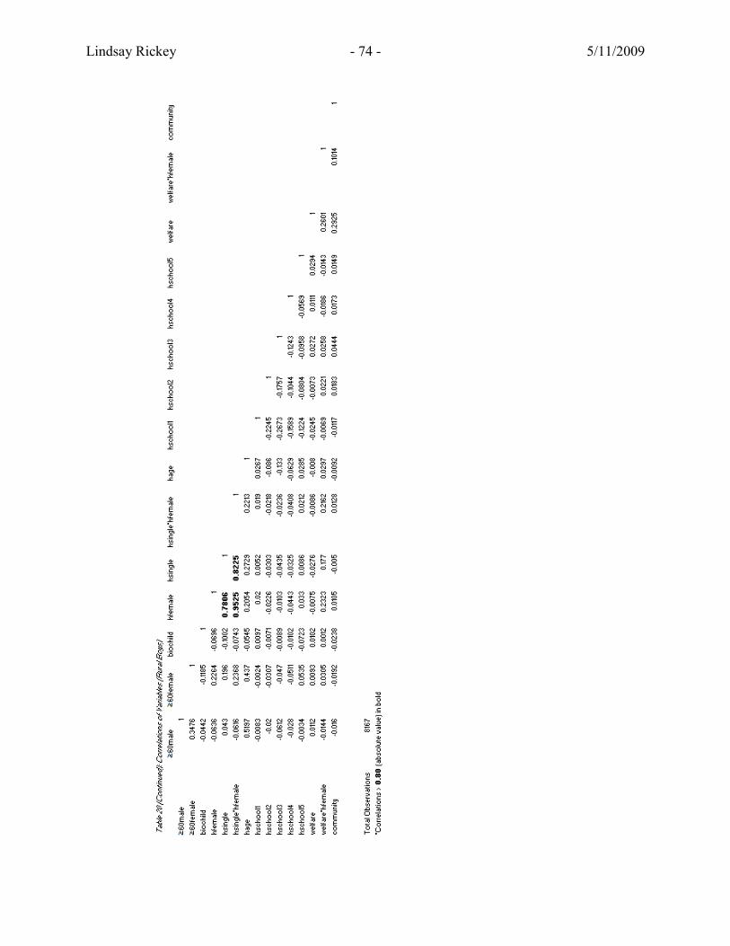
Lindsay Rickey - 74 - 5/11/2009

Lindsay Rickey - 75 - 5/11/2009
8. Reference List
Amin, S., M.S. Quayes and J.M. Rives. 2004. “Poverty and Other Determinants of Child Labor in Bangladesh,” Southern Economic Journal, June 70(4): pp. 876-892.
Basu, Kaushik, and Pham Hoang Van. 1998. “The Economics of Child Labor,” American Economic Review, June 88(3): pp. 412-27.
Behrman, J. and J. Knowles. 1999. “Household Income And Child Schooling In Vietnam,” The World Bank Economic Review, May 13(2): pp. 211-56.
Bhalotra, Sonia and Christopher Heady. 2000. “Child Farm Labor: Theory and Evidence,” London School of Economics. Development and Distribution Series Discussion Paper 24, July.
Bhalotra, Sonia and Christopher Heady. 2003. “Child Farm Labor: The Wealth Paradox,” World Bank Economic Review, 17(2): pp. 197-227.
Bhalotra, Sonia and Zafiris Tzannatos. 2003. “Child Labor: What Have We Learnt?” The World Bank Human Development Network. Social Protection Discussion Paper 0317, September.
Bhatty, Kiran. 1998. “Educational Deprivation in India: A Survey of Field Investigations,” Economic and Political Weekly, July 33(28): pp. 1858-1869.
Bishai, David, El Daw Suliman, Heena Brahmbhatt, Fred Wabwire-Mangen, Godfrey Kigozi, Nelson Sewankambo, David Serwadda, Maria Wawe, and Ron Gray. 2003. “Does Biological Relatedness Affect Survival?” Demographic Research, May 8(9): pp. 261-278.
Blunch, Niels-Hugo and Dorte Verner. 2001. “Revisiting the Link between Poverty and Child Labor: The Ghanaian Experience,” Centre for Labour Market and Social Research. Working Paper 01-03, April.
Bourguignon, F., F. Ferreira and P. Leite. 2002. “Ex-ante Evaluation of Conditional Cash Transfer Programs: the Case of Bolsa Escola,” The World Bank. Policy Research Working Paper Series 2916.
Canagarajah, S. and H.S. Nielsen. 2001. “Child Labor in Africa: A Comparative Study,” Annals of the American Academy of Political and Social Science, May 575, pp. 71-91.
Canagarajah, Sudharshan and Harold Coulombe. 1999. “Child Labor and Schooling in Ghana,” The World Bank. Policy Research Working Paper 1844.
Cardoso, Eliana and Andrea Souza. 2004. “The Impact of Cash Transfers on Child Labor and School Attendance in Brazil,” Vanderbilt University, Working Papers 0407, April.
Cartwright, K. 1999. “Child Labor in Columbia.” In The Policy Analysis of Child Labor: A Comparative Study, ed. C. Grootaert and H.A. Patrinos, 63-102. New York: St. Martin’s Press.

Lindsay Rickey - 76 - 5/11/2009
Cartwright, K. and H.A. Patrinos. 1999. “Child Labor in Urban Bolivia.” In The Policy Analysis of Child Labor: A Comparative Study, ed. C. Grootaert and H.A. Patrinos, 103-130. New York: St. Martin’s Press.
Carvalho, Irineu. 2000. “Household Income as a Determinant of Child Labour and School Enrolment in Brazil: Evidence from a Social Security Reform,” PhD diss. Massachusetts Institute of Technology.
Case, Anne, Christina Paxson, Joseph Ableidinger. 2004. “Orphans in Africa: Parental Death, Poverty, and School Enrollment,” Demography, August 41(3): pp. 483-508.
Cigno, Alessandro & Furio Camillo Rosati. 2000. “Why do Indian Children Work, and is it Bad for Them?” Institute for the Study of Labor (IZA). Discussion Papers No. 115.
Cigno, Alessandro, Furio Camillo Rosati, and Zafiris Tzannatos. 2001. “Child Labor, Nutrition and Education in Rural India: An Economic Analysis of Parental Choice and Policy Options,” The World Bank Human Development Network. Social Protection Discussion Paper No. 0131, December.
Cockburn, J. 2001. “Income Contributions of Child Work in Rural Ethiopia,” Mimeo, University of Laval, October. < http://www.crefa.ecn.ulaval.ca/cahier/0117.pdf>
Coulombe, H. 1998. “Child Labor And Education In Côte d’Ivoire,” The World Bank. Background Paper.
Dayioglu, Meltem. 2006. “The Impact of Household Income on Child Labour in Urban Turkey,” Journal of Development Studies, August 42(6): pp. 939-56.
Deb, Partha, and Furio Camillo Rosati. 2004. “Determinants of Child Labor and School Attendance: The Role of Household Unobservables,” ILO, World Bank, and UNICEF. Understanding Children’s Work Working Paper, April.
Duflo, Esther. 2003. “Grandmothers and Granddaughters: Old-Age Pensions and Intrahousehold Allocation in South Africa,” World Bank Economic Review, 17(1): pp. 1-25.
Dumas, C. 2007. “Why Do Parents Make Their Children Work? A Test of the Poverty Hypothesis in Burkina Faso,” Oxford Economic Papers-New Series, April 59(2): pp. 301-329.
Edmonds, Eric V. 2005. “Does Child Labor Decline with Improving Economic Status?” Journal of Human Resources, Winter 40(1): pp. 77-99.
Edmonds, Eric V. 2006. “Child Labor and Schooling Responses to Anticipated Income in South Africa,” Journal of Development Economics, December 81(2): pp. 386-414.
Emerson, Patrick M. and Andre Souza. 2008. “Birth Order, Child Labor, and School Attendance in Brazil,” World Development, September 36(9): pp. 1647-64.

Lindsay Rickey - 77 - 5/11/2009
Ersado, L. 2005. “Child Labor and Schooling Decisions in Urban and Rural Areas: Comparative Evidence from Nepal, Peru, and Zimbabwe,” World Development, March 33(3): pp. 455-480.
Grootaert, C. 1999. “Child Labor in Côte d’Ivoire: Incidence and Determinants,” The World Bank. Policy Research Working Paper Series No. 1905.
Ilahi, Nadeem. 2001. “Children’s Work and Schooling: Does Gender Matter? Evidence from the Peru LSMS Panel Data,” The World Bank. Policy Research Working Paper No. 2745, December.
International Labour Organization – International Programme on the Elimination of Child Labour (ILO-IPEC). 2004. Child Labour: A Textbook for University Students. Geneva, Switzerland: International Labour Office.
Jensen, Peter and Helena Skyt Nielsen. 1997. “Child Labour or School Attendance? Evidence from Zambia,” Journal of Population Economics, October 10(4): pp. 407-24.
Kruger, Diana I. 2007. “Coffee Production Effects on Child Labor and Schooling in Rural Brazil,” Journal of Development Economics, March 82(2): pp. 448-63.
Liu, A.Y. 1998. “School Children’s Participation Behaviour in Vietnam: An Empirical Analysis,” Paper presented at the Twelfth Annual Conference of the European Society for Population Economics, Amsterdam, Netherlands.
National Statistics Office (NSO) and ILO-IPEC. 2003. 2001 Survey on Children 5-17 Years Old: Final Report. Manila, Philippines: International Labor Office.
Nielsen, H. S. 1998. “Child Labor And Schooling In Zambia,” The World Bank. Working Paper.
Patrinos, H.A. and G. Psacharopoulos. 1995. “Educational Performance and Child labor in Paraguay,” International Journal of Educational Development, 15(1): pp. 47-60.
Patrinos, H.A. and G. Psacharopoulos. 1997. “Family Size, Schooling And Child Labor In Peru - An Empirical Analysis,” Journal of Population Economics, October 10(4): pp. 387-406.
Ravallion, Martin and Quentin T. Wodon. 1999. “Does Child Labor Displace Schooling? Evidence on Behavioral Responses to an Enrollment Subsidy,” The World Bank. Policy Research Working Paper No. 2116, May.
Ray, Ranjan. 1998. “Analysis of Child Labour in Peru and Pakistan: A Comparative Study,” Mimeo, University of Tasmania, Australia.
Ray, Ranjan. 2000. “Child Labour, Child Schooling and their Interaction with Adult Labor: Empirical Evidence for Peru and Pakistan,” The World Bank Economic Review, May 14(2): pp. 347-71.

Lindsay Rickey - 78 - 5/11/2009
Rosati, Furio Camillo and Mariacristina Rossi. 2003. “Children's Working Hours and School Enrollment: Evidence from Pakistan and Nicaragua.” World Bank Economic Review, 17(2): pp. 283-95.
Rosati, Furio Camillo and Zafiris Tzannatos. 2000. “Child Labor In Vietnam,” The World Bank. Working Paper No. 14.
Rosati, Furio Camillo and Zafiris Tzannatos. 2006. “Child Labour in Vietnam,” Pacific Economic Review, 11(1): pp. 1-31.
Rubalcava, Luis, Graciela Teruel, and Duncan Thomas. 2009. “Impacts of the Oportunidades Program: Investments, Time Preferences, and Public Transfers Paid to Women,” Economic Development and Cultural Change, April 57(3): pp. 507-38.
Sakellariou, Chris and Ashish Lall. 1999. “Child Labor in the Philippines.” In The Policy Analysis of Child Labor: A Comparative Study, ed. C. Grootaert and H.A. Patrinos, 131-51. New York: St. Martin’s Press.
Sasaki, M. and T. Temesgen. 1999. “Children in Different Activities: Child Labor and Schooling in Peru,” Mimeo, The World Bank.
Schady, Norbert and Maria Caridad Araujo. 2006. “Cash Transfers, Conditions, School Enrollment, and Child Work: Evidence from a Randomized Experiment in Ecuador,” The World Bank. World Bank Policy Research Working Paper No. 3930, June.
Subbarao, K., A. Mattimore and K. Plangemann. 2001. “Social Protection Of Africa’s Orphans And Vulnerable Children: Issues And Good Practice Program Options,” The World Bank. Africa Region Human Development Working Paper, August.
Tunali, I. 1997. “Young Hands at Work: Child Labor in Turkey,” Mimeo, Koc University.