the determinants of corruption a literature survey … · the determinants of corruption a...
TRANSCRIPT

THE DETERMINANTS OF CORRUPTIONA Literature Survey and New Evidence
Harry Seldadyo∗
Jakob de Haan†
Abstract
This paper examines 70 eonomic and non-economic determinants of corruption. UsingFactor Analysis technique, we generate five new indexes on the basis of these determi-nants. Using Extreme Bound Analysis we examine the robustness of the determinantsas well as the new indexes. We find that one of the generated-indexes, namely regula-tory capacity, is the most robust variable in explaining corruption.
Keywords : corruption, Factor Analysis,Extreme Bounds Analysis
JEL code : P16, D73
Paper Prepared for the 2006 EPCS Conference, Turku, Finland, 20-23 April 2006
∗The Presenter. This paper is not to compete the Knut-Wicksell Prize.†Address of Corresponding Author: Jakob de Haan, Faculty of Economics, University of Groningen,
PO Box 800, 9700 AV Groningen, The Netherlands, tel. 31-50-3633706, fax 31-50-3633720, email:[email protected]
1

”Let’s not mince words ...We need to deal with the causes of corruption”
James Wolfenson(The Economist, 4 June 2005, p. 66.)
1 Introduction
Corruption is the misuse of entrusted authority for private benefit. This phenomenonis usually found in the public sector as it primarily involves government officials.1 Inthe words of Nye (1967, p. 417), it is ”endemic in all governments”. Thus, as widelyrecognized, corruption is probably as old as government itself. According to Glynn etal. (1997, p. 7) ”... no region, and hardly any country, has been immune.”
Corruption affects almost all parts of society. Like a cancer, as argued by Amund-sen (1999, p. 1), corruption ”eats into the cultural, political and economic fabric ofsociety, and destroys the functioning of vital organs”. Transparency International (TI)regards corruption as ”... one of the greatest challenges of the contemporary world. Itundermines good government, fundamentally distorts public policy, leads to the mis-allocation of resources, harms the private sector and private sector development andparticularly hurts the poor.”2 The World Bank (WB) has identified corruption as ”thesingle greatest obstacle to economic and social development. It undermines develop-ment by distorting the rule of law and weakening the institutional foundation on whicheconomic growth depends.”3
Corruption has also attracted attention in the academic arena; not only in eco-nomics, but also in sociology, political science, law, etc. In the words of Andvig (1991,p. 58), it is ”a meeting place for research from the various disciplines of the socialsciences and history”. Thus, research in this subject is basically multi- and inter-disciplinary and includes detailed descriptions of corruption scandals, country cases,and cross-country studies. It also ranges from theoretical models to empirical investi-gations.
During the last two decades, various organizations have collected and publisheddata on corruption. They are drawn from two forms of data sources: poll-based data(primary source) and poll-of-polls-based data (secondary source). Data on corruptionare usually expressed on some scale reflecting the perception of respondents, thereforemost corruption indicators are not about the actual level of corruption, but aboutperceived corruption.
A good example of the first type of data —poll-based data— is the International
1There are, however, also various forms of corruption in the private sector. Bowles (2000) listssome of them including insider trading, collusion in asset valuation, and ’information brokerage’.
2www.transparency.org/speeches/pe carter address.html.3www1.worldbank.org/publicsector/anticorrupt/index.cfm.
2

Country Risk Guide data set covering almost 150 countries since the beginning of the1980s. Meanwhile, the most popular poll-of-polls-based data —the second type ofdata— is perhaps the Transparency International data set, calculated on the basis ofindexes drawn from various corruption surveys around the globe done by a numberof organizations (Lambsdorff, 2000, 2001a, 2002, 2003, and 2004a).4 Recently, theWorld Bank has also produced corruption data as part of a governance index alsousing data collected from various international polls (Kaufmann and Kray, 2002a and2002b; Kaufmann, et al., 1999, 2000, 2003, and 2005; Kaufmann, et al., 1999).5
Updating the surveys of Andvig et al. (2000) and Jain (2001), this paper firstreviews and then extends research on the causes of corruption. The reason is straight-forward. Since corruption deteriorates the performance of nations (Mauro, 1995; Tanziand Davoodi, 1997; Gupta et al., 1998; Lambsdorff, 2001b), the determinants of cor-ruption are of considerable importance. Many possible causes of corruption have beensuggested in the literature and this paper critically examines these causes. The rest ofthis paper is constructed as follows. In section 2 we discuss the concept of corruptionand how to measure it, while in section 3 we review research on the causes of corrup-tion. In section 4 we present the outcomes of our factor analysis, while in section 5we outline our methodology and present new evidence. The last section offers someconcluding comments.
4The complete series is available at www.icgg.org/corruption.index.html.5A series of papers by Daniel Kaufmann and his colleagues at the World Bank since
1999 explains the methodological construction of the index. The complete list is provided inwww.worldbank.org/wbi/governance/wp-governance.html.
3
2 Corruption:
Concept and Measurement
In the Oxford Advanced Learner’s Dictionary (2000, p. 281) corruption is describedas: [1] dishonest or illegal behaviour, especially of people in authority, [2] the act oreffect of making somebody change from moral to immoral standards of behaviour.Thus, corruption includes three important elements, namely morality, behaviour, andauthority. Gould (1991, p. 468) explicitly defines corruption as a moral problem, i.e.,corruption is ”an immoral and unethical phenomenon that contains a set of moralaberrations from moral standards of society, causing loss of respect for and confidencein duly constituted authority”.
However, viewing corruption merely as problems of morality and behaviour tendsto individualize a social phenomenon and to simplify it as only ’good’ or ’bad’ phe-nomenon; thus it ignores the socio-political context of corruption. To exist, corruptionshould be supported by discretionary power, economic rents, and a weak judicial sys-tem (Jain, 2001). Discretionary power relates to authority to design and administerregulations, which, in turn, is accompanied by the presence of economic rents associatedwith power. Meanwhile, a weak judicial system refers to low probability of detectionand penalty. Even in the absence of a moral problem, the combination of rent, power,and a weak (or even failure of the) judicial system is enough for corruption to exist.
How can corruption be measured? Even though there are numerous journalisticaccounts of corruption6 it is still difficult to precisely estimate the extent of corruption.However, some researchers have tried to estimate corruption.7 In their studies, corrup-tion is calculated on the basis of micro level data, like data on infrastructure projectsor data drawn from firm-level surveys. Unfortunately, these data do not enable acomparative analysis. For this purpose, other type of data are available.
There are two basic approaches to measure corruption at the macro level, namely(1) general or target-group perception and (2) incidence of corruptive activities (alsoreferred to as proxy method). The first type of measures reflects the feeling of thepublic or a specific group of respondents (sometimes called experts) concerning the
6For instance in The Guardian (March 26, 2004) Charlotte Denny lists 10 country leaders indicat-ing how much money they made with corruption. In the list there are Mohammed Suharto (Indone-sia, 1967-1998) with $15bn-35bn, Ferdinand Marcos (Philippines, 1972-1986) $5bn-10bn, MobutuSese Seko (Zaire, 1965-1997) $5bn, Sani Abacha (Nigeria, 1993-1998) $2bn-5bn, Slobodan Milose-vic (Serbia, 1972-1986) $1bn, Jean-Claude Duvalier (Haiti, 1971-1986) $300m-800m, Alberto Fuji-mori (Peru, 1990-2000) $600m, Pavlo Lazarenko (Ukraine, 1996-1997) $114m-200m, Arnoldo Alemn(Nicaragua, 1997-2002) $100m, and Joseph Estrada (Philippines, 1998-2001) with $78m-80m. Source:http://www.guardian.co.uk/indonesia/Story/0,2763,1178382,00.html.
7See, for instance, Wade (1982) for the case of India, Murray-Rust and van der Valde (1994) forPakistan, Manzetti and Blake (1996) for Latin America; more recent publications include Svensson(2003) for Uganda, Kuncoro (2004), and Henderson and Kuncoro (2004) for Indonesia, and Goldenand Picci (2005) for Italy.
4
’lack of justice’ in public transactions. Therefore, corruption perception is an indirectmeasure of the actual level of corruption. The incidence-based approach is based onsurveys among those who potentially bribe and those whom bribes are offered. Throughthis approach, a researcher can get information on how frequently corruption occurs invarious types of transactions (The Hungarian Gallup Institute, 2000).8
Golden and Picci (2005) criticize survey-based measures of corruption as they haveat least two intrinsic weaknesses. First, the reliability of survey information aboutcorruption is largely unknown. Respondents directly involved in corruption may haveincentives to underreport such involvement, and those not involved typically lack ac-curate information. Secondly, the reliability of the index may deteriorate over time.There is a danger that respondents report what they believe based on the highly pub-licized results of the most index rather than how much ’real’ corruption exists.
In terms of representative sampling, surveys among the general public may bebetter. However, various respondents may have no experience with corruption. Theirperception may not be very stable over time, since it is highly depending on how muchattention corruption receives in the media. Meanwhile, using specific target groups asthe source of corruption perception can yield maximum information about corruptionalthough not necessarily honestly expressed. The drawback is that these groups maynot be fully representative, being a corruption-prone sub sample of the general public.
Kaufmann and Kraay (2002b) point out that the advantage of a survey among ex-perts is that it is explicitly designed for cross-country comparability. The disadvantageis that such a poll is typically based on the opinions of a few experts per country, andits quality is highly depending on the knowledge of these expert on the countries theyassess. The advantage of surveys among the general public or (foreign) business peopleis that they reflect the opinions of a larger number of people closely connected with thecountries they are assessing. There are also disadvantages of surveys among businesspeople or citizens. First, survey questions can be interpreted in culture-specific ways. Aquestion on ’improper practices’, for example, is certainly coloured by country-specificperceptions of what is meant by ’improper’. Second, such approaches are costly re-sulting in a much smaller set of countries than poll of experts. Furthermore, foreignbusiness people are not accustomed to the local customs and language and tend tooversee the ways how issues are settled locally. As a consequence, their evaluation maybe biased.
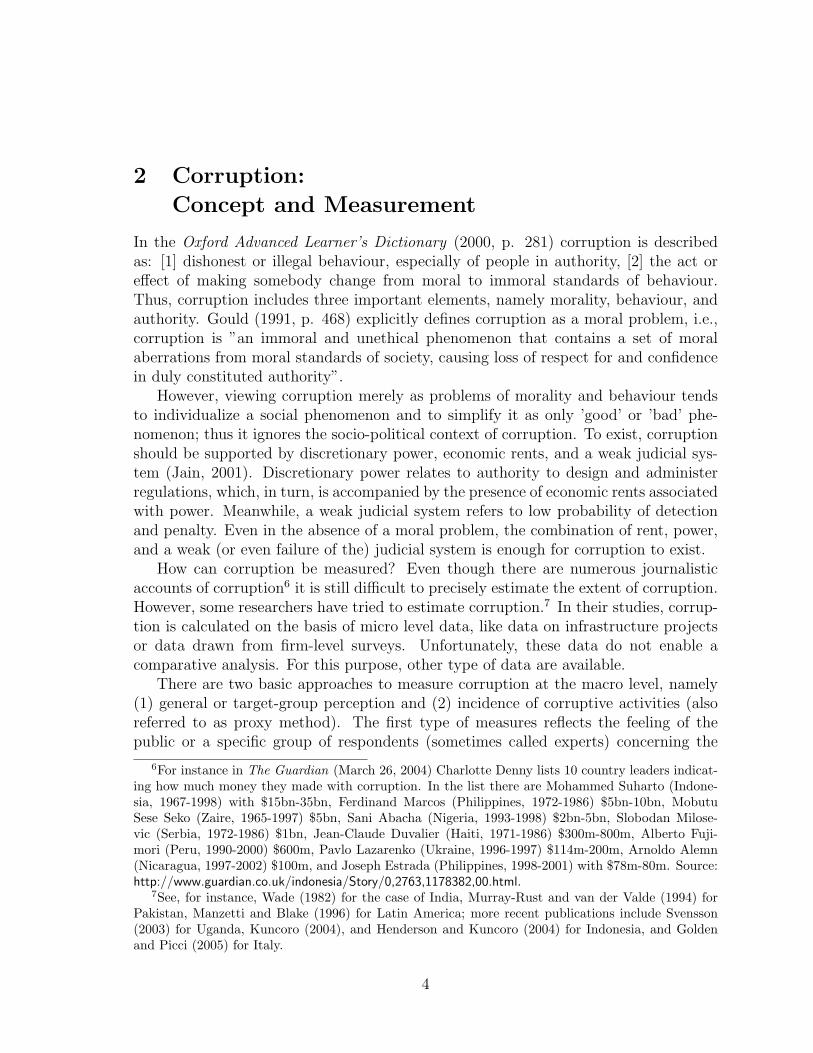
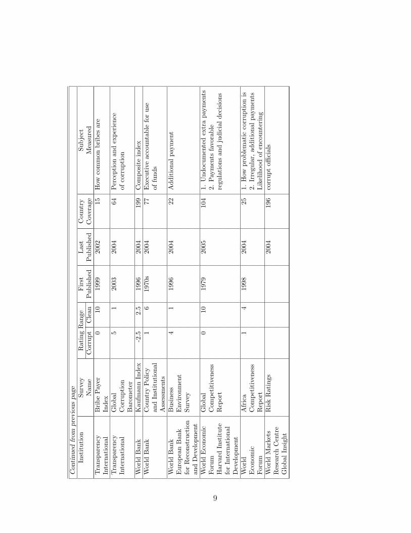
Table 1 summarizes the approaches of various organizations that publish informa-tion on corruption. A quick look at the Table shows that the approaches differ alongfive dimensions. First, corruption is defined in various forms, ranging from bureau-
8We categorize poll- or survey-based measures as ’macro’ level analysis instead of ’micro’ level ofanalysis because of two reasons. First, they are usually directed to generate corruption indexes oncountry-wide basis, not, say, firm-level basis; and these indexes are used for country-level comparison.Second, aggregation methods are usually applied to measure corruption drawn from these polls orsurveys.
5
cratic corruption to political corruption. Second, the indexes fall into two categories:poll-based and poll-of-polls-based indexes. The former generates the indexes from di-rect surveys (perception or proxy method), while the latter combines or aggregatesdata from direct surveys into a single index of corruption. Third, the indexes usedifferent scales of measurement, ranging from qualitative statements to quantitativerating systems. Fourth, some organizations focus on particular regions only —like theones found in Afrobarometer, Asian Intelligence, and Latinobarometro— while othershave a wider coverage of countries, like the surveys done by Political Risk Services-International Country Risk Guide (PRS-ICRG), Standard and Poor’s, etc. Fifth, theinstitutions that publish information on corruption are private firms, multilateral or-ganizations, and non-governmental organizations. As a consequence, some indexesare only provided on a commercial basis, while others are supplied for free.9 In thefollowing, instead of discussing all indexes, we will focus on the mostly used indexes.
9Especially for the comercial-survey-based indexes, choice of countries certainly depends on theattractiveness of the countries in terms of investment, business climate, geopolitical influence, etc.These factors are important for international economic and political decisions.
6

Tab
le1:
Surv
eys
onC
orru
ption
Inst
itut
ion
Surv
eyR
atin
gR
ange
Fir
stLas
tC
ount
rySu
bje
ctN
ame
Cor
rupt
Cle
anP
ublis
hed
Pub
lishe
dC
over
age
Mea
sure
dIn
stit
ute
for
Afr
obar
omet
erPer
cent
age
Per
cent
age
1999
2004
121.
How
com
mon
corr
upti
onD
emoc
racy
inSu
rvey
fair
ly-v
ery
fair
ly-v
ery
amon
gpu
blic
offici
als
Sout
hA
fric
a,co
mm
onra
re2.
Whe
ther
orno
tco
rrup
tion
Gha
naC
entr
ew
orse
unde
rth
eD
emoc
rati
cpr
evio
usre
gim
eD
evel
opm
ent,
Mic
higa
nSt
ate
Uni
vers
ity
Bus
ines
sPol
itic
alR
isk
010
019
70s
2003
50H
owfr
eque
ntly
corr
upti
onE
nvir
onm
enta
lIn
dex
requ
ired
inbu
sine
ssR
isk
Inte
llige
nce
Col
umbi
aSt
ate
Cap
acity
Seve
reLow
1990
2003
95Se
veri
tyof
corr
upti
onU
nive
rsity
Stan
dard
and
Cou
ntry
Ris
k0
1019
9610
6Im
med
iate
and
seco
ndar
yPoo
r’s
DR
IR
evie
wri
skev
ents
Eco
nom
ist
Cou
ntry
Ris
k1
1019
8020
0411
5Per
vasi
vene
ssof
corr
upti
onIn
telli
genc
eU
nit
Free
dom
Nat
ions
in7
119
9520
0327
Lev
elof
corr
upti
onH
ouse
Tra
nsit
ion
Inst
itut
efo
rW
orld
Man
agem
ent
Com
peti
tive
ness
010
1987
2005
60B
ribi
ngan
dco
rrup
tion
Dev
elop
men
tY
earb
ook
inth
epu
blic
sphe
reB
ribi
ngan
dco
rrup
tion
inth
eec
onom
yIm
puls
eE
xpor
ter
Bri
bery
100
1994
103
Pro
port
ion
ofde
alIn
dex
invo
lved
corr
upt
paym
ents
Info
rmat
ion
Surv
eyof
Mid
dle
2004
31H
owco
mm
onbr
ibes
Inte
rnat
iona
lE
aste
rnB
usin
ess
How
cost
lyth
eyfo
rdo
ing
Con
tinued
onnex
tpag
e
7

Con
tinued
from
pre
vio
us
pag
eIn
stit
utio
nSu
rvey
Rat
ing
Ran
geFir
stLas
tC
ount
rySu
bje
ctN
ame
Cor
rupt
Cle
anP
ublis
hed
Pub
lishe
dC
over
age
Mea
sure
dbu
sine
ssH
owfr
eque
ntly
publ
icco
ntra
cts
awar
ded
tofr
iend
san
dre
lati
ves
Inte
rnat
iona
lPol
itic
alR
isk
06
1982
2004
144
Gov
.off
.to
dem
and
Cou
ntry
Ris
ksp
ecia
lpa
ymen
tsG
uide
Ille
galpa
ymen
tsge
nera
llyex
pect
edIn
tern
atio
nal
Cri
me
1989
58G
ov.
off.
toas
kW
orki
ngV
icti
mSu
rvey
topa
ya
brib
efo
rhi
sse
rvic
eG
roup
Lat
inob
arom
etro
Lat
inob
arom
etro
100
019
8820
0317
1.C
orru
ptio
n’in
crea
sed
alo
t’,
Surv
ey’a
littl
e’;’d
ecre
ased
alo
t’’a
littl
e’;or
’rem
aine
dth
esa
me’
the
last
12m
onth
s2.
Dir
ect
expe
rien
ceof
corr
upti
on3.
Pro
port
ion
ofco
rrup
tci
vilse
rvan
tsM
erch
ant
Gre
yA
rea
100
019
90s
2004
155
Ran
gefr
ombr
iber
yof
gov.
min
iste
rsIn
tern
atio
nal
Dyn
amic
sto
indu
cem
ents
paya
ble
toth
eG
roup
’hum
bles
tcl
erk’
Mul
tila
tera
l20
0247
wid
espr
ead
the
inci
denc
eD
evel
opm
ent
ofco
rrup
tion
Ban
kPol
itic
alan
dA
sian
100
1980
s20
0512
1.E
xten
tof
corr
upti
onE
cono
mic
Ris
kIn
telli
genc
e2.
Rat
eof
corr
upti
onin
term
sof
its
Con
sult
ancy
Issu
equ
ality
cont
ribu
tion
toth
eov
eral
lliv
ing/
wor
king
envi
ronm
ent
Pri
ceO
paci
ty15
00
2001
2004
35Fr
eque
ncy
ofco
rrup
tion
Wat
erho
use
Inde
xC
oope
rsTra
nspa
renc
yPer
cept
ion
010
1995
2005
146
Com
posi
tein
dex
Inte
rnat
iona
lIn
dex
Con
tinued
onnex
tpag
e
8
Con
tinued
from
pre
vio
us
pag
eIn
stit
utio
nSu
rvey
Rat
ing
Ran
geFir
stLas
tC
ount
rySu
bje
ctN
ame
Cor
rupt
Cle
anP
ublis
hed
Pub
lishe
dC
over
age
Mea
sure
dTra
nspa
renc
yB
ribe
Pay
er0
1019
9920
0215
How
com
mon
brib
esar
eIn
tern
atio
nal
Inde
xTra
nspa
renc
yG
loba
l5
120
0320
0464
Per
cept
ion
and
expe
rien
ceIn
tern
atio
nal
Cor
rupt
ion
ofco
rrup
tion
Bar
omet
erW
orld
Ban
kK
aufm
ann
Inde
x-2
.52.
519
9620
0419
9C
ompo
site
inde
xW
orld
Ban
kC
ount
ryPol
icy
16
1970
s20
0477
Exe
cuti
veac
coun
tabl
efo
rus
ean
dIn
stit
utio
nal
offu
nds
Ass
essm
ents
Wor
ldB
ank
Bus
ines
s4
119
9620
0422
Add
itio
nalpa
ymen
tE
urop
ean
Ban
kE
nvir
onm
ent
for
Rec
onst
ruct
ion
Surv
eyan
dD
evel
opm
ent
Wor
ldE
cono
mic
Glo
bal
010
1979
2005
104
1.U
ndoc
umen
ted
extr
apa
ymen
tsFo
rum
Com
peti
tive
ness
2.Pay
men
tsfa
vora
ble
Har
vard
Inst
itut
eR
epor
tre
gula
tion
san
dju
dici
alde
cisi
ons
for
Inte
rnat
iona
lD
evel
opm
ent
Wor
ldA
fric
a1
419
9820
0425
1.H
owpr
oble
mat
icco
rrup
tion
isE
cono
mic
Com
peti
tive
ness
2.Ir
regu
lar,
addi
tion
alpa
ymen
tsFo
rum
Rep
ort
Lik
elih
ood
ofen
coun
teri
ngW
orld
Mar
kets
Ris
kR
atin
gs20
0419
6co
rrup
toffi
cial
sR
esea
rch
Cen
tre
Glo
balIn
sigh
t
9
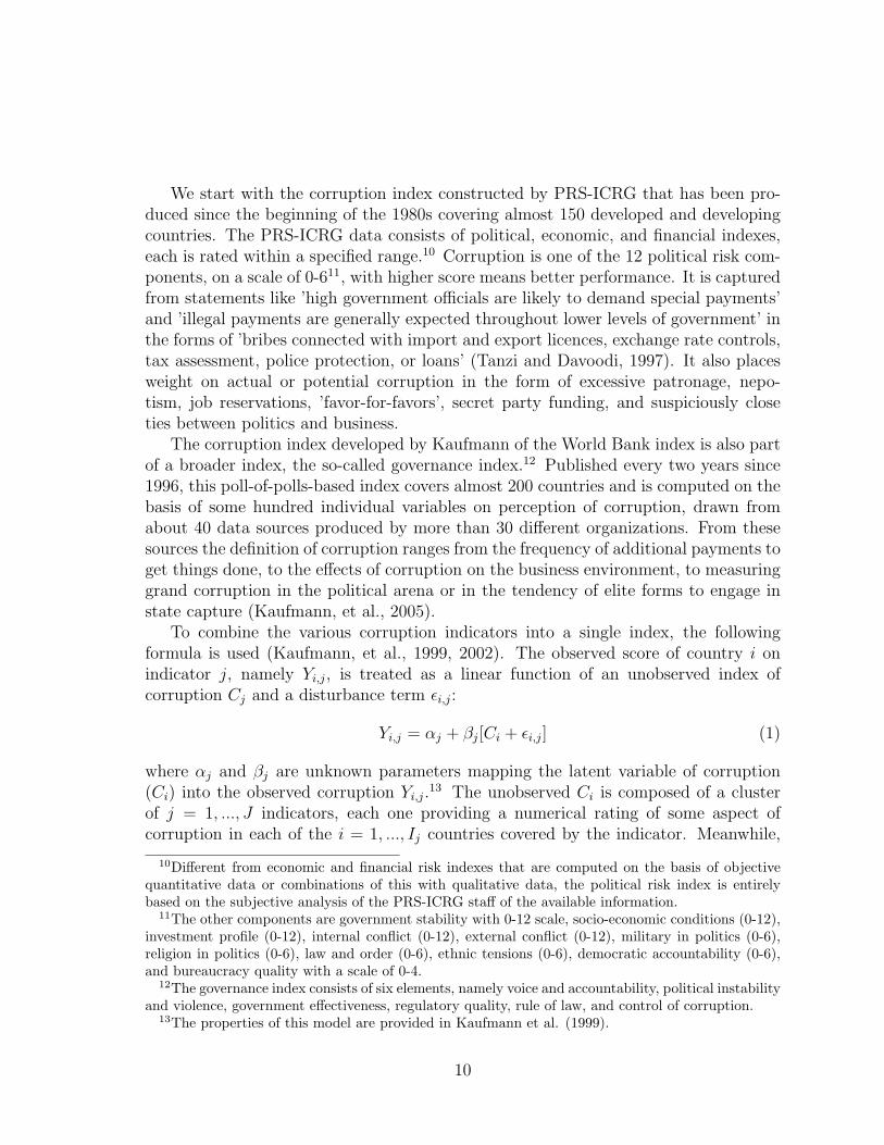
We start with the corruption index constructed by PRS-ICRG that has been pro-duced since the beginning of the 1980s covering almost 150 developed and developingcountries. The PRS-ICRG data consists of political, economic, and financial indexes,each is rated within a specified range.10 Corruption is one of the 12 political risk com-ponents, on a scale of 0-611, with higher score means better performance. It is capturedfrom statements like ’high government officials are likely to demand special payments’and ’illegal payments are generally expected throughout lower levels of government’ inthe forms of ’bribes connected with import and export licences, exchange rate controls,tax assessment, police protection, or loans’ (Tanzi and Davoodi, 1997). It also placesweight on actual or potential corruption in the form of excessive patronage, nepo-tism, job reservations, ’favor-for-favors’, secret party funding, and suspiciously closeties between politics and business.
The corruption index developed by Kaufmann of the World Bank index is also partof a broader index, the so-called governance index.12 Published every two years since1996, this poll-of-polls-based index covers almost 200 countries and is computed on thebasis of some hundred individual variables on perception of corruption, drawn fromabout 40 data sources produced by more than 30 different organizations. From thesesources the definition of corruption ranges from the frequency of additional payments toget things done, to the effects of corruption on the business environment, to measuringgrand corruption in the political arena or in the tendency of elite forms to engage instate capture (Kaufmann, et al., 2005).
To combine the various corruption indicators into a single index, the followingformula is used (Kaufmann, et al., 1999, 2002). The observed score of country i onindicator j, namely Yi,j, is treated as a linear function of an unobserved index ofcorruption Cj and a disturbance term εi,j:
Yi,j = αj + βj[Ci + εi,j] (1)
where αj and βj are unknown parameters mapping the latent variable of corruption(Ci) into the observed corruption Yi,j.
13 The unobserved Ci is composed of a clusterof j = 1, ..., J indicators, each one providing a numerical rating of some aspect ofcorruption in each of the i = 1, ..., Ij countries covered by the indicator. Meanwhile,
10Different from economic and financial risk indexes that are computed on the basis of objectivequantitative data or combinations of this with qualitative data, the political risk index is entirelybased on the subjective analysis of the PRS-ICRG staff of the available information.
11The other components are government stability with 0-12 scale, socio-economic conditions (0-12),investment profile (0-12), internal conflict (0-12), external conflict (0-12), military in politics (0-6),religion in politics (0-6), law and order (0-6), ethnic tensions (0-6), democratic accountability (0-6),and bureaucracy quality with a scale of 0-4.
12The governance index consists of six elements, namely voice and accountability, political instabilityand violence, government effectiveness, regulatory quality, rule of law, and control of corruption.
13The properties of this model are provided in Kaufmann et al. (1999).
10
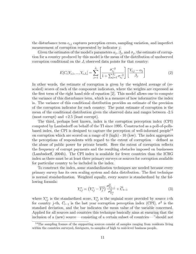
the disturbance term εi,j captures perception errors, sampling variation, and imperfectmeasurement of corruption represented by indicator j.
Given the estimates of the model’s parameters αj, βj, and σj, the estimate of corrup-tion for a country produced by this model is the mean of the distribution of unobservedcorruption conditional on the Ji observed data points for that country:
E[Ci|Yi,1, ..., Yi,Ji] =
Ji∑j=1
[σ−2
εj
1 +∑Ji
j=1 σ−2εj
] [Yi,j − αj
βj
](2)
In other words, the estimate of corruption is given by the weighted average of (re-scaled) scores of each of the component indicators, where the weights are expressed asthe first term of the right hand side of equation [2]. This model allows one to computethe variance of this disturbance term, which is a measure of how informative the indexis. The variance of this conditional distribution provides an estimate of the precisionof the corruption indicator for each country. The point estimate of corruption is themean of the conditional distribution given the observed data and ranges between -2.5(most corrupt) and +2.5 (least corrupt).
The third, perhaps best known, index is the corruption perception index (CPI)computed by Lambsdorff on behalf of the TI since 1995. Constructed as a poll-of-polls-based index, the CPI is designed to capture the perception of well-informed people14
on corruption which are scored on a range of 0 (high) - 10 (low). The index aggregatesthe perceptions of respondents with regard to the extent of corruption —defined asthe abuse of public power for private benefit. Here the extent of corruption reflectsthe frequency of corrupt payments and the resulting obstacles imposed on businesses(Lambsdorff, 2004b). The CPI index is available for fewer countries than the ICRGindex as there must be at least three primary surveys or sources for corruption availablefor particular country to be included in the index.
To construct the index, some standardization techniques are needed because everyprimary survey has its own scaling system and data distribution. The first techniqueis normal standardization. Weighted equally, every source is standardized by the fol-lowing formula:
Y si,j =
(Y o
i,j − Y oj
) σ2Ct−1
σ2Y o
j
+ Ct−1 (3)
where Y si,j is the standardized score, Y o
i,j is the orginial score provided by source i-thfor country j-th, Ct−1 is the last year corruption perception index (CPI), σ2 is thestandard deviation, and the bar indicates the mean value of the variable concerned.Applied for all sources and countries this technique basically aims at ensuring that theinclusion of a (new) source —consisting of a certain subset of countries— ”should not
14The sampling frames of the supporting sources consist of samples ranging from residents livingwithin the countries surveyed, foreigners, to samples of high to mid-level business people.
11
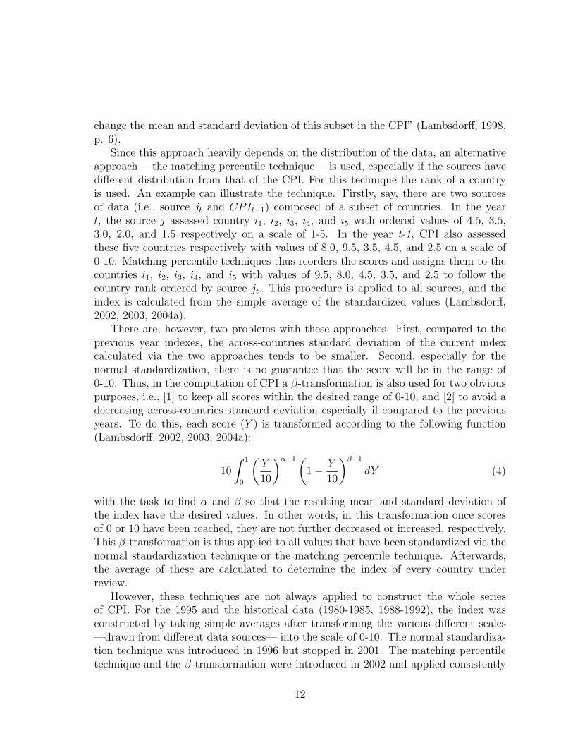
change the mean and standard deviation of this subset in the CPI” (Lambsdorff, 1998,p. 6).
Since this approach heavily depends on the distribution of the data, an alternativeapproach —the matching percentile technique— is used, especially if the sources havedifferent distribution from that of the CPI. For this technique the rank of a countryis used. An example can illustrate the technique. Firstly, say, there are two sourcesof data (i.e., source jt and CPIt−1) composed of a subset of countries. In the yeart, the source j assessed country i1, i2, i3, i4, and i5 with ordered values of 4.5, 3.5,3.0, 2.0, and 1.5 respectively on a scale of 1-5. In the year t-1, CPI also assessedthese five countries respectively with values of 8.0, 9.5, 3.5, 4.5, and 2.5 on a scale of0-10. Matching percentile techniques thus reorders the scores and assigns them to thecountries i1, i2, i3, i4, and i5 with values of 9.5, 8.0, 4.5, 3.5, and 2.5 to follow thecountry rank ordered by source jt. This procedure is applied to all sources, and theindex is calculated from the simple average of the standardized values (Lambsdorff,2002, 2003, 2004a).
There are, however, two problems with these approaches. First, compared to theprevious year indexes, the across-countries standard deviation of the current indexcalculated via the two approaches tends to be smaller. Second, especially for thenormal standardization, there is no guarantee that the score will be in the range of0-10. Thus, in the computation of CPI a β-transformation is also used for two obviouspurposes, i.e., [1] to keep all scores within the desired range of 0-10, and [2] to avoid adecreasing across-countries standard deviation especially if compared to the previousyears. To do this, each score (Y ) is transformed according to the following function(Lambsdorff, 2002, 2003, 2004a):
10
∫ 1
0
(Y
10
)α−1 (1 − Y
10
)β−1
dY (4)
with the task to find α and β so that the resulting mean and standard deviation ofthe index have the desired values. In other words, in this transformation once scoresof 0 or 10 have been reached, they are not further decreased or increased, respectively.This β-transformation is thus applied to all values that have been standardized via thenormal standardization technique or the matching percentile technique. Afterwards,the average of these are calculated to determine the index of every country underreview.
However, these techniques are not always applied to construct the whole seriesof CPI. For the 1995 and the historical data (1980-1985, 1988-1992), the index wasconstructed by taking simple averages after transforming the various different scales—drawn from different data sources— into the scale of 0-10. The normal standardiza-tion technique was introduced in 1996 but stopped in 2001. The matching percentiletechnique and the β-transformation were introduced in 2002 and applied consistently
12

since then.15 As a consequence, the CPI is not a consistent time series. In Lambsdorff’swords, ”... year-to-year changes may not only result from a changing performance of acountry ... changes can result from the different methodologies ... not necessarily fromactual changes.” (Lambsdorff, 2000, p. 4). Apart from changes in the methodology, achange of the CPI for a particular country may also reflect a change in the number ofprimary sources available for this country (Johnston 2001b).
Other criticisms have been raised as well. Galtung (2005) argues that the definitionof corruption in the CPI does not explicitly distinguish between corruption in differentbranches of civil service nor corruption in political party financing. Likewise, Johnston(2001b) notes that the definition is skewed to a form of bribery. Andvig (2005) questionswhether the different sources to form the CPI cover the same phenomenon.16
Since it relies heavily on independently conducted surveys and expert polls, theCPI is not available for a significant number of countries. Its reliance on other sourcesimplies that countries may drop out of the index if the required minimum numberof sources is missing. Galtung (2005) therefore concludes that CPI does not measuretrends. ”The CPI’s principal flaw is that it is a defective and misleading benchmarkof trends” (p. 12).
Despite all these criticisms, it must be recognized that perception-based indexeshave opened the possibility to study corruption empirically as they have made theimmeasurable concept measurable. As a result, numerous studies have employed suchindexes. In the following section we will systematically review empirical studies on thecauses of corruption.
15We received this information from personal communication with Lambsdorff, since there is notechnical explanation for the indexes produced before 1998 and no clear explanation found in theLambsdorff’s Framework Document series.
16Likewise, Soreide (2003, p. 7) argues that ”Most of the polls and surveys ask for a generalimpression of the magnitude of the problem, which actually means people’s subjective intuitions ofthe extent of a hidden activity. For the TI index, only one source asks for people’s personal experienceswith corruption. The quantification of the problem is highly ambiguous. It is not clear to what extentthe level of corruption reflects the frequency of corrupt acts, the severity to society, the size of the bribesor the benefits obtained. Most of the surveys do not specify what they mean by the word corruption.It can thus be quite difficult for the respondents to answer when asked about a quantification of ’themisuse of public office for private or political party gain’ or when encouraged to rate ’the severity ofcorruption within the state’.”
13
3 Empirical Determinants of Corruption
Many studies have searched for empirical regularities between corruption and a varietyof economic and non-economic determinants. Unfortunately, there is no commonly-agreed-upon theory on which to base an empirical model of the causes of corruption(Alt and Lassen, 2003). At the same time, numerous regression models incorporatinga wide variety of explanatory variables have been specified to explain corruption andto find the ’true’ determinants. It is often found that, however, a variable is significantin a particular specification of the model, but loses its significance when some othervariables are incorporated. In other words, claims concerning the determinants ofcorruption are conditional, and the robustness of the findings is open to question.
While other categorizations are possible, we identify four broad classes of underlyingcauses of corruption, namely (1) economic and economic institutions, (2) political,(3) judicial and bureaucratic, and (4) religious and geo-cultural factors. Tables 2-5summarize all studies that we are aware of, indicating the main results concerning thesignificance of the variables belonging to the classes of variables that we distinguish.
3.1 Economic Determinants
Economic factors consist of a wide range of economic variables like income or economicpolicy variables; included here are also demographic variables and economic institu-tions. To start with, we observe that income is a commonly-used variable to explaincorruption (Damania et al., 2004; Persson et al., 2003; and van Rijckeghem and Weder,1997; among others). Mostly proxied by GDP per capita, income is used to controlfor structural differences as economic development progresses. It can be generally con-cluded that a country’s wealth is a significant predictor of corruption, even thoughKaufmann et al. (1999) and Hall and Jones (1999) question the causal relationshipbetween corruption and income. Two studies with panel data (Braun and Di Tella,2004; Frechette, 2001) deviate from this main result, finding that income increasescorruption, especially when they impose fixed effects.
Income distribution is also argued to affect corruption. As Paldam (2002) putsit, ”A skew income distribution may increase the temptation to make illicit gains”.Proxied by the Gini coefficient, he claims that income disparity significantly increasescorruption. However, using the income share of top 20% of the population under adifferent specification, Park (2003) does not find a statistically significant relationship.Similarly, Brown et al. (2005) find no evidence that greater income inequality increasecorruption.
The size of government is also an important source of corruption. If countries exploiteconomies of scale in the provision of public services —thus have a low ratio of publicservice outlets per capita— those who demand the services might be tempted to bribe,e.g., ’to get ahead of the queue’. However, a large government sector may also create
14
opportunities for corruption; that is, the larger the relative size of the public sector,the greater the likelihood of corrupt behaviour. Thus, there is no consensus amongauthors on the theoretical relationship between government size and corruption. Thisis also reflected in the empirical studies of Fisman and Gatti (2002) and Bonaglia etal. (2001) that end up with a different conclusion than the ones of Ali and Isse (2003).Whereas the former finds the negative impact of government spending on corruption,the latter reports the positive impact.
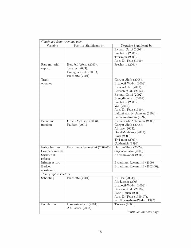
Another variable that according to various authors also explains corruption is im-port share. Herzfeld and Weiss (2003) and Treisman (2000) report that a higher importshare leads to less corruption. A high import share implies lower tariff and non-tariffimport restrictions. The presence of such restrictions —like the necessary licenses toimport, for example— offers an opportunity to bribe. Likewise, a high export share ofraw materials, such as fuel, mineral, and ore, increases the probability of corruptionto occur. Since such endowments create rents, this thus exhibits the phenomenon ofrents-related corruption which is, according to Tornell and Lane (1998), commonlyfound in natural-resource-abundant countries.
In line with the above-mentioned argument, restrictions on foreign trade, foreigninvestment, and capital markets stimulate corruption; see, for example, Knack andAzfar (2003), and Frechette (2001). Likewise, economic freedom —measured by theindexes of the Heritage Foundation/Wall Street Journal and the Fraser Institute— isalso found to lessen corruption. Proponents of this view are Gurgur and Shah (2005),Park (2003), and Treisman (2000), but Lederman et al. (2005) and Paldam (2001)find more mixed results. Broadman and Recanatini (2000, 2002) show the existenceof a positive relationship between entry barriers and corruption; that is, the greaterthe barriers to entry and exit faced by firms, and therefore the greater the distortionsexisting in the competitive environment, the more widespread is corruption.
Finally, we turn to socio-demographic factors associated with corruption. These in-clude schooling, population, and the labour force. Economies with high human capitalhave low levels of corruption as found in Ali and Isse (2003), Brunetti and Weder (2003),and van Rijckeghem and Weder (1997). However, a counter-intuitive finding is foundin Frechette (2001). Using panel data models with fixed effects, he finds that schoolingis positive in all regressions explaining corruption. Similar conflicting evidence is foundfor a country’s population. Knack and Azfar (2003) show that as population increases,corruption also rises, while Tavares (2003) reports that population negatively affectscorruption.
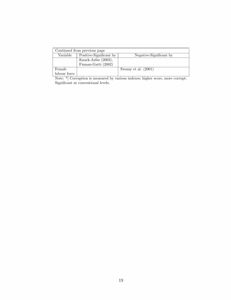
Another interesting demographic variable is the percentage of female population inthe labour force. Swamy et al. (2001) indicate that a higher female labour participationleads to less corruption. Combined with two other gender variables, namely proportionof women in parliament and in government, they find that more influence of womenleads to less corruption. Following Gottfredson and Hirshi (1990) and Paternoster and
15

Simpson (1996), Swamy et al. provide four arguments to explain this finding. First,”women may be brought up to be more honest or more risk averse than men, or evenfeel there is a greater probability of being caught.” Second, ”women, who are typicallymore involved in raising children, may find they have to practice honesty in order toteach their children the appropriate values.” Third, ”women may feel more than men-the physically stronger sex, that laws exist to protect them and therefore be morewilling to follow rules.” Lastly, ”girls may be brought up to have higher levels ofself-control than boys which affects their propensity to indulge in criminal behaviour.”
16
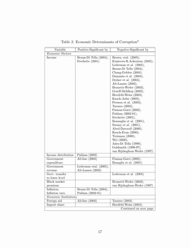
Table 2: Economic Determinants of Corruption*
Variable Positive-Significant by Negative-Significant byEconomic FactorsIncome Braun-Di Tella (2004), Brown, etal. (2005),
Frechette (2001) Kunicova-R.Ackerman (2005),Lederman et al. (2005),Braun-Di Tella (2004),Chang-Golden (2004),Damania et al. (2004),Dreher et al. (2004),Alt-Lassen (2003),Brunetti-Weder (2003),Graeff-Mehlkop (2003),Herzfeld-Weiss (2003),Knack-Azfar (2003),Persson et al. (2003),Tavares (2003),Fisman-Gatti (2002),Paldam (2002-01),Frechette (2001),Bonanglia et al. (2001),Swamy et al. (2001),Abed-Davoodi (2000),Rauch-Evan (2000),Treisman (2000),Wei (2000),Ades-Di Tella (1999),Goldsmith (1999-97),van Rijckeghem-Weder (1997)
Income distribution Paldam (2002)Government Ali-Isse (2003) Fisman-Gatti (2002),expenditure Bonaglia et al. (2001)Government Lederman etal. (2005),revenue Alt-Lassen (2003)Govt. transfer Lederman et al. (2005)to lower levelBlack market Brunetti-Weder (2003),premium van Rijckeghem-Weder (1997)Inflation, Braun-Di Tella (2004),Inflation vars. Paldam (2002-01)Economic InstitutionsForeign aid Ali-Isse (2003) Tavares (2003)Import share Herzfeld-Weiss (2003),
Continued on next page
17
Continued from previous pageVariable Positive-Significant by Negative-Significant by
Fisman-Gatti (2002),Frechette (2001),Treisman (2000),Ades-Di Tella (1999)
Raw material Herzfeld-Weiss (2003), Frechette (2001)export Tavares (2003),
Bonaglia et al. (2001),Frechette (2001)
Trade Gurgur-Shah (2005),opennes Brunetti-Weder (2003),
Knack-Azfar (2003),Persson et al. (2003),Fisman-Gatti (2002),Bonaglia et al. (2001),Frechette (2001),Wei (2000),Ades-Di Tella (1999),Laffont and N’Guessan (1999),Leite-Weidmann (1997)
Economic Graeff-Mehlkop (2003), Kunicova-R.Ackerman (2005),freedom Paldam (2001) Gurgur-Shah (2005),
Ali-Isse (2003),Graeff-Mehlkop (2003),Park (2003),Treisman (2000),Goldsmith (1999)
Entry barriers, Broadman-Recanatini (2002-00) Gurgur-Shah (2005),Competitiveness Suphacahlasai (2005)Structural Abed-Davoodi (2000)reformInfrastructure Broadman-Recanatini (2000)Budget Broadman-Recanatini (2002-00),constraintDemographic FactorsSchooling Frechette (2001) Ali-Isse (2003),
Alt-Lassen (2003),Brunetti-Weder (2003),Persson et al. (2003),Evan-Rauch (2000),Ades-Di Tella (1999-97),van Rijckeghem-Weder (1997)
Population Damania et al. (2004), Tavares (2003)Alt-Lassen (2003),
Continued on next page
18
Continued from previous pageVariable Positive-Significant by Negative-Significant by
Knack-Azfar (2003),Fisman-Gatti (2002)
Female Swamy et al. (2001)labour forceNote: *] Corruption is measured by various indexes; higher score, more corrupt.Significant at conventional levels.
19
3.2 Political Determinants
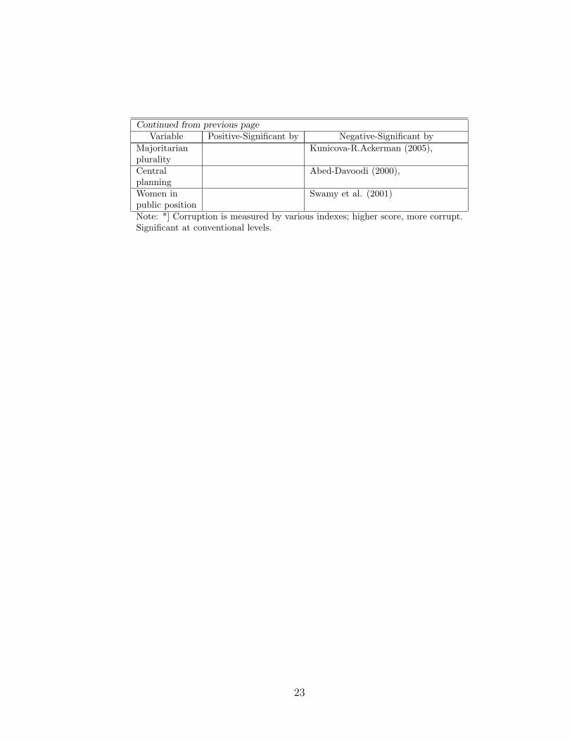
Empirical studies on the political causes of corruption can be divided into two broadgroups, namely those investigating the impact of political-civil liberty and those ex-amining the effect of decentralization on corruption. Meanwhile, other factors thatalso have been suggested to affect corruption are the electoral system (Persson et al.,2003; Kunicova and Rose-Ackerman, 2005), governmental administration (Brown etal., 2005; Chang and Golden, 2004), and political instability (Park, 2003).
Although various proxies like civil liberty, political freedom, political rights, lengthof democratic regime, etc, have been used, there is a consensus that democracy reducescorruption. This conclusion is confirmed if corruption is related to other democracy-related variables, like freedom of the press. This variable is found to be significantlycorrelated with corruption (Brunetti and Weder, 2003).
The main reason why political liberty tends to reduce corruption is that politicalliberty imposes transparency and provides checks and balances within the politicalsystem. Political participation, political competition, and constraints on the chiefexecutive increase the ability of the population to monitor and legally limit politiciansfrom engaging in corrupt behaviour (Kunicova and Rose-Ackerman, 2005). In addition,it is often found that democratic systems are politically more stable. It is thereforenot surprising that authors like Lederman et al. (2005), Park (2003), and Leite andWeidmann (1997) find that that corruption increases in unstable polities.17
Some aspects of democratic elections may, however, create opportunities for corrup-tion. Selecting politicians through party lists, for example, can obscure the direct linkbetween voters and politicians, thus degrading the ability of voters to hold politiciansaccountable (Kunicova and Rose-Ackerman, 2005; Persson and Tabellini, 2003). Changand Golden (2004), in their study on electoral systems and corruption, find that underopen-list proportional representation increases in district size leads to more corruption.Meanwhile, under closed-list proportional representation arrangements, political cor-ruption becomes less prevalent as district magnitude increases. Similar results are alsofound by Persson et al. (2003).
Decentralization or federalism has also been argued to be crucial to combat corrup-tion, but the empirical evidence is mixed. Measuring decentralization as transfers fromcentral government to other levels of national government as a percentage of GDP, Le-derman et al. (2005) find that this variable reduces corruption significantly. Likewise,taking a binary variable of centralized unitary states and decentralized federal systems,Ali and Isse (2003) report that decentralized government lowers corruption. Gurgurand Shah (2005) use the ratio of employment in non-central government administra-tion to general civilian government employment and show that corruption is lower in
17Another explanation can also be found in Shleifer and Vishny (1993) who pose that the ephemeralnature of public positions in unstable systems makes officials irresponsible and get them involved inillicit rent-seeking behaviour.
20
both decentralized unitary and federal states but the impact is higher in decentralizedunitary system. Fisman and Gatti (2002) measure decentralization as the sub-nationalshare of total government spending. The numerator is the total expenditure of subnational (state and local) governments, while the denominator is total spending by alllevels (state, local, and central) of government. They find the negative effect of fiscaldecentralization on corruption, even after controlling for potential joint endogeneity.
In contrast, Kunicova and Rose-Ackerman (2005) using a simple dummy for au-tonomous regions with extensive taxing, spending and regulatory authority argue thatfederalism increases corruption, holding other factors constant. Likewise, using adummy variable for the presence of a federal constitution, Damania et al. (2004) andTreisman (2000) find that a federal structure is more conducive to corruption. ”As thepolitical pie is divided between a greater number of geographic entities, opportunitiesto generate political rents increase” (Brown et al., 2005, p. 12). Similarly, Goldsmith(1999) also demonstrates that federalism is associated with more perceived corruption.
21

Table 3: Political and Political Institution Determinants of Corruption*
Variable Positive-Significant by Negative-Significant byDemocracy, Kunicova-R.Ackerman (2005),civil liberty Lederman et al. (2005),
Gurgur-Shah (2005),Braun-Di Tella (2004),Chang-Golden (2004),Damania et al. (2004),Herzfeld-Weiss (2003),Knack-Azfar (2003),Broadman-Recanatini (2002-00),Paldam (2002),Bonaglia et al. (2001),Frechette (2001),Swamy etal. (2001),Treisman (2000),Wei (2000),Ades-Di Tella (1999-97),Leite-Weidmann (1997),Goldsmith (1999),van Rijckeghem-Weder (1997)
Press freedom, Lederman et al. (2005),Media Suphacahlasai (2005),
Brunetti-Weder (2003)Decentralization, Brown et al. (2005), Gurgur-Shah (2005),federalism Kunicova-R.Ackerman (2005), Lederman etal. (2005),
Damania et al. (2004), Fisman-Gatti (2002),Treisman (2000), Ali-Isse (2003),Goldsmith (1999) Wei (2000)
District maginute Chang-Golden (2004)Closed list Kunicova-R.Ackerman (2005), Lederman et al. (2005),system Persson-Tabellini (2003), Chang-Golden (2004)
Persson et al (2003),Presidentialism Brown, et al. (2005),
Kunicova-R.Ackerman (2005),Lederman et al. (2005),Chang-Golden (2004)
Number of Chang-Golden (2004)partyPolitical Park (2003),instability Leite-Weidmann (1999)Ideological Brown, et al. (2005),Polarization
Continued on next page
22
Continued from previous pageVariable Positive-Significant by Negative-Significant by
Majoritarian Kunicova-R.Ackerman (2005),pluralityCentral Abed-Davoodi (2000),planningWomen in Swamy et al. (2001)public positionNote: *] Corruption is measured by various indexes; higher score, more corrupt.Significant at conventional levels.
23

3.3 Bureaucratic and Regulatory Determinants
The judicial system and the quality of bureaucracy are crucial factors influencing cor-ruption. In this context, the wage level of civil servants may be important, since —asargued by van Rijckeghem and Weder (1997)— public sector wages are highly corre-lated with the measures of the rule of law and the quality of the bureaucracy, andtherefore may have an effect on corruption. In developing economies bureaucrats re-ceive wages that are so low to entice corrupt behaviour. At the same time, low incomeeconomies suffer from the lack of institutions for detecting corruption. Measured as therelative magnitude of wage to GDP, Herzfeld and Weiss (2003) identify that an increasein wages significantly lessens corruption. Similary, van Rijckeghem and Weder (1997)claim that government wages as the ratio to manufacturing wages significantly reducescorruption. The influence wage on corruption is also highlighted by Alt and Lassen(2003) and Rauch and Evans (2000). However, other studies reveal that this relation-ship is not always to be statistically significant (Gurgur and Shah, 2005; Treisman,2000).
Gurgur and Shah (2005), Brunetti and Weder (2003), and van Rijckeghem andWeder (1997) report that the higher the quality of bureaucracy, the lower the prob-ability for corruption to occur. Along with this finding, it is also interesting to seethat the lack of meritocratic recruitment and promotion and the absence of profes-sional training in the bureaucracy are also found to be associated with high corruption(Rauch and Evans, 1997).
Finally, various studies suggest that the rule of law, proxied by various measures,is relevant in explaining corruption. Damania et al. (2004) use the rule of law indexof Kaufmann et al. (1999a,b) that takes several indicators into account to measurethe extent to which economic agents abide by the rules of society, perceptions of theeffectiveness and predictability of the judiciary, and the enforceability of contracts. Agroup of authors (Brunetti and Weder, 2004; Ali and Isse, 2003; Herzfeld and Weiss,2003; Park 2003; and Leite and Weidmann, 1999) use the ICRG index to reflect the de-gree to which the citizens of a country are willing to accept the established institutionsto make and implement laws and adjudicate disputes. This index also measures theextent to which countries have sound political institutions, strong courts, and orderlysuccession of power. All these authors claim that a strong rule of law reduces the like-lihood of corruption to take place. This result is significant under various regressionspecifications.
24
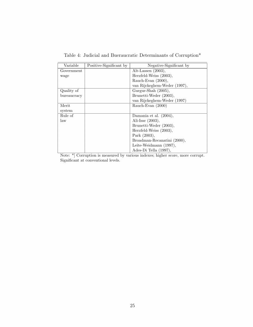
Table 4: Judicial and Bueraucratic Determinants of Corruption*
Variable Positive-Significant by Negative-Significant byGovernment Alt-Lassen (2003),wage Herzfeld-Weiss (2003),
Rauch-Evan (2000),van Rijckeghem-Weder (1997),
Quality of Gurgur-Shah (2005),bureaucracy Brunetti-Weder (2003),
van Rijckeghem-Weder (1997)Merit Rauch-Evan (2000)systemRule of Damania et al. (2004),law Ali-Isse (2003),
Brunetti-Weder (2003),Herzfeld-Weiss (2003),Park (2003),Broadman-Recanatini (2000),Leite-Weidmann (1997),Ades-Di Tella (1997),
Note: *] Corruption is measured by various indexes; higher score, more corrupt.Significant at conventional levels.
25

3.4 Geographical, Cultural, and Religious Determinants
Religion, culture, and geography may also matter for explaining corruption. Countrieswith many Protestants tend to have lower corruption levels (Chang and Golden, 2004;Bonaglia et al., 2001; Treisman, 2000; La Porta et al., 1999). Paldam (2001) reportsthat countries dominated by two religions, namely Reform Christianity (e.g., Protestantand Anglican) and Tribal religions, tend to have lower levels of corruption comparedto countries in which other religions dominate.
As to cultural variables, many authors find that ethno-linguistic homogeneity tendsto reduce corruption (Lederman et al., 2005; La Porta et al., 1999). This finding isexplained in terms of the increased difficulties that bureaucrats encounter in extractingbribes from ethnic groups to which he does not belong. The domination of an ethnicgroup in a country generates an unequal access to power. Minorities with less politicalaccess thus collude with bureaucrats for levelling the political and economic landscape.In ethnically diverse communities, a bureaucrat behaves sequentially: first to his closekin, to his ethnic group, and then maybe to his country (Ali and Isse, 2003). As aresult, highly fragmented communities are likely to be more corrupt than homogenoussocieties.
Another cultural variable used to explain corruption is colonial heritage that cap-tures ’command and control habits and institutions and the divisive nature of thesociety left behind by colonial masters’ (Gurgur and Shah, 2005, p. 18). The evidenceon the relevance of this variable is, however, mixed. Countries that have been colonial-ized tend to suffer from corruption (Gurgur and Shah, 2005; Tavares, 2003). Herzfeldand Weiss (2003), on the other hand, find that former British colonies have lower levelsof corruption. Persson et al. (2003) measure the influence of colonial history by parti-tioning all former colonies into three groups, namely British, Spanish-Portuguese, andother colonial origin, and define three binary indicator variables for these groups. Theyfind that former British colonies tend to have a lower current propensity for corruption.
26

Table 5: Cultural and Geographical Determinants of Corruption*
Variable Positive-Significant by Negative-Significant byPop. with Paldam (2001), Chang-Golden (2004),particular La Porta et al (1999) Herzfeld-Weiss (2003),religious Persson et al. (2003),affiliation Bonaglia et al. (2001),
Paldam (2001),Treisman (2000),La Porta et al (1999)
Ethnic Lederman et al (2005), Bonaglia et al.(2001)heterogeneity Suphachalasai (2005),
Herzfeld-Weiss (2003),Treisman (2000),La Porta et al (1999)
Colonial Gurgur-Shah (2005) Herzfeld-Weiss (2003),past Tavares (2003) Persson et al. (2003),
Swamy et al. (2001),Treisman (2000)
Distance to Ades-Di Tella (1999) Bonaglia et al.(2001),large exporterLegal Gatti (1999), Suphachalasai (2005),origin La Porta et al (1999)Area wide Bonaglia et al.(2001),Latitude La Porta et al (1999),Mascullinity Park (2003)Natural Leite-Weidmann (1997)resourcesNote: *] Corruption is measured by various indexes; higher score, more corrupt.Significant at conventional levels.
27
4 Data Imputation and Factor Analysis
The main objective of this paper is to rexamine the claims of the above-mentionedauthors on the significance of the corruption determinants in various corruption regres-sions. We do regression analysis on these determinants by taking Kaufmann corruptionindex 2004 (corka04) as the dependent variable. As the literature suggests a long listof variables causing corruption, we have collected as many variables as possible thathave been suggested determining corruption. Table 6 presents the variables we havecollected and their sources, while table 7 provides the statistical summary of them.
Since the total number of explanatory variables is huge, no doubt multicollinear-ity will become a problem in our regression analysis. Some variables, however, canpossibly be clustered into some groups representing a particular phenomena. The sec-ond problem is that not all data are available for the same set of countries. We haveonly a few variables capturing all 193 country samples, namely GDP per capita, pop-ulation density, and country area; for the other variables the number of observationsvaries from 52 to 191. This implies that we have missing data problem. To deal withthe first problem, we use Exploratory Factor Analysis (EFA) to reduce the number ofexplanatory variables. However, we first solve the missing data problem.
The question of how to treat incomplete data is among the most complicated prob-lems faced by policy analysts. Because of the lack of data, the degree of uncertaintyincreases with the level of data aggregation and influences the ability to draw accurateconclusions. We minimize the degree of uncertainty using the data imputation tech-nique of Expectation-Maximization (EM) as suggested by Dempster, et al. (1977) andRuud (1991). The EM algorithm is basically an iterative method that can be dividedinto two stages. First, in the ’expectation’ stage, we form a log-likelihood function forthe latent data as if they were observed and taking its expectation. Second, in the’maximization’ stage, the resulting expected log-likelihood is maximized.
Prior to the imputation we transform all variables to improve the distributionalcharacteristics of the data.18 A more normal (symmetric) distribution implies that themajority of data fall within the two standard deviations of the mean and extreme valuesoccur with small probability. If the observed minimum of the variable is negative, weadd a constant such that the transformation of negative values can be computed (seeTable 7).
18Before the transformation, variables like economic freedom of Heritage Foundation and pressfreedom are rescaled to give them the same interpretation as the other variables. Thus higher valuesmean more freedom. The same rescaling is applied for corruption and the other Kaufmann indexes ofgovernance.
28

Tab
le6:
The
Var
iable
s
No
Var.
Definit
ion
Year
Sourc
e
1cork
a04
contr
olofcorr
upti
on
(-2.5
:corr
upt;
+2.5
:cle
an);
Reori
ente
d2004
worl
dbank.o
rg/w
bi/
govern
ance/pdf/
2004kkdata
.xls
2gdpcap
per
capit
agdp
at
const
ant
pri
ces
inU
Sdollars
2000
gdp:
unst
ats
.un.o
rg/unsd
/sn
aam
a/dow
nlo
ads/
GD
Pconst
antU
S-c
ountr
ies.
xls
2000
popula
tion:
devdata
.worl
dbank.o
rg/edst
ats
/query
/defa
ult
.htm
3gin
igin
iin
dex
1993-2
000
Hum
an
Develo
pm
ent
Indic
ato
r2005
4ri
ch10
the
richest
10%
ofpopula
tion
1993-2
000
Hum
an
Develo
pm
ent
Indic
ato
r2005
5ri
ch20
the
richest
20%
ofpopula
tion
1993-2
000
Hum
an
Develo
pm
ent
Indic
ato
r2005
6govcon
share
ofgenera
lgovern
ment
finalconsu
mpti
on
expendit
ure
2000
unst
ats
.un.o
rg/unsd
/sn
aam
a/dow
nlo
ads/
Share
s-countr
ies.
xls
7aid
cap
aid
per
capit
a(c
urr
ent
US$)
2000
devdata
.worl
dbank.o
rg/data
-query
/8
debtg
ni
tota
ldebt
per
gni
2000
rroja
sdata
bank.o
rg/dev0000.h
tm9
totd
ebt
totd
ebt
(000000)
2000
nati
onm
ast
er.
com
/gra
ph-T
/eco
deb
ext
cap
10
debtg
dp
debt
per
gdp
(00)
2000
nati
onm
ast
er.
com
/gra
ph-T
/eco
deb
ext
gdp
11
mpor
share
ofim
port
sofgoods
and
serv
ices
unst
ats
.un.o
rg/unsd
/sn
aam
a/dow
nlo
ads/
Share
s-countr
ies.
xls
12
xpor
share
ofexport
sofgoods
and
serv
ices
unst
ats
.un.o
rg/unsd
/sn
aam
a/dow
nlo
ads/
Share
s-countr
ies.
xls
13
xfu
el
export
offu
el(%
tota
lm
erc
handis
eexport
)2000
WD
I2002
14
xm
eta
lexport
ofore
sand
meta
l(%
tota
lm
erc
handis
eexport
)2000
WD
I2002
15
are
a1
size
ofgovern
ment,
frase
r,(0
:lo
west
freedom
;10:
hig
hest
freedom
)2000
freeth
ew
orl
d.c
om
./2005/2005D
ata
set.
xls
16
are
a2ab
judic
ialin
dependence-im
part
ialcourt
,fr
ase
r,(0
:lo
west
freedom
;10:
hig
hest
freedom
)2000
freeth
ew
orl
d.c
om
./2005/2005D
ata
set.
xls
17
are
a3
sound
money,fr
ase
r,(0
:lo
west
freedom
;10:
hig
hest
freedom
)2000
freeth
ew
orl
d.c
om
./2005/2005D
ata
set.
xls
18
are
a4b
freedom
totr
ade
inte
rnati
onally,fr
ase
r,(0
:lo
west
freedom
;10:
hig
hest
freedom
)2000
freeth
ew
orl
d.c
om
./2005/2005D
ata
set.
xls
19
are
a5b
labor
regula
tion,fr
ase
r,(0
:lo
west
freedom
;10:
hig
hest
freedom
)2000
freeth
ew
orl
d.c
om
./2005/2005D
ata
set.
xls
20
efh
eri
tecon.
freedom
ofheri
tage
found.(
1:
hig
hest
freedom
;5:
low
est
freedom
):R
eori
ente
d2000
heri
tage.o
rg/re
searc
h/fe
atu
res/
index/dow
nlo
ads.
cfm
21
open
share
ofim
port
+export
sofgoods
and
serv
ices
2000
unst
ats
.un.o
rg/unsd
/sn
aam
a/dow
nlo
ads/
Share
s-countr
ies.
xls
22
enro
lpgro
ssenro
llm
ent
rate
(%,pri
mary
school)
2000
devdata
.worl
dbank.o
rg/edst
ats
/query
/defa
ult
.htm
23
enro
lsgro
ssenro
llm
ent
rate
(%,se
condary
school)
2000
devdata
.worl
dbank.o
rg/edst
ats
/query
/defa
ult
.htm
24
enro
ltgro
ssenro
llm
ent
rate
(%,te
rtia
rysc
hool)
2000
devdata
.worl
dbank.o
rg/edst
ats
/query
/defa
ult
.htm
25
illi
Est
imate
dillite
racy
rate
and
illite
rate
popula
tion
aged
15
years
and
old
er
2000
uis
.unesc
o.o
rg/T
EM
PLAT
E/htm
l/Excelt
able
s/educati
on/
Vie
wTable
Lit
era
cy
Countr
yA
ge15+
.xls
26
popden
popula
tion
per
km
sq.
are
a2000
27
fem
lab
fem
ale
labor
forc
e(%
ofto
tal)
2000
devdata
.worl
dbank.o
rg/edst
ats
/query
/defa
ult
.htm
28
pr
politi
calri
ght
(1:
hig
hest
freedom
;7:
low
est
freedom
)2000
freedom
house
.org
/ra
tings/
index.h
tm29
cl
civ
illibert
y(1
:hig
hest
freedom
;7:
low
est
freedom
)2000
freedom
house
.org
/ra
tings/
index.h
tm30
poli
index
auto
cra
cy-d
em
ocra
cy
(-10:
auto
cra
tic;+
10:
dem
ocra
tic)
2000
cid
cm
.um
d.e
du/in
scr/
polity
/polr
eg.h
tm31
dem
ac
dem
ocra
tic
accounta
bility
(1-6
:hig
her
score
bett
er
perf
orm
ance)
2000
icrg
32
voic
voic
eaccounta
bility
(-2.5
-+
2.5
:hig
her
score
bett
er
perf
orm
ance)
2000
worl
dbank.o
rg/w
bi/
govern
ance/pdf/
2004kkdata
.xls
33
pre
sspre
ssfr
eedom
(0:
hig
hest
freedom
;100:
low
est
freedom
);R
eori
ente
d2000
freedom
house
.org
/re
searc
h/pre
ssurv
ey.h
tm34
snexg
Sub-N
ati
onalG
overn
ment
Expendit
ure
(%gdp)
govern
ment
financia
lst
ati
stic
s35
snre
gSub-N
ati
onalG
overn
ment
Revenue
(%gdp)
govern
ment
financia
lst
ati
stic
s36
snexe
Sub-N
ati
onalG
overn
ment
Expendit
ure
(%to
talgovt.
expend.)
govern
ment
financia
lst
ati
stic
s37
snre
rSub-N
ati
onalG
overn
ment
Revenue
(%to
talgovt.
revenue)
govern
ment
financia
lst
ati
stic
s38
dis
tmag
mean
dis
tric
tm
agnit
ude
(House
):avera
ge
no.
ofle
gis
lato
rs2000
site
reso
urc
es.
worl
dbank.o
rg/IN
TR
ES/R
eso
urc
es/
ele
cte
dto
the
low
er
house
from
each
dis
tric
tD
PI2
004-n
ofo
rmula
no
macro
.xls
39
pre
siden
Dir
ect
Pre
sidenti
al(0
);st
rong
pre
sident
ele
cte
dby
ass
em
bly
(1);
Parl
iam
enta
ry(2
)2000
site
reso
urc
es.
worl
dbank.o
rg/IN
TR
ES/R
eso
urc
es/
DPI2
004-n
ofo
rmula
no
macro
.xls
40
pst
apoliti
calst
ability
(-2.5
-+
2.5
:hig
her
score
bett
er
perf
orm
ance)
2000
worl
dbank.o
rg/w
bi/
govern
ance/pdf/
2004kkdata
.xls
41
gst
agovern
ment
stability
(1-1
2:
hig
her
score
bett
er
perf
orm
ance)
2000
icrg
42
inco
inte
rnalconflic
t(1
-12:
hig
her
score
bett
er
perf
orm
ance)
2000
icrg
43
exco
exte
rnalconflic
t(1
-12:
hig
her
score
bett
er
perf
orm
ance)
2000
icrg
44
ete
neth
nic
tensi
on
(1-6
:hig
her
score
bett
er
perf
orm
ance)
2000
icrg
45
pola
riz
Maxim
um
pola
rizati
on
betw
een
the
executi
ve
part
yand
the
four
pri
ncip
lepart
ies
ofth
ele
gis
latu
re;
2000
site
reso
urc
es.
worl
dbank.o
rg/IN
TR
ES/R
eso
urc
es/
Conti
nued
on
nex
tpage
29

Conti
nued
from
pre
vio
us
page
No
Var.
Definit
ion
Year
Sourc
eA
lso,th
em
axim
um
diff
ere
nce
betw
een
the
chie
fexecuti
ves
part
ys
valu
eD
PI2
004-n
ofo
rmula
no
macro
.xls
and
the
valu
es
ofth
eth
ree
larg
est
govern
ment
part
ies
and
the
larg
est
opposi
tion
part
y46
plu
ralty
Ele
cto
ralru
le:
Plu
rality
?(1
ifyes,
Oif
no)
2000
site
reso
urc
es.
worl
dbank.o
rg/IN
TR
ES/R
eso
urc
es/
DPI2
004-n
ofo
rmula
no
macro
.xls
47
wage
Tota
lC
entr
algov’t
wage
bill(%
ofG
DP)
1996-2
000
ww
w1.w
orl
dbank.o
rg/publicse
cto
r/civ
ilse
rvic
e/develo
pm
ent.
htm
48
buqua
bure
aucra
tic
quality
(1-4
:hig
her
score
bett
er
perf
orm
ance)
2000
icrg
49
geff
govern
ment
effecti
veness
(-2.5
-+
2.5
:hig
her
score
bett
er
perf
orm
ance)
2000
worl
dbank.o
rg/w
bi/
govern
ance/pdf/
2004kkdata
.xls
50
rlaw
rule
ofla
w(-
2.5
-+
2.5
:hig
her
score
bett
er
perf
orm
ance)
2000
worl
dbank.o
rg/w
bi/
govern
ance/pdf/
2004kkdata
.xls
51
regqua
regula
tory
quality
(-2.5
-+
2.5
:hig
her
score
bett
er
perf
orm
ance)
2000
worl
dbank.o
rg/w
bi/
govern
ance/pdf/
2004kkdata
.xls
52
law
or
law
and
ord
er
(1-4
:hig
her
score
bett
er
perf
orm
ance)
2000
icrg
53
budha
%popula
tion
2005
worl
dchri
stia
ndata
base
.org
/54
hin
du
%popula
tion
2005
worl
dchri
stia
ndata
base
.org
/55
musl
im%
popula
tion
2005
worl
dchri
stia
ndata
base
.org
/56
nonre
lig
%popula
tion
2005
worl
dchri
stia
ndata
base
.org
/57
anglic
%popula
tion
2005
worl
dchri
stia
ndata
base
.org
/58
cath
ol
%popula
tion
2005
worl
dchri
stia
ndata
base
.org
/59
indepen
%popula
tion
2005
worl
dchri
stia
ndata
base
.org
/60
marg
inal
%popula
tion
2005
worl
dchri
stia
ndata
base
.org
/61
ort
hodox
%popula
tion
2005
worl
dchri
stia
ndata
base
.org
/62
pro
test
%popula
tion
2005
worl
dchri
stia
ndata
base
.org
/63
eth
noa
the
pro
bability
that
two
random
lyse
lecte
din
div
iduals
from
the
countr
yin
quest
ion
1960-8
0A
nnett
,A
nth
ony.
2001.
Socia
lFra
cti
onalizati
on,
willnot
belo
ng
toth
esa
me
eth
nic
gro
up.
Politi
calIn
stability,and
the
Siz
eofG
overn
ment.
IMF
48(3
).H
igher
valu
ere
flects
agre
ate
rdegre
eoffr
acti
onalizati
on.
imf.org
/Exte
rnal/
Pubs/
FT
/st
affp/2001/03/annett
.htm
.;hum
andevelo
pm
ent.
bu.e
du/use
exsi
stin
gin
dex/
show
aggre
gate
.cfm
?in
dex
id=
234&
data
type=
164
eth
nob
Avera
ge
valu
eoffive
diff
ere
nt
indic
es
ofeth
onolinguis
tic
fracti
onalizati
on.
La
Port
aet.
al(1
999)
=La
Port
aet.
al(1
998)
Its
valu
era
nges
from
0to
1.
The
five
com
ponent
indic
es
are
:(1
)in
dex
ofeth
nolinguis
tic
fracti
onalizati
on
in1960,w
hic
hm
easu
res
the
pro
bability
that
two
random
lyse
lecte
dpeople
from
agiv
en
countr
yw
illnot
belo
ng
toth
esa
me
eth
nolinguis
tic
gro
up
(the
index
isbase
don
the
num
ber
and
size
ofpopula
tion
gro
ups
as
dis
tinguis
hed
by
their
eth
nic
and
linguis
tic
statu
s);
(2)
pro
bability
oftw
ora
ndom
lyse
lecte
din
div
iduals
speakin
gdiff
ere
nt
languages;
(3)
pro
bability
oftw
ora
ndom
lyse
lecte
din
div
iduals
do
not
speak
the
sam
ela
nguage;
(4)
perc
ent
ofth
epopula
tion
not
speakin
gth
eoffi
cia
lla
nguage;and
(5)
perc
ent
ofth
epopula
tion
not
speakin
gth
em
ost
wid
ely
use
dla
nguage.
65
englis
legalori
gin
La
Port
aet.
al(1
999)
=La
Port
aet.
al(1
998)
66
socia
lle
galori
gin
La
Port
aet.
al(1
999)
=La
Port
aet.
al(1
998)
67
french
legalori
gin
La
Port
aet.
al(1
999)
=La
Port
aet.
al(1
998)
68
germ
an
legalori
gin
La
Port
aet.
al(1
999)
=La
Port
aet.
al(1
998)
69
scandi
legalori
gin
La
Port
aet.
al(1
999)
=La
Port
aet.
al(1
998)
70
lati
tula
titu
de
La
Port
aet.
al(1
999)
=La
Port
aet.
al(1
998)
71
are
akm
land
and
wate
rare
a(k
msq
)cia
.gov/cia
/publicati
ons/
factb
ook/
30

Tab
le7:
Tra
nsf
orm
atio
nan
dIm
puta
tion
No.
Var
iabl
eB
efor
eIm
puta
tion
Tra
nsf.
Con
st.
Aft
erIm
puta
tion
Obs
.M
ean
Std.
Dev
.M
in.
Max
Obs
.M
ean
Std.
Dev
.M
in.
Max
.C
orru
ptio
n1
cork
a04
193
0.02
1.02
-2.5
01.
65sq
.12
.50
193
0.05
1.02
-2.5
01.
68E
cono
mic
Det
erm
inan
ts2
gdpc
ap19
364
03.1
010
651.
6182
.01
7731
9.59
log
019
364
03.1
010
651.
6182
.01
7731
9.59
3gi
ni12
440
.18
10.4
024
.70
70.7
0sr
.0
193
40.4
88.
6024
.70
70.7
04
rich
1012
219
.03
17.6
84.
5087
.20
inv.
019
316
.76
14.4
24.
5087
.18
5ri
ch20
124
10.4
09.
183.
4057
.60
in.s
q.rt
.0
193
9.76
7.47
3.40
57.6
06
govc
on19
30.
180.
130.
031.
07lo
g0
193
0.18
0.13
0.03
1.07
7ai
dcap
159
59.4
713
3.18
0.00
1105
.00
log
019
353
.02
125.
460.
5711
05.0
08
debt
gni
128
83.7
986
.40
2.84
726.
13lo
g0
193
69.5
575
.66
2.84
726.
139
totd
ebt
142
2751
3.04
8453
8.45
10.0
086
8500
.00
log
019
328
982.
9287
381.
1010
.00
8684
97.1
010
debt
gdp
141
27.5
031
.02
0.19
215.
15lo
g0
193
24.9
127
.01
0.19
215.
1511
mpo
r18
80.
500.
380.
003.
62sq
.rt.
019
30.
500.
380.
003.
6212
xpor
191
0.46
0.40
0.00
4.15
sq.r
t.0
193
0.46
0.39
0.00
4.15
13xf
uel
106
17.3
627
.55
0.00
100.
00sq
.rt.
019
314
.05
21.2
40.
0010
0.00
14xm
etal
109
6.17
11.7
60.
0067
.00
sq.r
t.0
193
5.35
9.05
0.00
67.0
015
area
112
25.
751.
502.
299.
19id
ent.
019
35.
801.
212.
299.
1916
area
2ab
122
5.83
1.91
1.98
9.62
log
019
35.
541.
761.
989.
6217
area
312
27.
611.
871.
259.
83sq
.0
193
7.52
1.58
1.25
9.83
18ar
ea4b
121
6.91
1.28
1.66
9.78
sq.
019
36.
751.
141.
669.
7819
area
5b12
25.
881.
062.
718.
35sq
.0
193
5.83
0.94
2.71
8.35
20ef
heri
t14
62.
810.
831.
004.
60sq
.rt.
019
32.
780.
731.
004.
6021
open
188
0.97
0.73
0.00
6.74
sq.r
t.0
193
0.97
0.72
0.00
6.74
22en
rolp
170
100.
0918
.66
15.0
015
1.00
sq.
019
310
0.33
17.6
315
.00
151.
0023
enro
ls15
071
.39
32.7
56.
0016
1.00
sq.
019
368
.78
31.8
06.
0016
1.00
24en
rolt
118
28.7
721
.81
1.00
85.0
0id
ent.
019
328
.23
17.4
51.
0085
.00
25ill
i13
621
.91
20.7
90.
2084
.00
log
019
318
.19
19.0
30.
2084
.00
26po
pden
193
275.
7413
59.3
31.
6616
981.
81lo
g0
193
275.
7413
59.3
31.
6616
981.
84C
onti
nued
onnex
tpag
e
31
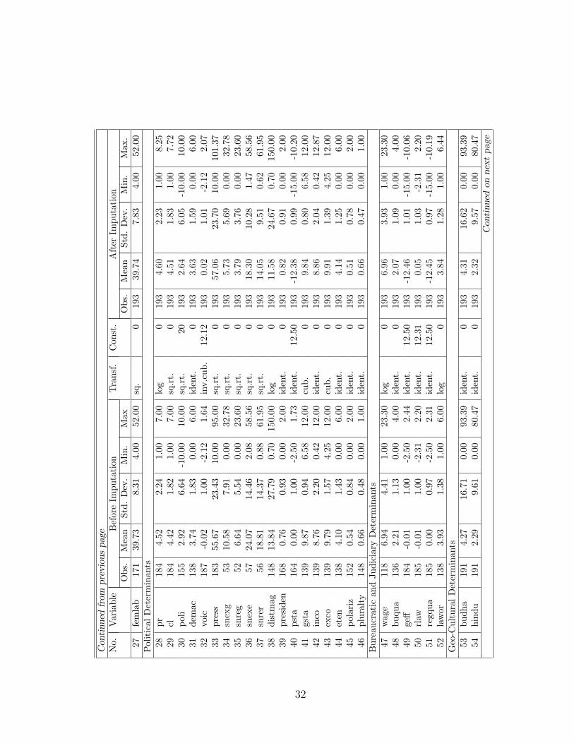
Con
tinued
from
pre
vio
us
page
No.
Var
iabl
eB
efor
eIm
puta
tion
Tra
nsf.
Con
st.
Aft
erIm
puta
tion
Obs
.M
ean
Std.
Dev
.M
in.
Max
Obs
.M
ean
Std.
Dev
.M
in.
Max
.27
fem
lab
171
39.7
38.
314.
0052
.00
sq.
019
339
.74
7.83
4.00
52.0
0Pol
itic
alD
eter
min
ants
28pr
184
4.52
2.24
1.00
7.00
log
019
34.
602.
231.
008.
2529
cl18
44.
421.
821.
007.
00sq
.rt.
019
34.
511.
831.
007.
7230
poli
155
2.92
6.64
-10.
0010
.00
sq.r
t.20
193
2.64
6.05
-10.
0010
.00
31de
mac
138
3.74
1.83
0.00
6.00
iden
t.0
193
3.63
1.59
0.00
6.00
32vo
ic18
7-0
.02
1.00
-2.1
21.
64in
v.cu
b.12
.12
193
0.02
1.01
-2.1
22.
0733
pres
s18
355
.67
23.4
310
.00
95.0
0sq
.rt.
019
357
.06
23.7
010
.00
101.
3734
snex
g53
10.5
87.
910.
0032
.78
sq.r
t.0
193
5.73
5.69
0.00
32.7
835
snre
g52
6.64
5.54
0.00
23.6
0sq
.rt.
019
33.
793.
760.
0023
.60
36sn
exe
5724
.07
14.4
62.
0858
.56
sq.r
t.0
193
18.3
010
.28
1.47
58.5
637
snre
r56
18.8
114
.37
0.88
61.9
5sq
.rt.
019
314
.05
9.51
0.62
61.9
538
dist
mag
148
13.8
427
.79
0.70
150.
00lo
g0
193
11.5
824
.67
0.70
150.
0039
pres
iden
168
0.76
0.93
0.00
2.00
iden
t.0
193
0.82
0.91
0.00
2.00
40ps
ta16
40.
001.
00-2
.50
1.73
iden
t.12
.50
193
-12.
380.
99-1
5.00
-10.
2041
gsta
139
9.87
0.94
6.58
12.0
0cu
b.0
193
9.84
0.80
6.58
12.0
042
inco
139
8.76
2.20
0.42
12.0
0id
ent.
019
38.
862.
040.
4212
.87
43ex
co13
99.
791.
574.
2512
.00
cub.
019
39.
911.
394.
2512
.00
44et
en13
84.
101.
430.
006.
00id
ent.
019
34.
141.
250.
006.
0045
pola
riz
152
0.54
0.84
0.00
2.00
iden
t.0
193
0.51
0.78
0.00
2.00
46pl
ural
ty14
80.
660.
480.
001.
00id
ent.
019
30.
660.
470.
001.
00B
urea
ucra
tic
and
Judi
ciar
yD
eter
min
ants
47w
age
118
6.94
4.41
1.00
23.3
0lo
g0
193
6.96
3.93
1.00
23.3
048
buqu
a13
62.
211.
130.
004.
00id
ent.
019
32.
071.
090.
004.
0049
geff
184
-0.0
11.
00-2
.50
2.44
iden
t.12
.50
193
-12.
461.
01-1
5.00
-10.
0650
rlaw
185
-0.0
11.
00-2
.31
2.20
iden
t.12
.31
193
0.05
1.03
-2.3
12.
2051
regq
ua18
50.
000.
97-2
.50
2.31
iden
t.12
.50
193
-12.
450.
97-1
5.00
-10.
1952
law
or13
83.
931.
381.
006.
00lo
g0
193
3.84
1.28
1.00
6.44
Geo
-Cul
tura
lD
eter
min
ants
53bu
dha
191
4.27
16.7
10.
0093
.39
iden
t.0
193
4.31
16.6
20.
0093
.39
54hi
ndu
191
2.29
9.61
0.00
80.4
7id
ent.
019
32.
329.
570.
0080
.47
Conti
nued
onnex
tpag
e
32

Con
tinued
from
pre
vio
us
pag
eN
o.V
aria
ble
Bef
ore
Impu
tati
onTra
nsf.
Con
st.
Aft
erIm
puta
tion
Obs
.M
ean
Std.
Dev
.M
in.
Max
Obs
.M
ean
Std.
Dev
.M
in.
Max
.55
mus
lim19
125
.60
36.5
40.
0099
.67
iden
t.0
193
25.3
936
.40
0.00
99.6
756
nonr
elig
191
6.20
11.3
60.
0194
.09
log
019
36.
1811
.31
0.01
94.0
957
angl
ic19
12.
727.
680.
0052
.41
iden
t.0
193
2.75
7.65
0.00
52.4
158
cath
ol19
130
.59
32.7
80.
0097
.15
sq.
019
330
.90
32.7
50.
0097
.15
59in
depe
n19
16.
2610
.36
0.01
69.0
0lo
g0
193
6.21
10.3
20.
0169
.00
60m
argi
nal
191
1.30
3.64
0.00
36.6
4id
ent.
019
31.
313.
620.
0036
.64
61or
thod
ox19
15.
8017
.45
0.00
89.7
7id
ent.
019
35.
8117
.36
0.00
89.7
762
prot
est
191
14.9
620
.54
0.00
90.6
6sq
.rt.
019
314
.88
20.4
50.
0090
.66
63et
hnoa
148
0.48
0.27
0.00
0.95
sq.r
t.0
193
0.46
0.25
0.00
0.95
64et
hnob
154
0.33
0.30
0.00
1.00
sq.r
t.0
193
0.31
0.28
0.00
1.00
65en
glis
191
0.33
0.47
0.00
1.00
iden
t.0
193
0.33
0.47
0.00
1.00
66so
cial
191
0.18
0.39
0.00
1.00
iden
t.0
193
0.18
0.39
0.00
1.00
67fr
ench
191
0.43
0.50
0.00
1.00
iden
t.0
193
0.42
0.50
0.00
1.00
68ge
rman
191
0.03
0.17
0.00
1.00
iden
t.0
193
0.03
0.17
0.00
1.00
69sc
andi
191
0.03
0.16
0.00
1.00
iden
t.0
193
0.03
0.16
0.00
1.00
70la
titu
191
0.28
0.19
0.00
0.72
sq.r
t.0
193
0.28
0.19
0.00
0.72
71ar
eakm
193
6900
10.8
019
2154
8.00
25.4
017
1000
00.0
0lo
g0
193
6901
38.9
019
2264
9.00
25.4
017
1000
00.0
0
33

In doing the EM iteration, we use GDP per Capita, population density, and countryarea as the predictors, since in terms of the number of observations these are the mostcomplete variables we have at hand.19 After the imputation, we transform the variablesback to the original scales. Table 7 compares the data before and after the imputation.
Now we have a complete data set. The next step is to generate z-scores from theimputed data that have been transformed back to their original scales. This is tohave a new data set with mean zero and unit variance. We drop seven categoricalvariables in this stage because these variables appear as binary dummy variables; thusthe z-scores are not appropriate to be applied for binary values. They are politicalpolarization, plurality, and five legal origins, namely english, socialism, french, german,and scandinavia.
Having the z-score at hand, we do EFA to uncover the latent structure (called alsodimensions or factors) of our data set and to reduce attribute space from a larger num-ber of variables to a smaller number of factors. Moreover, to have a clearer structureand an easier interpretation of the factors, we rotate the loadings by employing thevarimax method. The varimax searches for an orthogonal rotation (i.e., a linear com-bination) of the original factors such that the variance of the loadings is maximized.Each factor will tend to have either large or small loadings of any particular variable.
In Table 8 we have selected five out of 43 rotated factors that consist of at least twovariables with very high factor loadings (i.e., > 0.710 or < −0.710)20 In Factor 1 thereare 12 variables clustered together with high factor loadings, namely rule of law, judicialindependence and impartial court (area2b of Fraser index), government effectiveness,GDP per capita, political stability, regulatory quality, bureaucratic quality, law andorder, labor market regulation (area5b of Fraser index), international trade (area4b ofFraser index), internal conflict, and secondary school enrolment. Clearly, this factor isdominated by variables reflecting the capacity of government to regulate and enforcelaw. Therefore, we call this factor regulatory capacity.
19Since we have seven binary dummy variables, we follow a simple rule to maintain their originalscale: it takes one if the predicted value is >0.500, and zero otherwise.
20In our case, these benchmark make the pattern of the factors are much clearer. At the same time,they are also reasonable as the squares of these values exceed 0.500, implying that more than 50%proportion of each manifest variable is explained by the factor.
34

Table 8: Selected Rotated Factor Loadings
No Variable Factor 1 Factor 2 Factor 3 Factor 4 Factor 5 ... Factor 43 Uniqueness1 rlaw 0.929 0.108 -0.075 0.033 -0.225 0.116 0.0152 geff 0.893 0.095 -0.091 0.010 -0.214 0.077 0.0513 area2ab 0.892 0.209 -0.091 0.054 -0.160 -0.048 0.0404 gdpcap 0.850 0.152 -0.082 0.129 -0.155 -0.104 0.0555 psta 0.817 -0.007 -0.029 0.115 -0.240 0.011 0.0606 regqua 0.815 0.009 0.018 -0.012 -0.359 0.046 0.0607 buqua 0.809 0.160 -0.127 0.059 -0.292 -0.006 0.1098 lawor 0.776 0.136 -0.152 0.054 -0.009 0.044 0.1359 area5b 0.766 0.031 0.034 0.115 -0.165 -0.047 0.167
10 area4b 0.743 0.110 -0.043 0.169 -0.134 -0.150 0.18011 inco 0.728 -0.018 -0.011 0.104 -0.116 0.079 0.13912 enrols 0.710 0.132 -0.152 0.041 -0.225 -0.023 0.11013 snexe 0.059 0.954 0.002 -0.086 0.005 0.028 0.00814 snrer 0.051 0.949 0.033 -0.027 0.025 0.027 0.01415 snreg 0.323 0.858 -0.046 0.019 -0.076 -0.064 0.01616 snexg 0.392 0.821 -0.082 -0.019 -0.108 -0.054 0.01217 rich20 -0.104 -0.011 0.909 -0.008 -0.007 0.036 0.13118 gini -0.234 -0.079 0.852 -0.032 0.070 -0.001 0.08419 rich10 -0.120 0.041 0.832 -0.066 -0.063 -0.046 0.19720 open 0.126 -0.026 -0.028 0.987 -0.036 0.004 0.00021 mpor 0.065 -0.102 -0.001 0.925 -0.045 -0.014 0.00422 xpor 0.150 0.058 -0.051 0.909 -0.037 0.012 0.00623 pr 0.454 -0.010 0.051 0.033 -0.834 0.014 0.04124 press 0.521 0.013 -0.037 0.046 -0.768 -0.037 0.05825 poli 0.289 0.132 0.063 0.029 -0.768 -0.017 0.14926 cl 0.542 -0.034 0.015 0.036 -0.756 0.054 0.03127 voic 0.601 0.001 -0.031 0.038 -0.749 0.002 0.00928 area3 0.699 0.062 0.020 -0.080 -0.067 -0.289 0.26829 presiden 0.469 -0.029 -0.188 0.079 -0.313 0.019 0.34330 eten 0.429 -0.045 -0.003 -0.039 0.030 -0.036 0.38431 exco 0.400 -0.079 0.012 0.155 -0.305 -0.004 0.38332 latitu 0.376 0.336 -0.299 0.041 -0.135 -0.012 0.22433 demac 0.366 0.155 -0.127 0.046 -0.693 -0.046 0.18634 enrolt 0.309 0.049 -0.089 -0.060 -0.044 -0.018 0.58335 gsta 0.232 0.120 0.096 0.004 0.327 -0.007 0.40336 efherit 0.219 0.013 -0.096 0.016 0.087 -0.009 0.59337 enrolp 0.217 -0.022 0.065 0.100 -0.101 0.011 0.42738 debtcap 0.175 0.238 -0.026 -0.057 -0.098 -0.026 0.43339 popden 0.171 -0.157 -0.039 0.132 0.021 0.000 0.17240 protest 0.170 0.059 0.071 -0.002 -0.238 0.002 -0.002
Continued on next page
35

Continued from previous pageNo Variable Factor 1 Factor 2 Factor 3 Factor 4 Factor 5 . . . Factor 43 Uniqueness41 cathol 0.134 -0.080 0.126 0.107 -0.271 -0.007 -0.00242 anglic 0.128 -0.124 -0.013 -0.001 -0.070 -0.001 -0.00143 nonrelig 0.097 0.209 -0.128 0.011 0.037 -0.001 -0.00244 wage 0.053 -0.346 0.098 0.041 0.040 0.007 0.39045 marginal 0.041 -0.104 0.024 -0.005 -0.091 0.000 0.00546 distmag 0.005 0.110 -0.011 0.211 -0.103 -0.004 0.54647 hindu -0.014 -0.009 -0.051 -0.014 -0.057 -0.001 -0.00148 budha -0.037 -0.038 -0.066 -0.061 0.086 0.003 -0.00249 indepen -0.054 0.044 0.270 0.008 -0.036 0.003 -0.00150 aidcap -0.062 -0.136 -0.031 0.074 -0.141 -0.008 0.42451 govcon -0.069 0.114 -0.043 0.138 0.112 -0.007 0.48052 areakm -0.075 0.580 0.049 0.219 -0.009 0.097 0.22653 area1 -0.083 -0.168 0.212 0.015 0.013 -0.006 0.32854 debtgdp -0.087 -0.159 -0.042 -0.002 0.033 -0.051 0.39355 orthodox -0.095 0.044 -0.135 0.083 -0.081 0.003 -0.00356 xmetal -0.121 0.054 0.122 -0.072 -0.042 -0.025 0.70757 femlab -0.150 0.049 -0.188 0.012 -0.322 -0.017 0.30958 xfuel -0.175 0.221 0.028 0.032 0.234 -0.008 0.49359 muslim -0.194 -0.005 -0.082 -0.104 0.414 0.000 -0.00260 ethnob -0.421 0.046 0.141 -0.003 0.063 -0.052 0.27161 debt -0.433 -0.092 0.050 -0.014 -0.021 0.136 0.38462 ethnoa -0.455 0.142 0.136 -0.054 0.047 0.054 0.23263 illi -0.492 -0.052 0.079 -0.182 0.174 -0.003 0.148
36
Factor 2 includes all proxies of sub national government expenditures and revenues;thus we call this federalism. In Factor 3 we have three variables measuring incomeinequality, namely gini ratio, the richest 10%, and the richest 20%). We call thisfactor inequality. In Factor 4 there are three measures of international trade clusteredtogether, namely export ratio, import ratio, and trade volume; thus we call it trade.Finally, Factor 5 may explain political liberty since it captures five correlated politicalvariables, namely political right, press freedom, polity index, civil librety, and voice.We call this factor political liberty.
Now taking only variables with substantial loadings (thus ignoring the remainingvariables with minor loadings), we generate five new indexes on the basis of the z-scores.These factor-based indexes are computed as follows:
Fi =∑
j
βij
λi
Xj (5)
where F is the index we want to construct, X ’s are the underlying variables (z-score)of the index with high factor loadings, β is the rotated factor loading, and λ is theeigenvalue. This formula is applied for every index we construct.
Graphs 1-5 display the plots of corruption against the five new indexes.21 It isobvious from the Plots that only ’regulatory capacity’ and ’political liberty’ are relatedto corruption. The R2 of the first plot is 0.86 and the fifth’s is 0.44, while the rest arefar below these values. Although suggestive, these results are only based on bivariateregressions. The next section examines whether these newly generated indexes (andthe other non-clustered variables) are robustly correlated with corruption, but first weoutline our methodology.
21Compared to the other four factor loadings, the loadings of variables falling in political liberty areall negative. Hence the interpretation should be reversed: higher scores indicate less political freedom.
37

Plot 1: Plot 2:
Corruption vs Regulatory Capacity
Y = 0.05 - 1.80X
R2 = 0.86
-3.00
-2.00
-1.00
0.00
1.00
2.00
3.00
-1.50 -1.00 -0.50 0.00 0.50 1.00 1.50
Corruption vs Federalism
Y = 0.05 - 0.50X
R2 = 0.10
-3.00
-2.50
-2.00
-1.50
-1.00
-0.50
0.00
0.50
1.00
1.50
2.00
-2.00 -1.00 0.00 1.00 2.00 3.00 4.00
Plot 3: Plot 4:
Corruption vs Inequality
Y = 0.05 + 0.37X
R2 = 0.06
-3.00
-2.50
-2.00
-1.50
-1.00
-0.50
0.00
0.50
1.00
1.50
2.00
-2.00 -1.00 0.00 1.00 2.00 3.00 4.00
Corruption vs Trade
Y =0.05 - 0.19X
R2 = 0.03
-3.00
-2.50
-2.00
-1.50
-1.00
-0.50
0.00
0.50
1.00
1.50
2.00
-2.00 0.00 2.00 4.00 6.00 8.00
Plot 5:
Corruption vs Political Liberty
Y = 0.05 + 0.52X
R2 = 0.44
-3.00
-2.50
-2.00
-1.50
-1.00
-0.50
0.00
0.50
1.00
1.50
2.00
-3.00 -2.00 -1.00 0.00 1.00 2.00 3.00
Scatter Plots 1-5: Corruption vs New Indexes
38

5 Extreme Bounds Analysis
Like in empirical growth models (Temple, 2000), model uncertainty is an importantproblem in empirical models of the causes of corruption. Researchers usually report apreferred model followed by the results of some diagnostic tests. However, the problemis that ”several different models may all seem reasonable given the data, but lead tovery different conclusions about the parameters of interest” (Temple, 2000). In sucha situation, reporting the result of a single preferred model is misleading, since itunderestimates the uncertainty actually present about the parameters. At the sametime, there is no strong theoretical framework to help researchers establishing a properregression model for corruption. This results in a large variety of corruption regressionmodels as well as ways to examine the robustness of variables of interest.
One way to cope with model uncertainty is the extreme bound analysis (EBA).22
The idea behind EBA is to report an upper and lower bound for parameter estimates,that is to examine the sensitivity of parameters to model specification. In this paperwe use the EBA of Levine and Renelt (1992) and Sala-i-Martin’s (1997). We include alarge number of variables that have been claimed to be related to corruption in previousstudies. Our study addresses the question of how much confidence one should have inthe conclusion of previous studies.
The EBA can be exemplified as follows (Leamer, 1983; Levine and Renelt, 1992):
Y = αj + βijI + βmjM + βzjZj + u (6)
where Y is the dependent variable (Kaufmann’s corruption index 2004); I is a vectorof ”standard” explanatory variables (which may be zero); M is the variable of interest;Z is a vector of up-to-three possible additional explanatory variables, which accordingto the literature may be related to the dependent variable; and u is an error term.It should be noted that number of variables in I and Z that can be plugged intothe model is constrained by the degrees of freedom of the regression as well as theissue of multicollinearity. Levine and Renelt (1992) include three variables (the ”fixed-trio”) in I and all possible combinations of up-to-three variables (the ”flex-trio”) in Z.However, due to the lack of theoretical guidance and the wide variety of results reportedin previous studies, we have decided not to include any variable in the I vector.23
The test of extreme bounds for variable M says that if the lower extreme bound forβ —i.e., the lowest value for β minus two standard deviations— is negative, while the
22There is a growing literature starting with Leamer (1983) and Levine and Renelt (1992), followedby a critique by Sala-i-Martin (1997) and Durlauf and Quah (1999). Recently, Doppelhofer et al.(2005) have proposed Bayesian Averaging of Classical Estimates (BACE) approach to check the ro-bustness of different explanatory variables in growth regressions, while Hendry and Krolzig (2004)suggest the General Unrestricted Model (GUM) which basically needs very few regression to test therobustness of a variable of interest.
23Later on, after finding a robust variable(s), we also include this (these) variable(s) in I.
39

upper extreme bound for β —i.e. the highest value for β plus two standard deviations—is positive, the variable M is not robustly related to Y . More formally, the upper andlower bounds are defined as (Levine and Renelt, 1992):
maxmin βmj ± n σβmj
(7)
where n = 2, and σβmjis standard deviation of βmj. The robustness thus has two prop-
erties. First, the coefficients of βmj in the upper and lower bounds must be consistent.Second, they are significant at the conventional level under various conditioning setsof Z. A violation against these properties makes a variable to be regarded as fragile.
Sala-i-Martin (1997), however, rightly argues that the test applied in the Leamer’sas well as the Levine and Renelt’s EBA is too strong for any variable to really pass it.If the distribution of the parameter of interest has some positive and some negativesupports, one is bound to find one regression for which the estimated coefficient changessign if enough regressions are run. He therefore suggests analyzing the entire distrib-ution of the estimates of the parameter of interest. Broadly speaking, if the averaged90% confidence interval of a regression coefficient does not include zero, Sala-i-Martinclassifies the corresponding regressor as a variable that is robust.
In our empirical analysis we will use both versions of the EBA. But, since we agreewith the critique of Sala-i-Martin (1997) on Leamer’s (and Levine and Renelt’s) versionof the EBA, our conclusion will be based on the Sala-i-Martin variant of the EBA. Wenot only report the unweighted parameter estimates of β and fraction of regressionssignificant at 5%, but also the outcomes of the cumulative distribution function (CDF)test. The CDF test is based on the fraction of the cumulative distribution functionlying on each side of zero. Since zero divides CDF into two areas (CDF[0] or 1-CDF[0]),no matter whether it is below or above zero, attention is paid only to the largest of thetwo areas, that is
CDF = max[CDF (0), 1 − CDF (0)] (8)
CDF(0) indicates the larger of the areas under the density function either above orbelow zero, regardless of whether this is CDF(0) or 1-CDF(0). So CDF(0) will alwaysbe a number between 0.5 and 1.0. However, instead of using the 90% criterion, weadvocate a more stringent criterion, i.e., 95% because of the one-sidedness of the test(Sturm and De Haan, 2005).
Some assumptions must be made to calculate the CDF using the integrated likeli-hood (L), the point estimate (βmj), and the standard deviation (σ2
mj). First, if βm isdistributed normally, the weighted mean is obtained by
βm =V∑
j=1
Lmj∑Vi=1 Lzi
βmj
40
and the weighted mean of variance is
σ2m =
V∑j=1
Lmj∑Vi=1 Lzi
σ2mj.
Second, if the distribution of βm is non-normal, the aggregate CDF can be computedusing the individual CDF (Φmj(βmj, σ
2mj)) and the weighted likelihood as before:
Φm =V∑
j=1
Lmj∑Vi=1 Lzi
Φmj(βmj, σ2mj)
After knowing its distribution, a variable is labelled robust if 95% of the density functionfor βm lies to the right or left of zero.
We have 48 variables to be used in the EBA, since 27 variables have been replacedby five new indexes.24 The total number of regressions we run is v!
3!(v−3)!; with 48
variables and no I we have 778,320 total regressions or 16,215 regressions per variablewe test. In Table 9 columns 3-5 show the outcomes of Leamer’s variant of EBA, namelythe lower and upper extreme bounds and the fraction of the regressions in which thevariable is significantly different from zero. Columns 6-12 show the results of Sala-i-Martin’s variant of EBA, namely the estimated coefficients and standard errors aswell as normal and non-normal CDF(0). The variables are ordered on the basis of thenormal CDF(0).
24Now we include the eight categorical variables that were dropped in the factor analysis.
41

Tab
le9:
Extr
eme
Bou
nds
Anal
ysi
s:N
oV
aria
ble
in’I
’
No
Dep
ende
ntLea
mer
Sala
-i-M
arti
nV
aria
ble
Low
erU
pper
Frac
tion
Wei
ghte
dU
nwei
ghte
dN
orm
alN
on-N
orm
alC
DF
Bou
ndB
ound
Sign
f.at
5%B
eta
St.D
ev.
Bet
aSt
.Dev
.C
DF
Wei
ghte
dU
nwgh
t.1
regc
ap-2
.242
-1.4
2610
0.00
0-1
.783
0.06
1-1
.808
0.06
51.
000
1.00
01.
000
2sc
andi
-3.7
860.
488
99.8
33-0
.685
0.07
8-1
.872
0.15
81.
000
1.00
01.
000
3po
pden
-0.0
00+
0.00
099
.093
-0.0
000.
000
-0.0
000.
000
1.00
01.
000
0.99
54
eten
-0.4
480.
121
97.3
730.
072
0.02
0-0
.190
0.05
31.
000
1.00
00.
933
5so
cial
-0.2
743.
210
94.5
730.
232
0.05
80.
588
0.14
51.
000
1.00
00.
994
6no
nrel
ig-0
.055
0.03
112
.081
0.00
60.
002
-0.0
020.
007
1.00
00.
993
0.56
17
illi
-0.0
100.
043
99.7
41-0
.004
0.00
10.
019
0.00
30.
999
0.99
50.
936
8w
age
-0.0
710.
086
18.6
930.
015
0.00
60.
014
0.01
50.
992
0.98
80.
759
9ar
ea3
-0.5
000.
105
94.3
450.
049
0.02
1-0
.308
0.04
10.
991
0.98
50.
939
10la
titu
-4.6
770.
503
93.8
27-0
.452
0.21
5-1
.959
0.37
30.
982
0.91
60.
978
11xf
uel
-0.0
080.
021
74.0
120.
002
0.00
10.
007
0.00
30.
957
0.95
60.
954
12en
rolp
-0.0
200.
015
71.4
830.
003
0.00
1-0
.006
0.00
30.
955
0.95
20.
855
13de
bt-0
.002
0.00
992
.390
-0.0
010.
000
0.00
30.
001
0.95
40.
951
0.93
314
pres
iden
-0.8
250.
029
94.3
57-0
.056
0.03
3-0
.482
0.07
00.
954
0.95
20.
997
15fe
mla
b-0
.041
0.04
811
.964
-0.0
060.
004
0.00
50.
008
0.95
00.
914
0.63
816
ethn
oa-0
.510
2.45
492
.982
-0.1
740.
108
1.21
20.
244
0.94
60.
933
0.94
217
exco
-0.4
170.
091
91.6
440.
030
0.02
1-0
.211
0.04
00.
927
0.92
40.
939
18ai
dcap
-0.0
010.
003
24.2
980.
000
0.00
00.
001
0.00
00.
924
0.91
60.
875
19ar
ea1
-0.1
670.
351
31.8
780.
027
0.02
10.
096
0.05
80.
901
0.86
10.
901
20in
equa
l-0
.222
0.84
880
.401
0.06
00.
047
0.27
10.
094
0.90
10.
867
0.96
721
fren
ch-1
.268
2.92
526
.562
-0.0
640.
056
0.17
60.
130
0.87
40.
836
0.78
822
germ
an-2
.684
1.35
692
.821
-0.1
540.
140
-1.1
590.
285
0.86
30.
855
0.98
023
mar
gina
l-0
.069
0.05
68.
967
0.00
70.
007
0.00
00.
012
0.85
40.
844
0.53
924
polli
b-0
.071
0.72
693
.617
0.03
30.
032
0.44
60.
045
0.84
80.
840
0.99
225
pola
riz
-0.8
980.
087
93.3
70-0
.036
0.03
8-0
.472
0.08
60.
825
0.79
90.
994
26de
btgd
p-0
.012
0.01
132
.865
0.00
10.
001
0.00
30.
002
0.80
50.
781
0.86
727
inde
pen
-0.0
230.
041
9.12
70.
002
0.00
30.
006
0.00
60.
782
0.77
20.
794
Con
tinued
onnex
tpag
e
42

Conti
nued
from
pre
vio
us
pag
eN
oD
epen
dent
Lea
mer
Sala
-i-M
arti
nV
aria
ble
Low
erU
pper
Frac
tion
Wei
ghte
dU
nwei
ghte
dN
orm
alN
on-N
orm
alC
DF
Bou
ndB
ound
Sign
f.at
5%B
eta
St.D
ev.
Bet
aSt
.Dev
.C
DF
Wei
ghte
dU
nwgh
t.28
budh
a-0
.014
0.01
71.
560
-0.0
020.
002
0.00
20.
003
0.78
00.
773
0.64
929
hind
u-0
.025
0.02
37.
832
-0.0
020.
002
-0.0
010.
004
0.74
40.
741
0.55
530
debt
cap
0.00
00.
000
56.2
380.
000
0.00
00.
000
0.00
00.
738
0.71
90.
915
31di
stm
ag-0
.010
0.01
21.
122
0.00
00.
001
-0.0
010.
003
0.73
50.
681
0.59
432
efhe
rit
-0.5
960.
146
71.4
28-0
.021
0.03
6-0
.223
0.09
60.
722
0.71
90.
963
33fe
dera
l-1
.074
0.21
690
.052
-0.0
260.
044
-0.4
010.
100
0.71
90.
685
0.98
834
dem
ac-0
.466
0.16
787
.512
-0.0
110.
020
-0.2
450.
043
0.71
00.
708
0.96
035
trad
e-0
.585
0.23
90.
432
0.01
90.
042
-0.1
300.
116
0.67
70.
679
0.82
236
angl
ic-0
.050
0.02
532
.544
-0.0
010.
003
-0.0
140.
009
0.65
30.
649
0.89
437
gsta
-0.5
210.
157
61.8
130.
010
0.02
9-0
.176
0.07
80.
644
0.63
70.
926
38or
thod
ox-0
.014
0.02
332
.821
0.00
00.
001
0.00
40.
003
0.63
10.
589
0.85
239
cath
ol-0
.015
0.00
948
.930
0.00
00.
001
-0.0
040.
002
0.60
40.
600
0.82
140
prot
est
-0.0
270.
019
73.5
430.
000
0.00
2-0
.010
0.00
40.
580
0.57
50.
950
41go
vcon
-1.3
472.
207
10.5
890.
036
0.18
70.
390
0.38
00.
575
0.57
70.
785
42en
rolt
-0.0
280.
004
92.8
710.
000
0.00
2-0
.012
0.00
40.
564
0.56
30.
967
43ar
eakm
0.00
00.
000
5.90
80.
000
0.00
00.
000
0.00
00.
561
0.56
10.
555
44et
hnob
-0.3
142.
275
93.3
150.
012
0.10
61.
119
0.18
90.
545
0.54
30.
958
45xm
etal
-0.0
140.
032
23.1
210.
000
0.00
30.
008
0.00
60.
538
0.53
10.
870
46pl
ural
ty-0
.234
1.06
284
.823
0.00
40.
062
0.42
10.
132
0.52
30.
521
0.97
047
engl
is-1
.620
2.66
026
.568
0.00
30.
064
-0.1
820.
140
0.51
60.
513
0.81
448
mus
lim-0
.011
0.01
773
.981
0.00
00.
001
0.00
50.
002
0.50
90.
516
0.87
0
43
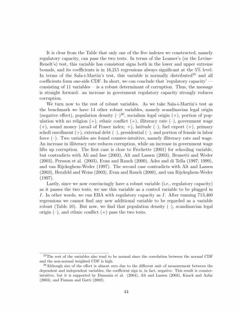
It is clear from the Table that only one of the five indexes we constructed, namelyregulatory capacity, can pass the two tests. In terms of the Leamer’s (or the Levine-Renelt’s) test, this variable has consistent signs both in the lower and upper extremebounds, and its coefficients is in 16,215 regressions always significant at the 5% level.In terms of the Sala-i-Martin’s test, this variable is normally distributed25 and allcoefficients form one-side CDF. In short, we can conclude that ’regulatory capacity’ —consisting of 11 variables— is a robust determinant of corruption. Thus, the messageis straight forward: an increase in government regulatory capacity strongly reducescorruption.
We turn now to the rest of robust variables. As we take Sala-i-Martin’s test asthe benchmark we have 14 other robust variables, namely scandinavian legal origin(negative effect), population density (–)26, socialism legal origin (+), portion of pop-ulation with no religion (+), ethnic conflict (+), illiteracy rate (–), government wage(+), sound money (area3 of Fraser index; +), latitude (–), fuel export (+), primaryscholl enrollment (+), external debt (–), presidential (–), and portion of female in laborforce (–). Two variables are found counter-intuitive, namely illiteracy rate and wage.An increase in illiteracy rate reduces corruption, while an increase in government wagelifts up corruption. The first case is close to Frechette (2001) for schooling variable,but contradicts with Ali and Isse (2003), Alt and Lassen (2003), Brunetti and Weder(2003), Persson et al. (2003), Evan and Rauch (2000), Ades and di Tella (1997; 1999),and van Rijckeghem-Weder (1997). The second case contradicts with Alt and Lassen(2003), Herzfeld and Weiss (2003), Evan and Rauch (2000), and van Rijckeghem-Weder(1997).
Lastly, since we now convincingly have a robust variable (i.e., regulatory capacity)as it passes the two tests, we use this variable as a control variable to be plugged inI. In other words, we run EBA with regulatory capacity as I. After running 713,460regressions we cannot find any new additional variable to be regarded as a variablerobust (Table 10). But now, we find that population density (–), scandinavian legalorigin (–), and ethnic conflict (+) pass the two tests.
25The rest of the variables also tend to be normal since the correlation between the normal CDFand the non-normal weighted CDF is high.
26Although size of the effect is almost zero due to the different unit of measurement between thedependent and independent variables, the coefficient sign is, in fact, negative. This result is counter-intuitive, but it is supported by Damania et al. (2004), Alt and Lassen (2003), Knack and Azfar(2003), and Fisman and Gatti (2002).
44
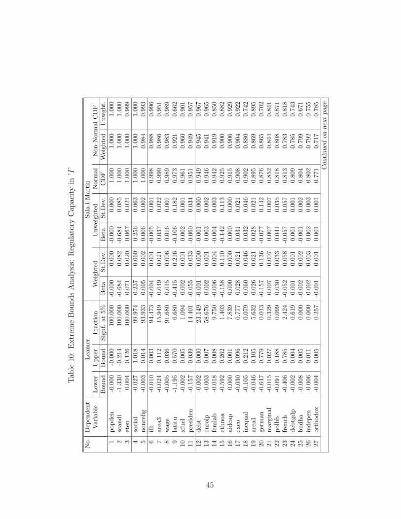
Tab
le10
:E
xtr
eme
Bou
nds
Anal
ysi
s:R
egula
tory
Cap
acity
in’I
’
No
Dep
ende
ntLea
mer
Sala
-i-M
arti
nV
aria
ble
Low
erU
pper
Frac
tion
Wei
ghte
dU
nwei
ghte
dN
orm
alN
on-N
orm
alC
DF
Bou
ndB
ound
Sign
f.at
5%B
eta
St.D
ev.
Bet
aSt
.Dev
.C
DF
Wei
ghte
dU
nwgh
t.1
popd
en-0
.000
-0.0
0010
0.00
0-0
.000
0.00
0-0
.000
0.00
01.
000
1.00
01.
000
2sc
andi
-1.3
30-0
.214
100.
000
-0.6
840.
082
-0.6
840.
085
1.00
01.
000
1.00
03
eten
0.00
40.
126
100.
000
0.07
10.
020
0.06
70.
021
1.00
01.
000
0.99
94
soci
al-0
.027
1.01
899
.974
0.23
70.
060
0.25
60.
063
1.00
01.
000
1.00
05
nonr
elig
-0.0
030.
014
93.9
330.
005
0.00
20.
006
0.00
21.
000
0.98
40.
993
6ill
i-0
.010
0.00
394
.473
-0.0
040.
001
-0.0
050.
001
0.99
80.
988
0.99
67
area
3-0
.024
0.11
215
.949
0.04
90.
021
0.03
70.
022
0.99
00.
986
0.95
18
wag
e-0
.005
0.03
691
.680
0.01
50.
006
0.01
60.
007
0.98
90.
983
0.98
99
lati
tu-1
.195
0.57
06.
680
-0.4
150.
216
-0.1
060.
182
0.97
30.
921
0.66
210
xfue
l-0
.002
0.00
51.
094
0.00
20.
001
0.00
20.
001
0.96
10.
960
0.90
111
pres
iden
-0.1
570.
039
14.4
01-0
.055
0.03
3-0
.060
0.03
40.
951
0.94
90.
957
12de
bt-0
.002
0.00
023
.149
-0.0
010.
000
-0.0
010.
000
0.94
90.
945
0.96
713
enro
lp-0
.003
0.00
758
.676
0.00
20.
001
0.00
30.
002
0.94
60.
941
0.96
514
fem
lab
-0.0
180.
008
9.75
0-0
.006
0.00
4-0
.004
0.00
30.
942
0.91
90.
850
15et
hnoa
-0.5
920.
262
1.40
3-0
.158
0.11
0-0
.142
0.11
30.
925
0.90
00.
882
16ai
dcap
0.00
00.
001
7.83
90.
000
0.00
00.
000
0.00
00.
915
0.90
60.
929
17ex
co-0
.030
0.09
60.
777
0.02
80.
021
0.03
10.
021
0.90
80.
904
0.92
218
ineq
ual
-0.1
050.
212
0.07
90.
060
0.04
60.
032
0.04
60.
902
0.88
00.
742
19ar
ea1
-0.0
460.
105
5.63
20.
026
0.02
10.
028
0.02
10.
895
0.86
90.
895
20ge
rman
-0.6
470.
779
0.01
3-0
.157
0.13
6-0
.077
0.14
20.
876
0.86
50.
702
21m
argi
nal
-0.0
150.
027
0.32
90.
007
0.00
70.
007
0.00
70.
852
0.84
40.
841
22po
llib
-0.0
910.
188
0.09
90.
030
0.03
30.
041
0.03
50.
818
0.80
80.
871
23fr
ench
-0.4
060.
785
2.42
4-0
.052
0.05
8-0
.057
0.05
70.
813
0.78
30.
818
24de
btgd
p-0
.002
0.00
40.
619
0.00
10.
001
0.00
10.
001
0.80
90.
785
0.74
325
budh
a-0
.008
0.00
50.
000
-0.0
020.
002
-0.0
010.
002
0.80
40.
799
0.67
126
inde
pen
-0.0
060.
011
0.00
00.
002
0.00
30.
002
0.00
30.
802
0.79
20.
755
27or
thod
ox-0
.004
0.00
50.
257
-0.0
010.
001
0.00
10.
001
0.77
10.
717
0.78
5C
onti
nued
onnex
tpag
e
45

Conti
nued
from
pre
vio
us
pag
eN
oD
epen
dent
Lea
mer
Sala
-i-M
arti
nV
aria
ble
Low
erU
pper
Frac
tion
Wei
ghte
dU
nwei
ghte
dN
orm
alN
on-N
orm
alC
DF
Bou
ndB
ound
Sign
f.at
5%B
eta
St.D
ev.
Bet
aSt
.Dev
.C
DF
Wei
ghte
dU
nwgh
t.28
debt
cap
0.00
00.
000
9.75
60.
000
0.00
00.
000
0.00
00.
771
0.74
10.
860
29ef
heri
t-0
.120
0.07
40.
000
-0.0
240.
035
-0.0
220.
037
0.75
50.
750
0.72
330
pola
riz
-0.1
580.
101
0.27
7-0
.026
0.03
9-0
.053
0.03
90.
749
0.72
40.
902
31di
stm
ag-0
.002
0.00
30.
033
0.00
00.
001
0.00
10.
001
0.73
60.
701
0.77
432
ethn
ob-0
.328
0.46
20.
000
0.06
80.
109
-0.0
310.
109
0.73
30.
713
0.61
433
prot
est
-0.0
090.
007
6.95
00.
001
0.00
2-0
.003
0.00
20.
703
0.68
40.
891
34de
mac
-0.0
760.
074
0.00
0-0
.010
0.01
9-0
.015
0.02
10.
694
0.69
20.
752
35fe
dera
l-0
.241
0.13
64.
124
-0.0
210.
044
-0.0
550.
046
0.68
50.
660
0.86
436
trad
e-0
.099
0.13
60.
000
0.02
00.
042
0.02
90.
041
0.68
40.
683
0.76
137
hind
u-0
.008
0.00
70.
000
-0.0
010.
002
-0.0
020.
002
0.67
20.
669
0.74
738
engl
is-0
.411
0.80
20.
586
0.02
30.
065
-0.0
090.
064
0.63
90.
592
0.55
139
gsta
-0.0
900.
116
0.00
00.
009
0.02
80.
014
0.03
30.
632
0.62
60.
656
40ca
thol
-0.0
040.
004
0.00
00.
000
0.00
10.
000
0.00
10.
619
0.61
10.
634
41an
glic
-0.0
120.
011
0.00
0-0
.001
0.00
3-0
.001
0.00
30.
617
0.61
40.
589
42xm
etal
-0.0
060.
008
0.00
00.
001
0.00
30.
000
0.00
20.
596
0.58
70.
518
43go
vcon
-0.5
900.
597
0.00
00.
029
0.18
8-0
.006
0.18
70.
561
0.56
20.
512
44m
uslim
-0.0
040.
004
0.02
00.
000
0.00
10.
000
0.00
10.
543
0.53
20.
591
45en
rolt
-0.0
050.
005
0.00
00.
000
0.00
20.
000
0.00
20.
543
0.54
10.
523
46pl
ural
ty-0
.158
0.21
10.
000
0.00
40.
061
0.03
30.
064
0.52
30.
521
0.69
647
area
km0.
000
0.00
00.
079
0.00
00.
000
0.00
00.
000
0.51
80.
516
0.50
3
46
Up to this point we have succesfully generated five simple factor-based indexes in-corporating only variables with high (rotated factor) loadings. Now we turn to anothercomputation technique to generate the indexes. This is to examine whether differentmethod of index (or score) generation result in different impact of the robustness of thevariables. To do this, we first do Confirmatory Factor Analysis (CFA) on the basis ofthe variables that have been rotatedly grouped in the EFA step27, then we generate theindexes. Different from the previous indexes which are also called factor-based scoresor indexes, our indexes are now usually known as factor scores computed on the basisof regression scoring method as follows:
F = X(B′R−1) (9)
where B is the matrix of factor loadings, X is the matrix of the observed variables,and R is the correlation matrix for the X’s.
Using the resulting indexes we run again the two tests of sensitivity analysis asabove. The results are displayed in Tables 11 (without I ) and 12 (with regulatorycapacity as I ). The results are not much different. Regulatory capacity is again foundrobust as it passes the two tests. The rest of variables perform the similar pattern asin the previous. Thus, we can conclude that the different computation technique doesnot result in different outcomes.
27In other words, we use the prior information drawn from the EFA.
47
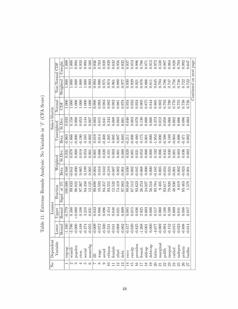
Tab
le11
:E
xtr
eme
Bou
nds
Anal
ysi
s:N
oVar
iable
in’I
’(C
FA
Sco
re)
No
Dep
ende
ntLea
mer
Sala
-i-M
arti
nV
aria
ble
Low
erU
pper
Frac
tion
Wei
ghte
dU
nwei
ghte
dN
orm
alN
on-N
orm
alC
DF
Bou
ndB
ound
Sign
f.at
5%B
eta
St.D
ev.
Bet
aSt
.Dev
.C
DF
Wei
ghte
dU
nwgh
t.1
regc
ap-1
.160
-0.7
7910
0.00
0-0
.946
0.03
1-0
.963
0.03
31.
000
1.00
01.
000
2sc
andi
-3.7
860.
488
99.8
33-0
.641
0.07
8-1
.866
0.15
81.
000
1.00
01.
000
3po
pden
-0.0
00+
0.00
098
.822
-0.0
000.
000
-0.0
000.
000
1.00
01.
000
0.99
44
eten
-0.4
480.
108
97.3
670.
065
0.01
8-0
.190
0.05
31.
000
1.00
00.
933
5so
cial
-0.2
743.
210
94.4
500.
199
0.05
30.
585
0.14
41.
000
1.00
00.
994
6no
nrel
ig-0
.055
0.03
112
.125
0.00
50.
001
-0.0
020.
007
1.00
00.
993
0.56
07
illi
-0.0
090.
043
99.6
98-0
.004
0.00
10.
019
0.00
30.
998
0.99
40.
936
8w
age
-0.0
720.
086
19.5
930.
016
0.00
60.
014
0.01
50.
993
0.99
00.
763
9ar
ea3
-0.5
000.
096
94.3
570.
042
0.02
0-0
.308
0.04
10.
983
0.97
50.
939
10et
hnoa
-0.5
212.
454
93.5
55-0
.210
0.10
11.
205
0.24
30.
982
0.97
40.
939
11fe
mla
b-0
.041
0.04
812
.532
-0.0
070.
003
0.00
50.
008
0.98
20.
961
0.63
212
xfue
l-0
.008
0.02
174
.419
0.00
20.
001
0.00
70.
003
0.98
10.
980
0.95
613
debt
-0.0
020.
009
97.0
83-0
.001
0.00
00.
003
0.00
10.
978
0.97
70.
932
14ex
co-0
.417
0.08
589
.948
0.03
00.
020
-0.2
110.
040
0.93
40.
930
0.93
715
enro
lp-0
.020
0.01
567
.512
0.00
20.
001
-0.0
060.
003
0.93
20.
929
0.85
316
pres
iden
-0.8
250.
036
93.6
23-0
.045
0.03
1-0
.480
0.07
00.
924
0.92
10.
996
17fr
ench
-1.2
682.
925
26.2
53-0
.068
0.05
20.
175
0.13
00.
905
0.87
60.
786
18ai
dcap
-0.0
010.
003
24.0
270.
000
0.00
00.
001
0.00
00.
875
0.86
60.
871
19de
btca
p0.
000
0.00
056
.516
0.00
00.
000
0.00
00.
000
0.84
40.
811
0.91
220
lati
tu-4
.677
0.51
793
.784
-0.1
650.
192
-1.9
530.
373
0.80
50.
645
0.97
221
mar
gina
l-0
.069
0.06
09.
405
0.00
50.
006
0.00
00.
012
0.80
20.
794
0.53
822
polli
b-0
.984
0.10
893
.617
-0.0
340.
042
-0.5
980.
058
0.79
30.
786
0.98
723
ineq
ual
-0.1
520.
599
79.9
200.
024
0.03
00.
189
0.06
60.
790
0.74
70.
964
24ca
thol
-0.0
150.
009
48.9
30-0
.001
0.00
1-0
.004
0.00
20.
770
0.75
60.
828
25in
depe
n-0
.023
0.04
18.
819
0.00
20.
003
0.00
60.
006
0.75
50.
748
0.79
426
pola
riz
-0.8
980.
088
93.4
63-0
.023
0.03
6-0
.471
0.08
60.
738
0.72
20.
992
27bu
dha
-0.0
140.
017
1.57
9-0
.001
0.00
20.
002
0.00
30.
726
0.72
20.
647
Con
tinued
onnex
tpag
e
48

Conti
nued
from
pre
vio
us
pag
eN
oD
epen
dent
Lea
mer
Sala
-i-M
arti
nV
aria
ble
Low
erU
pper
Frac
tion
Wei
ghte
dU
nwei
ghte
dN
orm
alN
on-N
orm
alC
DF
Bou
ndB
ound
Sign
f.at
5%B
eta
St.D
ev.
Bet
aSt
.Dev
.C
DF
Wei
ghte
dU
nwgh
t.28
angl
ic-0
.050
0.02
532
.495
-0.0
020.
003
-0.0
140.
009
0.71
60.
711
0.89
329
dem
ac-0
.466
0.16
887
.512
-0.0
110.
019
-0.2
450.
042
0.71
40.
712
0.96
030
hind
u-0
.025
0.02
37.
789
-0.0
010.
002
-0.0
010.
004
0.70
90.
706
0.55
331
govc
on-1
.347
2.22
310
.688
0.09
40.
183
0.39
80.
381
0.69
70.
693
0.79
832
area
1-0
.167
0.35
131
.853
0.01
00.
019
0.09
60.
058
0.69
60.
659
0.89
533
germ
an-2
.684
1.35
692
.908
-0.0
700.
137
-1.1
530.
285
0.69
50.
692
0.96
734
efhe
rit
-0.5
960.
146
71.4
22-0
.016
0.03
3-0
.222
0.09
60.
686
0.68
20.
962
35di
stm
ag-0
.010
0.01
21.
122
0.00
00.
001
-0.0
010.
003
0.66
60.
632
0.60
236
trad
e-0
.524
0.20
91.
233
0.01
10.
033
-0.1
230.
103
0.62
90.
630
0.83
837
debt
gdp
-0.0
120.
011
33.0
680.
000
0.00
10.
003
0.00
20.
620
0.60
10.
858
38gs
ta-0
.521
0.15
761
.801
0.00
80.
027
-0.1
760.
078
0.61
30.
607
0.92
639
orth
odox
-0.0
140.
023
32.7
470.
000
0.00
10.
004
0.00
30.
600
0.58
50.
853
40pr
otes
t-0
.027
0.02
173
.241
0.00
00.
002
-0.0
100.
004
0.59
30.
583
0.94
141
engl
is-1
.620
2.66
026
.778
-0.0
130.
059
-0.1
810.
140
0.58
80.
582
0.80
842
ethn
ob-0
.312
2.27
593
.315
-0.0
180.
100
1.11
40.
189
0.57
30.
571
0.95
543
mus
lim-0
.011
0.01
775
.153
0.00
00.
001
0.00
50.
002
0.56
80.
554
0.87
544
plur
alty
-0.2
331.
062
84.7
240.
008
0.05
90.
420
0.13
20.
556
0.55
40.
971
45ar
eakm
0.00
00.
000
6.13
60.
000
0.00
00.
000
0.00
00.
552
0.53
90.
554
46xm
etal
-0.0
140.
032
21.7
450.
000
0.00
20.
008
0.00
60.
544
0.54
80.
865
47en
rolt
-0.0
280.
004
92.8
580.
000
0.00
2-0
.012
0.00
40.
526
0.52
60.
962
48fe
dera
l-0
.726
0.13
490
.953
-0.0
010.
029
-0.2
770.
066
0.51
50.
507
0.98
4
49

Tab
le12
:E
xtr
eme
Bou
nds
Anal
ysi
s:R
egula
tory
Cap
acity
in’I
’(C
FA
Sco
re)
No
Dep
ende
ntLea
mer
Sala
-i-M
arti
nV
aria
ble
Low
erU
pper
Frac
tion
Wei
ghte
dU
nwei
ghte
dN
orm
alN
on-N
orm
alC
DF
Bou
ndB
ound
Sign
f.at
5%B
eta
St.D
ev.
Bet
aSt
.Dev
.C
DF
Wei
ghte
dU
nwgh
t.1
popd
en-0
.000
-0.0
0010
0.00
0-0
.000
0.00
0-0
.000
0.00
01.
000
1.00
01.
000
2sc
andi
-1.2
94-0
.191
100.
000
-0.6
430.
082
-0.6
380.
084
1.00
01.
000
1.00
03
soci
al-0
.031
0.92
599
.868
0.20
10.
054
0.21
70.
058
1.00
01.
000
0.99
94
eten
-0.0
020.
113
99.9
930.
064
0.01
80.
058
0.01
91.
000
0.99
90.
998
5no
nrel
ig-0
.003
0.01
293
.630
0.00
50.
001
0.00
50.
002
0.99
90.
986
0.99
26
illi
-0.0
090.
003
93.0
76-0
.003
0.00
1-0
.004
0.00
10.
996
0.98
70.
994
7w
age
-0.0
030.
036
98.2
150.
015
0.00
60.
017
0.00
60.
992
0.98
70.
993
8ar
ea3
-0.0
200.
101
15.9
290.
043
0.02
00.
035
0.02
00.
986
0.97
90.
954
9xf
uel
-0.0
020.
005
9.80
90.
002
0.00
10.
002
0.00
10.
983
0.98
10.
941
10fe
mla
b-0
.018
0.00
626
.166
-0.0
060.
003
-0.0
050.
003
0.97
70.
960
0.94
711
debt
-0.0
020.
000
86.0
47-0
.001
0.00
0-0
.001
0.00
00.
977
0.97
50.
983
12et
hnoa
-0.5
850.
191
13.8
01-0
.197
0.10
2-0
.174
0.10
60.
974
0.96
10.
941
13en
rolp
-0.0
030.
007
5.85
00.
002
0.00
10.
003
0.00
20.
921
0.91
70.
945
14pr
esid
en-0
.137
0.04
50.
560
-0.0
440.
031
-0.0
480.
032
0.92
10.
916
0.92
915
exco
-0.0
280.
090
0.74
40.
028
0.02
00.
030
0.02
00.
920
0.91
40.
928
16fr
ench
-0.3
660.
721
1.54
2-0
.064
0.05
3-0
.053
0.05
40.
886
0.84
90.
818
17de
btca
p0.
000
0.00
016
.094
0.00
00.
000
0.00
00.
000
0.87
00.
826
0.91
218
aidc
ap0.
000
0.00
10.
415
0.00
00.
000
0.00
00.
000
0.86
70.
854
0.89
519
lati
tu-1
.050
0.57
84.
895
-0.1
880.
197
-0.0
540.
174
0.83
10.
706
0.58
020
ineq
ual
-0.0
760.
135
0.00
00.
026
0.03
00.
016
0.03
10.
806
0.77
00.
690
21m
argi
nal
-0.0
140.
024
0.00
00.
005
0.00
60.
006
0.00
60.
801
0.79
20.
818
22ca
thol
-0.0
040.
004
0.00
0-0
.001
0.00
10.
000
0.00
10.
778
0.75
90.
512
23po
llib
-0.2
120.
134
0.00
0-0
.031
0.04
2-0
.037
0.04
50.
773
0.76
50.
789
24in
depe
n-0
.006
0.01
10.
000
0.00
20.
003
0.00
20.
003
0.77
20.
763
0.76
025
budh
a-0
.007
0.00
50.
000
-0.0
010.
002
-0.0
010.
002
0.74
60.
741
0.66
126
area
1-0
.054
0.08
80.
283
0.01
10.
019
0.01
70.
020
0.72
40.
695
0.79
227
dem
ac-0
.074
0.06
20.
000
-0.0
100.
018
-0.0
140.
020
0.71
30.
710
0.75
6C
onti
nued
onnex
tpag
e
50
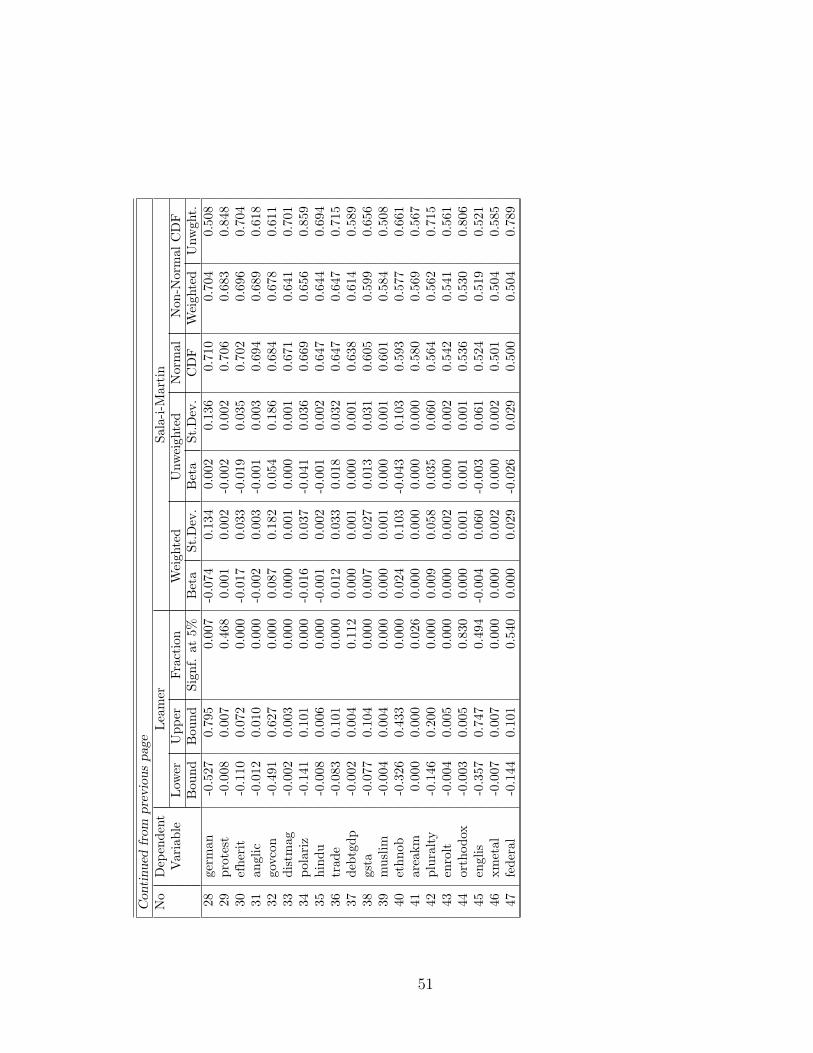
Conti
nued
from
pre
vio
us
pag
eN
oD
epen
dent
Lea
mer
Sala
-i-M
arti
nV
aria
ble
Low
erU
pper
Frac
tion
Wei
ghte
dU
nwei
ghte
dN
orm
alN
on-N
orm
alC
DF
Bou
ndB
ound
Sign
f.at
5%B
eta
St.D
ev.
Bet
aSt
.Dev
.C
DF
Wei
ghte
dU
nwgh
t.28
germ
an-0
.527
0.79
50.
007
-0.0
740.
134
0.00
20.
136
0.71
00.
704
0.50
829
prot
est
-0.0
080.
007
0.46
80.
001
0.00
2-0
.002
0.00
20.
706
0.68
30.
848
30ef
heri
t-0
.110
0.07
20.
000
-0.0
170.
033
-0.0
190.
035
0.70
20.
696
0.70
431
angl
ic-0
.012
0.01
00.
000
-0.0
020.
003
-0.0
010.
003
0.69
40.
689
0.61
832
govc
on-0
.491
0.62
70.
000
0.08
70.
182
0.05
40.
186
0.68
40.
678
0.61
133
dist
mag
-0.0
020.
003
0.00
00.
000
0.00
10.
000
0.00
10.
671
0.64
10.
701
34po
lari
z-0
.141
0.10
10.
000
-0.0
160.
037
-0.0
410.
036
0.66
90.
656
0.85
935
hind
u-0
.008
0.00
60.
000
-0.0
010.
002
-0.0
010.
002
0.64
70.
644
0.69
436
trad
e-0
.083
0.10
10.
000
0.01
20.
033
0.01
80.
032
0.64
70.
647
0.71
537
debt
gdp
-0.0
020.
004
0.11
20.
000
0.00
10.
000
0.00
10.
638
0.61
40.
589
38gs
ta-0
.077
0.10
40.
000
0.00
70.
027
0.01
30.
031
0.60
50.
599
0.65
639
mus
lim-0
.004
0.00
40.
000
0.00
00.
001
0.00
00.
001
0.60
10.
584
0.50
840
ethn
ob-0
.326
0.43
30.
000
0.02
40.
103
-0.0
430.
103
0.59
30.
577
0.66
141
area
km0.
000
0.00
00.
026
0.00
00.
000
0.00
00.
000
0.58
00.
569
0.56
742
plur
alty
-0.1
460.
200
0.00
00.
009
0.05
80.
035
0.06
00.
564
0.56
20.
715
43en
rolt
-0.0
040.
005
0.00
00.
000
0.00
20.
000
0.00
20.
542
0.54
10.
561
44or
thod
ox-0
.003
0.00
50.
830
0.00
00.
001
0.00
10.
001
0.53
60.
530
0.80
645
engl
is-0
.357
0.74
70.
494
-0.0
040.
060
-0.0
030.
061
0.52
40.
519
0.52
146
xmet
al-0
.007
0.00
70.
000
0.00
00.
002
0.00
00.
002
0.50
10.
504
0.58
547
fede
ral
-0.1
440.
101
0.54
00.
000
0.02
9-0
.026
0.02
90.
500
0.50
40.
789
51
6 Conclusion
In this paper we survey the literature on the causes of corruption. The literaturesuggests a long list of variables claimed as statistically significant determinants. Wecollect as many as variables as possible and examine whether suhc claims are alwaysconsistent under various regression specification. We, however, face two problems.First, since the variables are drawn from different sources, these sources do not havethe same set of observations. Thus, we have a missing data problem. Second, as wework with a huge number of variables, inter-dependencies among the determinantsresult in a multicollinearity problem once we run corruption regression.
To cope with the first problem, we do an imputation technique called ’Expectation-Maximization’. Through this techniques we generate a complete set of data consistingof 193 observations and 70 variables. To solve the second problem, we do ExploratoryFactor Analysis in which we reduce the dimension of data. Through this technique, 27variables can be reduced into five new variables, namely ’regulatory capacity’, ’feder-alism’, ’inequality’, ’trade’, and ’political liberty’. For these new variables we generatetwo types of index, namely factor-based score and factor score.
To examine whether these new variables and the other non-clusterred variables arerobust in explaining variation in corruption, we employ two tests of Extreme BoundsAnalysis. Using these two tests, we find that one of our new indexes, namely ’regulatorycapacity’, is the most robust variables. But, using the Sala-i-Martin’s test, we find thatabout 11-14 variables can pass the test. We also find that different index generationstill creates the similar result. In short, we convincingly conclude that ’regulatorycapacity’ is the most robust determinant of corruption. The other robust determinantsare population density (–), scandinavian legal origin (–), ethnic tension (+), socialismlegal origin (+), portion of population with no religion (+), ethnic conflict (+), illiteracyrate (–), government wage (+), sound money (area3 of Fraser index; +), latitude (–),fuel export (+), primary scholl enrollment (+), external debt (–), presidential (–), andportion of female in labor force (–).
52
References
[1] Abed, George T. and Hamid R. Davoodi. 2000. ”Corruption, Structural Reforms,and Economic Performance in the Transition Economies”. IMF Working PaperWP/00/132.
[2] Ades, A. and Di Tella, R. 1997. ”The new economics of corruption: a survey andsome new results”. Political Studies XLV: 496-515.
[3] Ades, A. and Di Tella, R. 1999. ”Rents, Competition, and Corruption”. AmericanEconomic Review 89(4): 982-92.
[4] Ali, M. Abdiweli and Hodan Said Isse. 2003. ”Determinants of Economic Cor-ruption: A Cross-Country Comparison”. Cato Journal 22(3): 449-466.
[5] Alt, James E. and David Dreyer Lassen. 2003. ”The Political Economy of Cor-ruption in American States”. Journal of Theoretical Politics 15(3): 341-365.
[6] Amundsen, Inge. 1999. ”Political Corruption: An Introduction to the Issues”.Chr. Michelsen Institute Development Studies and Human Rights Working Paper7.
[7] Andvig, Jens Chr. 1991. ”The Economics of Corruption: A Survey”. Studi Eco-nomici 43(1): 57-94.
[8] —————. 2005. ”A House of Straw, Sticks or Bricks? Some Notes on Cor-ruption Empirics”. Paper presented at the Fourth Global Forum on FightingCorruption and Safeguarding Integrity.
[9] Andvig, Jens Chr., Odd-Helge Fjeldstad, Inge Amundsen, Tone Sissener, andTina Soreide. 2000. ”Research on Corruption: A Policy Oriented Survey”. Chr.Michelsen Institute and Norwegian Institute of International Affairs.
[10] Bonaglia, Federico, Jorge Braga de Macedo, and Maurizio Bussolo. 2001. ”HowGlobalization Improves Governance”. Discussion Paper No. 2992. Paris, France:Centre for Economic Policy Research, Organisation for Economic Co-operationand Development.
[11] Bowles, Roger. 2000. Corruption. In Boudewijn Bouckaert and Gerrit de Geest(eds.). Encyclopedia of Law and Economics: The Economics of Crime and Liti-gation, Vol. V. Edward Elgar, Cheltenham, UK.
[12] Braun, Miguel and Rafael Di Tella. 2004. ”Inflation, Inflation Variability, andCorruption”. Economics and Politics 16: 77-100.
53

[13] Broadman, Harry G. and Francesca Recanatini. 2000. ”Seed of Corruption: DoMarket Institutions Matter?”. The World Bank Policy Research Working PaperNo. 2368.
[14] —————. 2002. ”Corruption and Policy: Back to the Roots”. Policy Reform5: 37-49
[15] Brown, David S., Michael Touchton, and Andrew B. Whitford. 2005. ”Politi-cal Polarizationas a Constraint on Government: Evidence from Corruption” onSSRN http://ssrn.com/abstract=782845.
[16] Brunetti, Aymo and Beatrice Weder. 2003. ”A Free Press is Bad News for Cor-ruption”. Journal of Public Economics 87:1801-1824.
[17] Caiden, G. E. and Caiden, N.J. 1977. ”Administrative Corruption”. Public Ad-ministration Review 37(3): 301-309.
[18] Chang, Eric CC and Golden, Miriam A. 2004. ”Electoral Systems, District Mag-nitude and Corruption”. Paper presented at the 2003 annual meeting of theAmerican Political Science Association, August 28-31, 2003
[19] Damania, Richard, Per Fredriksson, and Muthukumara Mani, 2004. ”The Persis-tence of Corruption and Regulatory Compliance Failures: Theory and Evidence”.Public Choice 121: 363-390.
[20] Dempster, A. P., N. M. Laird, and D. B. Rubin. 1977. ”Maximum Likelihoodfrom Incomplete Data via the EM Algorithm. Journal of the Royal StatisticalSociety. Series B (Methodological) 45: 289-309.
[21] Doppelhofer, G., R.I. Miller and X. Sala-i-Martin (2000), ”Determinants of Long-term Growth: A Bayesian Averaging of Classical estimates (BACE) Approach”,NBER Working Paper No. 7750.
[22] Durlauf, S.N. and D.T. Quah. 1999. ”The New Empirics of Economic Growth,”in Handbook of Macroeconomics Vol. 1, John B. Taylor and M. Woodford (eds),North Holland, Amsterdam.
[23] Fisman, Raymond J. and Roberta Gatti. 2002. ”Decentralization and Corruption:Evidence across Countries”. Journal of Public Economics 83: 325-345.
[24] Frechette, Guillaume R. 2001. ”A Panel Data Analysis of the Time-Varying De-terminants of Corruption”. Paper presented at the EPCS 2001.
54
[25] Galtung, Fredrick. 2005 (forthcoming). ”Measuring the Immeasurable: Bound-aries and Functions of (Macro) Corruption Indices”. In Fredrick Galtung andCharles Sampford (eds.). Measuring Corruption. Ashgate, UK.
[26] Gatti, R. (1999), ”Corruption and Trade Tariffs, or a Case for Uniform Tariffs”,World Bank Policy Research Working Paper No. 2216.
[27] Glynn, Patrick, Stephen J. Kobrin, and Moises Naim. 1997. The Globalization ofCorruption. In Kimberly Ann Elliott (ed.). Corruption and the Global Economy.Institute for International Economics.
[28] Golden, Miriam A. and Lucio Picci. 2005. ”Proposal for a New Measure of Cor-ruption: Illustrated with Italian Data”. Economics and Politics 17(1): 37-75.
[29] Goldsmith, Arthur A. . 1999. ”Slapping the Grasping Hand: Correlates of Po-litical Corruption in Emerging Market”. American Journal of Economics andSociology 58(4): 865-883.
[30] Gottfredson, Michael, and Travis Hirshi. 1990. A General Theory of Crime. Stan-ford CA: Stanford Univ. Press.
[31] Gould, David J. 1991. ”Administrative Corruption: Incidence, Causes and Re-medial Strategies”. In A. Farazmand (ed.). Handbook of Comparative and Devel-opment Public Administration. Marcel Dekker Inc., New York.
[32] Graeff, P. and Mehlkop, G. 2003. ”The Impacts of Economic Freedom on Cor-ruption: Different Patterns for Rich and Poor Countries”, European Journal ofPolitical Economy 19: 605-620.
[33] Gupta, Sanjeev, Hamid Davoodi, and Rosa Alonso-Terme. 1998 ”Does Corrup-tion Affect Income Inequality and Poverty”. IMF Working Paper 98/76.
[34] Gurgur, Tugrul and Anwar Shah. 2005. ”Localization and Corruption: Panaceaor Pandora’s Box”. World Bank Policy Research Working Paper 3486.
[35] Hall, Robert E. and Jones, Charles I. 1999. ”Why do Some Countries Produce somuch more Output per Worker than Others”. Quarterly Journal of Economics114: 83-116.
[36] Herzfeld, Thomas and Christoph Weiss. 2003. ”Corruption and Legal (In)-Effectiveness: An Empirical Investigation”. European Journal of Political Econ-omy 19: 621-632.
[37] Henderson, J. Vernon and Ari Kuncoro. 2004. ”Corruption in Indonesia”. NBERWorking Paper No. 10674.
55

[38] Hendry, David F. and Hans-Martin Krolzig. 2004. ”We Ran One Regression”.Department of Economics, Oxford University.
[39] Jain, Arvind K. 2001. ”Corruption: A Review”. Journal of Economic Surveys15(1): 71-121.
[40] Jayawickrama, N. 2001. ”Transparency International Combating Corruptionthrough Institutional Reform”. In Annette Y. Lee-Chai and John A. Barg (eds.).The Use and Abuse of Power: Multiple Perspectives on the Causes of Corruption.Psychology Press Philadelphia, Florence, and Sussex.
[41] Johnston, Michael. 2001. ”Measuring Corruption: Number versus Knowledgeversus Understanding”. In Arvind K. Jain (ed.). The Political Economy of Cor-ruption. Routledge, London and New York.
[42] Kaufmann, Daniel and Aart Kraay. 2002a. ”Governance Indicators, Aid Alloca-tion and the Millennium Challenge”. World Bank mimeo.
[43] —————. 2002b. ”Growth Without Governance”. World Bank Policy ResearchWorking Paper No. 2928
[44] Kaufmann, Daniel and Aart Kraay, and Massimo Mastruzzi. 1999. ”GovernanceMatters”. World Bank Policy Research Working Paper 2196.
[45] —————. 2000. ”Governance Matters: From Measurement to Action”. Financeand Development 37(2): 10-13.
[46] —————. 2003. ”Governance Matters III: Governance Indicators for 1996-2002”. World Bank mimeo.
[47] —————. 2005. ”Governance Matters IV: Governance Indicators for 1996-2004”. World Bank mimeo.
[48] Kaufmann, Daniel and Aart Kraay, and Pablo Zoido-Lobatn, P. 1999a. ”Ag-gregating Governance Indicators”. World Bank Policy Research Working Paper2195.
[49] —————. 1999b. ”Governance Matters”. World Bank Policy Research WorkingPaper 2195.
[50] Knack, Stephen and Omar Azfar. 2003. ”Trade Intensity, Country Size and Cor-ruption”. Economics of Governance 4: 1-18.
[51] Kuncoro, Ari. 2004. ”Bribery in Indonesia: Some Evidence from Micro-LevelData”. Bulletin of Indonesian Economic Studies 40(3): 329-354.
56
[52] Kunicova, Jana and Susan Rose-Ackerman. 2005. ”Electoral Rules and Consti-tutional Structures as Constraints on Corruption”, British Journal of PoliticalScience 35 (4): 573-606.
[53] Laffont, Jean J. and Tchetche N’Guessan. 1999. ”Competition and Corruptionin an Agency Relationship”. Journal of Development Economics 60: 271-95.
[54] La Porta, R., Lopez-de-Silanes, F., Shleifer, A., Vishny, R.W. 1998. ”The Qualityof Government”, Journal of Law, Economics, and Organization 15: 222-79.
[55] Lambsdorff, Johann Graf. 1998. ”Transparency International (TI) 1998 Corrup-tion Perception Index, Framework Document”. Transparency International andUniversity of Passau.
[56] ————–. 2000. ”Background Paper to the 2000 Corruption Perceptions Index:Framework Document”. Transparency International and Gottingen University.
[57] ————–. 2001a. ”Background Paper to the 2001 Corruption Perceptions Index:Framework Document”. Transparency International and Gottingen University.
[58] ————–. 2001b. ”How Corruption in Government Affects Public Welfare: AReview of Theory”. Mimeo, Georg-August-University of Gottingen.
[59] ————–. 2002. ”Background Paper to the 2002 Corruption Perceptions Index:Framework Document”. Transparency International and Gottingen University.
[60] ————–. 2003. ”Background Paper to the 2003 Corruption Perceptions Index:Framework Document”. Transparency International and University of Passau.
[61] ————–. 2004a. ”Background Paper to the 2004 Corruption Perceptions Index:Framework Document”. Transparency International and University of Passau.
[62] ————–. 2004b. ”Corruption Perceptions Index 2004”. In Diana Rodriguez,Gerard Waite, and Toby Wolfe (eds.). Global Corruption Report 2005. Trans-parency International-Pluto Press, London.
[63] Leamer, Edward E. 1985. ”Sensitivity Analysis Would Help”, American Eco-nomic Review 75, 308-313.
[64] Lederman, Daniel, Norman V. Loayza, and Rodrigo R. Soares. 2005. ”Account-ability and Corruption: Political Institutions Matter”. Economics and Politics17: 1-35.
[65] Leite, Carlos A. and Jens Weidmann. 1999. ”Does Mother Nature Corrupt?: Nat-ural Resources, Corruption, and Cconomic Growth”. Working paper WP/99/85,International Monetary Fund, Washington, DC.
57

[66] Levine, Ross and David Renelt. 1992. ”A Sensitivity Analysis of Cross-CountryGrowth Regressions.” American Economic Review 82(4): 942-963.
[67] Manzetti, Luigi and Charles Blake. 1996. ”Market Reforms and Corruption inLatin America.” Review of International Political Economy 3: 671-682.
[68] Mauro, Paulo. 1995. ”Corruption and growth.” Quarterly Journal of Economics110(3): 681-712.
[69] Murray-Rust, D. Hammond, and Edward J. Vander Velde. 1994. ”Changes in Hy-draulic Performance and Comparative Costs of Lining and Desilting of SecondaryCanals in Punjab, Pakistan”. Irrigation and Drainage Systems 8(3): 137-158.
[70] Nye, Joseph S. 1967. ”Corruption and Political Development: A Cost-BenefitAnalysis”. The American Political Science Review 61(2): 417-427.
[71] Wehmeier, S (ed.). 2000. Oxford Advanced Learner’s Dictionary of Current Eng-lish. Oxford: Oxford University Press.
[72] Paldam, Martin. 2001. ”Corruption and Religion: Adding to the EconomicModel”. Kyklos 54: 383-414
[73] Paldam, Martin. 2002. ”The Cross-Country Pattern of Corruption: Economics,Culture and the Seesaw Dynamics”. European Journal of Political Economy 18:215-240.
[74] Park, Hoon. 2003. ”Determinants of Corruption: A Cross-National Analysis”The Multinational Business Review 11(2): 29-48.
[75] Paternoster, Raymond and Sally Simpson. 1996. ”Sanction Threats and Appealsto Morality: Testing a Rational Choice Model of Corporate Crime”. Law andSociety Review 30(3): 549583.
[76] Persson, Torsten and Guido Tabellini. 2003. The Economic Effects of Constitu-tions. Cambridge, Mass.: MIT Press.
[77] Persson, Torsten, Guido Tabellini, and Francesco Trebbi. 2003. ”Electoral Rulesand Corruption”. Journal of the European Economic Association 1(4): 958-989.
[78] Rauch, James and Peter Evans. 2000. ”Bureaucratic Structure and BureaucraticPerformance in Less Developed Countries”. Journal of Public Economics 75: 49-71.
[79] Ruud, P. A. 1991. Extentions of Estimation Methods using the EM Algorithm.Journal of Econometrics 49: 305-341.
58
[80] Sala-i-Martin, Xavier. 1997a. ”I Just Ran Four Millions Regressions.” Mimeo,Columbia University.
[81] —————. 1997b. ”I Just Ran Two Millions Regressions.” American EconomicReview, 87(2): 178-183.
[82] Scott, James C. 1972. Comparative Political Corruption. Englewood Cliffs, NJ:Prentice-Hall.
[83] Shleifer, Andrei and Robert W. Vishny. 1993. ”Corruption”. Quarterly Journalof Economics 108(3): 599-617.
[84] Sik, Endre. 2002. ”The Bad, the Worse and the Worst: Guestimating the Levelof Corruption”. In Kotkin, Stephen and Andras Sajo. (eds.) Political Corruptionin Transition: A Skeptic’s Handbook. Budapest; New York: Central EuropeanUniversity Press.
[85] Soreide, Tina. 2003. ”Estimating Corruption: Comments on Available Data”.Chr. Michelsen Institute. Mimeo.
[86] Spearman, Charles. 1904. ”General Intelligence, Objectively Determined andMeasured. American Journal of Psychology 15: 201-293.
[87] Sturm, Jan-Egbert and Jakob de Haan. Forthcoming. ”Determinants of Long-term Growth: New Results Applying Robust Estimation and Extreme BoundsAnalysis”. Empirical Economics.
[88] Suphachalasai, Suphachol. 2005. ”Bureaucratic Corruption and Mass Media” Pa-per presented at the 2005 EPCS
[89] Svensson, Jakob. 2003. ”Who Must Pay Bribes and How Much? Evidence Froma Cross-Section of Firms”. Quarterly Journal of Economics 118(1): 207-230.
[90] Swamy, Anand, Stephen Knack, Young Lee, and Omar Azfar. 2001. ”Gender andCorruption”. Journal of Development Economics 64: 25-55.
[91] Temple, Jonathan. 2000. ”Growth Regressions and What the Textbooks don’tTell You.” Bulletin of Economic Research 52(3): 181-205.
[92] Tanzi, Vito and Hamid R. Davoodi. 1997. ”Corruption, Public Investment, andGrowth”. IMF Working Paper 97/139.
[93] Tavares, Jose. 2003. ”Does Foreign Aid Corrupt?” Economic Letters 79: 99-106.
[94] The Guardian, March 26, 2004.
59
[95] The Hungarian Gallup Institute. 2000. Basic Methodological Aspects of Corrup-tion Measurement: Lessons Learned from the Literature and the Pilot Study. InUNODCCP and UNICRI. Joint Project against Corruption in the Republic ofHungary: Preliminary Assessment and Feedback on the Corruption Pilot Study.
[96] Tornell, Aaron and Philip Lane. 1998. ”Voracity and Growth” CEPR DiscussionPaper No. 2001.
[97] Treisman, Daniel. 2000. ”The Causes of Corruption: A Cross-National Study”.Journal of Public Economics 76: 399-457.
[98] Van Rijckeghem, Caroline and Beatrice S. Weder. 1997. ”Corruption and theRate of Temptation: Do Low Wages in the Civil Service Cause Corruption?”.IMF Working Paper WP/97/73.
[99] Wade, Robert. 1982. ”Irrigation Reform in Conditions of Populist Anarchy: AnIndian Case”. Journal of Development Economics 14(3): 285-303.
[100] Wei, Shang-Jin. 2000. ”Local Corruption and Global Capital Flows”. BrookingsPapers on Economic Activity 2: 303-352.
60