the determination of the effects of physical and chemical

Univers

ity of

Cap

e Tow

n

THE DETERMINATION OF THE EFFECTS OF PHYSICAL AND CHEMICAL PARAMETERS

ON THE COLUMN FLOTATION CELL,PERFORXANCE IN THE FLOTATION OF PYRITE

KLAUS HELMUTH SCHOMMARZ

B.Sc Chemical Engineering

Submitted in fulfillment of the

requirements for the degree

MASTER OF SCIENCE

in the

Department of Chemical Engineering

at the

UNIVERSITY OF CAPE TOWN

Supervisor: Professor C.T.O'CONNOR

April 1991

Th~ I/ tre rj(' I tC, JI• n or Ip ,, , 11 1,18

tfs < 'J-ror

The copyright of this thesis vests in the author. No quotation from it or information derived from it is to be published without full acknowledgement of the source. The thesis is to be used for private study or non-commercial research purposes only.

Published by the University of Cape Town (UCT) in terms of the non-exclusive license granted to UCT by the author.

Univers

ity of

Cap

e Tow

n

DECLARATION

I hereby declare that the material incorporated in this dissertation

is my own work except where indicated otherwise.

K.H.Schommarz

April 1991

ACKNOWLEDGEMENTS

Without Genmin Process Research's financial assistance, this research would not have been possible. My sincere thanks are therefore expressed to all at Genmin who support new ideas and

help one put them to the test.

Prof. C O'Connor's understanding, guidance,

patience is essentially a part of this work .

due to him for believing in me .

knowledge and My thanks are

Thanks are also expressed to the staff at the University of

Cape Town Chemical Engineering Department. In particular the

assistance of Rob, Tony and Bill is gratefully acknowledged .

Lastly, I would like to thank my wife Helena, for her wholehearted support. Marriage and a MSc thesis certainly

aren't the best combination. My grateful thanks to her for

helping me make it work.

SYNOPSIS

This mae.t.ers dissertation an column flotation is ta determine

the effec,t.s of physical and chemical parameters on the column

flotation cell performance in the flat.at.ion of pyrite.

Hypotheses are also proposed ta explain observed changes.

Chapter one gives a brief description of flot.atian columns,

same applications of flotation columns and a literature surYey

that caYers the effects of various physical and chemical

parameters.

Chapter two stat.es the objective of this research and the plan

of action used ta achieve this objective.

Chapter three describes the first part of the plan of action,

namely to design a laboratory flat.at.ion cal umn and ta draw up

an experiment.al procedure. A flat.at.ion cal umn rig with an

adequately repeatable experimental procedure is the result.

The repeatability and sensitivity of the experimental

procedure is given in chapter four. This chapter also

includes t .he results obt.ained when the physical and chemical

parameters are varied. The effects on t.he flat.at.ion cell

performance by varying parameters are su~rised. The biggest.

changes obser•,ed in t .he flat.at.ion column cell performance are

as fallows:

1) An increased air rate yields an optimum sulphur

recovery.

i

2) Concentrate sulphur grades decrease when the air rate

is increased.

3) The concentrate grades increase when the froth depth

is increased.

4) Increasing the feed solids percent to the flotation

column has no effect on the concentrate grades and

recoveries as long as the column is operated below its

maximum carrying capacity.

5) The concentrate grades are improved by adding wash

water.

Chapter five then discusses the changes observed in the

flotation column cell performance.

Chapter six covers the design of a pilot plant flotation

column rig, t.he results obt.ained on plant. and the discussion

of these results. It is found that the pilot plant rig can be

effectively used for on site t .est work. The flot.ation column

cell performed bet.t .er t .han the convent.ional cells. The pilot

plant test work showed that:

1> Increasing the air rate increases the recovery.

2> Increasing the wash water rate improves the

concentrate grades.

Finally, in chapter seven, conclusions are drawn regarding

the results and discussions. Some of these conclusions are:

1) The flotation column cell performes better than

conventional flotation cells due to the column~s deep

water washed froth and counter-current contact

mechanism.

2) Increasing the air rate decreases the grades of the

concentrate due to increased entrainment, while the

recovery moves through an optimum.

3) Increasing the froth depth increases the concentrate

grades due to a longer cleaning action.

reason the recovery decreases.

ii

For the same

4) The feed solids percentage has no effect on the grade

or recovery. Should the maximum . carrying capacity

however be reached the recovery will drop.

5) Froth stability is essential for good concentrate

grades and recoveries.

6) Increased wash water rates increase the concentrate

grades due to a stronger washing action and more

stable froths.

7) The chemical parameters which are varied show the

same trends as was observed in conventional flotation.

All data obtained during the test work is attached in the

appendices.

iii

Ca D

~ H Jb Jg Jg+' Jpf Js Jse

Jsl Jw K L B'd

B'p Pc Pt Rep s Sr d80

de g k Vg

Vgm:l.n

µf

PP p.susp Tl -rp

LIST OF SYMBOLS

carrying capacity column diameter (d"') collect.ion efficiency collect.ion zone height superficial bias rate superficial air rate (actual average) superficial air rate <atmospheric conditions) superficial floated part i c le rate superficial bubble surface rate effective superficial bubble surface rate (assuming

that each particle is shared by two bubbles) superficial slurry velocity superficial wash water rate constant collection zone length vessel dispersion number for the liquid vessel dispersion number for solid particles pressure at. concentrate lip pressure at air input level particle Reynolds number bubble surface bubble surface required per gram of solids 80% passing size of feed column diameter gravitational acceleration collection zone rate constant gas rate minimum gas rate fluid viscosity solids density suspension density liquid residence time particle residence time

iv

LIST OF TERMS USED

air sparger bias rate

carrying capacity

cleaning zone

bubble generator net. flow of water through the cleaning

zone <positive direction downwards) . t.he lllaXimum carrying rate, mass of

concentrate solids recovered per unit time per unit column cross-sectional area .

c ombination of the packed bubble bed and conventional froth; zone above interface .

collection efficiency the effectiveness of the particle attaching (and to remain attached) to a bubble.

collection zone

counter current

displacement washes

flotation column

froth zone H/D ratio

the section from the sparger to the interface.

bubbles moving up and the pulp moving down .

t .he amount of wash water required to replace the concentrate slurry . ie. 1 displacement wash is equivalent to the same volume of concentrate .

alternatively called the Canadian Flotation Column.

cleaning zone the ratio of the collection zone length

to the column diameter . hydraulic entrainment entrainment into the concentrate due to

drag and frictional forces of the rising air bubbles.

hydrophilic

hydrophobic positive bias

pulp-froth interface

slugging

superficial air rate

particle does not tend to attach to bubble .

particle tends to attach to bubble . net downward flow of water in the

cleaning zone . int.erface between the collection and

cleaning zone. the formation of large bubbles that

rise much faster than the superficial air rate.

t .he volumetric air flow rate per unit cross-section .

superficial bias rate the bias rate per unit cross-section.

V

LIST OF TABLES

Table 1.1: A sulIIJWry of some column flotation applications.

Table 1.2: A su:mmary of the effects of some physical parameters.

Table 3.1: Typical Design and Operating Conditions. (Yianatos, J . B., 1987)

Table 4.1: Particle size distribution for Unisel ore. Table 4. 2: Sulphur dist.ribution for Unisel ore . Table 4.3: The values used for the determination of

the 95% confidence boundary.

3

15

26

46 47

Table 4.4: 95% Confidence boundary values for 50 improved sampling techniques.

Table 4.5: Variance in the recovery due to deviations 51 in the samples and the sulphur assays.

Table 4.6: Details for different conditioning times 76 and procedures.

Table 4.7: Su:imnary of the effects of physical and 80 chemical parameters.

Table 6.1: Details of the Buffelsfontein Gold Mine 98 Flotation Plant for 7 months up to 31/07/1989.

vi

LIST OF FIGURES

Figure 1. 1: Sche:mat.ic diagram of a flotation column. 4 Figure 3. 1: Sketch of t .he Sintered Glass Disc Sparger. 30 Figure 3.2: Sketch of t .he Filter Cloth Sparger. 32 Figure 3.3: Sketch of the United States, Bureau of 33

Mines Sparger . Figure 3.4: Sketch of the Wash Water Distributor. 34 Figure 3.5: A schematic Diagram of the Experimental 37

Rig . Figure 3.6: A Pict.t.1re of t .he complete Laboratory Rig . 35 Figure 3. '7: Bubble Sizing Equipment. 3fl Figure 3.8: Level Controller 39 Figure 3.9: U.S.B.M. Type Sparger 40 Figure 3. 10: Air and Water Rotameter 40 Figure 4.1: Percent. sulphur, percent mass and sulphur 47

grades for 4 size fractions of the feed. Figure 4.2: Sulphur grade and rec,overy steady state 45

determination for times between 15 minutes and 3 hours (Run 1).

Figure 4.3: Sulphur grade and recovery sensitivity 50 analysis for times between 40 minutes and 2 hours.

Figure 4. 4: Sulphur grade and recovery versus time t .o 52 determine when steady state is reached in the column (Run 3).

Figure 4.5: Sulphur grade and recovery versus time to 53 determine when steady state is reached in the column (Run 4).

Figure 4.6: Sulphur grade and recovery steady state 53 confirmation for times between 15 and 22 minutes <Run 5).

Figure 4.'7: Sulphur grade and recovery versus time to 54 determine the repeatability of the column (Run 3 & 4) .

Figure 4.8: Sulphur grade and recovery versus wash 55 water temperature to confirm the column repeatability (Run 6 & 7).

vii

Figure 4.9: Sulphur grade and recovery versus time to 56 confirm the column reproducibility <Run 8 & 9).

Figure 4.10: Sulphur grade versus sulphur recovery for 57 column and conventional batch flotation comparison <Run 10).

Figure 4.11: Sulphur recovery versus particle residence 58 time for column and batch comparison <Run 10).

Figure 4.12: Particle size analysis for a colu:mn and 58 conventional batch flotation comparison.

Figure 4.13: The effect of increasing the air flow rate 59 on the sulphur recovery (Run 11, 12 & 13).

Figure 4. 14: The effect. of increasing the air flowrate 60 on the concentrate sulphur grade <Run 11, 12 & 13).

Figure 4.15: The effect of increasing the air flowrate 61 on the concentrate solids density (Run 11, 12 & 13).

Figure 4.16: Particle size distribution for the 61 concentrate when using the SGDS at varying superficial air rates.

Figure 4.17: Part.icle size distribution for the concentrate when using the FCS at varying superficial air rates.

Figure 4.18: Particle size distribution for the concentrate when using the USBM sparger at varying superficial air rates .

Figure 4.19: Bubble diameter versus superficial air velocity for the sintered glass disc sparger at different frother concentrations.

62

62

63

Figure 4.20: Bubble diameter versus superficial air 64 velocity for the filter cloth sparger at different frother concentrations.

Figure 4.21: Bubble diameter versus superficial air 65 velocity for the United States Bureau of Mines sparger at different frother concentrations.

Figure 4.22: Comparison of the sulphur grade versus the 65 sulphur recovery for the SGDS, FCS and the USBM spargers.

Figure 4.23: Sulphur recovery and grade versus 66 collection zone length (Run 14).

Figure 4.24: Sulphur recovery and grade versus froth 67 depth (Run 15).

Figure 4.25: Part.icle size analysis for varying 68 cleaning zone depth.

viii

Figure 4.26: Sulphur recovery and grade versus feed 69 solids percent <Run 16).

Figure 4.27: Particle size analysis for a varying feed 69 solids density.

Figure 4.28: Sulphur recovery and grade versus volumetric feed rate <Run· 10).

70

Figure 4.29: Particle size analysis for a varying volumetric feed rate.

71

Figure 4.30: Sulphur recovery and grade versus wash water rate <Run 17).

72

Figure 4. 31:

Figure 4.32:

Figure 4.33:

Figure 4.34:

Figure 4.35:

Figure 4.36:

Figure 4.37:

Figure 4.38:

Figure 6.1: Figure 6.2: Figure 6.3: Figure 6.4: Figure 6.5: Figure 6.6:

Figure 6.7:

Part.icle size analysis for a varying wash water rate.

Sulphur recovery and grade versus wash water position <Run 18).

Particle size analysis for a varying wash water position .

Particle size analysis for a varying wash water temperature.

n~ ,0

74

75

Sulphur recovery and grade versus feed 75 position (Run 19).

Sulphur grade and recovery versus 77 collector dosage <Run 21).

Particle size analysis for an increasing 78 collector dosage.

Sulphur recovery and grade versus frother 7 9 addition rate <Run 22).

Control Unit. 96 Quick release joints. 96 Pi lot plant equipment. f16

Pilot column launder. 97 Complete pilot plant. 97 Buffelsfontein Gold Mine Flotation Plant 99

layout. Comparing the concentrate grades of the 100

rougher flotation column with the plant rougher A and total roughers.

Figure 6.8: Comparing the sulphur recoveries of the 101 rougher flotation column with the plant rougher A.

Figure 6.9: Comparing the gold recovery of the rougher 102 flotation column with the plant rougher A and total plant roughers.

Figure 6.10: Comparing the concentrate grades of the 103 rougher flotation column with the plant rougher A and total roughers.

Figure 6.11: Comparing the mean liquid residence time 103 of the rougher flotation column with the plant rougher A.

ix

Figure 6.12: Comparing the sulphur grade and recoveries 104 between the cleaner flotation column and the plant cleaner cell.

Figure 6.13: The effect of increasing the wash water 1 06 rate on the sulphur grade and recovery for the flotation colu:mn.

Figure 6.14: The effect of wash water rate on the 108 percent solids recovered and the solids percent (mass/mass) in the concentrate.

Figure 6.15: The effect of increasing the wash water 1 09 rate on the sulphur grade and recovery for the cleaner colu:mn.

Figure 6.16: The effect of wash water rate on the 109 percent solids recovered and the solids percent (mass/mass) in the colu:mn cleaner concentrate.

Figure 6.17: The effect of air flow rate on the grade 111 and the recovery for the pilot plant flotation colu:mn.

Figure 6.18: The effect of air flow rate on the percent 111 solids recovered.

Figure 6.19: The effect of air flow rate on the total 112 gold recovery.

X

TABLE OF CONTENTS

Synopsis i List of Symbols iv List of Terms Used v List of Tables vi List of Figures vii Table of Contents xi

IBTRODUCTIOI 1

1.1 DESCRIPTION OF THE FLOTATI ON COLUMN 2

1.2 THE USE OF COLUMN FLOTATION CELLS 5

1.2.1 SULPHIDE FLOTATION 5

1.2.2 NON SULPHIDE FLOTATION 6

1.3 LITERATURE SURVEY 7

1.3.1 THE EFFECT OF PHYSICAL PARAMETERS 7 1.3.1.1 Air Rate 7 1.3.1.2 Collection Zone Length 9 1.3. 1.3 Froth Depth 10 1.3. 1.4 Feed Solids Percentage 11 1.3.1.5 Feed Rate 11 1.3. 1.6 Wash Water Rate, Position and Temperature. 12 1.3.1.7 Interface Level 13 1.3.1.8 Bubble Size 14 1.3.1.9 Particle Size 14

1.3.2 SUMMARY OF THE EFFECTS OF PHYSICAL PARAMETERS 15

1.3.3 THE EFFECT OF CHEMICAL PARAMETERS 16 1.3.3.1 Collector Addition 16 1.3.3.2 Frother Addition 16 1.3.3.3 The Effect of pH 17

1.3.4 COLUMN DESIGN 18 1.3.4.1 Rate Constants 18 1.3.4.2 Mixing Characteristics 19 1.3.4.3 Particle Residence Time 20 1.3.4.4 Recovery Estimation 21 1.3.4.5 Carrying Capacity Limitation 21

OBJECTIVES OF RES.BARCH 23

xi

.EXPBRIJIBITAL JCETHODS 3.1 DESIGN OF THE LABORATORY FLOTATION COLUMN CELL

3.1.1 COLUMN SIZING 3.1.1.1 Column Carrying Capacity 3.1.1.2 Solids Residence Time

3.1.2 BUBBLE SIZE MEASUREMENT 3.1.3 AIR SPARGER DESIGN

3.1 . 3.1 Sintered Glass Disc Sparger 3.1.3.2 Filter Cloth Sparger 3.1.3.3 U.S.B.M Sparger

2.1.4 LEVEL CONTROLLER 3.1.5 WASH WATER DISTRIBUTOR

3 . 2 EXPERIMENTAL SETUP

3.2.1 FEED SECTION 3.2.2 AUXILLARY EQUIPMENT SECTION 3.2.3 SAMPLING AND MONITORING SECTION

3.3 EXPERIMENTAL PROCEDURE

RESULTS

4.1 DESCRIPTION OF ORE USED

4.2 REPRODUCIBILITY AND ANALYSIS OF DATA

25

25

26 26 27 27

28 28 29 2fl

30

35

36

36

36

41

43

45

46

48

4 . 2.1 Sensitivity analysis 48 4.2 . 2 Steady state determination 51 4.2.3 Repeatability 54 4.2.4 Comparison between conventional and column 55

flotation. 4.3 THE EFFECTS OF PHYSICAL PARAMETERS

4 . 3.1 AIR FLOW RATE 4.3 . 1 . 1 Sparger Type

4.3.2 COLLECTION ZONE LENGTH 4.3.3 CLEANING ZONE DEPTH 4 . 3.4 FEED SOLIDS PERCENT 4.3.5 VOLUMETRIC FEED RATE 4.3.6 WASH WATER

4.3.6.1 Wash Water Rate 4.3.6.2 Wash Water Position 4.3.6 . 3 Wash Water Temperature

4.3.7 FEED POSITION 4.4 THE EFFECT OF CHEMICAL PARAMETERS

4.4.1 Leaching the ore 4.4.2 Conditioning procedure 4 . 4 . 3 Collector dosage rate 4.4.4 Frother dosage rate

4.5 SUMMARY OF THE EFFECTS OF PARAMETERS VARIED

xii

5fl

59 60 66 67 68 70 71 71 73 74 74

76

76 76 77 78

50

DISCUSSIOIS 5.1 COLUMN VERSUS BATCH FLOTATION

5.2 THE EFFECT OF PHYSICAL PARAMETERS

5.2.1 Air flow rate 5.2.2 Sparger type 5.2 . 3 Collection zone length 5.2.4 Cleaning zone depth 5.2.5 Feed solids percentage 5.2 . 6 Volumetric feed rate 5.2 . 7 Wash water 5.2.8 Feed position

5.3 CHEMICAL PARAMETERS VARIED

5.3.1 Leaching the ore 5.3.2 Conditioning procedure 5.3.3 Reagent dosage

PLAIT TRIALS 6.1 PILOT PLANT FLOTATION COLUMN DESIGN

6. 2 ·EXPERIMENT AL PROGRAM

6.3 RESULTS AND DISCUSSIONS

6.3.1 Comparison of the column to the plant rougher 6.3.2 Comparing the column to the plant cleaner 6.3.3 Using the column in a rougher-scavenger mode. 6.3.4 Effect of varying the superficial w/water rate 6.3.5 The effect of varying the air rate

6.4 SUMMARY OF THE PLANT TRIALS

COICLUSIOIS

APPEIDIX A APPEIDIX B APPEIDIX C

APPEIDIX D APPEIDIX E APPEIDIX F

Calculations for laboratory column design Data for bubble sizing

Calculations used to evaluate data Laboratory data Particle size data Pilot plant dat.a

xiii

81

81

8 3

83 85 86 87 88 88 89 90

91

91 91 91

93

fJ3

100

101 104 105

.106 110

113

114

A-1

B-1

C-1 D-1

E-1 F-1

IBTRODUCTIOI

CHAPTER ONE

In order to appreciate present day froth flotation and

especially column f lotat.ion a brief account. of the history and

development of column flotation is presented.

The earliest information on the difference in wett.ability of

various minerals is recorded in the British patent 488/1860 to

William Haynes. Ore was agitated with an oily agent in water

during which the sulphide minerals and oily agents were

separated. The Australian invention of the flotation ·process

involving gas as the buoyant medium followed in t .he period

1901 to 1905.

The use of pine oil as a frother was discovered around 190£"1.

This and other soluble collecting agents formed the basis of

what is known today as froth flotation. In the early twenties

the discovery of xanthates triggered off research into the

fundamental chemical and physical principles of froth

flotation.

1

INTRODUCTION

In the early 1960.-s the flotation colUllll was invented by

D.A. Wheeler.

conventional

The column differs significantly from

flotation in that no mechanical agi t .ation is

needed, the pulp moves counter current t .o the air bubbles, a

deep froth bed is employed and the froth bed is washed.

1.1 DESCRIPTIOI OF THH FLOTATIOI COLUJIJI'

Industrial flotation colUlllls are typically 0.5 to 2.5 m in

diameter and 10 t .o 12 m high <Table 1. 1). The dimensions

and the type of operations have been extensively rev·t1ed.

(Yianatos, J.B., H187; Finch, J. A. and Debby, G. S., H188) .

The columns are either square or circular in shape.

The f 1 ota ti on co 1 umn makes use of counter cllTTent contact

between t .he mineral slurry and the air phase. Small air

bubbles with a diameter of less than 2 mm are generated at

the bottom of t .he column by an air sparger. The concentrate

grades are improved with the use

zone) and wash wat.er which is

column.

of a deep froth zone (cleaning

added at t .he top of the

A schematic

Figure 1. 1.

diagram of a

The column

flotation column is shown in

consists essentially of the

collection zone and the cleaning zone.

The feed is introduced about two thirds of the way up the

column and below the pulp-froth interface. The feed particles

move down the collection zone and collide wi t .h the rising

air bubbles in a counter current fashion. The hydrophobic

particles attach themselves to the rising air bubbles. The

hydrophilic particles are removed in the tailings at the

bottom of the column.

The hydrophobic particles attached to the rising air bubbles

are transported to the cleaning zone. Wash water is added

2

INTRODUCTION

near the top of the clel!lning zone to maintain a positive bias.

This positive bias prevents hydraulic entrainant of fine

hydrophilic particles into the concentrate.

l~~::~:~~°.~A=~~I ~:Et4S:~ I ~= I l~>?~?:'.~:::~::\?~~::~:1:~~:::::: :::::::::::::::::::::l::::::J~)i:;;,~;~1:~~:::l:::::::::::::::::::::::~:~::=~:::~~?9:::1 l~;:;;[it~;;~;r:1~1 1 , ~~~~.\:; 1 i;i, fin.us~~ i:;:;; 1 ... ................ .... ....... ...... .......... ...... ..................... .. 1 ... ........... ~ .:~~ . ~ .. ~.?.~·· ·1······· ······· ·~~.~~.9~.~ .. ~1~ .".~.r ..

1:;:;;:r;~;t;1;;1r::~:::::::::::::::::::::::::1:3~irJ:;;;:::.1~;:: :::::::::::::::::::::::::::::::::::.~~:;r;;::1 , .... ........ ....... ............ .. ....... .. ....... ... ............... ............... .. ..... ~.'.~.~ .. ~ .. ~.?~ ................. ... .. .... ...... .......... : ............. .

1~;~;;;.:71:~~rj!;~t=~) I j},3}~21 ?:~:::Jv;;:1; isiendaiiin~s··ccanadaf ··· ······· ·· ·· ··· ·· ···· ····l····[email protected] ··J1·2;;:i ·· ························ ··· ····cu··a,.;,i·~.;.-o ··

IJ:!::;::.tt?~lt t0

8f t i~~1\:if ~: l-~~~-9.~_<i.g.?P.J>~.~ .. ~.~:. \P..i.".~~ . .Y.~!l) ............. l ... ......... ?·.~~ .. ~ . .!.-.~~ ... 1 ..... .• .•. .... ... ..... ~.~ .• ~Y~~9.\~.9. .. .. .. ............. .. ............................ ........ ... .. ....... ... ..... , ............. ~ ... ~~ .. ~ . .! ... ~~ ............. ........... .... .... ~.~-·~·'·~ .".~.~ ..

1-~~.9.~.~ .. ~.?P..P.~.~ .. ~.~ :-~~ .. ~~~~~~········· ... ........ ~.:~.~ .. *. .. ,.~.-.~.~··· ....................... ~~.~ .. ~ .l.~rl~.r .. 1 · 1.5m * 12.1m Cu/Mo Gleaner

1

1

::: :::: :::::::::::::::::::::::::::::::::: :: ::::::: : :::::::::::::::::::::::: ::::::::?:l;i;~rr;~::,:::::::::::: ::::::::::::::::::~ti:t:i;c , .~Y.P.~~ .. ~!.n.~.~1-~.J~!~.~.~.~t .......... ············· ·, ············ ··~·! ·: ·;·l?:··l············· ·· ········cuiM·:·t:::~:; .. 1

'f?:~~~)~\~i~9:~?::::::::::::::::::::: ::: ::::::::::::::::r:::::: :::::::~;~~:~::~)0:: ::::::::::::::::::::::::::::::~:~:~:,~:~~:~:: 0 .9m * 12.Bm Mo Cleaner

:~:(~P.~:#::¢:~:~?:~:(~~\\~i.::::::::::: :::::::::::::::: ::::::::::::~~:::1:~:!:::1:: :::::::::::::::::::::::::::::gt:~:::t:;::

~~:! ri;~i?~t~~; I °:i{i[ji; I i~~ ~ilP.~:~-0~~::: i Paddin. on {Australia} {2@}3.25m * 1 Om Bulk Sul hide Rou. her

Table 1.1: A sulIIIIlllry of some column flotation applications.

3

'v/ ASH

FEED

AIR

wATER c=,

0

0

0

0

0

0 D

\ ) \ / \\.

\ /

T + r, 1ri vert o.ce

INTROOUCT ION

A\ T

Cl.eo.nlng I 7 c-- r· e L _J I_

I i7

t I

Co!J.ertion l Zone

I

I I I ~I

I \r·

_ , "- T , I t· , r ,-... '-------e:;.:.,,- ! H 1 L I \J U -~

I I I

Figure 1.1: Schematic diagram of a flotation column.

4

iNTROOUCTlON

1.2 THE USE OF COLU:MN FLOTATION CELLS

Column flotation is widely used and studied in the flotation

non-sulphide ores, precious metals, of sulphide ores,

phosphates and coal, A m.1mber of t ypi ca 1 col mm flotation

applications are 1 ist.ed in Table 1. 1. The appl icat.ion of

column £lot.at.ion in s1.1lphide and non-sulphide £lot.at.ion is

summarised below.

1.2.1 GOLD-PYRITE FLOTATION

In sulphide flotation there are only 2 commercial

installations ment.ioned in t.he researched 1 i t.erat.ure,

The first is at the Harbour Lights Mine in Lenora,

Western Australia. A 2.5 m diameter by 12 m high column

has been successf1.1l ly 1.1sed in a 100 tons/hour flotation

plant to produce a final gold bearing sulfide concentrate

in a single st.age. Concentrates containing 120 g/t.on of

gold, 6% arsenic and 35 to 40% sulphur were obtained.

,

The second sulphide column fiat.at.ion in use is at. the

Paddington mine in Western Australia. Two col1.1mns, each

with a diameter of 3, 25 m and a height of 11, 45 m are

used as a bulk s1.1lphide rougher . The flotation feed is

milled up t.o 80% passing approximat.ely '75 JJ.m. 80% of ·t.he

total sulphides and 50% of the arsenopyrite is recovered

in the columns.

Pi lot plant test.s with an 11 c,m diameter column eel l at

the m,.rbour Lights Mine demonstrated that columns c,a.n be

used in ro1.1gher, scavenger and cleaner flotation stages

(Subramanian, et al., 1988).

5

INTRODUCTION

1.2.2 IOI SULPHIDE FLOTATIOI

From Table 1.1 it can be seen that most of the

applications are for molybdenum. In these cases the

column is mostly used in a cleaner mode.

In many cases column flotation has proved to be a

superior method of flotation, but this technology has

not yet been perfected. Research into this field of

mineral processing is therefore still an ongoing process.

6

INT ROD UCTION

1.3 LITERATURB SURVEY

This literature survey is divided into 3 sections. The

first two sections record the effects of physical and

chemical parameters on t .he performance of t.he flat.at.ion

column with respect to t .he concentrate grades and

recoveries. The last section discusses models proposed and

used for the scale up and design of c ol u:inns . Physical

parameters which have been studied are the following:

1) Air rate; 2) Collection zone length; 3) Froth depth; 4) Feed solids percentage; 5) Feed rate; 6) Wash water rate, position and temperature; 7) Interface level; 8) Bubble size; 9) Particle size.

The chemical parameters considered important are the

following :

1) Reagent type and addition; 2) pH

1.3.1 THB BFFBCT OF PHYSICAL P.ARAJIBTBRS

1. 3. 1. 1 Air Rate

The hydrophobic minerals collide with and attach to the

rising air bubbles in the collection zone . The mineral

is then transported to the froth by the air bubbles.

Because the amount of hydrophobic mineral transported to

the froth depends on the size and number of air bubbles

available it is important to know the air rate on which

these two variables depend.

7

INTRODUCTION

The air rate in flotation columns is usually reported in

terms of the superficial air rate, Jg (cm/sec). This

superficial air rate is calculated by dividing the

volumetric air flow rat.e by the column cross sectional

area. Jg is t .he actual z\Verage air rate in the column

and is related to the superficial air rate at atmospheric

conditions, Jg*, by the following relationship:

Jg= Pc Jg* ln(Pt./Pc)

Pt - Pc

Typical values of Jg are 1 to 3 cm/sec <Yianatos , J.B.,

1987).

Studies done on

optimum air rate

been noted that

the air rate show that there is an

for maximum recovery. It has however

this opt.imum air rate varies between

about 1,2 and 2,5 cm/sec.

Using a laborat.ory column in a copper flotation, the

maximum recovery occurred at Jg values of about

2, 0 ± O, 5 cm/sec (Debby, D. S . and Finch, J . A., lf186).

In fine coal flotation an optimum Jg value of 1,70 cm/sec

was found <Parekh, et al. , 1988) . In a pyrite flotation

the maximum sulphur recovery was achieved at a Jg of

about 1,2 cm/sec <Goodall, C. M. and o·-connor, C.T.,

1989). In micro bubble column flotation of fine coal the

recovery increased with an increasing air flow rate until

an optimum was found at just less than 2,5 cm/sec. Above

an air rate of 2,5 cm/sec slugging occurs <Luttrell, G. H.,

1988). Egan et al (1988) found in their studies that the

air rate should be kept below 3 cm/sec. They also found

that as the ratio of the zinc in the feed to air

decreased the zinc recovery increased.

The grade of the concent.rate was shown to decrease with

an increasing air flow rate <Goodall, C. M. and

8

i NTROOUCTI ON

a~connor, C. T., lf189), In the flotation of fine coal

from waste coal refuse an increase in the air flow rate

had a detrimental effect on the quality of the

concentrate <Misra, M. and Harris, R , , 1988). A smaller

decrease in the quality of t .he clean coal was observed

with an increased air flow rate <Parekh, et al., 1988) .

The effect of the gas rate on the cleaning of the froth

is more significant than the bias ratio . Feed water is

completely rejected from the concentrate at superficial

gas rates less than 1,5 cm/sec with froth depths greater

than lm <Yianatos, J.B. et al., 1987) .

1.3.1.2 Collection Zone Length

The collect.ion zone height, H, is an important factor

in column flotation. The mineral recovery increases with

increasing H/D ratio for a canst.ant volume and feed flow

rate, while at the same time the concentrate grade

decreases only to a minor ext.ent. <Yianatos, et al, ,

1988; Luttrell, et. al., lf188) . The maximum H/D ratio is

determined by the maximum carrying capacity. This is

because an increased collection zone height increases the

recovery which could lead to the carrying capacity being

the limiting factor .

Increasing the height of the collection zone increases

the recovery until a maximum is achieved and maint.ained.

At the same time the ash content of the c oncentrate

passes through a maximum value <Parekh, et al . , 1988).

In a study using fluorit.e and manganese, the recoveries

decreased with a decrease in the column height, The

fluorite grades increased with decreasing column lengt.h

while the manganese grades remained unaffected

<Ynchausti, et al., 1988).

9

INTRODUCTION

1.3.1.3 Froth Depth

Froth dept.hs in plant operat.ions are typically between

0, 5 and 1, 5 m. Hydraulic entrain.ant appears to be

eliminated close to the collection-froth zone interface

when operating at moderate gas rates (Jg* < 1, 5 cm/sec)

<Yianatos, J.B., 1987). If selectivity between

hydrophobic species is required or if high gas rates are

to be used (Jg* > 2 cm/sec) t .hen deep froths are

desirable.

Using a laboratory flotation column it was shown that

increasing the height of t .he frot.h zone increased the

grade, whilst t .he recovery remained constant up to a

point at which the recovery then decreased (Goodall, C.M.

and orconnor, C. T., 1989). It was also shown that the

grade was linearly related to the mean residence time in

the froth phase.

Ynchausti and co-workers <1988) showed that fluorite

grades increased with increasing froth dept.h. For the

manganese system considered it was not possible t.o

increase the froth depth to more than O. 3 meters. No

trend or relationship was predicted for the recovery.

For coal flotation it was shown that the ash expulsion

increased with increased froth depth. Again the recovery

was affected only minimally <Parekh, et al., 1988).

To minimize entrainment in a column the superficial gas

rates should be less than 1, 5 t .o 2 cm/sec. The froth

depth should be at least 1 m and t .he superficial bias

rates should be 0,2 to 0,4 cm/sec <Yianatos, et al.,

1987). These conditions should provide a good starting

point for initiating column testing. Varying the froth

depth could be used as a means of column control

<Ynchausti, et al., 1fJ88 b; Amelunxen, et al., 1988).

By varying the froth depth the concentrate grades can be

adjusted.

10

INTRODUCTION

1.3.1.4 Feed Solids Percentage

High solids percentages of 30% to 50% can be used in the

feed without affecting the concentrate grade (Feeley, et

al., 1987) . Kosick et al <lfJ88) showed that the best

operating feed densi t.y of galena at the Polaris

Concentrator is between 45% and 50% solids. If the feed

density exceeds 50% solids, the lead recovery decreases .

Decreasing the feed density to 10% solids using a

sulphide ore resulted in a decrease in recovery

<Goodall, C.M . and O;Connor, C . T., 1989).

By increasing the solids density of the feed pulp the

maxinua carrying capacity, Ca, can be determined <Contini ,

N.J., 1988i Espinosa-Gomez, et al., 1988).

1.3.1.5 Feed Rate

By increasing the volumetric feed rate the solids through

put can be increased. This results in a reduced mean

solids residence time in the froth and collection zone

<Goodall, C.M. and O;Connor, C.T., 1989).

Increasing the feed flow rat.a results in a decrease in

recovery <Kosick, G. A. and Kuehn, L., lfJ88; Feeley, et

al., 1987; Luttrell, et al., 1988). This reported

decrease could be due to the solids residence time

decreasing or the column being operated at its maximum

carrying capacity. It has also been reported that the

recovery passes through an optimum when the feed rate is

increased <Goodall, C.M. and a ~connor, C.T., 1989) . The

recovery of an arsenopyri te syst.em has been reported to

be unaffected by a feed flow rate increase <Subramanian,

et al . , lfJ88) . It seems that the solids residence time

is longer ihan required and that the carrying capacity is

not limiting .

11

The grade is reported to

et al.,

INTRODUCTION

increase with increasing feed

1988), alt.hough t.his is then rate <Yianatos,

contradicted at other times when t.he grade is said to

(Goodall, C.M. and

etal., 1988). It

was unaffected by a

et al., 1988; Kosick,

decrease with increasing feed rate

a~connor, C.T., 1989; Subramanian,

was also reported that the grade

change in the feed rate <Luttrell,

G.A. and Kuehn, L., 1988).

1.3.1.6 Wash Water Rate, Position and Temperature.

It is known that wash wat.er addition improves the grades

of the concentrates < Kosick, G. A. and Kuehn, L. , 1 f)88;

Nicol, et al., 1988; Ynchausti, et al., 1988; Parekh, et

al. , 1988). An optimum wash water addition rate is

achieved in column cleaners at 1, 2 t.o 1, 5 disp.laceEnt

washes <Egan, et al. , 1988).

It was reported that excess wash water decreases the

recovery <Kosick, G.A. and Kuehn, L., 1988; Luttrell, et

al. , 1 f188). At a superficial wash wat.er rate greater

than 0,38 cm/sec the froth bed collapses. Parekh and co

workers < 1988) found that for some coals the recovery

decreases for Jw greater than 0, 34 cm/sec. An optimum

recovery is reported for a wash water addition rate of

0.23 cm/sec <Goodall, C.M. and a~connor, C.T., 1989).

Kosick and Kuehn < 1988) reported that the best position

of the wash water distributor for the flotation of galena

is between 7, 5 cm and 10 cm below the surface of the

froth bed. If the position is less than 7,5 cm below the

froth bed surface, the grade decreases and the solids

percentage will be lower. Misra et al. (1988) stat.ed

that 0, 45 m needs to be available above the wash water

distributor to provide a high grade clean coal. No loss

in recovery was incurred. Hutchinson (1987) used tracer

studies in a 2 phase study to determine the effect of the

wash water distributor position. He found that at 0,19 m

12

INTRGDUCTION

below the concentrate overflow lip the wash water effec t

is better than hi!iving the dist.ri t,ut.or closer t .o the

concentrate overflow lip.

Reddy et al. ( 1988) stat.e that superficial wash water

velocities of O, 3 c:m/sec, give a steadier performance than

at velocities of 0, 18 c:m/sec. For coal, using micro

bubble flot.ation, ash rejection improved 1.mti 1

Jw = 0,33 cm/sec. No further ash rejection was achieved

by increasing the wash water rate (Luttrell, et al.,

1988).

Wash water increases the froth stability and allows a

deep froth bed to develop <Yianatos, J.B., 1987 ) . The

aim when adding wash wat.er is to keep the superficial

bias rate, Jb, positive. Typical wash water rates are

0,3 to 0,5 cm/sec.

In an investigat.ion of the effect. of t.e:mperat.ure on the

conventional flotation of pyrite it was found that the

flotation rate of pyrite increases with an increasing

temperature (O~Connor et al . , 1~184 ) . This was ascribed to

a reduction in t .he rate of :mass transfer of pyrite from

the pulp to the froth.

1.3.1.7 Interface level

Keeping the t .oti:ll col mnn length fi:'l;ed and lowering the

interface level ( increi::tsing froth dept.h and at the same

time reducing the collection zone length) improves the

grade and also decrei:\ses the recovery (A:melunxen, e t i:ll . ,

1988). If the interfi::lce level is lowered to below 0. fll m

the grade decreases rapidly.

·"-..

For a galena float. the grade does not. improve if t.he

interface level is lowered to below 40 cm, ·t,ut. the froth

bed becomes unst.able. If the interfi:lce level is raised

too far ( above i::tbout 20 c:m) the grades decrease <Kosick,

G.A. and Kuehn, L., 1988).

13

INTRODUCTION

1.3.1.8 Bubble Size

The bubble size is a crit.ical parameter in flotation.

The size of the bubbles is a function of the air flow

rate and chemical conditioning of the pulp. The bubble

diameter in a column is typically 0.5 to 2 mm <Yianatos,

J.B., 1987).

Bubble size can be estimated by using photographic

techniques. This is not possible though for pulp. A

method has been developed to estimate the bubble diameter

using the gas holdup and phase velocities <Debby et al.,

1988)

A technique to measure the bubble size directly in 2 and

3 phase systems has been developed <Randall et al.,

1989). Bubbles are sucked through a capillary tube and

the size, velocity and number of bubbles are determined

using optical sensors.

1.3.1.9 Particle Size

The particle size of the ore is important for the

following reasons. First.ly, when operating the column

with fine particles << 20 µm) and with a high solids

recovery into the concentrate, the

capacity could be a limitation <Espinosa,

Secondly, the particle residence time,

bubbles carrying

et al., 1~188).

Tp, increases

with decreasing particle size <Yianatos, J.B., 1987).

It is reported that column flotation is more suitable to

fine particle flat.at.ion. For copper flotation the column

achieved better recoveries than a conventional flotation

cell in the particle size ranges smaller than 3 µm <Hu,

W. and Liu, G., 1988). For molybdenum the flot.ation

column recoveries were better for particle sizes smaller

than 100 JJ,m.

14

INTRODUCTION

In column flotation of a flouri te ore the grades were

greater for all part.icle size fractions than for

conventional flotation. For manganese the grades for the

colu1nn flotation were better at -105 JJ.m, but worse at

+177 }lm . The recoveries for manganese were also better

for the minus 120 µ.m particles than in the conventional

flotation cell <Ynchausti, et al . , 1988 ). It was found

that for coal flotation, particles of minus 75 µmare the

ideal size <Misra, M. and Harris, R., 1988).

1.3.2 SUJOIARY OF THB EFFECTS OF PHYSICAL PARAJIBTERS

Some effects of the physical parameters reported in the

research literature is summarized in Table 1 . 2 . This

summary shows that there are some contradictions as to the

effects of the physical parameters. At times the extent of

the changes also differ .

,· ··~$~····· , / :::: .. · . . . . . . . . :::::::::: i

I I RECOVERY GRADE I

INCREASED AIR RATE Optimum Decrease

i INCREASED COLLECTION ZONE Increase Decrease

I (until max .

I Optimum

is reached) Unaffected

I ' I INCREASED FROTH DEPTH Unaffected lncre:a.se I I Decrease

1 INCREASED FEED SOLIDS% Unaffected Unaffected

' I INCREASED VOL_ FEED RATE Unaffected Increase I Decrease Decrease

' Optimum Unaffected

I

I I I INCREASED WASH WATER RATE Optimum Increase

i

Table 1.2: A summary of the effects of some physical parameters.

15

INTRODUCTION

1.3.3 THB EFFECT OF CHBXICAL P.ARAXBTBRS

Reagents are used in flotation to render the desired

minerals hydrophobic and to improve bubble stability.

Because the field of reagents has been extensively

researched, this literature survey only covers experiences

relating to column flotation.

1.3.3.1 Collector Addition

When adding collector to the feed of flotation columns

the same trend <recovery increases while the grade

decreases) as in conventional flot.ation is established

but with superior results <Parekh, et al., 1988).

The addition of collector increases the

especially that of t .he coarser size fraction.

recovery,

In the

flotation of galena at the Polaris Concentrator Con

Little Cornwallis Island, Northwest Territories, about

1450 km from the north pole> the collector addition

enhances the grade by recovering the high grade coarse

lead particles .

1.3.3.2 Frother Addition

The presence of frother in the column helped to produce a

deep and stable froth, preventing coalescence of fine

bubbles <Foot, et al . , 1986; Kosick, G. A. and Kuehn, L. ,

1988).

It is also reported that. the principal function of the

frother is to optimize t .he bubble size relative to the

mineral particle size <Egan, et al., 1988).

16

INTRODUCTION

Experience with fine coal showed that at low air flow

rates an increase in frother concentration caused a

slight increase in ash cont.ent . At. high air flow rates

there was no change in ash content when the frother

concentration was changed.

1.3.3.3 The Effect of pH

An important feat.ure of pyrite flotation behavior is the

observation that at an alkaline pH it undergoes ext.reme

depression whereas in an acidic pH it is easily floated

(Gaudin, 1932). This behavior of pyrite is closely

connected with its susceptibility to rapid oxidat.ion.

When pyrite is oxidized in the presence of water, a film

of ferric hydroxide forms on its surface, which leads to

a high level of hydration.

Fuerstenau, et al, (1968) suggested that dixanthogen is

the species which is primarily responsible for flotation.

This followed on the pyrite recovery curves obtained from

potassium ethyl xanthat.e and diet.hyl dixant.hogen. The

amount of dixant.hogen that can form at high pH values is

extremely low.

17

INTROD UCTION

1.3.4 COLUJOJ DESIGI

In order to design a flotation column or to scale laboratory

data 1.1p to plant. scale, a model is needed . Some of the

proposed models are given below.

1.3.4.1 Rate Constants

Debby and Finch < 1986) use the collection efficiency, E..,,

which is directly related to the collection zone rate

constant,

given below:

k. The equation for the rat.e constant is

1,5 · Vg·E ... k =

In order to get. dat.a for t .he det.ermination of the rate

constant t .he column was operated at a very high bias,

(close to 100%) and the wash wat.er was added half way

between the column top and the feed entrance. This was

to eliminate t.he cleaning zone so that the collection

zone rate constant could be determined by assuming the

recovery in the cleaning zone to be 100%. Problems with

this method are that. at high air rates t .he recovery by

entrainment is higher than in normal column flotation

< ie . column flotation with a cleaning zone) and

entrainment is not completely eliminated.

Contini et al (1988) developed a method which enabled the

collection zone rate constant and the froth zone recovery

to be measured. This met.hod used a specially modified

flotation column in both counter-current and co-current

mode.

18

I NTROOUCT ION

At the Julius Kruttschnitt Mineral Research Centre Alford

(1989) used a generalized form of the rate parameter

relationship. This rate parameter is for the complete

column and not only for the collection zone. This is

because the pi lot plant column was operated at a canst.ant

froth depth whilst maintaining a positive bia&. The

general rate parameter is given below:

k._ = µ.

1.3.4.2 Mixing Characteristics

The mixing in the collection zone of the column has been

described in terms of t .he vessel dispersion number for

solid particles, Ip, which is summarized as follows

(Yianatos, Column Flotation modelling and technology,

1989):

Dp Np=

(u._ + ur:,)-L

where Dp = 2.98-dc-1,31-vg-0,33-exp<-0,025-S)

The axial dispersion coefficient for solids was

empirically determined.

The mixing in the collection zone of the column has also

been determined using the vessel dispersion number for

the liquid, Id <Debby, G.S. and Finch, J.A., 1986):

D Nd=

u._ - L

19

INTRODUCTION

Id was determined by using fluorescein <C~oHi~O~> dye and

Mn02 as tracers. The axial dispersion coefficient of the

sol id particles was reported to be the same as that of

the liquid <Dobby, G.S. and Finch, J.A., 1986).

However, Goodall and o ·-connor <1989) found t .hat it was

not possible to deduce the residence time distribution of

the solids by studying the behaviour of the liquid. They

also suggested that a tanks-in-series model for the

collection zone would be an improvement on t .he use of

vessel dispersion numbers.

1.3.4.3 Particle Residence Time

A method to determine t .he mean particle residence time is

provided by Dobby and Finch < 1986). The mean particle

residence time is as follows:

(U1 + Uwp)

where u.s:, is the particle slip velocity of the particles

and is determined as follows:

and T 1 is given by:

H· (1 - E-;1> 'T 1 =

J. i

20

iNTRDDUCTIDN

1.3.4.4 Recovery Estimation

The recovery can be estimated in terms of the mixing

characteristics, :Np, t .he mean particle residence time,

-rp, and the rate constant, k ( Dobby and Finch., 1956).

4 - A- exp<0,5/Np) R = 1 -

(1 + A) ~ -exp ( 0,5 A/ Np ) - Cl - A) ~ ·exp(-0,5 A/ Np )

where

A·-.u.. = 1 + 4 - k·rp · Np

Goodall and o~connor (1989) proposed a tanks-in-series

model rather than the dispersion model used above.

1.3.4.5 Carrying Capacity Limitation

The :maximm carrying capacity could be a 1 imi t .ing factor ta a

columns feed capacity. A theoretical relationship was

developed by Yianat.as ( 1 fl87 ) . The carrying capl'lci ty, in

this case referred ta as the superficial floated particle

rate, J p ·!' , is est.i:rnat.ed as follows:

J r,::,f =

The maximum carrying capacity, Ca (g/ min/ cm2), can also

be estimated from the following semi-t.heoret.ical

relationship (Espinosa, et al, 1988).

60·K 1·T·deo ·µ p· Jg Ca=

21

This relationship is essentially

theoretical relationship ment.ioned

the

above .

iNTRODUCT ION

same as

From

the

this

equation it. can be seen that. the air flow rate ( Jg)

increases the carrying capacity proportionally.

The maximum carrying capacity can also be determined from

pilot unit experiments. This is done by increasing the

solids feed rate to the column until the concentrate mass

rate reaches a maximum.

22

OBJBCTIVBS OF RBSBARCH

CHAPTBR TWO

The objective of this research programme was to determine the

effects of physical and chemical parameters on the column

flotation cell performance in the flotation of pyrite and then

to propose hypotheses to explain the effects observed.

To achieve this objective this research was structured as

follows:

1) Design and commission an instrumented laboratory

column flotation cell;

2) Carry out a systematic study of the effect of the

following physical parameters on the flotation of

pyrite in the flotation column:

(i) Air flow rate; (ii) Sparger type; (iii) Collection zone length; (iv) Froth depth; (v) Feed solids percent; (vi) Volumetric feed rate; <vii) Wash water addition rate;

23

OBJECTIVES OF RESEARCH

(viii) Wash water distributor position; (ix) Wash water temperaturej (x) Feed point.

3) Carry out a systematic study on the effect of the

following chemical parameters on the flotation of

pyrite in the flotation column:

(i) Leaching of the ore; (ii) Conditioning procedure; (iii) Collector dosage; <iv) Frother dosage.

4) Design and commission an instrumented portable pilot

scale column flotation cell for plant trials;

5) Carry out plant trials in order to evaluate the

suitability of using a pilot plant column cell and

to investigate the viability of column flotation.

24

E:XPERIJCRJITAL JCRTHODS

CHAPTER THREE

In this c hapter the details of the design of the laboratory

flotation column, the layout of the experimental rig and the

experimental procedures adopted for t .he t .est work are

described.

3.1 DHSIGI OF THE LABORATORY FLOTATIOI COLUXII' CELL

To study the effects of physical and chemical parameters on

column flotation a laboratory flotation column cell with all

the auxiliary equipment had to be designed and built.

The objective was to design an experimental rig that could

be run and monitored on a continuous basis. The design had

to ~ke provision for easy adjustment to physical and

chemical parameters when required.

25

EXPERINENTAL NETHOOS

3.1.1 COLUJII SIZIRG

The sizing of the laboratory flot.ation column could not

be done using the kinetic models proposed for column

design since no kinetic data was available for the Unisel

test ore. Therefore an estimate using typical column

data was used for the design of the laboratory flotation

col mnn . The procedure for the design is described below.

3.1.1.1 Colwm. Carrying Capacity

To ini tiat.e the laborat.ory column design a standard

perspex t .ube with an inner diameter of 54 mm was

chosen. This transparent perspex tube allowed the

internal operation to be monitored visually. The next

step was to calculat.e the maximum carrying capacity

for a column of this size. The theoretical met.hod

proposed by Yianatos (1987) was used for this purpose.

The m::lximum carrying capacity was then calculated to

be 107 g/hr/cm2 <APPENDIX A>. Typical design and

operating condi t .ions used for t .he calculations are

listed in Table 3.1.

Superficial Gas Rate . 1 - 3 cm/sec

:~~ei1~:~1:f~1ii:~~~:::::::::::::::::::::::::::::::::::::::::t::::::::::::::::::::::j::~:~:~~t:~:~::1

Superficial Wash Water Rate t 0.3 - 0 .5 cm/sec

If tf r~ti!!!~:•·•••••••••·•••••·•••·•••••••••·••••••••· ••••••••••••••; •:::0!{ttf 1t• Heiaht to Dia.meter Ratio > 1 0/1

Table 3.1: Typical Design and Operating Conditions. (Yianatos, J.B., 1987)

The volumetric feed rat.e required for the column was

calculated to be about 1. 7 1/min <APPENDIX A). A

26


peristaltic feed and tailings pump capable of this

flow rate was purchased.

3.1.1.2 Solids Residence Ti:me

The recovery in the column flotation cell is a

function of t .he solids residence time in the

collection zone while the concentrate grade is a

function of the solids residence time in the cleaning

zone. The column design had to t .herefore allow the

solids residence time in the collection and frot.h zone

to be varied. This was made possible by the 50 cm

long flanged perspex sect.ions used for the column.

The column lengt.h could therefore be increased from

1 m to 8 m. The feed could also be introduced at any

point along the length of the column.

3.1.2 BUBBLE SIZE JIE.ASURKNEJJT

The bubble sizing technique <Randall, E.W . , et al. lf189 )

used in the experimental work is described below. The

bubble sizing equipment is shown in figure 3.7.

The air bubbles generated in the flotation column are

drawn into a capillary tube by means of a vacuum. The

bubbles then pass two photot.ransistors. A signal is

generated which leads to the production of two pulses per

bubble. From these pulses the velocity and volume of the

bubbles can be calculated.

A microprocessor is used to t .ime the pulses, st.ore the

result in memory together wit.h t .he real time of t .he event

and then to transmit this data to a personal computer.

The personal computer then performs the data analysis.

The volume of the bubbles is det.ermined as a fraction of

the total volume of bubbles collected. The assumption is

27

EXPERINENTAL METHODS

made that the 1 iquid film on the walls of the capillary

tube is constant. At a constant pressure and temperature

this assumption is valid.

The advantage of this system is that it is capable of

directly measuring t .he size of bubbles in two- and three

phase systems. The results are highly reproducible and

the system is easy to operate.

3.1.3 AIR SPARGBR DRSIGI

The air sparger must. be able to produce small and uniform

sized bubbles. Three different types of spargers · were

built. These were the sintered gla66 disc sparger, OODS;

the filter cloth sparger, FCS; and the United States,

Bureau of Mines sparger, USBJI. The designs of the

spargers are discussed below. The results for the tests

done on the spargers are given in section 4 . 3. 1. 1, The

bubble data is recorded in APPENDIX B.

An air rotameter followed by a needle valve was initially

used to control and monitor the air flow rate . The air

pressure in the rotameter decreased as the air flow rate

increased deeming this inadequate. A second needle valve

was therefore installed in front of the air rotamet.er.

The pressure in the air rot.ameter was monitored at t .he

outlet of the rotameter. Now the air rotamet.er could be

operated at a set pressure while the air flow rate could

be varied . The air rotameter was calibrated at 400 kPa.

3.1.3.1 Sintered Glass Disc Sparger

The sintered glass disc sparger <SGDS) was made of

6 sintered glass discs <porosity number 4 and diameter

1 cm) which were fitted into holes in the wall of a

tube. A sketch of the design is given in Figure 3 . 1.

The total sintered disc surface area was 4,7 cm~ .

28

EXPERINENTAL NETHODS

This provides a rat.io of column cross sectional area

to sparger area of 4,86.

The fine porosity glass discs were chosen so t .hat

small bubbles of less than 2 mm could be produced.

The sintered glass discs were fitted at an angle of 45

degrees to prevent solids from settling on the discs

and blocking them.

3.1.3.2 Filter Cloth Sparger

The filter cloth sparger <FCS) was a "sock" made from

fi 1 ter cloth which was pulled over a 2 cm diameter

tube. The tube had 2 mm holes drilled into the walls

(Figure 3.2). The total surface area was 23 cm2 •

This gives a ratio of column cross sectional area to

sparger area of 1.00.

The large fil t .er cloth surface area was intended to

keep the pressure drop across the filter cloth low.

The large area was also to prevent the mean bubble

size produced from increasing excessively when the air

flow rate was increased.

3.1.3.3 U.S.B.X Sparger

The external bubble generator developed by the United

States Bureau of Mines CU.S.B.M.> was used as a third

type of sparger.

The U.S. B. M made for the laboratory column consisted

of a mixing chamber packed with 1 mm and 2 mm glass

beads. The mixing chamber was 30 mm in diameter and

250 mm long <Figure 3 . 3). Clean water at a desired

frother concentration and air were introduced into the

mixing chamber. The water-air mixture was then

29

EXPERI MENTAL METHODS

released into the column through two 0, 9 mm nozzles

facing downwards at 45 degrees.

IAA ~ 1-, ---1------1,

1 'n II

BB d1 I B'I __J_J- II "®F~~I II I

~--------_JI II 11 t=-,i r I! 11 I

I ril G-t ,,,,· 1 II 11

II 11 11

SIDF \/I E\J ~AA

f~ ...... r -~ /J' ,,:~ \ Co l.1_-l Mn

// \\

'/ \' A~n:::::11) Inl et \\ Sln-tere>ol };

\\ Glo.ss D 1sc.7J ~...... ./7 ---~:~

jjB TOP \/I E~/

AA r t\J D \/ IE w

\,/ o. l l.

Figure 3.1: Sketch of the Sintered Glass Disc

Sparger

30

I

I I II

EXPERIMENTAL METHODS

The operation of t .his sparger was slightly different

to the operation of the original U.S.B.M. sparger

which operated at high pressures of up to 6 bar. The

sparger operated at a pressure which was as low as

possible<< 4 bar) in order to keep the volumetric air

flow rate high. The high volumetric air flow rate

ensured high velocities through the mixing chamber

which faci 1 i tated the mixing of t .he air and wat.er . In

order to operate at a low pressure the number of

nozzles had to be increased . The water flow rate

required depended on t .he amount of frot.her used and

the bubble size required.

3.1.4 LEVEL COITROLLER

The level controller <A picture of the level controller

prototype is shown in Figure 3.8) which was used to keep

the pulp-froth interface at a set point was based on a

system developed by Ormrod ( 1984). The system relies on

the differences in the conductivity of the froth and the

pulp.

A current is passed

passes from the froth

through a resistance wire which

int.o the pulp. Parallel to the

resistance wire is a common electrode. The two wires are

therefore connected by the pulp conductivity . The froth

conductivity is much higher and therefore negligible.

The potential measured by the electrode thus increases

linearly as the pulp-froth interface rises.

The level is then corrected by varying the tailings pump

rate.

31

~AA

+'...--------;1r-J---;,h B_B--..u~:::::~~~:i,::::~I B~

_ 11 r"'""0. '...,:0 0 ·...,11 ----i-1 II ,./ ,,.._ V" " . ,'"'\ I I . 11- -1..:,,i-·..,...-...,;-~ Air II !

Ini.e-!; ti I Ii

II I SIDE VIE\./

L;,,- AA

~~

1/7 --~- ColuMn V ,\

.I - - ~ =--1rf_ o-U0~0 o °; }) A~ :..0-: ~-G-GJ 1

Iritet \\_Filter Cloth /;

'~ _,jl '::.,~-:::::.-::::::;_~

BB TOP \/IE'w'

\./ o.l l

'I 11

11

I ! I!

EXPERIMENTAL METHODS

II I' I

AA Et·-JD / IE\•/

Figure 3.2: Sketch of the Filter Cloth Sparger.

32

Beo.ds


I I

..-----t::,,P~ JL D SJ c::::::; I I

\,/u ter/ Air Mixture

Injection I I Nozzle . I I

I I I I

Figure 3.3: Sketch of the United Stated, Bureau of Mines Sparger.

33

EXPERl"ENTAL NETHOOS

I I I

'w"A TCR It'1LCT

I I

I. I 1 I I 1

I I I 1, I I 11.11 ~---'--....... i ,~-------.1 I I s p /.J J\ V

1). . _ l \ \ ~ , ' ' '' 1 11 i1t, 'ii~.' 11~.' 'lh"'· ~'I<' 11 1\J Oz z L [ .s· II ii

-c·oL Ut1JtJ

SIDE \;Ir\/ \ f- . / '- \A..

Figure 3.4: Sketch of the Wash Water Distributor.

34


3.1.5 WASH WATER DISTRIBUTOR

The wash water distributor was made of copper tubing

which formed a cross <Figure 3. 4) at t .he bottom of ·t.he

supply tube. The distributor could be moved up or down

by simply pushing the supply tube up or down within a

tight fitting gland.

Holes were drilled into the cross to distribute the w1:1.sh

water evenly in the froth.

35


3.2 BXPBRIJIBITAL SBTUP

The experimental rig essentially consists of 3 sections.

These are the feed section, the auxiliary equipment section

and the sampling and moni taring sect.ion. Each piece of

equipment is discussed below. A schematic diagram of the

experimental rig is given in Figure 3. 5. Also included

(Figure 3.6) is a photograph taken of the experimental rig.

3.2.1 Feed Section

The feed section consists of a 350 1 i ter holdup tank

fitted with a 1,5 hp three phase motor. The propeller

used is a :marine-t.ype propeller set in an angular off

center position . No baffles were thus required. The

agitator keeps the pulp well mixed .

The pulp is t .hen pumped to t .he conditioning tank with a

variable speed peristaltic pump. At the same time the

reagents are added to the conditioning t.ank with the

reagent peristaltic pump . The reagents are pumped from a

beaker that is well mixed. The conditioning tank is a

modified 35 liter Denver laboratory batch flotation cell,

The air to the cell is not used.

The pulp is then pumped to the column with a second

variable speed perist.al tic pump. To prevent any

pulsation in the column due to the peristaltic action a

surge chamber was installed.

3.2.2 AUJtiliary Equipment Section

The auxiliary section consists of the air, sparger water

and the wash water supply, t.he level controller and the

bubble sizing equipment.

36

IJ::I .... ~ .., It)

ta.) . CJ1

.. ~~

.... ()Q

01

0 t:r'

Ill ~ & ....

(.,J

0

....;i

t:t .... !ll

~

'1

!ll 13 a H,

&

t:r'

(D

ti::I :< 't

i (D

'1 .... i ::,

&

!ll .....

-·---

·--·

i~~-~~-·~

e-de-,J-

--\I

a.-.

:--h -:

-o.t _e_r_

_ -_

--~\V

a sh

\/

a tt er

&-11

-

· J:

~ S

e .

Re

a.g

en

ts

! ~~i

Pe

-ris

tc:i

.lti

c \)

Co

nd

itio

nin

g

--

, P

ur.,p

-

-·

---

{~0 +

('

f\r::>

i__, _

) P

uMp

I\-' T

on

k F

ee

d

rcJ

, / ,r

-C/

\_[-~

__.

.\ H

oldu

p L

~

--~

// ~J

\

To.n

k I

i::_

·-

~;-

T

I .

-·

., o

-

So.M

plm

g

\ . ..-

., P

erl

s to

.L ti

c

Pe

rpls

to.l

1., i:

.. l

/ ~

-U

MP

.

~ ~~

/

/

---.

---

-_

.

I

Rot

o.M

e-i: e

rs

-l _

_ --·-

-----

-:-:·:~

·/ ;~

flr%-

-----~

_.,/-·

_.,....-C,

::m!;

lre

sse

cl ]1-

----9

Co

ntr

ol

_ ·

/ I

Se

ttlln

!~

Air

V

o. Iv

e-f

--,,.

T i)

.nk

flfh_

s~

!~er

\ '

Ms* -

_,,{ /

Pre

ssu

rized

~

Co

ntr

ol

{ t.,>

:'.".]

\\f,

:i, te

r \l

cdv

e--·

~---

...

LABO

RATO

RY

FLO

TATI

ON

CO

LUM

N FL

DV

SH

EET

Pe

r is

to.I

i:ic

.__

__

__

--------·-

---

·-·-

---·--

·-·---

·

-·-

-·-

----.I

Pur-1

p

----

--·-

----

·---

----

,.,.., -""Cl '"

""

::a: '"

:z: .... :c,,

,- ::a

: ,.,..

, -,

=

C::

I =

u:,

DPERii'!ENTAL METHODS

~ .. ~ 1 "' ) Q

~.; . .;;a

- - - -

Figure 3. 6: A pict.ure of t.he complete L:iborat.ory rig

38

EXPERIMENTAL NETHODS

Figure 3.7: Bubbl e Sizing Equipment

Figure 3.8: Level Cont roller

39

EIPERI~ENTAL MET HODS

Figure 3 . 9: U.S . B.M. Type Sparger

Figure 3.10: Air and Water Rotameter

40


The air is supplied from a compressed air line. The air

flow is then controlled and monitored by two needle

valves and an air rot.ameter <Figure 3.10). The air

rotameter was calibrated at 400 kPa. The pressure at the

outlet of the air rot.amet.er was therefore always kept at

400 kPa. The rotameter could thus be used to monitor and

adjust the air flow rat.e without t .he pressure affecting

the rotameter reading.

A high :pressure water pump is used to pump the sparger

water to the USBM sparger. The water is pumped from a

water tank which is also used to make up the frother

concentration of the sparger water. The flow rate is

control led and moni tared wi t .h a rotameter and a control

valve.

The wash water is pumped from the wash water tank to the

wash water distributor with a variable speed peristaltic

pump. The desired amount of frother is added t .o the wash

water in the tank.

The level controller described above can be used to vary

the pulp-froth interface over a height of 150 cm. The

level is controlled by varying the speed of the tailings

peristaltic pump while keeping the feed pump at a set

speed. A surge chamber is also included in the tailings

line to prevent pulsating in the column due to the

peristaltic action.

The bubble sizing equipment is installed next. to the

column so that the bubble sizes can be measured.

3.2.3 Sampling and Xonitoring Section

Samples can only be taken from the feed line before and

after the experimental run. The concentrate and t .ailings

can be sampled at the same time. To :make this t .ask

easier the tailings are pumped back up to the level of

41

the launder into the sampling tank.

drains to a settling tank.

ElPERINENTAL NETHODS

The pulp not sampled

The air flow rate is moni tared by using an air rot.ameter

as described above. The flow rates of the pulp are

measured physically while the wash water and reagent

pumps are calibrat.ed. The pressure at t .he top and bottom

of the column is monitored using mercury manometers.

42


3.3 EXPERIJIEBTAL PROCEDURE

The ore, UNISEL ore, is kept submer89d under water in

airtight containers to prevent excessive oxidation. The ore

is then transferred to the holdup tank without prior drying.

The holdup tank is filled before a particular set of

experiments to ensure that the effect of a particular

parameter can be test.ad with identical feed condition. The

pulp density is established before each set of experiments

and then adjusted if necessary.

Before starting up the flotation column the air rate is set.

The column is then filled with water up to the hei8ht where

the pulp-froth int.erface level is intended to be. The

controller is then switched on.

The reagents decided upon for a specific experimental run

are made up as wel 1 as the wash water with the desired

frother concentrat.ion. The frother is only added to t .he

wash water if it is required for additional froth stability.

The ore from the holdup tank is now pumped together with the

mixed rea8ents to the conditionin8 tank. Once the

conditioning tank is filled so that a specific conditionin8

time can be maintained the feed pump is started at a preset

rate. Before feedin8 the ore to t.he column a sample is

taken so that the exact feed rate can be established.

The wash water pump is st.arted at the same time as the feed

pump is started. This enables a deep and stable froth to

develop as soon as possible after start up.

In the ear 1 y sta8es of each run it may be necessary to

adjust the s~t point, which is a voltage, to correct any

changes in conduct.ivity in the pulp or in the bubble bed.

43

ElPERlMEN1AL METHODS

Once the colulllil has been operat.ing for a few minutes the

conductivity wi 11 not. change any more and t.he level

controller will keep the level at the set point.

The column is operated for 30 minutes to ensure that steady

state is reached ( Det.ermined in section 4, 2. ~'.). After 30

minutes t .he concent.rate is sampled for 5 minutes and the

tailings for 30 seconds (Determined in section 4 . 2. 1) . At

the same t.ime the air flow rate and the pressure at the top

and bottom of the column are recorded.

The pulp densities and solid mass flow rates of the feed,

concentrate and tailings samples are t.hen determined. The

samples are also analysed for their sulphur content.

From this dat.a t .he sulphur recovery is calculat.ed. This

calculation and any other calculat.ion 1.1sed are shown in

APPENDIX C. The experimental data and the calculated

results are given in APPENDIX D.

CONVENTIONAL BATCH FLOTATION PROCEDURE - -

For the batch flotation procedure 3 liters of feed to the

column was taken and transferred to the conventional batch

cell. The feed conditions were thus identical for the

column and for the batch cell. The reagent dosage rates and

conditioning times were therefore also the same.

The agitator was set at 1500 rpm. Concentrate samples were

taken for the following time periods: First sample for 1

minute and the five consecutive samples for 2 minutes each.

44

RESULTS

CHAPTER FOUR

In ·t.his chapter the results obtained from the experimental

test work conducted in the laboratory are presented. The

first part describes the ore used. The second part presents

the results of a sensitivity analysis as well as steady state

and reproducibility data. The results of comparing a

conventional batch laboratory cell and t .he column flotation

cell are also presented in the second part. The third and

fourth part of this section presents the results of t .he

physical and chemical parameters studied.

The laboratory results and calculated values are tabulated in

APPENDIX D. Particle size data is reported in APPENDIX E

while bubble size data is reported in APPENDIX B.

45

RESULTS

4.1 DESCRIPTIOI OF ORB USBD

The ore used in the t .est work was provided by GENCOR·- s

Unisel mine. The ore is a pyrite ore with a sulphur content

of 2% and a gold content of 10 g/ton. Table 4.1 gives the

particle size distribution of the ore while Table 4,2 gives

the percentage sulphur in different size ranges. The

particle size analysis

size analyser and sieves.

methods compare well.

was done using a Malvern particle

The results obtained with the two

The sulphur content was determined for four size ranges. It

was found that the coarser particles <+ 75 µm) had the

highest sulphur grade. Most of the t .otal sulphur content

however occurs in the minus 38 Mm size range. This

information is presented graphically in Figure 4.1.

1·;~·;· .... ~ -:1_-:-:f -:-:-:-• . e= . :,~~ 1: .. -~~:- :- :·1 11,'.A.Jie:rQ.!1£_.i I 1,':?r. .. i 1tu-!C'.fQ.I1£_. I f -~·' ·· I ~---'---+-----'---------! 1 188.0 100.0 1 188.0 I 100.0 I 87.2 99.5 I , 75.0 I 96.1 ,, 53.5 91.2 ,

1

I 53.0 90.0 37 .6 I 00.1 3a.o I 75.o

'1 :~:! :::~ I '1: I 16.1 42 _2 I

I 13.0 I 31 .9 I 111

I 10.1 I 22.7

I 7 .9 1 14.B I II 6.21 9 .7 I

4.8 I 6.5 I 1 3.8 3 .4 j I

I :~ ~:: 11 I I 1 .9 I 0 .3 I j I

Table 4.1: Particle size distribution for Unisel ore.

46

RESULTS

f :(i::.:!~s)::j::::~~:§fp~~~w:$iie:::I 188 100.0 106

75 53 38

95.8 76.2 60.5 51.1

Table 4. 2: S1.1lph1.1r dist.ri b1.1tion for Unisel ore,

140 - --------·---------·---·-D -Sulphur Distribution

I 120 -Mass Distribution s t [%] Grade: % Sulphur r 100 -I b

80 u t I 80 0 n

40

% 20

0 0-38 38-63 63-76 76-188

Size Fraction (Microns)

14

12

10

8

8

4

2

0

Figure 4.1: Percent. sulphur, percent mass and sulphur grades for 4 size fractions of the feed.

47

s u I

~ u r

G r a d e

% s

RESULTS

4.2 REPRODUCIBILITY AID .AIALYSIS OF DATA

4.2.1 Sensitivity Analysis

In order to determine the validi t .y of the experimental

method employed, a sensitivity analysis was done. This

was divided into two parts .

The first part was the determination of the variance in

the concentrate sulphur grades and recoveries. The 95%

confidence interval and the "student" t distribution were

used in this case. To determine the 95% confidence

interval a run was done for three hours and the

concentrate was sampled every 15 minutes <Figure 4.2).

s u I

~ u r

G r a d 8

% s

D D

20

10

D

Average = 77.2% 0

40

20

0 0 0:16 0:(300:461:00 1:16 1:30 1:46 2:00 2:16 2 :302:463:00

Time when taking Sample (hr:mln)

Figure 4.2: Sulphur grade and recovery steady state determination for times between 15 minutes and 3 hours <Run 1).

s u I

~ u r

R e C 0 V 8 r y

% s

The arithmetic mean and sample standard deviation were

then calculated for the sulphur grades and recoveries.

48

RESULTS

The 95% confidence limits for this small sample were

calculated using the following equation.

95% confidence limits= X ± tc

Therefore interval= Xm•~ - Xmtn

s

N-1

The values determined are listed in Table 4.3.

Run X s tc Xmax Xmin

1 24.16 0.6 2.23 24 .58 23.74 1 77.17 3 .45 2 .23 79 .60 74.74

• ......... I 0.84% I

I

4 .860/o

Table 4.3: The values used for the determination of the 95% confidence boundary.

From Table 4.3 it can be seen that the 95% confidence

interval for the sulphur recovery was nearly six times

larger than for t .he sulphur grade. Another run

(Figure 4.3) was t .herefore done to reduce t .he

95% confidence int.erval for the sulphur recovery. The

concentrate samples were taken for five minutes inst.ead

of one minute <Table 4. 4). The 95% confidence int.erval

for the recovery improved from 4. 86% to 1. 94%. It was

thus decided t .o take the concentrate sample for

five minutes <or more) to improve the accuracy of the

experimental test work.

The second part of the sensi ti vi ty analysis det.ermined

the sensitivity of the calculated recovery as a result of

deviations in the values used for the calculation. The

equation used to calculate the recovery is given below.

49

RESULTS

I

s u I

R u r

G r a d e

% s

cc Percent Sulphur Recovery= * 100

cC + tT

20 40

10 20

0 0 0:40 0:60 1:00 1:10 1:20 1:30 1:40 1:50 2:00

Time when taking Sample (hr:mln) , Figure 4.3: Sulphur grade and recovery sensitivity

analysis for times between 40 minutes and 2 hours.

X s tc Xmax Xmin lnten,al

s u I

~ u r

A e C 0 V e r y

$ s

I I I Rta, I

I 1 Sulphta" Grade I 2 I 22.10 0.80 2 .12 22.64 21 .56 , .oa% I I Sulphur Recovery I I I 2

i 77.04 1 .45 2 .12 78.01 76.07 1 .940/o I

Table 4.4: 95% Confidence boundary values for improved sampling techniques.

The variances in the sulphur recovery were determined

from the

sample

deviations in masses

sulphur content and

of samples

sulphur

collected,

assaying

inconsistencies. The results are given in Table 4.5.

The maximum deviation in the calculated recovery is only

1%. Any variances due to deviations in sulphur assays

50

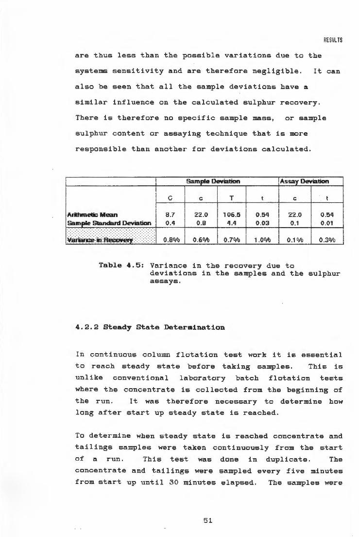
I i

RESULTS

are thus less than the possible variations due to the

systems sensitivity and are therefore negligible.

also be seen that all the sample deviations have a

It can

similar influence on the calculated sulphur recovery.

There is therefore no specific sample mass, or sample

sulphur content or assaying technique that is more

responsible than another for deviations calculated.

Sam De¥iation Assa De¥iation

I ! T C C C

I Alilhmetic Mean

I Sam Standard Deviation 8.7 0.4

22 .0 106.5 0 .54 0.03

22.0 0.1

0 .54 0.01 0.8 4.4

0 .8o/o 0.6°/o 0.7% 1.0% 0.3%

Table 4.5: Variance in the recovery due to deviations in the samples and the sulphur assays.

4.2.2 steady State Determination

In continuous column flotation test work it is essential

to reach steady state before taking samples. This is

unlike conventional laboratory batch flotation tests

where the concentrate is collected from the beginning of

the run. It was therefore necessary to determine how

long after start up steady state is reached.

To determine when steady state is reached concentrate and

tailings samples were taken continuously from the start

of a run. This test was done in duplicate. The

concentrate and tailings were sampled every five minutes

from start up until 30 minutes elapsed. The samples were

51

RESULTS

then weighed and analysed for their sulphur content. The

sulphur grades and recoveries were then plot.t.ed against

time <Figures 4.4 and 4.5 ) and used to determine when

steady state was reached.

The steady state cri t .erion decided upon was that the

sulphur grade and recovery of samples taken at st.eady

state must lie within the 95% confidence interval

determined in section 4 . 2.1 .

60 100 8

s u I u ~ I 40 80

~ 95% Conf ldenoe Boundary u u r r 30 - 60 R G e r 95% Conf ldence Boundary C

0 a 20 40 V d e e r

10 20 y

% Grede Run 4

s -a- % s

0 0 6 10 16 20 26 30

Time when taking Sample (min)

Figure 4. 4: , Sulphur grade and recovery versus time to determine when steady state is reached in the column <Run 3).

From figure 4.4 and 4.5 it can be seen that after fifteen

minutes steady state was reached. This was confirmed by

doing another run <Figure 4. 6) and taking samples every

minute from fifteen to twenty two minutes after start up.

Again the sulphur grades and recoveries were wi t .hin the

95% confidence interval determined.

Although only fifteen minutes were required to reach

steady state it was decided to wait thirty minutes before

taking samples.

52

RESULTS

s u I

R u r

G r a d e

% s

10

0

96% Oonf ldence Boundary 40

20

0 5 10 15 20 25 30

Time when taking Sample (min)

Figure 4.5: Sulphur grade and recovery versus time to determine when steady state is reached in the column <Run 4).

s u I

R u r

G r a d 8

% s

96% Oonf ldenoe Boundary 30 1------------------------ 60

20 40

10 20

0 0 15 16 17 18 19 20 21 22

Time when taking Sample ( min)

8 u I

g u r

R e C 0 V e r y

% s

8 u I

g u r

R e C 0 V e r y

% s

Figure 4.6: Sulphur grade and recovery steady state confirmation for times between 15 and 22 minutes <Run 5).

53

RESULTS

4.2.3 Repeatability

It is important to determine the repeatability of t .he

experimental procedure. Firstly repeatability ensures

that the grade and recovery

variations in the values of

trends observed for

parameters are meaningful.

physical and chemical

Secondly t he grades and

recoveries obtained should be consistently achievable.

50~~~~~~~~~~~~~~~~~~~~--,100 8

s u I

~ u r

(3 r a d e

% s

40 80

30 ----- 60

20 40

10 20

0 0 6 10 16 20 26 30

Time (min)

Figure 4.7: Sulphur grade and recovery versus time to determine the repeatability of the column <Run 3 & 4).

u I

~ u r

R e C 0 V e r y

% s

Figure 4.7 shows the repeatability in the grade and

recovery values over the thirty minutes from start up.

In both runs 3 and 4 the percent sulphur recovery dropped

between five to ten minutes after start up and then

remained essentially constant. The sulphur grades

increased slightly over the first fifteen minutes. For

runs 6 and 7 <Figure 4.8) good repeatability was again

achieved for the grade and recovery trends.

water temperature was varied in runs 6 and 7 .

The wash

The second part of the repeatability study was to achieve

the same grades and recoveries consistently. Two runs

54

RESULTS

were each done for eighty minutes. Figure 4.9 shows the

consistency achieved. The sulphur gradets differed on

average by less than 1% and t .he sulphur recoveries

differed on average by less than 2. 5%.

s u I

~ u r

G r a d 8

% s

60 100

40 80

30 - 60

20 40

10 20

0 0 23 30 41 49

Wash Water Temperature (Degrees Celcius)

Figure 4.8: Sulphur grade and recovery versus wash water temperature to confirm the column repeatability <Run 6 & 7).

8 u I

~ u r

R e C 0 V e r y

% s

It was therefore concluded that the experimental

procedure was adequately repeatability.

4.2.4 Comparison between conventional and column

:flotation.

The reason

conventional

for doing

laboratory

a comparative study

batch flotation cell

of

and

a

a

laboratory column flotation cell is that it is necessary

to determine which type of flotation performs better.

The performance is judged in terms of the concentrate

grades and recoveries obtained.

A difference in the performance is expected because of

the different types of pulp/air contact, the froth

55

RESULTS

60 100

s u I 40 i i ~ 80

~ it

u r 30 60

G r a 20 40 d 8

20 %

10 s

0 0 20 40 60 80 -

Time when taking Sample (Minutes)

Figure 4.9: Sulphur grade and recovery versus time to confirm the column reproducibility <Run 8 & 9).

8 u I

~ u r

R e C 0 V a r y

% s

height and the presence or absence of wash water. An

improved concentrate grade in t .he column flot.ation cell

is expected due to t .he presence of wash water and the

deep froth height.

To test the performance of each flotation system the

column was used as described in the experimental

procedure (Section 3. 2). A batch of the feed sample to

the column was then taken and added directly to the

conventional laboratory batch flot.ation cell to ensure

that identical feed conditions were used. This procedure

allowed the conditioning time and reagent additions to be

identical for both systems.

From the experiments conducted it was found that the

column produced concent.rates with higher sulphur grades,

for similar recoveries, than possible with the batch

cell <Figure 4.10). From Figure 4 . 10 it can also be seen

that the sulphur recoveries were generally higher for the

column . The higher sulphur recoveries obt.ained with the

56

RESULTS

column were achieved at lower solids residence times than

in the batch cell <Figure 4.11).

The column produced a gold concentrate with a grade of

86 g/ton compared to 140 g/ton for the batch cell <Column

run 17 and batch test 1). The gold recoveries for both

methods were however the same. The particle residence

time in the batch cell was 14 minutes compared to the 2.9

minutes in the column.

From a size analysis it was found that the percent fines

reporting to the concentrate (Figure 4. 12) is lower for

the column flotation cell t .han for the conventional batch

cell.

s u I

~

111 Flotation Column

-&- Conventional Cell

GIi

I

u 26 r

Ill ---------------------------------·---·-----Ill

Ill

G r a d 8

% s

201------- ---------------------1

16'----....._ __ _._ ___ ..__ __ _._ __ ___._ ___ .._ __ _._ __ __,

50 65 60 65 70 76 80 Sulphur Recovery (%8)

85

Figure 4.10: Sulphur grade versus sulphur recovery for column and conventional batch flotation comparison <Run 10).

57

90

s u 100 I

~ u 80 r

R e 60 0 0 V

...

8 40 r

-·---I e s 20

% 8 0

0

a

mm Ill Ill l!D a a

D

··---0

a Column Run 10

a Batch Test 1

I I I I I

2 4 6 8 10 Particle Residence Time (minutes)

Figure 4.11: Sulphur recovery versus particle

w e I

~ t

p e r G a n t

10

1

0.1

residence time for column and batch comparison <Run 10).

------------------

Iii Batoh oonoantrata 8

+ Batoh oonoentrate 4

* Batch concentrate 5

a eatch concentrate 6

~ Column Concentrate

RE SULTS

a

__ ,. __

- ·

12

0 .01 L---'----1---1--L-1....I--LJ.~--..L..-L-L...-L_l,_L.L....L...L-----L-J-...L....L--'-L.L-L.I

1 10 100 1000 Particle Size (Microns)

Figure 4.12: Particle size analysis for a column and conventional batch flotation comparison.

58

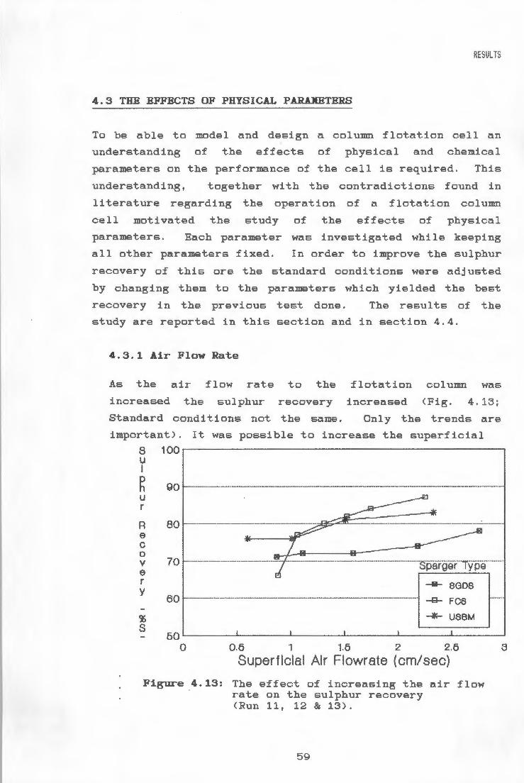
RESULTS

4.3 THE EFFECTS OF PHYSICAL PARAJCETERS

To be able to model and design a column flot.ation cell an

understanding of the effects of physical and chemical

parameters on the performance of the cell is required. This

understanding 1 together wi t.h the contradict.ions fm.md in

1 i terature regarding t.he operation of a flat.at.ion col 1.1mn

cell mot.ivat.ed the st1.1dy of the effect.s of physical

parameters. Each parameter was invest.igat.ed while keeping

all other parameters fixed. In order to improve the sulphur

recovery of this ore t .he standard conditions were adjusted

by ch;:mging them to t.he paramet.ers whic,h yielded t.he best

recovery in the previo1.1s test. done. The resul t .s of t .he

study are reported in this section and in section 4.4.

4.3.1 Air Flow Rate

As the air flow ra.t.e t.o the :flat.at.ion column was

increased the sulphur recovery increased (Fig. 4 . 13 ;

Standard condi t.ions not. the same. Only the t.rends are

important). It was possible to increase the superficial

8 100 ..---------------------------, u I

g 90 u r

R 8 C 0 V e r y

% s

70 .... _ .. _ ........... _ .......................................... -·---·-·-·-.. --·-----.. ------.. ·-·---·-.. - .............. Sparger·· ry pe - ...... -.

-II- SGDS 60 ______ ............... -........... -·-·--··--···--·--·---.. ·----·--··--··---····----·---· -9-- F CS

-+ U8BM

5Q'-~~~ .......... ~~~~..._~~~--'-~~~~_._~~~_.~~~~

0 0.6 1 1.6 2 2.6

Superflclal Air Flowrate (cm/sec)

Figure 4.13: The e:ffect. of increasing the air flow rate on the sulphur recovery <Run 11, 12 & 13).

59

RESULTS

air rate up to 2,5 ± 0,3 cm/sec before slugging occurred.

When slugging occurred the deep froth col lapsed. Optimum

air rates were therefore obt.ained which compare well with

those reported in literature.

As expected, the s1.1lphur grades decreased as the air

rates were increased (Figure 4. 14; Standard conditions

not the same. Only the trends are important.) . An

exception occurred when the USBM type sparger was used.

s u I

~ u r

G r a d e

% s

4 0 ... ·-······-······-·· .. --.....

Sparger Type

-B- 8GD8 1 0 -··--··········-·····-·············-············--···--·--·-·--------------------·---·-·· -9-- F CS

--*" U8BM

o~---~----~----_..__ ____ _._ ____ _.___ ___ __, 0 0 .6 1 1.6 2 2.6

Superficial Air Flowrate ( cm/sec)

Figure 4.14: The effect of increasing the air flowrate on the concentrate sulphur grade (Run 11, 12 & 13).

3

When the air rate was increased the sol ids densi t .y in the

concentrate decreased (Figure 4. 15; St.andard conditions

not the same. Only the trends are important).

The mae.s of fine part.icles reporting to t.he concent.rate

generally increased as the air rate was

(Figure 4.16, 4.17 and 4.18).

4.3.1.1 Sparger Type

increased

When t .he sintered glass disc, sparger, SGDS, is 1.1sed

bubbles with a mean diameter of 1,2mm can be produced.

60

0 0 n 0

s 0 I I d 8

D e n 3 I t y

RESULTS

-3- SGDS

ao~-- -e- FCS

-*"" USBM

6Qt---- ~ar

* * * -

0'-----------...._ ___ _.__ ___ _._ ___ _._ __ ___.

0 0.6 1 1.6 2 2.6

Superficial Air Flowrate (cm/sec)

Figure 4.15: The effect of increasing the air flowrate on the concentrate solids density <Run 11, 12 . & 13).

M 1 a SGDS 8 s Superflclal

0 0.8 Air Rate om/sea)

0 I -+- 0.87 I 0.6 ---8 1.11 C -e- 1.68 t 8 0.4 2.18 d

2.76

g 0.2 r a m s 0

1 10 100 Particle Size (Microns)

Figure 4.16: Particle size distribution for the concentrate when using the SGDS at varying superficial air rates.

61

1000

M a s s

C

RESULTS

3.6 ~~~~~~~~~~~~~!==~~~~~--,

·--------·--·--·····---..S.up.e.r.f.lclaL ___ _ Air Rate (cm/sec)

3 ··········-···············-······-·········-··--·······-··--------·-·-----·---··-·-

0 2. 5 ··········-··-··-----····-·······-·····-···-······-······-·····------·----···-··------·-- -a- 0.88 1 I -+- 1.06 e 2 -*" 1.31 C t -*-e 1.5

1.52

~ d

g r a m s

M a 8 s

0 0 I I a 0 t e d

g r a m s

1

0.5

-----·-··---·---- ~ 1.74

2.25

0 ~ ....... ~~liLLLL---1.--1___L..LL.LLLL---1.--1___L..LLLW

1 10 100

Particle Size (Microns)

Figure 4. 17: Part.icle size distribution for t.he concentrate when using the FCS at varying superficial air rates.

1000

1.4 ,----------------------------. USBM

1 . 2 -··················-···-···················-·······-·--·------------·-------·-------·-·-····-········- ··----··----················81Jperf tntat-····-··-··-

Al r Rate (om/sec) 1 ·····---·····-·--····-···-······-·"······---·-·---··--····--------·--·--- -·· . ---·--···--··---···-···--···-···-········-··-····----

0. 8

0.6

0.4

0.2

0 1 10 100


-+- 1.51

-*" 1.01

-G- 0.60

-x-- 2.33

1000

Figure 4.18: Particle size distribution for the concentrate when using the USBM sparger at varying superficial air rates.

62

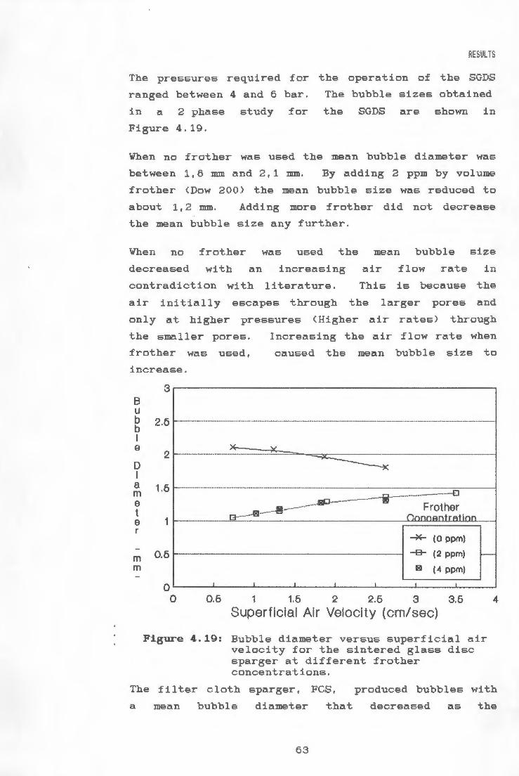
RES llLTS

The pressures required for the operation of the SGDS

ranged between 4 and 6 bar. The bubble sizes obtained

in a 2 phase study :for the SGDS are shmm in

Figure 4. 19.

Vhen no frat.her was used the mean bubble diameter was

between 1,5 mm and 2,1 mm. By adding 2 ppm by volume

frother (Dow 200) the mean bubble size was reduced to

about 1, 2 mm. Adding more :frat.her did not decrease

the mean bubble size any further.

Vhen no frat.her was used t.he mean bubble size

decreased with an increasing air flow rate in

contradiction with lit.erature. This is because the

air initially escapes t .hr01.1gh the larger pores and

only at higher pressures (Higher air rates) thr01.1gh

the smaller pores.

fr other was used,

increase.

Inc,reasing the air flow rate when

caused ·the mean b-ubble size to

B u b b I 9

D I a m e t e r

m m

3~---------------------------~

2. 5 ····-------------··············-····-··--··-····-······-····-------··-·-····-···------·-·--··---··-·-··-··----··-·--·----··-··--··-····-··----·--····-··-··-·-······-··········-··-··--··-··-···

2 -··········-··-··--········-·-·-····-···-·-··············-··------------··

1.5 ~ -------------·j ·--------------------·-··--El

!!------------- F rot her 1 ---------------- G-----s ------- ______________________________ Qonoantrailo.n. __ _

-*- (0 ppm)

0.6 ··-····-----·-··········-------------------------------------- ~ (2 ppm)

® (4 ppm) 0 ...._ __ __._ ___ ...._ __ __. ___ _._ ___ ..__ __ --1.. ___ ..L-__ __.

0 0.5 1 1.5 2 2.5 3 3.5

Superficial Air Velocity (cm/sec)

Figure 4. 19: Hubble diamet.er versus superficial zdr velocity for the sintered glass disc sparger at different frother concentrations.

4

The filter cloth sparger, FCS, produced bubbles with

a mean bubble diamet.er that decreased as the

63

RESULTS

superficial air velocity was increased (Fisure 4.20).

This is in cont.radict.ion with lit.erature. This is

because t.he air initially escapes t.hrough t .he larger

pores and only at hisher pressures (Higher air rates)

through the smaller pores. This is possible due to

the large sparser s1.1rface area available <Ratio of

column cross sectional area to sparger s1.1rface area

equals 1). Adding 4 ppm Dow frot.her res1.1l t .ed in the

mean bubble diameter only decreasing by about 0,1 mm.

The United States, Bureau of Mines type sparger, USBM,

produced b1.1bbles with a mean bubble dii:tmeter of about.

2,3 mm (Fisure 4.21) wit.bout. t.he addition of frot.her

in t .he sparger water. When a froth er, Dow 200, was

added it was possible to control the bubble size and

reduce the mean bubble diameter to about 1 mm.

B u

3~---------------------------~

g 2. 5 ····-··········"-····-·· ······-····--····-····-······-··"··--····-··········-····-··----····-····-··-··-·---------··-···--··-····--··-··········-··-··--· .. ·-······-··---······-··-··-·······-··--··--····--·

I 9

D I a m e t e r

m m

1 . 5 --·-······-··-··---··-··-···-··-···-···-···-·--·····-····--··----··------------··-··-·------·-------··--··-----------··--.. ·-··-··-·-··- ···--··-·-

1 --------- ··-----··-····--·-···---·------------·------·-·-------------··---Prothew·-··--····----··--· Oonoentratf on

0.6 --···-·----··-------··--·---------------------- -*" ( 0 ppm)

-B- (4 ppm)

0'------'----...__ __ __. ___ _._ ___ ..__ __ __,L ___ ~ __ __,

0 0.6 1 1.6 2 2.6 3 3.6


Figure 4. 20: B1.1bble diameter versus superficial air velocity for the filter cloth sparger at different frother concentrations.

4

The st.andard deviation of the bubble diameter

distribution w.:ts smallest. £or t .he USBM. The standard

deviation was abo1.1t 10 times smaller for t.he USBM th;:rn

for the FCS <Appendix B; Run 10 and 11).

64

B u b b I 9

D I a m e t e r

m m

s u I

~ u r

RESULTS

3~--------------------------,

2.5 ········--····· .. ···--······· .. ····· .. ············-·······~ ···---··-·-·-···· .. ··---······-.. -··--···-··-··"-········ .. ---· .. ·-· ......... -.... -........ .

2 ··--·-··-··-·-····-----··-········-··-------·······-·-·--··-·-·--·-·--··---···-·-----·-·-·--------·····---···--······-··-··--····-····-····-··-·-·-··--·-·---·-·-·-···

1 , 5 ----·· .. --·-.. --···-·················-····-···-··-····-··--·------------·-·---·-··---.. --··-.. -··-··-···· .. ----·-·----····-··-··-......... ,_, __________ ... , ............................ - ......... . 181

~ Frother 1 -·-.. -----.. -... -.. --.. -.. -··-.. --··--··~ -··---=--···-----··-····-····-·---..Oo.ncan-t-rat~on ..... ----··

-*- (0 ppm)

0. 6 -.. -·---·--··-···-·-···-·-·-··-···-·-·--··--·-·--·-·----------··---------·------ -8- ( 2 ppm)

-&- (4 ppm)

0 L--__ ...__ __ _._ __ __._ __ __. ___ ...___ __ _.__ __ _..._ __ __.

0 0.6 1 1.6 2 2.6 3 3.6


Figure 4.21: Bubble diameter versus superfic ial air velocity for the United States Bureau of Mines sparger at different frother concentrations.

50r---------------------------,

* * 4 0 ----··-·--··--··--········-·-·--·-····-·····-·-··--··-·-·-------··--------·-··-"*-·--··-·-··--.. ---------···-·---··-·-----··· .. ···-··---··--·-··-

* 30 -···-·········-··-·-------··-··········--··---··---··--- o·-··--··-·----···-··--·-------·o ______ ··--·-···---···---··------····-··-··-··-······-··-····-------··-··----

a

4

G D r D

~ 2 0 ----··-··---------····-··-··-·-··---------------·--··-----·---------------··-·-·-----··--·spar ger iy p e ---·--

e

% s

1 0 -·--··-··-··-·--····-··-··-····-··-----·--··-····------··------··-----·-----------·-··----··-··-·--···-·--·--.. - D F 08

* USBM o...._ _ __._ __ _.___--J. __ _._ __ ..__ _ _..._ __ _.___--J. _ _ _._ _ ___,

50 55 60 65 70 75 80 85 Sulphur Recovery (%8)

90 95 100

Figure 4.22: Comparison oft.he sulphur grade versus the sulphur recovery for the SGDS, FCS and the USBM spargers .

65

RESULTS

Comparing the s1.1lph'ur grades and recoveries obt.ained with

the filter c lot.h sparger,

Bureau of Mines sparger,

FCS,

USBM,

zrnd the United States

it was found that the

USBM produced the best concentrate grades at a specific

recovery (Figure 4 . 22) . The frot.her concent.ration was

not increased further because this increase does not

significantly decrease the bubble size.

4.3.2 Collection Zone Length

By increasing the collection zone length from lm to 4m the

sulphur recovery increased from 84% to 89% (Figure 4. 23) .

The sulphur recovery remained at i!!.ppro:,dmately 89% when

the collection zone was increased to 6m. The sol ids mass

in the concentrate also increased as the c ollection zone

length was increased .

of 4 meters.

The maximum was reached at. a length

In general the concentrate sulphur grade remained constant

as t .he c ollec t .ion zone lengt.h increased ( Fig1.1re 4 , c'. 3 ) ,

There was also no change in the part.icle size distribution

as the collection zone length was increased.

s u I

~ u r

G r a d e

% s

60 .--------------------~ 100 8 u I

90 g

30 -····--------··--······· -··-····--·--·-.. -··---·-, .. ,_ .. ______________ _

2 0 _ ........................ --.. -, .. , .. _, ... _,.,, .. _ .... , ...... _,_ ........ ,_ .. ,, __ ,,, _____ ,, __________ ,,_,,_, ___ .. _ .. _,, _____ .... ,,_,_,,_ .. ____ ,,,,_,,,,,, ___ ,,.. 7 0

1 0 ---.. --....... _ .. _____ .. _______ .. ________________ ,,________ _g.... Aeoover y ·-- 60

-&- Grade

o~--~--~--__._ __ _._ __ ___..__ __ _._ _ __j5o 0 1 2 3 4 5 6 7

Collectlon Zone Length (m)

Figure 4.23: Sulphur recovery and grade versus collection zone length <Run 14).

66

u r

R e 0 0 V e r y

% s

RE SULTS

4.3.3 Cleaning Zone Depth

The most obvious effect of increasing the c leaning zone

depth was that the sulphur recovery decreased

<Figure 4 . 24) . When the froth depth was increased from

25 cm to 100 cm the recovery decreased from 83% to 73%.

s u I

R u r

G r a d 0

% s

60

40

30 ~ -~ =======

20

10

0 0

I

26

-e- Recovery

-8- Grade

I I I

60 76 100

Froth Depth (cm)

100

90

80

70

,_ 60

50 126

s u I

g u r

R e C 0 V e r y

% s

Figure 4.24: Sulphur recovery and grade versus froth depth <Run 15).

Unlike the improvement in

reported in literature,

concentrate

it was

grades that were

found that the

concentrate sulphur grades remained constant and then

increased slightly at a depth of 75 cm <Figure 4.24). At

a froth depth of 100 cm the sulphur grade decreased

again.

From Figure 4.25 it can be seen that the amount of larger

particles reporting to the launder increase with a

decreased froth depth.

67

w e I

R t p e r C 8 n t

100

10

,__ .....

RESULTS

·-->-··----·------------ ------------------

~----------------------··-------------------! ... J

.... "i_· .,.

..... ·------•!IIIICIJ------·--·------·--------------·--

r "' 1,-. - - -·----·~·~ E:- . .. ---- F==·----------·------::----=:..=:a~~-""-

.. -+- -100 -~ 70

~ -e- 50

J!

r 0. 1 i=.. ..-, - ----- _ -------=:=---======================-===l ""'" ---------------·-------·--·----

"'*"" 25 --I I I I I I I I 0.01 L..-_ __._1 _...,_1__.1__._1 _.1 ..... ._1._11..,1 ___ .__,_..1..-•..1.•-.L..L••...L•.....1•...L•..1.• __ .....a___J..__L-1-L...L..J...J..J

1 10 100 1000 Particle Size {Microns)

Figure 4.25: Particle size analysis for varying cleaning zone depth .

4.3.4 Feed Solids Percent

As the feed solids percent. was increased the sulphur

recovery decreased minimally up to a solids density of

25, 3%. When the feed solids density was inc reased to

38 , 4% the sulphur recovery dropped dramatically to 59%

<Figure 4.26).

The sulphur grade increased and then reached a maximum as

the solids feed rate was increased (Figure 4.26).

By increasing the

solids collected

larger

feed solids density the mass of the

increased in all size ranges . The

particles collected was decreased percent

slightly. At a :feed solids density of 38,4% however,

the mass o:f larger particles

drastically <Figure 4 . 27).

68

collec ted decreased

s u I

~ u r

G r a d 8

% s

M a 8 s

C 0 I I e C t e d

g r a m s

RESUL TS

60 100 8 u

-G- Recovery I

40 --- Grade 90 ~ u r

30 -- 80 R e C

20 70 0 V 8 r

10 60 y

% s

0 50 0 6 10 16 20 26 30 36 40 46 60

Feed Solids Percent (% mass/mass) Figure 4.26: Sulphur recovery and grade versus feed

solids percent <Run 16) .

2.--------------------------,

Percent Sol Ids Feed 1.6 ---·--- -·------------oensny -{mass7mass1

~ 8.7

11------ -+- 16.Q

-A- 26.3

~ 38.4

0.61-----

0'---~~...__.._---'-...L..L..L.LL---_._--L--L---L.....L..L..L.LL---_.___.___.___,__..L...L..._._,

1 10 100 1000 Particle Size (Microns)

Figure 4.27: Particle size analysis for a varying feed solids density.

69

RESULTS

4.3.5 Volumetric Feed Rate

Increasing the volumetric feed rate from about 800 ml/min

to about 2000 ml/min while keeping the percent solids

constant at 10% solids had virtually no effect on t .he

sulphur recovery. The

77% to 80% <Figure 4 .28).

sulphur recovery increased from

The largest increase (2%) was

found when the volumetric feed rate was increased from

800 ml/min to 1000 ml/min,

were not significant. while the other increases

The sulphur grade also remained essentially constant. A

possible opt.imum in grade can be seen at a volumetric

feed rate of 1600 ml/min <Figure 4.28).

s u I

~ u r

G r a d 8

% s

60

40

30

20

10

0 600

- ----- -- --- -- -

-a- Recovery

-II- Grade

I I

1000 1600

Volumetric Feed Rate (ml/min) '

100

90

s u I

~ u r

-- 80 R ~

-- 70

- 60

50 2000

e C 0 V e r y

% s

Figure 4.28: Sulphur recovery and grade versus volumetric feed rate <Run 10) .

Increasing the volumetric feed rate increased the weight

percent of larger particles collected in the concentrate.

At a volumetric feed rate of 1958 ml/min the weight

percent of larger particles

drastically <Figure 4.29).

70

collected decreased

RESULTS

20 w

Volumetric e I Feed Rate (ml/min) g h 841 t

-t- 1010 p

4- 12Q2 e 10 ----r -e- 11578 C 8 1726 n

1958 t 6

%

0 L..--__._---=-_.__ ................................ .___ _ __,__..,__..J.-...___._,_........_. __ -W,-_..__..,__ ......... ...L..I..J...J

1 10 100 1000 Partlcle Size (Microns}

Figure 4.29: Particle size analysis for a varying volumetric feed rate.

4.3.6 Wash Water

4.3.6.1 Wash Water Rate

The sulphur

<Figure 4.30)

210 ml/min.

recovery

at. a

passed through

wash water rat.e

an optimum

of about

The concentrat.e sulphur grade decreased as the wash

water rate increased from 118 ml/min to 212 ml/min

<Figure 26). A further increase of the wash water

rate to 355 ml/min caused the concentrate sulphur

grade to increase again.

Increasing the wash water rate from 118 ml/min to

137 ml/min increased the mass of t .he coarse particles

collected (Figure 4.31) .

'71

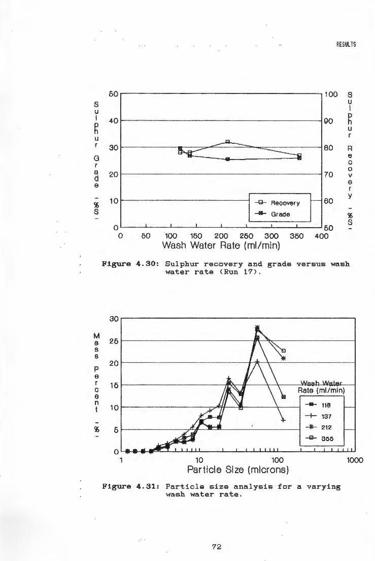
s u I

~ u r

G r a d 8

% s

M a s B

p 8 r C 0 n t

%

RESULTS

60

40

30

20

10

0 0

100

90

G---:::::::: ~ 80

-- 70

-a- Recovery r- 60

-&- Grade

I I I I I I J 50 60 100 160 200 260 300 360 400

Wash Water Rate (ml/min)

8 u I

~ u r

R e C 0 V 8 r y

% s

Figure 4.30: Sulphur recovery and grade versus wash water rate <Run 17).

30

26 ---

20

16

10 --- 118

-+- 137

6 -*- 212

-Q- 300

0 1 10 100

Particle Size (microns)

Figure 4.31: Particle size analysis for a varying wash water rate.

72

1000

RESULTS

4.3.6.2 Wash Water Position

Lowering the wash water position from 5 cm to 20 cm

below the concentrate overflow level did not affect

the sulphur recovery or grade <Figure 4 . 32). The only

effect that lowering the wash water position had on

the column operation was that the percent. solids in

the concentrate was increased and then reached a

maximum.

The particle size distribution did not. change at all

as the wash water position was changed <Figure 4.33).

s u I

~ u r

G r a d a

% s

60 100 8 u I

40 - 90 g u r

30 80 R ~= : : e C 0

20 -- 70 V a r

10 1--....g.... Recovery 60 y

-II- Grade % I I I I I I I I I I I I s

50 0 0 2 4 6 8 10 12 14 16 18 20 22 24

Wash Water Position (ml/min)

Figure 4.32: Sulphur recovery and grade versus wash water position <Run 18).

73

w 8 I

~ t

p 8 r C 0 n t

100

RESULTS

--- . r"'"' ----------·------------------------------------

-1 0 E==--- ··-··---:-··- --= --

- --~ ----------·------------ -· v- ------·-·--·----·--------·-------··----·----·-----·-- ~ -------------------·----·-------·----··-·

\ _ .... == - ··~ --- -- ......_ - 6 om -

_ _____ ,_r ___ _________ _

I

-+- 10 cm E --=

I 0.1 ~-

4- 15 cm -- ·----.... . .__ i---------- ------------i -Q- 20 cm

I----0.01 1...-_ __,1.l_.....11~11--11-.L I.J....J. 11..._ I..,__ l _ __.1 _ __,1.__ .......... 11 ...... ......._ II ...._I..._ I...._ l _ __.1 _ __,1.__ .......... 11_..._ 1........._ II_._. I

1 10 100 Particle Size (microns)

Figure 4.33: Particle size analysis for a varying wash water position .

1000

4.3.6.3 Wash Water Temperature

The wash water temperature was increased from about

21°C to about 50°C . This decreased the sulphur

recovery marginally while the grade increased by about

4% <Figure 4.8).

At higher wash water temperatures more particles

larger than 100 microns were collected . This is

clearly shown in Figure 4.34.

4.3.7 Feed Position

In the laboratory tests the feed position was lowered

from 55 cm to 85 cm below the concentrate overflow while

keeping the froth depth and t .he collection zone depth

constant. The sulphur recovery decreased slightly while

the concentrate sulphur grade improved (Figure 4 . 35) .

74

w a I

R t p e r C 8 n t

s u I

~ u r

G r a d a

% s

RESULTS

10

0.1

o.01 .__ _ __,____..___.._._ ..................... ..__ _ _.___.___.__,_.._._ ........... __ _.___.___._.....__L..L.JL..I..J

1 10 100


Figure 4.34: P~rticle size analysis for a varying wash water temperature .

60 100

40 90

30 ..... a= - iif=='"" -=-::::::::::8 80 a-- 8

---0

20 ...... -- 70

10 ....Q- Reoovery t- 60

--- Grade

I I I I I I I I I 0 60 60 66 60 66 70 76 80 86 90 96 100

Feed Position {cm)

1000

8 u I

~ u r

R e C 0 V e r y

% s

Figure 4.35: Sulphur recovery and grade versus feed position <Run 19) .

75

I i I I i

RESULTS

4.4 THE EFFECT OF CHEMICAL PARAMETERS

4.4.1 Leaching the ore

The pulp w;:,.s leached for 3 hours at a pH of 3. 8 and t .hen

it was floated at. t .he same pH to determine what. the

effect was on the sulphur recovery.

As a result of the lowered pH the sulphur recovery

increased from about t .o 88% ( Run .20). The

concentrate s1.1lphur grade however decreased from about.

22% to about 20% sulphur when the pH was lowered.

4.4.2 Conditioning Procedure

By increasing t .he conditioning time from about 25 to 30

minutes it was possible to increase the sulphur recovery

I

I I !

I Run18 I I Run 19 I

I Run22 I I Run14 I

Run 18 1 ~ -c t'Wl'ii.s J

I I I

Run22 i Run14 I

i

j

Solids I Frnther \.'I/ash Jg Sup. Go!!. Froth I I Height Height ! Feed

I Addition \!'later Bias

! Rate Rate Rate ! C.1"11 C.:'511 ! gl111in I g/ ton 111 l/)11 in 0111/ s@c cm.ls@c

I I

I

225 25 ! 17.C "1?7 200 1.0 0 .13 i l" tY I

225 25 ! 17? 136 200 1.0 O.i'.3

I 225 25 1rn r:J7f'I 200 1 .5 0.{}7 Dv I -·v

230 25 ! 171 ! 137 200 1 .9 0.12

Sparger S!PX A.FLT Goncl. I Sulphur

l Sulphur

Type Addition Addition Time ! Recovery Grade Rate Rate !

I I I ,..../; .-,,,.,. ,.... .r., - ~, .:'11it1 %S I %S 5 ·' ~!...·.:.: 5 .· ~:..·.:.:

FCS 23 38 25 73 25 FGS 22 37 30 76 30

FGS 26 44 30 85 22 .5 FCS .. !J •~ 30 10+10 85 30

Table 4.6: Details for different conditioning times and procedures.

76

RESULTS

from 73% to 76%. At the same t.ime the concentrate

sulphur grade was increased from 25% to 30% (Table 4.6).

It was observed that. by adding t.he reagent.s step wise it.

was possible to increase the S'l1lphur grade by 5% while

keeping t .he recovery canst.ant. at 85% <Table 4. 6). This

total improvement was possible even t.ho'l1gh the

conditioning time was reduced and only '70% of the reagent.

dosage was used.

4.4.3 Collector Dosage

By increasing the collect.or dosage the sulphur recoveries

and the sulphur concent.rate grades improved

significantly.

An increase in reagent. dosage from about. 10 g/t.on to

120 g/ton improved the sulphur recovery from 52% to 84%,

while t .he sulphur grade improved from abm.1t. lf1% to 26%

<Figure 4.36).

s u I

~ u r

G r a d e

% s

60 .------------------------, 100 8 u I

4 0 ----------···-·---------- --------- 90 g u r

a::==-a-==:::::::=== -----··---------------·--··-- 80 R

70

10 -G- Recovery -- 60

-II- Grade

0'----'----'-----'-----'-----'-----L--~50 0 20 40 60 80 100 120 140

Collector Dosage, SIBX ( g/ton)

Figure 4.36: Sulphur grade and recovery versus collector dosage (Run 21).

77

8 C 0 V e r y

% s

RESULTS

As the collector doe.age was increased the mass percent

particles plus 100 microns collected increased

<Figure 4. 37).

60

M a 40 s 8

p 30 Oott9et 9 Dosage ( g/ton) r 0 -a- Q.8 8 20 n -+- 21.7 t

-+- 42.2

% 10 -G- 60.7

-*- 121.(5

10 100 1000 Particle Size (microns)

Figure 4.37: Particle size analysis for an increasing collector dosage.

4.4.4 Frother Dosage

The frother doe.age was increased from

113 g/ton. At 30 g/ton frother addition

recovery was 81%. At frot.her addition

30 g/ton t .o

the sulphur

rates above

57 g/ton the sulphur recovery remained constant at 85%

<Figure 4. 38). The concentrate sulphur grade did not

vary with increasing frother addition.

78

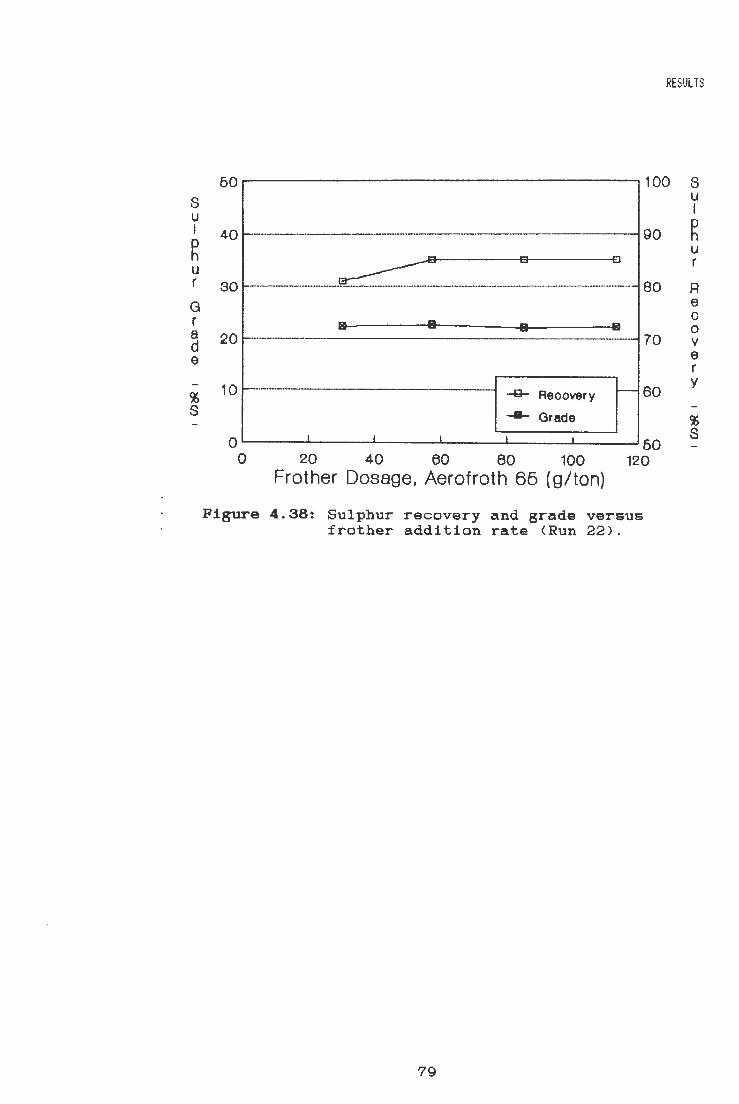
RE SULTS

60 100 s s u I

~ u r

G r

40

30

a 20 d e

% s

10 -·

0 0

90 - - -- -

-- 80

a- II Iii lii'I -- 70

-G- Recovery - 60 ~ Grade

I I I I I 50 20 40 60 80 100 120

Frother Dosage, Aerofroth 65 ( g/ton)

Figure 4.38: Sulphur recovery and grade versus frother addition rate <Run 22).

79

u I

R u r

R e C 0 V e r y

% s

RESULTS

4.5 SUJIXARY OF THB EFFECTS OF P.A.RAJIETERS VARIED

The effects of physical and chemical parameters are

summarised in Table 4. 7. The table also includes a number

of other changes recorded <Appendix D) as a result of

varying physical and chemical parameters.

The following symbols were used in table 4.7

I

I I

D

DD

OPT

MIN

i

I FGS Air Rate I SGDS Air Rate I USBM Air Rate

I I Colect Zone Froth Depth

Feed ~ Solids WIN Rate W!NTemp

1WH1Deplh I I 1vo1 Feed Rate jFeedDepth

I I Golecl Dosage I Frother Dosa

= No change

= Small

= Large

= Small

= Large

= Value

= Value

II I 00 I II

I gg I II

- I - I

- I II I I I

-1 ~~ I I

I = I I - I I DD I -

- I -- I II I

DD I

increase

increase

decrease

decrease

passes through an optimum

passes

-

II D

D

DD D

-

DD

DD DD

I II

I -I -

D

I I -

through a

I 1 DD

I DD I DD

i OPT I MIN

I - I II

I * II I I - I D

I - I

I ~ I -I -

i I D

minimum

I II I II

II I II I I

I OPT I

DO

II

1, ~ II

I I -

OD

* Increase at maximum carrying capacity .

II DD II DD

I OPT

MIN D

D I D

D I

Table 4.7: Su~ry of the effects of physical and chemical parameters.

80

I

II II

DD

D

0

D

D

DISCUSSIOIS

CHAPTER FIVE

5.1 COLUJOI' VERSUS BATCH FLOTATIOI

The column flotation cell was capable of producing sulphur

grades 5 % great.er than those obtained in a conventional

laboratory batch cell at similar recoveries. The column

also achieved up to 15 % higher sulphur recoveries than the

batch cell at similar grades. The residence times for the

column were about 2 minutes compared to the 11 minutes that

were required for conventional flotation to achieve similar

recoveries.

The better concentrate sulphur grades produced by the column

flotation cell were due to the better cleaning effect of the

deep, water washed froth. The superior cleaning also

reduced entrainment into the concentrate launder, since less

(see figure 4. 12) of the minus 10 micron particles, which

are usually entrained instead of being collected by

attachment, were collected. A more selective flotation of

81

DISCUSS IONS

the finer size fract.ions <51. 1 % sulphur was contained in

the minus 38 µm size fraction) therefore resulted in bett.er

sulphur grades.

The improved recovery achieved with the column flotation

cell is due to the particle-bubble counter current contact

mechanism, the wash water and the control over the bubble

sizes . The advantage of the counter current contact

mechanism is t .hat any hydrophobic particles that are not

immediately attached to a bubble have t .he opportunity to

attach the:m6el ves to a clean bubble further down the column

without competing against other more hydrophobic particles.

The wash water washes most fine (minus 10 µm) particles that

tend to be entrained, out of the froth, while with a

controlled bubble size the bubble surface rate can be

optimised to yield an optimum recovery.

The column flot.ation eel 1 is thus significantly better than

the batch cell both in terlD6 of kinetics as well as sulphur

grades and recoveries obtained for the Unisel ore used.

Another attractive feature is the possible reduction of

capital outlay (when installing flotation columns versus

conventional flotation cells) and a reduction of operating

costs .

The improved performance with the flotation column cell

confirmed reports in literature. The column is . therefore an

attractive alternative to conventional flotation and should

always be considered as an option.

82

DISCUSSIONS

5.2 THE EFFECTS OF PHYSICAL PARAJIETERS

5.2.1 AIR FLOW RATE

As the air flow rate was increased the sulphur recovery

increased until an optimum was reached. This was true

for the three types of spargers tested. The increased

recovery due to an increased air flow rate was the

result of a larger percentage of the solids being

recovered in the concentrate. The experimental results

<Table 4.7) prove that the main reason for an increased

sulphur recovery, when increasing the air flow rate, was

due to an increased mass pull. The sulphur grade

decreased but the sulphur recovery increased further.

The question now arises as to how the increased air flow

rate increased the percentage solids recovered. The

answer is that the increased air rate increased the

superficial bubble surface area which in turn increased

the concentrate solids removal rate (increased mass

pull).

When the filter cloth sparger, t .he sintered glass disc

sparger (at O ppm frother) and the USBM sparger (at. 0

ppm frother) were used <Figure 4.19, 4.20 & 4.21) the

total superficial bubble surface area was increased

which allowed more particles to be collected. The

superficial bubble surface area increased with an

increased air flow rate when the bubbles produced by the

spargers became smaller in diameter (Figure 4 . 19, 4.20,

4 . 21) .

An increased superficial bubble surface area will also

be obtained when the bubbles do not increase in size,

but in numbers. Similarly, when the USBM sparger and

the sintered glass disc sparger (at O ppm frother) were

used, the number of bubbles produced did not decrease

<viz. no coalescence of bubbles) but the mean bubble

83

D 1 SCUSS JONS

diameter was increased instead <Figure 4.19 and 4.21).

This resulted in an increased superficial bubble surface

area.

The increased concentrate sol ids removal rate with an

increased air rate or decreased bubble size is confirmed

by the carrying capacity model published by Espinosa

Gomez, et al <1~188). There is however a limitation to

the maximum amount of solids t .hat will float, and to the

maximum superficial bubble surface rate that can be

obtained.

Besides the increased concentrate solids removal rate

experienced due to the increased air rate, the

following two effects also increased the percentage

solids recovered:

Firstly, the bubble residence time in t .he froth, and

therefore the floated solids residence time in the

froth, t1'•·ot.,t, <Table 4.7) was reduced, allowing more

of the less hydrophobic and also more finer particles

<Figure 4.16 to 4.18) to pass into the launder.

Secondly, the collection rat.e was increased

<kc= 1.5-J~Ekdt:,- 1 ) by an increased air rate and a

decreased bubble diameter.

When the air flow rates were increased further slugging

occurred. The flotation process thus ceased to exist.

The maximum in the recovery obt.ained was due to the

following reasons. The total superficial bubble surface

decreased rapidly when bubbles coalesced <causing

slugging), decreasing the concentrate sol ids removal

rate. In the collection rate equation,

k = 1,5-v,;;,-E...,/dt:,, it. is shown that the collection rate

decreases when the bubble size increases. When slugging

occurs this then becomes the overriding parameter.

84

DISUiSSIDNS

In the experimenti:'i.l work the optimum air rat.es were about.

2, 5 cm/sec :for t .he best sulphur recovery. These air

rates compared well to optimum air rat.es reported in

literature (Between 1.7 and 2.5 cm/sec).

The sulphur grades were generally observed to decrease as

the air flow ri:\t.es were increased. This was due to a

higher percent.age solids being collected, This decrease

in grade was also reflected in the increased dilution of

the concentrate and therefore more fines (minus 50

microns) were collected. Alt.hough 60.5 % of the sulphur

was in the minus 53 JJ.m size fraction,

entrain the gangue particles.

higher air rates

Increasing the air :flow rate to its m.:tximum, without the

bubbles coalescing or the n1.1mber of tn.1bbles produced

reducing, will be t.he best opt.ion as far as the recovery

is concerned. In the 1 i t.erat.ure this optimum air ri:\t.e

was recorded t.o be bet.ween 1. '7 and cm./sec. The

concentrate sulphur grade may however be 1 imi ting if the

wash water rate or the froth depth cannot 1:,e increased

enough to achieve an adequate grade.

From the results for increased air rates it was observed

that t.he concent.rat.e grade decrea.sed proportioni:'i.lly to

the concentri:\t.e sol ids densi t .y . The percent.i:\ge sol ids

density can therefore be 1.1sed to estimate the concentri:'l.te

grade for this ore, and maybe for some other ores.

5.2.2 SPARGER TYPE

The USBM type sparger produced the best concentri:'l.te

grades at i:\ specific recovery. The better grades are due

to a better clei:lning i:lction. ( The slightly different.

reagents used for these test do not significantly affect

the the resul t.s. This is shown in table 4. '7. The

physical paramet.ers influence t.he sulphur recovery and

grade much more than the chemical parameters).

85

DISCUSSIONS

The superior cleaning a c tion of the froth, when using

the USBM type sparger, is due to s:maller but,bles

beinggenerated with the USBM type sparger. The smaller

bubbles in t .he :frot.h c ause the :froth to be more stable,

allowing the froth to be better washed.

Turbulence in the froth can be

bubbles are only produc ed in a

column instead o:f being evenly

whole cross sectional area of

worsened if larger

:few sections of the

distributed over the

t .he column. It. is

therefore desirable t.o prod1.1ce bubbles with as narrow a

size distribution cu:. possible . Any t .urt,ulence in the

froth d1.1e t .o t .he rising bubbles ( or wash water) should

be :minimized.

5.2.3 COLLECTION ZOHE LENGTH

By increasing t .he c,ollection zone lengt.h t.he recovery

increased up to 89% and then remained at. abo1.1t. this

value. The increased recovery was due to an increase in

the solids residence t .ime available for particle-bubble

attachment.

The recov•ery inc reased up to 8 9 % and then remained

fairly canst.ant. d1.1e to an equili bri 1.1m being reac,hed

between t .he b1.1bble-particle

bubble-particle separation

cleaning action. If the

attachment. rate and

in the froth due to

recovery zone length

the

the

is

increased after t .he maxim1.1m in recovery is reached any

collected part.icles that. are less hydrophobic <slower

rate constant) and are not attached firmly to the bubble

will thus be washed out of the froth. This was

confirmed by t.he increase in the sulphur grade at a

collection zone of 6 meters, and by t .he :fact. t .hat the

mass of solids collected remained constant after the

:maximum recovery was obtained.

Therefore, unlike conventional :flat.at.ion where an

increased residence time increases the recovery while

the grade is decreased, the :flot.ation column can

86

DISCUSS IONS

maintain a superior grade (above conventional flotation)

with an increased residence time due to the deep froth

and the washing water.

5.2.4 CLEAIIIG ZOIE DEPTH

It is hypothesised that as t .he cleaning zone depth is

increased the time for cleaning is also increased. The

probability that particles are entrained or hydrophobic

particles are collected in the concentrate are thus

reduced. The grade is t .herefore expected to . improve.

The results from the laboratory test work <Figure 4.24)

showed t .hat the concentrate grade increased up to a

froth depth of 75 cm. When the froth depth was

increased to 100 cm the grade decreased. The reason for

this dec,reased concentrate grade is due to the froth

becoming unstable. At the same time the cleaning action

was reduced due to bubble coalescence.

The recovery decreased with an increased frot.h dept.h.

This decrease in recovery was due to the better grades

obtained with a froth depth of up to 75 cm. At a froth

depth of 100 cm the recovery decreased furt.her due to

the froth being unstable and the bubbles coalescing.

Another factor which influenced the decreased recovery

with a deeper cleaning zone was that fewer large

particles report to the concentrate <Figure 4.25). This

was also reported by Debby and Finch (1990).

The increase in grade due to an increased cleaning

action is well recorded in literature and was confirmed

by the test work. An unstable froth was only reported

by Ynchausti and co-workers (1988) for a :manganese

system. Froth instabi 1 i ty is usually due to a lack of

water or solids in t .he froth and can be overcome by

increasing the wash water rate and by adding frother to

the wash water.

87

DI SC:USS iONS

For column flotat.ion operat.ions the cleaning zone depth

can be adjusted to control the concentrat.e grade, An

improved grade will however reduce the recovery.

5.2.5 FEED SOLIDS PERCERTAGE

When the feed solids percent.age was increased the

sulphur

<Figure

recovery remained nearly constant. at about.

where

72%

4.26) 1.mt.il a point. was reached the

sulphur recovery decreased dramatically t .o 59%. The

grade remained more or less constant at 18 to 19%

sulphur.

Increasing the :feed

all other parameters

sol ids percent.age,

constant, did

while keeping

not affect the

recovery and the grade significantly beC:a1.1se the

particle residence t.ime did not vary. The recovery

suddenly decreased i':\S t.he :maxim1.1m ci:lrrying capi:ici t .y was

reached. This was due to the froth becoming overcrowded

which rei:ml ted in t .he larger part.icles (abo1.1t. 35 J.l.m)

being washed out of the frot.h. This phenomenon was

clearly illustrated in figure 4.28.

In the experiments conducted the decrease in recovery of

large particles was proof that. t .he ~ximum c,arrying

capacity was exceeded. To determine t .he maximum

carrying capacity for a specific £lot.at.ion condition,

the feed solids perc,entage can t.h1.1s be increased while

all other parameters are kept constant.

5.2.6 VOLUJIETRIC FEED RATE

By varying the vol 1.1met.ric :feed rat.e t .o t .he flotation

column an optimum performance in t.erms of E-ulphur grade

was achieved. It. can be hypothesised t .hat. the increased

feed gives rise to a higher hydrophillic solids rate in

the froth which in turn stabilises the froth. The more

stable froth is more suitable to an even washing effect

88

DISCUSSIONS

At vol umet.ric £eed rz-tt.es that. are too low the froth mz-ty

become unstable due t.o not. enough part.icles, t,eing

present to stabilise t.he froth. The grade can therefore

decrease d1.1e t.o short. circuiting in an unst.able froth

<Goodall and a~connor, 1991).

In t.he laboratory tests t.he maximum carrying capaci t.y

was just. about. reached because larger particles (Larger

than 30 microns) were lost. t.o t .he tailings inst.ea.d of

being floi:\t.ed (Fig1.1re 4 . 29). There was no loss in

recovery yet. When t.he :froth becomes overcrowded t.he

larger part.icles are washed out. of t.he froth. This was

also not.iced

increased.

when t.he £eed solids percent.age was

If the vol umet.ric feed rat.e is however increased wi t.hout.

the maximum carrying capaci t.y 'being reached, ·t:.he

particle residence time in t.he collect.ion zone may be

decreased t .o such an extent. that. t.he reco~?ery wi 11 be

inhibited.

5.2.? WASH WATER

By increasing t.he wash water rat.e from 118 to 355 ml/min

the recovery passed through ;,.n optimum at. 212 ml / min

while t .he gri:i.de decreased :from i:i.bout. ::;o % sulphi.ir t .o

about 26 % sulphur.

The wash water, as t.he name suggests, has the function

of washing the collected particles int.he cleaning zone .

The decrease in t.he s1.1lphur grade wi t .h Z'tn increased wash

water rate can only be explained as follows. At. low

wash water rates < 118 and 137 ml / min ) it. was visually

observed that t .he wash water had a stabilising effect. on

the cleaning zone. Because the clec"tning zone was st.Z"tble

the cleaning action of the wash water WZ'ts producing high

sulphur grz-tdes. When t.he wash water was increz-tsed t.he

cleaning effect. should have been increased. It. is

postulated however that. the higher wash water rat.es

89

caused the froth to be turbulent,

reduced cleaning action of the froth.

DISCUSSIONS

resulting in a

Changing t .he wash water position had no effect on the

recovery or grade. It did however have an influence on

the water recovered in the concentrate. By lowering the

wash wat.er position the froth above the wash water

distributor has more time to allow the water to dndn

out of the froth.

The position of the wash water distributor can therefore

be varied to obt.ain a concentrate wi t .h a higher solids

density, thus reducing the dewatering capacity required

downstream of the flotation circuit.

An increase in the wash water temperature did not affect

the sulphur recovery significantly <Figure 4. 8). The

sulphur grade did however increase by 4%. This increase

was related to an increased solids density in the

concentrate. The increased wash water temperat.ure

decreased the viscosi t .y and therefore more wash water

was drained from the cleaning zone which resulted in

more fine entrained particles being washed out of t.he

cleaning zone. Wash water with a higher t .emperature

therefore also resulted in an increased solids density.

5.2.8 FBBD POSITIOI

sulphur

The

zone

grade

sulphur

length

By lowering the feed position t .he

increased while the recovery decreased.

recovery decrease is due to the collection

being decreased and the column above the feed point

acting as part of the cleaning zone. The sulphur grade

increased because of the collection zone above the feed

point acting as a cleaning zone and thus preventing any

entrainment into the froth.

90

DI SCUSSIONS

5.3 CHRXICAL P.ARAJOITBRS VARIBD

5.3.1 Leaching the Ore

The ore was leached for 3 hours at a pH of 3,8 in order

to investigate to what extent the flotation perfor:llDnce

could be affected as a result of slight oxidation . The

3 % increase in sulphur recovery and 2 % decrease in

sulphur grade observed was not considered significant

enough to warrant using a lower pH in the investigation .

This increased recovery does however correspond to

reports by Gaudin (1932).

5.3.2 Conditioning Procedure

Increasing the conditioning time by 5 minutes improved

the sulphur recovery and grade by 3% and 5%

respectively. Since the research was mainly focused on

the effect of physical variables on the column

performance no further investigation was carried out on

the conditioning time.

It should however be noticed that by conditioning the

ore in stages it was possible to increase t .he grade

while the recovery remained constant. The reagent

consumption was also lower by using staged conditioning.

The conditioning procedure can be of great importance

and the good resul t .s obtained warrant future research

into this field.

5.3.3 Reagent Dosage

As expected the sulphur recovery increased as the

collector addition rate was increased. At the same time

the sulphur grade increased. This once again

illustrates the fact that the correct collector addition

rate is of great importance.

91

DISCUSSIONS

An increased frother dosage did not affect the sulphur

recovery or grade . Only at a low frother dosage did the

recovery decrease slightly d1.1e to the froth becoming

unstable. The function of the fret.her is to keep a

stable froth and to control the bubble sizes.

During the t .est.work a high fret.her concentration was

used so t .hat a stat,le froth was produced. The higher

frother concentration did not have an effect on the

sulphur recovery and grade and therefore did not affect

the investigation of the physical parameters.

92

PLABT TRIALS

Plant trials were done at the Buffelsfontein Gold Mine.

CHAPTER SIX

These

trials motivated the design and commissioning of a portable

pi lot plant flotation column. The aim was to run the column

in a rougher, cleaner and rougher-scavenger mode and to

evaluate the effect of varying parameters such as wash water

rate, air flow rate, mean liquid and solids residence time

and the solids feed rate.

6.1 PILOT PLABT FLOTATIOI COLUJOI' DBSIGI

Pilot plant flotation column trials have numerous advantages

in that the tests can be carried out at conditions as close

as possible to the actual flotation plant conditions. The

pilot plant column can be run in parallel to the existing

flotation plant making direct comparison possible. The feed

chosen for the column does not need additional treatment as

is often the case in laboratory flotation tests. The

flotation column can also be run continuously for much

93

PLANT TR iALS

longer than in the laboratory . It was thus decided to

design a pilot plant flotation column.

At the outset it was decided to design a pilot plant

flotation column which was:

1) transportable;

2) self supporting with regards to compressed air and water;

3) designed for quick and easy assembly;

4) capable of running as 2 columns in parallel or in series ; and

5) capable of running continuously from a holdup tank and making use of a conditioning tank .

To make the flotation column transportable every part of the

flotation column rig had to be made small and compact. The

water rotameters, air rot.ameters and the level controller

were placed into a single control unit (Figure 6.1).

Figure 6. 2 shows the quick release joints of t .he flot.ation

column enabling ·t.he column to be disassembled into 1. 5 m

sections. The holdup tank, water tank and condi t .ioning

tank can be placed into each other to save space in transit.

A c,a bi net was llll\de to transport t .he slurry pumps and to

provide protection .

To make the pilot flotation column self supporting a

portable compressor and high pressure water pump was bought

<Figure 6.3). The only service required was a 220 V power

supply and potable water .

The facility of being able to assemble and . disassemble the

flotation column quickly was c onsidered important. The

column sections all had quick release .joints and ·- clip on

brackets <Figure 6.2) for quick assembly. The air and water

tubes were all connected with quick release connections

<Figures 6.1, 6.2, 6.3 & 6.4).

94

To be able to run 2 columns,

duplicated <Figures 6.3, 6 . 4 & 6.5).

the high press'\.1re water pump was

PLANT TRI ALS

the control unit was

The air compressor and

used for both columns

simultaneously. The pilot flotation column rig also

included a holdup tank with mixer, a metering pump to add

reagents and a conditioning tank.

95

PLANT TRJ ALS

Figure 6.1: Contro l Unit

Fig 6.2: Quick release joints F1g 6.3: Pilot plant equipment

96

PLANT TRIALS

Figure 6.4: Pilot column launder

Figure 6.5: Complete pilot plant

97

PLANT TRIALS

6.2 EXPERIJIBITAL PROORAX

The plant trials were carried out over a period of two weeks

at Buffelsfontein Gold Mine. The layout of the pyrite

flotation plant is shown in Figure 6. 6. Details for the

pyrite floatation plant are given in Table 6.1. The values

given are the averages for the 7 months between January 1989

to July 1989.

PLANT DETAILS

5 Banks of 16 cells

Volume per ceil = 1 ,676 cubic meters

REAGENTS USED: Senkol 12: 115 gfton Frother 6003: 36 glton

CuS04: 45 g/ton

Feed = 1 352 000 tons per 7 months

(Up to 31/07/89} Feed S .G. = 1.32 to 1.35 Solids Density= 2.73

Averages for 7 months up to 31/07/89.

Head Grade

Residue Cone. Grade

Theo.Recove !Actual Recovefi

1 .35 0 .48

35.19 65.64

11.13 I

Table 6.1: Details of the Buffelsfontein Gold Mine Flotation Plant for 7 months up to 31/07/1989.

The feed for the rougher column flotation tests was taken

from the feed to the rougher cell A. For the cleaner column

flotation test.s the feed was taken from the feed to t .he

cleaner cells. No additional reagents were added to t .he

pulp for the flotation column tests.

98

PLANT TRIALS

The experimental program was as follows:

W1IBK 1: DAY 1: Setup flotation column DAY 2: Do initial test run to determine suitable

column rougher operating conditions. DAY 3: Determine the effect of varying the wash

water rate. DAY 4: Determine the effect of varying the air

flow rate. DAY 5: Run the column as a cleaner.

WBBK 2: DAY 1: Run the s~ll and large column in parallel for comparison.

I I

I !

i I

DAY 2: Vary the collection zone length and the feed rate.

DAY 3: Run the column as a rougher, aiming for improved recovery.

DAY 4: Run the columns in series, viz. as a rougher and as a scavenger.

DAY 5: Disassemble column.

TD 5 SECT' S

1~iii i

i,1

I I ROUGHE~ I '1 SCAVENGERs.: -:J r,_ ..... ra t>: .. ;.?1 :

nlg I Ii. ~ 'L' . ,c ~,:.·, ---., 1r, -l>v_,..-i- · ~

'1 W MIDDLING, · j

FINAL

CONC I !J ti !

I. L--.------~ i . I

I I o,~LE 1• t·'Er. r·EL,J I j '"-'J· n , " 'J L..2.Jih

I 1 1 CLEANER ~~L~sw f~ -;1-.i t<2f:.i i 11

I I >I

l I r.r1 OT i .,_

I. C!l..l!MN

J.A

I '"' J RilJGHEil \/

' ]"' : t i _J 'I II ~< /I~ t<_ /1 ! - 'I-- I 1

1

II L __________ J tf'ILOT

I l "'" ••1t• l I ·:~L 1Jt.,,

I I·,... ____ IJ7....._ _________ __, • ) ~fEANEI< I . ., I I

!="LDT A TIDN TAILS

Figure 6.6: Buffelsfontein Gold Mine Flotation Plant layout.

99

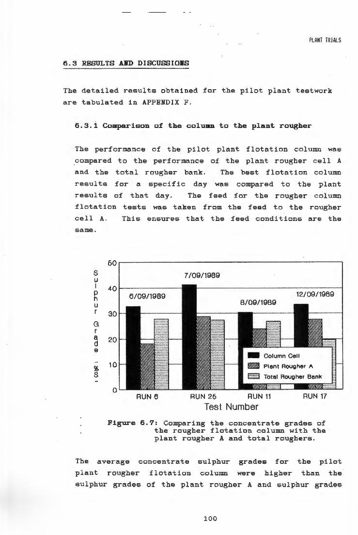
PLANT TRIALS

6.3 RESULTS AJID DISCUSSIOIS

The detailed results obtained for the pilot plant testwork

are tabulated in APPENDIX F.

6.3.1 Comparison of the coluDD. to the plant rougher

The performance of the pilot plant flotation column was

_compared to the perf"ormance of t .he plant rougher cell A

and the total rougher bank . The best flotation column

results

results

for

of

a specific day

that day. The

was compared to the plant

feed for the rougher column

flotation t .ests was taken from the feed to t .he rougher

eel 1 A. This ensures that t .he feed conditions are the

same.

s u I

~ u r

G r a d 8

% s

40 6/09/1989

30

20

0 RUN 6

7/09/1989

12/09/1989 8/09/1989

Plant Rougher A

Total Rougher Bank

·=·=·=·=·=·=·=·

RUN 26 RUN 11 RUN 17

Test Number

Figure 6.7: Comparing the concentrate grades of the rougher flotation column with the plant rougher A and total roughers.

The average concentrate sulphur grades for the pilot

plant rougher flotation column were higher than the

sulphur grades of the plant rougher A and sulphur grades

100

PLANT TR IALS

from the total plant rougher bank <Figure 6. 7). The

flotation column can thus be used as a rougher to achieve

higher concentrate sulphur grades than is possible with

conventional flotation. This is due to the cleaning of

the froth using wash water.

The average sulphur recoveries for the flotation rougher

column were also higher

calculated for the plant

than the sulphur recoveries

rougher <Figure 6 . 8) . For

run 17, on the 12/09/1989, the superficial air rate was

3,02 cm/sec which resulted in a recovery of 39% sulphur .

These improvements in recovery and grade over the plant

confirm the results obtained in laboratory results.

8 60 .------------------------, u I

~ 40

• Column Cell

a Plant Rougher A 12/00/1989

u r R 30~-~~--~~~~~~~~~~~~

e C 0 V e r y

% s

8/09/1989

10

0 RUN 6 RUN 26 RUN 11 RUN 17

Test Number

Figure 6.8: Comparing the sulphur recoveries of the rougher flotation column with the plant rougher A.

The gold recoveries of the rougher flotation column were

compared to the plant rougher and the total plant gold

recoveries <Figure 6. 9). For run 19 on the 12/09/g189,

the average gold recovery for the flotation column was

about 61% compared to the plant rougher gold recovery of

101

PLANT TRIALS

about 43% and t .he overi':tll plant. recovery of about. 61 %.

This was only possible at. superficial air flow rates

greater t.han 3, 02 cm/sec. This was probably because of

the improved floti':ttion of coarse pyrite pi':trticles (which

contain more gold) at a high superficial air rate.

The results from run 19 again show that the flot.ation

column can perform as good or bett.er than convent.ional

flotation. In this case <Run Hn t.he pilot plant column

did the work the whole plant flotation circuit did.

Figure 6.10 shows that the gold grade was similar for run

19 and for the plant on the 12/ 09/1989. For run 11 the

gold grade obtained with the column was lower t.han that

obtained by the plant. rougher and tot.al rougher ba.nk

(11/09/1989).

G 0 I d

R 9 0 0 V 6 r y

% A u

80

60

0

11/09/1989 ----·---··-·-·----------------------·-------------·----·------

RUN 16

.:.:.:.:.:.:.:.:.:.:.:.:.:.:::.: ..

12/09/1989

- Column Cell

B Plant Rougher A

f:::=:::::=::I Total Rougher Bank

~\\\\\~\\\\\\\~ RUN 19

Test Number

Figure 6. 9: Comparing t.he gold recovery of the rougher flotation column with the plant rougher A and total plant roughers.

Figure 6. 11 shows that the t.heoret.ical mean liquid

residence t.ime <Volume/ Volumetric flow rat.e) for the

pi lot plant flot.ation col 1.1mn in rougher mode was nearly

102

PLANT TR IALS

twice as long as that of t .he plant rougher . On the

7/09/1989 when the mean liquid residence time of the

G 0 I d

G r a d e

~ t 0 n

L

26

20 - -

16 ----

0

11/09/1989

RUN 16

- Column Cell

a Plant Rougher A

E:Z.1 Total Rougher Bank

~\\\\\\~~\\\\\\, ::;.; .:.:,:.;.;.;::.~:-:,:-:.;.:.

RUN 19

Test Number

Figure 6.10: Comparing the concentrate grades of the rougher flotation column with the plant rougher A and total roughers.

I 25....--~~~~~~~~~~~~~~~~~~~~--, q u I

d 20 R 8 8 I d e n 0 e

T I m

16

10

e 5

m

~ 0

• Column Cell Res Time

D Column Recovery

• Plant Res Time

t7lll/A Rougher A Reoovery

Shorter Column Residence Time

RUN 8

7/09/1989

RUN 24 RUN Q

Test Number

8 12/09/1989 u

-''- -'-40 ~

RUN 18

u r

A e 0 0

20 V e r y

% s

Figure 6.11: Comparing the mean liquid residence time of the rougher flotation column with the plant rougher A.

103

PLANT TRIALS

flotation column was less than that of the plant rougher

cell due to a high volumetric feed rate being used. The

sulphur recovery obtained with the column was still more

than that of the plant rougher.

6.3.2 Comparing the column to the plant cleaner

The pilot plant flotation column was compared to the

plant cleaner cells. For these cleaner column flotation

tests the feed for the column was taken from the feed to

the cleaner cells. A sample from the feed to the plant

cleaner was taken i:lnd pumped into the holdup t .ank.

here the pulp was pumped into the flotation column.

From

The sulphur grades obtained with the cleaner flotation

col uinn are in the ri:lnge of 15. fl% to 19. 6% compared to the

16.0% obtained with the plant cleaner <Figure 6.12). The

sulphur recoveries obtained in the flotation column Ztre

much lower though t.han the theoretical recoveries of the

plant cleaner cells. This low sulphur recovery was due

to the column operating above the maximum carrying

s u I

~ u r

G r a d 8

% s

25.--~~~~~~~~~~~~~~~~~~~~~~~75

Cleaner Column Cell Plant Cleane

16

10 30

6 6ulphur GrMes 15

• Sulphur Recoveries

0 Teat 12 Teat 13 Teat 14 Plant Cleaner

Test Number

8 u I

~ u r

R e C 0 V e r y

% s

Figure 6.12: Comparing t .he sulphur grade and recoveries between the cleaner flotation column and the plant cleaner cell .

104

PLANT iRIALS

capacity. It was visually observed that the maximum

carying capacity was reached as most of the collected

solids were washed back into the collection zone . The

feed to the column could not be reduced due to physical

limitations of the solids settling out in the feed lines

at lower feed rates.

6.3.3 Using the column in a rougher-scavenger mode.

The pi lot plant :flot.ation column was used in a rougher

scavenger mode. The feed for the flotation column was

taken from the feed to the plant rougher A. This would

determine the maxi:m1.1m sulphur recovery possible if no

additional reagents are added . In the plant flotation

circuit additional collector is added to the feed at the

2 nd middlings float and frother is added to every

flotation bank. No additional reagents were added to the

column flotation circuit.

The sulphur grade from the rougher flot.ation column was

20. 0%, and 11. 5% from the scavenger flotation column .

This resulted in a grade of 19.1% for the total

concentrate. To obtain better grades the air rate would

have to be reduced and the low grade sulphur concentrate

from the scavenger flotation column should possibly be

returned to the feed for the rougher column. The effect

of varying the superficial air rate is discussed section

6.3.5 .

The sulphur recovery in the rougher flotation column was

47% and in the scavenger column 5% <Of total sulphur feed

to plant). This resulted in a total sulphur recovery of

52% for the column operating in a rougher-scavenger mode.

This sulphur recovery is much lower than the theoretical

plant recovery <Calculated by Buffelsfontein Mine) of

65 . 6% and the actual plant sulphur recovery of 71. 7%

<Plant values are average values for 7 months up to

31/07/ 1989). The reason for this low sulphur recovery

105

PLANT TRIALS

with the flotation column setup was possibly due to less

reagents being added to the column than to the overall

flotation plant. Less reagents were added to the pilot

plant flotation column because t .he plant has additional

reagent feed points to the flotation cells.

6.3.4 Effect of varying the superficial wash water rate.

By increasing the superficial wash water rate from

0 cm/sec to 0.18 cm/sec the concentrate sulphur grade

increased from 22. 0% to 32. 8%. This improved grade was

also reported in the literature <Kosick, G.A. and

Kuehn, L., 1988i Nicol, et al., 1988 i Yncha ust i, et

al. I 1988i Parekh, et al., lf!88). The grade was

improved because entrainment is reduced with increased

wash water addition. Increasing the superficial wash

water rate above 0.18 cm/sec did not further improve the

60 60 8 s u u -G- Grade -+- Recovery I I 40 -----· 40 ~ ~ u u r r 30 ---- 30 R G e

r C 0 a 20 20 V d e e r

10 10 y

% s %

s 0 0

0 0.06 0.1 0.16 0.2 0.26 0.3

Superficial Wash Water Rate ( cm/sec)

Figure 6. 13: The effect of increasing the wash water rate on the sulphur grade and recovery for the flotation column.

106

PLANT TRiALS

grade (Figure 6 . 13), The maximum grade obt.ainat,le by

varying the wash waster rate was thus 32.8% sulphur at a

superficial wash water rate of 0.18 cm/sec or greater.

The sulphur recovery improved :from 6% to 14% as the

superficial wash water rat.e was increi:1.sed :from O cm/sec

to 0.18 cm/sec <Figure 6.13).

The sulphur recoveries were so low because high feed

rates were ·used. The col1..1mn was

maximum carrying capacity with

the :floated material dropped

thus operated above the

the result t .hat. most of

back into the collection

zone. This was observed visually.

Increasing t.he super:fi c ial wash wat.er rate

0.18 cm/sec decreased the sulphur recovery to 12%.

above

That

excess wash wat.er decreases the recovery was reported by

Kosick (1958) and Luttrell ( 1 fl58), This decrease in

sulphur recovery at high wash wat.er rates was ;:,.lso

observed in the laboratory tests.

The mass recovery re;:,.ched a maximum of 0.69% at a

superficial wash water rat.e of 0 , 18 cm/sec (Figure 6. 14) .

This t.rend in:fluenced the sulphur recovery as discussed

above. The increased wash w;:i.ter addition r;:i.te incre;:,.sed

the :froth carrying capl'tci ty due to the froth bec,oming

more st.able . The s tabilit.y prevents the b1..1bbles :from

coalescing, and t .here:fore reducing the carrying

capacity . At. excessively high w;:,.sh w;:i.ter addition r;:i.tes

collected solids are washed out. of the :frot.h. The mean

1 iquid residence t .ime ( Est.imat.ed) was also decreased

which resulted in a lower recovery.

The solids densi t .y in the concent.rat.e decre;:,.sed as t.he

superficial wash wat.er rat.e was increased. The decrease

in the E-Dl ids densi t.y o:f the concentrate was much greater

at superficii:!.l 1,,msh wat.er velocities greater than

0.18 cm/sec. This increased water recovery in the

107

PLANT TRIALS

concentrate was wat.er from t.he addi t.ional wash wat.er

added and not from the feed pulp.

These t.rends were also observed in t.est. c,arried out. with

the column operating as a cleaner (Figures 6.15 & 6.16).

M a 8 8

R e C 0 V a r y

%

1 ~~~~~~~~~~~~~~~~~~~~~--.25 8 0 I I

----··------,--.. ·---·--·-----------·--·-----.. ------·---.. ·-·-·---·--·---.. --·---·-·-- 20 d

D

X

0.4 .......... -........................... - ........ _,_ .......... ,_,_, _____________ ,, ____ , __ ,_ .......... ---------·-·-· -----·--·---·--.. -................... 1 0

0.2 .................................. - .................. _ .. __________ , ____ , _____ , __ ,, __ , ___ ,_,,,, ______ ,, ___ ,_,_, ______ ,, ____ , ________ ,,......... 5

0 .__ __ __,L.,__ __ _. ___ __._ ___ __._ ___ _..._ ___ _, 0

0 0.06 0.1 0.16 0.2 0.26 0.3

Superficial Wash Water Rate (cm/sec)

Figure 6. 14: The e:ffect. of wash water rate on the percent solids recovered and the solids percent (mass/mass) in the concentrate.

108

8

p e r C e n t a g 9

%

s u I

~ u r

G r a d 8

% s

M a 8 s

R e 0 0 V e r y

PLflNT TRIALS

. I -8- Grade -f- Recovery I 4 o -·-.Dp.t1mum .. .Rec0¥er-v. .. -·---·---·-· .. - -·· ·---·-·····-········-· ·--· -· ······-··-- 4 o

1 0 --·--··-··--··-·--··---··--··-·--------···----------·- ------·--··--·---·------··---··---··--··-·--····-·--· 1 0

O'-~~--'-~~~--'-~~~-'--~~~-'-~~~'-~~~o

0 0 .05 0 .1 0 .15 0.2 0.25 0 .3

Superficial Wash Water Rate ( cm/sec)

Figure 6.15: The effect. of increasing t.he wash water rate on the sulphur grade and recovery for the cleaner column.

-G- Grade

~ Reoovery

5 ·---··---···················-----·····-······----··-··-··--·-··-·----·-- ·-·--·---------···-----·······-·······--··----· 5

QL-~~-'-~~~---'-~~~-'-~~~...__~~~'-~~-'Q

0 0.05 0.1 0 .16 0.2 0.26 0 .3

Superficial Wash Water Rate {cm/sec)

~ u I

g u r

R e C 0 V e r y

% s

Figure 6.16: The effec t. of wash water rate on t.he percent solids recovered and the solids percent <:mass/:mass) in the column cleaner concentrate.

1 09

8 0 I I d s

p e r C e n t a g e

PLANT TRIALS

6.3.5 The effect of varying the superficial air velocity

Increasing the superficial air velocity from 1. 22 cm/ sec

to 2. 06 cm/sec decreased the concent.rat.e sulph1.1r grade

from 38 . 3% to 30.8% (Figure 6.17). This decrease in the

grade with increasing air rat.e has been shown by several

researchers C Gooda 11, C. M. zmd o·- Connor, C. T. , l 98fi;

Misra, M. and Harris, R., 1988; Parekh, et al., 1988) .

This decrease in the concentrate grade is due to

increased entrainment caused by increased air velocities.

During a subsequent test. the

increased from 3.02 cm/sec

superficial air rate

to 3.57 cm/sec.

was

The

concentrate sulphur grade decreased from 33.4% to 17.6%.

When the superficial air rate was :furt.her increased to

4.19 cm/sec, the concentrate grade improved to 20%.

The sulphur recovery reached an opt.imum of 14% at a

superficial air rat.e of 1. 86 cm/sec (Figure 6. 17). This

optimum in recovery was repeatedly reported (Dobby, D.S.

and Finch, J. A., 1986; Parekh, et. al., lf188 ;

Goodall, C.M. and o·-connor, C.T., 198fi; L1.1t.t .rell, G.H.,

1988). The optimum in t .he s1.1lphur recovery is due to the

bubbles coalesing. Initially the carying capacity

increases with an incresed air rat.e, but. when the

bubbles start t .o coalesce, the carrying capacity is

reduced and therefore the recovery starts to decrease.

When the superficial air rates were increased during a

subsequent test (from 3. 02 cm/sec to 4. 19 cm/sec), the

sulphur recovery increased from 39% to 47%. This

increase is due t.o a higher mass recovery at. a high

superficial air rate.

The percent solids recovered in the concent.rat.e at low

superficial air :flow rat.es (up to 2. 06 cm/sec) increased

up t.o a maximum of O. 67% +-0. 02% (Figure 6. 18). At high

superficial air rates <greater than 3.02 cm/sec) the

110

PLANT TRiALS

percent solids reporting to the concentrate increased

from 1.66% to 3.74% (Obtained in a subsequent test).

G r 6 d e

% 8

M a s s

R e 0 0 V e r y

4 0 -··--····---------·····-··--··-----··--··-··-----·-----·-----·---·----···-·--··--·--·---··----'--····----······----·- 4 0 R

30 --··-···--·---·--··--··-------------·---·-·--------·-------------· ---·------··-·-··----··- 30

20 ··--··-------·-------·--·-··---·-----·---·-·---·--·--·--·-·-----·-·---·- 20

± 10

--~.,.- ---+ -··----··---~ ---···-·------------------·----·--·--

' -e- Gr a.de -+- ~eoover y I 10

01.-______ _._ _______ ...._ ______ _.o

1 1.5 2 2.5

Superficial Air Rate (cm/sec)

Figure 6.1'7: The effect. of air flow rztte on the grade and the recovery for the pilot plant flotation column.

e C 0 V 9 r y

% s

1.....---------------------------,

0.8

o. 6 ··---·-·---·--·--····-··-----·------------·-

0.4

0. 2 --·---·--··--···-··---··--··---····-------·-···---·-·-·--------·--·--··--·-·-·---·-··--·-······--·-··---····-··-···-····-····--·-·-···-··-

o.__ _______ _._ ________ ....._ _______ __.

1 1.5 2

Superficial Air Rate (cm/sec)

Figure 6. 18: The effect. of air flow rate on the percent solids recovered .

111

2.5

PLANT TRIALS

The effect of increasing the superficial air flow rate

from 1. 83 cm/sec t .o 3. 60 cm/sec increased the gold

recovery from 27% to 63% <Figure 6.19) .

R e C 0 V a r y

% A

70.----------------------------, 60 --------------- ---- ·-----------

50 --------·--

40 ---·---------------

30 ------ o -----PCANT~COVERY

20 --------------- -------ROUGHER-----TOTAL u 11/09 Au 54% Au 79%

10 -------------------- --l2le9----A++U·--4-8%-----Att-6+%-

0'-------~-----------~-----~ 1 2 3 4

Superflclal Air Flow Rate ( cm/sec) Figure 6.19: The effect of air flow rate on the

total gold recovery.

112

5

PLANT TR IALS

6.4 SUDARY OF THE PLAIT TRIALS

1) The pilot plant column flotat.ion cell can be used to do

on site test work.

2) The column flotation cell was used on a pyrite flotation

circuit as a rougher cell producing improved sulphur

grades. Sulphur recoveries were however lower . The gold

recoveries and grades were similar to those of the plant.

3) The pilot plant flat.at.ion column yielded improved sulphur

recoveries at shorter residence t .i:mes than the plant

rougher cell .

4) By increasing the wash water rate the sulphur concentrate

grade can be improved.

5) By increasing the air rate the gold recovery can be

increased.

113

COICLUSIOIS

CHAPTER SEVEN

For this research on the determination of the effects of

physical and chemical paramet.ers on the flat.at.ion column cell

performance in the flot.ation of pyrite, a laboratory and a

pi lot flotation column were designed and built. Using the

flotation columns with the experiment.al procedure developed

produced highly repeatable results.

In view of the experimental test work conducted the following

conclusions can be drawn:

7.1 The flotation column produced better sulphur grades than

conventional flotation due to the flotation column~s deep,

water washed froth, reducing entrainment into the

concentrate. This was confirmed by plant test work.

7.2 The flotation columns yielded higher sulphur recoveries

than conventional flotation at lower residence times due

to the flotation columns counter-current contact mechanism

of the bubbles and the particles.

114

CONCLUSIONS

7.3 An increased air rate yielded an optimum in sulphur

recovery. The increase in recovery was due to an

increased mass pull which resulted from an increased

superficial bubble surface rate as the air rate was

increased. The optimum in sulphur recovery was due to the

superficial bubble surface rate decreasing at high air

flow rates.

7.4 The concentrate sulphur grades decreased as the air rate

was increased. This was because of increased entrainment.

7.5 Increasing the collection zone length increased the

sulphur recovery to its maximum because of an increased

solids residence time. Maximum recovery was obtained at a

4 meter collection zone length.

7 . 6 The sulphur grade decreased while the sulphur recovery

increased when the collection zone length was increased.

7 . 7 Increasing the froth depth decreased the recovery. This

decrease was due to an improved cleaning effect and froth

instability at deep froth depths.

7 . 8 The grade increased as the froth depth was increased due

to an increased cleaning action of the froth . The

cleaning action was however reduced when the froth depth

was increased too much, due to the froth collapsing at

times.

7 . 9 Increasing the feed solids percentage to the flotation

column had no effect on the grade or recovery. The

recovery did however decrease when the maximum carrying

capacity was reached .

7.10 The volumetric feed rate to the flotation column should

be high enough so that there are enough particles to

stabilise the froth . A high volumetric feed rate

115

CONCLUSIONS

therefore yielded better concentrate grades than a low

volumetric feed rate.

7.11 Increasing the volumetric feed rate resulted in operating

at the maximum carrying capacity. A further increase in

volumetric feed rate, or a too short solids residence

time, would decrease the recovery.

7.12 Increasing the wash water rate increased the concentrate

grades. This was due to an increased froth stability and

a higher washing rate. When the wash water was increased

too much, the froth became unstable,

decreased concentrate grade.

resulting in a

7.13 Lowering the wash water distributor decreased the water

recovered into the concentrate. This was due to more time

being allowed for drainage of the water.

7.14 Wash water at a high temperature increased the

concentrate grades while less water was recovered. The

wash water at a higher temperature has a lower viscosity

and therefore it drains out of the froth easily,

increasing the cleaning effect.

7 . 15 Lowering the feed position increased the grade while the

recovery decreased. This was caused by an increase in the

cleaning zone and a decrease of the collection zone.

7.16 When the flotation column was used the chemical

parameters which were varied showed the same trends as

conventional flotation. Leaching the ore and adding more

collector increased the recovery.

7.17 At low frother dosage rates the froth became unstable and

the recovery decreased. It is therefore important to

maintain a stable froth.

116

REFEREICES

ANELUNXEN, R.L., LLERENA, R., DUNSTAN, P. and HULS, B. 1988, Mechanics of Column FLotation Operation, Proceedings of an International Column Flotation Symposium, Chapter 16,p149-156.

CONTINI 1 N.J., WILSON, S.W. and DOBEY, G.S., Measurement of rate data in flotation columns., Proceedings of an International Column Flotation Symposium, Phoenix, Arizona, January 1988, Chapter 10,p81-89.

DOBBY 1 G.S. and FINCH. J.A. 1 Flotation column scale-up and modelling., CIM Bulletin;79, No. 889, May 1986,p89-96.

DOBEY, G.S., YIANATOS, J.B. and FINCH, J.A., 1988, Estimation of bubble diameter in flotation column from drift flux analysis, Canadian Metallurgical Quarterly, Vol. 27 1

No.2, p85-90.

EGAN, J.R., FAIRWEATHER, M.J. and MEEKEL, W.A., 1988, Application of column Flotation to Lead and Zinc Beneficiation at Cominco, Proceedings of an International Column Flotation Symposium, Chapter 4, p19-26.

ESPINOSA-GOMEZ, R., YIANATOS 1 J. 1 FINCH, J and JOHNSON, N.W., Carrying capacity limitations in flotation columns., Proceedings of an International Column Flotation Symposium, Phoenix, Arizona, January 1988, Chapter 15, p143-148.

FEELEY, C.D., LANDOLT, C.A. 1 MISZCZAK 1 J. and STEENBURGH 1

W.M., Column flotation at INCO's matte separation plant, 89th annual general meeting of CIM, Toronto, May 1987.

FINCH. J.A. and DOBEY, G.S., Column flotation. 1 Column flotation course, Camborne School of Mines, Cornwall 1

England, April 1988.

FOOT 1 D.G., Jr, McKAY 1 J.D. and HUIATT, J.L., Column flotation of chromite and fluorite ores. 1 Canadian Metallurgical Quarterly 1 Vol. 25, No.1 1 p15-21 1 1986.

GOODALL, C.M. and O'CONNOR, C.T., Residence time distribution studies of the solid and liquid phases in a laboratory column flotation cell., Proceedings of an international column flotation colloquium, Gordon's Bay, South Africa, August 1989, Volume 2.

117

GOODALL, C.M. and o~CONNOR, C.T. 1991, Residence time distribution studies in a flotation column. Part 2: The effect of flotation variables on the residence time distribution of the solids and liquid. Int. J. Min. Proc, Submitted for publication (1991).

HU, W. and LIU 1 G., 1988, Design and Operating Experiences with Flotation Columns in China, Proceedings of an International Column Flotation Symposium, Chapter 6.

KOSICK, G.A., FREBERG, M. and KUEHN, L., 1988, Column flotation of galena at the Polaris Concentrator., CIM Bulletin, Vol. 8 1 No 920, p54-60.

LUTTRELL, G.H., WEBER, A.T., ADEL 1 G.T. and YOON, R.H., 1988, Micro-bubble FLotation of Fine Coal., Proceedings of an International Column Flotation Symposium, Chapter 21.

MISRA, M. and HARRIS, R., Column flotation of fine coal from waste coal refuse., Proceedings of an International Column Flotation Symposium, Phoenix, Arizona, January 1988, Chapter 25.

NICOL, S.K., ROBERTS, T., BENSLEY, C.N., KIDD, G.W. and LAMB, R., 1988, Column Flotation of Ultrafine Coal -Experience at BHP-Utah Coal Limited~s Riverside Mine, Proceedings of an International Column Flotation Symposium, Phoenix, Arizona, p7-11.

O~CONNOR, C.T., DUNNE, R.C. and BOTELHO DE SOUSA, A.M.R., 1984, The effect of Temperature on the Flotation of Pyrite, Journal of the South African Institute of Mining and Metallurgy. ,volume 84, Number 12, pp 389-394.

PAREKH, B.K., GROPPO, J.G., STOTTS, W.F. and BLAND, A.E., Recovery of fine coal from preparation plant refuse using column flotation., Proceedings of an International Column Flotation Symposium, Phoenix, Arizona, January 1988, Chapter 24.

REDDY, P.S.R., PRAKASH, S., BHATTACHARYA, K.K., SASTRI, S.R.S., and NARASIMHAN, K.8., 1988, Flotation Column for the Recovery of Coal Fines., Proceedings of an International Column Flotation Symposium, Chapter 23.

SUBRAMANIAN, K.N., CONNELLY, D.E.G. and WONG, K.Y., Commercialization of a column flotation circuit for gold sulphide ore., Proceedings of an International Column Flotation Symposium, Phoenix, Arizona, Chapter 3, p13-18.

WHEELER, D.A., Historical view of column flotation developement., Proceedings of an International Column Flotation Symposium, Phoenix, Arizona, Chapter 1, p3-4.

118

YIANATOS, J.B., A review of column flotation modelling and technology., Mineral Processing Report, Department of mining and metalurgical engineering, University of Queensland 1 June 1987.

YIANATOS, J.B. 1 FINCH, J.A., DOBBY, G.S. and LAPLANTE 1 A.R., Effect of column height on flotation column perfor1nance 1

Minerals and metallurgical Proc., 4(1), 11-14.

YIANATOS, J.B., FINCH 1 J.A. and LAPLANTE, A.R., The cleaning action in column flotation froths., Transactions 1 The institution of mining and metallurgy, (Section C) 1 1987, 96, 199-205.

YIANATOS, J.B., FINCH, J.A. and LAPLANTE, A.R., 1988 b, Selectivity in column flotation froths, International Journal of Mineral Processing 1 15 1 p279-292.

YNCHAUSTI, R.A., McKAY, J.D. and FOOT, D.G. Jr., 1988, Column Flotation Parameters - Their Effects, Proceedings of an International Column Flotation Symposium, Chapter 17.

119

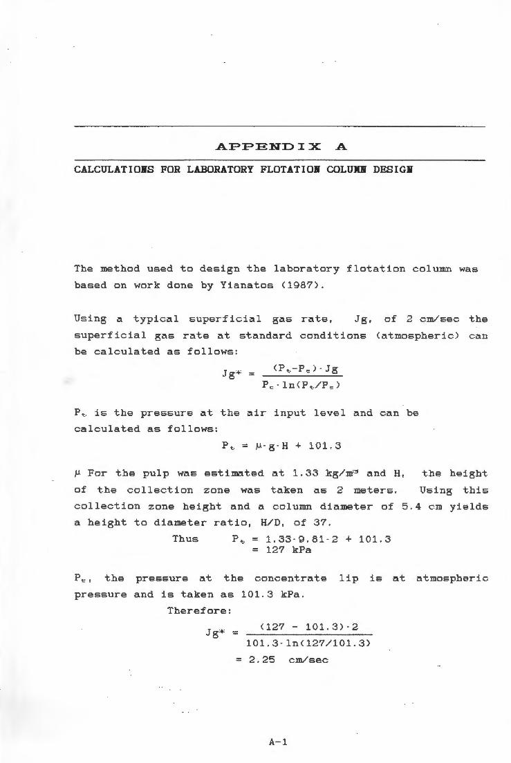
APPENDIX A

CALCULATIONS FOR LABORATORY FLOTATION COLUJIJl DESIGN

The method used to design the laboratory flotation column was

based on work done by Yianatos (1987).

Using a typical superficial gas rat.e, Jg, of 2 cm/ sec the

superficial gas rate at standard conditions (atmospheric ) can

be calculated as follows:

Jg:.;.: = ( p "· - p '= ) - Jg

P c - ln<Pt./P-= )

P ~ is the pressure at the air input level and c an be

calculated as follows:

P~ = µ - g - H + 101 . 3

JJ. For the pulp was estimated at. 1. 33 kg/m'3 and H,

of the collection zone was t .aken as 2 meters.

the height

Using this

collection zone height and a column diameter of 5 . 4 cm yields

a height to diameter ratio, H/D, of 37.

Thus p~ = 1 . 33-9 . 81-2 + 101 . 3 = 127 kPa

P"', t .he pressure at the concentrate lip is at atmospheric

pressure and is taken as 101.3 kPa.

There:fore:

Jg=+: = (127 - 101. 3) - 2

101.3 - ln(127/101.3)

= 2.25 cm/sec

A-1

APPENDIX A

The bubble diamet.er, d i::, , was estimat.ed as 0 . 2 cm. The bubble

diameter at the t .op of the froth, d 1::, :+:,

assuming a 50% increase in bubble diameter:

is est.imated by

Now the

c alculated.

superficial

di:,,:+: = 2-d!:,o = 2 - 0.2 = 0. 4 cm

bubble surface

Js = 6 - Jg:+:

d1;:,:.i:

= 6 - 2.25

0.4

rat.e, Js, can be

The 80% passing particle size, d ~,:, , was est.imated to be about

50 microns.

Using the following equation to bias the smaller particles:

d i=' = 0 ·. 3 · d ~ 0

= 0.3 - 50 = 0 . 0015 cm

Assuming that each particle is spherical and occupies d p 2 of

the bubble surface, then the bubble surface required per gram

of solids is:

Sr= 6

= Pi-15-2 . 23

= 571 cm:.: /g

Assuming that each particle is shared by two bubbles at the

overflow, t .he effective superficial bubble surface rat.e, Jse

is :

Jse = 0 . 5 - Js = 17 cm2 /s/cm·~

The superficial floated particle rate, Jpf, is therefore given

by:

Jpf = 3600 - Jse

Sr

A-2

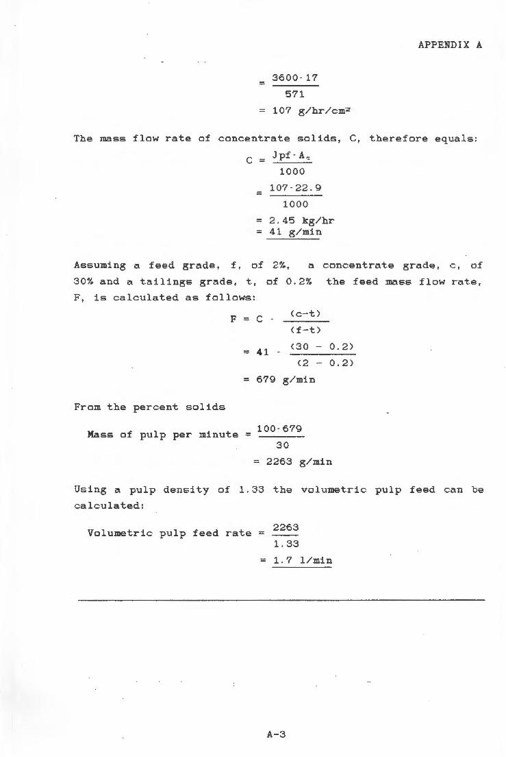
= 3600-17

571

= 107 g/hr/cm:.?

APPENDIX A

The mass flow rate of concentrate solids, C, therefore equals:

C = Jpf - A-=

1000

107 - 22.9 =

1000

= 2.45 kg/hr = 41 g/min

Assuming a feed grade, f, of 2%, a concentrate grade, c, of

30% and a tailings grade, t, of 0.2% the feed :mass flow rate,

F, is calculated as follows:

From the percent solids

F = C - <c-t)

(f-t)

= 41 -(30 - 0.2)

(2 - 0.2)

= 679 g/min

Mass of pulp per minute= 100-679

30

= 2263 g/min

Using a pulp densi t.y of 1, 33 the volumetric pulp feed can be

calculated:

Volumetric pulp feed rate= 2263

1. 33

= 1.7 1/min

A-3

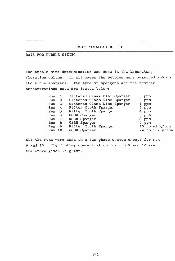
APPENDIX B

DATA FOR BUBBLE SIZIRG

The bubble size determination was done in the laboratory

flotation column . In all cases the bubbles were measured 200 cm

above the spargers. The type of spargers and the f r other

concentrations used are listed below:

Run 1: Sintered Glass Disc Sparger 0 ppm Run 2: Sintered Glass Disc Sparger 2 ppm Run 3: Sintered Glass Disc Sparger 4 ppm Run 4: Filter Cloth Sparger 0 ppm Run 5: Filter Cloth Sparger 4 ppm Run 6: USBM Sparger 0 ppm Run 7: USBM Sparger 2 ppm Run 8: USBM Sparger 4 ppm Run 9: Filter Cloth Sparger 40 to 41 g/ton Run 10: USBM Sparger 74 to 107 g/ton

All the runs were done in a two phase system except for run

9 and 10. The frother concentration for run 9 and 10 are

therefore given in g/ton.

B-1

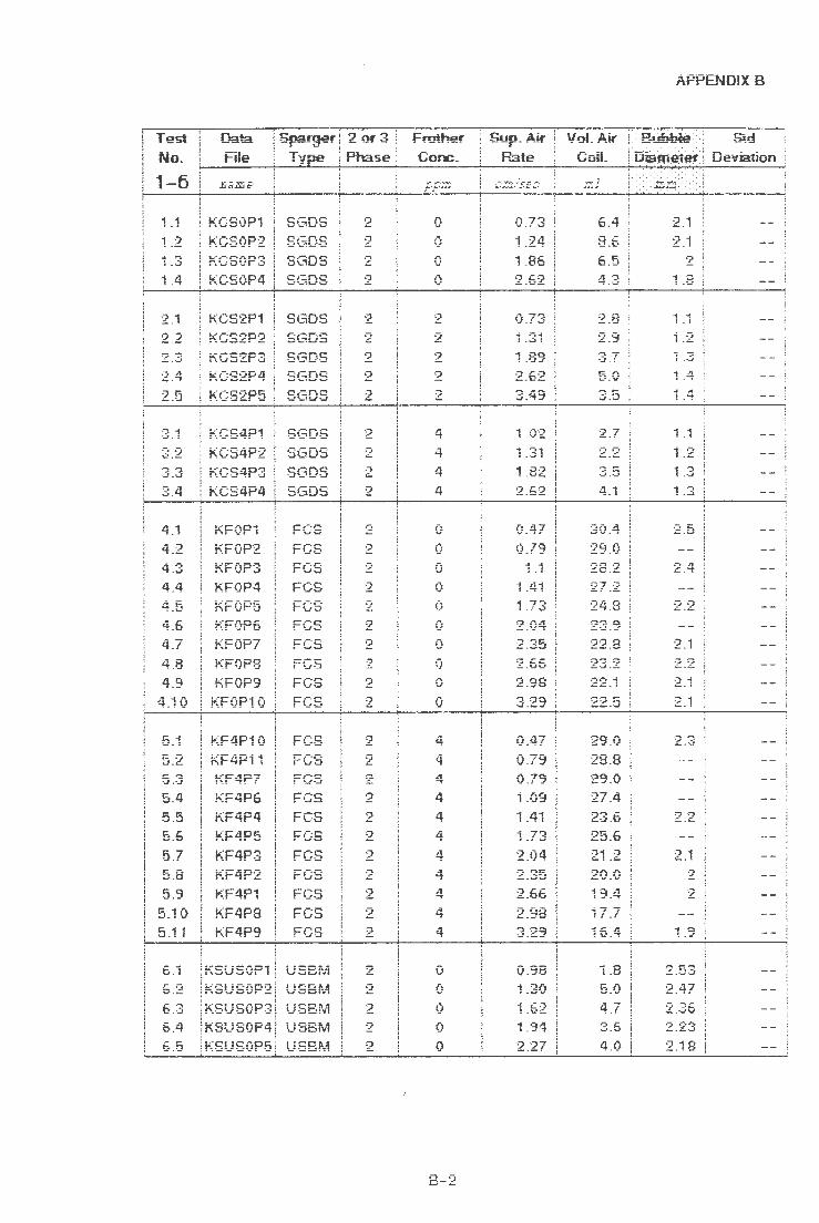
Test No.

1-6

1 .1

1 .2

-1 11 ! -~

2 .2

.-. JI .c:.-.

2 .5

3.1

3 .2 ':> ':> .....! . •J

4 .1

4.3 4 .4 4.5 4 .6

Data

File

!-=~GS0P1

KGS0P2 ?(CS0P3 !{GS0P4

i{GS2P1

?i:CS2P2

KGS2P3

i-~<:;S2P5

KCS4P2 :...-· .--c ... 10":\ ! ~.V·...l '""'!! •.J

KCS4P4

i'~FOP1

KFOP2 ;.,..· :-- .. -.. ~~ ~r·Jr.:,

KFOP4 i{FOP5

4 .7 !..:FOP?

!f .u KFOP8 4;:, i":FOP9

4.10 iffOP10

5 .1 !{F4P10

5.2 c:. ":!. ·..l . ·J

5.4

5 .5 5.6

5.7 !:, .8

5 .9

5 .10 "' .... • ... L! I

5 .1

6 .2 6 .3 6.4

6 .5

iS:F4Pi 1 1..-·c ... .,--7 !'.I :r1

KF4P6 KF4P4

KF4P3 :~· ;--r.r..-. r,r"'tr.c:

KF4P1

KF4P8 KF4P9

KSUSOP1 KS•JS0P2

KSUS0P3

KS!JS0P5

E-par-ger 2 ~ ... 3

Type Phase

SGDS SGDS SGDS

SGDS

SGDS

SGDS SGDS S(3DS SGDS

FCS FGS FCS FGS FCS c.--c ! ~.J~

FCS f V--1

FCS FGS

FGS

F(}S

FCS FGS

FGS FCS FGS FGS c,--c ! 'foJ-~

lJSBfvi US8~.;1

US8M USBtv1

IJSBM

2

2 2 2

2

2

2

2

2 2 2 2

2

2

2

2

2 2 2 2 2 2

2

2 2 2

2

F r.::rther

Cone.

0

0 0 0

2 2

2 2

4

4

4 4

0

0 0 0 0

0 0

0

0

0

4

4 ,, .,. 4

4 4

4 4 4

4 4

0

0

0 0

0

8-2

Sup. Air Rate

. -- -7:-:-.:' c..::. ... - .

0 .73

1.24 1 .86

2 .62

0 .73 1.31

1.89

3.49

i .31 1 .82 2.62

0.47

0.79 i .1

1 .41 ; I-""'., I .f ~

2.04 2.35 2 .65 2.98

3.29

0.47

0 .79 O.?~ i .09

1 .41 ~ 7:-, ; _; ~

2.t')4 .-. :-.r: L.~~

2.66

2 .98 3.29

0 .98

1 .62

2 .27

Vot Air

Cull.

r ..:1 c.~

8.6 6 .5

4 .3

2.8

2.9

3 .7

5.0

2.7

2.2

4 .1

30 .4 29.0 28.2 27.2 24 .8 23 .9 22 .8 !'J-:, '!"j: ::...•.J • .::...

22.1

22.5

29 .0

28 .8 29 .0 27 .4

25 .6

21 .2 20.0 19.4

17.7 16.4

1 .8

5.0

4.7 3 .6

4 .0

APPENDIX B

.........

Piiim~1~ De•1iation

: . : . : : ~j;:i~ :: ::: .

2.1 :~ i

2 1.8

.... I. I

i .2

1.4

1 .4

1 .1 1 •:) ~ ':> l .·J

i .3

2.5

2 .4

2 .2

2.i

2.2 2 .1

2.1

2.3

2 .1 2 2

.. <> ! . .J

2 .47 2 .:36 ;-. ..-.. -.. L.L..:i

Test

No_

7-iO

7 -j : .:

7.2 7? ! . -..J

7 .4 7 :; ! .•J

0 "i '..!.!

8 .:?

8 .3

8.4

Ci ., _ .. _ !

9 .2 0 ·:i .J .-~

9 .5

07 J .!

9 .8

3.3

9 .1 1

9 .13

9.i 4 0 -,,:: ..!.l ·J

9.i 6

9.17

9 .18

10.1 10.2 10.3 10.4 10.5

10.6 10.7

10.8 10.9

10.10

iO .ii 10.12 i 0 .13

Da~ File

113111f'

!{SUS2P1

KSiJS2P2 !."Cl !CC'.)0? ! ".·J 1.J ,J,:_1 ·..J

l-:SUS:2P4

1\:::, l.}!:;;;'.t"'5

i<SUS4P1

KS!JS4P3 i.-· r -i ir-.:io,."i f"',O",.J0"1r"1

;{SUS4P5

rl r2

r3 r4

r5

-7 f!

r8

r11 ri 2 r13

ri 4 r15

r •. 9 ·~ tr3

rr3 n-4 rr5 rr6

rr7 rr8

rr9 rri 0

n-12 rr13 rr14

Spa~'° 2or-3 Type Phase

US8t111 tJSBl\:1 US8ti.r1

US8fvi

US8iv1 I ; ,.-.r;,a, 4 'J~D:Vi

US8fv1

US8rv1

FCS FGS FGS FGS FGS FCS FGS

FGS FC.:S FGS r-,-. r. r•w=>

FGS

FGS FCS FCS FGS FCS

US8M

!JSBM US8M

USBM

USBi',;i

USBt.4

US8iv1 tJSBtvi !JS8M

USBM

US811.'1

2

:2

2

2 2 2

? . .,

3 3

3 .:; ..... .:)

3 3 3

3 ? .., 3

3 3

3 3

3 3 ? . ., 3

3 3

3

Fmthe!'"

Gone.

ppm

2

2

:2

2

4 4 4

4 4

42 42 42 41 41 4i

42

40 40 40 42 42

41

4i d-f

• I

107 107

107 106 i06

106 101

101 101 101

74 7JI ! "'"'!'

74

B-3

Sup.Air

Rate

0.98

i.30

i .94

2.27

0.98 1.30

i.94 2.27

0.88 0 .88

0 .88 1.06 1 .06

i .06

i .31 1 .31

1.52 1.52 1.52 1.74 1.74 1 .74 2.25

2 .25 2 .25

0.60

0.60 1 .10 i .i 0

1 .10

~ c~ I .;JI

1 .51

.-.. -.~ ~ . .:).:)

VoL Air

Goll.

1.50

0 .80

0.90

0 .70

0.50 CJ.60 0 .85

0 .75 0.55

4 .3 0 .7

17.8 4 ~ 4 : : • I

18.4

i5.6

i9 .6

19.2 .. Q ... : ..... t

22.1 21 .4 21 .0 2; :3 ;;~"".) --:,: ::...::...-..!

22.7

24.0

21.4 2; .0

17 .2 15.9

15.2 10.0

1.7 -, r. f .0

10.8

~ 0 r 1 .J .0

19.1

APPENDi:X B

..... .. . : ~uh~: S;d

Ci~~~: Deviation

1 _i)

i .1 "i .. I. !

i .1

1 .2

1 .2

1 .4 ... -. I. ~

"i C'.) ! . .:...

2 .12

2.04 2.'J4 1.96

2.08 2.08 2 .07

2 .13 2.14 1.95

9 .. .~- l o

:2 .1 8

2.16

2.i 7 2 .04 i .99

1.96 1.66

1.77 1.72 1 .75 2.Jj] 1 .99 2.01

0.55 0 .60

0.58 0.53 0.58 0 .59 0.64 0 .63

0.64 0.67 0 .65 0 .66 0.66

0.67

0.6'3 0.69

0.066 0.063 r. r . ::;":\ \l. '.S-.2 -..J

0 .054

0.053 0.050 0.045 0.050 0 .055

0.078 0 .071 0.073

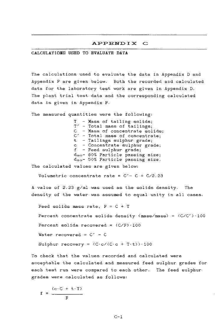
APPENDIX C

CALCULATIONS USED TO EVALUATE DATA

The calculations used to evaluate the data in Appendix D and

Appendix Fare given below. Both the recorded and calculated

data for the laboratory test work are given in Appendix D.

The plant trial test data and the corresponding calculated

data is given in Appendix F.

The measured quantities were the following:

T - Mass of tailing solidsj T' Total mass of tailings; C Mass of concentrate solidsj C' Total mass of concentratej t Tailings sulphur gradej c Concentrate sulphur gradej f Feed sulphur gradei d ~o- 50% Particle passing size; deo- 50% Parti c le passing size .

The calculated values are given below:

Volumetric concentrate rate= C'- C + C/2.23

A value of 2.23 g/ml was used as the solids density . The

density of the water was assumed to equal unity in all cases.

Feed solids mass rate, F = C + T

Percent concentrate solids density (mass/mass)= (C/C') - 100

Percent solids recovered= (C/F) - 100

Water recovered= C' - C

Sulphur recovery= <C-c/(C - c + T - t)) - 100

To check that the values recorded and calculated were

acceptable the calculated and measured feed sulphur grades for

each test run were compared to each other. The feed sulphur

grades were calculated as follows:

<c-C + t-T) f =

F

C-1

APPENDIX C/

To calculate the maximum carrying capacity the bubble size was

estimated from bubble sizing done using the spargers in a

2 phase system. The bubble sizing for laboratory test runs 12

and 13 were done during the test runs and are thus exact

values.

6 - Volumetric Air Rate Bubble surface rate, Js =

<Bubble size - 60)

60-k-3.14-d~o· (1/10000)-2.23-Jg(actual)-22.9-60 C = ...

<Bubble size - 1000)

The liquid and solids residence time was calculated as

follows:

<P-1:. - Pc)-133.23 K.;, = 1 -

9.81-H- (T'/ Volumetric tails rate)

1' 1 = 22.9-H- <l-E,..1)/(Volumetric tails rate)

u = p

1' p =

18-µ- (1+0.15-Re ... o.ee?)

(Volumetric tails rate/1374)·1' 1

<Volumetric tails rate/1374) + u ...

,. ... for t .he froth zone was estimated by assuming that the

particles collected in the concentrate have the same residence

time as the air in the froth. Therefore:

22.9-Froth Depth- <Air rate/(Air rate+ Cone. rate)) 1' ·f' r •::,,-1:-h =

Air rate

It should be noted that the above equation will not give the

exact solids residence time in the froth, but was only used

to get a rough estimate.

C-2

APPENDIX D

LABORATORY DATA

The data recorded for the laboratory test work together with

the calculated data is given in this appendix. The run number

and the parameter varied or t~ type of test done is listed

below:

Run Bo. Variable Page

1. St.ei:tdy St.i:t t.e Det.ermini:tt.ion 2. St.ei:tdy St.i:\t.e Deter mi ni:t t. ion D2-D6 3. St.e.<i:tdy St.i:tt.e.< ( 0 - ;3(1 minut.e-e. ) 4 . .St.ei:tdy St.i:t t.e (0 - 30 mi nut.es)

5. St.ei:tdy St.;:tt.e,. 05 - 2;;:: mi nut.es) 6. Wi:te.h \fot.er Temperi:t t . ure 7. Tii:\5h Wi:tt.er Te:rnperi:\t.ure 8. Reproducibility D7-D11 9. Re-produci bi 1 i t .y 10. Volumetric Feed Rat.e 11. Superficii:tl Air Ri:tt.e, sr,r,s

12. Superfi ,:::ii:tl Air Rat.e, FCS 13. .Superficii:tl Air Rat.e, USBM 14. Collect.ion Zone Height. 15. Frot.h Depth Dlc'.-D16 16. Feed Solids Dene.i t .y 17. Wi:tsh Wat.er Ri:tt.e 18. Wi:tsh Wi:tt.er Posit.ion

19 . Feed Point 20. pH 5 i:tnd 3,5 D17-D21 21. Collect.or Dosi:tge 22. Frat.her Dosage

D-1

Run No_

1-..:i

1 .1

1 .2

1 .4 1.5 1 .6 ; 7 I .f

-IC I . U

1.9

1 .10 .. 1 .. ; •• J

2.1

2.4 2.5

2.7

2.8 2.9 2 .1 0 2.i i 2.12 2 .13

2.14

2 .15 2.16 .-.. -'7 £... I I

3 .1

3 ~. -~ 3.4

3.6

4 .1 G -:;

4.4

4.5 4 .6

So:3.raer ! CoiL ! Fro1h ! Feed !-'t I ·-' j \ i Type i Height i Hei9ht Wrom Top

SGDS SGDS SGDS SGOS SGDS SGDS SGDS c,::r.c -...1'-~U ·.J

SGDS

SGDS

SGDS SGDS SGDS

SGOS SGDS SGDS S(3DS SGDS S<3DS

SGDS S{3DS

SGDS SGDS SGDS SGDS

SGOS c,-·r.c ._,,,.::1:L}-....1

SGDS SG.05 SGDS SGDS

SGOS i ~ i SGDS

SGDS SGDS SBDS

i

200

200 200

200 200

200

200

'200

200

205 205 CJ".!:. .::..'.J ·...!

205 205 205 205

205 2()5 205 205

205 205 205 205

300 300 300 300

300

300 300 300 300

300 300

iOO 100

100

100 100

100

100 100 100

100 100

50 50 5()

50 50 50 50

50 50 50 50 50 50 50 50

iOO 100 100 100 100

100

100 iOO 100 100

100 100

- -:=:--":•

110

11 0

1 i 0 11 0 110

110 i10 110 110

110 110

55 55 55

55 55 55 55 55 55 55

55 55 55

55

ii 0

110 i iO

110 110

110

110

110 -1 ~ I\ l !V

110

110 110

\ju!.

Rate

946

943 943

942 941 942 941 941 941

941 942

i 121 1162

i 105 1099

1097

1011 1240

1176 1035

1 i 71 1114 1193

1065 1150 1154 1 i G?

952 ~ r.•"'3ry. t'../..::...J

i026

977 1 r11 a:.

1025

1086

1050 1041 1096

1073 1032

D-2

Arrl::NUIX u

Ai-'rl::NU!X LJ

: \: i=:e~o:ctfr~ofttoNs>< . . . . . . .

~.-.ii.-clc ! Sr.ijric ! f ...,;;·-=, dU'

:-. ;,::i-,fl ! -u~pr 1··., jr.;; ,:,-:=i r I '["1,-1· ..-. - ! -.lJ '-1 !fYt __ :,.u --

117.f

ii 7.3

117.4

..; -I-; ,-1 If .0

117.9

1 i 8.0 11 ?.8 1 i7 .9

117.8 118.2

"'~ ~ r,. I I/ .-:J

118.1

i i2.5 112.6 111 .:2 108.6 122.5

117.5 i 06.6 123.2

118.0 115 .1 119.0 112 .1 116.5 115.9 .& ~ A A I l ., ."t

66 .5 105.1 104.3

96 .7 1 {\" ':; U'~--

103. 4

85.4

i 03.5 105.0 108.6 108.0 104.9

i 1.6

11 .6 1 1 7 t • • •

11 .7 ~ .. '7 I I . I

-11 7 : ~ - :

ii .7

i 1 .7 . . ' t I .1

11.7

9 .9 9.6

'3.6 "'..,. J.!

9.6

10.1

9 .7 9 .5

9.5

9 .5

10.0

9 .6 9.5 9 .5

6.7 9.7 9.6 9 .4

9 .6

9 .6

7 .5 9 _3 9.6 9.4

9 .5

'2 .04

2.04

2.04

2.04 2.04 2.04

2 .04 2.04 2 .04

2.04 2 .04

2 .02

2 .fr2 2.02

2.02 2.02

2.02 2_:J2

2.02 2.02 ~""l .... _."") .::...'J;;..

2 .02

2.02 2 .02 2.02 2.02

i .42 1 .42 1.42

1.42

1.42

1.83 ... ~-.--. :.c~ ... 0':l i . •-1 ·..J

.1.83

1 .83

Cat: .

2 .04

2.04 2 .04

2.03 2.04 2 .04

2.03

'2 .04

2 .03 2 .03

2 .11 1 .97

2 .28

2.11

2.47 1 .96

2.08 2.i 8

2.3:3 2.29

2.08

2.12 2 .07 2.18 :2 .i 9

3.03 -, c.r. ! _._,,.

i .63

1 .84 2.1) 1

1.52

2.05 -i ,-;.:: I .O;J

i .87

1.94 1 .91

APPENDIX D APPENDIX D

~::::::::::::::::::::::::::::::::::::::::::::::::::::~G~T:~QDI#;IH~::::::::::::::::::::::::::::::::::::::::::::::::::::::::::::::: Run No.! Collector jCol!. one I Col!ector ICo!I . two ! Cond. !Frother Tota!

I one ! Dosaqe I two I Dosaqe I Time I Type I Frother

1--4 I .fiiil1iE- g/tc.n· .r,;;me I g/tc."fi m11I Name I ppm ( w:d)

i .1 1 .2 1 .., .. .:)

1.4 1.5 1 .6 i .7 1 .8 i .9

1.10 1 .11

2.1 2 .2

2.3 2.4 2.5

2 .6 2.7 2 .8 2 .9 2 .10 2 .i 1

2.13

2 .14 2.15

2.16 2.17

3 .2 3.3

3.4 3 .5 3 .6

4 .1 4.2 ,, .0:, ,. _,._J

4 .4 4.5 4 .6

I i j Senkol 50 j j Seniml 50 j 1 ,.,. _n~·--1 i:;o ! ! .:>t::', , U ._I •

! Senkol 50 I l Senj,:oi 50

II Senkol 50 i Senkol 50 i

i C . • j .

1

...,enkoi 50 I Senl,:ol 50 j

j Senh:ol 50 ! I Senko! 50

SIBX S!BX

SIBX S!BX SlBX

SiBX S!BX SIBX SiBX SIBX

SiBX S!BX SIBX SiBX S!BX

SiBX

I i

I Senko! 50 I I~ . . cft I

:;:;enr:oi =::.iu ! j :en~m: 50 j j ,.,em~m 50 ! I Senko! 50 j j Senkoi 50 i I I cankol i.:.n t ~- t. . '\,,,:-,,:

I Senkoi 50 Senkoi50 ! Sen!-:ol 50 i Sen~mi 50 ! s-.-.•--1 t=;{\ i::- ... r,u ~v

25 25 25 25 25 25 25 25 25 25 25

17 I AFLT 208 1

17 1 AFLT 208 1 17 AFLT 208

17 1! AFLT 208 j 17 AFLT 208 I

17 1 AFLT 208 1 17 j AFL T 208 I 17 I AFLT 208 11 I AFLT 2oa I 17 j AFLT 208 1 17 i AFLT 208 I

17 1 AFLT 208 1 17 ! AFLT 208 , 17 I AFLT 208 j 17 I AFLT 208 I

17 I AFLT 200 I 17 I AFLT 208

90 90 90 90 90 90

90 90 90 90 90 90

D- 3

32 32

32 --:,::, '·""· 32 32 32 32 32 .0:,<") •..fG.

32

32 32 32

20 1 20 I 20 I :?O I - I 20 j 20 I

I!

20

20 I 20 ! 20 I 20

20 20 20 20 20

20 20 20 20 20

20 20 20 20 20 20 20

20 I 20 I 20 I

20 I 20 .!I

20

20

20 20 20 20 20

DF 200

DF200 DF 200 OF 200 DF 200 DF 200 OF 200

DF200 DF 200

OF 200 DF 200

AF 65 AF65 AF 65 AF 65 AF 65

AF65 AF 65 AF 65 AF 65 AF 65 AF 65 AF65 AF 65

AF 65 AF 65

AF65 AF 65

DF 200 DF200 DF 200

OF 200 DF 200

OF 200

OF 200

DF 200 DF200 OF 200

DF200 DF 200

22.8 22.8 22.8 22 .9 22.9 22.9

23.0 23.0 23.0

23.0

22.6 22.? 22.5 23.8 21.9

22.2 22.9 22.3 22.4

22.1 23 .4 22.5 22.3 22.i

1 9 .... ~ .o

18.8 18.6 18.2 18.6 18.5

14.4 18.i 18.5 18.2

18.5 18.6

Run No_

1-4

i .1

1.2 1 .3

1.4 1 .5 1 .6

i .7 -, C

! .•J

1.10 i ""! .. •.•I

2 .i ' ~ Q .:.. . .:::..

.-, il ~-""T

2.5

2 .6

2.8 2 .9 2.10 2 .1 i

2 .13

2.14 2 .15 2 .16 2.17

3.i

3.3

3.4 3.5 3.6

4.1 4 .2

4.4

4.5 4 .6

Rate ! Froth.er •T.:.mn ;poc 1~ 10•1 : Vo!. I i - •• , i o#OH • j i Addition !fOffi TOIJj Rate

140

140 140

140 140 140 140 140 140

140 140

200 200 200 200 200 200 200 200 200 i 200 i

i 200 i 200 ! ! 200 !

i 200 i

l 200 · ! 200 I 200 i I 140 i

! 140 i 140 i

140 I 140 !

! 140 !

140 140 140 140

140 140

20 20 20

.-... -.. LU

20 ~iJ

20 20 20 20

20 20 20 20 20 20 20 20 20 20 20 20 20 20 20

20

20

20

20 20

20

20 20 20 20

20 20

21

21 21

21 21 21 2i 21 21

21 21

21 21 2i 21 21

21 21 21 :21 21

21 21

21 21

21 21

2i 21 21

21 •:I"' ~, 21

21 21 21 21

21

5 1630

5 1630 5 1 C. ~,{\

•~~v

5 1630 C ~ ,r:-".,-.. ;J I o.:.;•J

5 1630 ,:: i630 ;J

5 1630 5 1630

5 1630 r.: 1630 ;J

5 4250 5 4250 5 4250 5 4250 5 4250 5 4250 5 4 •:it=.{\

5 4250 5 4250 5 4250 5 4250 5 4250 5 4250

5 4250 5 4•::iF.f\

~~v

5 4250 5 4250

5 i630 5 ~ :::.~r.

I \.l•..l'J

5 1630

5 1630 5 1r~{\ o ~v

5 1630

5 1630 5 i630 ~ 1530 ._,

5 1630

5 1630 5 1630

D-4

Press Top

2 .0 2 .0 2 .0

2.0 2 _()

2 .0 2 .0 2.0 2 .0

.:.. .,.:·

2 .0

0.8 0.8 0.8 0 .8 0 .8

0.8

0 .8

0 .8 0 .8 0 .8 0 .8 0 .8 0.8

0.8 0_8

0 .8

2.0 2.0 2 .0

2.0 2 .0

2.0

2 .0

2.0 2 .0 2 .0 2 .0 2 .0

Press Bott

13.:3 13.3 ; "='? ! •J. ·-·

13.3 ~,:, ,:, I -...J .·-1

... . -. ..-, '.:> • .:>

i . .J . -.J

i 3.2 13.2 i 3.2

13.2

13.2 13.2 13.2 .. r-• • , 1.:, . ..::

! 3.2

i 3.2

13.2 1 ~ •::i

13.2

.. r;, :-. J.:,.~

~,:,,:, f ._, .-.J

1'"' ,., .:> • .:>

"1? ':> • ,J _ ._,

13.3

13.3

"1':> ':> t ·~.-...:

1 ~. ,., .:, _~

~,:, ,:, I .J .·J

.. .-. r;, I .:, • .:)

13.3 1 ~ ......

..:>.~

a* -· C,O --.JI t

i .1 9

1 . ! ~ i ~ .-.

I .J ':J

1.19 i Jr.

. I ~

1 .19 1 .i ':/ 1 .19 1.19

1 .19 1.19

3.09

3 .09 3.09 3 .09 3.09

3 .09

:3 .09 3 .03 3.09

3.09 3.09

3 .09

3 .09

3 .09 3.(t3

1.19 1 ~"' . I J

1.19

1 .1 9 1.19

1 .19

1 .19 i .19 ~ ~"' I ., ., 1 .1 9 1 .19 1.19

Ari-'!:::.Ni.Ji.X. D Ari-'!:::.NUiX D

Actuai

0 .84

0 .84

0 .84 0.84 0 .84

0 .84

0.84

0 .84

0 .84

0 .84

2.2i 2.21 2.21

2 .21

2.21 '2.21 2.21 2.21 2 .21 2 .2 i 2 .21 2.21 " ""1 .::...::..1

2 .21

2 .21 2 .21

0 .84 0.84 0.84

0.84 0 .84

0 .84

0 .84

0 .84 0.84 0.84

0.84 0 .84

Sup.

8 1as

0 .08

0 .09 0 .09

0.09 0.09

0.09 0.09 0 .09 0 .09

0 .09 0 .09

0 .10

0.11 O.i 1 0 .10 O.iO

0.10 0 .11 0 .11

0 .12 0 .11 O. i i 0.12 O.i 2

0 .12 0 .12

0.12 0 .12

-0 .02 0 .08

0 .07

0 .08 0 .07

0 .08

-0 .04 -0 .02

0 .01 0 f " ::l . 'J-

0.02

0 .02

. . . ... .. .... . .. . .... .. ............. . . . >>> ~"N{;Efff.:P,.AT~:: :>:

APPENDIX D Ari-'l:::NUIX iJ

. . . . . . . . . . .

: :/ rtiu1'4G$< Run No. Vol. fvfass ! Solids CY,~ Sol. V..i-:atl:!r ::i S Vol. t..'1ass S

i-4

1 . i 1 9

1 .3

1 .4 ~ :: I • .J

1 .6 i .7 1 .8 1 .9

1.10

1 .11

2.3 ,., _., .:.. . '"T

2 .5

2 .6

2.7 2.8 2.9

2.10

2.11 2 .12 2.13

2.1 4

2.16 2 .17

3 .i 3 .2 ,.., :""i j _.::,

3 .4 3 .5 " r . .:,_b

4.1 4 .2 JI '> ' ·"' 4 .4 4.5

4 .6

Rate Rate I Density Rec . Rec Gracie Rec . Rate Rate Grade

26

22 22 21 20 22 ,:;,-1 - 1

20 21 21 21

54 55 t;~ ·-"\.I

56

55 55 42 42 44

35 35 35 35 36

37 41

34 46

200 1 7Z""s : I ..:,

-1 ~"'); ~":) !~::.O

114 113

106

7 .5

7 .2 7.3

7.7

7 .8 7 .9 77 t . {

7.8

! . t

8 .6 0 I\ •..J . 'J

8 .4 8 .6 8.5

9 .6 8.4

8 .6 8 .0 9 .2

9 .2 9.3

8 .6

8.7 8.8

8.9 8.7

ii .0 6J3

6 .6

6 .7 7 .9 5.9

9.8

9.5 8.7 8 .8

8.8

8.8

25

27

30 31 30 3i ,, ... •-J I

3i

31

31

13

14 14 ... ,-, I ""f

14

15

14 15 17 19

i9 21 22

22 22 21

6

17 15 18 16

17

5

5 7 7

7 8

6

6

6

7 r 0

7 7 7 7

7

7

7 7 7 0 u

8

7

7 8

7 8 8 7

8 8 8

16

6

7 8

6

12

9 0 u

8

8

8

0-5

g.i'i -J:;-jf'i

22.8

i9.0 19.0

17.8 ...... . 0 I f

18.2

17.2 16 .9 i? .7

17.1 17 .7

55 .3 50 .0

5i .2 52.3 52 .5

53.4 50.8

50.9 38 .1 38 .1 40 .1 35.4 31 .2

31 .0 31 .0

31 .2 32.4

i 57.7

38 .i 30.6

29.2

195.8

i68 .5 118.4 ii 0 .0 109.0 102.4

23 .5

24 .4 24 .4

24.4 ,-. H ~-• L:. "t . V

23.6 25.5 23 .4 24 .6

24 .1

22.5 21 .9 22 .9

21 .6

22 .4 21.5 21.8 2i :3 ·24_3

22 .5 22 .0 21 .5

21 .1 21.1

22.0 22.4

17 .0 22 .0 19.8

20 .4 20.6

19.8

15.4

16.0 19.2 18.9

19.6

19.4

"'7"> ! :;

73

74

78 "'7C f ;J

77

84 7,:::; ! •-J

80 77 81

75 75 78 78

80 75 77 75 70 : ·....:

77 70. f ._,

75 77 77 78 78

92 78 76 77 78

75

87

80 O'> u-..,

82 P.? '.J~

85

1060 1060 1060

1060 i060 1060

i 060 --tr . .c.r. I '.JU'.J

1060

1060 1060

1262 1308 i'.250

1240 1153

1385 1321 1194 1381 1327 1275 1358

1230 i 315 1 :319 i 311

92'3 '-I -t ~~7 I f ::.Of

1125 1083 1114

1133

1025 1017 1059 1122

1100 1065

l ! i 110.1

! 110 .1 i 11,'i1 I , . v .

i 110.1 !

i 110.1 i ·1101 j • - ..

i ii 0 .1 i 1110 .1 ! i 10 .1 I 110.1 ! j 110 .1 j

! ! 109.3 i 110 .1

I 104.0 j 104 .0 ! i 02 .7 i 99 .0

i 114.i i 108 .9 l ~·· r i .JO . O

! ·11ao i . ---

i 108.7 \ -il'.t:. C l !V·..J . •..1

l 1 i 0.4 l 1 f;'=' 4 l • -..J .

I i f17 7 i • v, . ,

j 106.9 !

j 105 .7

55 .6 98 .3

97 .7

90 .0 95 .4 97.5

?5.6 94 .0 Qi: " ..JV .·J

99.8

99.2

96.i

0 .58

0 .58 0.56

0.4? 0 .54 0 .51 0.35 r. ~n '~ . --J~

0.44

0.49

0.42

0.51 0 .52 0.61

0.50 0.54

0 .53

0.52 0 .58 0 .56

0.57 0 .54

0 .57

0 .52 0 .52 0.52 0.52

0 .28 0.44

0.41 0.45

0 .41

0 .31 0.41 0 .36 0 .37 0 .37

0.32

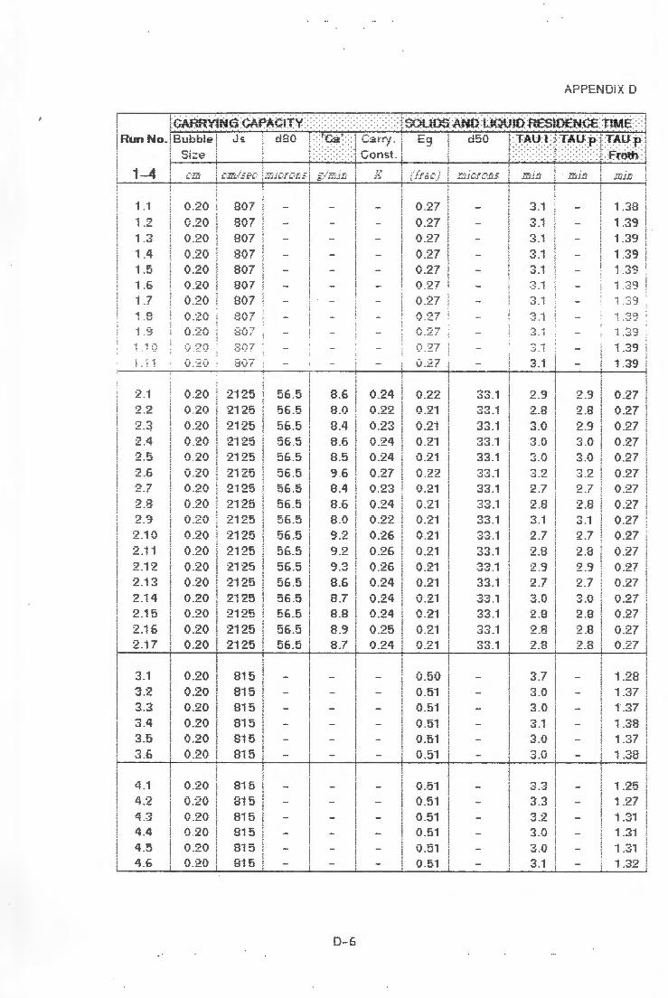
Run No. Bubble i Js d80

1-4

1 .1

1.2

1.4 i.5 1 .6

1.7 -, C : . '-1"

1 . '3

2.1 :2.2

2 .~ 2.4

2 .5

2 .6 2 .7 2.8 2.9 2 .10 2.i i 2.12 2 .13 2 .14 2 .15 2.16 2 .i?

3.1

3 .3

3 .4 3.5 3 .6

4 .1

,, ';) "'"'! .·J

4.4

4 .5 4 c..

l Size i

I ' i c.-m/5f·e: j1.;-s·ic.·.rc1;·s

0.20

0.20

0.20 0.20 0 .20 0.20 0.20 '!,..:· • .:... •..:

0 .20

-.._: _..:.·-.:·

! ! 807 !

:jUf

807 807 807 BO? 807

0.20 2125 0 .20 2125

0.20 2125 0 .20 2125 0 .20 2125

0 .20 2125 0.20 2125

0.20 2125 G.2(i 2125

0.20 2125 0 .20 2i 25 0 .20 2125 0 .20 2125

0.20 2125 0 .20 2125

0.20 2125 0.20 2125

0 .20

0.20

0 .20

0 .20 0 .20 0.20

0 .20 0 .20 0 .20 0 .20

0.20 0.20

815 815 815

815 815 815

815 815 0-i<: •J 1-...J

815

815 815

56 .5 56.5

56 .5 56.5 56.5

56 .5 56.5

56.5 56 .5 56.5 56 .5 56 .5 56.5

56.5 56.5

56.5 56.5

Ca' :

8 .6

B.O 8 .4 8.6 8 .5

9 .6 8 .4 8 .6 8 .0 OQ J . .:..

9 .2 0 ".) J .·J

8.6

8 .7 8.8

8 .9 8 .7

D-6

0 .24 0 .22

0 .23 0 .24 0 .24

0.27 0 .23 0 .24 0 .22 0 .26

0.26 0 .26 0.24

0 .24 0.24

0.25 r).24

0 .27

0.27 0.27

0 .27 0 .27 0 .27 0.27 r. "~~ ·-..:·.a:.. ,

0 .27

".J.~f

0 .22 0.21

0 .21 0 .21 0.21

0.22 0.21

0.21 0 .21

0 .21

0.2i 0 .21 r1 9 1 ___ , \J .21 0 .21

0 .21 0 .21

0.50 0 .51 0 .51

0 .51 0 .!:,1 0 .51

0 .51 0 .51 0 .51 0.5i

0 .51 0 .51

33 .1

33.1 ".)".) "i ·J,J . f

33 .i

33.1 .,,-. 1 ~~ -· 33.1 :.:-. 4 .;:;.:, _ 1

33.1 33.1

33.1 33 .1

33 .1 33 .1

33 .1 33.1

3.1

-...I.I

3 .1

3 .1 3 .1 ::: 1

3.1

,.., ~

>J . I

2.3 QO ~--~ 3 .0 ".) I'. -J. 'V

.-. r, .:., _•.)

3 .2 2 .7 2.8 3 .1 ' ) 7 ~-!

2.8 2.9 2 .7

3 .0 2 .8

2 .8 2.8

3.7 3 .0 3 .0

3 .1 3.0 3.0

3 .3

3 .0

-:i.V

3.1

APPENDiX D

1 .38

1 .39 1.39

1 .39 J :-.r .. i . .:r~

1 _::;9

1 .33

1 .39

2.3 0 .27 2.8 0.27

2 .9 0 .27 3 .0 0 .2? 3 .0 0.27

3 .2 0.27 2 .7 0 .27

2.8 0.27 3.1 0 .27 2.7 0 .2? 2.8 0.27 2 .9 0.2? 2 .7 0.27

3.0 0 .27 2.8 0 .27

2.8 0 .27 2.8 0.27

i .28 1 .37 ; ··:a

1.38 ~ ,.,.., I . >J:

1 .38

i .27 'i '01 ! .·J l

1.31 ... ?'1 ! .·J !

1 .32

Run No. Sparger Coll. 1-rnth Feed 1-'t

5-11

5 .1

5.2 5 .3 5.4 5 .5 5 .6 5.7

6 .1

6 .2 r ..., o . ..:,

6.4

7 .1 .... . 2 J

7 '3 l -~

7 .4

8 .1 8.2 8 .3

8 . 4

9 .1 9 .:2

9 .3

9 .4

10.1 10.2 10.3 10.4 10.5

10.6

11 .1 11 .2 11 .3 ii .4 11 .5 11.6

Type Hei9ht Height From Top

c;~·

SGDS 200

SGDS 200 SGDS 200 SGDS 200 :--r- ·,-1·--~ .... ~u~ 200 SGDS 200

SGDS 200

SGDS 200 SGDS 2 00 r-.. ,-. .-,. ,-. 200 u·"-~~·i::)

SGDS 200

SGDS 200 SGDS 200 c :~r.c 200 -...J'J.U ·~

SGDS 200

FCS 200 C ;~c 200 ! ".J....J

Fr~S 200

FGS 200

FCS 200 FCS 200 FCS 200 i::,-·c 2,-11\ . ...,~ vu

SGDS 200 SGDS 200 SGDS 200 SGOS 200 SGDS 200 SGOS 200

SGDS 200 SGDS 200 SGDS 200 SGDS 200 SGDS 200 SGDS 200

c-m

100

100 100

100 100 100 100

50

50 50

50

50 50 50 50

50 50 50 50

50 50 50 50

100 100 100 100 100

100

50 50 50 50 c." •JV

50

0-7

1 iO

ii 0 110 110 110 110 110

55

55 55 55

55 55 55 55

55 55 55 55

55 55 55 55

....... , I : v

110

1 i 0 110 1 i 0

110

55 55 55 55 c:;c. . , ... hJ

55

Voi.

F::ate

APPENDIX D

.................... .. ..... : '.: :- f EEi} {XJf.jl}fffOf:4 S: '. '. <

Solids ! Soiids I Grade i i

Rate l Density jMeasured I

Gr:ade

Ga~:: .

;"-1;}.'J]jJ);· J'_./J]j·Jfi :~f.: .(]Jl/~°"Jj ) i

754 81 .1

758 81 .1

753 81 .1

754 81 .1 -,.c.-. 8 .. ..; I ;JO I . I

762 81 .1 757 81 .1

1040 110.9

1079 1 i 5 .9 1099 119.0

1054 117 .7

1026 117.5

i089 117.4 1074 113.0

10·31 115.5

965 96 .3

960 99 .0 n. .. r: 93 .5 :, I ;_1

919 91.2

981 0-':> 7 U'\.J .f

984 91 .1 931 85.4

953 84.4

841 90 .8 1016 108.?

i292 140.3 1578 170 .6 1726 186.4

1958 210 .0

1119 117.6 ~ .. z-.r: 1 ...... ~. I I .:,;J I 7 . .:,

1101 116.8 1084 115.8 1080 -t'"i":!' ":1 • • ! . v

10.2

10.1 10_2

10.2 10.1 10.0 1 O. i

10.1

i 0 .1 10.2

10.5

10 .8 10_2

9 .9 10.0

9.5

9 .8 9 .7 9 .4

0 ~ ,_,. I

8 .8

8-7 r, ,. 0 . "1

10.2 10.1 10.2 10.2 10.2

10.1

! 9.9 !

i 9 .3 !

10 .0 ' i 1 O.i i

1 · 10 .2 ! ' '"' I . : lO uqq!nqj

2 .3

, ....... .:=. • ..:,

2.3 2 .3 2.3 2 .3

2 .05

2 .05 2 .05

2.05

2 .05 2 .05 2 .05 2.05

1 .73 1.?3

; -,~ ! . ! •..J

1 .80 1 .80

1.80

1 .80

2 .30 2 .30

2 .30 2 .3(;

2 .30

2 .30

2 .09

2.09 2 .09 2 .09

i .65

1.68

:2 .06 i .85

1 .91

1.97 1 .84

1.85

1 .93 2 .00 1 .84 2 .01

2 .08

2 .27

2 .08 2 .06

2.06

2.10

1 .70 2 .18

\"'3 en :=.... ,=_~

2.26

2.26

1 .90 1 .90 1 .82

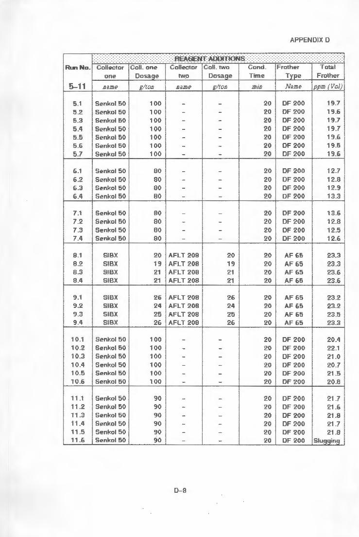
APPENDIX D

~::::::::::::::::::::::::::::::::::::::::::::::::::::~E.~~i~~~;N~:::::::::::::::::::::::::::::::::::::::::::::::::::::::::~::::: R!D! No_! Coiiector !Col!. one I Collector !Col!. two I Cond. IFrother I Total

I ! I I i i j one I Dosage I two I Dosage j Time I Type I Frother J f 1 l /T "f • 5-11 I fi i!JJJE" I _i'./t Ofi I 1:; i!Jl'i f2 _i'./t C<fi 1:,;;iii } i ;;;mE- I r,r,m .1 ·,, cd ,' I I""" . .. I ! I j

5.1 ! Senkol 50 I 100 I 20 DF 200 ! 5.2 I Senkoi 50 I 100 ! 20 DF 200 I 5 .3 i SenJ.;ol 50 j 100 I 20 DF 200 I 5.4 I Senkol 50 I 100 I 20 OF 200 ! 5.5 I Sen!.;ol 50 I 1 00 I 20 DF 200 I 5.6 I Senko! 50 ! 100 , 20 OF 200 I 5.7 I Senkol 50 I 100 I 20 OF 200 !

6.1

6.2

6 .4

7 .1

7 .2 -? [ _-..,

7 .4

8.1

8 .2 8.3 8.4

a -1 J.!

i 0 .1

10.3 10.4 i0.5

10.6

I Senkol 50 I i Senii::oi 50 i I Senko! 50 j i Seni-,ol 50 I

I . i ~en~~ol 50 I I ~eni,;ol 50 j

1 Sent".ol 50 I ! Senkol 50 ·

SIBX

SIBX SIBX SIBX

SiBX S!BX

SiBX SIBX

i i j Seni•;ol 50 I j ~en~~ol 50

1

,

1 ;:ienkol 50 j ~ I I ~n I ;:;en,m OlJ I i Sen!,:o! 50 I j Senkoi 50 i

I I

I Senkol 50

80

80 BO 80

I 20 I AFLT 208 i 1q i AFLT ?0° I - I ,-,. - o .

21 · AFLT 2oa I 21 I AFLT 208 1

I i 26 I AFLT 200 I 24 1 AFLT 208 I

I 25 AFLT 208 I ?6 j A F' T <:)r,n i - I'\ L .-vO ,

! i 0""' ! V ! 100 1

iOO ,:I

100 100 I

100 I

20 19 21 21

26 24 25 26

20

20 20

20

20 20 20 20

20 20 20 20

20 20

20 20

20 20 20 20 20 20

20

OF 200

OF 200 OF 200

OF 200

OF 200 DF200 DF200 OF 200

AF 65

AF 65 AF 65 AF 65

AF 65 AF 65

AF 65 AF 65

DF 200 DF200 OF 200 DF200 OF 200

OF200

19.7 19.6 19.7 19.7 19.6 19.5 19.6

12.7

12.8 10 Q

13.3

13.6

12.8 12.5 i2.6

23.6 23.6

23.2 23.5 23.3

20.4 22.1 21.0 20.7 21.5 20.8

21.7 11 .1 ii.2 11 .3 11.4 11 .5 11.6

;:)t'.lt', ;:J ii :---.-'-ol E::;o 90 ! 90 I 20

20 20 20 20

OF 200 OF 200 OF 200 OF 200 DF 200 DF 200

I 21 .6

I 21.8 , SenJ·,o! 50 I I Senkol 50 I I Sent,ol 50

1,

! Senkol 50 ;

:~ ,I

90 90 I

D-8

II 21.1

21 .8 !Slu9qinq

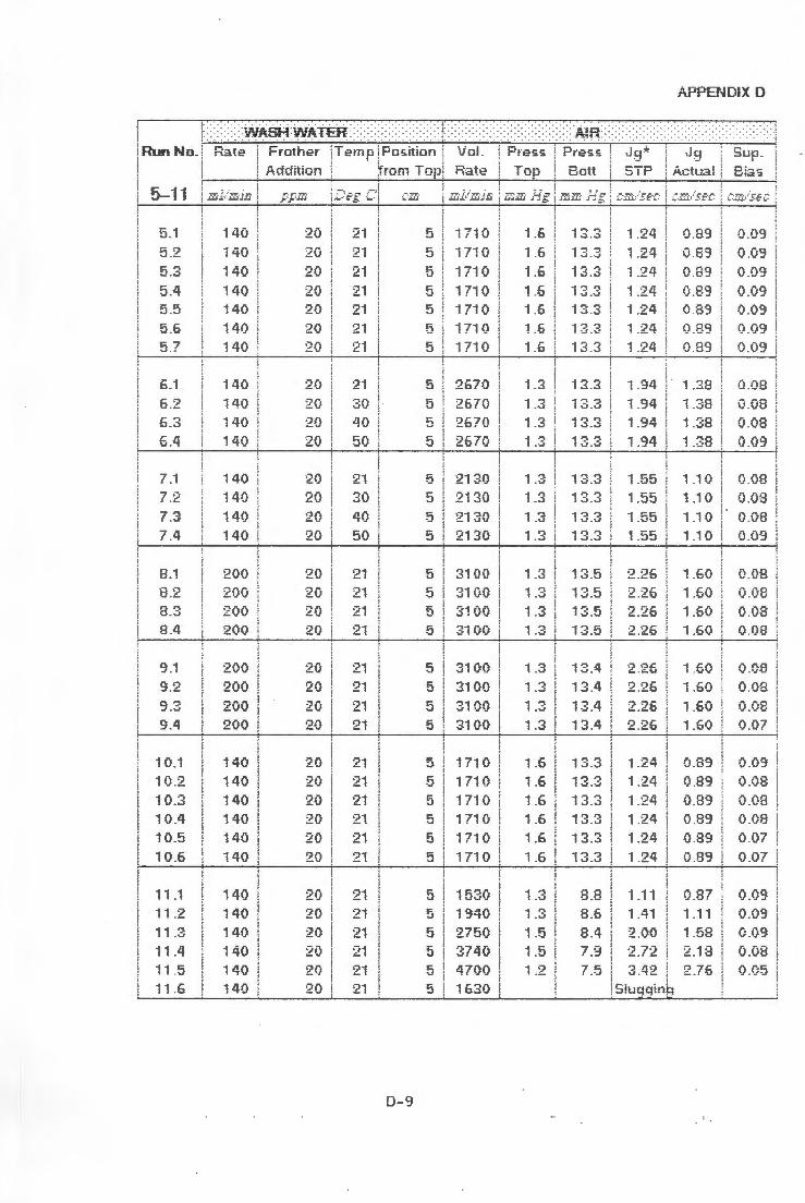
Run No.

5-11

5.1

5.2

5.4 5.5 5.5 5.7

6.i

6 .2 r r, D . ..:a

6.4

7.1 ~ .. j -~

"7 'Cl I . -..J

7.4

8.1

8.2 8 .3 8.4

9.1

9.2

9.3 9.4

i O.i

10.2 10.3 10.4 10.5 10.6

11 .1 11.2 11.3 ii .4 11 .5 ii .6

. . . . . . . ..... ... . ::: ::::::::WASH WAtER::::::: .... .. ..... . ......... . ..

Rate

I

1zl/ ;z·j1i' j

140

140

i 40 140 140 140 140

i 40

140 140 140

140 i40 -1 .. "'lr. I -Y"J

i40

200 200 200 200

200 200 200 200

140

140 140

140 140

140 i40

140 i40 140 140

20

20 20

20 20 20 20

20

20 20 20

90

20 20 20

20 20 20

20 20 20 20

20 20 20 20

20

20 20 20 20 20 20

2i

21 21 21 21 21 2i

21

30 40 50

30 40 50

21 21 .-.~ LI

21

21 21

21 21

21 21 21 21 21

21

:21 2i

21 21 21 21

-- -:---:--~-

D-9

5

5 5 5

5 5

5

·J

5

5

5

5

5

5

5

5

::;

5

5

5

5 r.: ;J

"' . .., 5

5

5 5

5 C ;J

5 5

Vol.

Rate i i ]:;:;,1,:]Z,jjj·

1710

1710

1710

1710 i 710

1710 i 7i 0

2670 2570 2670

2670

2130 2i30 2130 2130

310()

3100 :-.4 ,-.. r. ..:; l'JV

3100

-"J:~ r.i". •.J ! vv

3100

3100 3100

i 71 V 1710 1710 -17-i ."".

' ' IV

1?i0

1710

1530 1940

2750 3740 4700 1630

. . ... . .. ..... ·.· 1'::o. · .

. . . . ·.·.· . . ·.- .!"'.'!:!t .'l .',

!-'ress

Top

1.6

i.fi i ,• • 'O

1 r . . b

i .6

i .6

i.3 ~ ~ I . -.J

1.3 1.3

1 .3

i .3 -t 'Cl l .-.J

i ') . _..,

1.3

1 .3

... 'Cl I.-~

1.3 "1 ~ I·'"' i '"' . _..:,

1.6

1.6

1.6 1.5

i.6

1.6

1.3 i .3

1.5 1.5

Bott

i r, r, . .:. . ~

I ·.J .·J

13.3 ... :-. r. &.:.,_.:,

; "':\ ·':\ !•..: .-..:

i 3.3

13.3

13.3 i 3.3

i3.3

13.5

13.5 13.5

13.4

13.4

i 3 .3

13.3

13.3

8.8 8.6

8.4 7.9 "7 ,:;_ ! .·J

APPENDIX 0

Suo . •

Jg STP Actual

1.24

i .24 1.24 1 .24

1 .:24 1 .24

1 .94

1.94 1 ea.-, . __ ., 1.94

1 .55

i.55 1 .55 1.55

2.26

2.26 .-. .-. .,,-.:: . .c:.o

•"'l •"".lC. ~ -~\.]

2 .26

2.26

i .24 1.24 1 .24 1 .24 1.24

1.24

1 .11 1 Ai

2.00

2.72 3.42 ! l

S!uqqin~

0 .89

0.83

0 .89

0.89

0 .89

i .38

1.38

1.38 1.38

1.10 i .10 1.10 i .iO

1 .50 1 _E,()

1 .60

1 .60 1 .60

1.60 1.60

0.89

0.89 0)39 0 .89

0 .89

O.B? i .i i

1.58 2.18 2.76

0.09

0 .09

0 .09

0.09 0.09

0.09

0.09

0 .08

0.08

0.08

0.09

0 .08

0 .08 0.08 0 .09

0.08

0.08

0 .08 0 .08

0 .08

0.08 0.07

0.08 0.08 o.oe 0 .07

0.07

0.09 0.09

0.09 0.08 0.05

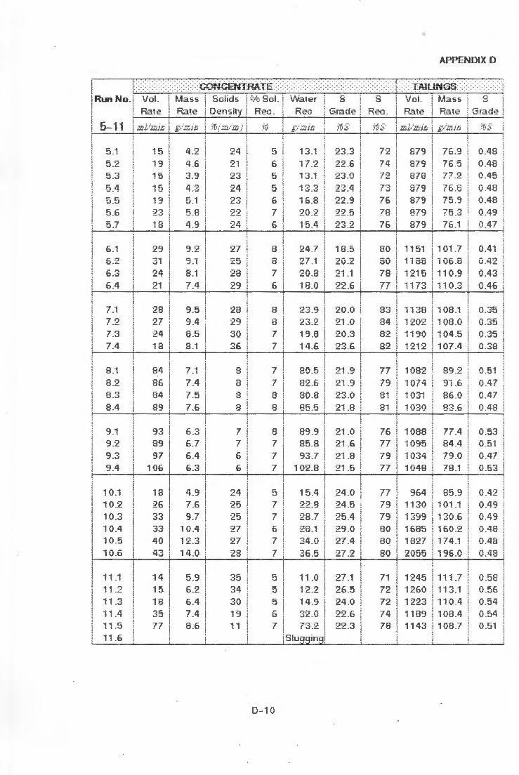
:::::::::::::: :::: ::::: :::: c.0t-°.iCENTP.A:TE::::: Run No. Vol.

Rate

Mass ! Solids C</c, Soi. Vi.ater S S

Rate I Density Rec. Rec Grade Rec.

Vol.

Rate i

APPENDIX 0

Mass S

Rate Grade

:~It s: r:;·1, 'J .. ::J.!i j g./ JJj'jjj

5 .1

5 .3

5.4 5.5 5.6

5 .7

6.1 6.2 ,- :. c . .:,

6.4

7.1 7.2 7 ':l ! .,J

7.4

8.1

8 .2 8 .3 8 .4

9 .1 9 .:2 9 .3 9.4

1 fl 4 ~-' 10.2 i 0.3

10.5

10.6

11 .1 11.:2

11.3 ii .4 11 .5

11 .6

15

19 15

15 4 ,._

I ':J

18

29 31

24 21

27 24 i8

84 86 ..-... , O"t

89

89 97

106

18 26 :-,r., .:,.:,

':>':l ,_.-.J

40 4-:, ...,

14 15

18 35 77 I I

4.2

4 .6 3.9 4 ·';'

• • -.J

5.i

5 .8

9.:2 9.1 8.1

7.4

9.5 9.4 0::; ._, _....,

8 .1

7.1

7.4 7 .5 7 .6

6.7

6.4 6.3

4 .9 7 .6

9.7 10.4 1 •:> "' ·---=>

14.0

5.9 6 •j

6.4

7.4 0 r u.t>

24

21 23

24 23 22 24

27 25 28 29

28 29

36

8

8 _.., 0

8

7 7

6

6

24

25

:27 28

34 30 i9 11

5

6

5

5 6

7 6

8

8 ...., t

6

8

8 7 7

7

7 8 8

8

7 f

7

5 7

7 6

7

7

5

5

6 7

0-10

-;, "J ! ! . ::...

13.1

13.3 .. r r. I 0 . 0

20.2

i 5.4

24 .7 27 .1

20 .8 18.0

23 .9

19.8 14 .6

80.5

82.6 80.8 85 .5

89.9

85.8

93.7 102.B

15.4 22.8 28.7 ~"".30 -t ::..•J.l

34.0

36.5

11.0 12.2 14.9

32.0

S!uqqinq!

23 .3

22 .6 23 .0

23.4 22 .9 22 .5

18.5

20.2 21.1

22.6

20 .0 21.0 20.3 23.6

21.9

21 .9 23.0 Q-1 0 ~: -~

21 .0 :21.6

21 .8

24 .0 24 .5

25.4 2'J .O

:27.4

27.2

27 .1 26.5

24.0

22 .6

72 74 72 r~ ·.J

76 78 76

80 80 78 77

83 84 c~~ IJ.C...

8:2

77 79 .-... 01

81

76 77 79 77

77 79 79 01\ '.JV

80 80

71 72 72 -, 11 I "t

78

879 879 .-.,n o;o

879 879

879 879

1151

1188 1 •:>1 i:; • - • ;J

1173

1138 1202 1 i90 12.i 2

1 /iQ•:;i

1074 1031 1030

1088 1095

1034 1 /i!J.n

I U 10

%4

1130 i 399 1585 1827 2055

1245 1:260

1223 1189 1143

I

76 .9

76.5 77 .2

76 .8

76.1

! 101 .7 i - -- D ! IVb .u

i 110.9 I

! 110.3

i ; 1 ~o 1 j s l}·~-

i 108.0 ! 104 5 i . ! 107.4

I

89.2

91.6 86 .0 0'"' r ·~~ -b

77 .4 84 .4

79.0

78.1

I 85.9 ! 101 1 : - - - - -

! i30 .6 j 160.2

1 174 .1 i 196 .0 ! I ! 111 .7 1113.1 ! -1-1 /) 4 • s t - - • I l 108.4 l 108 .? I

0.48

0.48 0.45

0.48 0.48

0.49

0.47

0.41

0.42

0.43

0.46

0 .35 0 .35 0 .35 0.38

0 .51

0.47 0 .47 0 .48

r. ::;-~ v.-_•-..!

0 .51

0 .47 0 .53

0 .42 0.49

0.49 0 .48 0.48

0 .48

0.58 0 .56 0 .54

0.54 0.51

Run No :nu'-bt- : le r1Qri • j C) u .t- : u.., ..... --

5-11

5.1

5.2

5.4 5.5 5 .6 5.7

6 .1

6 .2 6 .3 t=-4

7~ : • I

7 ·~ J • .:..

7.4

8 .1 8 .2 8.3 R4

9 .1 9 .2

9 .3

i O.i

10.2

10.3 10.4 10.5

10.6

- 1 -' '. !

11 .:2 11 .3

ii .4 11 .5

! Size I

0.15 i780

0 .15 1780 0 .15 1780

0 .15 1780

0 .15

0.15

0.15 0 .15 0 .15

0.15

/'·, -f {:;, ..... . ! •_j

l 0 .15 : : O.i5 ·1 0 .15 !

1140

i 140 1140 1, =W

1140

1833

2493

11 .6 SluqqinA

43 .3

42 .6 39 .0

:36.5

38 .0

42 .6

48 .4 48 .4 52.2 ·.J·-~. _,,.

:31 _5 52.7 43 .8 46.1 ~":\ 0 •J•..J.U

~ ¢ii:: Garry .

·:J .2 9 .1 8 .1

7.4

7.6 97

12.3

b.:i

6.4 7.4 0 ~ ._,_;:;

D-11

Const.

0.4 0 .4 0.4

0.4

0.4 0 .5

0 .6 Q.6 0 .7 ~ ":'-··-·

0.6 0 .3 0.2

0.2 0.2

APPENDIX 0

Eq d50 [ :l)\f)Y !: TAO:pJ TAO:i:1: - ~ :. : : : : : : : : : : : : } :: : : : : : : : : : : : : } ::F.:1:i:ii:1; ::

I !

( l~"Bt) i J?J)CIC:JJS i 1IiJJj·

0.24

0.24 0 .24

0.-24 0 .24 0.:24

0.24

0 .22

0.22 0.22

0.22

0.23

0.22 0 .22 0.22

0.21

0.21 0 .2:1

0 .21 0 .21

0.21 0.21

0.24 0.24

0 .24

0 24

0 .53 0 .55

0 .59 0.59

20 .9 20 .9 19.9

19.7

19.0 20 .3

22.1

25 .5

25.7 22.2

24 .2

4 .0

4 .0 4.0

4.0 4 .0 4 .0

4 .0

3.1

3 .0 2 .9 3 .0

3.1 3.0 3 .0 2 .9

3 .4 .-, C .:. .~

3.5

':> ':> ·.J .·-1

3 .5 3 .5

" ,.. ..:, .o

3 .1 2.5 2.1 1 .3

1.8 1.7 1.7

i .6 1.6

1:j·j :,".;·

3.1

3 .0 2 .9

3.6 3J 2.5 2.1

1 .8 ~ -, l • f

1.7 1 .6

i ~.~. . _.:,.:,

1 .32 1.33

1 .33 1 .32 1 .32

i .33

0.42

0 .42 0.42

0.43

0 .53

0.53 0 .53 0.53

0 .36

0 .36 0.36

0 .36 0.36

0 .36

0 .36

i.33 1 .31 i .31

1 .31 ~ .31

. ' ! . ·..I I

0.74 0.53 !).41

0.30 0 .24

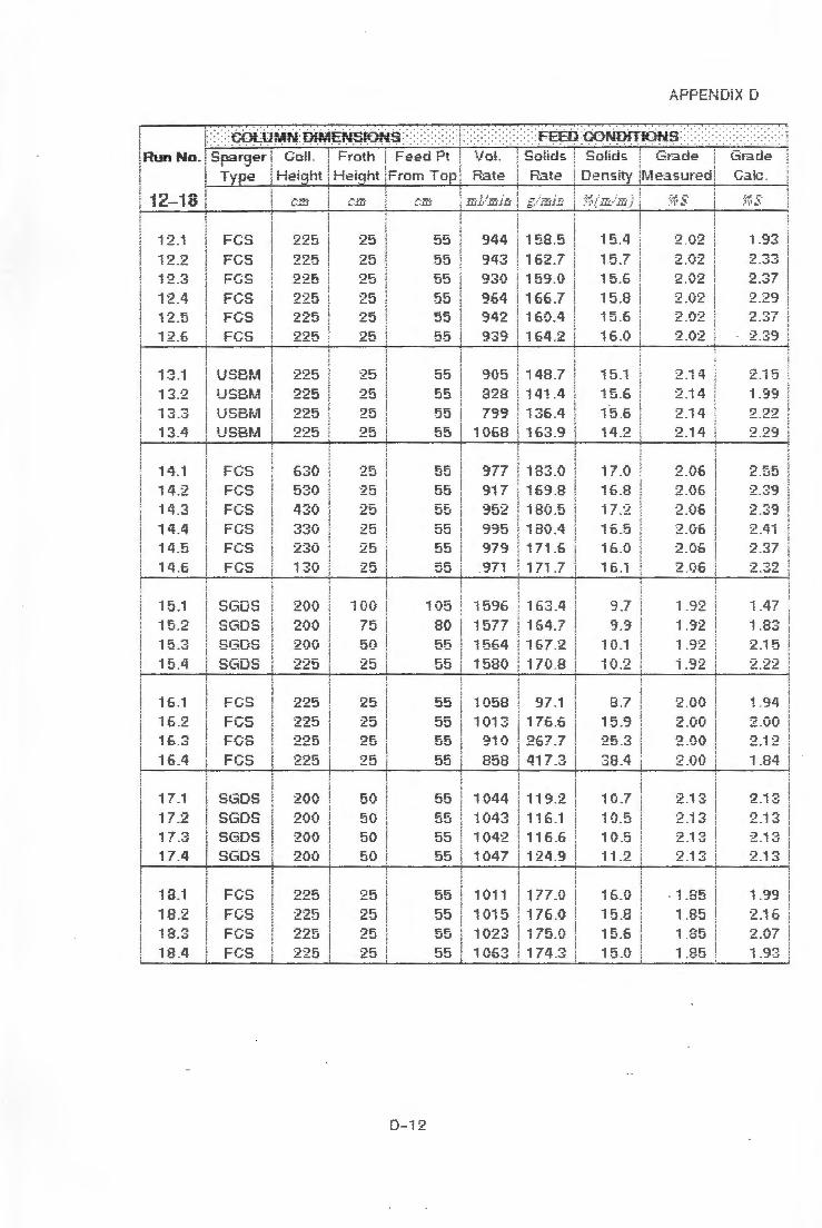
Run No. Sparger Goll. Froth Feed Pt Vol.

12-18

12.1 '1? ry t .:- . .:..

12.3

12.4 12.5 -j Q £: !.:.. . ~

13.2

13.3 .. -. ,, l.:J . "1

.. ,'1 ... I '"t. I

14.2 i 4.3 14.4 14.5

14.6

15 .1 15.2 15.3 i 5.4

i 6 .1

15 .2 1 C. ~. ~ . .:,

16.4

17.1

17.2 17.3 17.4

18.1

18.2 i8.3 18.4

Type Height Height From Top Rate

FCS FCS FCS FGS ,-4'-. :""",. r·v~

FGS

usm.,1 USBivi

FCS FGS FCS FC;S FCS FGS

SGDS SGDS SGOS SGOS

FCS FCS FCS FCS

SGDS SGDS SG.DS SGDS

FCS FGS FGS

FGS

225

225 225 225 225 225

225 225

225 225

630 530 430

230 130

200 200 200

225

225 225 225

200 200 200 200

225 225 225 225

25 25 25 25 25 25

25 25 25 25

25 25 25 25 25

25

100 75 50 25

25 25 25 25

50 50 50 50

25 25 25 25

D-12

55

55 55 55

55

55

55 55

55 55

55 55

55

105 80 55 55

55

55 cc ..,.., 55

55 .:: r= ;J;J

55 55

55 55 55 55

944

943 930 964

939

905 828

799

1068

977 917

952 c.oc::. JJ -..!

979

971

1596 1577 1564 1580

1058

1013 es~ n -Iv

858

1044

i043 --: r . .n ~; !'.?,~

1047

1011 1015 .. f','J~-J '1..._.:,

1063

APPENDiX D

: : FEED :G--0~~t;-tff{j~JS: '.:::::: .... . ... . . ... . ....

Solids ! Solids l Grade Grade

Rate I Density iiv1easurect Ga~:: .

158.5

162.7 159.0

166.7

164.2

""1 ltC 7 ! -Y•..I . I

141 .4 136.4

183.0 169.8 180.5 180.4 171.6

17i .7

163.4 154.7 167 .2 170.8

97 .1

176.6 267 .7

41? .3

119.2 116.i ~ "i C ~ I f v .ti

124.9

177 .0

176.0 175.0 174.3

15.4

15.?' 15.6

15.8 ~,: ,. I ;J . 0

16 .0

-ih -t t ·.J . I

15.6

15.6 14 .2

17.0

16.B i 7 .2 16 .5 16.0

16 .1

9 .? 9 .9

10.1 i0.2

8.7

15.9 25.3

38 .4

10 .7

i0.5 -tr. rt v .=:1

11 .2

16.0

15.8 15.6 15 .0

2 .'}2

23)2

2 .02 2.02 2 .02 2 .02

·-~ "'1 ... , .:.. . ! -r

2 .14

2 .14 2.14

2.06 ,:i r.c ~ - "'J~

2 .06 2 .06 2 .06

2.06

~ .-.. ~ l . :::JL

-j ()C} t .~.::..

... ,-... -, J _:,~

2 .00

2.00 2 .00

2.00

2.13 2.i3

2.13

1.85 1.85 1 .85

? ?':' - . ,JJ

.-. '"'7 ;::__.:, ,

2.29

2.39

2 .15 1.99

2 .22 2 .29

2.55 2 .39

2 .39 ~") .. '1 "'1 a:... . "'l' t

2 .37

2 .32

1.47 ~ .-.J""I, 1 .00

2.15 2 .22

i .94

2 .00 2.12

1 .84

2.13

2 .i 3

1 QQ

2 .16 2 .07 1 .93

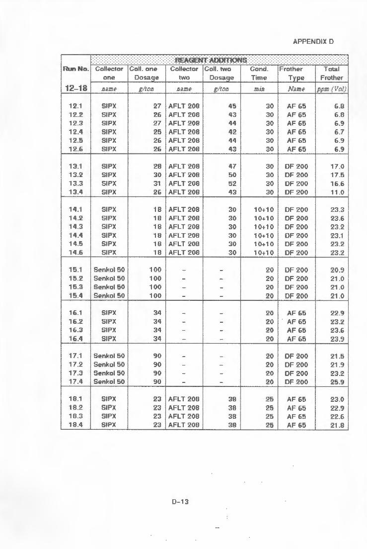
Runf-4n.

12-18

i 2.i 12.2 12.3

12.4 12.5 12.6

13.1 i3.2 13.3 13.4

i 4.i 14.2 14.3 14.4 i4.5

14.6

15.1 15.2 15.3 15.4

i6.1 16.2 16.3

16.4

17.1 17.2 17.3 17.4

18.1 18.2 ..:r. :"'\, 10 • .:;

18.4

APPENDiX D

::::::::::::::::::::::::::::::::::::::::::::::::::::~~t~~~~fii$::::::::::::::::::: Collector !Goll. one Golie-.:;tor Go!!. two Gorn:!. rrother I Tot:;.i

one I Dosage two Dosage Time Type ! Frother

S!PX

SiPX SIPX

SIPX SiPX SIPX

SIPX SiPX

SiPX SIPX

SIPX S!PX

SlPX SiPX SIPX

SIPX ! I

Senkol 50 I Senl,;oi 50 I Senko! 50 I Seni-:oi 50 !

SIPX

SiPX SIPX SIPX

I Senkol 50 I Sen~;ol 50 i Senkol 50 j Senkol 50 i

SIPX

S!PX SIPX SIPX

g./tC:15·

27 26 27 25 26

28 30

31

iB 18 iB 18 18

18

100 iOO 100 100

34 34 34 34

90 90 90 90

AFLT 208

AFLT 208 AFLT 208

AFLT 20B AFLT 208 AFLT 208

AFLT 208 AFLT 208

AFLT 208 AFLT 208

AFLT 20B AFLT 208 AFLT 208 AFLT 208 AFLT 208

AFLT 208

23 AFLT 208

23 AFLT 208 23 AFLT 208 23 AFLT 208

D-13

45 43 44 42 44 43

47 50 52 43

30 30 30

30

30

38 38 38 38

30

30 30 30 30 30

30 30

30 30

i0+10 10+10 iO+iO 10+10 i0+10

10+10

20 20 20

20

20

20 20

20

20 20 20 20

25 25

25

AF 65

AF65 AF 65 AF 65 AF 65 AF65

DF 200 OF200

DF 200 DF200

DF200 DF200 OF 200 OF200 OF 200

DF200

DF200 DF200 OF 200 OF 200

AF65

AF 65 AF 65

AF 65

DF200 OF 200 OF200 DF 200

AF 65

AF65 AF 65 AF 65

I i.,r,_p.'j~· (t7c}}

6.8 6.8 r ,.. D.:1

6.7 6 i:';

6.9

17.0 17.5

16.6 11.0

........ :"\ ~.:) . .:)

23.6

23.1 23.2 23.2

20.9 21.0 21.0

2i.O

22.9 23.2 23.6 23.9

21.5 21.9

25.9

23.0 22.9 22.6 21.8

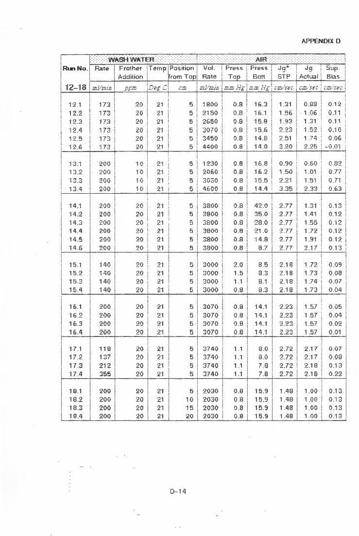
Run No.

12-18

12.1

12.2 12.3 12.4 12.5 12.6

13.2

13.3 .... - • .-"l JV. '"'1

... -: .; l"t.l

14.2

i 4.3

14.5

14.6

15.1 15.2 15.3 i 5.4

16.1

16.2 16.3 16.4

17.1 17.2 17.3 17.4

18.1

18.2 18.3 18.4

Rate ! Fro1her jTen1p 11Posi!ion : .• Vol.

! t..c:r:;,;u-11 ! ,...._ H.-IIU rrom Topi Rate i

JZ·i i'i-1;·ifj i

173

173 173

173

173

200 200 200

200 200 200 200

200

140 140 140 140

200

200 200 200

118 1 '=!7

355

200 200

200 200

20

20 20 20 :"\.,-.. LV

20

10

10

20 20

20

20 20

20

20

20

20 20

20

20

20 20 20

20 20 20 20

I i i

!L)f·g -Cj C-'i·Zi I :.-:Z·l,:~"j"jjjj'

:21

21 21 21 21 21

21

21 21

21 21

2i 21 21

21

21 21

2i

21

21 21 21

21 21

21 21

21

21 21

D-14

5

5 5 5 5

5

5

5

5

5

5

5 5 5 5 5

5

5 5

5

5 5 5

1800

2150 2650

3070 3450 4400

i '230

. .:;u . .:;v

4600

3800 3800

3800 ·-:lOl'.,f'. ·-·•.J~J"J

3800 3800

3000 3{)00

3000 3000

3070

3070 3070 3070

5 3740

5 3740

5 3740 5 3740

5 2030

10 2030 15 2030 20 2030

Press

Top

o.a 0.8 0 .8

0.8 0.8 0.8

o.e 0 .8

0 .8

0.8

0.8

0 .8

0 .8 0.8 0.8

0 .8

2.0 1.5 -! -! '.' 0 .8

0 .8

0 .8 0 .8 0.8

1 .1 ; .i

1 .1 i .1

0.8 O.B f• :-. J.O

0.8

.... . .. . .

. ·.·. :no. · . . ·. : --~!! .tt ,:.

Press J9 Bott STP

1 b.3

16.1 15.8

15.6 ... .;; .-. l"t .O

14.0

16.2

15.5

14.4

42 .0 35.0

28.0 21.0 14.8

8.7

8.5 r. ,-. c.~ 0-! ._. _ !

,-.. -. o.~

i 4 .1

14.1 14.1

14.1

x 0

8.0 70 ! _._,

7.8

15.9 15.9 15.9 15.9

1 .31

1 .56 1 .93

2.23 2.51 3.20

0 .90 1 .5()

2.21 3 .35

2.77 2.77 ,:; 7'7 ~-· f

·."'J. 77 ::.. .I I

2.77

2.77

2.18 2.18 ,:, -!O J:....t•..!

2.i8

2.23 ~ ~":', .::.. • .:.:...-..1

2.23

2.72 2..72 2.72 2.72

1.48

1.48 i .48 1 .48

APPENDIX D

jg A.ctuai

0.88

· 1 .06 1 r-,; . . ,..:, :

1 .52 i .74 2 .25

0 .60

1 .01

1.51

2.3:3

1 .31 1 .41

i.55 -t --r~"'J. J . /.::..

i .91

2.17

1.72 i .73 1 .74 i .73

i .57

1 .57 1.57 1.57

Suo . I

Bias

0.12

0 .11 0 .11

0.10 0 .06

:"'\ C -.'"l .. ~- .•.J.:..

0 .77

0.71 0 .63

0.13 0 .12

O.i 2 0 .12 0 .12 V.! .J

0.09 0 .08

0 .0?

0.iJ4

0.05

0.04 0.02 0.01

2 .1? 0 .07

2.17 0.08 ,:, -! 0 ,., -! ~ ::... !U V.t·J

2.18 0 .22

1 .00 0 .13

1.00 0.13 1 .00 0 .13 1 .00 0.13

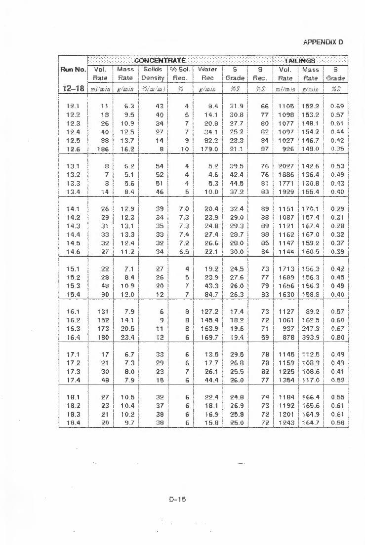
. • :G,.?f..l{;ENTP.A T:~• • •. • • •: ·. Run No. Vol. Mass \ Soiids O/c Sol. s

i 2.i 12.2

i 2.4

12.6

13.1 13.2

13.3 13.4

1 /I Q -~-~ i 4.3 -t: .:'! ..,., •=-~ i 4.5

14.6

15.1 i 5.2

15.4

16.1

16.3

16.4

17 .1

17.2 17.3 17.4

18.1

18.2 18.3 18.4

Rate Rate ! C1ensity Rec .

18 26 40 88

C 'J

7

8

14

26 :29

31

32 27

22 :io

48 90

i 3i

152

173

180

17

21 ':>A •JV

48

6.3

9 .5 10.9

J .-. -:r I .::,. f

16.2

5.2 5.1 ;;:;, C. ·...J . V

i 3.1

12.4

11.2

7 .1 8 .4

10.9 1 'J fl

7.9

14.1 20.5

23.4

6.7 7 ~. f • .:.

8 .0 7 .9

27 10.5

23 10.4 21 i 0 .2 20 9.7

43

40 34 27

8

52

51 45

33 34 35

.-.. ']" .:,_

34

27 26 20 12

6

9

11

12

33

15

37 38 38

4

7

4 4

4 5

7 .0 7.3 7.3 7 /I ! _..,.

7.2

6 .5

4 5

7 7

a 8

8

8 .4

14.1 20 .8 34.1 82.2

179.0

5 .2 4.6 :) .-.:i

10.0

20.4

24.8

26.6

22 .1

19.2 23 .9 43 .3 84.7

127.2

145.4 163.9

3i .9

30 .8 27 .7

25 .2

21 .1

42 .4

44 .5 37 .2

:29 .0 29 .3 ~~o 7 ,:_ '.J. !

28 .0

30 .0

24.5 27.6 2£ .0

i?.4

18.2

19.6

6 169.7 19.4

6 6 f

6

D-i5

6

6 6

13.5 29.5 17.7 26.8 26 .1 25 .5 44.4 26.0

22.4 24.8

18.1 26.9 16.9 25.8 15.8 25.0

s Rec .

66

77

APPENDIX D

. ... . ... . ....... . . .. . ... . ' . ... . . . . · . . - "T-::'\ "11 - J.LJCC - . ·. · . . -: -:- : - ~ -~1~~~9:~~ - : -.

i'o! i t.1tass '.J • ! s Rate j Rate Grade

1105

1098

! i 152.2

i 153.2

0.69

0 .57 80 1077 ! 148.1 0 .51

' 82 1097 ! 154 .2 0.44 8~ 1027 j i 46.7 0.42 87 926 l 148 .0 0 .35

ft:. 2027 ! 142.5 0 .53 76 1886 ! 136 .4 0.49

81

.-.. -. 0~

88 89 ca •-1•...1

85 84

73 77 79

83

73

72 71 59

1771 1929

i 151 1087 1 i 21

1147 1144

1713

1656 1630

i 127 1051

937

i 130.8 j 155.4

j i70 .i I 157.4

i 167.4 i -i C.7 /\ 1 l U! . 'J ' i 159.2 l

j 1 fi0 .5

i j 156.3 J ~ r-:r .-. \ I JQ . .j

i 156.:3 I

! i58.8 j

j l Q•:C .:, l ___ ._

I - -- -! i b~.!.J

i 'J47 r, ' - ., • .:> I

0.43 Ct .40

0 .23 0.31 0.28 0 .32 0 .37

0 .39

0.42 0 .45 0.49 ().40

0 .57 Q.60

B78 i :393.9 0 .80

78 1145 112 .5 0 .49 78 1159 108.9 0.49 82 1225 108.6 0.41 77 i 354 i i7 .0 0.52

74 1184 i 66 .4 0.55 73 1192 165.6 0.61 72 1201 164 .9 0 .61 72 1243 164.7 0.68

Run No_ ! Bubble ! I l

i Size ! 12-18 l C:1Ii

12.i

12.3

12.4 i 2 .5 12.6

1 3 .2 S?? I ·J.-.J

1,.., .,, , ..:; . ~

~ .. , ... I '"t .l

14.2

i 4.3

1 " r,: ... . CJ

14.6

15.1 15.2 15.3

i 5.4

16.1

16.2 ... r ..-. ; ;;,_..:,

16.4

17.1

17.2 ~ 7 .-:,. I / . -.J

17.4

18.1

1B.2 1 .-. :-. lO . .:>

18.4

0.21 870

0 .20 1059 0.21 1280

0 .21 14B3 0 .22 1590 !) .22 2028

0 .22 569 0.20 i 030

0 .17 1751 0.20 2277

0 .20 i 900 0 .20 1900

0 .20 i900

0 .20 1900

0 .20 1900

0 .1 5 0 .15

0 .15

2000 2000 2000 2000

0.20 1535

0 .20 1535 0 .20 1535

0.20 1535

0 .15 2493

0 .15 2493 0 .15 n .. 10":l

.::...-YJ....J

0 .15 2493

0 .20 1015

0 .20 1015 0.20 1015

0 .20 1015

54 .5

51 .4 50.3

56.8 53 .7 54.7

50.7 50.0

40 <"} u.::..

47 .9

56.5 49.0

48.6 t=.7 .n.. -...!I .V

49 .4

55 .8

51.2

66.6

60 .7

30 .1

53.9 53.4

67 .9

48.5

41.4 55 .7 57 .0

r,.~ {\ c .... v

81 .8 82.5 84 .4

6 .3

9 .5 10.9

i2.5 13.7 16.2

5.1

5.6 8.3

13 12 i3 -I".:> I ._,

12

i1

7 .1 8.4

10.9

i2.0

7.9

14.1 •:)t\ J::; .... v . ~

a"J":\ ~'*.J-4

6.7

7.3 8 .0 ? .9

10.5

10.4 10.:2

9.7

D-16

,-:arnJ ;

~G~~t-. !

0.47

0.62

0 .60

0 .52 0 .55 0 .50

/\ 77 -..f .I I

0.35

0.23 0 .26

r, ~~ ~-~• 0 .60

0.60 l\ ... 1 C. v.-,,v

0.44

0.31

0 .21 0 .22 0 .24 0 .30

0.58

0 .58 0 .85

0.76

0 .17

0 .21 0.17 0.17

0.44 0.44

0 .40

Eg

0 .13

0 .14 0.16

0 .17 0.22 0 .27

0 .07 0 .11

0 .15 0.21

0.18 0 .19

0.21 _,._ ~"'J: ":l-t.J . i:... •.J

0 .23

0.23

0 .58 0 .56

0 .57

0.23

0 .26 tJ .30

0.36

0 .56

0 .55 0 .57 0.57

0.15

0 .15 0.15 0 .15

d50

30.2

27.8 .--.r, ~D.t

30 .8 27.4 25.2

27 .6 27 .0

26.3 24.8

24.1 23.2

33 .7 25.0

24.7

29 .1 97 r· - · .'J

i? .O

25 .1

31 .3

24 .4

20.3

33 .8

40.4 40.7 41 .1

42 .4

APPENDIX D

f ~AU:U .TA!J>tlf TAU.n: ~ ... ·: · •: •: •: • t ... • .. •: • • :·: • J:: i.n1th::

4.1

4 .0 tl .O

3.9 3 .~

4 .1

2.4 2 .4

2 .5 2 .1

10.3 Cj -I - . ' 7.0

5 .0 3 .5 ,:;.. . v

1 .1 i .2 1 .3 i .4

3.5

3 .6 3.9 .... ~ . .:, . ti

1 .8

1 .8 1 .6 1.5

3.7 3 .7 3 .6 3 .5

4 .0 0 .32

4 .0 0 .26 4 .0 0.21

3 .9 0 .18 3 .9 r) .16

4 .1 0.12

2.4 0.46 2 .4 0 .28

2.5 0.1 9 2 .1 0.12

10.3 0.1 5 9.1 0 .15

7 .0 0.15

5 .0 0 .15 3 .5 0.15

2.0 0 .15

1 .1 i .2 1 .3

i .4

3 r-,

3.6 3.9 3 .8

1 .8

i .8 ~ C: I . U

1 .5

" ..., ,:; _: .... ..., .j. I

3.6 3 .5

U. i b

0.57 0 .38

O.i9

0 .18 -~o t.J. I '.J

0 .18

0 .1B

0.30 0.30 0 .30 0.30

0 .28

0 .28 .. , .-...-. v . .::.o

0 .28

A!-'!-'i::.NUiX i.J

Run No. Sparger ! Cai!. ! Froth ! Feed Pt Vo!. Solids I Solids j Grade , Grade

Fate i Density jivieasured j Ga~::.

19-22 i

i 9 .i

19.2 19.3

2-J.1

20 .3

2! .1

21 .:2

22.1 ,.,,., ,, .::....::....i:..

22 .4

Type i Heiqht j Heiqht jFrom Top R.ate

FCS FCS FGS

SGDS S!.308

SGDS

FGS ! V·-'

FGS

FGS

FCS FGS

[ ::I,i

225 225 225

200 200 200

225

· .. ··.- .-. ._.._._:

225

225 225 225 ::'J,~"'.) ~ ~-=-v

25

25 25

50 50 50

'25

25

25 25 25 25

0-17

55

70 85

55 55 55

55

·-· ·-·

55

55 55 55 55

·-· :- .:·--1· - - l ,. .... -1· •• .·,·_-'(,_.;:-'J"':· , ...... ,·.,·.,·.· .• ,! ·1

1• ;";"; ;:• .t.;''.i .:-.;- £ :' J.J.i Ji • --

1 Oi 1

1046 1 Ot:4

1082 1024

1012

i 77 .0 ~ 7-; "'1 ! ! ! . f

176.4

122.1 115.8 117 .4

.-~ -i .- . -::; ;. . .::.

. - ..... .... -; •.:· .:.. .•..!

88.7

1109 102.9 974 76 .0

·325 i 69 .3 880 160.5 889 16i .5

892 160 .6

16.0

i 5 .5 15.3

i 0 .6 10 .6 10.9

8 .3

6.6

8 .8 7 .5

16.6 16 .6 16.5

16.4

i .85

1 .85 1 .85

2.65 9 ii .-• ..; -i ~. ; :

:2.:28

2 .28 2.28

2 .05 2 .05 2 .05

2 .05

2 .25

2 .i 5 2.19

2 .30

1.72.

1 .97

~- ! -~

2 .27 2.35 2 .8:7

2 .03 2.31 2.24

2 .2fi

APPENDIX D

1:::::::::::::::::::::::::::(:::::::::::::::::::::::::~f ~~w.r;.~::::::::::::::::::: :::::::::::::::(:::::::::::::::::::::::::::~ RunNo_ l Collector Goll. one Collector 1col!. two Cond. Frother

I Total

I Do-sacte Time T Frother I

! one two i Do-sa e e I

19-22 I r,·;,·me- g/tCifJ' r,·amf· g/t c.-.fi .J"j:;-j,Jj l'i/iiJl'iE· j pp1,:;· { V C<]) I I AFLT 208

! I

I i9.i S!PX 22

I 37 30 AF 65 23.0

19.2 51PX 22 I AFLT 208 37 30 AF65 22.2

' 19.3 S!PX 23 38 30 AF 65 22.0 I 1 AFLT 208 I I

I

i 2:0.i HSO {pH=3.8} I Senl<:ol 50 100 30 OF 200 21.8 I ! 20.2 HSO (pH=8.0} I Senr.:o! 50 100 30 DF 200 21.9

I 20.3 HSO (pH=8.0} I Senkol 50 ! 100 30 DF 200 22.0 I I

I I 21.i S!BX 9.8 I

I 40 AF 65 23.1 I I

2i.2 5iBX I I 21 .7 40 AF65 22.7 I 21.3 S!BX 42.2 I 40 AF 65 ':)"1' ~-

I ~v . .:

I 21.4 SIBX 60.7 I I 40 AF 65 22.8 21.5 SIBX .. ,..,, .. = I i 40 AF 65 :-..r.. r.. I IL I • .J I .t:.,.:;_.:;

I I I 22.1 SIPX I AFLT 208

i 25 I 42 I 30 AF 65 5.3

I 22.2 SIPX 26 I 44 I 30 AF 65 10.0 I AFLT 208

I I 22.3 S!PX 26 AFLT 208 44 I 30 AF65 14.9 I 22.4 SiPX

I 26 i AFLT 208 I 44 I 30 AF65 19.6 I

D-iB

Run No.

19-2"2

19.1

19.3

.-.,,.-.... f:.. ',.} - :

20 .3

21 .1

21 .2 21.3 21.4 21 .5

22 .1

22.3

22 .4

Rate

200 200

140

140

200 200 200 200

200 200 200

200

! I-rather !TetT:o lPosrt!ot1 ! \Jo!. ! A. r;,,·1,;o·~ i

1

~ - ! ,:::::.·at_;:1_ 1

-i-1 u 11 ! 1!rotn ; opi

20

20 20

20

20 20 20

',.J

0 r, V

2i

21 21

2i 21 2i

2i

21 21 21 21

2i

2i

21

I • • • C:15~- / E~·J/';-;~-J fi

D-19

5 2030

5 2030

5 2030

5 2000 ~ 2000 5 200()

5 3070 ~.} 3070

5 3070

5 3070 ;5 3070

5 3000 5 3000 5 3000 5 3000

. . . . . . . .. · .. ·.·.:;!:10. · .

. . . . ntl~ .!. ..

Press Press. Jg

i.6

1.6

1 .6 ; :::: t _.._.

i .6

i .3 1 ·:> i . -J

i.3

1 .3

i .3

15.9

15.9 15.9

.-. # C .f

07 ·~ . !

.-. -; O .f

14 .4

14 .4 14.4 14.4

15.2

i 5 .2

15.2

i .48

1.48 1.48

1 .46 1 ;1.: •• """!~

i .46

2 .28

.-.. -~-· c.. .~o

2.28 2.28

2 .i B •"'J; ~c .:....t•J

2.i8 2 .1 8

Ar~r1:Nrnx u

,A.ctuai

i.00

1.00

1.00

1.14 1 1 a

i .i 4

1.59

1 .59 1.59 1 :;c;

1.50 1 .50 i .50

1 .50

Sup.

Bias

O.i 3

0.13

0 .07 O.OB

0.08

0 .08

0.08

0.09 O.i 0

O.i i 0 .08 0 .07

0 .07

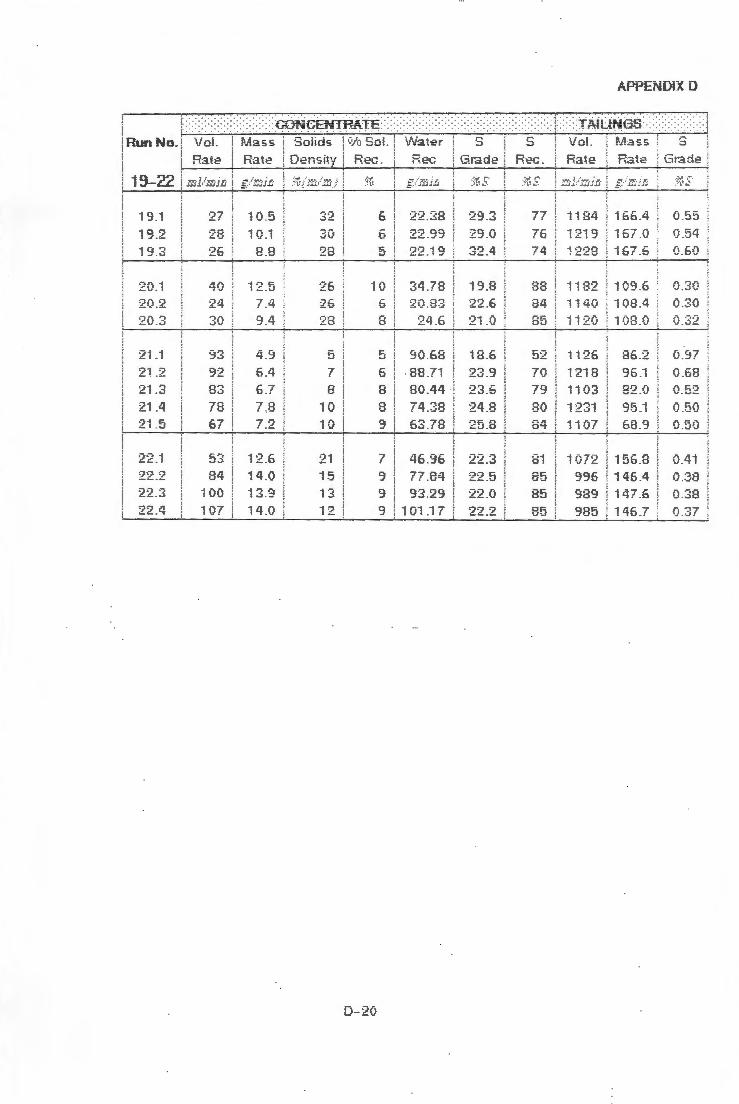
Run No_ Voi.

Rate

19.1 27

19 .2 28 19.3 26

20.3 30

2i .i 93 21 .2 92 21 .3 83 21 .4 78

22 .i

22 .3

22.4

53

100

107

Mass l Solids O/o Sol. Water S S i

Rate j Ciensity ReG. Rec Gracie Rec.

i0 .5

10.1 r , r , c . c

i 2 .5 7.4

9.4

4 .9

6.4

6 .7 7 )3

i 2 .6 14 .0 i 3 .9 14.0

32 30 28

.-.r ~o

28

5 7 8

10 iO

2i 15 i ~. ,,:;

f,

6

5

10

D-20

f.

8

5 6

8

8 9

7 9 9

'3

22 .38

22 .93 22 .19

34.78 20 .83

24.6

90 .68 -88 .71

74.38 ,-,-. -,.:-. o,:; .: o

46.96 77 .84 93 .29

101 .17

:29 .3

:23.0

32.4

i9 .8 22.6 21.0

18.6

23 .'3 23.6

24 .8 25 .8

22 .3 22.5 :22 .0

22 .2

77

76 74

88 84 85

52

70 79 80 84

8i

85 85

APPENDIX 0

........ .... : i:AiUNGS: : . . . ...

Vo!. fl.,fass S

Rate Rate Grade

1 i !=l.'1 166.4

1219 167.0 1228 167 .6

ii 82 109.6 1140 108.4 ii2'J 108.0

11 :26 86 .2

1218 96 .1 1103 82 .{J

1231 95 .1 ii07 68.'3

i 072

989 985

156.8 145 .4 147 .6

146.7

0 .55

0.54 0 .60

0 .30 0 .30

0.32

0 .97

0 .68 0.52

0.50 0 .50

0.41 0 .38 0 .38

0 .37

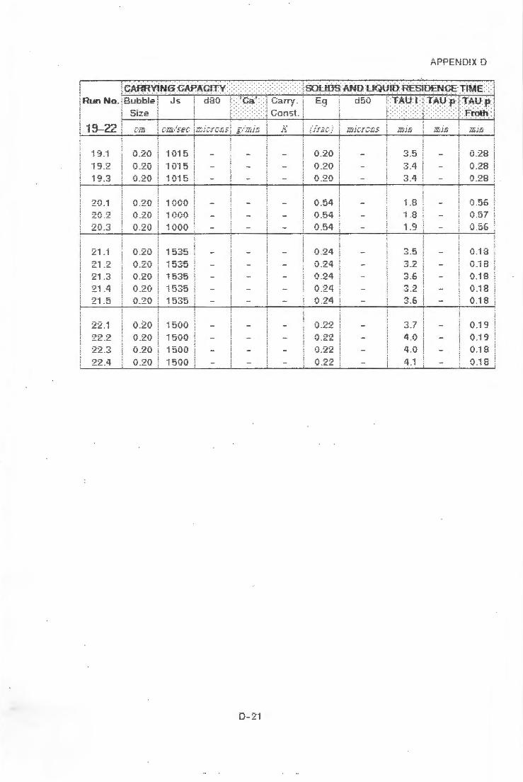
Run No_ Bubble i J ~ d80

19-22

19.1

19.2 19.3

20.1 20 .2 20.3

:2i .1

21 .2 21 .3 21.4 21 .5

22 .2 .-. .-.. -. .LL . .:J

22 .4

l Size i

0 .:20

0 .2f>

0 .20

0 .20 0.20

0 .:20

0.20 0 .20

0.20

0 .:20 0 .20

1015

11Jl 5 1 Oi 5

1000 1000 iOOO

1535

1535 1535

i 500 1500 1500

1500

D-2i

0.20

tJ.~tJ

0 .20

0 .54 0.54

0 .:24

0 .24 <j_24

0.24 0.24

0.22 0.22 i} . :2:2

0 .22

3 .5

3 .4

• r. : . 0

-j 0 ! . ...:

; .-. l . :J

3.5

r, r .> . O

3.2 3.6

·: , 7 v .,

4 .0 4 .0

4 .1

APPENDIX D

0 .:28

0 .28 0.28

0.56 0 .5? 0.56

0.18

0 .18 0 .18

0.18 O.iB

O.i '3 0 .19 O.if!

0 .18

APPENDIX E

PARTICLE SIZE DATA

The particle size data is recorded as a weight percent in each

size fraction. There are however exceptions when the particle

size data is recorded in terms of mass of solids collected in

the concentrate.

The tables that use the mass collected instead of the weight

percent in each size fraction are marked with a MC <g) . The MC

(g) stands for mass of solids, in gramms, collected per

minute.

E-1

APPENDIX E

I COMPARISON BETWEEN COLUMN .AND CONVENTIONAL BATCH CELL r·· ··r ··is·-· .·. :-:-:~ :-: -:• : : : : : CONVtNTJ:ONAl: :a:AT:CH: ft;;OTA:l:l(JN::::::::::: I:: 8lJ#. :~ -O ::: f:: :: :: : :: : : ::: :::>: j i (MiGronsj Con,~ :J ! Conc4 ! Conc5 ! Conc6 ! Column ! : l I i l I

i 1.2 0 .0 I o.o I 0.0 I 0 .0 I 0 .0

I I I j I I I j 1 .5 0 .0 I 0 .0 I 0 .0 0 .0 I 0.0 I

I I I I I I i 1.9 0.0 0 .0 0 .0 0 .0 I 0 .0 I i I

I 2.4 0 .3 Q? I 0.1 I 0 .3

I 0 .0 I _....,

I I 3 .0 2 .0 I 1.9 1 .8 j

2 .8 0.3 I

I I I I I 3 .9 1 .3 1 .1 1 .5 1.8 i 0 .8 I j

I I

I I i i

5.0 2 .2

I 2 .2 ! 2 .3 2.7 I 1.6 I i

! 6 .4 4 .0 4n I 3 .9 5.7 I 2.5 I I I .c.. I I l I I 8 .2 4 .9 I 4 .6 5 .3 I 7 .4 3 .1 I I i j I I I I I I 10 .5 6 .2 j 6 .0 7 .0 7.7 4 .0 i 13.6 7 .8 i 8.8 I 8.6 10.9 I 6.0 I I i i

I I I

I I !

I 17.7 8 .8 I 8 .6 10 .1 I 12.1 I 7 .9 I I i I 23.7 14.4 14.1 15.5 14.6 10.4 i I I I I ! 33.7 13.1 I 14.0 I 13.6 I 13.1 i 14.2

i I I i

I 54.9 22.2 I 20.9 I 20.5 I 14.6 27.2 !

I 118.4 12.9 i 13.4 I I I 22.0 I i I 9.7 i 6 .2 ;

I VARYING AIR RATE MEN USING THE SGDS - RUN 11 j f ::::m~:::::: ::::::::: ::::::A1~:RA:r:E:cotjlt.$~¢>) :::::::::::::::::::::::::::::::::::::::::::::::::::::::::::::::::::::~c:cro: ::::1 i {MiGrons-j 0 .87 I 1.11 I 1.58 I 2.18 2.76 ! II 2 .4 0 .005 I 0 .010 I 0 .011 I 0.032 '1 0.044 '1 I

3.o 0 .015 1 0.026 I 0.021 0 .064 o .oa1 I I 3.8 0 .060 I 0 .072 I 0 .071 i 0.166 1· 0 .191 I

I

I 4.8 0 .090 ! 0 .114 , 0.104

1

, 0 .236 0 .287 i 6.2 0.11 o I 0.139 1 0.131 0 .274 1 0 .338

1

1

7 .9 0 .184 1· 0 .217 I 0 .213 I 0 .420 . 0.493

I 10.1 0 .284 . 0 .336 ! 0 .3051 0

0 .. 56

96

92

1

1

0 .662 I

· 13.o o .354 I o .423 I o.3a7 o.736 I 1

1

.

I 16.7 0.478 I 0.516 I 0 .464 ! 0.719 0.758 !

1 21 .5 0.628 I 0 .645 i 0 .600 I 0 .840 0 .868 j

II 28.1 0.658 1 0.713 I 0 .638 0.796 0 .890 I

37 .6 0.737 I o .656 o .682 I 00

_.~91

46 11

0.787 !'.

53.5 0 .693 0 .645 0.758 i ., 0 .633

I 87.2 0 .583 I 0 .558 0.7471 0 .293 I 0.478

I 188.0 0 .095 i 0.083 I 0.305 0.019 1 0 .051 I 1 I I I I i

E-2

APPENDIX E

!VARYING AIR RATE Wt-EN USING TIE FCS - RUN12 F::: ::si::n.r :: :: ::::::::::::: :: :AJ:Rf~AJg:{(im/$~}:::::::>:::::::::::::::::::::::::::::::::::::::::::::::::::::::: NC: -: :::1 i (M~rons}

I 1 .2 i 1.5

I 1.9 ! 2.4 ! I I

I I ! i I

I I

I

3 .0 3.9 5.0 6.4 8 .2

10.5 13.6 17.7 23.7 33.7 54 .9

I 11e.4

2.5 0.000 I

I 0 .000 I

0.000 '1'

0.000 I

0.006 I 0 .025 1 0.075

0 .157 1 0 .208

0.25a I o.447 1

0 .629 i 0.730 I 0 .944 1 1 .591 i 1 2 ,:,,:, ! . ...,...,

0 .000

0.000

0.000 I 0.000

0 .009 1 0.047 j 0.142 i 0 .256 I 0.294 I o .465 I 0.731 1'

0 .845 1 .329 1 .509 2.354 1 .509

3.5 0 .000 I 0.000 i 0.000 I 0 .000 I 0 .022 I 0.076 j 0 .174 1 0 .316 I

o .392 I o .523 I 0 .849 1

1 .089 1 1 .448

1.786 '1

2.581 . 1 .623

4.o I

~ :~~~ I i 0 .000 I

0 .000 i 0 .025 j o.os1 I 0 .175 1

1

0.312

0.399 1 0.599 j

0 .023 I 1 .085 1· 1.484 1.846 l 2 .955 ! 2.756

!VARYING AIR RATE Wt-EN USING TIE USBM - RUN13

4.5

0 .000 I 0.000 I

0.000 0 .014

0 .069 I 0 .137 I 0 .137 o .411 1 0 .521 0.672

1 .056 I 1 .302

1 .631 I 2 .125 2 .948 2.577

5 .7 0.000 ! 0 .000 I

I 0 .000 I 0 .065 1

0.341 I 0.243

0 .341 I 0 .665 1 o .892 I 0 .892 I 1.135 I

1 .395 1.849

1 .817 I

3 .341 I 3 .212

f:::: ~J:l~:::::. :::::::::::::::::A~:RA:TI;:«:w.~~r::::::::::::::::::::::::::::::::::::::::::::::::::::::::::::::::::~c:f -: -:-1 i {A1icron45) 1.51 1.1 .. 11 0 .60 2 .33

1 .2 0 .000 0.000 I 0.000 I 0.000

1.5 0 .000 0 .000 0.000 1· 0 .000 1 .9 0.000 0.000 0 .000 0.000

2.4 0 .000 0 .000 0 .000 I 0 .000 3.0 0 .004 1 0 .000 0 .000 0.026 I 3.9 0.024 I 0.014 I 0 .017 I 0 .062 I 5 .9 0 .073 0.054 0 .075 i 0.113 I 6.4 0 .138 0 .107 0.104 0 .185 1 8 .2 0 .163 0 .140 0.120 0 .231

10.5 13.6 17.7 23.7

54 .9 118.4

0.216 0.330 0.395

o.496 I 0.716 I 1 .013 0.496

0 .186 0.275 0 .343 0.461 0 .594 0.884 0 .515

0.262 0.307 0 .303 0.661 0.590 1.101 0 .615 I

E-3

0 .293 0 .405 0.498

0 .662 1 0 .832 1 1.196 o .636 I

APPENDIX E

iVARYING THE FROTH DEPTH - RUN15 I I · · ·si:zs· · · ~. ... . . . ... .. ·.·. . .·.· .· :: : :: : ::: : : :: ::: fR<-rTH :o®H: {c~ }::::: :: : : :: : : : : : : : : :: : : : : :: : : ::: ::: : : : :: : : : : •:••: :: :: : : : : : : : : : : : : : : : : : •::::: :• ::: •:1 i (lifi,:;ronsj 1<,'t(,l l 75 ! 5(} 25 I i I i I 1.9 0 .0 I 0 .0 l 0 .0

I 0 .0 ! I I

! I I I i

I 2 .4 0 .0 I 0 .0 I 0 .1 0.1 I l 3 .0 0 .2 0 .3 0 .3 ! 0 .4 i ! i

I I i

I I 3 .8 2.0 I 2 .0 I 2.1 2 .1 I i

4.8 "' -:, 2 .8 I 2 .5 2.6 I I .>.- I i I I 6 .2 1 .9 ! 1.8

I 1.7 1 .9 I I

I I I

i 7 .9 3.4 3.1 3.1 3.3

I !

I I 10.1 5.7 5 .3 4 .8 I 5 .2 I I

I 13.0 7.4 i 6.5 6 .2 6 .8 i

I I I i 16.7 9 .1 7.9 I 7 .9 I 8 .8 I I

I 21.5 11 .0 I 10.2 9 .4 9 .8 I I I I I I

28.1 12.0 i 11 .4 I 10.5 I 10.9 l I I I I

I I 37.6 14.6 13.9 14.0 I

14.5 I I I I I I I 53.5 10.8 I 13.0 11 .4 I 10.6 I I I I I I

87.2 11.8 I 15.0 15.6 I 14.1 ! I I 188.0 6 .6 I 6.7 I 9 .0 l i

i I 10 .5 I I i I

1VARYING THE PERCENT SOLIDS FEED RATE RUN16 I - i

k: :S~-U~::: > :::: :::::: ::~ .:~L~O~F:gEo:~r•,J:Sl:f:~(:frn~~$t-rn~~$} :::: :::: :::::::::::: :::::::: ::~o:cq}: ::• i I (f.ifiGrons} 8 .,7 I 15.9 25.3 I 38.4 I ! i i i I 1.2

~.~~~ I 0 .000 I 0.000 I 0 .000 ! I f

I I 0 .024 1

I I I 2.4 0.008 I 0 .011 I I I i 3.0 0 .021 0 .034 1 0 .055 0.084 I I I

I 3 .8 0 .121 . 0 .202 1 0 .262 0 .240 I

I

I

I 4 .8 0.156 I 0.327 0.372 1 i 0.269 1 I 6 .2 0.114 I 0 .251 0 .552 !

I 0 .168 I

o .ao4 I I I 7 .9 o.185 I 0.269 0.403 I i

10.1 I 0 .479 0 .632 0 .876 1 I I I 0.298 I I I 13.0 0 .383 . 0.588 0.114 I 1 .224 i I I I I I

16.7 0 .504 0.655 i 0 .926 I 1.728 1

I I

I 21.5 0.653 1 0 .8991 1.123 1 1.848 !

I I

28.1 0.160 I 0 .991 I 1.243 I 1 .608 I I f I I

I 37 .6 1.037 I 1.168 I 1 .439 j 1 .224 ! I l

0 .9831 1 .210 I 0.192 I I I 53 .5 0 .937 I I

I i

I I i 87.2 1.1931 1.109 I 1 .362 I 0.480 I 188.0 0.731 0.168 !

I 0.571 i 0 .850 i j

E-4

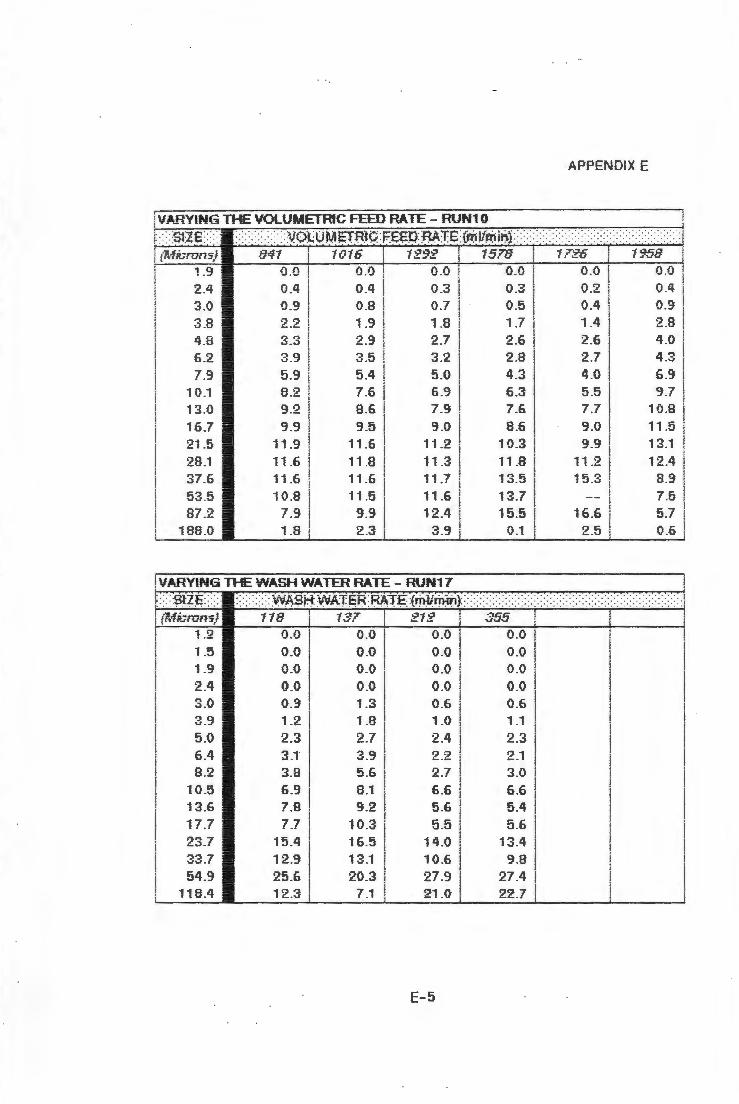
APPENDIX E

V,'_f=?YING THE VOLUMETRIC FEED RATE - RUN10

::;:'.SllS::::: ::::::::: ::: ::: :VO.lUMeT:fUO. :FBED:RATE :rtiil/r.nihj :::::::: ::::::::::::: ::::::::::::::::::::::: ::::: :::: j ...... . ............ .. ....... ·~ ................ . .............

j (f.-ff,.;rons} 841 1016 1292 i 1578 i 1l'26 1958 1.9 0 .0 I 0 .0 i 0 .0

I 0.0 I 0 .0

I 0 .0

i I I 2.4 o_q I 0 .4 0 .3 0 .3 I 0 .2 0 .4

3.0 0.9 I 0.8 I 0.7 I 0 .5 0.4 i 0.9 I I I 3.8 2.2 j 1 .9

I

1 .8 1.7 1.4 I 2 .8 I i 4 .8 ~-"' I 2 .9 2.7 2 .6 2 .6 4 .0 .:> • .:) ! I I

6 .2 3 .9 I 3.5 3.2 2 .8 I 2.7 4 .3

I I 7.9 5.9 I 5 .4 I 5 .0 4 .3 i 4 .0 6 .9

i I I I 10.1 8 .2 7.6 6 .9 I - '3 5 .5 9.7 I

I

I D .u I

13.0 9 .2 i 8 .6 7.9 I 7 .6

I 7.7 10.8

I j 16.7 9.9 I 9 .5 9.0

I 8 .6 9.0 11 .5

21.5 11.9 I 11.6 11 .2 10.3 9 .9 13.1 I I

28 .1 11 .6 I 11 .8

I 11 .3

I 11.8 i 11 .2 12.4

37.6 11 .6 11.6 11.7 13.5 I 15.3 8 .9 I I I I 53 .5 10.8 ! 11 .5 11 .6 I 13.7 I -- I 7 .5

I I I I 87 .2 7.9 I 9 .9 12.4 ! 15.5 16.6 l 5.7

188.0 1.8 ! 9 '3 ! 3 .9 ! 0.1 2 .5 0 .6 ~ .u

: VARYING THE WASH WATER RA TE - RUN17 ~:: ::£~~:::::: :::::: ::::: :w.ASH.WA:T:~~:RAT~ :(~m.o:i}:::::::::::::::::::::::::::::::::::::::::::::::::::::::::::::::::::::: (l:.,fi,.;rons} 118 137 212 355

1 .2 0 .0 I 0 .0 I 1 .5 o.o ,. o.o I 1.9 o.o o.o l 2 .4 o.o I o.o , 3 .o o .9 j 1.3 I 3 .9 1 .2 I 1 .8 1· 5 .o 2.3 I 2.7

6.4 3 .1" 1 3 .9 I 8 .2 3 .8 I 58 .. 16 1

10.5 6 .9 I 13.6 7 .8 I 17.7 7.7 1 23.7 33.7 54 .9

118.4

15.4 I 12.9 I 25.6 I

1 n '3 ! c...u

9 .2 10.3 16.5

13.1 I 20.3 I

7 .1

0 .0 0.0 0 .0 0 .0 l o.o I o.o I 0 .0 o.o I o .6 I 0 .6 1 .0 I 1 .1 i 2.4 I 2.3 j 92 1 2.1 I ; :1 I I

3 .o I 6 .6 I 6 .6 I

5 .6 I 5.4 I 5 .5 5 .6

14.0 13.4 10.6 9 .8 27.9 I 27 .4 21 .0 I 22.7 I

E-5

! I I ! I

I I I I

I I I I I

I I

i I ! i

APPENDIX E

! VARYJNG 11-E WASH WATER POSITION - RUN18 I

r::::s~-zs:::::- :: :: : : : : : : : : : : : : WASH: WATlER :ro.stTION '.(¢m}: :: : : : : :: :: : :: : : :: : : : : : : : : : : : : : : : : :: : :: : : : : : : : : : : : : : : :: : : :::: :: I {Micron'5} 5 10 ! 15 ;?() I :

I 1.9 0 .0 ! 0 .0 ! 0 .0

I o.o I I

I 0 .0 l I I I 2 .4 0 .0 0 .0 o.o I I o.o I o.o I I

I 3 .0 0 .0 0 .1 I

l 3.8 0 .4 I 0 .5 I 0 .5 0 .5

I 4.8 0 .9 I 0.9 0 .9 j I 0 .9 I

I I 6 .2 1 .1 I 1 .0 I 1 .0 1 .0

I I i 7.9 1.7 I 1 .6 1.6 I 1 .6 l I 10.1 I 2.7 2.6 I 2.5 2.7 I

I I 13.0 3 .8 j 3.7 3 .7 3.6 I I I

I 16.7 5.4 j 5 .4 I 5 .4

I 5 .2

I 21.5 1.a I 7.7 I 7.5 7.3 I I I I 28 .1 9.8 I 9 .0 I 9 .8 I 9 .5

I I I I 37 .6 13.6 13.6 1 13.6 13.2 53.5 15.3 I 15.3 I 15.2 15.1 I I I

I 87.7 20.5 21 .0 I 21 .1 21 .3 I

188.0 16.8 16.7 17.1 10.2 I I

!VARYING TI-E WASH WATER TEMPERATURE - RUN7 f. ·mzE .. <<· .. . .. <·> :;:::;:;:::WA~H:WAT:~R:ra;1~eRA:W.~{O~gr~~:G~~~}::::::::::::::::::::::::::::: j {1Aicron'5} 21 I 3{) 40 5()

I 1 .2 0 .0 I 0 .0 I 0 .0 0.0 I I 2 .4 0 .4

I 0 .3 I 0 .3 0 .3 I I ! I

I 3.0 0.7 ! 0.7 I 0 .6 0 .6

I I i I ! 3 .8 , .9 I 1 .9 I 2 .1 2 .2

I I 4.8 3 .0 I 2 .8 3 .1 ... ..,, I

,> . ,> I 6 .2 ?? I ":.'? 3 .2 I ?? I ..., _..., ..., _..., ..., __

7 .9 5 .2 I 5 .2 I 5.1

I 5.2 I

10.1 7 .5 7 .5 I 7 .9 7.7 I I 13.0 8 .6 I 8 .4 9 .2 I 9 .1 I I I 16.7 9 .5 I 9 .6

I 10.3 I 10.2

I i I 21.5 10.9 I 11 .6 12.9 12.2 i I I I

I I

28.1 11.7 I 12.1 I 13.4 I 1 2 .2 I 37.6 12.7 12.4

I 12.3 I 12 .7

I

I i ! i 53.5 11.4 ! 12.5 10.5 i ,o .3 I

! 87 .2 12.6 I 11.1 i

8 .3 I

I I 9.9 I I I 188.0 0.1 I o .6 I 0 .8 I 0.4 1 I

E-6

APPENDIX E

jVARYING THE COLLECTOR DOSAGE RATE - RUN21 ··:::::Sl'.ze::> : : : : : : : : : : : : : : : : :w.LJi.;£rC.1Q:fl :PQSA~8 :RAT€: {tift{)~}::::::::::::::::::: ::::::::::::::::::::::::::::::::: i 1 {1.1icronsj 9.8 21] 4,;,,;, -·- 6f)] 121 .5

! 1.2 0 .0 i 0 .0 I 0 .0 I 0 .0 I 0 .0

I i

i 1 .5 0.0

I

0 .0 i 0.0 I 0.0 i 0 .0

I 1 .9 0 .0 0 .0 I 0.0 I 0 .0 I 0.0 I I i I

I 2.4 0 .0 0 .1 I 0 .0 0.0 I 0 .0

I I 3 .0 0.3 0.5 I

0 .3 I

0 .0 i 0 .0 I i I I i 3 .9 0 .9 I 0 .9 I 0 .6 I 0.2 0.2 i i I I I ! 5 .0 2.7 2.0 I 1.8 i 1.2 I 1 .3 I i 6 .4 1 .5 I 1 .4 1 .1 I 0 .5 I 0 .5 I i

I i I i

I I 8 .2 2 .1 2.1 i 1.5 I 0.8 i 0 .7 i I I i 10 .5 7 .1 I 6 .2 5 .3 I 4 .0 I 3.6

I I I

I .. "'r 6 .3 i 5 .5 4.9 I 2.7 I 2 .9 I

1 .:, . 0 I

I 17.7 6 .2 i 5 .9 I 4 .9 I 3 .0 ! 2 .6 I I I I

I 23.7 16.9 i 15.7 I 14.0 I 11 .5 I 3 .8 I 33.7 12.1 I 11 .6 I 11 .2 I 10.1 I 9.4

! I I i I I 54 .9 25.2 i 26.4 I 26.4 i 30.9 27.6

I 118.4 18.6 I 21.7 i 28 .1 I 35.0 i 41 .3 I I I

I

k::::::::::;:;::: : :::;:::::::::;:::::::::::::;:;:::::::::::::::::::::::::;:;:;:::::::::::::::;:;:;:::::::::::::::;:'.:;::::::<:;:::::;::: ::::::;:;:;:'.:; ::: :::i

I I I 1 ·

i I I I I I

E-7

APPENDIX F

PILOT PL.ABT DATA

The data recorded for the pilot plant test work together with

the calculated data is given in this appendix .

The fractional gas holdup was estimated by stopping the feed

and tailings pumps, as well as the air to the column. The

fractional gas holdup could only be estimated due to the pulp

from the froth increasing the reading for the pulp in the

collection zone .

The mean liquid residence time was calculated by assuming that

the liquid flow was plug flow.

F-1

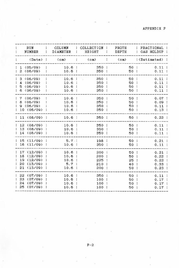
RUN NUMBER

<Date)

1 (05/09) : 2 (06/09)

3 (06/09) 4 (06/09) 5 (06/09) 6 (06/09)

7 ( 06/09) 8 (06/09) 9 (06/09) 10 (06/09)

11 (08/09)

12 (08/09) 13 (08/09) 14 (08/09)

15 (11/09) 16 (11/09)

COLUMN DIAMETER

: COLLECTION:

(cm)

10.6 : 10.6 :

10.6 10.6 10.6 10.6

10 . 6 10.6 10.6 10.6

10.6 :

10.6 10.6 : 10 . 6 :

5.7 I I

10.6 I I

HEIGHT

(cm)

350 : 350 :

350 350 350 350

350 350 350 350

350 :

350 350 : 350 :

198 I I

350 I I

FROTH DEPTH

(cm)

APPENDIX F

: FRACTIONAL : : GAS HOLDUP :

: <Estimated)

50 : 50 :

50 50 50 50

50 50 50 50

50 :

50 50 : 50 :

50 I I

50 I I

0.11 : 0.11 :

0.11 0.11 0.11 0.11

0.07 0.09 0.11 0.13

0.22 :

0.11 0. 11 : 0 . 11 :

0.21 I I

0. 11 I I

- --------------------------------------- --------------------------17 (12/09) 10.6 200 50 0.21 18 (12/09) 10.6 200 50 0.22 19 (12/09) 10.6 225 25 0.22 20 (13/09) 5.7 210 40 0.33 21 (13/09) 10.6 200 50 0.23

------------------------------------------------------------------22 (07/09) 10.6 350 50 0.11 23 (07/09) 10.6 100 50 0.17 24 (07/09) 10.6 100 50 0.17 25 (07/09) 10.6 100 50 0. 17

F-2

APPENDIX F

- - ----------------------------------------------------------------RUN

NUMBER AIR RATE

WASH WATER : RATE

FEED RATE

TAILINGS RATE

------------------------------------------------------------------

1 2

3 4 5 6

7 8 9 10

11

12 13 14

15 16

17 18 19 20 21

22 23 24 25

<ml/min)

11650 : 11650

11650 11650 11650 11650

7714 9906

11650 12857

12030 :

11650 11650 11650

3445 : 11650

17352 20773 20773

5714 24127

11650 11650 11650 11650

(ml/min)

941 761

F-3

0 414 941

1462

941 941 941 941

941

0 64 :

1181

277 941

1462 1462 1462

277 1462

941 941 941 941

(ml/min)

3660 :

3919 4160 3900 4621

4252 4133 3900 3822

2704

2952 3194 2607

521 3227

1346 1299

999 1703 1082

2902 2916 3301 4086

<ml/min)

4197 :

3884 4514 4748 5860

5150 5020 4748 4645

3498 :

2590 2904 : 3409 :

742 ! 3903

2514 1866 1436 1926 1703

3697 3783 4162 4907

RUN NUMBER

1 2

3 4 5 6

7 8 9 10

11

12 13 14

15 16

17 18 19 20 21

22 23 24 25

APPENDIX F

:CONCENTRATE: FEED :CONCENTRATE: TAILINGS RATE :SOLIDS RATE :SOLIDS RATE :SOLIDS RATE:

(ml/min)

224

35 60 93

223

43 53 93

118

147

362 354 379

56 265

294 894

1025 54

841

146 73 80

120

(g/min)

F-4

1882

2223 2271 2175 2625

2361 2244 2175 2154

1126

851 535 953

227 1822

569 577 593 448 466

1472 1292 1713 2080

(g/min)

10

9 12 15 15

10 11 15 14

6

72 60 27

7 19

9 20 22

2 17

11 6 9

13

(g/min)

1872

2214 2259 2161 2610

2351 2233 2161 2140

1120

779 474 926

220 1803

559 557 571 447 448

1461 1286 1704 2067

APPENDIX F

------------------------------------------------------------------RUN

NUMBER :SUPERFICIAL

AIR RATE :SUPERFICIAL :SUPERFICIAL :W/WATER RATE: BIAS RATE

:MEAN LIQUID : :RESIDENCE t

------------------------------------------------------------------

1 2

3 4 5 6

7 8 9 10

11

12 13 14

15 16

17 18 19 20 21

22 23 24 25

(cm/sec)

1. 84

1. 84 1. 85 1. 86 1.86

1. 22 1.58 1. 86 2.06

1. 97

1. 88 1. 83 1. 88

2.07 1. 83

3.02 3.60 3.57 3.42 4.19

1. 85 1. 88 1. 87 1. 86

(cm/sec)

F-5

0.14

0.00 0.08 0.18 0.28

o. 18 0.18 0.18 0.18

0.18

0.00 0.01 0.22

0. 18 0.18

0.28 0.28 0.28 0.18 0.28

0.18 0.18 0.18 0.18

(cm/sec)

0.10

-0.01 0.07 0 . 16 0.23

0.17 0.17 0.16 0.16

0.15

-0.07 -0.05

0.15

0. 14 0.13

0.22 0.11 0.08 0.15 0.12

0.15 0.16 o. 16 o. 16

(min)

6.55

7.08 6.09 5.79 4.69

5.58 5.60 5.79 5.79

6.89

10.61 9.47 8.06

5.38 7 . 04

5.55 7.38

10.78 1. 86 7.98

7.44 1. 94 1. 76 1. 49

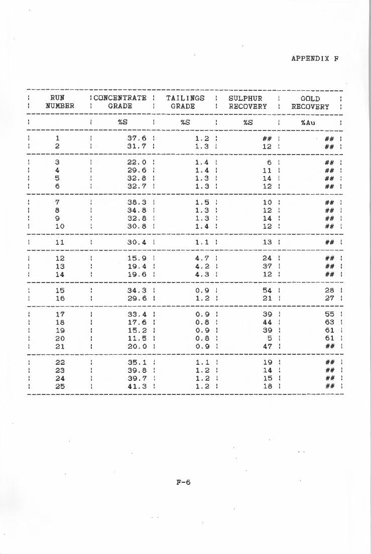
APPENDIX F

------------------------------------------------------------------RUN

NUMBER :CONCENTRATE

GRADE TAILINGS

GRADE SULPHUR RECOVERY

GOLD RECOVERY

------------------------------------------------------------------

1 2

3 4 5 6

7 8 9 10

11

12 13 14

15 16

17 18 19 20 21

22 23 24 25

%S

37.6 31. 7

22.0 29.6 32.8 32.7

38.3 34.8 32.8 30.8

30.4

15.9 19.4 19 . 6

34.3 29.6

33.4 17.6 15.2 11. 5 20.0

35.1 39.8 39.7 41. 3

%S

F-6

1. 2 1. 3

1. 4 1. 4 1. 3 1. 3

1. 5 1. 3 1. 3 1. 4

1. 1

4.7 4.2 4.3

0.9 1. 2

0.9 0.8 0.9 0.8 0.9

1. 1 1. 2 1. 2 1. 2

%S

## 12

6 11 14 12

10 12 14 12

13

24 37 12

54 21

39 44 39

5 47

19 14 15 18

%Au

## ##

## ## ## ##

## ## ## ##

##

## ## ##

28 27

55 63 61 61 ##

## ## ## ##

RUN NUMBER

1 2

3 4 5 6

7 8 9 10

11

12 13 14

15 16

17 18 19 20 21

22 23 24 25

FEED GRADE

PERCENTAGE : : SOLIDS REC :

%8

## : 1.46

1. 51 1. 50 1. 54 1.51

1. 65 1. 43 1. 54 1. 62

1. 28

5.63 5 . 92 4 . 75

1. 85 1. 45

1. 42 1. 38 1. 44 0.87 1. 58

1.35 1. 37 1. 41 1. 46

%

## : 0.53

0.40 0 . 53 0.67 0.57

0.44 0.49 0.67 0 . 65

0.53

8.41 11. 30 2.86

2.93 1. 03

1.66 3 . 50 3.69 0 . 38 3.74

0.75 0.50 0.52 0.62

F-7

% SOLIDS IN CONC.

%

APPENDIX F

: SUPERFICIAL : :BUB. SURFACE:

Js

## : ## : 4 . 34

21. 72 17.76 14.28 6.39

21 . 03 18.31 14.28 11.03

3 . 97

17 . 59 15.41 6.88

10 . 97 6.78

3.15 2 . 23 2.11 3 . 09 2.04

7.18 8 . 31

10.52 10.12

961. 82 :

961. 82 966 . 64 969.84 970 . 51

6 3 7 . 92 822 . 50 969.84

1073.45

1029.27

980 . 78 952.38 : 982 . 96 :

1079.42 : 956.11

1573 . 50 1877 . 06 1864.39 1784 . 63 2187.07

964 . 77 981. 00 973 . 08 971.62

the determination of the effects of physical and chemical

Documents