the diagonal of the stasheï¬€ polytope

The diagonal of the Stasheff polytope

Jean-Louis Loday

Institut de Recherche Mathematique AvanceeCNRS et Universite Louis Pasteur7 rue R. Descartes67084 Strasbourg Cedex, [email protected]

To Murray Gerstenhaber and Jim Stasheff

Summary. We construct an A-infinity structure on the tensor product of two A-infinity algebras by using the simplicial decomposition of the Stasheff polytope.The key point is the construction of an operad AA-infinity based on the simplicialStasheff polytope. The operad AA-infinity admits a coassociative diagonal and theoperad A-infinity is a retract by deformation of it. We compare these constructionswith analogous constructions due to Saneblidze-Umble and Markl-Shnider based onthe Boardman-Vogt cubical decomposition of the Stasheff polytope.

Key words: Stasheff polytope, associahedron, operad, bar-cobar construction, co-bar construction, A-infinity algebra, AA-infinity algebra, diagonal.2010 Mathematics Subject Classification. 18D50, 55U35, 52B11

Introduction

An associative algebra up to homotopy, or A∞-algebra, is a chain complex(A, dA) equipped with an n-ary operation µn for each n ≥ 2 verifying µµ = 0.See [15], or, for instance, [5]. Here we put

µ := dA + µ2 + µ3 + · · · : T (A) → T (A),

where µn has been extended to the tensor coalgebra T (A) by coderivation. Inparticular µ2 is not associative, but only associative up to homotopy in thefollowing sense:

µ2 (µ2 ⊗ id) − µ2 (id ⊗ µ2) = dA µ3 + µ3 dA⊗3 .

Putting an A∞-algebra structure on the tensor product of two A∞-algebrasis a long standing problem, cf. for instance [12, 2]. Recently a solution has

2 Jean-Louis Loday

been constructed by Saneblidze and Umble, cf. [13, 14], by providing a diag-onal A∞ → A∞ ⊗ A∞ on the operad A∞ which governs the A∞-algebras.Recall that, over a field, the operad A∞ is the minimal model of the operadAs governing the associative algebras. The differential graded module (A∞)n

of the n-ary operations is the chain complex of the Stasheff polytope. Themethod of Saneblidze and Umble consists in providing an explicit (i.e. combi-natorial) diagonal of the Stasheff polytope considered as a cellular complex. In[11] Markl and Shnider give a construction of the Saneblidze-Umble diagonalby using the Boardman-Vogt model of As. This model is the bar-cobar con-struction on As, denoted ΩBAs, in the operadic framework. It turns out thatthere exists a coassociative diagonal on ΩBAs, which is constructed out ofthe diagonal of the cube. This diagonal, together with the quasi-isomorphismsq : A∞→ΩBAs and p : ΩBAs→A∞ permit them to construct a diagonal onA∞ by composition:

A∞q→ ΩBAs → ΩBAs ⊗ ΩBAs

p⊗p−→ A∞ ⊗ A∞ .

The aim of this paper is to give an alternative solution to the diagonalproblem by relying on the simplicial decomposition of the Stasheff polytope

described in [8] and using the diagonal of the standard simplex. It leads toa new model AA∞ of the operad As, whose dg module (AA∞)n is the chaincomplex of a simplicial decomposition of the Stasheff polytope. Because of itssimplicial nature, the operad AA∞ has a coassociative diagonal (by meansof the Alexander-Whitney map) and therefore we get a diagonal on A∞ bycomposition:

A∞q′

→ AA∞ → AA∞ ⊗ AA∞p′⊗p′

−→ A∞ ⊗ A∞ .

The map q′ : A∞ → AA∞ is induced by the simplicial decompositionof the associahedron. The map p′ : AA∞ → A∞ is slightly more involvedto construct. It is induced by the deformation of the “main simplex” of theassociahedron into the big cell of the associahedron. Here the main simplexis defined by the shortest path in the Tamari poset structure of the planarbinary trees.

We compute the diagonal map on (A∞)n up to n = 5 and we find the sameresult as the Saneblidze-Umble diagonal. So it is reasonable to conjecture thatthey coincide.

In the last part we give a similar interpretation of the map p : ΩBAs→A∞

constructed in [11] and giving rise to the Saneblidze-Umble diagonal. It isinduced by the deformation of the “main cube” into the big cell.

Acknowledgement I thank Bruno Vallette for illuminating discussions onthe algebras up to homotopy and Samson Saneblidze for sharing his drawingswith me some years ago. Thanks to Emily Burgunder, Martin Markl, Samson

The diagonal of the Stasheff polytope 3

Saneblidze, Jim Stasheff and Ron Umble for their comments on the previousversions of this paper. I warmly thank the referee for his careful reading andhis precious comments which helped me to improve this text.

This work is partially supported by the French agency ANR.

1 Stasheff polytope (associahedron)

We recall briefly the construction of the Stasheff polytope, also called associ-ahedron, and its simplicial realization, which is the key tool of this paper. Allchain complexes in this paper are made of free modules over a commutativering K (which can be Z or a field).

1.1 Planar binary trees

We denote by PBTn the set of planar binary trees having n leaves:

PBT1 := |, PBT2 := ??

, PBT3 :=

???? ,??

???? ,

PBT4 :=

::::: ,

::

::::: , ::

::::: ,:::

::::: ,

:::::

::::: .

So t ∈ PBTn has one root, n leaves, (n − 1) internal vertices, (n − 2)internal edges. Each vertex is binary (two inputs, one output). The number of

elements in PBTn+1 is known to be the Catalan number cn = (2n)!n! (n+1)! . There

is a partial order on PBTn, called the Tamari order, defined as follows. OnPBT3 it is given by

???? →??

???? .

More generally, if t and s are two planar binary trees with the same numberof leaves, there is a covering relation t → s if and only if s can be obtained

from t by replacing a local pattern like

???? by??

???? . In other words

s is obtained from t by moving a leaf or an internal edge from left to rightover a fork.

Examples:

4 Jean-Louis Loday

yyyEEE

•

1

sssKKKwwwww

GGGGGwwwww

GGGGG

//

12 21

123

xxqqqqqq

##GGGGGGGGGG

213

wwwwwwwwww 141

312&&MMMMMM

321

where the elements of PBT4 (listed above) are denoted 123, 213, 141, 312, 321,respectively. We recall from [7] how this way of indexing is obtained. Firstwe label the leaves of a tree from left to right by 0, 1, 2, . . . . Then we labelthe vertices by 1, 2, . . . by saying that the label i vertex lies in between theleaves i − 1 and i (drop a ball). To any binary tree t we associate a sequenceof integers x1x2 · · ·xn−1 as follows: xi = aibi where ai (resp. bi) is the numberof leaves on the left (resp. right) side of the ith vertex.

1.2 Shortest path and long path

The Tamari poset admits an initial element: the left comb 12 · · · (n − 1), anda terminal element: the right comb (n − 1)(n − 2) · · · 1. There is a shortest

path from the initial element to the terminal element. It is made of the treeswhich are the grafting of some left comb with a right comb. In PBTn thereare n− 1 of them. This sequence of planar binary trees will play a significantrole in the comparison of different cell realizations of the Stasheff polytope.

Example: the shortest path in PBT4:

::::: → ::

::::: →

:::::

:::::

We also define “the long path” as follows. The long path from the leftcomb to the right comb is obtained by taking a covering relation at each stepwith the following rule: the vertex which is moved is the one with the smallestlabel (among the movable vertices, of course).

Examples: n = 2

::::: →

::

::::: →:::

::::: →

:::::

:::::

n = 3

::::::: →

::

::::::: →

:::

::::::: →

:::::

::::::: →


:::::::

::::::: →

::::::::

::::::: →

::::::::::

:::::::

Observe that there are (for n ≥ 3) other paths with the same length.

1.3 Planar trees

We now consider the planar trees for which an internal vertex has one rootand k leaves, where k can be any integer greater than or equal to 2. We denoteby PTn the set of planar trees with n leaves:

PT1 := |, PT2 :=

??, PT3 :=

???? ,??

???? ,

???? ,

PT4 :=

::::: , . . . ,

::::: , . . . ,

:::::

(((( .

Each set PTn is graded according to the number of internal vertices, i.e. PTn =⋃p=n

p=1 PTn,p where PTn,p is the set of planar trees with n leaves and p internalvertices. For instance PTn,1 contains only one element which we call the n-

corolla (the last element in the above sets). It is clear that PTn,n−1 = PBTn.We order the vertices of a planar tree by using the same procedure as for

the planar binary trees.

1.4 The Stasheff polytope, alias associahedron

The associahedron is a cellular complex Kn of dimension n, first constructedby Jim Stasheff [15], which can be realized as a convex polytope whoseextremal vertices are in one-to-one correspondence with the planar binarytrees in PBTn+2. We showed in [7] that it is the convex hull of the pointsM(t) = (x1, . . . , xn+1) ∈ R

n+1, where the computation of the xi’s has beenrecalled in 1.1. The edges of the polytope are indexed by the covering relationsof the Tamari poset.

Examples:

• //wwooooo

$$JJJJJJ

JJ

zzttt

ttttt

''OOOOO

//cc

GGGGGG

gg OOO ::ttt

tt

cc

GGGGGG

///

///

//

/// //__

????

?? gg//

??

//

K0 K1 K2 K3

6 Jean-Louis Loday

Its k-cells are in one-to-one correspondence with the planar trees inPTn+2,n+1−k. For instance the 0-cells are indexed by the planar binary trees,and the top cell is indexed by the corolla.

It will prove helpful to adopt the notation Kt to denote the cell in Kn

indexed by t ∈ PTn+2. For instance, if t is the corolla, then Kt = Kn. Asa space Kt is the product of p associahedrons (or associahedra, as you like),where p is the number of internal vertices of t:

Kt = Ki1 × · · · × Kip

where ij+2 is the number of inputs of the jth internal vertex of t. For instance,

if t =

::::::: , then Kt = K1 ×K1.

The shortest path and the long path defined combinatorially in 1.1 giverise to concrete paths on the associahedron.

To the cellular complex Kn we associate its chain complex C∗(Kn). The

module of k-chains admits the set of trees PTn+2,n+1−k as a basis:

Ck(Kn) = K[PTn+2,n+1−k].

In particular C0(Kn) = K[PBTn+2] and Cn(Kn) = K tn+2 where tn+2 is the

corolla.

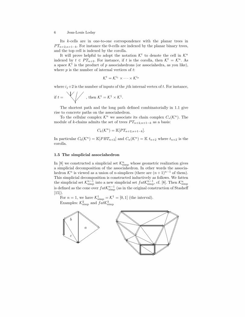
1.5 The simplicial associahedron

In [8] we constructed a simplicial set Knsimp whose geometric realization gives

a simplicial decomposition of the associahedron. In other words the associa-hedron Kn is viewed as a union of n-simplices (there are (n +1)n−1 of them).This simplicial decomposition is constructed inductively as follows. We fattenthe simplicial set Kn−1

simp into a new simplicial set fatKn−1simp, cf. [8]. Then Kn

simp

is defined as the cone over fatKn−1simp (as in the original construction of Stasheff

[15]).For n = 1, we have K1

simp = K1 = [0, 1] (the interval).

Examples: K2simp and fatK3

simp

t| pppppppp

pppppppp

'FF

FFFF

FFFF

FFFF

FFFF

FFFF

FFFF

FF

222

2222

2222

222 b

a

vvvvv

vvvv

vvvvv

''OOOOOOOOO c

+3_g

GGGGG

GGGGGGG

GGGGGGGG

GGGG

ck

OOOOOOOOOO6>

tttttt

ttt

tttttt

ttt

_g

GGGGGGG

GGGGG

GGGGGGG

GGGGG

//

////

////

/

////

////

///

+3

llYYYYYYYYYYYYY

77ooooooooooooooooo

777

7777

7777

77

JJ

''''''''''

//

///

////

/wwoooooo

''OOOOOOOOOOO[c

????

????

??

????

????

??+3

jjTTTTTTTT

$$JJJJJJJJJ

//6>

tttttt

ttt

tttttt

ttt

+3


Since, in the process of fattenization, the new cells are products of smallerdimensional associahedrons we get the following main property.

Proposition 1.6 The simplicial decomposition of a face Ki1 × · · · × Kik of

Kn is the product of the simplicializations of each component Kij .

Proof. It is immediate from the inductive procedure which constructs Kn outof Kn−1.

Considered as a cellular complex, still denoted Knsimp, the simplicialized

associahedron gives rise to a chain complex denoted C∗(Knsimp). This chain

complex is the normalized chain complex of the simplicial set. It is the quo-tient of the chain complex associated to the simplicial set, divided out by thedegenerate simplices (cf. for instance [9] Chapter VIII). A basis of C0(K

nsimp)

is given by PBTn+2 and a basis of Cn(Knsimp) is given by the (n + 1)n−1 top

simplices (in bijection with the parking functions, cf. [8]). It is zero higher up.In the sequel “a simplex of Kn

simp” always mean a nondegenerate simplexof Kn

simp.Among the top simplices there is a particular one which we call the main

simplex. Its vertices are indexed by the planar binary trees which are part ofthe shortest path constructed in 1.1 (observe that the shortest path has n+1vertices).

Examples (the main simplex is highlighted):

wwoooooooo

(JJJJJJJJJJJ

JJJJJJJJJJJ

444

4444

4444

4

v~ ttttttttttt

ttttttttttt

''OOOOOOOO

+3_g

GGGGGGGG

GGGG

GGGGGGGG

GGGG

::

ttttttttt

ggOOOOOO

cc

GGGGGGGGGGGG

///

////

////

//

llYYYYYYYYYYYYY

3;oooooooooooooooo

oooooooooooooooo

777

7777

7777

77

JJ

''''''''''fn TTTTTTTT

TTTTTTTT

bj MMMMMMMMMMMMMMMMMMM

MMMMMMMMMMMMMMMMMMM

///

///

wwoooooo

''OOOOOOOOOOO

???

????

????

//

jjTTTTTTTT

$$JJJJJJJJJ

//

//

::ttttttttt

2 The operad AA∞

We construct the operad AA∞ and we construct a diagonal on it. A morphismfrom the operad A∞ governing the associative algebras up to homotopy to theoperad AA∞ is deduced from the simplicial structure of the associahedron.

2.1 Differential graded non-symmetric operad [10]

By definition a differential graded non-symmetric operad, dgns operad forshort, is a family of chain complexes Pn = (Pn, d) equipped with chain com-plex morphisms

8 Jean-Louis Loday

γi1···in: Pn ⊗ Pi1 ⊗ · · · ⊗ Pin

→ Pi1+···+in,

which satisfy the following associativity property. Let P be the endofunctorof the category of chain complexes over K defined by P(V ) :=

⊕

n Pn ⊗V ⊗n.The maps γi1···in

give rise to a transformation of functors γ : P P → P .This transformation of functors γ is supposed to be associative. Moreover wesuppose that P0 = 0,P1 = K (trivial chain complex concentrated in degree0). The transformation of functors Id → P determined by P1 is supposed tobe a unit for γ. So we can denote by id the generator of P1. Since Pn is agraded module, P is bigraded. The integer n is called the “arity” in order todifferentiate it from the degree of the chain complex.

2.2 The fundamental example A∞

The operad A∞ is a dgns operad constructed as follows:

A∞,n := C∗(Kn−2) (chain complex of the cellular space Kn−2).

Let us denote by As¡ the family of one dimensional modules (As¡n)n≥1

generated by the corollas (unique top cells). It is easy to check that there isa natural identification of graded (by arity) modules A∞ = T (As¡), whereT (As¡) is the free ns operad over As¡. This identification is given by graftingon the leaves as follows. Given trees t, t1, . . . , tn where t has n leaves, the treeγ(t; t1, . . . , tn) is obtained by identifying the ith leaf of t with the root of ti.For instance:

γ( ??

;??

???? , ??

) =

:: ::

::::::: .

Moreover, under this identification, the composition map γ is a chain map,therefore A∞ is a dgns operad.

This construction is a particular example of the so-called “cobar construc-tion” Ω, i.e. A∞ = ΩAs¡ where As¡ is considered as the cooperad governingthe coassociative coalgebras (cf. [10]).

For any chain complex A there is a well-defined dgns operad End(A) givenby End(A)n = Hom(A⊗n, A). An A∞-algebra is nothing but a morphism ofoperads A∞ → End(A). The image of the corolla under this isomorphism isthe n-ary operation µn alluded to in the introduction.

2.3 Hadamard product of operads, operadic diagonal

Given two operads P and Q, their Hadamard product, also called tensorproduct, is the operad P⊗Q defined as (P⊗Q)n := Pn⊗Qn. The compositionmap is simply the tensor product of the two composition maps.

A diagonal on a nonsymmetric operad P is a morphism of operads∆ : P → P ⊗ P , which is compatible with the unit. Explicitly it is given by


chain complex morphisms ∆ : Pn → Pn ⊗ Pn which commute with the com-position in P . In other words, the following diagram, where m := i1 + · · ·+ in,is commutative:

Pn ⊗ Pi1 ⊗ · · ·γ //

∆⊗∆⊗···

Pm∆ // Pm ⊗ Pm

(Pn ⊗ Pn) ⊗ (Pi1 ⊗ Pi1) ⊗ · · ·∼= // (Pn ⊗ Pi1 ⊗ · · · ) ⊗ (Pn ⊗ Pi1 ⊗ · · · )

γ⊗γ

OO

We do not ask for ∆ to be coassociative.

2.4 Tensor product of A∞-algebras

It is a long-standing problem to decide if, given two A∞-algebras A and B,there is a natural A∞-structure on their tensor product A⊗B which extendsthe natural dg nonassociative algebra structure, cf. [12, 2]. It amounts toconstruct a diagonal on A∞, i.e. an operad morphism ∆ : A∞ → A∞ ⊗ A∞,since, by composition, we get an A∞-structure on A ⊗ B:

A∞ → A∞ ⊗ A∞ → End(A) ⊗ End(B) → End(A ⊗ B) .

Let us recall that the classical associative structure on the tensor product oftwo associative algebras can be interpreted operadically as follows. There is adiagonal on the operad As given by

Asn → Asn ⊗ Asn, mn 7→ mn ⊗ mn ,

where mn is the standard n-ary operation in the associative framework. Sincewe want the diagonal ∆ on A∞ to be compatible with the diagonal on As(µ2 7→ m2), there is no choice in arity 2, and we have ∆(µ2) = µ2 ⊗ µ2.Observe that these two elements are in degree 0. In arity 3, since µ3 is ofdegree 1 and µ3 ⊗ µ3 of degree 2, this last element cannot be the answer. Infact there is already a choice (parameter a) for a solution:

∆(

???? ) = a(

???? ⊗

???? +??

???? ⊗

????)

+(1 − a)(

???? ⊗??

???? +

???? ⊗

????)

.

By some tour de force Samson Saneblidze and Ron Umble constructedsuch a diagonal on A∞ in [13]. Their construction was re-interpreted in [11]by Markl and Shnider through the Boardman-Vogt construction (see section4 below for a brief account of their work). We will use the simplicialization ofthe associahedron described in [8] to give a solution to the diagonal problem.

10 Jean-Louis Loday

2.5 Construction of the operad AA∞

We define the dgns operad AA∞ as follows. The chain complex AA∞,n is thechain complex of the simplicialization of the associahedron considered as acellular complex (cf. 1.5):

AA∞,n := C∗(Kn−2simp) .

In low dimension we take AA∞,0 = 0, AA∞,1 = K id. So a basis of AA∞,n

is made of the (nondegenerate) simplices of Kn−2simp. Let us now construct the

composition map

γ = γAA∞ : AA∞,n ⊗ AA∞,i1 ⊗ · · · ⊗ AA∞,in→ AA∞,i1+···+in

.

We denote by ∆k the standard k-simplex. Let ι : ∆k Kn−2

simp be a cell,

i.e. a linear generator of Ck(Kn−2simp). Given such cells

ι0 ∈ AA∞,n, ι1 ∈ AA∞,i1 , . . . , ιn ∈ AA∞,in

we construct their image γ(ι0; ι1, . . . , ιn) ∈ AA∞,m, where m := i1 + · · · + inas follows. We denote by ki the dimension of the cell ιi.

Let tn be the n-corolla in PTn and let s := γ(tn; ti1 , . . . , tin) ∈ PTm be

the grafting of the trees ti1 , . . . , tinon the leaves of tn. As noted before this is

the composition in the operad A∞. The tree s indexes a cell Ks of the spaceKm−2, which is combinatorially homeomorphic to Kn−2×Ki1−2×· · ·×Kin−2.In other words it determines a map

s∗ : Kn−2 ×Ki1−2 × · · · × Kin−2 = Ks Km−2.

The product of the inclusions ιj , j = 0, . . . , n, defines a map

ι0 × ι1 × · · · × ιn : ∆k0 × ∆k1 × · · · × ∆kn Kn−2 ×Ki1−2 × · · · × Kin−2.

Let us recall that a product of standard simplices can be decomposed into theunion of standard simplices. These pieces are indexed by the multi-shuffles α.Example: ∆1 × ∆1 = ∆2 ∪ ∆2:

//

(2, 1)

(1, 2)

OO

//

99ttttttttttttttttt

OO

So, for any multi-shuffle α there is a map

fα : ∆l → ∆k0 × ∆k1 × · · · × ∆kn ,

where l = k0 + · · · + kn. By composition of maps we get

s∗ (ι0 × · · · × ιn) fα : ∆l → Km−2

which is a linear generator of Cl(Km−2simp ) by construction of the triangulation

of the associahedron, cf. [7]. By definition γ(ι0; ι1, . . . , ιn) is the algebraic sumof the cells s∗ (ι0 × · · · × ιn) fα over the multi-shuffles.


Proposition 2.6 The graded chain complex AA∞ and γ constructed above

define a dgns operad, denoted AA∞. The operad AA∞ is a model of the operad

As.

Proof. We need to prove associativity for γ. It is an immediate consequence ofthe associativity for the composition of trees (operadic structure of A∞) andthe associativity property for the decomposition of the product of simplicesinto simplices.

Since the associahedron is contractible, taking the homology gives a gradedlinear map C∗(K

n−2simp) → K mn, where mn is in degree 0. This map sends

any planar binary tree having n leaves to mn, and obviously induces an iso-morphism on homology. These maps assemble into a dgns operad morphismAA∞ → As. Since it is a quasi-isomorphism, AA∞ is a resolution of As, thatis a model of As in the category of dgns operads.

Proposition 2.7 The operad AA∞ admits a coassociative diagonal.

Proof. This diagonal ∆ : AA∞ → AA∞ ⊗ AA∞ is determined by its value inarity n for all n, that is a chain complex morphism

C∗(Kn−2simp) → C∗(K

n−2simp) ⊗ C∗(K

n−2simp).

This morphism is defined as the composite

C∗(Kn−2simp)

∆∗−→ C∗(Kn−2simp ×Kn−2

simp)AW−→ C∗(K

n−2simp) ⊗ C∗(K

n−2simp),

where ∆∗ is induced by the diagonal on the simplicial set, and where AW isthe Alexander-Whitney map. Observe that under the identification

C∗(Kn−2simp) ⊗ C∗(K

n−2simp) = C∗(K

n−2simp ×Kn−2

simp)

the composite morphism maps a k-simplex into a 2k-simplex. Let us recallfrom [9], Chapter VIII, the construction of the AW map. Denote by d0, . . . , dk

the face operators of the simplicial set. If x is a simplex of dimension k, thenwe define dmax(x) := dk(x). So, for instance (dmax)2(x) = dk−1dk(x). Bydefinition the AW map on Ck is given by

(x, y) 7→

k∑

i=0

(

(dmax)k−i(x), (d0)i(y)

)

.

We need to check that the diagonal is compatible with the operad struc-ture, that is, the diagram of 2.3 for P = AA∞ is commutative. First weremark that the diagonal of a product of standard simplices satisfies the fol-lowing commutativity property:

C∗(∆k × ∆l)

∆ //

∆⊗∆

C∗(∆k × ∆l) ⊗ C∗(∆

k × ∆l)

=

C∗(∆k × ∆k) ⊗ C∗(∆

l × ∆l)∼= // C∗(∆

k × ∆l × ∆k × ∆l)

12 Jean-Louis Loday

where the isomorphism ∼= involves the switching isomorphism V ⊗ V ′ ∼=V ′ ⊗ V . A similar property holds for a finite product of simplices. Startingwith a linear generator

(ι; ι1, . . . , ιn) ∈ AA∞,n ⊗ AA∞,i1 ⊗ · · · ⊗ AA∞,in

we see that ∆(γ(ι; ι1, . . . , ιn)) is made of diagonals of products of simplices.Applying the preceding result we can rewrite this element as the compositeof diagonals of simplices. Hence we get

∆(γ(ι; ι1, . . . , ιn)) = γ(∆(ι); ∆(ι1), . . . , ∆(ιn))

as expected.The coassociativity property follows from the coassociativity property of

the Alexander-Whitney map.

2.8 Comparing A∞ to AA∞

Since Knsimp is a decomposition of Kn, there is a chain complex map

q′ : C∗(Kn) → C∗(K

nsimp),

where a cell of Kn is sent to the algebraic sum of the simplices it is made of.

Proposition 2.9 The map q′ : A∞ → AA∞ induced by the maps q′ :C∗(K

n) → C∗(Knsimp) is a quasi-isomorphism of dgns operads.

Proof. It is sufficient to prove that the maps q′ on the chain complexes arecompatible with the operadic composition:

q′(γAs(t; t1, . . . , tn)) = γAA∞(q′(t); q′(t1), . . . , q′(tn)).

This equality follows from the definition of γAA∞ given in 2.5 and Proposition1.6.

Moreover we have commutative diagrams:

C∗(Kn−2)

q′

//

H∗

%%KKKKKKKKC∗(K

n−2simp)

H∗

yyssssssss

K µn

A∞

q′

//H∗

""DDDD

DDD AA∞

H∗

xxxx

xxx

As

3 From AA∞ to A∞

The aim of this section is to construct a quasi-inverse to q′, that is a quasi-isomorphism of dgns operads p′ : AA∞ → A∞. We first construct chain mapsp′ : C∗(K

nsimp) → C∗(K

n) by using a deformation of the main simplex to thetop cell of the associahedron. This is obtained by an inflating process that wefirst describe on the cube and on the product of simplices.


3.1 Deformation of the cube

The cube In is a polytope whose vertices are indexed by (x1, . . . , xn), wherexi = 0 or 1. The long path in In is, by definition, the path

(0, . . . , 0, 0) → (0, . . . , 0, 1) → (0, . . . , 1, 1) → · · · → (1, . . . , 1, 1).

The cube is a cell complex which can be decomposed into n! top simplices,i.e. viewed as the realization of a simplicial set In

simp. The simplex whichcorresponds to the identity permutation is called the main simplex of thecube. Let us describe the deformation from the main simplex to the cube,which gives rise to a chain map

p′ : C∗(Insimp) → C∗(I

n) .

We work by induction on n. In I2simp the main simplex, denoted α, is deformed

to the square by pushing the diagonal to the long path:

(0, 1) // (1, 1) (0, 1) +3 (1, 1)

β 7→

α

(0, 0)

OO

//

8@zzzzzzzzzzzzzzz

zzzzzzzzzzzzzzz

OO

(1, 0) (0, 0) //

OO

(1, 0)

So p′ is given by the identity on the boundary and by

((0, 0), (1, 1)) 7→ ((0, 0), (0, 1)) + ((0, 1), (1, 1)),α 7→ I2,β 7→ 0,

on the interior simplices. So, under this inflating process, the main simplexα is mapped to the whole square and the other simplex β is flattened. Moregenerally, the main simplex of In

simp is deformed into the top cell of In bysending the diagonal to the long path. The other edges of the main simplexare deformed according to the lower dimensional deformation.

Here is the example of the 3-dimensional cube:

//77oooooooo //

77oooooooo

//

OO KS

77oooooooo +3

OO

8@yyyyyyyyyyyyyyyyyyyyy

yyyyyyyyyyyyyyyyyyyyy

.6eeeeeeeeeeeeeeeeeeeeeeeeeeeeeeee

3;oooooooooooooo

OO

CK

7→

+3oooooooooooooooo //

3;oooooooooooooo

+3

OO KS

oooooooooooooooo +3

3;oooooooooooooo

14 Jean-Louis Loday

3.2 Deformation of a product of simplices

Similarly we define a deformation of the product of simplices ∆r × ∆s byinflating the main simplex as follows. Let us denote by 0, . . . , r the verticesof ∆r. The main simplex of ∆r×∆s is chosen as being the simplex ∆r+s withvertices

(0, 0), (1, 0), . . . , (r, 0), (r, 1), . . . , (r, s), .

We deform the main simplex into the whole product by induction on s. So itsuffices to give the image of the edge ((0, 0), (r, s)). We send it to the “longpath” defined as

(0, 0), (0, 1), . . . , (0, s), (1, s), . . . , (r, s), .

Under this deformation the main simplex becomes the whole product and allthe other simplices are flattened. This deformation defines a chain complexmorphism

C∗((∆r × ∆s)simp) → C∗(∆

r × ∆s)

where, on the right side, ∆r × ∆s is considered as a cell complex with onlyone r + s cell.

Observe that some simplices may happen to be deformed into cells ofvarious dimensions. For instance in ∆2 × ∆1 the triangle with vertices(0, 0), (1, 0), (2, 1) is deformed into the union of a square (with vertices(0, 0), (1, 0), (0, 1), (1, 1) ) and an edge (with vertices (1, 1), (2, 1) ). Its imageunder the chain morphism is the square.

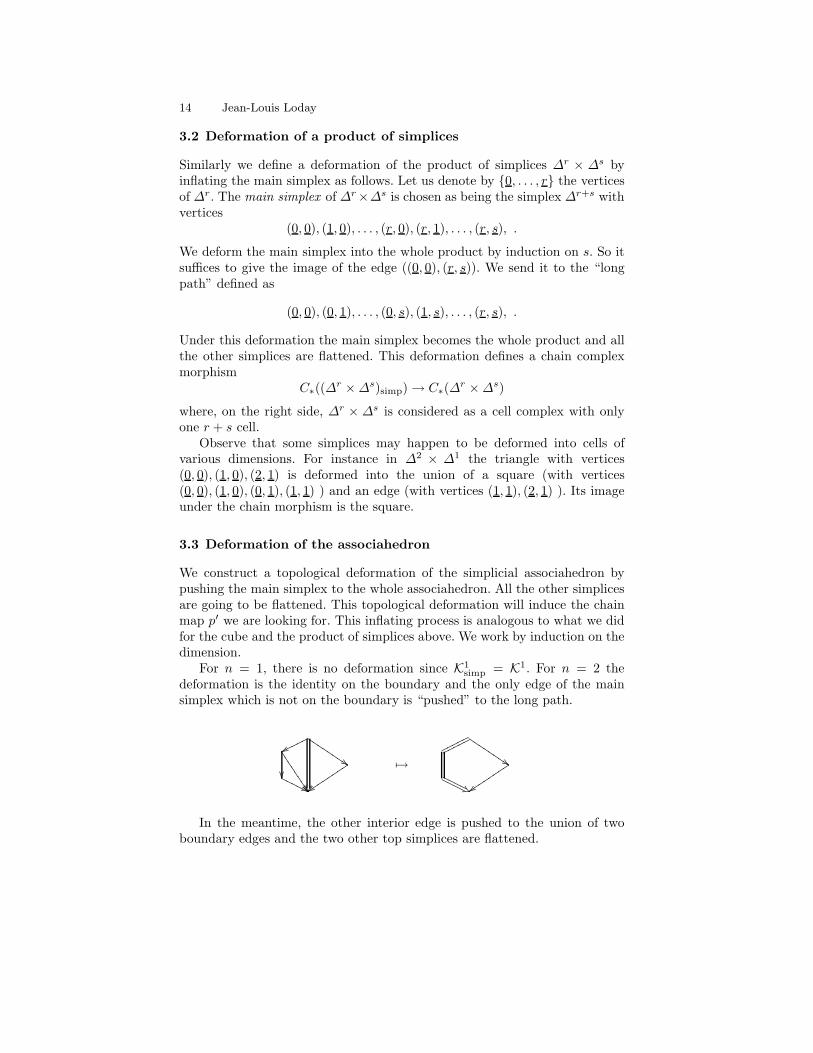
3.3 Deformation of the associahedron

We construct a topological deformation of the simplicial associahedron bypushing the main simplex to the whole associahedron. All the other simplicesare going to be flattened. This topological deformation will induce the chainmap p′ we are looking for. This inflating process is analogous to what we didfor the cube and the product of simplices above. We work by induction on thedimension.

For n = 1, there is no deformation since K1simp = K1. For n = 2 the

deformation is the identity on the boundary and the only edge of the mainsimplex which is not on the boundary is “pushed” to the long path.

wwooooo

$$JJJJJJ

JJ

444

4444

4

zztttttt

tt

''OOOOO7→

oooooooooo

$$JJJJJJ

JJ

zztttttt

tt

#+OOOOOOOO

In the meantime, the other interior edge is pushed to the union of twoboundary edges and the two other top simplices are flattened.


For higher n we use the inductive construction of Knsimp out of fatKn−1

simp.We suppose that the deformation is known for any i < n and we construct iton fatKn−1

simp. The simplicial set fatKn−1simp is the union of the simplicial sets of

the form Ktsimp = Ki

simp × Kjsimp indexed by some trees t with one and only

one internal edge. The main simplex of this product is the main simplex ∆i+j

of ∆i × ∆j where ∆i, resp. ∆j , is the main simplex of Kisimp, resp. Kj

simp.

The deformation is obtained by, first, deforming the main simplex ∆i+j into∆i×∆j as described in 3.2 and then use the inductive hypothesis (deformationfrom the main simplex to the associahedron).

The deformation of the interior cells is obtained by pushing the mainsimplex of Kn

simp to the top cell. It is determined by the image of the edges ofthe main simplex. By induction, it suffices to construct the image of the edgewhich goes from the vertex indexed by the left comb (initial element) to thevertex indexed by the right comb (terminal element). We choose to deform itto the long path of the associahedron as constructed in 1.2. Since any simplexof Kn

simp is either on the boundary, or is a cone (for the last vertex) over asimplex in the boundary, we are done. In particular, the edge going from a0-simplex labelled by the tree t to the right comb is deformed into a pathmade of 1-cells of the associahedron, constructed with the same rule as in theconstruction of the long path.

The deformed tetrahedron:

+3_g

GGGGGG

GGGGGG

GGGGGG

GGGGGG

ttttttttt

ttttttttt

ck OOOOOOOOOO

cc

GGGGGGGGGGGG

////

////

///

////

////

///

19

lllllllllllll

lllllllllllll _g

GGGGGGG

GGGGG

GGGGGGG

GGGGG

////

//

////

//

???

????

????

//

ttttttttt

ttttttttt

3.4 The map p′ : C∗(Kn

simp) → C∗(K

n)

We define the map p′ as follows. Under the deformation map any simplex ofKn

simp is sent to the union of cells of Kn. The image of such a simplex underp′ is the algebraic sum of the cells of the same dimension in the union. Forinstance, the main simplex is sent to the top cell (indexed by the corolla),and all the other top simplices are sent to 0, since under the deformation theyare flattened. From its topological nature it follows that p′ is a chain complexmorphism.

In low dimension we get the following. For n = 1, the map p′ is the identity.For n = 2, the map p′ is the identity on the 0-simplices and the 1-simplices ofthe boundary, and on the interior cells, we get:

16 Jean-Louis Loday

a =(

::::: , ::

::::: ,

:::::

:::::)

7→

:::::

((((

b =(

::::: ,

::

::::: ,

:::::

:::::)

7→ 0

c =(

::

::::: ,:::

::::: ,

:::::

:::::)

7→ 0

(

::::: ,

:::::

:::::)

7→

::::: +

::

::::: +

:::

:::::

(

::

::::: ,

:::::

:::::)

7→

::

::::: +

:::

:::::

Here are examples of the image under p′ of some interior 2-dimensionalsimplices for n = 3:

(

::::::: ,

:::::

::::::: ,

::::::::::

:::::::

)

7→

((((

::::::: +

::

:::::::

------

+

:::

:::::::

------ .

(

::

::::::: ,

:: ::

::::::: ,

::::::::::

:::::::

)

7→

::

:::::::

+

:::

::::::: +

:::::

((((

::::::: .

Proposition 3.5 The chain maps p′ : C∗(Knsimp) → C∗(K

n) assemble into a

morphism of dgns operads p′ : AA∞ → A∞.

Proof. We adopt the notation of 2.5 where the operadic composition mapγAA∞ is constructed. From this construction it follows that there is a mainsimplex in ω := γAA∞(ι0; ι1, . . . , ιn) if and only if all the simplices ιj are mainsimplices.

Supppose that one of them, say ιj is not a main simplex. Then we havep′(ιj) = 0, and therefore γA∞(p′(ι0); p

′(ι1), . . . , p′(ιn)) = 0. But since there is

no main simplex in ω, we also get p′(ω) = 0 as expected.


Suppose that all the simplices are main simplices. Then p′(ιj) = tijfor all

j and therefore γA∞(p′(ι0); p′(ι1), . . . , p

′(ιn)) = γA∞(ti0 ; ti1 , . . . , tin). On the

other hand ω contains the main simplex, therefore p′(ω) = γA∞(ti0 ; ti1 , . . . , tin)

and we are done.

Corollary 3.6 The composite

A∞q′

→ AA∞∆−→ AA∞ ⊗ AA∞

p′⊗p′

−→ A∞ ⊗ A∞ .

is a diagonal for the operad A∞.

Proof. It is immediate to check that this composite of dgns operad morphismssends µ2 to µ2 ⊗ µ2, since µ2 corresponds to the 0-cell of K0.

Proposition 3.7 If A is an associative algebra and B an A∞ algebra, then

the A∞-structure on A ⊗ B is given by

µn(a1 ⊗ b1, . . . , an ⊗ bn) = a1 · · · an ⊗ µn(b1, . . . , bn).

Proof. In the formula for ∆ we have µn = 0 for all n ≥ 3, that is, any treewith a k-valent vertex for k ≥ 3 is 0 on the left side. Hence the only termwhich is left is comb ⊗ corolla, whence the assertion.

3.8 The first formulas

Let us give the explicit form of ∆(µn) for n = 2, 3, 4:

∆( ??

) = ??

⊗ ??

,

∆(

????)

=

???? ⊗

???? +

???? ⊗??

???? ,

∆(

:::::

((((

)

=

::::: ⊗

:::::

(((( +

:::::

(((( ⊗

:::::

:::::

+

::::: ⊗

::

::::: −

::::: ⊗

:::

::::: −

::::: ⊗

::

::::: −

::

::::: ⊗

:::

::::: .

In this last formula the first three summands comes from the triangle(123, 141, 321), the next two summands come from the triangle (123, 213, 321)and the last summand comes from the last triangle (213, 312, 321). It is ex-actly the same formula as the one obtained by Saneblidze and Umble (cf. [13]example 1, [11] exercise 12). Topologically the diagonal of the pentagon isapproximated as a union of products of cells as follows:

18 Jean-Louis Loday

????

????

????

????

???

??

???

????

?

????

????

??

????

????

??

Each cell of this decomposition corresponds to a summand of the above for-mula, which indicates where the cell goes in the product K2 ×K2.

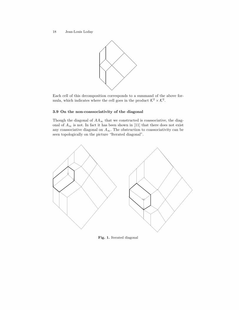
3.9 On the non-coassociativity of the diagonal

Though the diagonal of AA∞ that we constructed is coassociative, the diag-onal of A∞ is not. In fact it has been shown in [11] that there does not existany coassociative diagonal on A∞. The obstruction to coassociativity can beseen topologically on the picture “Iterated diagonal”.

Fig. 1. Iterated diagonal


Both pictures are the same combinatorially, except for an hexagon (high-lighted on the pictures), which is the union of 3 squares one way on the leftand the other way on the right. This is the obstruction to coassociativity. Ofcourse there is a way to reconcile these two decompositions via a homotopywhich is given by the cube.

Exercise 1. Show that the image of this cube in K2 × K2 ×K2 is indexed

by

::::: ×

::

::::: ×

:::

::::: .

Exercise 2. Compare the five iterated diagonals of the next step (some nicepictures to draw).

4 Comparing the operads AA∞ and ΩBAs

We first give a brief account of [11, 13] where a diagonal of the operad A∞

is constructed by using a coassociative diagonal on the dgns operad ΩBAs.Then we compare the two operads AA∞ and ΩBAs.

4.1 Cubical decomposition of the associahedron [1]

The associahedron can be decomposed into cubes as follows.For each tree t ∈ PBTn+2 we take a copy of the cube In (where I = [0, 1]

is the interval) which we denote by Int . Then the associahedron Kn is the

quotient

Kn :=⊔

t

Int / ∼

where the equivalence relation is as follows. We think of an element τ =(t; λ1, . . . , λn) ∈ In

t as a tree of type t where the λi’s are the lengths of theinternal edges. If some of the λi’s are 0, then the geometric tree determined byτ is not binary anymore (since some of its internal edges have been shrinkedto a point). We denote the new tree by τ . For instance, if none of the λi’s iszero, then τ = t ; if all the λi’s are zero, then the tree τ is the corolla (onlyone vertex). The equivalence relation τ ∼ τ ′ is defined by the following twoconditions:

- τ = τ ′,- the lengths of the nonzero-length edges of τ are the same as those of τ ′.Hence Kn is obtained as a cubical realization denoted Kn

cub.

Examples:

20 Jean-Louis Loday

????

////

//

????

???

////

//

????

????

K1 K2

4.2 Markl-Shnider version of Saneblidze-Umble diagonal [11, 13]

In [1] Boardman and Vogt showed that the bar-cobar construction on theoperad As is a dgns operad ΩBAs whose chain complex in arity n can beidentified with the chain complex of the cubical decomposition of the associ-ahedron:

(ΩBAs)n = C∗(Kn−2cub ) .

In [11] (where Kn−2cub is denoted Wn and Kn−2 is denoted Kn) Markl and

Shnider use this result to construct a coassociative diagonal on the operadΩBAs. There is a quasi-isomorphism q : A∞ → ΩBAs induced by the cubicaldecomposition of the associahedron (the image of the top cell is the the alge-braic sum of the cn−1 cubes). They construct an inverse quasi-isomorphismp : ΩBAs → A∞ by giving explicit algebraic formulas. At the chain level themap p : C∗(K

ncub) → C∗(K

n) has a topological interpretation using a defor-mation of the cubical associahedron as follows. The cube indexed by the leftcomb is called the main cube of the decomposition. The deformation sendsthe main cube to the top cell of the associahedron and flatten all the otherones.

Example:

#??

???

?

//

///

////

/

????

???

////

//

????

????

s oooooooo

'HHHHHHH

HHHHHHH

7→

w vvvvvvv

vvvvvvv

#+OOOOOOOO

The exact way the main cube is deformed is best explained by draw-ing the associahedron on the cube. This is recalled in the Appendix. In [4]Kadeishvili and Saneblidze give a general method for constructing a diagonalon some polytopes admitting a cubical decomposition along the same principle(inflating the main cube).

Markl and Shnider claim that the composite

A∞q→ ΩBAs → ΩBAs ⊗ ΩBAs

p⊗p−→ A∞ ⊗ A∞

is the Saneblidze-Umble diagonal.


5 Appendix 1: Drawing a Stasheff polytope on a cube

This is an account of some effort to construct the Stasheff polytope that I didin 2002 while visiting Northwestern University. During this visit I had the op-portunity to meet Samson Saneblidze and Ron Umble, who were drawing thesame kind of figures for different reasons (explained above). It makes the linkbetween Markl and Shnider algebraic description of the map p, the picturesappearing in Saneblidze and Umble paper, and some algebraic properties ofthe planar binary trees.

There is a way of constructing an associahedron structure on a cube asfollows. For n = 0 and n = 1 there is nothing to do since K0 and K1 arethe cubes I0 and I1 respectively. For n = 2, we simply add one point in themiddle of an edge to obtain a pentagon:

• // •

•

OO

•

OO

// •

OO

Inductively we draw Kn on In out of the drawing of Kn−1 on In−1 asfollows. Any tree t ∈ PBTn+1 gives rise to an ordered sequence of trees(t1, . . . , tk) in PBTn+2 as follows. We consider the edges which are on theright side of t, including the root. The tree t1 is formed by adding a leaf whichstarts from the middle of the root and goes rightward (see [6] p. 297). Thetree t2 is formed by adding a leaf which starts from the middle of the nextedge and goes rightward. And so forth. Obviously k is the number of verticeslying on the right side of t plus one (so it is always greater than or equal to2).

Example:

if t =??

???? , then t1 =

::

::::: , t2 =:::

::::: , t3 =

:::::

::::: .

In In = In−1 × I we label the point t × 0 by t1, the point t × 1by tk, and we introduce (in order) the points t2, . . . , tk−1 on the edge t× I.For n = 2 we obtain (with the coding introduced in section 1.1):

141 // 321

312

OO

123

OO

// 213

OO

22 Jean-Louis Loday

For n = 3 we obtain the following picture:

// ??

//

??

OO

??

//

OO

OO

??

OO

OO

//

OO

??

OO

//

??

OO

??

OO

(It is a good exercise to draw the tree at each vertex). Compare with [13],p. 3). The case n = 4 can be found on my home-page. It is important toobserve that the order induced on the vertices by the canonical orientationof the cube coincides precisely with the Tamari poset structure. The refereeinformed me that these pictures already appeared (without any mention ofthe Stasheff polytope) in [3].

Surprisingly, this way of viewing the associahedron is related to an alge-braic structure on the set of planar binary trees PBT =

⋃

n≥1 PBTn, relatedto dendriform algebras. Indeed there is a non-commutative monoid structureon the set of homogeneous nonempty subsets of PBT constructed in [6]. Itcomes from the associative structure of the free dendriform algebra on onegenerator. This monoid structure is denoted by +, the neutral element is thetree | . If t ∈ PBTp and s ∈ PBTq, then s + t is a subset of PBTp+q−1. It isproved in [6] that the trees which lie on the edge t × I ⊂ In are precisely

the trees of t + ??

. For instance:

???? + ??

=

::::: ∪ ::

:::::

and??

???? + ??

=

::

::::: ∪:::

::::: ∪

:::::

::::: .

The deformation of the associahedron consisting in inflating the main sim-plex to the top cell can be performed into two steps by considering a cubeinside the associahedron. This cube is determined by the previous construc-tion. First, we inflate the main simplex to the full cube as described in 3.1,then we deform the cube into the associahedron as indicated above.

Finally we remark that the deformation described in 3.3 permits us todraw the associahedron on the simplex.


6 Appendix 2: ∆(µ5)

In this appendix we give the computation of ∆(µ5) and we show that weget the same result as Saneblidze and Umble. In order to compare with theirresult we adopt their way of indexing the planar trees, which is as follows.Let t be a tree whose root vertex has k + 1 inputs, that we label (from left toright) by 0, . . . , k. Then, by definition, dij(t) is the tree obtained by replacing,locally, the root vertex by the following tree with one internal edge:

0 i i + j k

SSSSSSSSSSS · · ·JJJJ · · ·mmmmmm · · ·

hhhhhhhhhhhhhh

The operator dij is well-defined for 0 ≤ i ≤ k, 1 ≤ j ≤ k − i and (i, j) 6=(0, k). So we get:

ij = 01 02 11 12 21

dij

(

:::::

((((

)

=

:::::

:::::

::

:::::

:::

:::::

::

:::::

and d01d01

(

:::::

((((

)

=

::::: , etc.

Let us index the sixteen 3-simplices forming K3simp by the tree indexing

the face in fatK2simp and either a, b, c if this face is a pentagon (cf. 1.5) or the

shuffle α = (1, 2), β = (2, 1) if this face is a square (cf. 2.5). In the followingtableau we indicate the image of the 3-simplices under the map p′⊗p′∆AA∞ .In the left column we indicate the information which determines the 3-simplex(dij(µ5), x). In the right column we give its image (up to signs) as a sum offour terms, since in the AW morphism there are four terms.

24 Jean-Louis Loday

03 a (01)(01)(01)⊗ µ5 + (02)(01) ⊗(

− (21) + (22))

+(03) ⊗(

(11)(21) + (12)(21) + (11)(22))

+ µ5 ⊗ (11)(21)(31)03 b 0 + 0 + 0 + 003 c 0 + 0 + 0 + 002 α 0 + 0 + (02) ⊗

(

− (11)(31)− (12)(31))

+ 002 β 0 + (01)(02) ⊗

(

(11) + (12) + (13))

+ 0 + 001 a 0 + (01)(01) ⊗ (31) + (01) ⊗ (21)(31)01 b 0 + 0 + 0 + 001 c 0 + 0 + 0 + 012 α 0 + 0 + (12) ⊗

(

(12)(21) + (11)(22))

+ 012 β 0 + 0 + 0 + 011 a 0 + 0 − (11) ⊗ (12)(31) + 011 b 0 + (02)(11)⊗

(

(13) + (12))

+ 0 + 011 c 0 + (11)(11) ⊗ (13) + 0 + 021 a 0 + (11)(01) ⊗ (22) + (21) ⊗ (11)(22) + 021 b 0 + 0 + 0 + 021 c 0 + 0 + 0 + 0

As a result ∆(µ5) is the algebraic sum of 22 elements, which are exactlythe same as in [13] Example 1. Topologically, it means that K3 can be realizedas the union of 2 copies of K3 (having only one vertex in common), 6 copiesof K1 × K2, 6 copies of K2 × K1, 4 copies of (K1 ×K1) × K1 and 4 copies ofK1 × (K1 ×K1).

From this computation it is reasonable to conjecture that the diagonalconstructed from the simplicial decomposition of the associahedron is thesame as the Saneblidze-Umble diagonal.

References

1. J.M. Boardman, R.M. Vogt, Homotopy invariant algebraic structures on topo-logical spaces. Lecture Notes in Mathematics, Vol. 347. Springer-Verlag, Berlin-New York, 1973. x+257 pp.

2. M. Gaberdiel, B. Zwiebach, Tensor constructions of open string theories. I. Foun-dations. Nuclear Phys. B 505 (1997), no. 3, 569–624.

3. W. Geyer, On Tamari lattices. Discrete Math. 133 (1994), no. 1-3, 99–122.4. T. Kadeishvili, S. Saneblidze, The twisted Cartesian model for the double path

fibration, ArXiv math.AT/02102245. B. Keller, Introduction to A-infinity algebras and modules. Homology Homotopy

Appl. 3 (2001), no. 1, 1–35.6. J.-L. Loday, Arithmetree. J. Algebra 258 (2002), no. 1, 275–309.7. J.-L. Loday, Realization of the Stasheff polytope. Arch. Math. (Basel) 83 (2004),

no. 3, 267–278.8. J.-L. Loday, Parking functions and triangulation of the associahedron, Proceed-

ings of the Street’s fest, Contemporary Math. AMS 431, (2007), 327–340.9. S. MacLane, Homology. Die Grundlehren der mathematischen Wissenschaften,

Bd. 114 Academic Press, Inc., Publishers, New York; Springer-Verlag, Berlin-Gottingen-Heidelberg 1963 x+422 pp.


10. M. Markl, S. Shnider, J. Stasheff, Operads in algebra, topology and

physics. Mathematical Surveys and Monographs, 96. American MathematicalSociety, Providence, RI, 2002. x+349 pp.

11. M. Markl, S. Shnider, Associahedra, cellular W -construction and products ofA∞-algebras. Trans. Amer. Math. Soc. 358 (2006), no. 6, 2353–2372 (electronic).

12. A. Proute, A∞-structures, modele minimal de Baues-Lemaire et homologie desfibrations, These d’Etat, 1984, Universite Paris VII.

13. S. Saneblidze, R. Umble, A Diagonal on the Associahedra, preprint, ArXivmath.AT/0011065

14. S. Saneblidze, R. Umble, Diagonals on the permutahedra, multiplihedra andassociahedra. Homology Homotopy Appl. 6 (2004), no. 1, 363–411.

15. J.D. Stasheff, Homotopy associativity of H-spaces. I, II. Trans. Amer. Math.Soc. 108 (1963), 275-292; ibid. 293–312.

the diagonal of the stasheï¬€ polytope

Documents