The Diffusion of Cellular Telephony in Portugalbefore UMTS: A Time Series Approach

PEDRO PEREIRAAutoridade da Concorrência, R. Laura Alves, no 4, 4o, 1050-138 Lisboa (Portugal)

e-mail: jppereira@oninetspeed.pt; phone: 21-7802498; fax: 21-7802471

JOSÉ C. PERNÍAS-CERRILLOLEE and Economics Department, Universitat Jaume I, Castellón (Spain)

e-mail: jcpernias@ya.com; phone: 34-964728610

March 4, 2005

In this paper, we propose a methodology to estimate diffusion processes that differs from the standardpractice in two ways. First, we model the nonlinear long-run trend through the Richards curve, whichis more flexible than the standard alternatives. Second, we propose a dynamic specification thataccounts for: short-run dynamics, and a tendency to correct deviations from the nonlinear long-runtrend. We apply the model to the diffusion of cellular telephony in Portugal. Statistical tests showthat our model outperforms the standard diffusion models. We also use the model to characterize thediffusion process of the Portuguese cellular telephone industry, and test several hypothesis about therecent evolution of the industry.

1. INTRODUCTION

In the introduction we do two things. First, we give an overview of the paper’s methodology and results.Second, we review the literature.

1.1. Overview of the Paper

It is common practice in empirical studies on the diffusion of innovations over time, to assume that thenumber of individuals that adopt an innovation follows an S-shaped curve.1 After the introduction ofthe innovation, there is a initial stage where few individuals adopt the innovation. This early stage isfollowed by a period of rapid growth of the number of adopters. Finally, the diffusion process reachesa maturity phase, in which the growth of the number of adopters slows down, and the total number ofadopters gradually stabilizes.

The most used S-shaped growth curves in the empirical literature on diffusion are the logistic andGompertz curves.2 In spite of their “good fit”, these models display at least two serious shortcomings.The first and more important problem of these curves, is their lack of flexibility with respect to two im-portant characteristics of the diffusion process: (i) the inflection point, and (ii) the asymmetry aroundthe inflection point. For the logistic and Gompertz curves, the inflection point always occurs at a fixedfraction of the saturation level; 50% for the logistic and, approximately, 37% for Gompertz. The lo-gistic curve is symmetric around the time at which the inflection point occurs. The Gompertz curve isasymmetric, and the speed of adoption is larger in the later stages of the diffusion process. The second

1. Geroski (2000) discusses the theoretical arguments used to justify the S-shaped adoption curve.2. Both models have a long tradition in the literature of product and technology diffusion. Griliches (1957) is an early

example of the use of the logistic curve (see also Dixon, 1980). Chow (1967) uses the Gompertz curve.

problem of these curves is the difficulty of discriminating empirically between them. Typically, the com-parison of goodness of fit measures is inconclusive. Thus, in many cases, the model selection is doneon a subjective basis. This is specially problematic, since the predictions from the two models tend todiverge drastically, as the diffusion process evolves.

In this paper, we propose a methodology to estimate diffusion processes that differs from the standardpractice in two ways. First, we use the Richards curve, also known as generalized logistic curve, to modelthe diffusion trend. This slightly more complex, but still parsimonious model, does not impose rigidconstraints on the location of the inflection point, and allows the estimation of the degree of asymmetryaround the inflection point. Besides, it includes as a special case the logistic curve, and can approximatearbitrarily well the Gompertz curve. Thus, one can test explicitly those specifications against each other,without having resort to subjective considerations.3 The second way in which our approach differs fromthe standard practice, is that we propose a dynamic model, following the standard practice in moderntime series analysis, that accounts for both short-run and long-run related effects, and that uses exhaustivespecification testing for model selection (see Hendry, 1995).

The Portuguese cellular telephony industry provides a suitable application for the framework we havein mind. In Portugal, the firm associated with the incumbent, TMN, started its activity in 1989 with theanalogue technology C-450.4 In 1991, the sectoral regulator, ICP-ANACOM, assigned two licenses tooperate the digital technology GSM 900.5 One of the licenses was assigned to TMN. The other licensewas assigned to the entrant VODAFONE.6 In 1995, TMN pioneered internationally the introduction ofpre-paid cards. The proportion of subscribers that hold a pre-paid card increased quickly, and reachedwhat seems to be its steady state level of 79% in 1999. In 1997, the regulator assigned three licensesto operate the digital technology GSM 1800.7 Two licenses were assigned to TMN and VODAFONE. Athird license was assigned to the entrant OPTIMUS.8 In 1999, TMN discontinued the analogue service.The legislation of the E.U. imposed the full liberalization of the telecommunications industry at the endof the nineties.9 This meant that any firm licensed by the sectoral regulator could offer its services. Inparticular, any firm could offer fixed telephony services, either through direct access based on their owninfrastructures, or through indirect access, available for all types of calls. In Portugal the liberalizationtook effect in 2000.10 Finally, in 2001 ICP-ANACOM assigned licenses to operate the 3G technologyIMT2000/UMTS, and service began in 2004.

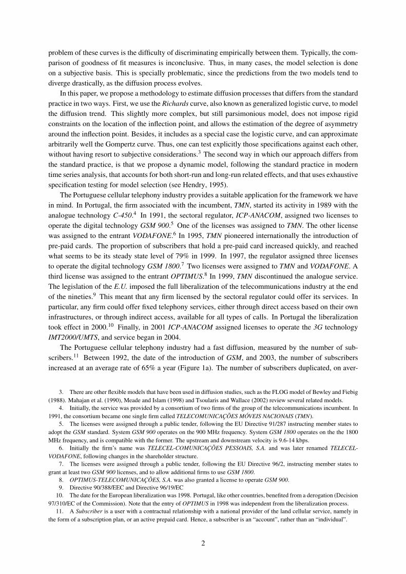
The Portuguese cellular telephony industry had a fast diffusion, measured by the number of sub-scribers.11 Between 1992, the date of the introduction of GSM, and 2003, the number of subscribersincreased at an average rate of 65% a year (Figure 1a). The number of subscribers duplicated, on aver-

3. There are other flexible models that have been used in diffusion studies, such as the FLOG model of Bewley and Fiebig(1988). Mahajan et al. (1990), Meade and Islam (1998) and Tsoularis and Wallace (2002) review several related models.

4. Initially, the service was provided by a consortium of two firms of the group of the telecommunications incumbent. In1991, the consortium became one single firm called TELECOMUNICAÇÕES MÓVEIS NACIONAIS (TMN).

5. The licenses were assigned through a public tender, following the EU Directive 91/287 instructing member states toadopt the GSM standard. System GSM 900 operates on the 900 MHz frequency. System GSM 1800 operates on the the 1800MHz frequency, and is compatible with the former. The upstream and downstream velocity is 9.6-14 kbps.

6. Initially the firm’s name was TELECEL-COMUNICAÇÕES PESSOAIS, S.A. and was later renamed TELECEL-VODAFONE, following changes in the shareholder structure.

7. The licenses were assigned through a public tender, following the EU Directive 96/2, instructing member states togrant at least two GSM 900 licenses, and to allow additional firms to use GSM 1800.

8. OPTIMUS-TELECOMUNICAÇÕES, S.A. was also granted a license to operate GSM 900.9. Directive 90/388/EEC and Directive 96/19/EC

10. The date for the European liberalization was 1998. Portugal, like other countries, benefited from a derogation (Decision97/310/EC of the Commission). Note that the entry of OPTIMUS in 1998 was independent from the liberalization process.

11. A Subscriber is a user with a contractual relationship with a national provider of the land cellular service, namely inthe form of a subscription plan, or an active prepaid card. Hence, a subscriber is an “account”, rather than an “individual”.

2

age, every 16.6 months. The speed of the diffusion lead to high and rising penetration rates.12 In 1999,the penetration rate of cellular telephony overtook the penetration rate of fixed telephony (Figure 1b). In2003 the penetration rate of fixed telephony was 40% and decreasing, and the rate of penetration of cel-lular telephony was 89% and increasing. The deployment of UMTS, conceivably, will give an additionalimpulse to cellular telephony.

Our objective is twofold. First, we want to evaluate the performance of our framework, comparedwith the standard approach. Second, we want to characterize the diffusion process of cellular telephony inPortugal before UMTS. We pay particular attention to three aspects. First, we are interested in whether theentry of OPTIMUS in 1998 increased the speed of the diffusion. The effects of competition on diffusionprocesses have received some attention on the literature.13 Conceivably, the entry of OPTIMUS in 1998,led the other two firms to lower their prices, and increase promotion. Either of these policies should haveincreased the speed of the diffusion. Second, we are interested in whether the full liberalization of thetelecommunications market in 2000 affected the speed of the diffusion of cellular telephony in Portugal.It is unclear what should have been the impact of the full liberalization of the telecommunications marketin Portugal. On the one hand, more competition in fixed telephony should have pushed the prices of thisservice down, and reduced the substitution between fixed and cellular telephony.14 On the other hand, theliberalization involved a tariff rebalancing which increased the telephone subscription fee and the priceof local calls. Third, we are interested whether there are network economies in the cellular telephoneindustry. The existence of network economies is one of the distinctive aspects of telecommunicationservices. Network interconnection obligations mitigate, but do not eliminate this effect. Differencesbetween intra and inter network calls resurface the value for a consumer of belonging to a large network.Empirical analysis confirms this perspective.15

Using quarterly data ranging from 1994 to 2003, we estimated several time series models, for the ag-gregate data, and for each of the three firms operating in Portugal. We used a battery of specification testsin order to asses the statistical properties of our regression models. The analysis shows that simpler mod-els that only add a disturbance term to a S-shaped trend present serious symptoms of misspecification.The dynamic effects we consider are important characteristics of the diffusion process. Including themin diffusion models enhances the statistical properties of the estimations. We think that our estimatesprovide a useful benchmark, with respect to which more structural models can be evaluated.

Our results indicate that the logistic curve is a valid statistical model for the diffusion process of cel-lular telephony in Portugal, but only as a long-term trend, from which data significantly and persistentlydeviates in the short-run. We found that the saturation level of the Portuguese cellular telephony marketfor GSM, implies a penetration rate around to 100%.16 Our results also provide an estimate of the periodat which the maturity phase began. Interestingly, the slowdown of the adoption of cellular telephonybegan in the year 2001, shortly after the full liberalization of the Portuguese telecommunications market.We found no evidence of a structural change in the diffusion process as a consequence of the liberaliza-tion process. However, the entrance of the third operator increased the speed of the diffusion process onthe short run, with little or no long-run effects. Finally, we investigated the cross-impacts of the diffusionprocesses of each firm in the market.

12. The Penetration Rate is the number of subscribers per 100 inhabitants.13. See Gruber and Verboven (2001a), Gruber and Verboven (2001b) and Gruber (2001) for recent contributions related

to the diffusion of cellular telephony. See Geroski (2000) and the papers cited therein for a more general discussion.14. Barros and Cadima (2000) document the substitution between cellular and fixed telephony in Portugal. See Rodini

et al. (2002) for the case of the US.15. See, e.g., Doganoglu and Grzybowski (2003).16. It has been argued that the industry is a natural oligopoly (Valletti, 2003). If true, this will depend on both the technol-

ogy, and the number of potential users. This gives a special importance to estimating the saturation level of the market.

3

0

1

2

3

4

5

6

7

8

9

10

1992 1993 1994 1995 1996 1997 1998 1999 2000 2001 2002 2003

TotalTMNVODAFONEOPTIMUS

(a) Total Number of Subscribers (in millions).

0

20

40

60

80

100

1992 1993 1994 1995 1996 1997 1998 1999 2000 2001 2002 2003

Fixed TelephonyCellular TelephonyEU Cellular Telephony Average

(b) Cellular Telephony Penetration Rates (%).

FIGURE 1Cellular Telephony Diffusion in Portugal

4

1.2. Literature Review

From a methodological point of view, our research draws from the literature on generalizations of thelogistic curve (Mahajan et al., 1990; Meade and Islam, 1998; Tsoularis and Wallace, 2002), and the mod-ern econometric approach to time series models (Hendry, 1995). Geroski (2000) surveys the literatureon new technology diffusion. Here we focus on the research directly related to our work.

Barros and Cadima (2000) estimated jointly the diffusion curves for cellular and fixed telephonyfor Portugal. They adopted the logistic curve for the diffusion of fixed telephony, and the Gompertzcurve for cellular telephony. In addition, they imposed a saturation level for cellular telephony thatimplied a penetration rate of 70%, and used as regressors variables like the prices of the services andgross domestic product per capita. They found a negative impact of the diffusion of cellular telephonyon the fixed telephony penetration rate. But no effect in the reverse direction. The data ranged from1993 to the third quarter of 1999. Botelho and Pinto (2000) fitted several curves to the Portuguese data.They concluded that the logistic provided the better fit, and estimated a saturation level that implies apenetration rate of 67.4%. The data ranged from 1989 to the second quarter of 2000.

Doganoglu and Grzybowski (2003) analyzed the cellular telephony industry in Germany from Janu-ary 1998 to June 2003. Their results suggest that network effects played a significant role in the diffusionof cellular services in Germany. Gruber and Verboven (2001a) analyzed the technological and regulatorydeterminants of the diffusion of cellular telephony in the E.U., using a logistic model of diffusion. Theyfound that the transition from the analogue to the digital technology during the early nineties, and thecorresponding increase in spectrum capacity, had a major impact on the diffusion of cellular telephony.The impact of introducing competition has also been significant, during both the analogue and the digitalperiod, though the effect was small compared to the technology effect. Gruber (2001) analyzed the dif-fusion of cellular telephony in Central and Eastern Europe. They found that about 20% of the populationwill adopt cellular telephony, and that the speed of diffusion increased with the number of firms.

The remainder of the paper is organized as follows. Section 2 describes the Richards’ curve. Sec-tion 2 discusses a dynamic diffusion model that it is used to estimate the main characteristics of thediffusion process. In Section 3, we apply an extended dynamic model to each of the firms operating inthe Portuguese market. Section 5 concludes.

2. THE RICHARDS CURVE

2.1. The Model

The Richards curve is an S-shaped deterministic function of time.17 If N(t) follows a Richards curve,then:

N(t) = κ[1+ µe−γ(1+µ)(t−τ)]−1/µ

, (1)

The parametrization of the Richards curve given in equation (1) simplifies the interpretation of the para-meters. Parameter κ > 0 is the saturation level, i.e., limt→∞ N(t) = κ; parameter τ is the time period atwhich N(t) has an inflection point , i.e., the period at which maximal absolute growth occurs; parameterγ > 0 is the relative growth rate at time t = τ; and µ ≥ 0 is a shape parameter related to the degree ofasymmetry of the adoption process.

Equation (1) encompasses several special cases. We will only discuss the two cases commonly usedin the economics literature on the diffusion of innovations: (i) the logistic curve, and (ii) the Gompertzcurve.

17. Richards (1959) first introduced a generalization of the logistic curve (see also Nelder, 1962), and Nelder (1961) usedit for estimation purposes.

5

If µ = 1 thenN(t) = κ

[1+ e−2γ(t−τ)]−1

, (2)

which is the Logistic curve.As µ tends to 0 the Richards curve (1) tends to the Gompertz curve. Rewrite (1) as:

(N(t)/κ)µ −1µ

=−(eγ(1+µ)(t−τ) + µ)−1. (3)

The left side of equation (3) is the Box-Cox transformation of N(t)/κ . Thus, when µ tends to 0, bothsides of equation (3) tend to:

ln(N(t)/κ) =−e−γ(t−τ). (4)

Solving for N(t) yieldsN(t) = κe−e−γ(t−τ)

, (5)

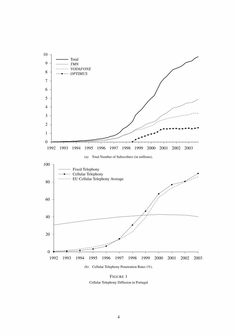
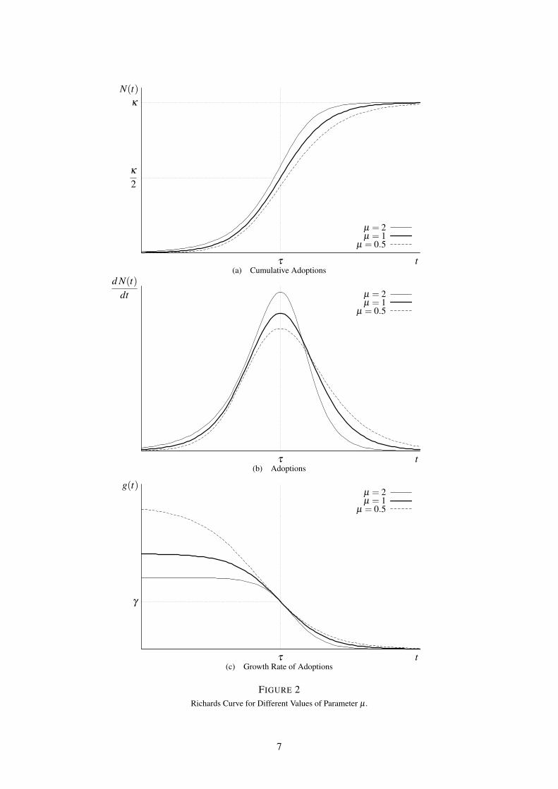
which is the Gompertz curve.Figure 2a plots the Richards curve for three values of parameter µ . The logistic curve, µ = 1, imposes

the constraint that the inflection point occurs when half of the diffusion took place, i.e., N(τ) = κ/2 ifµ = 1. Values of µ larger than 1 imply that the inflection point occurs at higher levels of adoption,i.e., N(τ) > κ/2 if µ > 1. And, limµ→∞ N(τ) = κ . Conversely, N(τ) < κ/2 if µ < 1. In this case,limµ→0 N(τ) = e−1κ , which correspond to the inflection point of the Gompertz curve. In the generalcase, the inflection point is N(τ) = κ/(1+ µ)1/µ .

Figure 2b plots the number of new subscribers per period, d N(t)/d t, for various values of parameterµ . The maximum number of adoptions occurs at period t = τ , at which the inflection point occurs. Animportant feature of logistic curve is that the number of adoptions is symmetric around τ . Values ofµ larger than 1 imply a fatter left tail than the logistic curve, and values of µ smaller 1 imply a fatterright tail. Hence, as µ increases, the slowdown in the adoption process after period t = τ is increasinglypronounced.

Taking logarithms and differentiating (1), one obtain the growth rate of N(t) as:

g(t) =d lnN(t)

dt=

γ(1+ µ)eγ(1+µ)(t−τ) + µ

=γ(1+ µ)

µ

[1−

(N(t)

κ

)µ](6)

Figure 2c plots the growth rate of N(t) for different values of parameter µ . The last equality of Equa-tion (6) is very informative. Ratio γ(1+ µ)/µ is called the “natural rate of growth”. It can be interpretedas the rate of growth that would occur, if there were no constraints limiting the adoption process, i.e.,no saturation level, and the diffusion process could grow without limits. The term in square brackets,[1− (N(t)/κ)µ

], shows the decay of the growth rate over time, as the number of adopters increases. In

the case of the logistic curve, µ = 1, the decay is linear in the cumulative number of subscribers. In othercases where µ 6= 1, the decay is a nonlinear function of N(t). As an example, in the limiting case of theGompertz curve, i.e., as µ tends to 0, g(t) =−γ ln(N(t)/κ).

2.2. An Illustration

Next we use the Richards curve to characterize the adoption of cellular telephones in Portugal. We usethe following empirical specification:

yt = N(t)eut , (7)

where yt is the number of subscribers in millions, N(t) is the deterministic trend given in (1), and ut

is a regression disturbance, which is supposed to have the usual properties of no serial dependence,

6

tτ

N(t)

κ

2

κ

µ = 2µ = 1

µ = 0.5

(a) Cumulative Adoptions

tτ

d N(t)dt µ = 2

µ = 1µ = 0.5

(b) Adoptions

tτ

g(t)

γ

µ = 2µ = 1

µ = 0.5

(c) Growth Rate of Adoptions

FIGURE 2Richards Curve for Different Values of Parameter µ .

7

homoskedasticity, and normal distribution.18 Taking logarithms in equation (7), we obtain:

lnyt = lnN(t)+ut = lnκ− 1µ

ln[1+ µe−γ(1+µ)(t−τ)]+ut . (8)

We estimate the parameters of the above nonlinear regression model through the maximum-likelihoodmethod.19 The selection of starting values for the parameters of equation (8) was the only practicaldifficulty encountered when estimating. The preceding discussion on the interpretation of parametershelped us in this task. For parameter κ we used the maximum of yt . For parameter µ we used a startingvalue of 1, the logistic curve case. For parameter τ we plotted the first difference of yt , and guessedvisually at which time period it attained the maximum.20 And finally, for parameter γ , we examined thegrowth rate of yt around the guessed value for τ . With these starting values, convergence was achievedin a few iterations.

The results of the estimation are presented in Table 1.21 We report three sets of estimates for: (i) theRichards curve, (ii) the logistic curve, obtained by restricting µ to equal 1, and (iii) the Gompertz curve,obtained by restricting µ to equal 0.

From Table 1, the parameter estimates vary considerably across the three models. For example,the estimated saturation level is around 9.3 millions subscribers for the Richards curve, but around 47millions for the Gompertz curve. Observe that, in spite of the large differences in the estimates of thelogistic and Gompertz specifications, they provide a similar fit to the data, as measured by the R̄2. Weused the Wald tests, reported in the last row of Table 1, to discriminate between these three models. Boththe logistic and the Gompertz curves were strongly rejected in favor of the more general Richards model.

A standard 95% confidence interval estimator of the saturation level for the Richards curve rangesfrom 8.7 to 10.0 millions. The estimate of τ is not significantly different from 0. According to thenormalization we adopted for t, this is compatible with the inflection point of N(t) being located at thefirst quarter of year 2000. From the estimated value of µ , the implied inflection point took place whenthe cumulative adoptions reached the 56% of the saturation level.

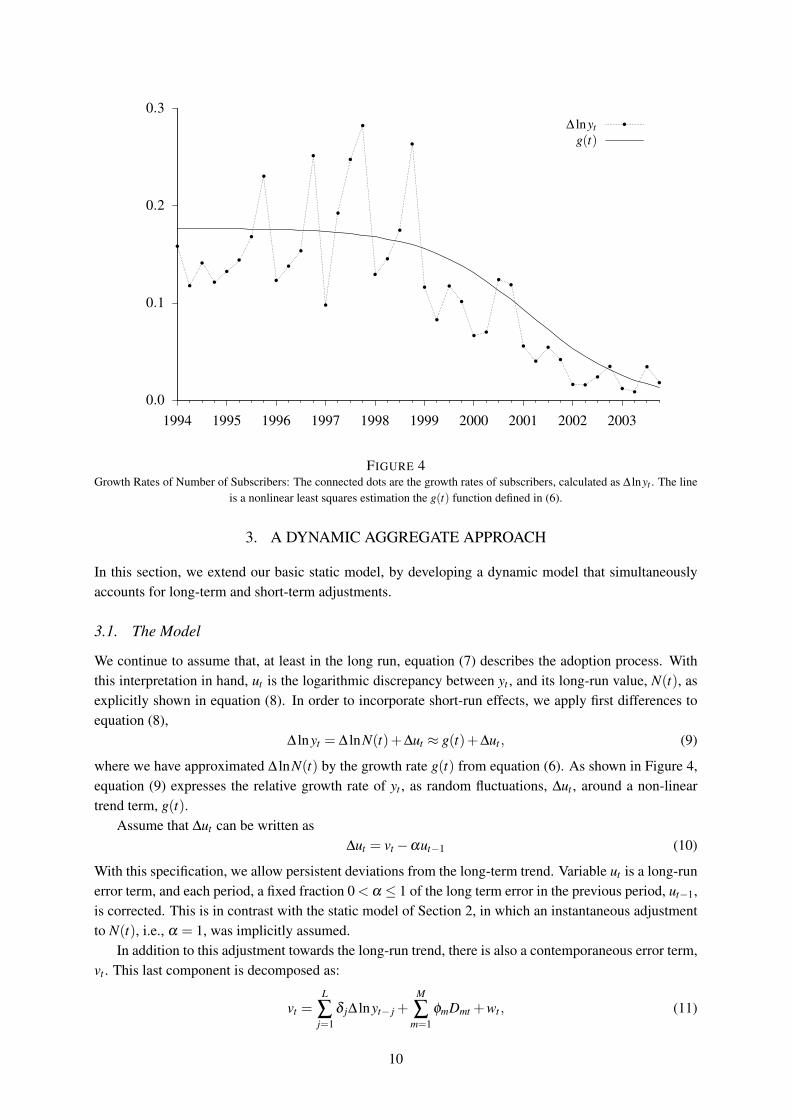
The goodness of fit, measured by the R̄2, is very close to 1. However, this is not surprising given thestrong trend showed by the data. There are also clear symptoms that equation (7) is misspecified. The lowvalue of the Durbin-Watson statistic indicates the presence of a strong pattern of positive autocorrelationin the residuals confirmed by visual inspection of Figure 3. A complete set of statistical tests, not reportedhere, points to the existence of: (i) a strong pattern of serial dependence of ut , both in the form of residualautocorrelation, and in the form of autoregressive conditional heteroskedasticity; (ii) heteroskedasticityof the error term; and (iii) functional form misspecification. These observations cast doubts on thevalidity of the estimations presented in Table 1, and, in particular, on the validity of the Wald tests ofTable 1, used to discriminate among the three models.

18. From (7), we use a multiplicative error term. Three reasons favor our specification over the commonly used additiveerror term. First, the estimation residuals are better behaved. Second, the multiplicative specification fits better with the dynamicmodel discussed in the following section. And third, the multiplicative model is logically coherent, in the sense that it allows aunbounded normally distributed disturbance term, while at the same time, the dependent variable is bounded.

19. All econometric results were obtained with Eviews 3.1.20. Parameter τ is measured in the same units used for t. Thus, for ease of interpretation of parameter τ , t was normalized

to be 0 on the first quarter of 2000, 1 on the second quarter of 2000, and so on.21. Our data consists in the number of subscribers per firm, and was obtained from the firms. For TMN we have annual

observations from 1989 to 1991, and quarterly observations from 1992 to the end of 2003. For VODAFONE, we have anannual observation for 1992, and quarterly observations from 1993 to the end of 2003. And for OPTIMUS, we have quarterlyobservations from the third quarter of 1998 to the end of 2003. From this data we have constructed the total number ofsubscribers covering the period from the first quarter of 1993 to the last quarter of 2003. The sample used in the regressionsof Table 1 covers the period 1994.I to 2003.IV to ease the comparison with the dynamic specifications presented in sections 3and 4.

8

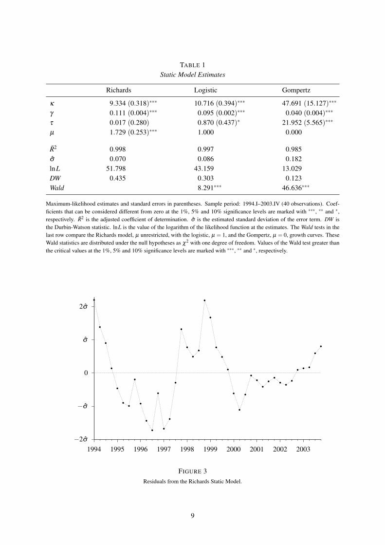
TABLE 1Static Model Estimates

Richards Logistic Gompertz

κ 9.334 (0.318)∗∗∗ 10.716 (0.394)∗∗∗ 47.691 (15.127)∗∗∗

γ 0.111 (0.004)∗∗∗ 0.095 (0.002)∗∗∗ 0.040 (0.004)∗∗∗

τ 0.017 (0.280) 0.870 (0.437)∗ 21.952 (5.565)∗∗∗

µ 1.729 (0.253)∗∗∗ 1.000 0.000

R̄2 0.998 0.997 0.985σ̂ 0.070 0.086 0.182lnL 51.798 43.159 13.029DW 0.435 0.303 0.123Wald 8.291∗∗∗ 46.636∗∗∗

Maximum-likelihood estimates and standard errors in parentheses. Sample period: 1994.I–2003.IV (40 observations). Coef-ficients that can be considered different from zero at the 1%, 5% and 10% significance levels are marked with ∗∗∗, ∗∗ and ∗,respectively. R̄2 is the adjusted coefficient of determination. σ̂ is the estimated standard deviation of the error term. DW isthe Durbin-Watson statistic. lnL is the value of the logarithm of the likelihood function at the estimates. The Wald tests in thelast row compare the Richards model, µ unrestricted, with the logistic, µ = 1, and the Gompertz, µ = 0, growth curves. TheseWald statistics are distributed under the null hypotheses as χ2 with one degree of freedom. Values of the Wald test greater thanthe critical values at the 1%, 5% and 10% significance levels are marked with ∗∗∗, ∗∗ and ∗, respectively.

2σ̂

σ̂

0

−σ̂

−2σ̂

1994 1995 1996 1997 1998 1999 2000 2001 2002 2003

FIGURE 3Residuals from the Richards Static Model.

9

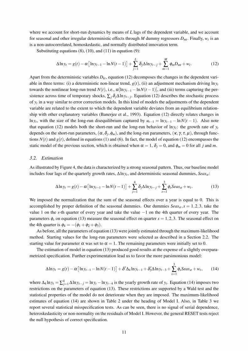
0.0

0.1

0.2

0.3

1994 1995 1996 1997 1998 1999 2000 2001 2002 2003

∆ lnytg(t)

FIGURE 4Growth Rates of Number of Subscribers: The connected dots are the growth rates of subscribers, calculated as ∆ lnyt . The line

is a nonlinear least squares estimation the g(t) function defined in (6).

3. A DYNAMIC AGGREGATE APPROACH

In this section, we extend our basic static model, by developing a dynamic model that simultaneouslyaccounts for long-term and short-term adjustments.

3.1. The Model

We continue to assume that, at least in the long run, equation (7) describes the adoption process. Withthis interpretation in hand, ut is the logarithmic discrepancy between yt , and its long-run value, N(t), asexplicitly shown in equation (8). In order to incorporate short-run effects, we apply first differences toequation (8),

∆ lnyt = ∆ lnN(t)+∆ut ≈ g(t)+∆ut , (9)

where we have approximated ∆ lnN(t) by the growth rate g(t) from equation (6). As shown in Figure 4,equation (9) expresses the relative growth rate of yt , as random fluctuations, ∆ut , around a non-lineartrend term, g(t).

Assume that ∆ut can be written as∆ut = vt −αut−1 (10)

With this specification, we allow persistent deviations from the long-term trend. Variable ut is a long-runerror term, and each period, a fixed fraction 0 < α ≤ 1 of the long term error in the previous period, ut−1,is corrected. This is in contrast with the static model of Section 2, in which an instantaneous adjustmentto N(t), i.e., α = 1, was implicitly assumed.

In addition to this adjustment towards the long-run trend, there is also a contemporaneous error term,vt . This last component is decomposed as:

vt =L

∑j=1

δ j∆ lnyt− j +M

∑m=1

φmDmt +wt , (11)

10

where we account for short-run dynamics by means of L lags of the dependent variable, and we accountfor seasonal and other irregular deterministic effects through M dummy regressors Dmt . Finally, wt is anis a non-autocorrelated, homoskedastic, and normally distributed innovation term.

Substituting equations (8), (10), and (11) in equation (9):

∆ lnyt = g(t)−α[

lnyt−1− lnN(t−1)]+

L

∑j=1

δ j∆ lnyt− j +M

∑m=1

φmDmt +wt . (12)

Apart from the deterministic variables Dkt , equation (12) decomposes the changes in the dependent vari-able in three terms: (i) a deterministic non-linear trend, g(t), (ii) an adjustment mechanism driving lnyt

towards the nonlinear long-run trend N(t), i.e., α[lnyt−1− lnN(t−1)], and (iii) terms capturing the per-sistence across time of temporary shocks, ∑ j δ j∆ lnyt− j. Equation (12) describes the stochastic processof yt in a way similar to error correction models. In this kind of models the adjustments of the dependentvariable are related to the extent to which the dependent variable deviates from an equilibrium relation-ship with other explanatory variables (Banerjee et al., 1993). Equation (12) directly relates changes inlnyt , with the size of the long-run disequilibrium captured by ut−1 = lnyt−1− lnN(t − 1). Also notethat equation (12) models both the short-run and the long-run behavior of lnyt : the growth rate of yt

depends on the short-run parameters, (α,δ j,φm), and the long-run parameters, (κ,γ,τ,µ), through func-tions N(t) and g(t), defined in equations (1) and (6). In fact, the model of equation (12) encompasses thestatic model of the previous section, which is obtained when α = 1, δ j = 0, and φm = 0 for all j and m.

3.2. Estimation

As illustrated by Figure 4, the data is characterized by a strong seasonal pattern. Thus, our baseline modelincludes four lags of the quarterly growth rates, ∆ lnyt , and deterministic seasonal dummies, Seasst :

∆ lnyt = g(t)−α[

lnyt−1− lnN(t−1)]+

4

∑j=1

δ j∆ lnyt− j +3

∑s=1

φsSeasst +wt . (13)

We imposed the normalization that the sum of the seasonal effects over a year is equal to 0. This isaccomplished by proper definition of the seasonal dummies. Our dummies Seasst ,s = 1,2,3, take thevalue 1 on the s-th quarter of every year and take the value −1 on the 4th quarter of every year. Theparameters φs on equation (13) measure the seasonal effect on quarter s = 1,2,3. The seasonal effect onthe 4th quarter is φ4 =−(φ1 +φ2 +φ3).

As before, all the parameters of equation (13) were jointly estimated through the maximum-likelihoodmethod. Starting values for the long-run parameters were selected as described in a Section 2.2. Thestarting value for parameter α was set to α = 1. The remaining parameters were initially set to 0.

The estimation of model in equation (13) produced good results at the expense of a slightly overpara-metrized specification. Further experimentation lead us to favor the more parsimonious model:

∆ lnyt = g(t)−α[

lnyt−1− lnN(t−1)]+δ

′∆4 lnyt−1 +δ

′3∆ lnyt−3 +

3

∑s=1

φsSeasst +wt , (14)

where ∆4 lnyt = ∑4j=1 ∆ lnyt− j = lnyt− lnyt−4 is the yearly growth rate of yt . Equation (14) imposes two

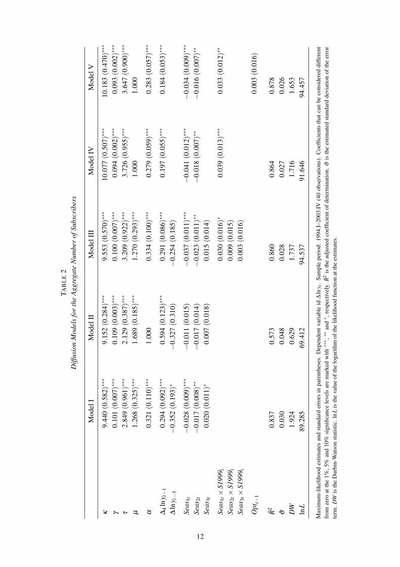
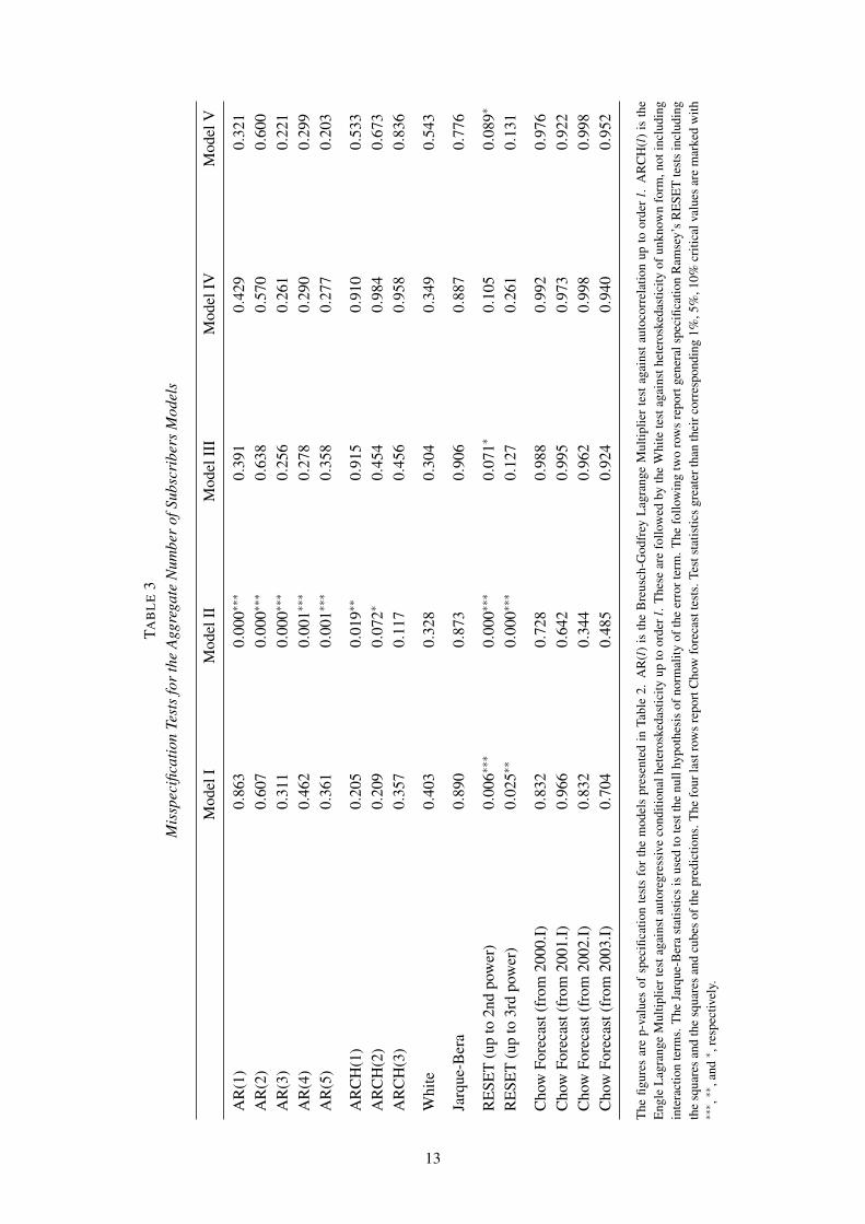
restrictions on the parameters of equation (13). These restrictions are supported by a Wald test and thestatistical properties of the model do not deteriorate when they are imposed. The maximum-likelihoodestimates of equation (14) are shown in Table 2 under the heading of Model I. Also, in Table 3 wereport several statistical misspecification tests. As can be seen, there is no signal of serial dependence,heteroskedasticity or non-normality on the residuals of Model I. However, the general RESET tests rejectthe null hypothesis of correct specification.

11

TAB

LE

2D

iffus

ion

Mod

els

for

the

Agg

rega

teN

umbe

rof

Subs

crib

ers

Mod

elI

Mod

elII

Mod

elII

IM

odel

IVM

odel

V

κ9.

440

(0.5

82)∗∗∗

9.15

2(0

.284

)∗∗∗

9.55

3(0

.570

)∗∗∗

10.0

77(0

.507

)∗∗∗

10.1

83(0

.470

)∗∗∗

γ0.

101

(0.0

07)∗∗∗

0.10

9(0

.003

)∗∗∗

0.10

0(0

.007

)∗∗∗

0.09

4(0

.002

)∗∗∗

0.09

3(0

.002

)∗∗∗

τ2.

849

(0.9

61)∗∗∗

2.12

9(0

.387

)∗∗∗

3.20

9(0

.922

)∗∗∗

3.72

6(0

.955

)∗∗∗

3.64

7(0

.900

)∗∗∗

µ1.

268

(0.3

25)∗∗∗

1.68

9(0

.185

)∗∗∗

1.27

0(0

.293

)∗∗∗

1.00

01.

000

α0.

321

(0.1

10)∗∗∗

1.00

00.

334

(0.1

00)∗∗∗

0.27

9(0

.059

)∗∗∗

0.28

3(0

.057

)∗∗∗

∆4

lny t−

10.

294

(0.0

92)∗∗∗

0.59

4(0

.123

)∗∗∗

0.29

1(0

.086

)∗∗∗

0.19

7(0

.055

)∗∗∗

0.18

4(0

.053

)∗∗∗

∆ln

y t−

3−

0.35

2(0

.193

)∗−

0.32

7(0

.310

)−

0.25

4(0

.185

)

Seas

1t−

0.02

8(0

.009

)∗∗∗

−0.

011

(0.0

15)

−0.

037

(0.0

11)∗∗∗

−0.

041

(0.0

12)∗∗∗

−0.

034

(0.0

09)∗∗∗

Seas

2t−

0.01

7(0

.008

)∗∗

−0.

017

(0.0

14)

−0.

023

(0.0

11)∗∗

−0.

018

(0.0

07)∗∗

−0.

016

(0.0

07)∗∗

Seas

3t0.

020

(0.0

11)∗

0.00

7(0

.018

)0.

015

(0.0

14)

Seas

1t×

S199

9 t0.

030

(0.0

16)∗

0.03

9(0

.013

)∗∗∗

0.03

3(0

.012

)∗∗

Seas

2t×

S199

9 t0.

009

(0.0

15)

Seas

3t×

S199

9 t0.

003

(0.0

16)

Opt

t−1

0.00

3(0

.016

)

R̄2

0.83

70.

573

0.86

00.

864

0.87

8σ̂

0.03

00.

048

0.02

80.

027

0.02

6D

W1.

924

0.62

91.

737

1.71

61.

653

lnL

89.2

8569

.412

94.5

3791

.646

94.4

57

Max

imum

-lik

elih

ood

estim

ates

and

stan

dard

erro

rsin

pare

nthe

ses.

Dep

ende

ntva

riab

leid

∆ln

y t.

Sam

ple

peri

od:

1994

.I–20

03.IV

(40

obse

rvat

ions

).C

oeffi

cien

tsth

atca

nbe

cons

ider

eddi

ffer

ent

from

zero

atth

e1%

,5%

and

10%

sign

ifica

nce

leve

lsar

em

arke

dw

ith∗∗∗ ,∗∗

and∗ ,

resp

ectiv

ely.

R̄2

isth

ead

just

edco

effic

ient

ofde

term

inat

ion.

σ̂is

the

estim

ated

stan

dard

devi

atio

nof

the

erro

rte

rm.D

Wis

the

Dur

bin-

Wat

son

stat

istic

.ln

Lis

the

valu

eof

the

loga

rith

mof

the

likel

ihoo

dfu

nctio

nat

the

estim

ates

.

12

TAB

LE

3M

issp

ecifi

catio

nTe

sts

for

the

Agg

rega

teN

umbe

rof

Subs

crib

ers

Mod

els

Mod

elI

Mod

elII

Mod

elII

IM

odel

IVM

odel

V

AR

(1)

0.86

30.

000∗∗∗

0.39

10.

429

0.32

1A

R(2

)0.

607

0.00

0∗∗∗

0.63

80.

570

0.60

0A

R(3

)0.

311

0.00

0∗∗∗

0.25

60.

261

0.22

1A

R(4

)0.

462

0.00

1∗∗∗

0.27

80.

290

0.29

9A

R(5

)0.

361

0.00

1∗∗∗

0.35

80.

277

0.20

3

AR

CH

(1)

0.20

50.

019∗∗

0.91

50.

910

0.53

3A

RC

H(2

)0.

209

0.07

2∗0.

454

0.98

40.

673

AR

CH

(3)

0.35

70.

117

0.45

60.

958

0.83

6

Whi

te0.

403

0.32

80.

304

0.34

90.

543

Jarq

ue-B

era

0.89

00.

873

0.90

60.

887

0.77

6

RE

SET

(up

to2n

dpo

wer

)0.

006∗∗∗

0.00

0∗∗∗

0.07

1∗0.

105

0.08

9∗

RE

SET

(up

to3r

dpo

wer

)0.

025∗∗

0.00

0∗∗∗

0.12

70.

261

0.13

1

Cho

wFo

reca

st(f

rom

2000

.I)0.

832

0.72

80.

988

0.99

20.

976

Cho

wFo

reca

st(f

rom

2001

.I)0.

966

0.64

20.

995

0.97

30.

922

Cho

wFo

reca

st(f

rom

2002

.I)0.

832

0.34

40.

962

0.99

80.

998

Cho

wFo

reca

st(f

rom

2003

.I)0.

704

0.48

50.

924

0.94

00.

952

The

figur

esar

ep-

valu

esof

spec

ifica

tion

test

sfo

rth

em

odel

spr

esen

ted

inTa

ble

2.A

R(l

)is

the

Bre

usch

-God

frey

Lag

rang

eM

ultip

lier

test

agai

nsta

utoc

orre

latio

nup

toor

der

l.A

RC

H(l

)is

the

Eng

leL

agra

nge

Mul

tiplie

rtes

taga

inst

auto

regr

essi

veco

nditi

onal

hete

rosk

edas

ticity

upto

orde

rl.

The

sear

efo

llow

edby

the

Whi

tete

stag

ains

thet

eros

keda

stic

ityof

unkn

own

form

,not

incl

udin

gin

tera

ctio

nte

rms.

The

Jarq

ue-B

era

stat

istic

sis

used

tote

stth

enu

llhy

poth

esis

ofno

rmal

ityof

the

erro

rter

m.T

hefo

llow

ing

two

row

sre

port

gene

rals

peci

ficat

ion

Ram

sey’

sR

ESE

Tte

sts

incl

udin

gth

esq

uare

san

dth

esq

uare

san

dcu

bes

ofth

epr

edic

tions

.The

four

last

row

sre

port

Cho

wfo

reca

stte

sts.

Test

stat

istic

sgr

eate

rtha

nth

eirc

orre

spon

ding

1%,5

%,1

0%cr

itica

lval

ues

are

mar

ked

with

∗∗∗ ,∗∗

,and

∗ ,re

spec

tivel

y.

13

The estimates of Model I of the long run parameters κ and γ are similar to those obtained with thesimpler static model of Table 1. But the estimates of the time at which inflection occurs, τ , and the shapeparameter, µ are very different. The estimate of τ for Model I implies that the inflection occurred at theend of year 2000. Also, the estimate of parameter µ is not significantly different from 1, so we fail toreject the hypothesis of a symmetric long-run trend.

The poor performance of the static model of the previous section could be caused by the omission ofshort run dynamics and seasonal effects. Model II is designed to provide a fairer comparison, allowingfor seasonal effects and short-run dynamics but imposing an instantaneous adjustment to the non-lineartrend, α = 1. Model II is clearly worse than Model I. The huge reduction in the fit rejects the hypothesisα = 1, and the misspecification tests show a substantial amount of serial dependence in the residuals.Therefore, we conclude that slow adjustment to the nonlinear trend is an important feature of our data.Failing to account this, seriously bias the estimates of the parameters driving the diffusion process.

As said before, Model I fails to pass the RESET tests. This could be due to the varying pattern ofseasonality in our data, clearly illustrated in Figure 4, but not accounted in Model I. We have extendedModel I by adding the interactions of the seasonal dummies, Seasst , with a step dummy, S1999t , whichtakes value 0 for observations preceding year 1999 and 1 for year 1999 and on. The coefficients ofthese interaction variables measure the change in the seasonal pattern from 1999. The estimates of theextended model are reported under the heading Model III in Table 2. The estimates of Model III suggestsa change in seasonality affecting especially to the effect of the first quarter. The statistical properties ofModel III are better than those of Model I: only one RESET test rejects the null hypothesis at the 10%significance level.

Model IV imposes some restrictions on the parameters of Model III. First, we impose the hypothesisof a logistic long-run trend, µ = 1. Second, we set to 0 the insignificant parameters of Model III. Theserestrictions are not rejected by a Wald test, and, in fact, the goodness of fit, measured by the R̄2, isslightly better. The misspecification tests of Table 3 do not signal any problem with Model IV. Alsothe Chow forecast tests do not signal problems of parameter instability. With respect to the short-rundynamics, it is worth noting that the estimate of the parameter associated with the lagged yearly growthrate, ∆4 lnyt−1, is positive and significantly different from 0. This could be interpreted as evidence infavor of the existence of network economies. An increase in the growth rate of the number of subscribersaccelerates the adoption process in subsequent periods.

Model V of Table 2 is estimated to analyze the impact of the entrance of OPTIMUS in the market.This model extends Model IV by adding a dummy variable Optt which takes value 1 on 1998.III, coin-ciding with the OPTIMUS entrance, and 0 otherwise. Observe that this dummy enters in Model V laggedone period, so the effect of the entrance occurs one quarter after the entrance. We experimented withother specifications, but we detected no structural change in the parameters around the time the entranceoccurred.

3.3. Analysis

Further inspection of Table 2 leads to the following observations.

Observation 3.1. A logistic long-run trend is a valid model for the Portuguese cellular telephoneindustry. �

From Table 2, one fails to reject the hypothesis that µ = 1. This conclusion might come as a surpriseafter the build up of Section 2. But in fact what it does is highlight, once again, the inadequacy of thestatic approach.

14

Observation 3.2. The saturation level for GSM ranges between 9.2 and 11.1 millions subscribers.�

This conclusion is supported by a 95% confidence interval estimate for the κ parameter constructedfrom Model V of Table 2. The diffusion of GSM had almost concluded by the end of 2003. Very likely,the deployment of UMTS will give an additional impulse to the diffusion process.

Observation 3.3. The inflection point occurred in the fourth quarter of 2000. �

This conclusion follows from the estimated value of τ parameter. This implies that when OPTIMUSentered the market the diffusion process was far from over yet.

Observation 3.4. The data is driven towards a nonlinear long-run trend by an error correctionmechanism, where each period, about 30% of the long-run disequilibrium of the previous period iscorrected. �

This observation comes from the estimate of parameter α in Model V of Table 2. This conclusionhas two implications. First, the adjustment process exhibits a very large inertia. Second, the hypothesisof instantaneous adjustments to the long-run trend, which corresponds to α = 1, underlying the staticmodel, is strongly rejected.

Observation 3.5. There are important, but decreasing over time, seasonal fluctuations. �

Our estimates indicate that there is a strong seasonal pattern during 1994–1998. Afterwards, theseasonal fluctuations dampened. The strong negative effect of the first quarter vanishes after 1999. Con-sequently, the strong positive effect of the fourth quarter is dampened from that date on. Hence, inthe last years of our sample, as the diffusion process progressed and the number of subscribers reachedthe saturation level, there was less leeway for strong seasonal fluctuations. Note that the dampening ofseasonal effects started right after the entry of OPTIMUS.

Observation 3.6. The entry of OPTIMUS temporarily increased the speed of diffusion of cellulartelephony in Portugal. �

The parameter associated with the dummy Optt−1 is significant and positive. This implies that theentrance of OPTIMUS was followed by a period of higher adoption rates. Figure 5 plots the impulseresponse function associated with the entrance. The year next to the entry was characterized by higherrates of adoption. But this effect is temporary and in the long run the increase in the number of firms hasno effect in the diffusion process.

Observation 3.7. The liberalization in 2000 had no effect on the speed of diffusion of cellulartelephony in Portugal. �

This conclusion can be gleaned from the Chow tests presented in Table 3. The data does not showevidence in favor of a structural break in the year 2000 nor in the following years. Given the discussionin Subsection 1.1 this should come as no surprise.

15

2σ̂

σ̂

0

−σ̂

0 4 8 12 16 20 24 28 32 36 40

∆ln

y t+

j

j

FIGURE 5Impulse-response Function: variation of lnyt as a consequence of the OPTIMUS entry, computed by simulation of Model V in

Table 2.

4. A DYNAMIC DISAGGREGATE APPROACH

In this section we use dynamic specifications to analyze the evolution of the number of subscribers ineach of the three firms operating in the Portuguese market.

4.1. The Model

Ideally, the effect of competition on the diffusion process of every firm in the market should be measuredby estimating jointly a system of equations that account for cross effects. In our time-series framework,a VAR model incorporating non-linear trends, as those discussed in previous sections, could be used tounveil complex interactions among the three firms operating in the Portuguese market. However, this isnot an option for us, given the late entry of OPTIMUS in our sample. Instead, we estimated separateequations for each firm, including: (i) the lagged growth rates of the firm’s own number of subscribers,and (ii) the lagged growth rates of the number of subscribers of the other two rivals:

∆ lnyt = g(t)−α[

lnyt−1− lnN(t−1)]+

L

∑j=1

δ j∆ lnyt− j +K

∑k=1

λk∆ lnzt−k +M

∑m=1

φmDmt +wt . (15)

Equation (15) extends equation (13) by adding K lags of the growth rate of subscribers in the other tworival firms, i. e., ∆ lnzt . Although far from ideal, these additional terms provide some indication of theeffects of competition, and of complementarities or substitutabilities between the firms’ products.

4.2. Estimation

Table 4 reports the estimates of models like equation (15) for each of the three operators. Those esti-mates were selected among several alternative models. They provide a satisfactory and parsimonious

16

TABLE 4Diffusion Models for Each Operator in the Portuguese Market

TMN VODAFONE OPTIMUS

κ 5.269 (0.139)∗∗∗ 3.274 (0.088)∗∗∗ 1.489 (0.026)∗∗∗

γ 0.090 (0.001)∗∗∗ 0.104 (0.004)∗∗∗ 0.120 (0.011)∗∗∗

τ 4.686 (0.445)∗∗∗ −1.712 (0.627)∗∗ 1.481 (0.733)∗

µ 1.000 1.000 3.396 (1.397)∗∗

α 0.561 (0.072)∗∗∗ 0.390 (0.090)∗∗∗ 0.723 (0.147)∗∗∗

∆4 lnyt−1 0.160 (0.037)∗∗∗ 0.191 (0.046)∗∗∗

∆4 lnzt−1 0.227 (0.051)∗∗∗ −0.105 (0.050)∗∗

∆ lnzt−1 1.427 (0.303)∗∗∗

Seas1t ×S9598t −0.039 (0.011)∗∗∗

Seas2t ×S9598t −0.043 (0.011)∗∗∗

Seas1t −0.040 (0.009)∗∗∗

Seas1t ×S1999t 0.036 (0.013)∗∗

T 40 40 19R̄2 0.884 0.865 0.936σ̂ 0.026 0.029 0.022DW 1.656 1.798 1.366lnL 93.577 89.707 48.834

Maximum-likelihood estimates and standard errors in parentheses. Dependent variable is ∆ lnyt . Sample period: 1994.I–2003.IV for TMN and VODAFONE; 1999.II–2003.IV for OPTIMUS. Coefficients that can be considered different from zeroat the 1%, 5% and 10% significance levels are marked with ∗∗∗, ∗∗ and ∗, respectively. R̄2 is the adjusted coefficient ofdetermination. σ̂ is the estimated standard deviation of the error term. DW is the Durbin-Watson statistic. lnL is the value ofthe logarithm of the likelihood function at the estimates.

explanation of the diffusion process for each firm. The misspecification tests shown in Table 5 do notsignal strong statistical problems.

In general, the long run parameters are precisely estimated, with the exception of parameter µ in thecase of OPTIMUS. This could indicate that precise estimation of Richards curve is not feasible in verysmall samples.

The estimated saturation levels for the three firms are compatible with the estimated aggregate sat-uration level. The sum of the κ estimates from the estimated models of Table 4 is 10.032, which it isnearly identical to the κ estimates of the parsimonious Model IV and V of Table 2. Using 95% confi-dence interval estimates, the saturation level ranges from 5.0 to 5.5 millions subscribers for TMN; from3.1 to 3.5 millions subscribers for VODAFONE; and from 1.4 to 1.5 millions subscribers for OPTIMUS.

The short-term dynamics of growth rates do not follow a common pattern across firms. Two com-ments are in order. First, the role of own lagged growth rates varies considerably across firms. For OP-TIMUS, no own lagged growth rates are significant. For the other firms, the effect of own lagged growthrates is positive. Second, the influence of rivals’ lagged growth rates also vary considerably across firms.They are negative for VODAFONE, positive for TMN, and positive with a coefficient estimate greaterthan 1 for OPTIMUS.

The liberalization in 2000 had no effect on the speed of diffusion of cellular telephony in Portugal.

17

TABLE 5Misspecification Tests for the Individual Firms Models

TMN VODAFONE OPTIMUS

AR(1) 0.288 0.574 0.113AR(2) 0.551 0.711 0.255AR(3) 0.743 0.686 0.326AR(4) 0.645 0.564 0.299AR(5) 0.559 0.496 0.426

ARCH(1) 0.919 0.686 0.712ARCH(2) 0.969 0.623 0.952ARCH(3) 0.840 0.327 0.665

White 0.424 0.469 0.785

Jarque-Bera 0.765 0.949 0.627

RESET (up to 2nd power) 0.260 0.527 0.668RESET (up to 3rd power) 0.433 0.432 0.608

Chow Forecast (from 2000.I) 0.911 0.983Chow Forecast (from 2001.I) 0.964 0.998Chow Forecast (from 2002.I) 0.966 0.961 0.259Chow Forecast (from 2003.I) 0.948 0.670 0.119

The figures are p-values of specification tests for the models presented in Table 4. AR(l) is the Breusch-Godfrey LagrangeMultiplier test against autocorrelation up to order l. ARCH(l) is the Engle Lagrange Multiplier test against autoregressiveconditional heteroskedasticity up to order l. These are followed by the White test against heteroskedasticity of unknown form,not including interaction terms. The Jarque-Bera statistics is used to test the null hypothesis of normality of the error term. Thefollowing two rows report general specification Ramsey’s RESET tests including the squares and the squares and cubes of thepredictions. The four last rows report Chow forecast tests. Test statistics greater than their corresponding 1%, 5%, 10% criticalvalues are marked with ∗∗∗, ∗∗, and ∗, respectively.

Given the available data, we can not test this hypothesis for OPTIMUS. The Chow forecast tests inTable 5 do not provide evidence of a structural break in the period following the liberalization in theregressions of TMN or VODAFONE. This result is consistent with the aggregate regression.

4.3. Analysis

Inspection of Table 4 leads to the following observations:

Observation 4.1. A long-run logistic trend is valid model for the number of subscribers of eachfirm. �

The estimates for TMN and VODAFONE shown in Table 4 were obtained through a selection processstarting with a more general model with µ unrestricted. In both cases, the Wald tests do not reject ofhypothesis µ = 1. The case of OPTIMUS needs some qualification. Although, a Wald test does not rejectthe logistic curve hypothesis, imposing the restriction µ = 1 deteriorates the statistical properties of themodel, and the misspecification tests signal the presence of residual autocorrelation.

18

Observation 4.2. The diffusion processes differ on the time at which the inflection point is lo-cated. �

The estimates in Table 4 imply that the inflection point occurred in mid 1999 for VODAFONE, inmid 2000 for OPTIMUS, and in mid 2001 for TMN. This implies that the slowdown in the growth rate inthe number subscribers started first for VODAFONE, then for OPTIMUS, and finally for TMN.

Observation 4.3. For each firm, the data is driven toward a nonlinear long-run trend by an errorcorrection mechanism, where each period, a fraction of disequilibrium of the previous period, whichdiffers across firms, is corrected. �

The estimates of parameter α of Table 4 imply that VODAFONE has the slowest adjustment, 0.390,and is followed by TMN, 0.561. In either case, the hypothesis α = 1, i.e., the hypothesis of instanta-neous adjustment to the long-run trend, is strongly rejected. For OPTIMUS this hypothesis is marginallyrejected at the 5% significance level, and can not be rejected at lower significance levels.

Observation 4.4. There are important and varying over time seasonal patterns. �

The seasonal patterns found for TMN and VODAFONE are roughly consistent with that encounteredfor the aggregate data.

For TMN we have controlled for seasonal variation with the inclusion of the interaction of seasonaldummies, Seasst , and a step dummy taking the value of 1 in all quarters of the years 1995 to 1998.Our estimates show that seasonal fluctuations are only significant during this period. The sign of theestimates imply negative seasonal impacts in the first and second quarters, that are compensated by astrong positive seasonal effect in the fourth quarter.

In the case of VODAFONE we found a significant negative effect in the first quarter compensated bya positive effect in the fourth quarter. This pattern is considerably dampened from year 1999 and fromthat year seasonal variations practically vanish.

The short sample available for OPTIMUS precluded introducing seasonal dummies in the regres-sions. Nevertheless, the autocorrelation tests for the OPTIMUS estimations do not signal any seasonalpattern.

5. CONCLUSIONS

In this paper, we propose a dynamic approach to the empirical study of the processes of diffusion ofinnovations. Our model has two novel features. First, we model the long-run trend through the Richardscurve, which is more flexible than the standard alternatives. Second, our model incorporates both short-run and long-run terms. We apply our framework to the diffusion of cellular telephony in Portugal,and find that our suggested dynamic approach outperforms the traditional static specifications. We alsoconduct exhaustive specification testing, in line with the modern econometric approach to time seriesmodels.

With the estimated models we can identify six interesting aspects of the diffusion process of thecellular telephony in Portugal. First, the logistic curve is a valid representation of the diffusion process,but only as a long-run trend. The data persistently deviates from its long-run trend in the short-run.Second, we identify significant effects of increased competition on the diffusion process. These effectsare positive but short-lived, and they do not affect the long-run level of subscribers. Third, there are strongseasonal fluctuations that account for much of the variation in the early stages of diffusion. Interestingly,

19

these fluctuations dampened coinciding with the entry of the third operator. Fourth, there are networkeconomies. Fifth, we found no effects of the full liberalization of the telecommunications market on thediffusion process. Sixth, the long-term penetration rate for GSM is around 100%, and by now is over.

REFERENCES

BANERJEE, A., J. DOLADO, J. W. GALBRAITH, AND D. F. HENDRY (1993): Co-Integration, Error-Correction, and the Econometric Analysis of Non-Stationary Data. Oxford: Oxford University Press.

BARROS, P. AND N. CADIMA (2000): “The Impact of Mobile Phone Diffusion on the Fixed-LinkNetwork.” Discussion Paper 2598, CEPR.

BEWLEY, R. AND D. G. FIEBIG (1988): “A Flexible Logistic Growth Model with Applications inTelecommunications.” International Journal of Forecasting, 4, 177–192.

BOTELHO, A. AND L. PINTO (2000): “Has Portugal Gone Wireless? Looking Back, Looking Ahead.”Mimeo, Universidade do Minho.

CHOW, G. C. (1967): “Technological Change and the Demand for Computers.” American EconomicReview, 57, 1117–1130.

DIXON, R. (1980): “Hybrid Corn Revisited.” Econometrica, 48, 1451–1461.

DOGANOGLU, T. AND L. GRZYBOWSKI (2003): “Diffusion of Mobile Telecommunications Servicesin Germany: a Network Effects Approach.” Mimeo, Ludwig Maximilians Universitat, Munchen.

GEROSKI, P. A. (2000): “Models of Technology Diffusion.” Research Policy, 29, 603–625.

GRILICHES, Z. (1957): “Hybrid Corn: An Exploration in the Economics of Technological Change.”Econometrica, 25, 501–522.

GRUBER, H. (2001): “Competition and Innovation: The Diffusion of Mobile Telecommunications inCentral and Eastern Europe.” Information Economics and Policy, 13, 19–34.

GRUBER, H. AND F. VERBOVEN (2001a): “The Diffusion of Mobile Telecommunications Services inthe European Union.” European Economic Review, 45, 3, 577–588.

GRUBER, H. AND F. VERBOVEN (2001b): “The Evolution of Markets under Entry and Standards Reg-ulation: The Case of Global Mobile Telecommunications.” International Journal of Industrial Orga-nization, 19, 7, 1189–1212.

HENDRY, D. F. (ed.) (1995): Dynamic Econometrics. Oxford: Oxford University Press.

MAHAJAN, V., E. MULLER, AND F. M. BASS (1990): “New Product Diffusion Models in Marketing:A Review and Directions for Research.” Journal of Marketing, 54, 1–26.

MEADE, N. AND T. ISLAM (1998): “Technological Forecasting — Model Selection, Model Stability,and Combining Models.” Management Science, 44, 1115–1130.

NELDER, J. A. (1961): “The Fitting of a Generalization of the Logistic Curve.” Biometrics, 17, 89–110.

NELDER, J. A. (1962): “An Alternative Form of a Generalized Logistic Equation.” Biometrics, 4, 614–616.

20

RICHARDS, F. J. (1959): “A Flexible Growth Function for Empirical Use.” Journal of ExperimentalBotany, 10, 290–300.

RODINI, M., M. R. WARD, AND G. A. WOROCH (2002): “Going Mobile: Substitutability BetweenFixed and Mobile Access.” Working Paper CRTP-58, Center for Research on TelecommunicationsPolicy, Haas School of Business.

TSOULARIS, A. AND J. WALLACE (2002): “Analysis of Logistic Growth Models.” Mathematical Bio-sciences, 179, 21–55.

VALLETTI, T. (2003): “Is mobile telephony a natural oligopoly?” Review of Industrial Organization,22, 47–65.

21