1

The diffusion of greenhouse agriculture in northern Thailand:

Combining econometrics and agent-based modeling

Pepijn Schreinemachers

Dept. of Land Use Economics in the Tropics and Subtropics, Universität Hohenheim, Stuttgart,

Germany (P.Schreinemachers@uni-hohenheim.de)

Thomas Berger

Dept. of Land Use Economics in the Tropics and Subtropics, Universität Hohenheim, Stuttgart,

Germany (i490d@uni-hohenheim.de)

Aer Sirijinda

Department of Agricultural and Resource Economics,

Kasetsart University, Bangkok, Thailand (aer_sirijinda@hotmail.com)

Suwanna Praneetvatakul

Department of Agricultural and Resource Economics,

Kasetsart University, Bangkok, Thailand (fecoswp@ku.ac.th)

Contributed Paper prepared for presentation at the International Association

of Agricultural Economists‘ 2009 Conference, Beijing, China, August 16-22, 2009.

Copyright 2009 by Pepijn Schreinemachers, Thomas Berger, Aer Sirijinda, and Suwanna

Praneetvatakul. All rights reserved. Readers may make verbatim copies of this document for

non-commercial purposes by any means, provided that this copyright notice appears on all such

copies.

2

The diffusion of greenhouse agriculture in northern Thailand:

Combining econometrics and agent-based modeling

Abstract

This paper studies the diffusion of greenhouse agriculture in a watershed in the northern uplands

of Thailand by applying econometrics and agent-based modeling in combination. Adoption has

been rapid by farmers in the central valley of the watershed, while farmers at higher altitudes,

lacking transferable land titles that could serve as mortgage collateral, have been unable to obtain

loans for greenhouse investment. The objectives of the paper are both methodological and

empirical. On the methodological side, it shows that econometrically estimated models of farm

household behavior are useful to design and to parameterize an agent-based model. On the

empirical side, simulation results show that if mortgage collateral would not be required, then

adoption in the upper part of the watershed could reach nearly 77 percent of farm households by

2020, as compared to about 36 percent under current conditions. Further results suggest a

significant increase in incomes related to the innovation and a substantially greater irrigation

water use, especially in the central part. As bell pepper under greenhouses has replaced pesticide-

intensive chrysanthemum, it has declined average levels of pesticide use. Nevertheless, pesticide

use is high and farmers are struggling to control pests, which raises questions about the long-

term sustainability of the innovation.

Keywords: Innovation diffusion, technology adoption, multi-agent systems, MP-MAS

3

Introduction

This paper studies the adoption of greenhouses for growing bell pepper (Capsicum annuum L.) in

northern Thailand. It uses a case study from one watershed where adoption rates have climbed to

nearly a quarter of farm households in 2006. Adoption, however, has not been uniform, with

household from ethnic minorities having lagged in adoption. The adoption of greenhouse

agriculture is also controversial; some experts have argued that adoption should not be

encouraged because this intensive form of agriculture could exacerbate problems of water

scarcity and pollute surface water through the increased use of agrochemicals. Because the

greenhouses are at present almost solely used for cultivating bell pepper, there are also price

risks related to over-supply.

The objectives of this paper are methodological as well as empirical. The methodological

objective is to combine conventional models of technology adoption (discrete choice models,

network threshold models and mathematical programming models) in one computer simulation

model using an agent-based approach. The empirical objectives are to identify constraints to

adoption and to assess some of the economic and ecological impacts associated with the

expansion of greenhouse agriculture.

The next section of the paper describes the problem background. This is followed by a section on

the theoretical background, including references to prior studies on the subject. After presenting

the results of the analyses, the findings are discussed and the paper concludes.

Study area and problem background

The mountainous part of northern Thailand is ecologically and socially diverse. Though it is best

known for hill tribes engaging in semi-subsistence agriculture, nowadays many hill tribes are

much involved in non-farm activities and commercial crop production (Tipraqsa and

Schreinemachers 2009). The uplands are suitable for growing high value temperate vegetables,

flowers (roses, chrysanthemum), and fruits (litchi and tangerine) that do not grow as well

elsewhere in Thailand. High demand for these products has created opportunities for farm

households to engage in the market economy, at least where infrastructure is well developed.

Bell pepper is one such temperate vegetable (botanically, it is actually a fruit) that grows well in

climates with low humidity and average night temperatures below 20 degrees Celsius. Thailand

4

produced 4.8 thousand tons of bell pepper in 2006, and 81 percent of this production came from

the northern uplands with the main production areas in the provinces of Petchabun and Chiang

Mai (Department of Agricultural Extension 2008).

The study area is the Mae Sa watershed, an area about 140 km2 in size situated 45 km northwest

of the regional capital Chiang Mai. The watershed produced about 2.5 percent of Thailand‘s bell

pepper output in 2006. There are an estimated 1,309 farm households in the watershed of which

40 percent is of Hmong ethnic origin and the remainder can be denoted as northern Thai

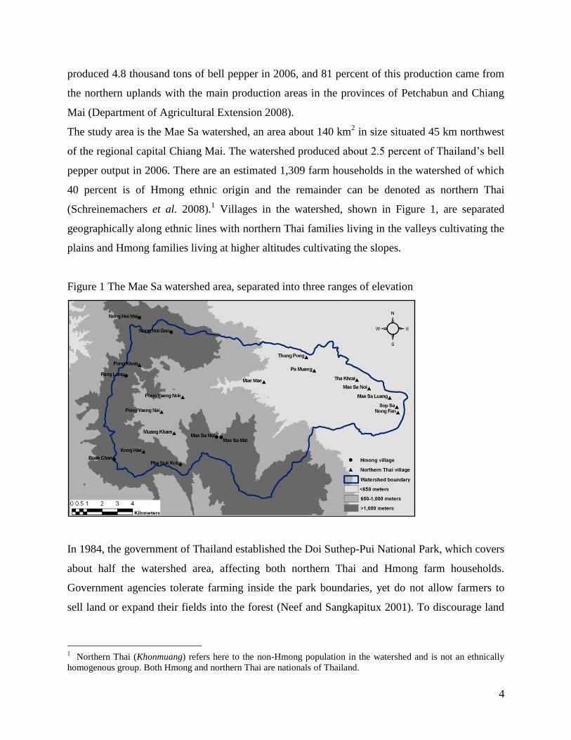
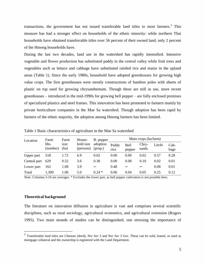
(Schreinemachers et al. 2008).1 Villages in the watershed, shown in Figure 1, are separated

geographically along ethnic lines with northern Thai families living in the valleys cultivating the

plains and Hmong families living at higher altitudes cultivating the slopes.

Figure 1 The Mae Sa watershed area, separated into three ranges of elevation

In 1984, the government of Thailand established the Doi Suthep-Pui National Park, which covers

about half the watershed area, affecting both northern Thai and Hmong farm households.

Government agencies tolerate farming inside the park boundaries, yet do not allow farmers to

sell land or expand their fields into the forest (Neef and Sangkapitux 2001). To discourage land

1 Northern Thai (Khonmuang) refers here to the non-Hmong population in the watershed and is not an ethnically

homogenous group. Both Hmong and northern Thai are nationals of Thailand.

5

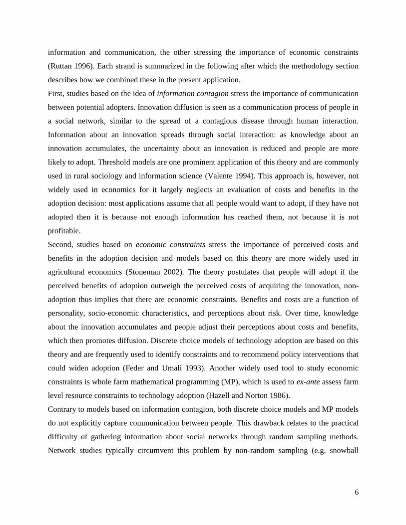
transactions, the government has not issued transferable land titles to most farmers.2 This

measure has had a stronger effect on households of the ethnic minority: while northern Thai

households have obtained transferrable titles over 56 percent of their owned land, only 2 percent

of the Hmong households have.

During the last two decades, land use in the watershed has rapidly intensified. Intensive

vegetable and flower production has substituted paddy in the central valley while fruit trees and

vegetables such as lettuce and cabbage have substituted rainfed rice and maize in the upland

areas (Table 1). Since the early 1980s, household have adopted greenhouses for growing high

value crops. The first greenhouses were mostly constructions of bamboo poles with sheets of

plastic on top used for growing chrysanthemum. Though these are still in use, more recent

greenhouses – introduced in the mid-1990s for growing bell pepper – are fully enclosed premises

of specialized plastics and steel frames. This innovation has been promoted to farmers mainly by

private horticulture companies in the Mae Sa watershed. Though adoption has been rapid by

farmers of the ethnic majority, the adoption among Hmong farmers has been limited.

Table 1 Basic characteristics of agriculture in the Mae Sa watershed

Location

Farm

hhs.

(number)

Farm size

(ha)

House-

hold size

(persons)

B. pepper

adoption

(prop.)

Main crops (ha/farm)

Paddy

rice Bell

pepper

Chry-

santh. Litchi

Cab-

bage

Upper part 518 1.72 6.9 0.02 0.00 0.00 0.02 0.57 0.28

Central part 629 0.52 3.6 0.38 0.00 0.08 0.10 0.02 0.01

Lower part 162 1.08 3.9 ─ 0.48 ─ ─ 0.08 0.01

Total 1,309 1.06 5.0 0.24 * 0.06 0.04 0.05 0.25 0.12

Note: Columns 3-10 are averages. * Excludes the lower part, as bell pepper cultivation is not possible here.

Theoretical background

The literature on innovation diffusion in agriculture is vast and comprises several scientific

disciplines, such as rural sociology, agricultural economics, and agricultural extension (Rogers

1995). Two main strands of studies can be distinguished, one stressing the importance of

2 Transferable land titles are Chanote (deed), Nor Sor 3 and Nor Sor 3 Gor. These can be sold, leased, or used as

mortgage collateral and the ownership is registered with the Land Department.

6

information and communication, the other stressing the importance of economic constraints

(Ruttan 1996). Each strand is summarized in the following after which the methodology section

describes how we combined these in the present application.

First, studies based on the idea of information contagion stress the importance of communication

between potential adopters. Innovation diffusion is seen as a communication process of people in

a social network, similar to the spread of a contagious disease through human interaction.

Information about an innovation spreads through social interaction: as knowledge about an

innovation accumulates, the uncertainty about an innovation is reduced and people are more

likely to adopt. Threshold models are one prominent application of this theory and are commonly

used in rural sociology and information science (Valente 1994). This approach is, however, not

widely used in economics for it largely neglects an evaluation of costs and benefits in the

adoption decision: most applications assume that all people would want to adopt, if they have not

adopted then it is because not enough information has reached them, not because it is not

profitable.

Second, studies based on economic constraints stress the importance of perceived costs and

benefits in the adoption decision and models based on this theory are more widely used in

agricultural economics (Stoneman 2002). The theory postulates that people will adopt if the

perceived benefits of adoption outweigh the perceived costs of acquiring the innovation, non-

adoption thus implies that there are economic constraints. Benefits and costs are a function of

personality, socio-economic characteristics, and perceptions about risk. Over time, knowledge

about the innovation accumulates and people adjust their perceptions about costs and benefits,

which then promotes diffusion. Discrete choice models of technology adoption are based on this

theory and are frequently used to identify constraints and to recommend policy interventions that

could widen adoption (Feder and Umali 1993). Another widely used tool to study economic

constraints is whole farm mathematical programming (MP), which is used to ex-ante assess farm

level resource constraints to technology adoption (Hazell and Norton 1986).

Contrary to models based on information contagion, both discrete choice models and MP models

do not explicitly capture communication between people. This drawback relates to the practical

difficulty of gathering information about social networks through random sampling methods.

Network studies typically circumvent this problem by non-random sampling (e.g. snowball

7

method) or surveying whole populations (Wasserman and Faust 1994), which is impractical in

large-scale surveys necessary for statistical analysis.

A second drawback of both discrete choice and MP models is that they do not well capture the

dynamics of innovation diffusion. Binary models estimated from cross-sectional data are

snapshots of the diffusion process, in which the regression parameters tend to be sensitive to the

adoption rate as the composition of the groups of non-adopters and adopters change over time as

people gradually move from the first to the latter. Moreover, binary models can only be

estimated on cross-sectional data if an innovation is relatively well-diffused. Aggregate MP

models based on representative farm households tend to give large jumps in optimum solutions

rather than the smooth S-shaped adoption curves that characterize innovation diffusion in reality.

In spite of each method‘s disadvantages, each also has its strengths in describing a particular

aspect of the innovation diffusion process. Threshold models highlight the aspect of

communication; discrete choice models highlight the aspect of constraints at village, regional, or

national levels, while MP models do so at the farm level, both ex ante and ex post. This paper

therefore shows how these approaches can be unified, thereby yielding new insights into the

dynamics of innovation diffusion in agriculture.

Methodology

Simulation models in general and agent-based models in particular are sometimes perceived as

black box models as it is difficult, if not impossible, to explain the whole ins and outs within the

length of a journal paper. This paper is therefore necessarily incomplete, as we describe only the

main components and main dynamics while the original MP-MAS model and extended

documentation is available online (http://mp-mas.uni-hohenheim.de). The emphasis in this

exposition lies on how we combined an econometrically estimated adoption function with an

agent-based model to simulate the diffusion of innovations under alternative scenarios.

Mathematical programming-based multi-agent systems (MP-MAS)

MP-MAS works with a set of input files that are organized in Microsoft Excel workbooks

(Berger and Schreinemachers 2009).3 It falls into a category of models called agent-based

3 MP-MAS is a freeware application developed at Hohenheim University. The software draws on the pioneering

work of Balmann (1997) that has been continued by Happe et al. (2006) as the AgriPolis model. The MP-MAS

8

models of land use and land cover change (ABM/LUCC). These models couple a cellular

component that represents a landscape with an agent-based component that represents human

decision-making (Parker et al. 2002). ABM/LUCC have been applied in a wide range of settings

(for overviews see: Janssen 2002, Parker et al. 2003) but have in common that agents are

autonomous decision-makers who interact and communicate and make decisions that can alter

the environment.

This application of MP-MAS to the diffusion of an agricultural innovation in northern Thailand

builds on previous applications of MP-MAS analyzing the diffusion of water-saving

technologies in an agricultural region in Chile (Berger 2001, Berger et al. 2007), and the

diffusion of high yielding maize varieties in two agricultural communities in southeast Uganda

(Berger et al. 2006, Schreinemachers 2006, Schreinemachers et al. 2007). This last application to

Uganda showed how MP-MAS can be parameterized from econometrically estimated production

and expenditure functions. The present study adds to this by showing how econometrically

estimated adoption functions can be used in MP-MAS to simulate the diffusion of innovations.

MP-MAS distinguishes itself most clearly from other ABM/LUCC in its use of well-established

methods in agricultural economics, such as agricultural production functions, household

expenditure models, binary adoption models, and mathematical programming (MP). In using

these methods, MP-MAS assumes that agents behave largely rational in their economic decision-

making about production and consumption. Many agent-based model applications have departed

from this assumption—stating that it is unrealistic—and have used decision-trees and condition-

action rules instead. In Schreinemachers and Berger (2006) we, however, argued that when

modeling complex farm-decisions, the disadvantages of rule-based decision systems might be

greater than the disadvantages of the rationality assumption. MP-MAS furthermore departs from

full economic foresight by explicitly including incomplete information and expectation

formation.

Agents and landscape

In MP-MAS, each farm household in the study area is represented as a single computational

agent in the model; hence, there are as many agents in the model as there are farm households in

software can be downloaded from http://mp-mas.uni-hohenheim.de. A detailed user manual is available from the

same website. MP-MAS is written in C++ programming language and is available for both Unix and Windows XP

operating systems.

9

reality. Agents own resources such as household labor, agricultural land, fruit orchards, and

greenhouses. The resource endowment of each agent was quantified from a random survey of a

quarter of all farm households in the study area. The sampling weights of the survey (the inverse

probability of selection) were used to multiply households inside the agent-based model. Each

farm household thus appeared about four times in the model. As the sampling fraction was high,

we judged this duplication as acceptable; otherwise we could have reverted to Monte Carlo

methods to increase the variation in the agent population as proposed in Berger and

Schreinemachers (2006).

The farm household decision-making of each agent is simulated by solving an MP tableau. One

generic MP tableau was specified for all agents while the MP-MAS software adjusts available

resources (i.e., right-hand-side values), technical coefficients, and other matrix coefficients for

each individual agent. The MP approach assumed farm households to maximize the expected net

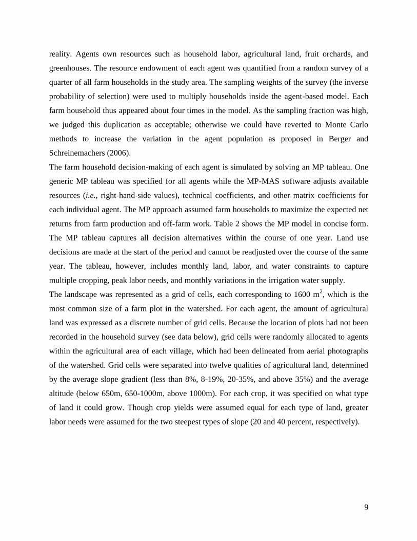
returns from farm production and off-farm work. Table 2 shows the MP model in concise form.

The MP tableau captures all decision alternatives within the course of one year. Land use

decisions are made at the start of the period and cannot be readjusted over the course of the same

year. The tableau, however, includes monthly land, labor, and water constraints to capture

multiple cropping, peak labor needs, and monthly variations in the irrigation water supply.

The landscape was represented as a grid of cells, each corresponding to 1600 m2, which is the

most common size of a farm plot in the watershed. For each agent, the amount of agricultural

land was expressed as a discrete number of grid cells. Because the location of plots had not been

recorded in the household survey (see data below), grid cells were randomly allocated to agents

within the agricultural area of each village, which had been delineated from aerial photographs

of the watershed. Grid cells were separated into twelve qualities of agricultural land, determined

by the average slope gradient (less than 8%, 8-19%, 20-35%, and above 35%) and the average

altitude (below 650m, 650-1000m, above 1000m). For each crop, it was specified on what type

of land it could grow. Though crop yields were assumed equal for each type of land, greater

labor needs were assumed for the two steepest types of slope (20 and 40 percent, respectively).

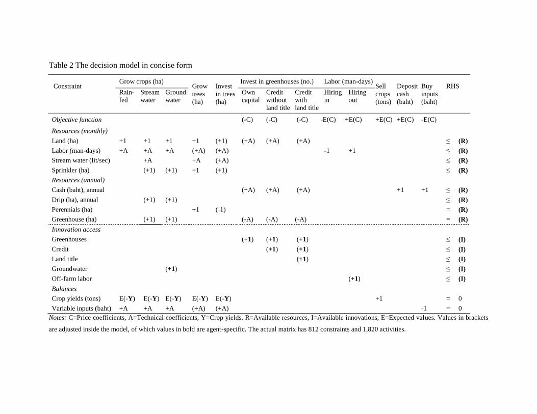
Table 2 The decision model in concise form

Constraint

Grow crops (ha) Grow

trees

(ha)

Invest

in trees

(ha)

Invest in greenhouses (no.) Labor (man-days) Sell

crops

(tons)

Deposit

cash

(baht)

Buy

inputs

(baht)

RHS

Rain-

fed

Stream

water

Ground

water

Own

capital

Credit

without

land title

Credit

with

land title

Hiring

in

Hiring

out

Objective function (-C) (-C) (-C) -E(C) +E(C) +E(C) +E(C) -E(C)

Resources (monthly)

Land (ha) +1 +1 +1 +1 (+1) (+A) (+A) (+A) ≤ (R)

Labor (man-days) +A +A +A (+A) (+A) -1 +1 ≤ (R)

Stream water (lit/sec) +A +A (+A) ≤ (R)

Sprinkler (ha) (+1) (+1) +1 (+1) ≤ (R)

Resources (annual)

Cash (baht), annual (+A) (+A) (+A) +1 +1 ≤ (R)

Drip (ha), annual (+1) (+1) ≤ (R)

Perennials (ha) +1 (-1) = (R)

Greenhouse (ha) (+1) (+1) (-A) (-A) (-A) = (R)

Innovation access

Greenhouses (+1) (+1) (+1) ≤ (I)

Credit (+1) (+1) ≤ (I)

Land title (+1) ≤ (I)

Groundwater (+1) ≤ (I)

Off-farm labor (+1) ≤ (I)

Balances

Crop yields (tons) E(-Y) E(-Y) E(-Y) E(-Y) E(-Y) +1 = 0

Variable inputs (baht) +A +A +A (+A) (+A) -1 = 0

Notes: C=Price coefficients, A=Technical coefficients, Y=Crop yields, R=Available resources, I=Available innovations, E=Expected values. Values in brackets

are adjusted inside the model, of which values in bold are agent-specific. The actual matrix has 812 constraints and 1,820 activities.

11

Dynamics of the model

Figure 2 shows the main dynamics in the model. For each year in the simulation, two MP

problems are solved for each agent, simulating investment and production decisions,

respectively. Investments include the acquisition of new technologies and assets, such as

greenhouses and fruit orchards, which have revenues over multiple years. For the investment

problem, which was solved first at the beginning of each simulation period, the agent optimized

the expected net returns averaged over the lifespan of each asset using an annuity cost approach.

For the following production problem, new investments were then added to the available

resources of the agent while the purchase price was subtracted from the agent‘s liquidity. This

second MP problem optimized the agent production decision: the allocation of cash, land, labor,

and water to a monthly cropping plan (Schreinemachers and Berger 2006 give more details on

this decision procedure).

Figure 2 Dynamics of the model

Notes: Investment and production decisions are simulated by optimizing the agent objective function subject to

constraints. Agents at this stage do not have complete information about output prices, crop yields, and the supply of

water, only expectations based on experience. The biophysical part of the MP-MAS model then simulates the supply

of water to each agent as based on rainfall and the flow of irrigation water in the watershed. Expected values are

then updated with simulated actual values to calculate the simulated actual farm performance (decision outcomes) at

the end of the year. Before entering the next simulation period, expectations and liquidity are updated for each agent

while the innovation diffusion model updates the access to innovations.

Investment decisions

Production decisions

Decision outcomes

Rainfall & inflows

Crop yields

Updating of expectations (prices, yields, water supply) and liquidity Evaluation of innovation thresholds

Simulated by solving MP tableaus for each agent

Updating of liquidity & assets

12

Investment and production decisions are both based on expected values for prices, crop yields,

rainfall, and irrigation water supply and are based on the theory of adaptive expectations (Arrow

and Nerlove 1958). This theory entails that people form expectations about what will happen in

the future based on what happened in the past. The theory is only realistic if there is no

systematic trend that real decision-makers could learn from and use to adjust their expectations

(that is, to develop foresight). Following the implementation of adaptive expectations in MP-

MAS by Berger (2001), agents revise their expectations in each period in proportion to the

difference between actual (Xt-1) and expected values (X*t-1) as:

X*t =

X

*t-1+ λ * [Xt-1 – X

*t-1], 0 < λ ≤ 1 (1)

in which λ is the coefficient of expectations.

After agents decide on investment and production, the solution vector of the MP matrix is

recalculated for each agent using actual values. Prices, rainfall, and the total irrigation water

supply are exogenous to the agent decisions and are specified in the model input data. Crop

yields are simulated as a function of the actual water supply as explained below.

The revenues from farm production and off-farm work are partly consumed and partly added to

the agents‘ assets in the form of savings, which can be used in the next period for investment and

production. Based on the obtained prices, crop yields, and water supply, agents update their

expectations for the next period.

Innovation diffusion

Innovativeness is generally seen as a personal characteristic that varies among farm households.

The most innovative farmers are risk-taking—easily trying new technologies, while less

innovative farmers are more risk-averse—only considering adoption if many peers have

successfully adopted already. Rogers (1995) divided the population of potential adopters into

five groups: innovators (the most innovative 2.5%), early adopters (2.5-16%), early majority (16-

50%), late majority (50-84%), and laggards (remaining 16%). MP-MAS follows this approach

by dividing the agent population into five groups.

Because the level of innovativeness of a farm household cannot directly be recorded by means of

a farm household survey, we used a binary adoption model to predict a probability of adoption

from a set of observable independent variables, assuming that a higher predicted probability of

13

adoption is associated with a higher innovativeness of a household. The random sample of

households has no selection bias stemming from non-exposure as all farm households in the

study area know about greenhouses; adoption was therefore modeled as a single equation in

which the dependent variable (greenhouse adoption) was either one (farm household did adopt)

or zero (did not adopt). We assumed a cumulative logistic probability function, in which the

probability of adoption (Pk) is a function of a set of independent variables (Xk):

(2)

with e being the base of the natural logarithm. Pk can be approximated as rk/nk where rk is the

number of times the first alternative is chosen by the household k with a given Xk, and nk is the

total number of households having a given Xk. The probability model can be made linear in the

parameters by a logarithmic transformation:

(3)

As independent variables were used:

The amount of agricultural land and the percentage of on-farm work in total labor supply

both indicating a commitment to farming and were expected to have a positive effect on

adoption.

The slope gradient of agricultural land was included as a dummy, being zero if less than half

the land was flat. Sloping areas were expected to hamper adoption because of more extensive

needs of landscaping that increase investment costs.

Transferable land titles were also included as a dummy, defaulting to zero if less than half

the agricultural land owned by the household had no transferable title.

Since greenhouses are capital intensive, they generally require credit. Access to credit was

approximated as a dummy with the value of one if the household received a credit in the

previous 12 months.

Greenhouse agriculture is also capital intensive and requires special skills; farm households

who have received formal education might be better positioned to acquire these skills. A

dummy variable was included and was expected to have a positive sign.

Lastly, to control for the effect of ethnicity, a dummy for Hmong households was included.

14

Because greenhouses are only suitable for areas at an elevation 500 meters a.s.l. and above, the

population of potential adopters was smaller than the total population of farm households. In the

model, agents with plots at lower altitudes were therefore not given access to this innovation. As

the study area is small and road infrastructure is relatively good throughout the watershed,

distance measures to markets or roads were not included.

Sample households were ranked by their predicted probability of adoption, as estimated from the

logit model, and divided into five innovator groups following the classification of Rogers (1995).

The upper boundary of each group was taken as a threshold value for the next group; hence,

adoption in more innovative groups needs to be complete before less innovative groups can start

adopting. For instance, an agent belonging to the group of early adopters (threshold value 16%),

can only adopt the innovation after adoption in the whole population has breached the 16%

threshold. As about a quarter of all households in the upper and central part of the watershed

have adopted greenhouses, it was assumed that the first three segments had access to the

innovation, while the late majority and laggard segment are still postponing their decision until

the early majority has completed adoption.

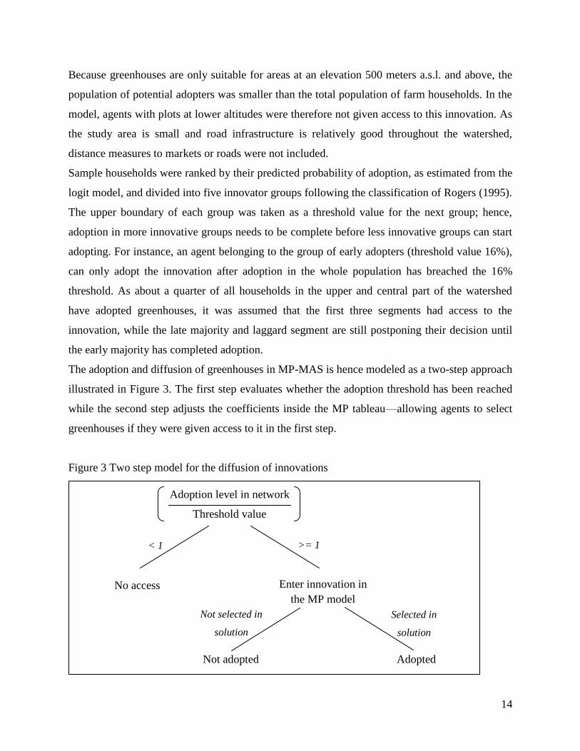
The adoption and diffusion of greenhouses in MP-MAS is hence modeled as a two-step approach

illustrated in Figure 3. The first step evaluates whether the adoption threshold has been reached

while the second step adjusts the coefficients inside the MP tableau—allowing agents to select

greenhouses if they were given access to it in the first step.

Figure 3 Two step model for the diffusion of innovations

Enter innovation in

the MP model

No access

< 1 >= 1

Selected in

solution

Not adopted Adopted

Not selected in

solution

Adoption level in network

Threshold value

15

Solving the investment problem then simulates the actual adoption decision of the agents. An

increase in the adoption rate would make the innovation available to further adopter groups in

the next year of the simulation. The interaction between agents in the model is hence

implemented indirectly as a frequency-dependent effect: agents monitor the adoption rate in the

population and compare this to their personal willingness to take risk.

An additional purpose of the logit model was to identify economic constraints to greenhouse

adoption. The identified constraints were used in the design of the MP tableau: greenhouse

activities were specified for land with and without secure titles and for various slope positions.

Crop water demand and crop yield

Crop yields were modeled following the FAO CropWat model (Smith 1992, Clarke et al. 1998).

The crop-water requirement (CWR) for crop c in month m is the product of a crop coefficient

(Kc), the potential evapotranspiration (ETO), and the planted area (Area):

CWRcm = Kccm* ETOm * Areacm (4)

The CWR could either be met through irrigation (IRR) or rainfall, which was converted into

effective rainfall (ER) to capture the share of rainfall actually available to the crop, depending on

its growth stage. The amount of water actually supplied (CWS) was then as follows:

CWScm = ERcm + IRRcm (5)

For lack of detailed data from the study region, the quotient of crop water supplied and the crop

water requirement were simply averaged over all months with non-zero crop water requirements:

Krc = (1/m * ∑(CWScm / CWRcm) | CWRcm > 0) (6)

The crop growth model assumed that the crop yield was lost if the average Kr fell below 0.5,

while for Kr values greater than or equal to 0.5 the Kr value was multiplied by the crop yield

potential (YPOT) to simulate the actual crop yield (Yc):

(7)

Crop water supply

Rainfall, groundwater, and surface water are the sources of crop water supply in the model. Daily

rainfall data were generated in two steps following Yaoming et al. (2004). In the first step, a first

Yc =

Krc * YPOTc if Krc ≥ 0.5

0 if Krc < 0.5

16

order Markov chain was used to simulate discrete rainfall events (wet or dry days), while in the

second step a two parameter gamma distribution was used to simulate the rainfall amounts on

wet days. The parameters of the gamma distribution were estimated by fitting it to historical

rainfall data. The daily simulated rainfall amounts were summed to monthly amounts and entered

into the model.

Agents, as their real-world analogues, derive irrigation water from either groundwater or streams

(surface water). In the study area, groundwater pumping is currently only possible in the

watershed‘s valley where it is used to irrigate about 11 percent of the agricultural area, mostly

under greenhouses. The model assumed that agents who already had access to groundwater had

an unlimited supply to irrigate their greenhouses, while other agents could not install new pumps.

While groundwater was assumed to give an unlimited water supply, surface water needed to be

shared among agents in the same village. The irrigation water supply (IRR in equation 5) is

difficult to measure in the field but can be approximated using a backward calculation of the

irrigation requirements based on an observed pattern of land use, irrigation methods, irrigation

sources, and effective rainfall. Let IEFFjck be the efficiency of irrigation method j used on crop c

by a household k. The irrigation water use of household k was then calculated by summing the

irrigation water use over all months and crops as:

IRRk = ∑m ∑c (CWRckm – ERm – GRmc) * IEFFjck (8)

in which GR was the groundwater supply. The sum over all households in an area that shared a

common water source thereby approximated the total volume of the surface water for irrigation.

The household‘s share in the total water supply was used to approximate the agents‘ water rights

in the model. This water right was assumed constant over the simulation horizon and was used to

calculate the agents‘ irrigation water supply in each month and in each period of the simulation.

Outcome indicators

Four outcome indicators were used to analyze the simulation results. Economic indicators

included the greenhouse adoption rate and the net household incomes. Biophysical indicators

included irrigation water use and pesticide load. Pesticide load was quantified using the

Environmental Impact Quotient method (Kovach et al. 2008). Following this method, an average

field use rating, a proxy for toxicity, was calculated for each crop. The field use rating is the

product of three factors: the proportion of active ingredient in a pesticide, the average application

rate of the pesticide on a crop, and an EIQ factor reflecting the toxicity of the pesticide to farm

17

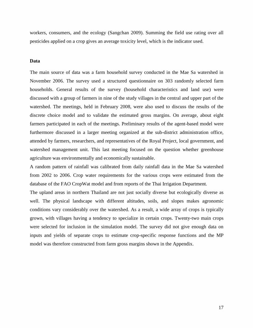
workers, consumers, and the ecology (Sangchan 2009). Summing the field use rating over all

pesticides applied on a crop gives an average toxicity level, which is the indicator used.

Data

The main source of data was a farm household survey conducted in the Mae Sa watershed in

November 2006. The survey used a structured questionnaire on 303 randomly selected farm

households. General results of the survey (household characteristics and land use) were

discussed with a group of farmers in nine of the study villages in the central and upper part of the

watershed. The meetings, held in February 2008, were also used to discuss the results of the

discrete choice model and to validate the estimated gross margins. On average, about eight

farmers participated in each of the meetings. Preliminary results of the agent-based model were

furthermore discussed in a larger meeting organized at the sub-district administration office,

attended by farmers, researchers, and representatives of the Royal Project, local government, and

watershed management unit. This last meeting focused on the question whether greenhouse

agriculture was environmentally and economically sustainable.

A random pattern of rainfall was calibrated from daily rainfall data in the Mae Sa watershed

from 2002 to 2006. Crop water requirements for the various crops were estimated from the

database of the FAO CropWat model and from reports of the Thai Irrigation Department.

The upland areas in northern Thailand are not just socially diverse but ecologically diverse as

well. The physical landscape with different altitudes, soils, and slopes makes agronomic

conditions vary considerably over the watershed. As a result, a wide array of crops is typically

grown, with villages having a tendency to specialize in certain crops. Twenty-two main crops

were selected for inclusion in the simulation model. The survey did not give enough data on

inputs and yields of separate crops to estimate crop-specific response functions and the MP

model was therefore constructed from farm gross margins shown in the Appendix.

18

Results

Constraints to greenhouse adoption

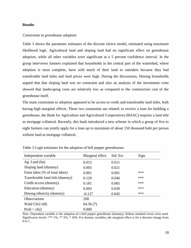
Table 3 shows the parameter estimates of the discrete choice model, estimated using maximum

likelihood logit. Agricultural land and sloping land had no significant effect on greenhouse

adoption, while all other variables were significant at a 5 percent confidence interval. In the

group interviews farmers explained that households in the central part of the watershed, where

adoption is most complete, have sold much of their land to outsiders because they had

transferable land titles and land prices were high. During the discussions, Hmong households

argued that that sloping land was no constraint and also an analysis of the investment costs

showed that landscaping costs are relatively low as compared to the construction cost of the

greenhouse itself.

The main constraints to adoption appeared to be access to credit and transferable land titles, both

having high marginal effects. These two constraints are related: to receive a loan for building a

greenhouse, the Bank for Agriculture and Agricultural Cooperatives (BAAC) requires a land title

as mortgage collateral. Recently, this bank introduced a new scheme in which a group of five to

eight farmers can jointly apply for a loan up to maximum of about 150 thousand baht per person

without land as mortgage collateral.

Table 3 Logit estimates for the adoption of bell pepper greenhouses

Independent variable Marginal effect Std. Err. Sign.

Ag. Land (ha) 0.015 0.011

Sloping land (dummy) 0.003 0.021

Farm labor (% of total labor) 0.001 0.001 ***

Transferable land title (dummy) 0.120 0.046 ***

Credit access (dummy) 0.181 0.065 ***

Education (dummy) 0.093 0.030 ***

Hmong ethnicity (dummy) -0.127 0.045 ***

Observations 268

Wald Chi2 (df) 64.36 (7)

Prob > chi2 0.000

Note: Dependent variable is the adoption of a bell pepper greenhouse (dummy). Robust standard errors were used.

Significance levels: *** 1%, ** 5%, * 10%. For dummy variables, the marginal effect is for a discrete change from

0 to 1.

19

The results suggest that, controlling for all other factors, access to credit would increase the

probability of adoption by 18 percent while a hypothetical switch to transferable land titles

would increase the probability of adoption by 12 percent. Because both variables are

conceptually related, one could expect multicollinearity in the estimation. The variance inflation

factors for both variables were, however, below 2—suggesting that multicollinearity might not

be an issue here.

Though the model predicts access to credit to increase greenhouse adoption, as a comparative

static model that lacks system dynamics it does not predict when this adoption would occur. This

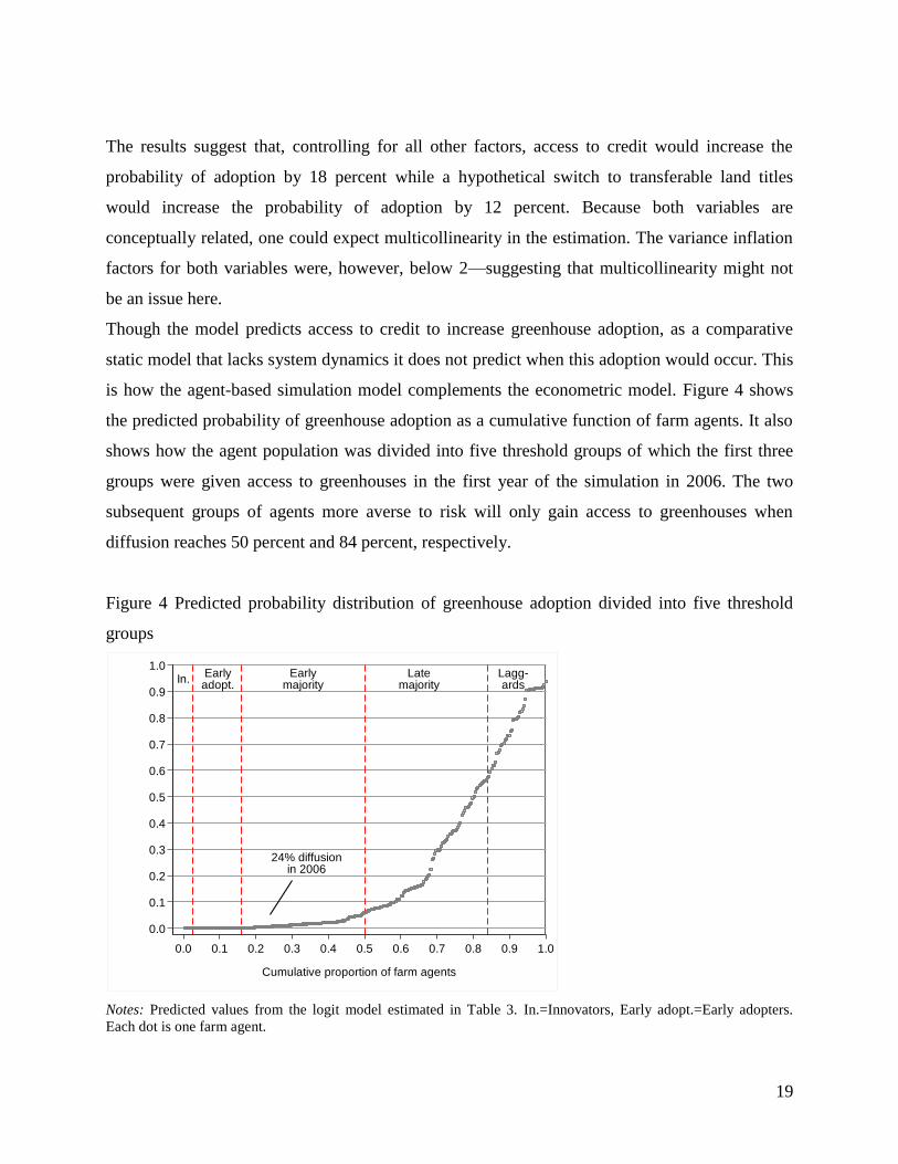
is how the agent-based simulation model complements the econometric model. Figure 4 shows

the predicted probability of greenhouse adoption as a cumulative function of farm agents. It also

shows how the agent population was divided into five threshold groups of which the first three

groups were given access to greenhouses in the first year of the simulation in 2006. The two

subsequent groups of agents more averse to risk will only gain access to greenhouses when

diffusion reaches 50 percent and 84 percent, respectively.

Figure 4 Predicted probability distribution of greenhouse adoption divided into five threshold

groups

Notes: Predicted values from the logit model estimated in Table 3. In.=Innovators, Early adopt.=Early adopters.

Each dot is one farm agent.

In.Earlyadopt.

Earlymajority

Latemajority

Lagg-ards

24% diffusionin 2006

0.0

0.1

0.2

0.3

0.4

0.5

0.6

0.7

0.8

0.9

1.0

Pre

dic

ted

pro

ba

bili

ty o

f a

do

ptio

n

0.0 0.1 0.2 0.3 0.4 0.5 0.6 0.7 0.8 0.9 1.0

Cumulative proportion of farm agents

20

Validation of the agent-based model

Validation of spatial simulation models and especially agent-based models is a much debated

topic in the literature (Pontius and Schneider 2001, Parker et al. 2003). The challenge is,

however, not specific to agent-based models but applies to complex models in general. Janssen

and van Ittersum (2007), for instance, reviewed 48 bio-economic farm models and found that

only 23 studies validated their results while only four did so quantitatively.

In econometric models, the difference between predicted and observed values is commonly used

as a measure of goodness-of-fit of a model; more precisely, the R2 measures how much of the

observed variation in the dependent variable could be explained by the model. Whole farm

programming models are often validated in a similar way, by plotting the predicted and observed

land use and fitting a regression line through the origin (McCarl and Apland 1986). Because the

agent-based model was based on individual programming models, this method could be used for

model validation in this study. We note that, in a strict sense, this approach is only an ―informal‖

validation because the simulated and observed data are not independent.

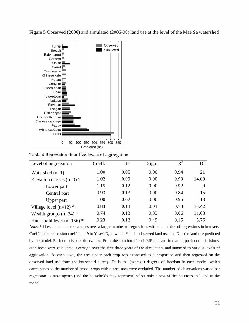
The comparison of observed and predicted values was done at various levels of aggregation,

from the watershed level to the household level. Figure 5 compares the observed land use with

the predicted land use at the watershed level. The fit between observed and predicted values is

relatively good for most crops. About 150 ha of cropland are, however, under crops not captured

in the model.

To quantify the fit each crop was expressed as a percentage of the total area under crops,

including only crops captured in the model. A regression line through the origin was then fitted

between the two variables. As the eight lowland villages have only few farmers these were

grouped into two villages, giving a total of 12 villages in the whole watershed. To get one level

of aggregation between the village and the household level, farm households in each village were

sorted by their initial amount of liquid means, which was taken as a proxy of wealth, and dived

into three equal ―wealth groups‖, which gave 36 groups in total. At each level of aggregation,

regression lines were only estimated if more than two crops were grown, which reduced the

number of observations at the lower levels of aggregation. Table 4 shows the results.

21

Figure 5 Observed (2006) and simulated (2006-08) land use at the level of the Mae Sa watershed

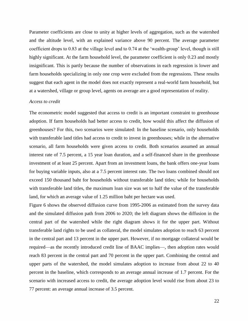
Table 4 Regression fit at five levels of aggregation

Level of aggregation Coeff. SE Sign. R2 Df

Watershed (n=1) 1.00 0.05 0.00 0.94 21

Elevation classes (n=3) * 1.02 0.09 0.00 0.90 14.00

Lower part 1.15 0.12 0.00 0.92 9

Central part 0.93 0.13 0.00 0.84 15

Upper part 1.00 0.02 0.00 0.95 18

Village level (n=12) * 0.83 0.13 0.01 0.73 13.42

Wealth groups (n=34) * 0.74 0.13 0.03 0.66 11.03

Household level (n=156) * 0.23 0.12 0.49 0.15 5.76

Note: * These numbers are averages over a larger number of regressions with the number of regressions in brackets.

Coeff. is the regression coefficient b in Y=a+bX, in which Y is the observed land use and X is the land use predicted

by the model. Each crop is one observation. From the solution of each MP tableau simulating production decisions,

crop areas were calculated, averaged over the first three years of the simulation, and summed to various levels of

aggregation. At each level, the area under each crop was expressed as a proportion and then regressed on the

observed land use from the household survey. Df is the (average) degrees of freedom in each model, which

corresponds to the number of crops; crops with a zero area were excluded. The number of observations varied per

regression as most agents (and the households they represent) select only a few of the 23 crops included in the

model.

0 50 100 150 200 250 300 350

Crop area (ha)

Litchi

White cabbage

Paddy

Chinese cabbage

Chrysanthemum

Bell pepper

Longan

Soybean

Lettuce

Sweetcorn

Rose

Green bean

Chayote

Potato

Chinese kale

Feed maize

Carrot

Onion

Gerbera

Baby carrot

Brocoli

Turnip Observed

Simulated

22

Parameter coefficients are close to unity at higher levels of aggregation, such as the watershed

and the altitude level, with an explained variance above 90 percent. The average parameter

coefficient drops to 0.83 at the village level and to 0.74 at the ‗wealth-group‘ level, though is still

highly significant. At the farm household level, the parameter coefficient is only 0.23 and mostly

insignificant. This is partly because the number of observations in each regression is lower and

farm households specializing in only one crop were excluded from the regressions. These results

suggest that each agent in the model does not exactly represent a real-world farm household, but

at a watershed, village or group level, agents on average are a good representation of reality.

Access to credit

The econometric model suggested that access to credit is an important constraint to greenhouse

adoption. If farm households had better access to credit, how would this affect the diffusion of

greenhouses? For this, two scenarios were simulated: In the baseline scenario, only households

with transferable land titles had access to credit to invest in greenhouses; while in the alternative

scenario, all farm households were given access to credit. Both scenarios assumed an annual

interest rate of 7.5 percent, a 15 year loan duration, and a self-financed share in the greenhouse

investment of at least 25 percent. Apart from an investment loans, the bank offers one-year loans

for buying variable inputs, also at a 7.5 percent interest rate. The two loans combined should not

exceed 150 thousand baht for households without transferable land titles; while for households

with transferable land titles, the maximum loan size was set to half the value of the transferable

land, for which an average value of 1.25 million baht per hectare was used.

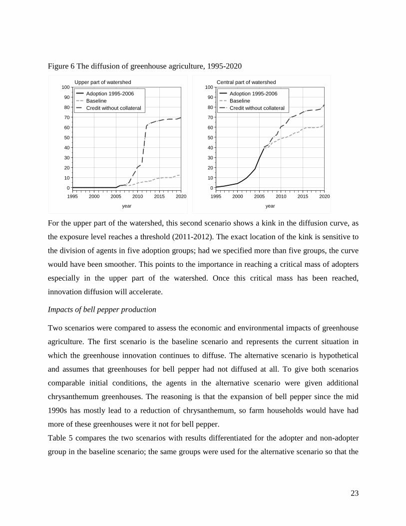
Figure 6 shows the observed diffusion curve from 1995-2006 as estimated from the survey data

and the simulated diffusion path from 2006 to 2020; the left diagram shows the diffusion in the

central part of the watershed while the right diagram shows it for the upper part. Without

transferable land rights to be used as collateral, the model simulates adoption to reach 63 percent

in the central part and 13 percent in the upper part. However, if no mortgage collateral would be

required—as the recently introduced credit line of BAAC implies—, then adoption rates would

reach 83 percent in the central part and 70 percent in the upper part. Combining the central and

upper parts of the watershed, the model simulates adoption to increase from about 22 to 40

percent in the baseline, which corresponds to an average annual increase of 1.7 percent. For the

scenario with increased access to credit, the average adoption level would rise from about 23 to

77 percent: an average annual increase of 3.5 percent.

23

Figure 6 The diffusion of greenhouse agriculture, 1995-2020

For the upper part of the watershed, this second scenario shows a kink in the diffusion curve, as

the exposure level reaches a threshold (2011-2012). The exact location of the kink is sensitive to

the division of agents in five adoption groups; had we specified more than five groups, the curve

would have been smoother. This points to the importance in reaching a critical mass of adopters

especially in the upper part of the watershed. Once this critical mass has been reached,

innovation diffusion will accelerate.

Impacts of bell pepper production

Two scenarios were compared to assess the economic and environmental impacts of greenhouse

agriculture. The first scenario is the baseline scenario and represents the current situation in

which the greenhouse innovation continues to diffuse. The alternative scenario is hypothetical

and assumes that greenhouses for bell pepper had not diffused at all. To give both scenarios

comparable initial conditions, the agents in the alternative scenario were given additional

chrysanthemum greenhouses. The reasoning is that the expansion of bell pepper since the mid

1990s has mostly lead to a reduction of chrysanthemum, so farm households would have had

more of these greenhouses were it not for bell pepper.

Table 5 compares the two scenarios with results differentiated for the adopter and non-adopter

group in the baseline scenario; the same groups were used for the alternative scenario so that the

Upper part of watershed

0

10

20

30

40

50

60

70

80

90

100

perc

enta

ge

1995 2000 2005 2010 2015 2020

year

Adoption 1995-2006

Baseline

Credit without collateral

Central part of watershed

0

10

20

30

40

50

60

70

80

90

100

perc

enta

ge

1995 2000 2005 2010 2015 2020

year

Adoption 1995-2006

Baseline

Credit without collateral

24

numbers for both scenarios refer to the same agents. Differences between the two scenarios were

compared using a t-test for paired data.

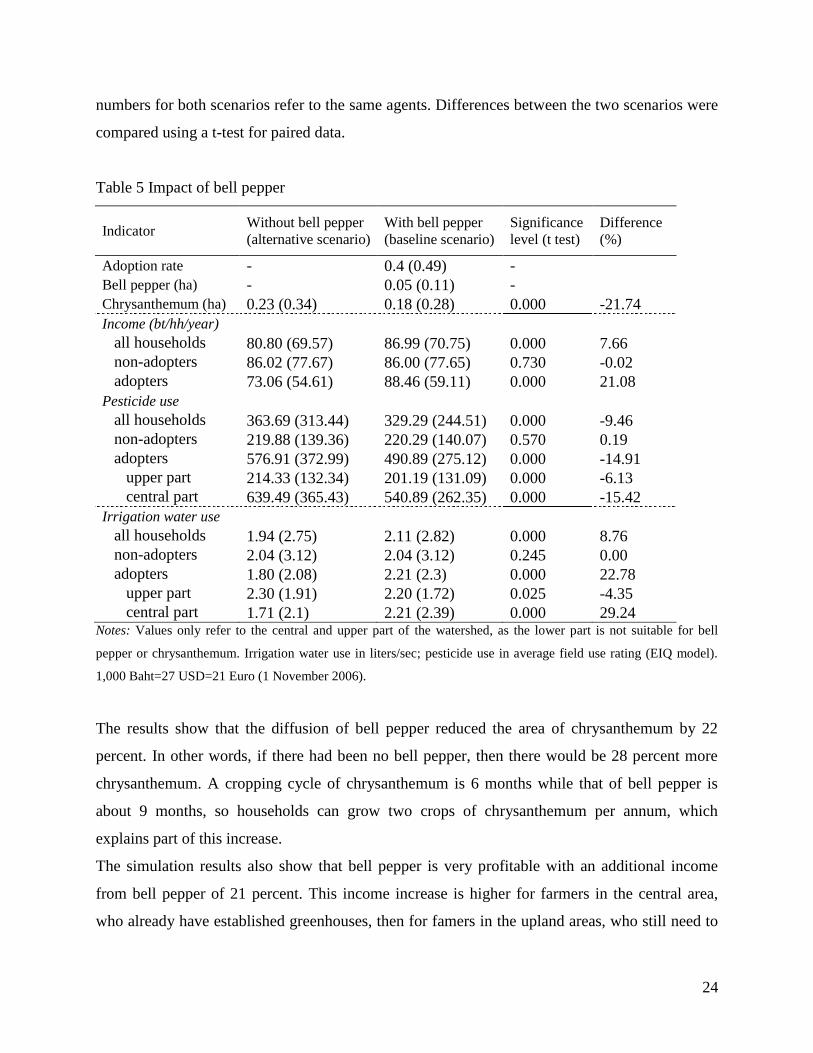
Table 5 Impact of bell pepper

Indicator Without bell pepper (alternative scenario)

With bell pepper

(baseline scenario) Significance

level (t test) Difference

(%)

Adoption rate - 0.4 (0.49) -

Bell pepper (ha) - 0.05 (0.11) -

Chrysanthemum (ha) 0.23 (0.34) 0.18 (0.28) 0.000 -21.74

Income (bt/hh/year)

all households 80.80 (69.57) 86.99 (70.75) 0.000 7.66

non-adopters 86.02 (77.67) 86.00 (77.65) 0.730 -0.02

adopters 73.06 (54.61) 88.46 (59.11) 0.000 21.08

Pesticide use

all households 363.69 (313.44) 329.29 (244.51) 0.000 -9.46

non-adopters 219.88 (139.36) 220.29 (140.07) 0.570 0.19

adopters 576.91 (372.99) 490.89 (275.12) 0.000 -14.91

upper part 214.33 (132.34) 201.19 (131.09) 0.000 -6.13

central part 639.49 (365.43) 540.89 (262.35) 0.000 -15.42

Irrigation water use

all households 1.94 (2.75) 2.11 (2.82) 0.000 8.76

non-adopters 2.04 (3.12) 2.04 (3.12) 0.245 0.00

adopters 1.80 (2.08) 2.21 (2.3) 0.000 22.78

upper part 2.30 (1.91) 2.20 (1.72) 0.025 -4.35

central part 1.71 (2.1) 2.21 (2.39) 0.000 29.24 Notes: Values only refer to the central and upper part of the watershed, as the lower part is not suitable for bell

pepper or chrysanthemum. Irrigation water use in liters/sec; pesticide use in average field use rating (EIQ model).

1,000 Baht=27 USD=21 Euro (1 November 2006).

The results show that the diffusion of bell pepper reduced the area of chrysanthemum by 22

percent. In other words, if there had been no bell pepper, then there would be 28 percent more

chrysanthemum. A cropping cycle of chrysanthemum is 6 months while that of bell pepper is

about 9 months, so households can grow two crops of chrysanthemum per annum, which

explains part of this increase.

The simulation results also show that bell pepper is very profitable with an additional income

from bell pepper of 21 percent. This income increase is higher for farmers in the central area,

who already have established greenhouses, then for famers in the upland areas, who still need to

25

pay investment costs. We also note that a greater chrysanthemum output could have depressed

output prices for this flower and have exposed farmers to greater yield and price risks.

The results suggest that the pesticide load for the watershed as a whole is 15 percent lower in the

scenario with bell pepper than in the scenario without bell pepper. Chrysanthemum requires

fewer pesticides per cropping cycle than bell pepper, but because of multiple cropping, the

average pesticide load per hectare is greater. This finding contradicts the common perception that

bell pepper has increased pesticide loads: the effect on pesticide load depends on the pest

management in the crop that was replaced; hence the effect is much larger in the central part—

where it replaced chrysanthemum, than in the upper part—where it is replacing litchi and

vegetables. We note, however, that the average level of pesticide use of adopting farm

households is more than double that of non-adopting households in both scenarios, hence the

cultivation of both bell pepper and chrysanthemum is relatively polluting.

Finally, concerning irrigation water use, the results show that bell pepper does intensify

irrigation water needs on average, though also here the effect is larger in the central part—where

it leads to an increase in groundwater pumping, than in the upper part—where water is

constrained and water is therefore diverted from other crops. The irrigation needs of bell pepper

adopters are on average 23 percent greater than in the scenario without bell pepper adoption.

Discussion

The diffusion of agricultural innovations is an example of complex system behavior: from the

individual decisions and interactions of single farm households an aggregate pattern of

innovation diffusion emerges, a pattern that could not have been predicted by the observation of

individual behavior in isolation. The paper demonstrated that such complex system behavior can

be simulated by combining conventional modeling such as mathematical programming, discrete

choice, and threshold models in an agent-based simulation approach. While the agent-based

model does not accurately represent the decisions of individual real-world farm households, the

validation exercise suggested a good model fit at levels of aggregation above the individual farm

household.

The disaggregated modeling approach allows taking into account the heterogeneity of and

interaction between farm households. To exploit the advantages of our agent-based approach

further, more interactions—for instance, as shown in Berger (2001) and Berger et al. (2007)—

26

will be included in future versions of the model. Such interactions can, for example, include the

buying and selling of agricultural land, the negotiation about local water rights, and informal

labor markets. For the current assessment of greenhouse diffusion, we judged that not including

these aspects is an acceptable simplification of reality.

The study showed that farm households in the Mae Sa watershed are constrained in the adoption

of greenhouses for bell pepper by their limited access to credit. Lack of transferable land titles

has prevented especially Hmong farm households, living in the upper parts of the watershed,

from obtaining commercial loans. The simulation results suggested that if mortgage collateral

would not be required, as was recently introduced by BAAC, then this would increase the

adoption of greenhouses for bell pepper to nearly 70 percent in the upper part and to nearly 83

percent in the central part by 2020. These results are, however, based on a number of

assumptions, some of which we will discuss in the following.

Two uncertain variables in the agent-based model are the initial amounts of liquidity and the

supply of irrigation water. Both were quantified based on the observed pattern of land use, as

direct measurement was not possible. The actual availability of liquidity and irrigation water

might, however, be greater than what was entered in the model. Because the study showed

liquidity to constrain the adoption of greenhouses, the simulation results are likely to be sensitive

to this variable. More study is therefore needed to test the sensitivity of our findings to

alternative assumption about liquidity and irrigation water.

A further limitation of the present model derives from the use of gross margins, which are fixed

combinations of inputs and outputs. The number of crops was too large to collect detailed

production data to estimate continuous production functions for each crop. The drawback for the

agent-based model is that it limits the heterogeneity in simulation outcomes. Agents, as the farm

households they represent, face different scarcity conditions in their inputs, as they possess

different amounts of land, labor, and cash; it is therefore unrealistic to assume that they all

produce at the same point in the production function. However, the choice between crops still

allows the agents to some degree to tailor their land use to the individual scarcity conditions.

Another critical assumption was that of constant prices. Bell pepper prices are unlikely to remain

at current levels and during the group meetings, farmers complained that selling prices has gone

down, while the cost of especially fertilizers has gone up. Farmers know that market supply

27

needs to be reduced by discarding low-grade products, yet this has been difficult to do in practice

as each farmer has an incentive to maximize returns.

Concerning the environmental impact of greenhouses for bell pepper, the results were mixed.

The simulation results showed a greater average irrigation water use yet a lower pesticide use. As

compared to chrysanthemum, bell pepper uses fewer pesticides per hectare and per year. Yet,

average pesticide field use ratings for both crops are extremely high, so that this positive effect

of bell pepper should not be overstated.

Whether greenhouses for bell pepper in the Mae Sa watershed are economically efficient and

environmentally sustainable has not been answered by this study. Farmers who have grown bell

pepper for many years reported difficulties controlling pests and fungi. Some farmers, unable to

control pests, took the drastic decision to break down their greenhouses in the watershed and

build them up again elsewhere. Alternating bell pepper with tomato or cucumber gives low

returns, as current market prices for these alternating crops are low. Insufficient knowledge with

the innovation seems to be a main problem. Surveying 46 plots of bell pepper, we found 55

different types of pesticides, herbicides, and fungicides applied. Farmers admitted difficulties in

choosing the right kind of pesticides and the right method of using them. Farmers tend to throw

away infected plants just outside their greenhouse instead of properly discarding them.

Efficiency gains in bell pepper production are therefore possible and increased market

competition is likely to create incentives for some farmers to become more efficient, while others

might have to give up bell pepper growing. During the meetings in the study villages, we asked

farmers for their opinion about the future of greenhouse agriculture. While Hmong farmers

showed a certain urgency to adopt or expand greenhouses as long as prices are high, northern

Thai farmers were more pessimistic and some thought that bell pepper could disappear within the

next five years if pests cannot be controlled. Research and extension will therefore be needed to

improve both the economic and environmental sustainability of greenhouse farming.

Conclusion

Farm households in the Mae Sa watershed who have not been issued transferable land titles have

difficulties raising enough cash to invest into greenhouses. This has especially prevented farm

households from the Hmong ethnic minority in the upper parts of the watershed from adopting

the innovation. If mortgage collateral would not be required, then this could increase the

28

adoption to nearly 70 percent in the upper part and to nearly 83 percent in the central part of the

watershed by 2020. Greenhouses for bell pepper have had a significant and positive effect on

average incomes. Pesticide loads, though still high, are lower with bell pepper than with the

alternative of chrysanthemum. Yet, the innovation has increased the needs for irrigation water.

Acknowledgement

Financial support of the Deutsche Forschungsgemeinschaft (DFG) under SFB-564 is gratefully

acknowledged. We thank Tanaporn Hunkittikul and Orn-uma Polpanich for their research

assistance and we thank Cindy Hugenschmidt and Walaya Sangchan for sharing data with us.

We are grateful to two anonymous reviewers of this journal for their comments.

References

Arrow, K. J. and Nerlove, M. 1958. A Note on Expectations and Stability. Econometrica, 26(2):

297-305.

Balmann, A. 1997. Farm-based Modelling of Regional Structural Change: A Cellular Automata

Approach. European Review of Agricultural Economics, 24: 85-108.

Berger, T. 2001. Agent-based models applied to agriculture: a simulation tool for technology

diffusion, resource use changes and policy analysis. Agricultural Economics, 25(2/3):

245-260.

Berger, T. and Schreinemachers, P. 2006. Creating agents and landscapes for multiagent systems

from random samples. Ecology and Society, 11(2): Art.19.

Berger, T., Birner, R., Díaz, J., McCarthy, N., and Wittmer, H., 2007. Capturing the complexity

of water uses and water users within a multi-agent framework. Water Resources Manage-

ment, 21: 129–148.

Berger, T. and Schreinemachers, P. 2009. Mathematical programming-based multi-agent

systems (MP-MAS). Technical model documentation. Version 2.0, February 2009,.

Stuttgart: Hohenheim University.

Berger, T., Schreinemachers, P., and Woelcke, J., 2006. Multi-agent simulation for development

of less-favored areas. Agricultural Systems, 88: 28-43.

Clarke, D., Smith, M., and El-Askari, K. 1998. CropWat for Windows: User Guide, University

of Southampton.

Department of Agricultural Extension 2008. Monthly crop statistics, Bangkok, Thailand.

Feder, G. and Umali, D. L. 1993. The adoption of agricultural innovations. A review.

Technological Forecasting and Social Change, 43(3-4): 215-239.

Happe, K., Kellermann, K., and Balmann, A. 2006. Agent-based analysis of agricultural policies:

an Illustration of the Agricultural Policy Simulator AgriPoliS, its adaptation and

behavior. Ecology and Society, 11(1): 49.

29

Hazell, P. and Norton, R. 1986. Mathematical programming for economic analysis in

agriculture. New York: Macmillan.

Janssen, M. A. 2002. 'Complexity and ecosystem management: The theory and practice of multi-

agent systems.' in Complexity and ecosystem management: The theory and practice of

multi-agent systems. Cheltenham, U.K. and Northampton, Mass.: Edward Elgar

Publishers.

Janssen, S. and van Ittersum, M. K. 2007. Assessing farm innovations and responses to policies:

A review of bio-economic farm models. Agricultural Systems, 94(3): 622-636.

Kovach, J., Petzoldt, C., Degni, J., and Tette, J. 2008. 'A Method to Measure the Environmental

Impact of Pesticides.' in A Method to Measure the Environmental Impact of Pesticides.

Cornell University, New York State Agricultural Experiment Station Geneva, New York

McCarl, B. A. and Apland, J. 1986. Validation of linear programming models. Southern Journal

of Agricultural Economics, December: 155-164.

Parker, D. C., Manson, S. M., Janssen, M. A., Hoffmann, M. J., and Deadman, P. 2003. Multi-

agent systems for the simulation of land-use and land-cover change: a review. Annals of

the Association of American Geographers, 93(2): 314-337.

Pontius, R. G. and Schneider, L. 2001. Land-use change model validation by a ROC method.

Agriculture, Ecosystems and Environment, 85(1-3): 239-248.

Rogers, E. M. 1995. Diffusion of innovations. New York: Free Press.

Ruttan, V. W. 1996. What happened to technology adoption-diffusion research? Sociologica

Ruralis, 36(1): 51-73.

Sangchan, W. 2009. Transport of agrochemicals in a watershed in northern Thailand.

Forthcoming PhD dissertation, Stuttgart: University of Hohenheim.

Schreinemachers, P. and Berger, T. 2006. Land-use decisions in developing countries and their

representation in multi-agent systems. Journal of Land Use Science, 1(1): 29-44.

Schreinemachers, P., Berger, T., and Aune, J. B. 2007. Simulating soil fertility and poverty

dynamics in Uganda: A bio-economic multi-agent systems approach. Ecological

Economics, 64(2): 387-401.

Schreinemachers, P., Praneetvatakul, S., Sirijinda, A., and Berger, T. 2008. Agricultural statistics

of the Mae Sa watershed area, Thailand, 2006. SFB 564 - The Uplands Program.

Available online at: https://www.uni-

hohenheim.de/sfb564/project_area_g/g1/g1_files/mae_sa_watershed_statistics_2008_en.

pdf

Smith, M. 1992. CROPWAT, a computer program for irrigation planning and management. FAO

Irrigation and Drainage paper, 46.

Stoneman, P. 2002. The economics of technological diffusion. Malden, MA: Blackwell

Publishers.

Tipraqsa, P. and Schreinemachers, P. 2009. Agricultural commercialization of Karen hill tribes

in northern Thailand. Agricultural Economics, 40: 1-11.

Valente, T. W. 1994. Network models of the diffusion of innovations. Cresskill, NJ: Hampton

Press, Inc.

Wasserman, S. and Faust, K. 1994. Social network analysis: methods and applications.

Cambridge University Press.

Yaoming, L. O., Qiang, Z., and Deliang, C. 2004. Stochastic modeling of daily precipitation in

China. Journal of Geographical Sciences, 14(4): 417-426.

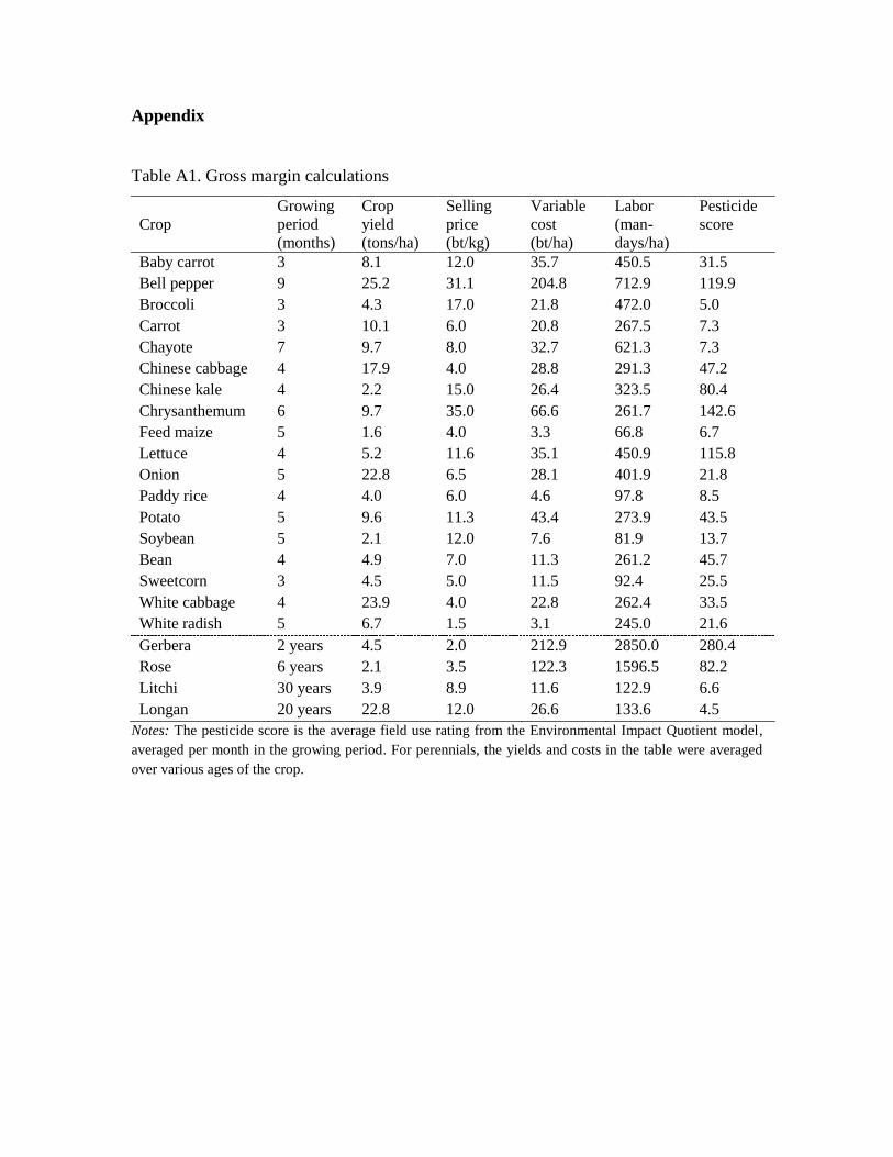
Appendix

Table A1. Gross margin calculations

Crop Growing

period

(months)

Crop

yield

(tons/ha)

Selling

price (bt/kg)

Variable

cost

(bt/ha)

Labor

(man-

days/ha)

Pesticide

score

Baby carrot 3 8.1 12.0 35.7 450.5 31.5

Bell pepper 9 25.2 31.1 204.8 712.9 119.9

Broccoli 3 4.3 17.0 21.8 472.0 5.0

Carrot 3 10.1 6.0 20.8 267.5 7.3

Chayote 7 9.7 8.0 32.7 621.3 7.3

Chinese cabbage 4 17.9 4.0 28.8 291.3 47.2

Chinese kale 4 2.2 15.0 26.4 323.5 80.4

Chrysanthemum 6 9.7 35.0 66.6 261.7 142.6

Feed maize 5 1.6 4.0 3.3 66.8 6.7

Lettuce 4 5.2 11.6 35.1 450.9 115.8

Onion 5 22.8 6.5 28.1 401.9 21.8

Paddy rice 4 4.0 6.0 4.6 97.8 8.5

Potato 5 9.6 11.3 43.4 273.9 43.5

Soybean 5 2.1 12.0 7.6 81.9 13.7

Bean 4 4.9 7.0 11.3 261.2 45.7

Sweetcorn 3 4.5 5.0 11.5 92.4 25.5

White cabbage 4 23.9 4.0 22.8 262.4 33.5

White radish 5 6.7 1.5 3.1 245.0 21.6

Gerbera 2 years 4.5 2.0 212.9 2850.0 280.4

Rose 6 years 2.1 3.5 122.3 1596.5 82.2

Litchi 30 years 3.9 8.9 11.6 122.9 6.6

Longan 20 years 22.8 12.0 26.6 133.6 4.5

Notes: The pesticide score is the average field use rating from the Environmental Impact Quotient model,

averaged per month in the growing period. For perennials, the yields and costs in the table were averaged

over various ages of the crop.