THE DIMENSIONAL FACT MODEL:A CONCEPTUAL MODEL FOR DATA WAREHOUSES 1

MATTEO GOLFARELLI, DARIO MAIO and STEFANO RIZZIDEIS - Università di Bologna, Viale Risorgimento 2, 40136 Bologna, Italy

mgolfarelli,dmaio,srizzi@deis.unibo.it

Data warehousing systems enable enterprise managers to acquire and integrate information fromheterogeneous sources and to query very large databases efficiently. Building a data warehouserequires adopting design and implementation techniques completely different from those underlyingoperational information systems. Though most scientific literature on the design of data warehousesconcerns their logical and physical models, an accurate conceptual design is the necessary foundationfor building a DW which is well-documented and fully satisfies requirements. In this paper weformalize a graphical conceptual model for data warehouses, called Dimensional Fact model, andpropose a semi-automated methodology to build it from the pre-existing (conceptual or logical)schemes describing the enterprise relational database. The representation of reality built using ourconceptual model consists of a set of fact schemes whose basic elements are facts, measures,attributes, dimensions and hierarchies; other features which may be represented on fact schemes arethe additivity of fact attributes along dimensions, the optionality of dimension attributes and theexistence of non-dimension attributes. Compatible fact schemes may be overlapped in order to relateand compare data for drill-across queries. Fact schemes should be integrated with information of theconjectured workload, to be used as the input of logical and physical design phases; to this end, wepropose a simple language to denote data warehouse queries in terms of sets of fact instances.

Keywords: Data warehouse, Conceptual models, Multidimensional data model, Entity-Relationshipmodel

1. Introduction

The database community is devoting increasing attention to the research themesconcerning data warehouses; in fact, the development of decision-support systems willprobably be one of the leading issues for the coming years. The enterprises, after havinginvested a lot of time and resources to build huge and complex information systems, askfor support in quickly obtaining summary information which may help managers inplanning and decision-making. Data warehousing systems address this issue by enablingmanagers to acquire and integrate information from different sources and to query verylarge databases efficiently.

The topic of data warehousing encompasses application tools, architectures,information service and communication infrastructures to synthesize information usefulfor decision-making from distributed heterogeneous operational data sources. This

1 This work was partially supported by the INTERDATA project from the Italian Ministry of Universityand Scientific Research and by Olivetti Sanità.

information is brought together into a single repository, called a data warehouse (DW),suitable for direct querying and analysis and as a source for building logical data martsoriented to specific areas of the enterprise.17

While it is universally recognized that a DW leans on a multidimensional model, littleis said about how to carry out its conceptual design starting from the user requirements.On the other hand, we argue that an accurate conceptual design is the necessary foundationfor building an information system which is both well-documented and fully satisfiesrequirements. The Entity/Relationship (E/R) model is widespread in the enterprises as aconceptual formalism to provide standard documentation for relational informationsystems, and a great deal of effort has been made to use E/R schemes as the input fordesigning non-relational databases as well8; unfortunately, as argued in Ref. 17:

"Entity relation data models [...] cannot be understood by users and they cannot benavigated usefully by DBMS software. Entity relation models cannot be used as the basisfor enterprise data warehouses."

In this paper we present a graphical conceptual model for DWs, called DimensionalFact Model (DFM). The representation of reality built using the DFM is calleddimensional scheme, and consists of a set of fact schemes whose basic elements are facts,dimensions and hierarchies. Compatible fact schemes may be overlapped in order to relateand compare data. Fact schemes may be integrated with information of the conjecturedworkload, expressed in terms of fact instance expressions denoting queries, to be used asthe input of a design phase whose output are the logical and physical schemes of the DW.To this end, we propose a simple language to denote data warehouse queries in terms ofsets of fact instances.

Most information systems implemented in enterprises during the last decade arerelational, and in most cases their analysis documentation consists of E/R schemes. Inthis paper we propose a semi-automated methodology to carry out conceptual modellingstarting from the pre-existing E/R schemes describing the operational information system.In some cases, the E/R documentation held by the enterprise is incomplete or incorrect;often, the only documentation available consists of logical relational schemes. Thus, weshow how our methodology can be applied starting from the database logical scheme.

After surveying the literature on DWs in Section 2, in Section 3 we describe the DFMand introduce fact instance expressions as a formalism to denote DW queries. In Section 4,the overlapping of related fact schemes is discussed. Section 5 describes a methodology forderiving fact schemes from the schemes describing the operational database.

2. Background and literature on data warehousing

From a functional point of view, the data warehouse process consists of three phases:extracting data from distributed operational sources; organizing and integrating dataconsistently into the DW; accessing the integrated data in an efficient and flexible fashion.The first phase encompasses typical issues concerning distributed heterogeneous

information services, such as inconsistent data, incompatible data structures, datagranularity, etc. (for instance, see Ref. 23). The third phase requires capabilities ofaggregate navigation12, optimization of complex queries6, advanced indexing techniques18

and friendly visual interface to be used for On-Line Analytical Processing (OLAP) 7,5 anddata mining.9

As to the second phase, designing the DW requires techniques completely differentfrom those adopted for operational information systems. While most scientific literatureon the design of DWs focuses on specific issues such as materialization of views2,15 andindex selection13,16, no significant effort has been made so far to develop a complete andconsistent design methodology. The apparent lack of interest in the issues related toconceptual design can be explained as follows: (a) data warehousing was initially devisedwithin the industrial world, as a result of practical demands of users who typically do notgive predominant importance to conceptual issues; (b) logical and physical design have aprimary role in optimizing the system performances, which is the main goal in datawarehousing applications.

In Ref. 19, the author proposes an approach to the design of DWs based on a businessmodel of the enterprise which is actually a relational database scheme. Regretfully,conceptual and logical design are mixed up; since logical design is necessarily targetedtowards a logical model (relational in this case), no unifying conceptual model of data isdevised. Ref. 1 and Ref. 14 propose two data models for multidimensional databases andthe related algebras. Both models are at the logical level, thus, they do not addressconceptual modelling issues such as the structure of attribute hierarchies and non-additivity constraints. The approach to conceptual DW modeling presented in Ref. 4shares several ideas with our early work on the topic10, though it is mainly addressedtowards representing attribute hierarchies and neglects other conceptual issues such asadditivity and scheme overlapping.

The multidimensional model may be mapped on the logical level differently dependingon the underlying DBMS. If a DBMS directly supporting the multidimensional model isused, fact attributes are typically represented as the cells of multidimensional arrays whoseindices are determined by key attributes.15 On the other hand, in relational DBMSs themultidimensional model of the DW is mapped in most cases through star schemes17

consisting of a set of dimension tables and a central fact table. Dimension tables arestrongly denormalized and are used to select the facts of interest based on the user queries.The fact table stores fact attributes; its key is defined by importing the keys of thedimension tables.

Different versions of these base schemes have been proposed in order to improve theoverall performances3, handle the sparsity of data20 and optimize the access to aggregateddata.16 In particular, the efficiency issues raised by data warehousing have been dealt withby means of new indexing techniques (see Ref. 22 for a survey), among which wemention bitmap indices.20

3. The Dimensional Fact Model

Definition 1. Let g=(V,E) be a directed, acyclic and weakly connected graph. Wesay g is a quasi-tree with root in v0∈ V if each other vertex vj∈ V can be reached fromv0 through at least one directed path. We will denote with path0j(g)⊆ g a directed pathstarting in v0 and ending in vj; given vi∈ path0j(g), we will denote with pathij (g)⊆ g adirected path starting in vi and ending in vj. We will denote with sub(g,vi)⊂ g thequasi-tree rooted in vi≠v0.

Within a quasi-tree, two or more directed path may converge on the same vertex. A quasi-tree in which the root is connected to each other vertex through exactly one pathdegenerates into a directed tree.

A dimensional scheme consists of a set of fact schemes. The components of factschemes are facts, measures, dimensions and hierarchies. In the following an intuitivedescription of these concepts is given; a formal definition of fact schemes can be found inDefinition 2.

A fact is a focus of interest for the decision-making process; typically, it models anevent occurring in the enterprise world (e.g., sales and shipments). Measures arecontinuously valued (typically numerical) attributes which describe the fact from differentpoints of view; for instance, each sale is measured by its revenue. Dimensions are discreteattributes which determine the minimum granularity adopted to represent facts; typicaldimensions for the sale fact are product, store and date. Hierarchies are made up of discretedimension attributes linked by -to-one relationships, and determine how facts may beaggregated and selected significantly for the decision-making process. The dimension inwhich a hierarchy is rooted defines its finest aggregation granularity; the other dimensionattributes define progressively coarser granularities. A hierarchy on the product dimensionwill probably include the dimension attributes product type, category, department,department manager. Hierarchies may also include non-dimension attributes. A non-dimension attribute contains additional information about a dimension attribute of thehierarchy, and is connected by a -to-one relationship (e.g., the department address); unlikedimension attributes, it cannot be used for aggregation.

Some multidimensional models in the literature focus on treating dimensions andmeasures symmetrically.1,14 This promises to be an important achievement from both thepoint of view of the uniformity of the logical model and that of the flexibility of OLAPoperators. Nevertheless we claim that, at a conceptual level, distinguishing betweenmeasures and dimensions is important since it allows the logical design to be morespecifically aimed at the efficiency required by data warehousing applications.

Definition 2. A fact scheme is a sextuple

f = (M, A, N, R, O, S)

where:

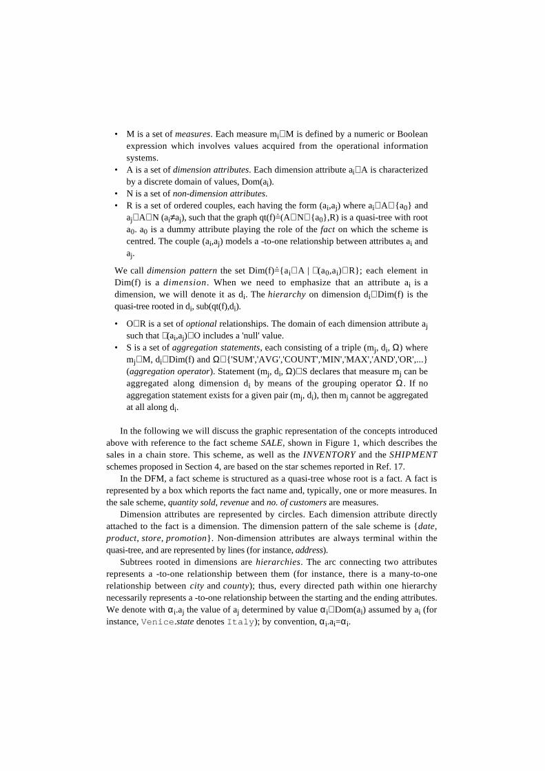
• M is a set of measures. Each measure mi∈ M is defined by a numeric or Booleanexpression which involves values acquired from the operational informationsystems.

• A is a set of dimension attributes. Each dimension attribute ai∈ A is characterizedby a discrete domain of values, Dom(ai).

• N is a set of non-dimension attributes.• R is a set of ordered couples, each having the form (ai,aj) where ai∈ A∪ a0 and

aj∈ A∪ N (ai≠aj), such that the graph qt(f)=.(A∪ N∪ a0,R) is a quasi-tree with root

a0. a0 is a dummy attribute playing the role of the fact on which the scheme iscentred. The couple (ai,aj) models a -to-one relationship between attributes ai andaj.

We call dimension pattern the set Dim(f)=.ai∈ A | ∃ (a0,ai)∈ R; each element in

Dim(f) is a dimension. When we need to emphasize that an attribute ai is adimension, we will denote it as di. The hierarchy on dimension di∈ Dim(f) is thequasi-tree rooted in di, sub(qt(f),di).

• O⊂ R is a set of optional relationships. The domain of each dimension attribute ajsuch that ∃ (ai,aj)∈ O includes a 'null' value.

• S is a set of aggregation statements, each consisting of a triple (mj, di, Ω) wheremj∈ M, di∈ Dim(f) and Ω∈ 'SUM','AVG','COUNT','MIN','MAX','AND','OR',...(aggregation operator). Statement (mj, di, Ω)∈ S declares that measure mj can beaggregated along dimension di by means of the grouping operator Ω. If noaggregation statement exists for a given pair (mj, di), then mj cannot be aggregatedat all along di.

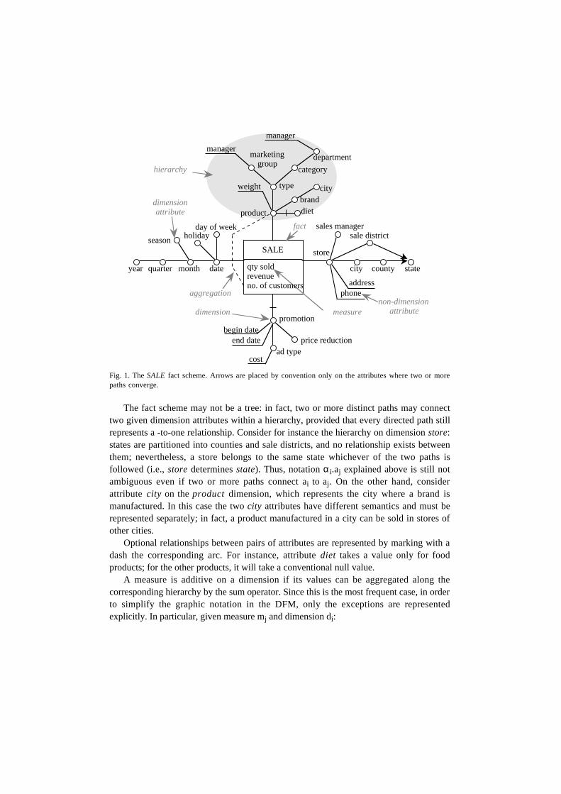
In the following we will discuss the graphic representation of the concepts introducedabove with reference to the fact scheme SALE, shown in Figure 1, which describes thesales in a chain store. This scheme, as well as the INVENTORY and the SHIPMENTschemes proposed in Section 4, are based on the star schemes reported in Ref. 17.

In the DFM, a fact scheme is structured as a quasi-tree whose root is a fact. A fact isrepresented by a box which reports the fact name and, typically, one or more measures. Inthe sale scheme, quantity sold, revenue and no. of customers are measures.

Dimension attributes are represented by circles. Each dimension attribute directlyattached to the fact is a dimension. The dimension pattern of the sale scheme is date,product, store, promotion. Non-dimension attributes are always terminal within thequasi-tree, and are represented by lines (for instance, address).

Subtrees rooted in dimensions are hierarchies. The arc connecting two attributesrepresents a -to-one relationship between them (for instance, there is a many-to-onerelationship between city and county); thus, every directed path within one hierarchynecessarily represents a -to-one relationship between the starting and the ending attributes.We denote with α i.aj the value of aj determined by value α i∈ Dom(ai) assumed by ai (forinstance, Venice .state denotes Italy ); by convention, αi.ai=αi.

state

SALE

product

category

type

quarter month

store

city county

sales manager

address

fact

dimension

hierarchy

non-dimensionattributemeasure

dimensionattribute

year

phone

sale district

date

holidayday of week

season

managermarketing

groupdepartment

weight

branddiet

manager

promotion

price reduction

cost

end datebegin date

ad type

aggregation

qty soldrevenueno. of customers

city

Fig. 1. The SALE fact scheme. Arrows are placed by convention only on the attributes where two or morepaths converge.

The fact scheme may not be a tree: in fact, two or more distinct paths may connecttwo given dimension attributes within a hierarchy, provided that every directed path stillrepresents a -to-one relationship. Consider for instance the hierarchy on dimension store:states are partitioned into counties and sale districts, and no relationship exists betweenthem; nevertheless, a store belongs to the same state whichever of the two paths isfollowed (i.e., store determines state). Thus, notation α i.aj explained above is still notambiguous even if two or more paths connect ai to aj. On the other hand, considerattribute city on the product dimension, which represents the city where a brand ismanufactured. In this case the two city attributes have different semantics and must berepresented separately; in fact, a product manufactured in a city can be sold in stores ofother cities.

Optional relationships between pairs of attributes are represented by marking with adash the corresponding arc. For instance, attribute diet takes a value only for foodproducts; for the other products, it will take a conventional null value.

A measure is additive on a dimension if its values can be aggregated along thecorresponding hierarchy by the sum operator. Since this is the most frequent case, in orderto simplify the graphic notation in the DFM, only the exceptions are representedexplicitly. In particular, given measure mj and dimension di:

1. If (mj, di, 'SUM')∉ S (mj is not additive along di), mj and di are connected by a dashedline labelled with all aggregation operators Ω (if any) such that (mj, di, Ω)∈ S (forinstance, see Figures 1 and 5).

2. If (mj, di, 'SUM')∈ S (mj is additive along di):2.1 If ∃/ Ω≠'SUM' | (mj, di, Ω)∈ S (only sum can be used for aggregation), mj and di

are not graphically connected.2.2 Otherwise (other operators can be used besides the sum), mj and di are connected

by a dashed line labelled with the symbol '+' followed by all the other operatorsΩ≠'SUM' such that (mj, di, Ω)∈ S.

Additivity will be discussed in more detail in Subsection 3.3.

3.1. Fact instances

Given a fact scheme f, each n-tuple of values taken from the domains of the n dimensionsof f defines an elemental cell where one unit of information for the DW can berepresented. We call primary fact instances the units of information present within theDW, each characterized by exactly one value for each measure. We will denote withpf(α 1,...α n) the primary fact instance corresponding to the combination of values(α1,...αn)∈ Dom(d1)×...×Dom(dn). In the sale scheme, each primary instance describes thesales of one product during one day in one store adopting one promotion ('no promotion'should be considered as a particular case of promotion).

Not every possible combination of values necessarily originates a primary factinstance. For instance, in the sale scheme, a missing primary fact instance denotes that aproduct was not on sale on a given day in a given store (null assumption); this is differentfrom having a primary fact instance with qty=0, which denotes that the product remainedunsold. Alternatively, it might be reasonable to assume that all products are always onsale, hence, that a missing primary fact instance denotes that the product remained unsold(zero assumption). Some issues related to these two different interpretations will bediscussed in Subsection 3.3.

Since analysing data at the maximum level of detail is often overwhelming, it may beuseful to aggregate primary fact instances at different levels of abstraction, eachcorresponding to an aggregation pattern; if a given dimension is not interesting for thecurrent analysis, aggregation is carried out over all the possible values that dimension canassume. In the OLAP terminology, this operation is called roll-up.

Definition 3. Given a fact scheme f with n dimensions, a v-dimensionalaggregation pattern (0≤v) is a set P=a1,...av where:

1. ∀ i=1,...v (ai∈ A);2. P≠Dim(f);3. ∀ ai∈ P (∃/ aj∈ P, ai≠aj | aj∈ sub(qt(f),ai)) (i.e., no directed path exists between each

pair of attributes in P).

A dimension di∈ Dim(f) is said to be hidden within P if no attribute of its hierarchysub(qt(f),di) appears within P. An aggregation pattern P is legal with reference tomeasure mj∈ M if

∀ dk | ∃/ (mj, dk, Ω)∈ S dk∈ P

Examples of aggregation patterns in the sale scheme are product,county,month,promotion, state,date (product and promotion are hidden), year,season (two attributesare taken from dimension date), (all dimensions are hidden). Pattern brand,month isillegal with reference to no. of customers since the latter cannot be aggregated along theproduct hierarchy.

Let P=a1,...av be an aggregation pattern, and dh* denote the dimension whosehierarchy includes ah∈ P. The secondary fact instance sf(β1,...βv) corresponding to thecombination of values (β1,...βv)∈ Dom(a1)×...×Dom(av) aggregates the set of primary factinstances

pf(α1,...αn) | ∀ k∈ 1,...n αk∈ Dom(dk) ∧ ∀ h∈ 1,...v αh*.ah=βh

and is characterized by exactly one value for each measure for which P is legal, calculatedby applying an aggregation operator to the values that measure assumes within theprimary fact instances aggregated (see Subsection 3.3).

Figure 2.a shows a primary fact instance on the sale scheme. Figure 2.b shows theprimary fact instances corresponding to the secondary fact instance describing the sales ofproducts of a given category during one day in a city; measure no. of customers is notreported since it cannot be aggregated along the product dimension.

date product

store

qty sold = ...revenue = ...no. of customers = ...

(a)

dateproduct

store

qty sold = Σ...revenue = Σ...

category

city

(b)

Fig. 2. A primary (a) and a secondary (b) fact istance for the SALE scheme (dimension promotion is omittedfor clarity).

In the following, we will use sometimes the term pattern to denote either thedimension pattern or an aggregation pattern.

3.2. Representing queries on the dimensional scheme

In general, querying an information system means linking different concepts through user-defined paths in order to retrieve some data of interest; in particular, for relationaldatabases this is done by formulating a set of joins to connect relation schemes. On theother hand, a substantial amount of queries on DWs are aimed at extracting summary datato fill structured reports to be analysed for decisional or statistical purposes. Thus, withinour framework, a typical DW query can be represented by the set of fact instances, at anyaggregation level, whose measure values are to be retrieved.

In this subsection we discuss how sets of fact instances can be denoted by writing factinstance expressions. The simple language we propose is aimed at defining, with referenceto a dimensional scheme, the queries forming the expected workload for the DW, to beused for logical design; thus, it focuses on which data must be retrieved and at which levelthey must be consolidated.

A fact instance expression has the general form:

<fact instance expression> ::= <fact name> ( <pattern clause> ; <selection clause> )<pattern clause> ::= comma-list of <pattern elements><pattern elements> ::= <dimension name> | <dimension name>.<attribute name><selection clause> ::= comma-list of <predicate>

The pattern clause describes a pattern. The selection clause contains a set of Booleanpredicates which may either select a subset of the aggregated fact instances or affect theway fact instances are aggregated. If an attribute involved either in a pattern clause or in aselection clause is not a dimension, it should be referenced by prefixing its dimensionname.

The value(s) assumed by a measure within the fact instance(s) described by a factinstance expression is(are) denoted as follows:

<measure values> ::= <fact instance expression>.<measure>

Given a fact scheme f having n dimensions d1,...dn, consider the fact instanceexpression

f(d1,...dp,ap+1,...av ; e1(bi1),...eh(bih)) (1)

where we have assumed, without loss of generality, that:

• The first p pattern elements involve a dimension and the other v−p involve adimension attribute (0≤p≤v).

• Each Boolean predicate ej (j=1,...h, h≥0) involves one attribute bij belonging to thehierarchy rooted in dij* , which may also be hidden.

If p=v=n (i.e., the pattern clause describes the dimension pattern), expression (1)denotes the set of primary fact instances

pf(α1,...αn) | ∀ k∈ 1,...n αk∈ Dom(dk) ∧ ∀ j∈ 1,...h ej(α i j* .bij)

For instance, the expression

SALE(date, product, store, promotion ; date.year>='1995',product='P5').qtySold

denotes the quantities of product P5 sold in each store, with each promotion, during eachday since 1995.

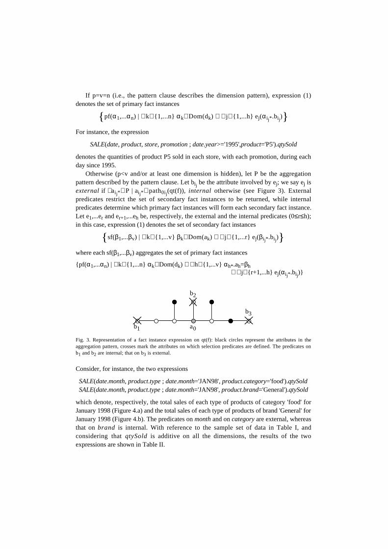
Otherwise (p<v and/or at least one dimension is hidden), let P be the aggregationpattern described by the pattern clause. Let bij be the attribute involved by ej; we say ej isexternal if ∃ aij* ∈ P | aij* ∈ path0ij(qt(f)), internal otherwise (see Figure 3). Externalpredicates restrict the set of secondary fact instances to be returned, while internalpredicates determine which primary fact instances will form each secondary fact instance.Let e1,...er and er+1,...eh be, respectively, the external and the internal predicates (0≤r≤h);in this case, expression (1) denotes the set of secondary fact instances

sf(β1,...βv) | ∀ k∈ 1,...v βk∈ Dom(ak) ∧ ∀ j∈ 1,...r ej(βi j* .bij)

where each sf(β1,...βv) aggregates the set of primary fact instances

pf( α1,...αn) | ∀ k∈ 1,...n αk∈ Dom(dk) ∧ ∀ h∈ 1,...v αh*.ah=βh∧ ∀ j∈ r+1,...h ej(αij* .bij)

a0b1

b2

b3

Fig. 3. Representation of a fact instance expression on qt(f): black circles represent the attributes in theaggregation pattern, crosses mark the attributes on which selection predicates are defined. The predicates onb1 and b2 are internal; that on b3 is external.

Consider, for instance, the two expressions

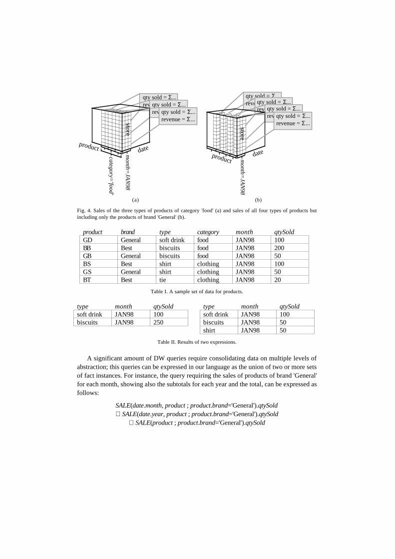
SALE(date.month, product.type ; date.month='JAN98', product.category='food').qtySoldSALE(date.month, product.type ; date.month='JAN98', product.brand='General').qtySold

which denote, respectively, the total sales of each type of products of category 'food' forJanuary 1998 (Figure 4.a) and the total sales of each type of products of brand 'General' forJanuary 1998 (Figure 4.b). The predicates on month and on category are external, whereasthat on brand is internal. With reference to the sample set of data in Table I, andconsidering that qtySold is additive on all the dimensions, the results of the twoexpressions are shown in Table II.

qty sold = Σ...revenue = Σ...

product date

store

qty sold = Σ...revenue = Σ...

mo

nth

=JA

N9

8

cate

go

ry='fo

od

'

qty sold = Σ...revenue = Σ...

qty sold = Σ...revenue = Σ...qty sold = Σ...

revenue = Σ...

productdate

store

qty sold = Σ...revenue = Σ...

mo

nth

=JA

N9

8

qty sold = Σ...revenue = Σ...

(a) (b)

Fig. 4. Sales of the three types of products of category 'food' (a) and sales of all four types of products butincluding only the products of brand 'General' (b).

product brand type category month qtySoldGD General soft drink food JAN98 100BB Best biscuits food JAN98 200GB General biscuits food JAN98 50BS Best shirt clothing JAN98 100GS General shirt clothing JAN98 50BT Best tie clothing JAN98 20

Table I. A sample set of data for products.

type month qtySold type month qtySoldsoft drink JAN98 100 soft drink JAN98 100biscuits JAN98 250 biscuits JAN98 50

shirt JAN98 50

Table II. Results of two expressions.

A significant amount of DW queries require consolidating data on multiple levels ofabstraction; this queries can be expressed in our language as the union of two or more setsof fact instances. For instance, the query requiring the sales of products of brand 'General'for each month, showing also the subtotals for each year and the total, can be expressed asfollows:

SALE(date.month, product ; product.brand='General').qtySold∪ SALE(date.year, product ; product.brand='General').qtySold

∪ SALE(product ; product.brand='General').qtySold

3.3. Add i t i v i t y

Aggregation requires defining a proper operator to compose the measure valuescharacterizing primary fact instances into measure values characterizing each secondary factinstance.

Definition 4. Given a fact scheme f, measure mj∈ M is said to be aggregable ondimension dk∈ Dim(f) if ∃ (mj, dk, Ω)∈ S, non-aggregable otherwise. Measure mj issaid to be additive on dk if ∃ (mj, dk, 'SUM')∈ S, non-additive otherwise.

As a guideline, most measures in a fact scheme should be additive. An example ofadditive measure in the sale scheme is qty sold: the quantity sold for a given sales manageris the sum of the quantities sold for all the stores managed by that sales manager.

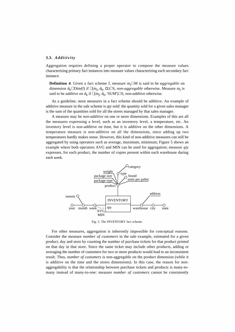
A measure may be non-additive on one or more dimensions. Examples of this are allthe measures expressing a level, such as an inventory level, a temperature, etc. Aninventory level is non-additive on time, but it is additive on the other dimensions. Atemperature measure is non-additive on all the dimensions, since adding up twotemperatures hardly makes sense. However, this kind of non-additive measures can still beaggregated by using operators such as average, maximum, minimum; Figure 5 shows anexample where both operators AVG and MIN can be used for aggregation; measure qtyexpresses, for each product, the number of copies present within each warehouse duringeach week.

state

INVENTORY

product

qty

category

type

month warehouse city

address

year week

season

weightpackage size brand

AVG, MIN

units per palletpackage type

Fig. 5. The INVENTORY fact scheme.

For other measures, aggregation is inherently impossible for conceptual reasons.Consider the measure number of customers in the sale example, estimated for a givenproduct, day and store by counting the number of purchase tickets for that product printedon that day in that store. Since the same ticket may include other products, adding oraveraging the number of customers for two or more products would lead to an inconsistentresult. Thus, number of customers is non-aggregable on the product dimension (while itis additive on the time and the stores dimensions). In this case, the reason for non-aggregability is that the relationship between purchase tickets and products is many-to-many instead of many-to-one: measure number of customers cannot be consistently

aggregated on the product dimension, whatever operator is used, unless the grain of factinstances is made finer. If mj is non-aggregable on dk, any aggregation pattern notincluding dk is illegal with reference to mj.

Given a measure mj aggregable on dk by operator Ω and the aggregation patternP=d1,...,dk-1,ak,dk+1,...dn, which includes all the dimensions except dk which isrepresented by any other dimension attribute ak belonging to its hierarchy, the value of mjmay be computed for each secondary fact instance at pattern P as:

f(d1,...ak,...dn ; d1=α1,...ak=αk,...dn=αn).mj =

= Ωβ∈ Dom(dk)|β.ak=αk

f(d1,...dk,...dn ; d1=α1,...dk=β,...dn=αn).mj

for each αk∈ Dom(ak), α i∈ Dom(di) (i=1,...n; i≠k). Similarly, if dk is hidden within P, itis:

f(d1,...dk-1,dk+1,...dn ; d1=α1,...dn=αn).mj =

= Ωβ∈ Dom(dk)

f(d1,...dk,...dn ; d1=α1,...dk=β,...dn=αn).mj

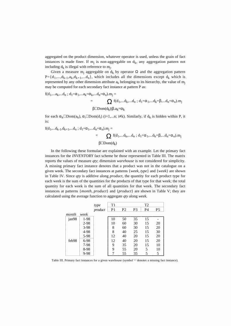
In the following these formulae are explained with an example. Let the primary factinstances for the INVENTORY fact scheme be those represented in Table III. The matrixreports the values of measure qty; dimension warehouse is not considered for simplicity.A missing primary fact instance denotes that a product was not in the catalogue on agiven week. The secondary fact instances at patterns week, type and week are shownin Table IV. Since qty is additive along product, the quantity for each product type foreach week is the sum of the quantities for the products of that type for that week; the totalquantity for each week is the sum of all quantities for that week. The secondary factinstances at patterns month, product and product are shown in Table V; they arecalculated using the average function to aggregate qty along week.

type T1 T2product P1 P2 P3 P4 P5

month weekjan98 1-98 10 50 35 15 -

2-98 10 60 30 15 203-98 8 60 30 15 204-98 8 40 25 15 305-98 12 40 20 15 20

feb98 6-98 12 40 20 15 207-98 9 35 20 15 108-98 9 55 20 5 109-98 7 55 35 5 5

Table III. Primary fact instances for a given warehouse (symbol '-' denotes a missing fact instance).

type T1 T2month week

jan98 1-98 95 15 1102-98 100 35 1353-98 98 35 1334-98 73 45 1185-98 72 35 107

feb98 6-98 72 35 1077-98 64 25 898-98 84 15 999-98 97 10 107

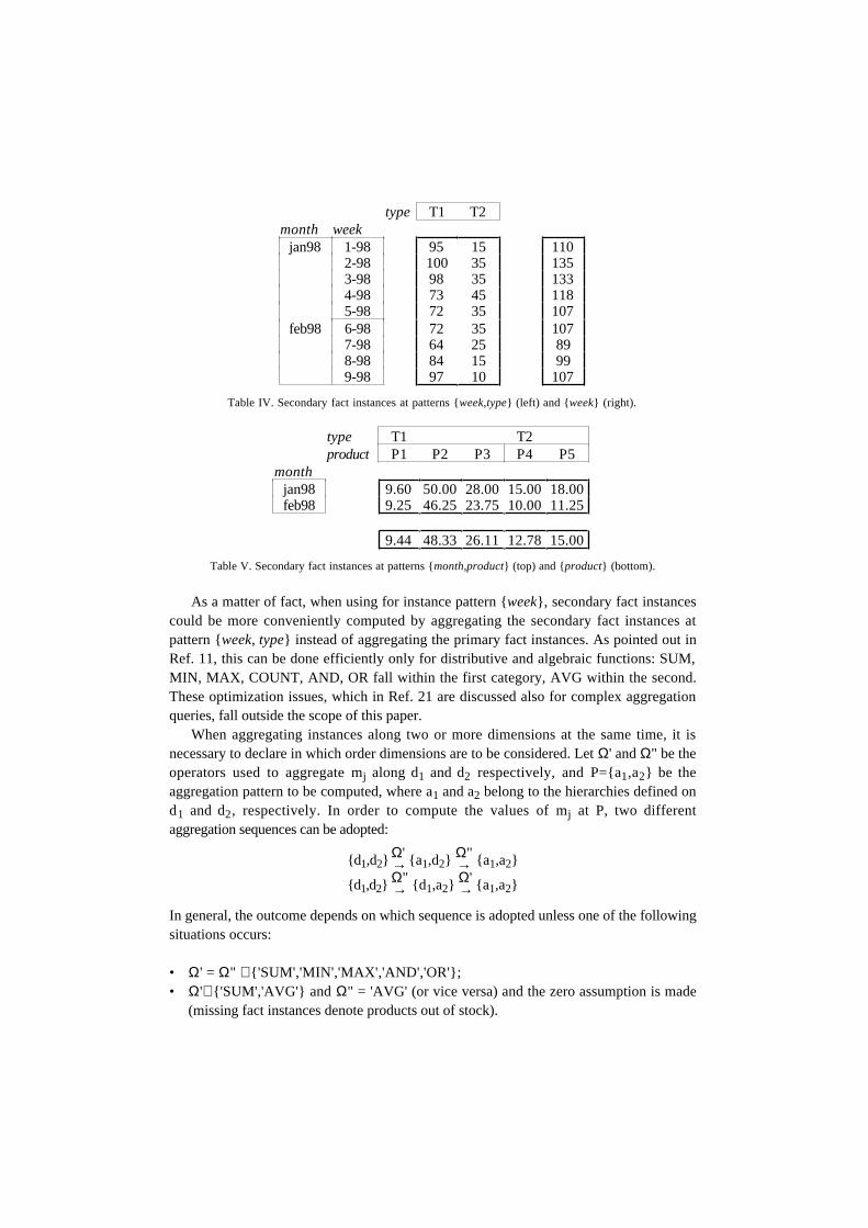
Table IV. Secondary fact instances at patterns week,type (left) and week (right).

type T1 T2product P1 P2 P3 P4 P5

monthjan98 9.60 50.00 28.00 15.00 18.00feb98 9.25 46.25 23.75 10.00 11.25

9.44 48.33 26.11 12.78 15.00

Table V. Secondary fact instances at patterns month,product (top) and product (bottom).

As a matter of fact, when using for instance pattern week, secondary fact instancescould be more conveniently computed by aggregating the secondary fact instances atpattern week, type instead of aggregating the primary fact instances. As pointed out inRef. 11, this can be done efficiently only for distributive and algebraic functions: SUM,MIN, MAX, COUNT, AND, OR fall within the first category, AVG within the second.These optimization issues, which in Ref. 21 are discussed also for complex aggregationqueries, fall outside the scope of this paper.

When aggregating instances along two or more dimensions at the same time, it isnecessary to declare in which order dimensions are to be considered. Let Ω' and Ω" be theoperators used to aggregate mj along d1 and d2 respectively, and P=a1,a2 be theaggregation pattern to be computed, where a1 and a2 belong to the hierarchies defined ond1 and d2, respectively. In order to compute the values of mj at P, two differentaggregation sequences can be adopted:

d1,d2 →Ω' a1,d2 →

Ω" a1,a2

d1,d2 →Ω" d1,a2 →

Ω' a1,a2

In general, the outcome depends on which sequence is adopted unless one of the followingsituations occurs:

• Ω' = Ω" ∈ 'SUM','MIN','MAX','AND','OR';• Ω'∈ 'SUM','AVG' and Ω" = 'AVG' (or vice versa) and the zero assumption is made

(missing fact instances denote products out of stock).

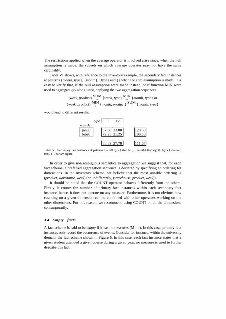
The restrictions applied when the average operator is involved arise since, when the nullassumption is made, the subsets on which average operates may not have the samecardinality.

Table VI shows, with reference to the inventory example, the secondary fact instancesat patterns month, type, month, type and when the zero assumption is made. It iseasy to verify that, if the null assumption were made instead, or if function MIN wereused to aggregate qty along week, applying the two aggregation sequences

week, product →SUM week, type →

MIN month, type or

week, product →MIN month, product →

SUM month, type

would lead to different results.

type T1 T2month

jan98 87.60 33.00 120.60feb98 79.25 21.25 100.50

83.89 27.78 111.67

Table VI. Secondary fact instances at patterns month,type (top left), month (top right), type (bottomleft), (bottom right).

In order to give non ambiguous semantics to aggregation we suggest that, for eachfact scheme, a preferred aggregation sequence is declared by specifying an ordering fordimensions. In the inventory scheme, we believe that the most suitable ordering is(product, warehouse, week) (or, indifferently, (warehouse, product, week)).

It should be noted that the COUNT operator behaves differently from the others.Firstly, it counts the number of primary fact instances within each secondary factinstance, hence, it does not operate on any measure. Furthermore, it is not obvious howcounting on a given dimension can be combined with other operators working on theother dimensions. For this reason, we recommend using COUNT on all the dimensionscontemporarily.

3.4. Empty facts

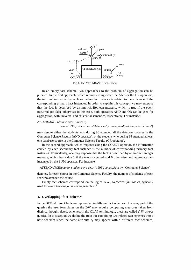
A fact scheme is said to be empty if it has no measures (M=∅ ). In this case, primary factinstances only record the occurrence of events. Consider for instance, within the universitydomain, the fact scheme shown in Figure 6. In this case, each fact instance states that agiven student attended a given course during a given year; no measure is used to furtherdescribe this fact.

ATTENDANCE

studentnationality

age

course

faculty

area

year

address sex

COUNT

name

COUNT

COUNT

Fig. 6. The ATTENDANCE fact scheme.

In an empty fact scheme, two approaches to the problem of aggregation can bepursued. In the first approach, which requires using either the AND or the OR operators,the information carried by each secondary fact instance is related to the existence of thecorresponding primary fact instances. In order to explain this concept, we may supposethat the fact is described by an implicit Boolean measure, which is true if the eventoccurred and false otherwise: in this case, both operators AND and OR can be used foraggregation, with universal and existential semantics, respectively. For instance:

ATTENDANCE(course.area, student ;year='1998', course.area='Databases', course.faculty='Computer Science')

may denote either the students who during 98 attended all the database courses in theComputer Science Faculty (AND operator), or the students who during 98 attended at leastone database course in the Computer Science Faculty (OR operator).

In the second approach, which requires using the COUNT operator, the informationcarried by each secondary fact instance is the number of corresponding primary factinstances. Equivalently, one may suppose that the fact is described by an implicit integermeasure, which has value 1 if the event occurred and 0 otherwise, and aggregate factinstances by the SUM operator. For instance:

ATTENDANCE(course, student.sex ; year='1998', course.faculty='Computer Science')

denotes, for each course in the Computer Science Faculty, the number of students of eachsex who attended the course.

Empty fact schemes correspond, on the logical level, to factless fact tables, typicallyused for event tracking or as coverage tables.17

4. Overlapping fact schemes

In the DFM, different facts are represented in different fact schemes. However, part of thequeries the user formulates on the DW may require comparing measures taken fromdistinct, though related, schemes; in the OLAP terminology, these are called drill-acrossqueries. In this section we define the rules for combining two related fact schemes into anew scheme; since the same attribute ai may appear within different fact schemes,

possibly with different domains, we will denote with Domf(ai) the domain of ai withinscheme f.

Def in i t ion 5 . Two fact schemes f '=(M',A',N',R',O',S') andf"=(M",A",N",R",O",S") are said to be compatible if they share at least onedimension attribute: A'∩A"≠∅ . Attribute ai is considered to be common to f' and f"if, within f' and f", it has the same semantics and if Domf'(ai)∩Domf"(ai)≠∅ .

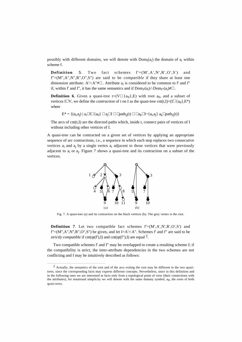
Definition 6. Given a quasi-tree t=(V∪ a0,E) with root a0, and a subset ofvertices I⊆ V, we define the contraction of t on I as the quasi-tree cnt(t,I)=(I∪ a0,E*)where

E* = (ai,aj) | ai∈ I∪ a0 ∧ aj∈ I ∧ ∃ pathij(t) ∧ ∀ ak∈ I−ai,aj ak∉ pathij(t)

The arcs of cnt(t,I) are the directed paths which, inside t, connect pairs of vertices of Iwithout including other vertices of I.

A quasi-tree can be contracted on a given set of vertices by applying an appropriatesequence of arc contractions, i.e., a sequence in which each step replaces two consecutivevertices ai and aj by a single vertex ai adjacent to those vertices that were previouslyadjacent to ai or aj. Figure 7 shows a quasi-tree and its contraction on a subset of thevertices.

1 2 3

4 5 6 7 8

10 119

5 7

3

109(a) (b)

Fig. 7. A quasi-tree (a) and its contraction on the black vertices (b). The grey vertex is the root.

Definition 7. Let two compatible fact schemes f'=(M',A',N',R',O',S') andf"=(M",A",N",R",O",S") be given, and let I=A'∩A". Schemes f' and f" are said to bestrictly compatible if cnt(qt(f'),I) and cnt(qt(f"),I) are equal 2.

Two compatible schemes f' and f" may be overlapped to create a resulting scheme f; ifthe compatibility is strict, the inter-attribute dependencies in the two schemes are notconflicting and f may be intuitively described as follows:

2 Actually, the semantics of the root and of the arcs exiting the root may be different in the two quasi-trees, since the corresponding facts may express different concepts. Nevertheless, since in this definition andin the following ones we are interested in facts only from a topological point of view (their connections withthe attributes), for notational simplicity we will denote with the same dummy symbol, a0, the roots of bothquasi-trees.

stateSHIPMENT

product

qty shipped.....

category

type

quarter monthship to city

address

year

corporate

customer

date

season

department

weightpackage size brand

diet

manager

deal

termsincentive

ship from

address

contact personship mode

addressallowance

typecarrier

order dateinvoice number

(a)

SHIPMENT⊗

INVENTORY

product

qty shippedinventory qty.....

category

type

month

year

season

weightpackage size brand

AVG,MIN

(b)

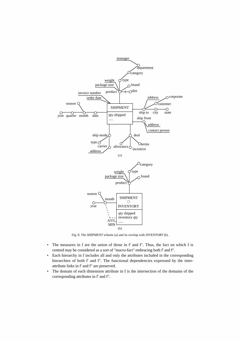
Fig. 8. The SHIPMENT scheme (a) and its overlap with INVENTORY (b).

• The measures in f are the union of those in f' and f". Thus, the fact on which f iscentred may be considered as a sort of "macro-fact" embracing both f' and f".

• Each hierarchy in f includes all and only the attributes included in the correspondinghierarchies of both f' and f". The functional dependencies expressed by the inter-attribute links in f' and f" are preserved.

• The domain of each dimension attribute in f is the intersection of the domains of thecorresponding attributes in f' and f".

• An inter-attribute link in f is optional if at least one of the links in the correspondingpaths in f' or f" is optional.

• Aggregation statements of f' and f" are preserved in f.

Formally:

Definition 8. Given two strictly compatible schemes f' and f", we define theoverlap of f' and f" as the scheme f'⊗ f"=(M,A,N,R,O,S) where:

M = M'∪ M"A = A'∩A"∀ ai∈ A (Domf'⊗ f"(ai) = Domf'(ai)∩Domf"(ai))

N = N'∩N"R = (ai,aj) | (ai,aj)∈ cnt(qt(f'),A) = (ai,aj) | (ai,aj)∈ cnt(qt(f"),A)O = (ai,aj)∈ R | ∃ (aw,az)∈ O' | (aw,az)∈ pathij (qt(f')) ∨ ∃ (aw,az)∈ O" |

(aw,az)∈ pathij(qt(f"))S = (mj,di,Ω) | di∈ Dim(f'⊗ f") ∧ (∃ (mj,dk,Ω)∈ S' ∧ di∈ sub(qt(f'),dk)) ∨

(∃ (mj,dk,Ω)∈ S" ∧ di∈ sub(qt(f"),dk))

Figure 8 shows the overlapping between the two strictly compatible schemesINVENTORY and SHIPMENT, which share the time and the product dimensions. Thescheme resulting from overlapping can be used, for instance, to compare the quantitiesshipped and stored for each product.

As a matter of fact, overlapping may be extended by considering more accurately theinformation expressed by the hierarchies in the two source schemes. Consider for instancethe INVENTORY and SHIPMENT schemes, which include two compatible hierarchies ondimensions week and date, respectively. Based on Definition 8, their overlap shouldinclude only attributes month, year and season. Attribute date cannot definitely beincluded, since in the INVENTORY scheme it is impossible to disaggregate the primaryfact instances at the date level. On the other hand, quarter could be included: in fact, themonths represented in the overlap are those represented in both the source schemes, andfor each month the quarter is known from SHIPMENT.

Even two non-strictly compatible schemes can be overlapped; since in this case thetwo contracted quasi-trees are different, there must be one or more conflicts in the inter-attribute dependencies in the two schemes. The resulting scheme is defined as in the caseof strict compatibility, except that each conflict is solved by representing an inter-attributedependency which subsumes both conflicting dependencies. Consider the example inFigure 9, where two non-strictly compatible fact schemes (a) and (b) are shown. Thedependencies expressed by the two quasi-trees are as follows:

(a) (b)

root → 1,2,3 root → 1,22 → 4 2 → 54 → 5 5 → 4

1 → 3

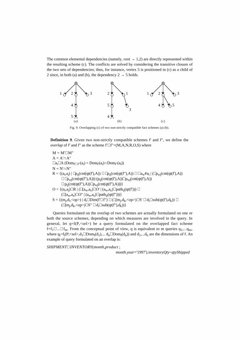
The common elemental dependencies (namely, root → 1,2) are directly represented withinthe resulting scheme (c). The conflicts are solved by considering the transitive closure ofthe two sets of dependencies; thus, for instance, vertex 5 is positioned in (c) as a child of2 since, in both (a) and (b), the dependency 2 → 5 holds.

1 2 3

4

5

2 1

35

4

1 2 3

4 5

(a) (b) (c)

Fig. 9. Overlapping (c) of two non-strictly compatible fact schemes (a) (b).

Definition 9. Given two non-strictly compatible schemes f' and f", we define theoverlap of f' and f" as the scheme f'⊗ f"=(M,A,N,R,O,S) where

M = M'∪ M"A = A'∩A"∀ ai∈ A (Domf'⊗ f"(ai) = Domf'(ai)∩Domf"(ai))

N = N'∩N"R = (ai,aj) | ∃ pij(cnt(qt(f'),A)) ∧ ∃ pij(cnt(qt(f"),A)) ∧ ∀ aw≠ai | (∃ pwj(cnt(qt(f'),A))

∧ ∃ pwj(cnt(qt(f"),A))) (pij(cnt(qt(f'),A))⊂ pwj(cnt(qt(f'),A))∧ pij(cnt(qt(f"),A))⊂ pwj(cnt(qt(f"),A)))

O = (ai,aj)∈ R | (∃ (aw,az)∈ O' | (aw,az)∈ pathij(qt(f'))) ∨(∃ (aw,az)∈ O" | (aw,az)∈ pathij(qt(f")))

S = (mj,di,<op>) | di∈ Dim(f'⊗ f") ∧ (∃ (mj,dk,<op>)∈ S' ∧ di∈ sub(qt(f'),dk)) ∨ (∃ (mj,dk,<op>)∈ S" ∧ di∈ sub(qt(f"),dk))

Queries formulated on the overlap of two schemes are actually formulated on one orboth the source schemes, depending on which measures are involved in the query. Ingeneral, let q=f(P,<sel>) be a query formulated on the overlapped fact schemef=f1⊗ ...⊗ fm. From the conceptual point of view, q is equivalent to m queries q1,...qm,where qi=fi(P;<sel>,d1∈ Domf(d1),... dn∈ Domf(dn)) and d1,...dn are the dimensions of f. Anexample of query formulated on an overlap is:

SHIPMENT⊗ INVENTORY(month,product ;month.year='1997').inventoryQty−qtyShipped

5. Conceptual design from relational schemes

The methodology we outline in this section to build a DF model starting from thedocumentation describing the operational relational database consists of the followingsteps:

1. Defining facts.2. For each fact:

a. Building the attribute tree.b. Pruning and grafting the attribute tree.c. Defining dimensions.d. Defining measures.e. Defining hierarchies.

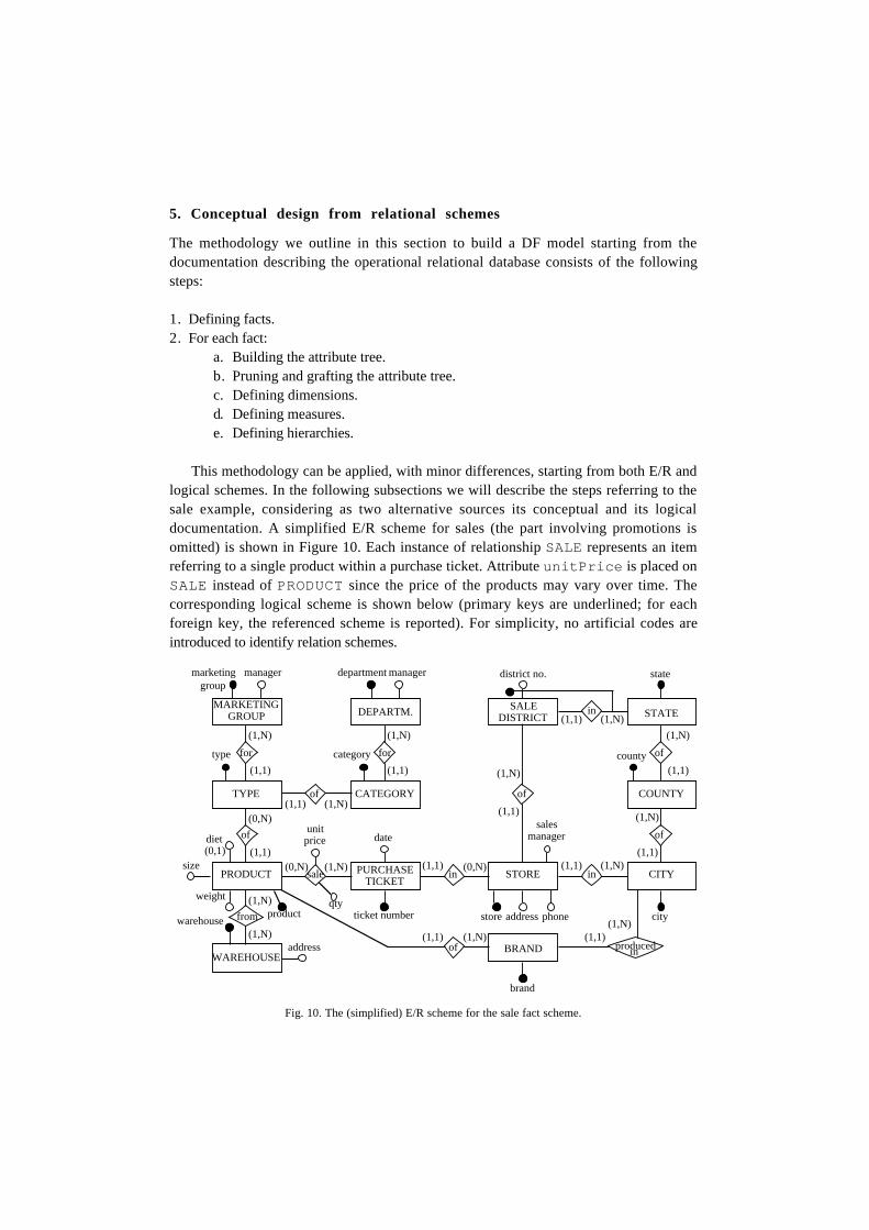
This methodology can be applied, with minor differences, starting from both E/R andlogical schemes. In the following subsections we will describe the steps referring to thesale example, considering as two alternative sources its conceptual and its logicaldocumentation. A simplified E/R scheme for sales (the part involving promotions isomitted) is shown in Figure 10. Each instance of relationship SALE represents an itemreferring to a single product within a purchase ticket. Attribute unitPrice is placed onSALE instead of PRODUCT since the price of the products may vary over time. Thecorresponding logical scheme is shown below (primary keys are underlined; for eachforeign key, the referenced scheme is reported). For simplicity, no artificial codes areintroduced to identify relation schemes.

TYPE

PRODUCT

CATEGORY

STORE CITY

(1,1)(0,N)

(1,1) (1,N)

(1,1) (0,N) (1,1) (1,N)

(0,N)

date

qty

unit price

PURCHASETICKET

(1,N)

type category

product

salesmanager

ticket number store city

of

sale

of

in in

weight

diet(0,1)

address

MARKETING GROUP

(1,1)

(1,N)

marketinggroup

for

manager

DEPARTM.

(1,1)

(1,N)

department

for

manager

phone

COUNTY

(1,1)

(1,N)

county

of

STATE

(1,1)

(1,N)

state

of

BRAND

brand

(1,1)(1,N)

(1,1) (1,N)of

WAREHOUSE

(1,N)

(1,N)

fromwarehouse

SALEDISTRICT

district no.

(1,1) (1,N)in

(1,1)

(1,N)

of

address producedin

size

Fig. 10. The (simplified) E/R scheme for the sale fact scheme.

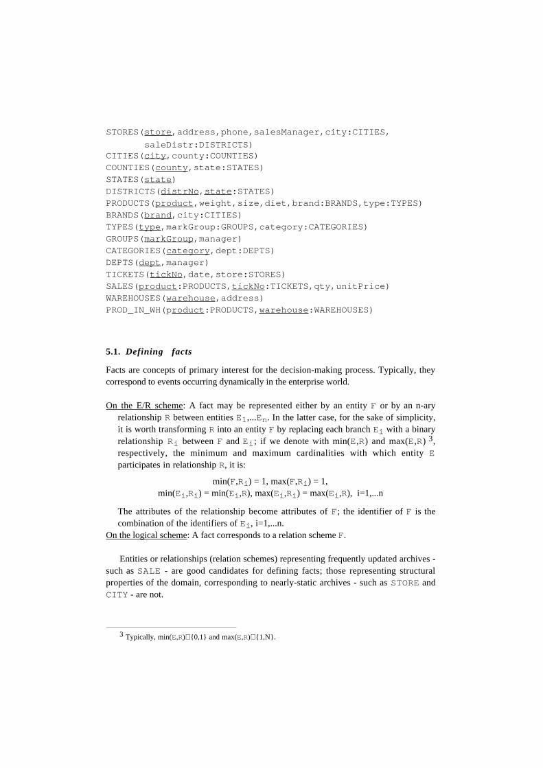
STORES(store,address,phone,salesManager,city:CITIES,

saleDistr:DISTRICTS)CITIES( city,county:COUNTIES)COUNTIES(county,state:STATES)STATES(state)DISTRICTS( distrNo, state:STATES)PRODUCTS(product,weight,size,diet,brand:BRANDS,type:TYPES)BRANDS(brand,city:CITIES)TYPES(type,markGroup:GROUPS,category:CATEGORIES)GROUPS(markGroup,manager)CATEGORIES(category,dept:DEPTS)DEPTS(dept,manager)TICKETS( tickNo,date,store:STORES)SALES(product:PRODUCTS, tickNo:TICKETS,qty,unitPrice)WAREHOUSES(warehouse,address)PROD_IN_WH(product:PRODUCTS, warehouse:WAREHOUSES)

5.1. Defining facts

Facts are concepts of primary interest for the decision-making process. Typically, theycorrespond to events occurring dynamically in the enterprise world.

On the E/R scheme: A fact may be represented either by an entity F or by an n-aryrelationship R between entities E1,...En. In the latter case, for the sake of simplicity,it is worth transforming R into an entity F by replacing each branch Ei with a binaryrelationship Ri between F and Ei ; if we denote with min(E,R) and max(E,R) 3,respectively, the minimum and maximum cardinalities with which entity Eparticipates in relationship R, it is:

min(F,Ri ) = 1, max(F,Ri ) = 1,min(Ei ,Ri ) = min(Ei ,R), max(Ei ,Ri ) = max(Ei ,R), i=1,...n

The attributes of the relationship become attributes of F; the identifier of F is thecombination of the identifiers of Ei , i=1,...n.

On the logical scheme: A fact corresponds to a relation scheme F.

Entities or relationships (relation schemes) representing frequently updated archives -such as SALE - are good candidates for defining facts; those representing structuralproperties of the domain, corresponding to nearly-static archives - such as STORE andCITY - are not.

3 Typically, min(E,R)∈ 0,1 and max(E,R)∈ 1,N.

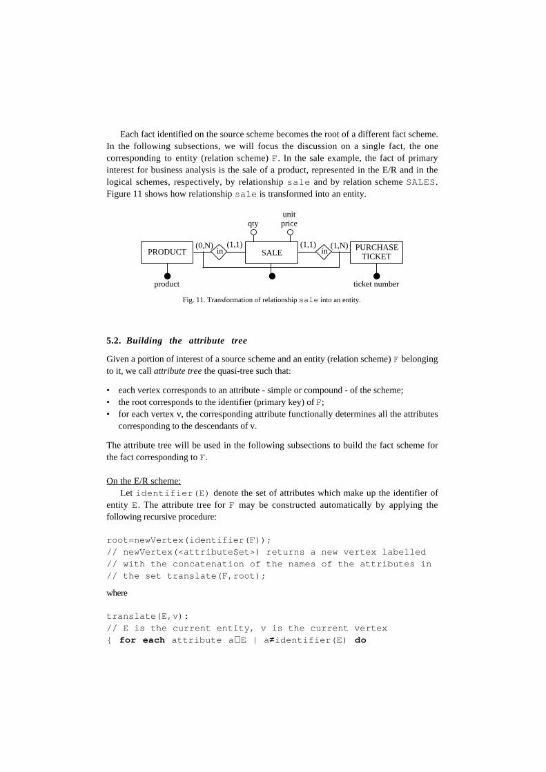
Each fact identified on the source scheme becomes the root of a different fact scheme.In the following subsections, we will focus the discussion on a single fact, the onecorresponding to entity (relation scheme) F. In the sale example, the fact of primaryinterest for business analysis is the sale of a product, represented in the E/R and in thelogical schemes, respectively, by relationship sale and by relation scheme SALES.Figure 11 shows how relationship sale is transformed into an entity.

PRODUCT(1,1)(0,N)

qty

product

in

unit price

PURCHASETICKET

(1,N)

ticket number

in(1,1)

SALE

Fig. 11. Transformation of relationship sale into an entity.

5.2. Building the attribute tree

Given a portion of interest of a source scheme and an entity (relation scheme) F belongingto it, we call attribute tree the quasi-tree such that:

• each vertex corresponds to an attribute - simple or compound - of the scheme;• the root corresponds to the identifier (primary key) of F;• for each vertex v, the corresponding attribute functionally determines all the attributes

corresponding to the descendants of v.

The attribute tree will be used in the following subsections to build the fact scheme forthe fact corresponding to F.

On the E/R scheme:Let identifier(E) denote the set of attributes which make up the identifier of

entity E. The attribute tree for F may be constructed automatically by applying thefollowing recursive procedure:

root=newVertex(identifier(F));// newVertex(<attributeSet>) returns a new vertex labelled// with the concatenation of the names of the attributes in// the set translate(F,root);

where

translate(E,v):// E is the current entity, v is the current vertex for each attribute a ∈ E | a ≠identifier(E) do

addChild(v,newVertex(a)); // adds child a to vertex vfor each entity G connected to E

by a relationship R | max(E,R)=1 do for each attribute b ∈ R do

addChild(v,newVertex(b));next=newVertex(identifier(G));addChild(v,next);translate(G,next);

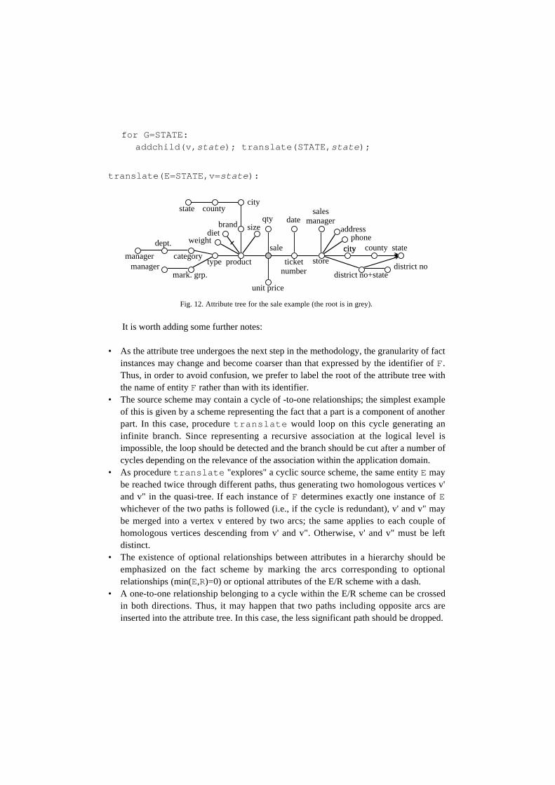
In the following we illustrate how procedure translate works by showing in astep-by-step fashion how a branch of the attribute tree for the sale example is generated;the resulting attribute tree is shown in Figure 12.

root=newVertex( ticketNumber+product ) // renamed sale

translate(E=SALE,v= sale ):addchild(v, qty ); addchild(v, unitPrice );for G=PURCHASE TICKET:

addchild(v, ticketNumber );translate(PURCHASE TICKET, ticketNumber );

for G=PRODUCT:addchild(v, product ); translate(PRODUCT, product );

translate(E=PURCHASE TICKET,v= ticketNumber ):addchild(v, date );for G=STORE:

addchild(v, store ); translate(STORE, store );

translate(E=STORE,v= store ):addchild(v, address ); addchild(v, phone );addchild(v, salesManager );for G=SALE DISTRICT:

addchild(v, districtNo+state );translate(SALE DISTRICT, districtNo+state );

for G=CITY:addchild(v, city ); translate(CITY, city );

translate(E=SALE DISTRICT,v= districtNo+state ):addchild(v, districtNo );

for G=STATE:addchild(v, state ); translate(STATE, state );

translate(E=STATE,v= state ):

district no

unit price

qty

ticketnumber

date

store

salesmanager

city state

product

brand

typecategory

addressdiet

city

weightdept.

manager

mark. grp.manager

phone

county

district no+state

size

city

state

countysale

Fig. 12. Attribute tree for the sale example (the root is in grey).

It is worth adding some further notes:

• As the attribute tree undergoes the next step in the methodology, the granularity of factinstances may change and become coarser than that expressed by the identifier of F.Thus, in order to avoid confusion, we prefer to label the root of the attribute tree withthe name of entity F rather than with its identifier.

• The source scheme may contain a cycle of -to-one relationships; the simplest exampleof this is given by a scheme representing the fact that a part is a component of anotherpart. In this case, procedure translate would loop on this cycle generating aninfinite branch. Since representing a recursive association at the logical level isimpossible, the loop should be detected and the branch should be cut after a number ofcycles depending on the relevance of the association within the application domain.

• As procedure translate "explores" a cyclic source scheme, the same entity E maybe reached twice through different paths, thus generating two homologous vertices v'and v" in the quasi-tree. If each instance of F determines exactly one instance of Ewhichever of the two paths is followed (i.e., if the cycle is redundant), v' and v" maybe merged into a vertex v entered by two arcs; the same applies to each couple ofhomologous vertices descending from v' and v". Otherwise, v' and v" must be leftdistinct.

• The existence of optional relationships between attributes in a hierarchy should beemphasized on the fact scheme by marking the arcs corresponding to optionalrelationships (min(E,R)=0) or optional attributes of the E/R scheme with a dash.

• A one-to-one relationship belonging to a cycle within the E/R scheme can be crossedin both directions. Thus, it may happen that two paths including opposite arcs areinserted into the attribute tree. In this case, the less significant path should be dropped.

• Generalization hierarchies in the E/R scheme are equivalent to one-to-one relationshipsbetween the super-entity and each sub-entity, and should be treated as such by thealgorithm.

• -to-many relationships (max(E,R)>1) and multiple attributes of the source schemecannot be inserted into the attribute tree since representing them at the logical level,for instance by a star scheme, would be impossible without violating the first normalform.

• As already stated in Section 5.1, an n-ary relationship is equivalent to n binaryrelationships. Most n-ary relationships have maximum multiplicity greater than 1 onall their branches; in this case, they determine n one-to-many binary relationshipswhich cannot be inserted into the attribute tree. On the other hand, a branch withmaximum multiplicity equal to 1 determines a one-to-one binary relationship whichcan be inserted.

• A compound attribute c of the E/R scheme, consisting of the simple attributesa1,...am, is inserted in the attribute tree as a vertex c with children a1,...am. It is thenpossible either to graft c or to prune its children (see Section 5.3).

On the logical scheme:Let pk(R) and fk(R,S) denote the sets of the attributes of R forming, respectively,

the primary key of R and a foreign key referencing S. The attribute tree for F may beconstructed automatically by applying the following recursive procedure:

root=newVertex(pk(F));// newVertex(<attributeSet>) returns a new vertex labelled// with the concatenation of the names of the attributes in// the set translate(F,root);

where

translate(R,v):// R is the current relational scheme,// v is the current vertex for each attribute a ∈ R | (a ≠pk(R) ∧ ( ∃/S | a ∈ fk(R,S)))

addChild(v,newVertex(a)); // adds child a to vertex vfor each attribute set A ⊂ R | ( ∃ S | A=fk(R,S)) next=newVertex(A);

addChild(v,next);translate(S,next);

for each relational scheme T | pk(T)=fk(T,R) for each attribute b ∈ T

| (b ∉ pk(R) ∧ ( ∃/S | b ∈ fk(T,S)))addChild(v,newVertex(b));

for each attribute set B ⊂ T | ( ∃ S≠R | B=fk(T,S)) next=newVertex(B);

addChild(v,next);translate(S,next);

Procedure translate builds the tree by following the functional dependenciesrepresented within the database scheme. The first cycle considers the dependencies betweenthe primary key of R and each other attribute of R (including, if the key is compound, thesingle attributes which make it up but excluding those belonging to foreign keys, whichare considered at the next step). The second cycle deals with the dependencies between theprimary key and each foreign key referencing a relational scheme S, by triggering therecursion on S. The third cycle considers the situation:

R( kR,...)T( kT:R,...k S:S)S( kS,...)

in which the relationship one-to-many between R and S has been represented through athird relation scheme T.

The same considerations made for the E/R case hold when the attribute tree is builtfrom the logical scheme. The attribute tree obtained for the sale example is the sameshown in Figure 12.

5.3. Pruning and grafting the attribute tree

Probably, not all of the attributes represented in the attribute tree are interesting for theDW. Thus, the attribute tree may be pruned and grafted in order to eliminate theunnecessary levels of detail.

Pruning is carried out by dropping any subtree from the quasi-tree. The attributesdropped will not be included in the fact scheme, hence it will be impossible to use themto aggregate data. For instance, on the sale example, the subtree rooted in county may bedropped from the brand branch.

Grafting is used when, though a vertex of the quasi-tree expresses an uninterestingpiece of information, its descendants must be preserved; for instance, one may want toclassify products directly by category, without considering the information on their type.Let v be the vertex to be eliminated:

graft(v): for each v' | v' is father of v do

for each v" | v" is child of v doaddChild(v',v");

drop v;

Thus, grafting is carried out by moving the entire subtree with root in v to its father(s) v';if we denote with t the attribute tree and with I the set of its vertices, proceduregraft(v) returns cnt(t,I−v). As a result, attribute v will not be included in the factscheme and the corresponding aggregation level will be lost; on the other hand, all thedescendant levels will be maintained. In the sale example, the detail of purchase tickets isuninteresting and vertex ticket number can be grafted. In general, grafting a child of theroot corresponds to making the granularity of fact instances coarser and, if the node graftedhas two or more children, leads to increasing the number of dimensions in the factscheme.

Two considerations:

• A one-to-one relationship can be thought of as a particular kind of many-to-onerelationship, hence, it can be inserted into the attribute tree. Nevertheless, in a DWquery, drilling down along a one-to-one relationship means adding a row header to theresult without introducing further detail; thus, it is often worth grafting from theattribute tree the attributes following one-to-one relationships, or representing them asnon-dimension attributes.

• Let entity E have a compound identifier including the internal attributes a1,...am andthe external attributes b1,...bt (m,t ≥ 0). The algorithm outlined in Subsection 5.2translates E into a vertex c=a1+...am+b1+...bt with children a1,...am (children b1,...btwill be added when translating the entities which they identify). Essentially, twosituations may occur. If the granularity of E must be preserved in the fact scheme,vertex c is maintained while one or more of its children may be pruned; for instance,vertex district no.+state is maintained since aggregation must be carried out at the levelof single districts, while district no. may be pruned since it does not express anyinteresting aggregation. Otherwise, if the granularity expressed by E is too fine, c maybe grafted and some or all of its children maintained. Similar considerations can bemade, when the source scheme is logical, for the relation schemes with compoundprimary key.

After grafting ticket number and pruning county, district no. and size, the attribute treeis transformed as shown in Figure 13.

It should be noted that, when an optional vertex is grafted, all its children inherit theoptionality dash.

5.4. Defining dimensions

Dimensions determine how fact instances may be aggregated significantly for the decision-making process. The dimensions must be chosen in the attribute tree among the childrenvertices of the root (including the attributes which have become children of the root afterthe quasi-tree has been grafted); they may correspond either to discrete attributes, or to

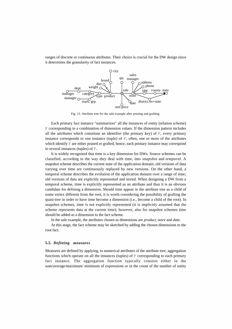
ranges of discrete or continuous attributes. Their choice is crucial for the DW design sinceit determines the granularity of fact instances.

unit price

qty

date

store

salesmanager

city state

product

brand

typecategory

addressdiet

city

weightdept.

manager

mark. grp.manager

phone

district no+state

city countysale

Fig. 13. Attribute tree for the sale example after pruning and grafting.

Each primary fact instance "summarizes" all the instances of entity (relation scheme)F corresponding to a combination of dimension values. If the dimension pattern includesall the attributes which constitute an identifier (the primary key) of F, every primaryinstance corresponds to one instance (tuple) of F; often, one or more of the attributeswhich identify F are either pruned or grafted, hence, each primary instance may correspondto several instances (tuples) of F.

It is widely recognized that time is a key dimension for DWs. Source schemes can beclassified, according to the way they deal with time, into snapshot and temporal. Asnapshot scheme describes the current state of the application domain; old versions of datavarying over time are continuously replaced by new versions. On the other hand, atemporal scheme describes the evolution of the application domain over a range of time;old versions of data are explicitly represented and stored. When designing a DW from atemporal scheme, time is explicitly represented as an attribute and thus it is an obviouscandidate for defining a dimension. Should time appear in the attribute tree as a child ofsome vertex different from the root, it is worth considering the possibility of grafting thequasi-tree in order to have time become a dimension (i.e., become a child of the root). Insnapshot schemes, time is not explicitly represented (it is implicitly assumed that thescheme represents data at the current time); however, also for snapshot schemes timeshould be added as a dimension to the fact scheme.

In the sale example, the attributes chosen as dimensions are product, store and date.At this stage, the fact scheme may be sketched by adding the chosen dimensions to the

root fact.

5.5. Defining measures

Measures are defined by applying, to numerical attributes of the attribute tree, aggregationfunctions which operate on all the instances (tuples) of F corresponding to each primaryfact instance. The aggregation function typically consists either in thesum/average/maximum/ minimum of expressions or in the count of the number of entity

instances (tuples). A fact may have no attributes, if the only information to be recorded isthe occurrence of the fact.

The measures determined, if any, are reported on the fact scheme. At this step, it isuseful for the phase of logical design to build a glossary which associates each measure toan expression describing how it can be calculated from the attributes of the source scheme.Referring to the sale example and to its logical scheme, the glossary may be compiled inSQL as follows:

qty sold = SELECT SUM(S.qty )FROM SALES S,TICKETS TWHERE S.tickNo = T.tickNoGROUP BY S.product,T.date,T.store

revenue = SELECT SUM(S.qty * S.unitPrice )FROM SALES S,TICKETS TWHERE S.tickNo = T.tickNoGROUP BY S.product,T.date,T.store

no. of customers = SELECT COUNT(*)FROM SALES S,TICKETS TWHERE S.tickNo = T.tickNoGROUP BY S.product,T.date,T.store

At this point, the aggregation functions more used for each combinationmeasure/dimension should be represented; if necessary, the preferred ordering ofdimensions for aggregation should be specified.

5.6. Defining hierarchies

The last step in building the fact scheme is the definition of hierarchies on dimensions.Along each hierarchy, attributes must be arranged into a quasi-tree such that a -to-onerelationship holds between each node and its descendants.

The attribute tree already shows a plausible organization for hierarchies; at this stage,it is still possible to prune and graft the quasi-tree in order to eliminate irrelevant details.It is also possible to add new levels of aggregation by defining ranges for numericalattributes; typically, this is done on the time dimension. In the sale example, the timedimension is enriched by introducing attributes month, quarter, etc.

During this phase, the attributes which should not be used for aggregation but onlyfor informative purposes may be identified as non-dimension attributes (for instance,address, weight, etc.). It should be noted that non-numerical attributes which are childrenof the root but have not been chosen as dimensions must necessarily either be grafted (ifthe granularity of the primary fact instances is coarser than that of the fact) or berepresented as non-dimension (if the two granularities are equal).

6. Conclusion

In this paper we have proposed a conceptual model for data warehouse design and a semi-automated methodology for deriving it from the documentation describing the informationsystem of the enterprise. The DFM is independent of the target logical model(multidimensional or relational); in order to bridge the gap between the fact schemes andthe DW logical scheme, a methodology for logical design is needed. As in operationalinformation systems, DW logical design should be based on an estimate of the expectedworkload and data volumes. The workload will be expressed in terms of query patterns andtheir frequencies; data volumes will be computed by considering the sparsity of facts andthe cardinality of the dimension attributes.

Our current work is devoted to developing the methodology for logical design andimplementing it within an automated tool. Among the specific issues we areinvestigating, we mention the following:

• Partitioning of the DW into integrated data marts.• View materialization. This problem involves the whole dimensional scheme; in fact,

due to the presence of drill-across queries, cross-optimization must be carried out.• Selection of the logical model. Each materialized view can be mapped on the logical

level by adopting different models (star scheme, constellation scheme, snowflakescheme).

• Translation into fact and dimension tables. The fact and dimension tables are createdaccording to the logical models adopted.

• Vertical partitioning of fact tables. The query response time can be reduced byconsidering the set of measures required by each query.

• Horizontal partitioning of fact tables. The query response time can be reduced byconsidering the selectivity of each query.

References

1 . R. Agrawal, A. Gupta and S. Sarawagi, Modeling multidimensional databases, IBMResearch Report, IBM Almaden Research Center, 1995.

2 . E. Baralis, S. Paraboschi and E. Teniente, Materialized view selection in multidimensionaldatabase, Proc. 23rd Int. Conf. on Very Large Data Bases, Athens, Greece, 1997, 156-165.

3 . R. Barquin and S. Edelstein, Planning and Designing the Data Warehouse. (Prentice Hall,1996).

4 . L. Cabibbo and R. Torlone, A logical approach to multidimensional databases, eds. H.J.Schek, F. Saltor, I. Ramos, G. Alonso, Advances in DB technology - EDBT 98, (LNCS1377, Springer, 1998) 183-197.

5 . S. Chaudhuri and U. Dayal, An overview of data warehousing and OLAP technology,SIGMOD Record 26, 1 (1997) 65-74.

6 . S. Chaudhuri and K. Shim, Including group-by in query optimization, Proc. 20th Int. Conf.on Very Large Data Bases (1994) 354-366.

7 . G. Colliat, OLAP, relational and multidimensional database systems, SIGMOD Record 25,3 (1996) 64-69.

8 . C. Fahrner and G. Vossen, A survey of database transformations based on the Entity-Relationship model, Data & Knowledge Engineering 15, 3 (1995) 213-250.

9 . U.M. Fayyad, G. Piatetsky-Shapiro and P. Smyth, Data mining and knowledge discoveryin databases: an overview, Comm. of the ACM 39, 11 (1996).

10. M. Golfarelli, D. Maio and S. Rizzi, Conceptual design of data warehouses from E/Rschemes, Proc. Hawaii International Conference on System Sciences, Kona, Hawaii (1998)334-343.

11. J. Gray, A. Bosworth, A. Lyman and H. Pirahesh, Data-Cube: a relational aggregationoperator generalizing group-by, cross-tab and sub-totals, Technical Report MSR-TR-95-22, Microsoft Research, 1995.

12. A. Gupta, V. Harinarayan and D. Quass, Aggregate-query processing in data-warehousingenvironments, Proc. 21th Int. Conf. on Very Large Data Bases, Zurich, Switzerland(1995).

13. H. Gupta, V. Harinarayan and A. Rajaraman, Index selection for OLAP, Proc. Int. Conf.Data Engineering, Binghamton, UK (1997).

14. M. Gyssens and L.V.S. Lakshmanan, A foundation for multi-dimensional databases, Proc.23rd Int. Conf. on Very Large Data Bases, Athens, Greece (1997) 106-115.

15. V. Harinarayan, A. Rajaraman and J. Ullman, Implementing Data Cubes Efficiently, Proc.of ACM Sigmod Conf., Montreal, Canada (1996).

16. T. Johnson and D. Shasha, Hierarchically split cube forests for decision support:description and tuned design, Bullettin of Technical Committee on Data Engineering 20, 1(1997).

17. R. Kimball, The data warehouse toolkit (John Wiley & Sons, 1996).18. D. Lomet and B. Salzberg, The Hb-Tree: a multidimensional indexing method with good

guaranteed performance, ACM Trans. On Database Systems 15, 44 (1990) 625-658.19. F. McGuff, Data modeling for data warehouses, http://members.aol.com/fmcguff

/dwmodel/dwmodel.htm (1996).20. P. O'Neil and G. Graefe, Multi-table joins through bitmapped join indices, SIGMOD

Record 24, 3 (1995) 8-11.21. K. Ross, D. Srivastava and D. Chatziantoniou, Complex aggregation at multiple

granularities, Proc. Int. Conf. on Extending Database Technology (1998) 263-277.22. S. Sarawagi, Indexing OLAP data, Bullettin of Technical Committee on Data Engineering

20, 1 (1997).23. Y. Zhuge, H. Garcia-Molina and J. L. Wiener, The Strobe Algorithms for Multi-Source

Warehouse Consistency, Proc. Conference on Parallel and Distributed InformationSystems, Miami Beach, FL (1996).