The Direct Primary and

Candidate-Centered Voting

in U.S. Elections

May, 2012

Abstract

In this paper we document a strong correlation between the use of primaries and the tran-

sition from “party-based” voting to “candidate-oriented” voting in U.S. statewide elections.

First, at the aggregate level we find that the direct primary is associated with a significant

increase in “split-ticket” voting, both across states and within states over time. Second,

we use a new data set of county level primary election returns to examine the relationship

between primary and general election voting patterns. We find that general election candi-

dates gather more votes in counties where they received relatively high electoral support in

the primaries, even after taking into account election-specific factors and the “normal vote”

across counties. We also provide some evidence that primary competition may affect the

salience of particular candidate attributes in general election outcomes. [Word count 10865]

1. Introduction

U.S. elections today are relatively “candidate-centered” contests. This is true not only

compared to the “party-centered” elections in western Europe and many other countries,

but also compared to U.S. elections in the past.

When and why did this era of more personalistic voting emerge? Currently, the con-

ventional wisdom is that U.S. elections became much more candidate-centered around the

1960s. Aldrich and Niemi (1990) refer to the post-1960s era as the “the sixth party system.”

Aldrich (1995, p. 253) summarizes the literature as follows:1

Together these studies show that there was an important shift in elections to all

national offices in or about 1960, demonstrating that voters respond to candidates

far more than previously. Voting became candidate centered, and so parties as

mechanisms for understanding candidates, campaigns, and election became less

relevant.

The change from partisan to personal electoral politics is generally attributed to changes

in the political environment that increased the salience of individual politicians’ attributes

and weakened traditional party organizations – changes in campaign advertising technologies

such as the rise of television, the replacement of patronage with civil service employment, and

an increase in the personal resources available to elected officials for constituency service.

These factors led voters to see parties as increasingly irrelevant, and party attachments

weakened. Campbell (2007, p. 68) describes the process as follows:

Since the 1960s the role of the political parties in American politics has fundamen-

tally changed. A series of technological, institutional, legal, and cultural shifts

diminished their once central function as the organizers and inclusive mobiliz-

ers of American elections. They ceded control over nominations and were pushed

aside by new candidate-centered campaigns. Technological advances allowed can-

didates to speak directly to the people, and the parties lost their monopoly.

1Aldrich cites numerous articles and books, including Nie, Verba and Petrocik (1979), Alford and Brady(1989), Wattenberg (1990, 1991), Jacobson (1992), and Shively (1992). Some recent literature argues thatpersonal voting, based on incumbency and quality, may have had a role in electoral even the strong partyera prior to the 1890s (e.g. Carson, et. al. 2007; Reynolds, 2006).

2

An earlier literature emphasizes the potential for institutional factors – such as the Aus-

tralian ballot, ballot form (e.g. straight party lever, office-bloc vs. party-list), and direct

primaries – to weaken party-centered voting and transition towards candidate-centered vot-

ing. Rusk (1970) finds that the split-ticket voting increased in states that adopted the

Australian ballot, and the increase was especially large in states with office-bloc ballots and

no party lever.2 Campbell and Miller (1957) also find that ballot form influences split-ticket

voting using survey data. As Campbell et. al. (1960) state in The American Voter, “Any

attempt to explain why the voter marks a straight or split ballot must take account of the

physical characteristics of the election ballot.”

Regarding direct primaries, Key (1964, p. 342) writes that “the adoption of the direct

primary opened the road for disruptive forces that gradually fractionalized the party organi-

zation. [T]he primary system... facilitated the construction of factions and cliques attached

to ambitions of individual leaders.”3 Some more recent scholars make similar arguments. For

example, Herrnson (1988, p. 26) writes: “The introduction of the direct primary encouraged

candidates to develop their own campaign organizations, or pseudo-parties, for contesting

primary elections.” Jacobson (2004, p.15-16) emphasizes the impact this has had on party

organizations:

A fundamental factor [in the decline of parties] is clearly institutional: the rise

and spread of primary elections as the method for choosing party nominees for the

general election... Primary elections have largely deprived parties of their most

important source of influence over elected officials. Parties no longer control

access to the ballot and, therefore, to political office. They cannot determine

who runs under their label and so cannot control what the label represents...

parties typically have few sanctions and little influence [on nominations].”

The argument that the introduction of direct primaries increased the electoral salience

of non-partisan factors in the U.S. is also consistent with the conventional wisdom in the

comparative politics literature that electoral institutions are crucial in determining the degree

2Burnham (1965) also finds an increase in split-ticket voting around this period but does not link thechanges to any specific electoral institutions.

3As cited in Miller, Jewell and Sigelman (1988, p. 459).

3

to which elections are candidate- versus party-centered. In particular, institutions that

promote intra-party competition provide incentives for candidates to cultivate “personal

votes” separate from their partisan affiliation in order to compete against co-partisans (e.g.

Carey and Shugart, 1993).

While many observers suspect that primary elections may contribute to making elections

more candidate-centered, there is little systematic evidence directly linking primary compe-

tition to the electoral salience of non-partisan candidate attributes in the general election. A

large empirical literature examines the effect of primary election competition on general elec-

tion outcomes for non-presidential elections with mixed results.4 Most of the studies which

find an effect of primaries on general election outcomes focus on the post-1960 candidate-

centered election period. However, most states passed legislation making primary elections

mandatory several decades prior to the widely discussed rise in personal voting that occurred

in the middle of the 20th century. Thus, whether primary elections are actually connected

to candidate-centered voting remains an open question.

There is an important theoretical difference between the direct primary and ballot-related

explanations for candidate-centered voting. The effects of ballot form could largely occur

in the polling booth at the time voting. A party lever or circle clearly lowers the cost

of casting a straight party ballot. Prior to the Australian ballot, party ballots were often

printed in ways that made it difficult for a voter to split their ticket and allowed party

workers to monitor voting behavior (e.g. Bensel, 2004). In contrast, the effects of the

direct primary on candidate-centered voting, if any, operate earlier during the campaign

period. As noted above, scholars argue that the direct primary weakened party organizations

creating strong incentives for candidates to develop their own organizations for the primary

and general election campaigns. These changes likely increased the salience of candidates’

personal attributes – e.g. issue positions, charisma, ethnicity, gender – in both the primary

and the general election. This would potentially link the voting behavior in the two elections.5

4For example, Born (1981), Kenney and Rice (1984), and Romero (2003) find some evidence that divisiveprimaries affect general election outcomes. Hacker (1965) and Kenney (1988) find little evidence that divisiveprimaries have an effect on general election voting. Ware (1979) discusses why primaries may not necessarilyhave a negative effect on candidates’ general election prospects.

5In addition to direct effects on election day, changes in ballot laws may have also had important indirect

4

In this paper we examine the connection between primary competition and candidate-

centered voting in U.S. elections. This is the first study, at least to our knowledge, that

provides evidence that primary competition is related to the salience of candidate attributes

in general elections, and, moreover, that this relationship existed even in the decades before

the era of candidate-centered voting emphasized in the current literature.

We focus on three questions: (1) Is there any association between the growth of “candidate-

centered” voting, as measured by split-ticket voting, and the introduction of direct primaries?

(2) Are the candidate attributes affecting primary elections also affecting the personal vote

in general elections even prior to the 1960s? (3) Does primary competition affect the degree

to which the attributes salient in the primaries are also salient in the general elections?

To address the first question, we examine whether personal voting increased in a given

state around the time when that state adopted direct primary elections. For this analysis we

use “split-ticket voting” to indicate the degree to which votes were cast based on candidates’

personal characteristics rather than on partisan attachments. We use aggregate voting re-

turns across statewide elected offices to construct a crude measure of “split-ticket voting”

for each state and year from 1876 to 2006. Analyzing this measure, we find clear evidence of

a “transition period” in the first half of the 20th century – from about 1890 to 1920 – during

which the degree of split-ticket voting rose sharply in those states that adopted a compre-

hensive, mandatory primary. The timing of the changes, both across states and within state

over time, suggests that primaries played a prominent role in this first transition. This also

allows us to assess the relative importance of primary elections compared to ballot form in

accounting for increases in split-ticket voting. We find that the estimated effect of the direct

primary is at least as large as the effect of the straight party lever/circle.

The second question concerns whether the specific attributes salient in primaries are

related to personal voting in general elections. This would provide further evidence con-

necting the direct primary to candidate-centered elections. For this analysis we examine

whether the areas where candidates receive electoral support in the primary are also the

areas where their general election vote shares are above what would be expected given the

effects, weakening party organizations and inducing more candidate focused campaigns. To our knowledge,there is no systematic evidence for these indirect effects.

5

election-specific factors and the normal vote in the areas. Such an association suggests that

the specific candidate attributes salient in the primary are also salient in the general elec-

tions. We exploit a new data set of county level primary and general election returns from

1906 to 2006 to measure areas of candidate support in the primary and general election. We

find clear evidence that areas where a nominee does well in the primary election are also the

areas where the nominee does well in the general election even in the early decades of the

20th century. Thus, personal voting on the basis of candidate attributes appears to have

existed in the general elections even prior to the 1960s.

We also explore whether candidates’ personal vote varies across general elections in rela-

tion to the attributes salient in the primary elections or whether candidates’ personal votes

are relatively stable and mainly reflect the salience of certain fixed attributes of the nomi-

nees in the general elections. For this analysis we exploit cases where the same Democratic

and Republican candidates face each other in more than one general election, but they face

different challengers in the primary elections leading up to each general election. By focusing

on repeat general election nominees, we can assume that the fixed attributes of the parties’

nominees (e.g. hometown locations, gender, race) remain relatively stable across elections.

However, in the primaries the general election nominees may face different challengers who

raise the salience of different candidate attributes in each primary. We find that even after

accounting for the effect of the fixed attributes, there is still a statistically significant as-

sociation between where candidates receive support in primary and general elections. This

is further evidence consistent with what we would expect to observe if the attributes that

are salient during primary elections are also contributing to candidates’ personal vote in the

general elections.

The third question concerns the causal relationship between primary competition and

salience of particular candidate attributes in the general elections. While the evidence in

the first two sections suggest that an association exists between the direct primary and

candidate-centered politics, the analyses do not isolate the causal effect of primary compe-

tition on the salience of candidate attributes in the general election. It is possible that the

attributes salient in primary elections would be salient in the general election even if the

6

primaries did not exist.6 For this analysis we employ two different research strategies to es-

timate the impact of primary competition on the degree to which general elections focus on

personal attributes: (1) the discontinuity around the threshold for run-off elections; (2) the

difference in attention given to primary elections in safe versus competitive states. While

both strategies require making different assumptions for identification, they both provide

some tentative evidence that primary competition may influence the salience of particular

candidate attributes in the general elections.

Finally, we also provide some discussion regarding how candidate attributes for one office

may spill over to the election outcomes for other offices. In particular, we focus on whether

the attributes salient in primary elections for top-of-the-ticket offices are related to down-

ballot general elections and vice versa. We find that the counties that support the top-of-

the-ticket nominees in the primaries are also the counties where the down-ballot nominees

from the same party receive higher than expect general election vote shares, even after the

primary vote shares of the down-ballot nominees are taken into account. This relationship is

mainly prevalent in the early decades of the 20th century. These results suggest that primary

competition for top-of-the-ticket offices may have an even larger effect on electoral politics

than is suggested by the previous discussion, since the personal vote of top-of-the-ticket

candidates may influence the outcomes of the down-ballot races.

2. Primaries and “Split-Ticket” Voting

One indicator of candidate-centered voting is the degree to which the electorate engages

in“split-ticket” voting. In party-centered systems we would expect voters to vote for all of the

candidates from the same party across offices within an election. A crude measure of “split-

ticket” voting is the variation in the two-party vote across offices in a given election. This

is obviously a lower bound on the total amount of split-ticket voting, since individual voters

may split their tickets in different ways that cancel one another. However, the correlation

between split-ticket voting measured at the individual level and the aggregate-level proxies

6A common critique of studies of the effect of divisive primaries on general election outcomes is that therelationship may reflect a single shock to a candidate’s valence which would affect both their primary andgeneral election support.

7

is quite high.7

We augmented the data in Ansolabehere and Snyder (2002), Ansolabehere et al (2006),

and Ansolabehere et al (2010), to create a nearly complete data set of election returns for

all statewide races in all states for the period 1876-2008.8 For each state-year in which there

are 3 or more statewide races, we construct the variable Standard Deviation as follows:

Standard Deviation kt =1

Nkt−1[

N∑i=1

(Vjkt − V kt)2 ]1/2

where Nkt is the number of statewide races in state k in year t, Vjkt is the Democratic share

of the two-party vote in race j in state k in year t, and V kt is the average of the Democratic

percentage of the two-party vote across all races in state k in year t. We only include races

contested by both major parties, and we drop races in which a third-party candidate received

more than 15% of the total vote.

Figure 1 shows a graph of the average value of Standard Deviation in each year. The

circles are for the set of states that adopted a comprehensive, mandatory primary election

law during the period 1900-1915 and did not subsequently repeal the law, while the triangles

are for the states that did not.9

The two curves are similar, showing a small but clear increase in Standard Deviation

starting around 1900, and a larger increase between 1960 and 1980. One obvious difference

between the curves is that the early increase is noticeably larger for the states that adopted

7Using data from exit polls and the CCES we know that split ticket voting tends be higher at the individuallevel than the aggregate level differences would suggest. However the measures of split-ticket voting usingstate level data are highly correlated with measures using individual level data. Consider, for example, split-ticket voting for senate and governor for the period 1982-2006. For each state-year with both a Senate andGovernor race, let sikt be a dummy variable equal to 1 if respondent i in the exit poll voted for candidatesfrom different parties in the Senate and Governor races (including third-party and independent candidates),

and 0 otherwise; let Nkt be the number of respondents in the exit poll; and let SIkt = (1/Nkt)

∑Nkt

i=1 sikt bethe overall amount of split-ticket voting at the individual level. Let DG

kt (DSkt) be the aggregate Democratic

share of the two-party vote in the Governor (Senate) race; and let SAkt = |DG

kt−DSkt| be the aggregate measure

of “split-ticket” voting. The correlation between is SI and SA is .72 (N=157).8Statewide races include offices such as U.S. senator, governor, lieutenant governor, attorney general,

secretary of state, treasurer, auditor/comptroller/controller, superintendent of education, commissioner ofagriculture, public utility commissioner, corporation commissioner, and lands commissioner. We also includeinclude races for various statewide offices specific to certain states. See Ansolabehere and Snyder (2002),Ansolabehere et al (2006), and Ansolabehere et al (2010) for a complete list of sources and offices used inthis analysis.

9Each state is weighted equally in each year. We group the odd-numbered years together with the previouseven-numbered year – e.g., 1881 with 1880, etc.

8

a comprehensive mandatory primary, and that a large gap opens between these states and

states without primaries starting around 1918. This is intriguing because, as noted above,

the period 1900-1915 was the era in which most states adopted their primary laws.Standard Deviation

Stan

dard

Dev

iati

on

Standard DeviationYear

Year

Year Mandatory Primary States

Mandatory Primary States Non-Primary States

Non-Primary States1880

1880

18801900

1900

19001920

1920

19201940

1940

19401960

1960

19601980

1980

19802000

2000

20000

0

02

2

24

4

46

6

68

8

810

10

10

Figure 1. The circles represent the standard deviation of the statewide office vote sharesfor states that introduced mandatory direct primaries between 1900 and 1915. The trianglesrepresent the states that introduced mandatory direct primaries after 1915.

For the states adopting a comprehensive mandatory primary there are three “plateaus,”

one from about 1876 to 1900, another from about 1920-1958, and a third from about 1972-

2006. The average value of Standard Deviation during the first plateau is 0.9, the average

value in the second plateau is 3.3, and the average value in the third plateau is 7.8. Thus,

for these states the shift from the first period to the middle period was about 35 percent of

the total change between the first period and the third, clearly a non-trivial change.10

Regression analyses shows that the differences in split-ticket voting between the primary

10Calculated as follows: 100(3.3 - .9)/(7.8 - .9) = 34.7.

9

and non-primary states is statistically significant and substantively important. In these anal-

yses we can also compare the relative importance of primary elections and other institutional

factors, such as ballot form. The results are shown in Table 1. The independent variables

are: Direct Primaryst =1 if state s employed primary elections in year t; Straight Ticketst =

1 if state s had a straight party lever/circle on the ballot in year t; Office Blockst = 1 if state

s used the office block ballot form in year t; Party Listst = 1 if state s used the party list

ballot form in year t; Log Total Votest is the logarithm of the total vote in state s and year

t.11 Note that the coefficients on the two ballot form variables, i.e. Office Block and Party

List, are relative to the excluded category, which is the pre-Australian ballot “party ballot”.

Table 1Primaries and Split-Ticket Voting, 1876-2009

1 2 3 4 5 6

Direct Primary 1.60 1.14 1.20 1.49 1.36 1.34(0.49) (0.44) (0.44) (0.41) (0.39) (0.38)

Straight Ticket -1.79 -1.38 -0.71 -0.70(0.40) (0.36) (0.50) (0.48)

Office Block 0.89 0.99 0.36 0.38(0.72) (0.64) (0.50) (0.50)

Party List 1.08 0.80 0.26 0.25(0.77) (0.71) (0.64) (0.62)

Log Total Vote -0.52 -0.34(0.11) (0.40)

State FE & State Trends No No No Yes Yes Yes

Observations 1,771 1,771 1,771 1,771 1,771 1,771

Year fixed effects included in all specifications. Standard errors are in parentheses. Standarderrors are clustered by state in all specifications.

In columns 2, 3, 5, and 6 we include indicators for differences in ballot form, such as

whether there is an easy option to vote a straight party ticket or whether candidates are

11We also ran specifications including measure party competition. This variable was never statisticallysignificant and did not substantively change the coefficient estimates on our main variables of interest.

10

grouped by office or party, that are often argued to affect split-ticket voting.12 When state

fixed effects and state trends are included in the regression, only the introduction of primary

elections appears to be associated with a statistically significant change in split ticket voting.

When fixed effects and time trends are not included, the direct primary is found to have a

similar effect on split-ticket voting as whether a straight party ticket option is included on

the ballot.13

This analysis does not necessarily demonstrate that the adoption of a mandatory primary

law caused an increase in Standard Deviation. For example, the decline of “strong party

organizations” might be the real cause of the increase in split ticket voting. Strong party

organizations might have prevented the adoption of primary laws in their states and might

also have reduced the amount of split-ticket voting. Of course, since the analysis includes

state and year fixed-effects it must be that party organizational strength changed within

states over time and in different states at different times (i.e., not as the result of a nationwide

shock such as a transformative presidential election). A plausible alternative explanation of

the pattern is that party organizations might have weakened in some but not all states

during the 1900s, leading the affected states to adopt a primary law and also to experience

an increase in split-ticket voting.

Nonetheless, the analysis above does establish two things: (1) there was a significant

increase in “split-ticket” voting much earlier than the conventional wisdom suggests; and (2)

this increase was especially noticeable in states that adopted a comprehensive mandatory

primary between 1900 and 1915.

3. Candidate Attributes in Primary and General Elections

In this section we examine whether personal voting is related to the candidate attributes

that affected the primary election outcomes for the general election nominees. We use a new

dataset of county-level primary election returns from 1906 to 2006 to provide evidence that

the candidate attributes which affect primary election outcomes also affect general election

12See for example Ansolabehere et. al. (2007) and Harvey and Mukherjee (n.d.).13We find no statistically significant evidence that the introduction of the Australian ballot is associated

with an increase in split-ticket voting. The estimated coefficients on the ballot form variables are particularlysensitive to choice of time period and specification.

11

outcomes. With this new dataset we can exploit the presence of multiple observations

for the same primary candidates within elections and multiple observations for the same

county across elections. This allows us to examine whether the areas where general election

candidates had higher-than-expected vote shares are also the areas where these candidates

had relatively high vote shares in the primary election.

3.1 Data and Methods

We assembled a new dataset of county-level primary election returns for the period 1906

to 2006. We collected much of the historical data on primary electoral returns from state

legislative manuals and various official state reports of primary and general election returns.

We also incorporated information for senatorial and gubernatorial elections in southern states

between 1920 and 1972 from two ICPSR datasets (I00072 and I00071). Although the dataset

does not cover all primary elections for every state during the period under investigation,

we do include elections from forty-seven states over the period 1906 to 2006.14 We merge

this primary data with county-level general election data. For most of this paper we focus

on senate and gubernatorial elections since we have almost all county-level general election

data for the period until 2006 from an updated version of ICPSR I0001 and have been able

to collect most county-level primary elections data for this same period.15

We also gathered county level primary and general election returns for down-ballot

statewide offices for the forty-three states that had down-ballot elections.16 This dataset in-

cludes election returns for lieutenant governor, secretary of state, treasurer, auditor, comptroller,

and attorney general. Part of these data comes from ICPSR 7861. We gathered the remain-

ing data from state legislative manuals. This dataset is not as comprehensive as the dataset

for governors and senators as we are still missing the county level primary and/or general

election results for a number of the down-ballot elections.

Following the literature we assume that the county-level election outcomes are determined

by factors specific to local areas (e.g., partisanship), candidate-specific characteristics (e.g.,

14Alaska, Hawaii and Connecticut are not included in this analysis.15Data for the 2004 and 2006 Senate election data were purchased from http://uselectionatlas.org.16Maine, New Hampshire, New Jersey and Tennessee do not have primary elections for the down-ballot

offices included in this study.

12

quality and incumbency), and contest-specific factors (e.g., salient issues in a particular

campaign). Thus, the vote share of the Democratic candidate in county i of electoral contest

j can be written as follows:

Vij = Ni +QDj +QR

j + θ1ADij + θ2A

Rij + Zj + εij (1)

where Ni is the partisanship of county i. QDj and QR

j are characteristics of candidates

that affect their vote share evenly throughout the district. We might think of this as the

overall quality of the candidate or the incumbency advantage. ADij and AR

ij are non-partisan

attributes of the Democratic and Republican candidates that affected their support in county

i in the primary election leading up to general election contest j. Zj captures partisan tides,

or other factors such as specific issues, that have the same effect across all counties in race

j.

Unfortunately we cannot directly measure county partisanship, Ni, for much of the period

we are studying. However, if we assume that county partisanship does not vary significantly

across elections within decades, then we can account for this and other time invariant county

features with county fixed effects that vary by decade. Similarly, QDj , QR

j and Zj are also

difficult to measure directly so again we assume that these factors do not vary across counties

within districts. This allows us to capture these race-specific characteristics with race-specific

fixed effects.

Although we cannot directly observe the candidate attributes that appeal to primary and

general election voters, we can observe the variation in areas where the candidates received

support in the primary election. Since primary voters presumably make decisions based

upon candidate-specific attributes separate from their partisan affiliation, we would expect

candidates’ primary vote shares to be a proxy for support for particular candidate attributes

in a particular county.

Thus, the basic specification we estimate is as follows:

Vij = αi + γj + θ1PDij + θ2P

Rij + εij (2)

The dependent variable, Vij, is the general election vote share of the Democratic Party can-

13

didate in county i and race j.17 αi is a fixed effect for county i, which captures characteristics

of county i such as partisanship. αi varies by decade. γj is a fixed effect for contest j which

captures contest-specific factors such as the quality of the candidates running in contest j.

PDij and PR

ij are measures of the Democratic and Republican nominees’ vote share of the top

two candidates in the primary election preceding general election contest j.

If candidate attributes which affect primary election outcomes are also salient in the

general election, then we would expect θ1 to be positive and θ2 to be negative. We examine

whether this relationship exists for both top-of-the-ticket offices, i.e. governor and senator,

as well as down-ballot offices. We might expect the relationship to be stronger for top-of-

the-ticket races since the candidates in these races tend to receive more resources and media

attention to cultivate their personal vote. We also allow θ1 and θ2 to vary over time to

examine whether the relationship between these candidate-specific attributes and general

election outcomes is mainly in the post-1960 era as we would expect if elections became

candidate-centered during this period.

3.2 Results

The results in Table 2 provide evidence that the candidate attributes which affect primary

election outcomes also appear to influence general election outcomes. The top panel of Table

2 includes all states and all offices. The results in column 1 in this panel, which includes all

years, finds that on average, the areas where candidates do well in primary election are also

areas where the candidates do better than expected in the general election. If the Democratic

(Republican) nominee’s primary vote share is 40 percentage points higher in county A as

compared to county B, then, on average, the nominee’s general election vote share is about

2.8 (2.4) percentage points higher in county A compared to B.18

We also estimate separate θ1 and θ2 for top-of-the-ticket and down-ballot offices. The

results for the top-of-the-ticket (down-ballot) offices are in the second (third) panel of Table

17We excluded uncompetitive general election races – i.e. races where the Democratic or Republicancandidate received more than 95% of the vote. The main results do not substantive change when these racesare not excluded.

18The standard deviation of the Democratic and Republican nominee’s county level primary percentagevote share of the top two candidates is about 18.

14

2. The association between the county level primary and general election returns is stronger

for governors and senators relative to down-ballot offices. If the Democratic (Republican)

senatorial or gubernatorial nominee’s primary vote share is 40 percentage points higher in

county A as compared to county B, then, on average, the nominee’s general election vote

share is about 3.6 (3.2) percentage points higher in county A compared to B. For down-ballot

offices nominees a 40 percentage point higher vote share in the primary election is associated

with a 1.2 (1.6) percentage point higher vote share in the general election.

Table 2Primary Electoral Support and General Election Outcomes

All Pre-1960 Post-1960

All Offices

Dem Nominee Primary Support 0.07 0.06 0.09(0.01) (0.01) (0.01)

Rep Nominee Primary Support -0.06 -0.06 -0.07(0.01) (0.01) (0.01)

Observations 252194 134091 118103

Governor and Senator

Dem Nominee Primary Support 0.09 0.08 0.11(0.01) (0.01) (0.01)

Rep Nominee Primary Support -0.08 -0.08 -0.09(0.01) (0.02) (0.01)

Observations 137121 68490 68631

Down-ballot Offices

Dem Nominee Primary Support 0.03 0.02 0.06(0.01) (0.01) (0.01)

Rep Nominee Primary Support -0.04 -0.03 -0.04(0.01) (0.01) (0.01)

Observations 115073 65601 49472

The dependent variable is the county level general election Democratic vote share of theDemocratic and Republican vote. State-county fixed effects that vary by decade are in-cluded in all regressions. Race specific effects are also accounted for in all of the regressions.Standard errors clustered by state are in parentheses.

15

While the larger estimates of θ1 and θ2 for the top-of-the-ticket as compared to down-

ballot offices may be determined by a number of alternative factors, one likely explanation

for the difference is that voters have more exposure to information about candidates for

top-of-the-ticket offices either through the media or the election campaigns. We know, at

least in the recent period, that top-of-the-ticket primary candidates have significantly more

newspaper mentions in the months prior to the primary election as compared to down-ballot

candidates.19

Another question of interest is whether the candidate attributes that affect primary

election outcomes became even more salient in the post-1960 general elections. Column 2 of

Table 2 includes all elections prior to and including 1960. Column 3 includes all elections

post-1960. The results in these two columns suggest that the candidate attributes salient

in the primary elections were related to general election outcomes even prior to the 1960s.

However, the relationship between primary and general election voters is particularly strong

for Democrats in the post-1960 period – i.e. θ̂1 is substantially larger in the post 1960 period

relative to the pre-1960 period.

Figure 2 plots the estimates of θ1 and -θ2 for senatorial and gubernatorial candidates

by decade. This figure again illustrates that the association between primary and general

election outcomes existed even in the early decades of the 20th century. Both θ̂1 and θ̂2

appears to have increased in magnitude in the 1970s, 80s and 90s around the same time as

there was a growth in the incumbency advantage. This is also the period when scholars claim

elections became more candidate-centered. The coefficient estimate on Democratic primary

support, θ̂1, seems to have started to increase in magnitude in the 1960s, which is perhaps

not surprising given the divisions in the Democratic party during this decade. The slightly

larger coefficient for the Republicans during the early decades is also consistent with the

historical accounts of deep divisions within the Republican party between the progressive

and stalwart factions. Somewhat surprising is the decline in magnitude of θ̂1 between the

19We examined the number of times primary candidates were mentioned relative to the word electionduring the months prior to a primary election in the newspapers included in newslibrary.com during theperiod 1998 to 2006. The top-of-the-ticket candidates received significantly more newspaper mentions relativeto the down-ballot candidates.

16

1970s the 2000s.20

D

D DD D

D

D

D

D

D

R

R

R RR R

R

R R

R

0.0

2.0

4.0

6.0

8.1

.12

.14

.16

Coe

ffici

ent o

n P

rimar

y S

uppo

rt

1910 1920 1930 1940 1950 1960 1970 1980 1990 2000Decade

Figure 2. Results By Decade.

Figure 3 plots separate estimates of θ1 and -θ2 by decade for incumbent and non-

incumbent senatorial and gubernatorial candidates. In general the coefficient estimates for

both incumbent and non-incumbent candidates tend to be larger in the later part of the

century, which is consistent with a general rise in candidate-centered voting in the latter half

of the century. The coefficient estimates for Republican candidates do not exhibit the same

dramatic growth around the 1960s as is seen for the Democrats. This again may be related

to the internal divisions between the progressive and stalwart factions within the Republican

party, particularly in the midwestern states, during the earlier decades of the century.

20One conjectures is that this decline may be related to the rise in polarization. What is driving thisdecline in θ̂1 remains an open research question.

17

d

d dd

dd

dd

d

d

DIDI

DI

DI

DI

DI

DI DIDI DI

r

r rr r r

r rr

rRI

RI

RI

RI

RI

RI

RI

RI

RI RI

0.0

5.1

.15

.2.2

5.3

Coef

ficie

nt o

n Pr

imar

y Su

ppor

t

1910 1920 1930 1940 1950 1960 1970 1980 1990 2000Decade

Figure 3. Results By Decade and Incumbency Status. d and r represent the coefficientestimates on the primary vote for non-incumbent Democrats and Republicans respectively.DI and RI represent the coefficient estimates on the primary vote for incumbent Democratsand Republicans respectively. The coefficients for Republicans are multiplied by -1.

The more striking feature of Figure 3 is the substantially larger estimates of θ1 and -θ2

for incumbent candidates especially in the latter half of the century. This difference may

in part reflect the gap in the amount of information primary voters have about the two

types candidates. Like candidates for top-of-the-ticket offices, incumbents in general are

given more media coverage and campaign resources. The difference may also reflect the

selection of races where incumbents face primary challenges. Since incumbents, especially

in the latter half of the century, are less likely to face primary challenges (Ansolabehere, et.

al. 2010), when they do face a primary competition it may indicated the presence of some

deep intra-party division or particularly salient candidate attribute.

We can also examine how θ1 and θ2 vary by state. Figure 4 plots the estimates of

θ1 and θ2 for all offices and years by state. We see that the estimates of θ1 and θ2 have

the expected signs – i.e. θ̂1 > 0 and θ̂2 < 0.21 Thus, in all states both Democratic and

21LA is dropped because only a small sample of races have competitive general elections and partisanprimaries. DE is dropped because of the small number of counties.

18

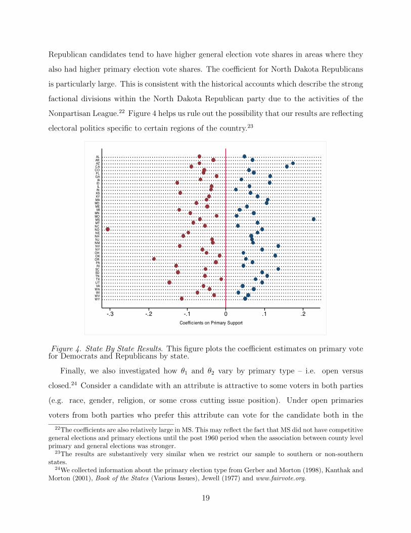
Republican candidates tend to have higher general election vote shares in areas where they

also had higher primary election vote shares. The coefficient for North Dakota Republicans

is particularly large. This is consistent with the historical accounts which describe the strong

factional divisions within the North Dakota Republican party due to the activities of the

Nonpartisan League.22 Figure 4 helps us rule out the possibility that our results are reflecting

electoral politics specific to certain regions of the country.23

-.3 -.2 -.1 0 .1 .2Coefficients on Primary Support

WYWVWI

WAVAUTTXTNSDSCRIPA

OROKOHNYNVNMNJNHNENDNCMTMSMOMN

MIMEMDMAKYKSINILIDIA

GAFL

COCAAZARAL

Figure 4. State By State Results. This figure plots the coefficient estimates on primary votefor Democrats and Republicans by state.

Finally, we also investigated how θ1 and θ2 vary by primary type – i.e. open versus

closed.24 Consider a candidate with an attribute is attractive to some voters in both parties

(e.g. race, gender, religion, or some cross cutting issue position). Under open primaries

voters from both parties who prefer this attribute can vote for the candidate both in the

22The coefficients are also relatively large in MS. This may reflect the fact that MS did not have competitivegeneral elections and primary elections until the post 1960 period when the association between county levelprimary and general elections was stronger.

23The results are substantively very similar when we restrict our sample to southern or non-southernstates.

24We collected information about the primary election type from Gerber and Morton (1998), Kanthak andMorton (2001), Book of the States (Various Issues), Jewell (1977) and www.fairvote.org.

19

primary and the general election. In contrast, under closed primaries voters who have the

opposite partisan affiliation from the candidate with the preferred attribute cannot easily

“cross-over.” Thus, many more voters who favor that candidate in the general election

will be able to vote for this candidate in the primary. As a result, one might expect that

the correlation between voting in the primary and general election will be higher under

open primaries. In fact, we find no robust and statistically significant evidence that the

magnitudes of the estimated coefficients are related to primary type.

3.3 Repeat Challengers

While the above results suggest that county-level primary and general election outcomes

are correlated, we would also like to know whether this correlation mainly reflects the salience

of fixed attributes of the general election candidates, such as race, gender, hometown loca-

tions, which are present irrespective of who the nominees face in their primaries, or whether

this correlation also reflects the specific attributes that are made salient in particular primary

elections. If primary and general election support are still correlated even after taking into

account the fixed attributes of the general election candidates, then this would suggest that

the candidate specific attributes raised during primary elections are at least related to the

personal vote in the general elections.

To examine whether the above result is largely capturing the salience of the fixed at-

tributes of general election candidates, we focus on cases with repeat general election chal-

lengers who face different challengers during their primary elections. Since the fixed at-

tributes are the same for repeat challengers, we can examine whether the variation in pri-

mary election support still has an effect on general election outcomes even when we account

for these fixed attributes. To further minimize the possibility that the issues raised in the

primaries affects the general election campaign strategies, we also examine cases where candi-

dates face repeated uncontested general elections but variation in their primary competition.

The intuition behind the identification strategy is relatively straightforward. Suppose

that two candidates A and B compete against each other in two different general elections,

one a time t and the second at time t+ 1. Candidates A and B each face different primary

20

challenges to be their party’s general election nominees at times t and t+1. If the coefficients

in the above analyses are simply reflecting the effect of fixed attributes of A and B that have

the same salience across elections, then we would expect candidates A and B’s electoral

support at times t and t+1 to come from the areas that are attracted to their fixed attributes

– i.e. the same areas should be supporting A and B in both general elections. However,

if different candidate attributes are salient in the different primary elections then we might

expect differences in candidate A’s time t and t + 1 primary vote shares to be associated

with differences in her general election vote shares in the corresponding periods.

If we assume that the salience of all the general election candidates’ attributes remain

completely fixed across the general election campaigns, then this could be considered evidence

regarding whether primary competition influences general election outcomes. As in the above

analysis, it is still possible that the salience of a particular attribute in the general election

could change even though the nominees remain the same. Thus, we cannot rule out the

possibility that the variation in the salience of particular candidate attributes was not a

result of the primary competition and would have affected the general election outcomes even

in the absence of the primary competition. However, an association between the primary

outcomes and general election outcomes even after accounting for fixed attributes of general

candidates at least suggests that at least a portion of candidates’ personal votes does vary

across elections. This raises the possibility that primary competition could affect the salience

of particular candidate attributes in the general elections.

As in equation (1) above, the county-level votes shares of the Democratic candidate in

county i of general election contest j are determined by factors specific to local areas (e.g.,

partisanship), candidate-specific characteristics (e.g., quality and incumbency), and contest-

specific factors (e.g., salient issues in a particular campaign). However, now we assume

that for every pair of general election candidates, k, there are some fixed attributes of the

candidates, F , and some attributes that vary across elections, A. Equation (1) can be

rewritten as follows:

Vijk = Ni +QDj +QR

j + θ1FDik + θ2A

Dijk + θ3F

Rik + θ4A

Rijk + Zj + εijk (3)

As above, the specification is simplified, but in this case we include county fixed effects that

21

vary by pairs of general election candidates, αik. Thus, the specification we estimate is:

Vijk = αik + γj + θ2PDijk + θ4P

Rijk + εijk (4)

If there is variation in the salience of candidate attributes across elections that affects both

the primary and general election outcomes then we would expect θ2 > 0 and θ4 < 0.

The results in the first two columns of Table 3 provide further evidence that the salience

of particular candidate attributes varies across elections and the salience is associated with

both the primary and general election outcomes. Column (1) contains races for all offices

and column (2) focuses on senate and gubernatorial races. These first two columns only

include races with contested general elections – i.e. both a Republican and a Democratic

candidate. The coefficient estimates are statistically significant with the expected sign, which

suggests that the results in the above section are not solely capturing the salience of fixed

attributes of the general election candidates. The magnitude of the estimates are slightly

larger when the sample is restricted to senate and gubernatorial elections. The estimates

of θ2 and θ4 in column (2) suggest that on average a 40 percentage point difference in

the Democratic (Republican) senate or gubernatorial candidates’ primary vote share across

counties is associated with a 2.4 (1.6) percentage point difference in general election votes.

This is a smaller effect than was estimated in the above section.

In the above specification, it is possible, and perhaps likely, that the primary election

competition may be correlated with changes in the content of the general election campaigns

even when the party nominees have not changed. In columns (3)-(5) of Table 3 we focus on

cases where the same candidate competes in multiple uncontested general elections. In these

cases there is likely to be less variation in the general election campaign strategies across the

years. Uncontested elections also tend to be in states where one political party is dominant

so the primary elections may be given relatively more attention in these races. We use the

same specification as in equation (4), but now the dependent variable is the Democratic

(Republican) vote divided by the voting age population.

The results in columns (3) and (4) suggest that Democratic nominees’ primary vote

shares are positively correlated with general election turnout, even after accounting for the

influence of the nominees’ fixed attributes. This relationship exists whether all statewide

22

offices are included, column 3, or whether only senate and gubernatorial races are included

in the analysis, column 4. Unfortunately there are not enough cases of gubernatorial or

senate elections with the same Republican candidate competing in more than one uncon-

tested election. The results in column (5) include all races for statewide office where the

Republican candidate was uncontested in the general election. The results in this column

provide evidence for a positive relationship between primary votes shares and Republican

turnout.

Table 3Primary Electoral Support, General Election Outcomes

and Repeat Challengers

Competitive Uncompetitive Races

Vote Share Dem Turnout Rep Turnout

(1) (2) (3) (4) (5)

Dem Nominee Primary Support 0.04 0.06 0.03 0.04(0.01) (0.01) (0.01) (0.01)

Rep Nominee Primary Support -0.02 -0.04 0.10(0.01) (0.01) (0.04)

Observations 18791 7146 14842 5866 1098

The dependent variable in the first two columns is the county level general election Demo-cratic vote share of the Democratic and Republican vote. The dependent variable in the nextthree columns is the general election turnout as a proportion of the voting age population.Columns (1), (3) and (5) include all statewide elections. Columns (2) and (4) include sen-atorial and gubernatorial elections. State-county fixed effects that vary by pairs of generalelection candidates are included in all regressions. Race specific effects are also accountedfor in all of the regressions. Standard errors clustered by pairs of repeat general electioncandidates are in parentheses.

These results using repeated uncontested general elections provide further evidence con-

sistent with the idea that primary competition may affect the salience of particular candidate

attributes for voters in the general election. We still do not know whether the turnout for

the general election candidates would have been different had there been no primary election

for exogenous reasons. However, these results do suggest that changes in general election

campaigns are less likely to be determining whether attributes salient in primary elections

23

are also salient in general elections.

4. Effect of Primary Competition on Candidate-Centered Voting

While the above results suggest that particular candidate attributes affect both primary

and general election outcomes, we still do not know whether primary competition contributes

to the salience of these attributes or whether the attributes would still affect general election

outcomes independent of what occurred in the primary election.

To examine whether primaries have an effect on general election voting, we employ

two different research strategies. First, we exploit the regression discontinuity surround-

ing whether the general election candidates were forced to face a run-off primary election or

not. This provides some variation in the length of the primary competition, and probably

also in its intensity. Second, we exploit variation in state partisanship. In states where

one party has an electoral advantage, we might expect that the primary election for the

dominant party to receive a disproporiate amount of resources and attention. Both analyses

provide some suggestive evidence that primary competition contributes to making particular

candidate attributes salient in general election outcomes.

4.1 Runoff Primaries

In this section we exploit the fact that some states extend the primary election campaign

by holding a runoff primary – also known as a second primary – if no candidate receives an

outright majority of the votes in the first primary election. The runoff primary determines

the party’s nominee. If the primaries affect general election outcomes and the length of

the primary campaign strengthens this relationship then we would expect to find a stronger

correlation between primary and general election vote shares when candidates are forced to

compete in a runoff election.

More specifically, to identify the effect of the length of primary campaigns we use the

existence of vote thresholds in determining whether a primary has a run-off election or

not. The vote threshold creates a sharp discontinuity in the potential length of the primary

campaign between elections where candidates are just above and just below the threshold.

24

When the outcome of the first primary election is close to the threshold for moving to a

runoff election, under certain conditions whether a runoff primary is held is approximately

randomly assigned. We view the runoff as a “treatment,” and ask whether holding a runoff

affects the degree to which voting in the first primary is related to voting in the general

election.

Having a runoff primary lengthens the primary election campaign, typically by three to

four weeks. They also focus attention on the top two candidates from the first primary,

since only these candidates compete in the runoff. If that was all that happened then we

could interpret the treatment simply as a longer and more intense primary. Other factors,

however, make the situation more complicated. One issue is that candidates from the first

primary sometimes engage in strategic endorsing behavior in the runoff primary, urging

their supporters to vote in a particular way (or, possibly, to abstain) in the runoff. Another

complication is that the degree to which voters engage in strategic voting in the first primary

may be different when voters know there will be a runoff.25 Finally, the fact that many voters

vote twice during the primaries, rather than once, might have a direct effect on how they vote

in the general election. We must keep these factors in mind when interpreting the estimates

below.

We focus on primary races where there are more than two candidates in the first round

and the highest vote share a candidate received is within 5% of the threshold. Although

several states have employed runoff primaries for various offices and periods of time, we focus

on Alabama, Arkansas, Florida, Georgia, Louisiana, Mississippi, North Carolina, Oklahoma,

South Carolina, Texas and Virginia. These states have used runoff primaries most frequently

and regularly.26 We identified 187 cases of “close” first round primary elections for governor,

senator, lieutenant governor, secretary of state, treasurer, attorney general, comptroller and

25Although, see Bouton (2010) for a theoretical analysis showing that even in systems with runoffs theincentive to vote strategically in the first primary is quite strong, and there are always equilibria in whichlarge amounts of strategic voting occur in the first primary and only two candidates receive positive votes.

26We exclude Kentucky because it used runoff primaries for only one year in our sample. We also excludeLouisiana elections following its 1975 switch from partisan primaries to a nonpartisan blanket primary. Weexclude Florida post-2001 since it eliminated the runoff primary system. Finally, North Carolina switchedto a 40% threshold after 1990, so we change the threshold accordingly. Key (1949) and Bullock and Johnson(1992) provide a history of runoff primaries in the U.S.

25

auditor that could have lead to run-off election. 91 of these cases were senate or gubernatorial

elections. In ten cases the runner-up in the first round primary chose not to compete in the

second round (i.e. runoff) election. Four of these cases are gubernatorial primary races and

none are senate primary races. We were forced to drop several races where we have been

unable to obtain the primary or general election returns.

For this analysis we examine two dependent variables. The first is the correlation between

a general election candidate’s county level first round primary and general election vote

shares. Since many of the races we include are from the South during a time when Republican

candidates did not regularly compete in the general election, we also use the correlation

between a general election candidate’s primary vote share and their vote as a proportion of

the voting age population.27 We also examined the period prior to 1970 when the Democratic

Party was less likely to face competition in the general election. We might expect the run-

off primary to have a particularly strong effect during this early period as the Democratic

primary essentially determined the general election winner. Voters were likely to have been

given more information and become more informed about the Democratic primary candidates

when the Democratic party dominated state politics.

The specification we use is simply:

Cijk = αk + θ1Tijk + εijk (5)

where Cijk is the correlation between candidate i’s county level general and first round

primary election vote shares in race j of state k.28 Tijk is whether the primary for race

j included a run-off election. As we noted above, there are a few cases where candidates

chose not to contest the run-off election. Thus, the use of run-off elections is not completely

randomly assigned. We also use whether the candidate was just above or below the threshold

as an instrument for whether or not there was a run-off election.

The results in the first four columns of Table 4 provide only weak evidence that run-

off primaries strengthen the correlation between county level primary and general election

27The data for the voting age population from U.S. Census Reports. We linearly interpolate the valuesfor the years between the Census reports.

28The county general election vote shares are deviations from the mean vote share for all candidates ofthe same party who competed in that county in that decade.

26

outcomes. The coefficient estimates on the run-off dummy variable, θ1, are positive, but not

statistically significant. The coefficients are slightly larger in magnitude when we focus on

senate and gubernatorial races. This is true when either vote share or turnout is used as the

dependent variable.

Table 4The Effect of Run-off Primaries on the

Correlation Between Primary and General Elections

All Years 1970 and Earlier

OLS IV FE IV-FE OLS IV FE IV-FE

Vote Share All Offices

Runoff Primary 0.05 0.04 0.03 0.04 0.22 0.21 0.18 0.22(0.06) (0.06) (0.06) (0.06) (0.08) (0.09) (0.08) (0.09)

Observations 117 47

Vote Share Senate and Gubernatorial Elections

Runoff Primary 0.12 0.11 0.11 0.12 0.30 0.32 0.24 0.33(0.07) (0.08) (0.07) (0.08) (0.09) (0.11) (0.10) (0.12)

Observations 79 36

Turnout All Offices

Runoff Primary 0.04 0.02 0.04 0.02 0.09 0.08 0.07 0.08(0.05) (0.05) (0.05) (0.05) (0.06) (0.08) (0.07) (0.07)

Observations 137 66

Turnout Senate and Gubernatorial Elections

Runoff Primary 0.08 0.02 0.09 0.04 0.17 0.12 0.12 0.11(0.06) (0.07) (0.07) (0.07) (0.09) (0.10) (0.10) (0.11)

Observations 87 44

The dependent variable is the correlation between primary and general election vote sharesfor races within the 5% vote threshold for having a runoff. Column 2 and 4 uses whetheror not the top candidate’s vote share is above or below the threshold for a runoff as aninstrument for whether a runoff is held. Columns 3 and 4 include state fixed effects.

27

However, if we focus on the period when the Democratic party dominated Southern

politics – i.e. the years prior to and including the 1970s – the coefficient estimates, which

are in columns 5 through 8, are much larger in magnitude than the coefficient estimates

for the full sample. When the dependent variable is Democratic vote share, the coefficient

estimates are statistically significant. These results provide some evidence that having a

runoff primary increased the correlation between county level primary and general election

outcomes in southern states in the early part of the century. This is consistent with the

findings in the next section that primaries in one party dominant states have a stronger

association with general election outcomes.

4.2 Safe versus Competitive States

In this section we exploit the variation in the degree to which one party is favored in a

particular state’s general election. In “safe” states we would expect that there would be more

attention given to the favored party’s primary as the nominee for this party is most likely to

be elected. If primary outcomes simply reflect the presence of candidate characteristics that

would be salient in the general election irrespective of whether the primary was competitive,

then a similar association between primary and general election outcomes should exist in

both parties even when one party is favored in that state. However, if primaries have an effect

of increasing the salience of particular attributes, then we might expect that primary and

general election outcomes to be more highly correlated for “safe” party nominees compared

to “non-safe” party nominees.

First, to demonstrate that candidates in the primary election for a party with a partisan

advantage receives more media attention, we can examine the number of times candidates’

names are mentioned in newspapers for the primary election of candidates with a partisan

advantage. Although we do not have access to a large historical database of newspapers

throughout the country, we use newspapers available through www.newslibrary.com which

allows us to examine newspapers from different regions of the US for the period 1998 to 2006.

For each election during this period we counted the number of times candidates’ names were

mentioned for candidates from each party. We find that the dominant party candidates

28

receive about twice as much newspaper coverage as the non-dominant party candidates. We

find a similar pattern with respect to campaign expenditures. In the period 1992 to 2006,

when no incumbent is competing in the Senate race, the losing primary candidate from

the dominant party spends substantially more than the losing primary candidate from the

non-dominant party.

The differences in newspaper coverage and campaign expenditures suggest that voters

have more exposure to the attributes of dominant party candidates during the primary

campaign than non-dominant party candidates. If primary campaigns influence personal

voting in general elections, then we might expect the dominant party’s candidates’ attributes

relevant in the primary elections to be more salient in the general election as compared to

the non-dominant party’s candidates attributes. If the primary competition largely reflects

candidate attributes that would be brought up in the general elections irrespective of whether

the primary is contested, then we would expect to find a similar relationship between primary

and general election outcomes for the dominant and non-dominant parties’ candidates.

To examine whether a state is “safe” – i.e. has a dominant party – we examine the

electoral outcomes for president and all statewide offices in the eight years prior to each

election. For each election year during those eight years we code it as a safe year if one party

received more than 60% of the vote of any contested election or that same party won all of

the uncontested races.29 For a state to be considered safe each of the previous eight years

had to be considered safe.

The Democratic vote share in county i of race j can be written as follows:

Vij = αi + γj + θ1PDij Cj + θ2P

RijCj + θ3P

Dij S

Dj + θ4P

Rij S

Dj + θ5P

Dij S

Rj + θ6P

Rij S

Rj + εij (6)

where Pij is the primary vote share in county i of race j. Cj is an indicator for whether

race j is in a state that is considered competitive. Spj is an indicator for whether race j is

in a state that is considered safe for candidates from party p. In some specifications we also

include the incumbency status of candidates in the specification to take into account the

fact that the dominant party candidates in safe states are more likely to be incumbents. We

29We only include years where there were more than two races for statewide offices.

29

know from Figure 3 above that the relationship between primary and general election voting

is stronger for incumbents.

According to the logic outlined above, we would expect θ3 > −θ4 and θ6 > −θ5. This

would be consistent with the claim that primary elections increase general election personal

voting by focusing media, campaign resources and voter attention on candidate attributes

during the primary campaign. If particular candidate attributes would be salient in the

general election irrespective of the amount of resources and attention given in the primary,

then we would expect the coefficients on Democratic and Republican primary votes to be of

relatively similar magnitudes for both safe and competitive states.

The coefficient estimates in Table 5 provide some evidence that the competitiveness of the

general elections does appear to be related to the correlation between primary and general

election outcomes. Columns (2), (4) and (6) include the interaction term with incumbency.

In columns (1) and (2) we include the results with all the races included. In columns (3)

and (4) we focus on only gubernatorial and senate races. In columns (5) and (6) we focus

on gubernatorial and senate races occurring during presidential election years.

The pattern is consistent with what we would expect if primary election campaigns

contributed to making candidate attributes salient. The coefficient on the Democratic (Re-

publican) nominees primary vote is larger in magnitude in the Democratic (Republican)

safe states as compared to the coefficient on the Republican (Democratic) nominees primary

vote. This difference is even larger when we focus on senate and governor elections. For

competitive states, the top two rows of Table 5, the coefficient estimates on Democratic and

Republican primary support tend to be closer in magnitude as compared to the safe states.

We also examine whether the results reflect the lack of mobilization on the part of the

losing primary candidates’ constituents. Since the general election outcome is often to a

large extent pre-determined in safe states, the supporters for the losing candidate might not

not be mobilized to turnout in the general election. These same voters might have remained

un-mobilized even if there was no primary election. However, if we examine the cases where

the senate or gubernatorial election was in the same year as a presidential election and

assume that voters are more likely to be mobilized to turnout for the presidential election,

30

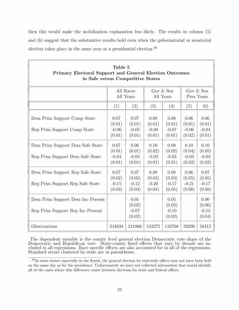
then this would make the mobilization explanation less likely. The results in column (5)

and (6) suggest that the substantive results hold even when the gubernatorial or senatorial

election takes place in the same year as a presidential election.30

Table 5Primary Electoral Support and General Election Outcomes

in Safe versus Competitive States

All Races Gov & Sen Gov & SenAll Years All Years Pres Years

(1) (2) (3) (4) (5) (6)

Dem Prim Support Comp State 0.07 0.07 0.08 0.08 0.06 0.06(0.01) (0.01) (0.01) (0.01) (0.01) (0.01)

Rep Prim Support Comp State -0.06 -0.05 -0.08 -0.07 -0.06 -0.04(0.01) (0.01) (0.01) (0.01) (0.02) (0.01)

Dem Prim Support Dem Safe State 0.07 0.06 0.10 0.08 0.10 0.10(0.01) (0.01) (0.02) (0.02) (0.04) (0.05)

Rep Prim Support Dem Safe State -0.04 -0.04 -0.03 -0.03 -0.03 -0.03(0.01) (0.01) (0.01) (0.01) (0.02) (0.02)

Dem Prim Support Rep Safe State 0.07 0.07 0.08 0.08 0.06 0.07(0.02) (0.02) (0.03) (0.03) (0.05) (0.05)

Rep Prim Support Rep Safe State -0.15 -0.12 -0.20 -0.17 -0.21 -0.17(0.03) (0.03) (0.04) (0.05) (0.08) (0.08)

Dem Prim Support Dem Inc Present 0.05 0.05 0.00(0.02) (0.03) (0.06)

Rep Prim Support Rep Inc Present -0.07 -0.10 -0.12(0.02) (0.02) (0.04)

Observations 244634 241866 133375 133708 59290 58415

The dependent variable is the county level general election Democratic vote share of theDemocratic and Republican vote. State-county fixed effects that vary by decade are in-cluded in all regressions. Race specific effects are also accounted for in all of the regressions.Standard errors clustered by state are in parentheses.

30In some states, especially in the South, the general election for statewide offices may not have been heldon the same day as for the presidency. Unfortunately we have not collected information that would identifyall of the cases where this difference exists between elections for state and federal offices.

31

Another alternative interpretation of the stronger relationship between primary and gen-

eral election votes for dominant parties in safe states is that this reflects the presence of

intra-party factions within the dominant party. These factional divisions may be salient in

general elections irrespective of whether the primary is contested. More generally we can-

not rule out the possibility that candidates for the dominant party in safe states have some

attribute, such as a factional affiliation, that is salient in the general election and may be

widely known even in the absence of a primary election campaign. The role of intra-party

factions in primary and general elections is an area for future research.

5. Primary Election Spill-Over Effects

In this section we investigate whether the salience of candidate attributes for one office

have spill-over effects on the elections for other offices. More specifically we examine whether

the areas where Democratic (Republican) gubernatorial and senatorial nominees do well in

the primaries are also areas where the Democratic (Republican) down-ballot candidates do

well in the general elections. We might suspect that the top-of-the-ticket nominees may

mobilize voters in particular areas to turnout and once they do they may continue to vote

for down-ballot candidates with the same partisan affiliations. We also examine whether

the reverse relationship exists – i.e. areas where the down-ballot candidate does well in the

primaries are also the areas where the top-of-the-ticket candidates do well in the general

elections.

The basic specification is the same as in equation 2 above except now the dependent

variable is the Democratic vote share for a particular down-ballot office and the independent

variables are the vote shares of the Democratic and Republican nominees for top-of-the-ticket

offices.

V DBij = αi + γj + θ1P

DDBij + θ2P

DTTij + θ3P

RDBij + θ4P

RTTij + εij (7)

If the effect of the top of the ticket candidates attributes spill over to down-ballot elections,

then we would expect θ2 > 0 and θ4 < 0. In this case we define PDTTij as the higher of the

gubernatorial or senatorial candidates’ vote share in the primary in county i of race j.

32

Table 6Spill-Overs Across Offices

Down-ballot Top-of-Ticket

All Pre- Post- All Pre- Post-1960 1960 1960 1960

Dem Nominee Primary Support 0.03 0.02 0.07 0.09 0.07 0.12(0.01) (0.005) (0.02) (0.01) (0.01) (0.02)

Down-ballot Primary Support -0.01 -0.01 -0.01(0.01) (0.01) (0.01)

Top of Ticket Primary Support 0.02 0.03 0.00(0.01) (0.01) (0.02)

Rep Nominee Primary Support -0.03 -0.03 -0.04 -0.09 -0.08 -0.10(0.01) (0.01) (0.01) (0.02) (0.02) (0.01)

Down-ballot Primary Support -0.01 0.00 -0.01(0.01) (0.02) (0.01)

Top of Ticket Primary Support -0.02 -0.03 0.00(0.01) (0.01) (0.01)

Observations 107386 64353 43033 59288 34276 25012

In the first three columns the dependent variable is the county level general election Demo-cratic vote share of the Democratic and Republican vote for down-ballot offices. In columns(4)-(6), the dependent variable is the county level general election Democratic vote share ofthe Democratic and Republican vote for top of the ticket offices. State-county fixed effectsthat vary by decade are included in all regressions. Race specific effects are also accountedfor in all of the regressions. Standard errors clustered by state are in parentheses.

We can also examine the less likely reverse spill-over effect, where the dependent vari-

able is the Democratic vote share for top-of-the-ticket offices and the independent variables

include the primary vote shares of nominee’s for down-ballot offices. As above we use the

highest vote share among the down-ballot offices in county i of race j.

V TTij = αi + γj + γ1P

DTTij + γ2P

DDBij + γ3P

RTTij + γ4P

RDBij + εij (8)

If the effect of down-ballot candidate’s attributes spill over to top-of-the-ticket elections,

then we would expect to find γ2 > 0 and γ4 < 0.

Column 1 of Table 6 includes all down-ballot races. The estimate of the coefficient on

the Top-of-the-Ticket Primary Support variable is consistent with the argument that the

personal support for top-of-the-ticket candidates spill over to down-ballot general election

33

outcomes. Although substantively, the coefficient estimates are relatively small when down-

ballot general election outcome is the dependent variable, the coefficient estimate on top-

of-the-ticket support is about two-thirds the size of the coefficient on down-ballot primary

support. The results in column 2 examine down-ballot general elections in the pre-1960

period and the results in column 3 examine the post-1960 period. These results suggest

that the spill over effects from the top-of-the-ticket primaries to the down-ballot general

elections are mainly in the earlier period. There is little evidence that the spill over effect

from down-ballot to top-of-the-ticket races is present in the post-1960 period.

The next three columns of Table 6 examine the spill over effects from the personal vote

for down-ballot offices on the top-of-the-ticket races. When the dependent variable is top-

of-the-ticket general election outcomes, the coefficents on the Down-ballot Primary Support

variable is small in magnitude and not statistically significant. This result suggest that

there is little reverse spillover of the personal attributes of down-ballot candidates on the

top-of the ticket general elections. This result is not very surprising since, as we mentioned

above, down-ballot candidates are often given less media attention and have access to fewer

campaign resources.

6. Conclusions

The results above indicate that there are significant linkages between primary and gen-

eral elections. First, although scholars often discuss the rise of candidate-centered politics in

the 1960s, our state level analyses indicate that there was a rise in split-ticket voting much

earlier in the century, particularly in states that introduced mandatory direct primaries be-

tween 1900 and 1915. Second, our county level analyses suggest that candidate attributes

salient in the primaries are also salient in the general elections, and this was true even in

the decades prior to the 1960s. Third, and perhaps most interestingly, we find evidence

that primary competition affects the salience of particular candidate attributes in the gen-

eral elections. While the causal effect of primaries on general election voting is perhaps

the most difficult to establish, the analyses of runoff elections and safe versus competitive

states provide some suggestive evidence that primary competition may affect the salience

34

of the candidate attributes raised during the primary campaigns in the general elections.

In addition, voters’ preferences for top-of-the-ticket candidates appear to affect voting for

down-ballot candidates, at least in the early part of the 20th century. Thus primary election

competition for high level offices may have a wider impact on politics outside the specific

office being contested.

The findings above establish a clear association, but do not identify the specific mech-

anisms. Is the relationship between candidate attributes in primary and general elections

reflecting voter information about the candidates positions? Alternatively, does it merely

reflect some type of psychological attachment to the candidates as suggested in the divisive

primaries literature? If the former is true, then our results suggest that primary competition

may play a significant role in informing the electorate about candidate attributes aside from

what can be learned from their partisan affiliations.

Using information about candidates’ issue positions, which are collected from newspaper

reports and interest group endorsements, we find some preliminary evidence that candidates’

issue positions affect their primary election votes. In a related paper we use survey data from

primary elections to show that primary voters can learn about the ideological positions of the

candidates over the course of the primary campaign (Hirano et. al. 2012). Such evidence,

along with the results in this paper, suggests that primaries may have an important role in

informing the electorate.

Our findings may understate the overall effect of primary competition, especially if can-

didates can adapt their positions, and also their campaign strategies, in response to issues

raised by their general election opponents, or their opponents’ attributes. If so, then primary

competition might have broader effects on politics and policy outcomes. For example, does

competition in primaries lead campaigns, even in the general election, to raise new issues?

Does primary competition raise the salience of particular candidate attributes, which would

have otherwise been ignored? Does primary competition even effect policy agendas and

outcomes? Further theoretical and empirical research is clearly necessary to assess the true

impact of primary elections.

35

References

Aldrich, John H. 1995. Why Parties? The Origin and Transformation of Political Partiesin America. Chicago: The University of Chicago Press.

Aldrich, John H. and Richard G. Niemi. 1990. “The Sixth American Party System: The1960s Realignment and the Candidate-Centered Parties.” Unpublished manuscript.Duke University Program in Political Economy.

Alford, John R. and David W. Brady. 1989. “Personal and Partisan Advantage in U.S.Congressional Elections, 1846-1986.” In Congress reconsidered ed. Lawrence C. Doddand Bruce I. Oppenheimer. 4th ed. Washington, D.C.: CQ Press.

Ansolabehere, Stephen and James M. Snyder. 2002. “The Incumbency Advantage in U.S.Elections: An Analysis of State and Federal Offices, 1942-2000.” Election Law Journal:Rules, Politics, and Policy. 1(3): 315-338.

Ansolabehere, Stephen, J. Mark Hansen, Shigeo Hirano and James M. Snyder. 2006. “TheDecline of Competition in U.S. Primary Elections, 1908-2004” in The Marketplace ofDemocracy, Michael McDonald and John Samples (eds.), Brookings Institution Press,Ch. 4, pages 74-101.

Ansolabehere, Stephen, Shigeo Hirano and James M. Snyder. 2007. “What Did the DirectPrimary Do to Party Loyalty in Congress?”, in Process, Party and Policy Making:Further New Perspectives on the History of Congress, Volume 2, David Brady andMathew D. McCubbins (eds.), Stanford University Press, Ch. 2, pages 21-36.

Ansolabehere, Stephen, J. Mark Hansen, Shigeo Hirano and James M. Snyder. 2010.“More Democracy: The Direct Primary and Competition in U.S. Elections.” Studiesin American Political Development. 24:190-205.

Born, R. 1981. “The Influence of House Primary Election Divisiveness on General ElectionMargins, 1962-1976.” The Journal of Politics. 42:640-61.

Bouton, Laurent. 2010. “A Theory of Strategic Voting in Runoff Elections.” Unpublishedmanuscript. Boston University.

Bullock, Charles S. III and Loch K. Johnson. 1992. Runoff Elections in the United States.Chapel Hill: The University of North Carolina Press.

Burnham, Walter Dean. 1965. “The Changing Shape of the American Political Universe.”The American Political Science Review. 59:1:7-28.

Campbell, Andrea L. 2007. “Parties, Electoral Participation, and Shifting Voting Blocs.”In The Transformation of American Politics: Activist Government and the Rise ofConservatism, edited by Paul Pierson and Theda Skocpol. Princeton, NJ: PrincetonUniversity Press.

36

Campbell, Angus and Warren Miller. 1957. “The Motivational Basis of Straight and SplitTicket Voting.” The American Political Science Review. 51:2:293-312.

Campbell, Angus, Philip E. Converse, Warren E. Miller and Donald E. Stokes. 1957. TheAmerican Voter. Chicago: University of Chicago Press.

Carey, John M. and Matthew S. Shugart. 1993. “Incentives to Cultivate a Personal Vote:a Rank Ordering of Electoral Formulas.” Electoral Studies. 14: 417-439.

Carson, Jamie L., Erik J. Engstrom and Jason M. Roberts. 2007. “Candidate Quality, thePersonal Vote, and the Incumbency Advantage in Congress.” The American PoliticalScience Review. 101:2:289-301.

Gerber, Elizabeth and Rebecca Morton. 1998. “Primary Election Systems and Represen-tation.” Journal of Law, Economics, and Organization. 14:304-24;

Hacker, A. 1965. “Does a Divisive Primary Harm a Candidate’s Election Changes?” Amer-ican Political Science Review. 59: 105-110.

Harvey, Anna and Bumba Mukherjee. n.d. “The Evolution of Partisan Conventions, 1880-1940.” Typescript.

Herrnson, Paul S. 1988. Party campaigning in the 1980s. Cambridge: Harvard UniversityPress.

Hirano, Shigeo, Maksim L. Pinkovskiy, and James M. Snyder Jr. 2012. “Voter Learningin State Primary Elections.” Typescript

Jewell, Malcolm E. 1977. “Voting Turnout in State Gubernatorial Primaries.” VotingTurnout in State Gubernatorial Primaries. 30:2:236-254.

Jacobson, Gary C. 2004. The Politics of Congressional Elections. 6th ed. New York:Harper Collins.

Kanthak, Kristin and Rebecca Morton. 2001. “The Effects of Electoral Rules on Con-gressional Primaries.” in Congressional Primaries and the Politics of Representation.Peter F. Galderisi, Marni Ezra, and Michael Lyons (eds.), Maryland: Rowman &Littlefield Publishers.

Kenney, Patrick J. and T.W. Rice. 1984. “The Effect of Primary Divisiveness in Guber-natorial and Senatorial Elections.” The Journal of Politics. 46:904-915.

Kenney, Patrick J. 1988. “Sorting Out the Effects of Primary Divisiveness in Congressionaland Senatorial Elections.” Western Political Quarterly.

Key, V.O. Jr. 1949. Southern Politics in State and Nation. New York: Knopf.

Key, V.O. Jr. 1964. Politics, Parties and Pressure Groups. New York: Crowell.

Miller, Penny M., Malcolm E. Jewell and Lee Sigelman. 1988. “Divisive Primaries andParty Activists: Kentucky, 1979 and 1983.” The Journal of Politics. 50: 459-470.

37

Nie, Norman H., Sidney Verba, and John R. Petrocik. 1979. The Changing AmericanVoter. Cambridge: Harvard University Press.

Reynolds, John F. 2006. The demise of the American convention system, 1880-1911. NewYork: Cambridge University Press.

Romero, David W. 2003. “Divisive Primaries and Incumbent General Election Perfor-mance: Prospects and Costs in U.S. House Races.” American Politics Research. 38:931-55.

Rusk, Jerrold G. 1970. “The Effect of the Australian Ballot Reform on Split Ticket Voting:1876-1908.” The American Political Science Review. 64:4:1220-1238.

Shively, W. Phillips. 1992. “From Differential Abstention to Conversion: A Change inElectoral Change, 1864-1988.” American Journal of Political Science. 36:309-30.

Ware, A. 1979. “Divisive Primaries: The Important Questions.” British Journal of Polit-ical Science. 9:381-84.

Wattenberg, Martin P. 1990. The Decline of American Political Parties: 1952-1988. Cam-bridge: Harvard University Press.

Wattenberg, Martin P. 1991. The Rise of Candidate-Centered Politics: Presidential Elec-tions of the 1980s. Cambridge: Harvard University Press.

38