The Dirichlet problem for higher order equations in

composition form

Ariel Barton∗

School of Mathematics, University of Minnesota, 127 Vincent Hall, 206 Church St. SE,

Minneapolis, Minnesota 55455

Svitlana Mayboroda

School of Mathematics, University of Minnesota, 127 Vincent Hall, 206 Church St. SE,Minneapolis, Minnesota 55455

Abstract

The present paper commences the study of higher order differential equa-

tions in composition form. Specifically, we consider the equation Lu =

divB∗∇(a divA∇u) = 0, where A and B are elliptic matrices with complex-

valued bounded measurable coefficients and a is an accretive function. Ellip-

tic operators of this type naturally arise, for instance, via a pull-back of the

bilaplacian ∆2 from a Lipschitz domain to the upper half-space. More gen-

erally, this form is preserved under a Lipschitz change of variables, contrary

to the case of divergence-form fourth order differential equations. We estab-

lish well-posedness of the Dirichlet problem for the equation Lu = 0, with

boundary data in L2, and with optimal estimates in terms of nontangential

maximal functions and square functions.

Keywords: Dirichlet problem, higher order elliptic equation

∗Corresponding authorEmail addresses: abarton@math.umn.edu (Ariel Barton), svitlana@math.umn.edu

(Svitlana Mayboroda)

Preprint submitted to Journal of Functional Analysis October 26, 2012

2010 MSC: 35J40, 31B20, 35C15

1. Introduction

The last few decades have witnessed a surge of activity on boundary-

value problems on Lipschitz domains for second-order divergence-form elliptic

equations − divA∇u = 0. Their investigation has, in particular, been guided

by two principles.

First, divergence-form equations are naturally associated to a bilinear

“energy” form, and admit a variational formulation. It turns out that some

smoothness of the coefficients A in a selected direction is necessary for well-

posedness of the underlying boundary problems in Rn+1+ = (x, t) : x ∈

Rn, t > 0 (see [? ]). This observation led to the study of the coefficients

constant along a single coordinate (the t-coordinate when n ≥ 2). The well-

posedness of the corresponding boundary-value problems was established for

real symmetric matrices in [? ? ], and the real non-symmetric case was

recently treated in [? ? ? ? ]. In addition, the resolution of the Kato

problem [? ] provided well-posedness for complex t-independent matrices in

a block form; see [? ? ]. Furthermore, a number of perturbation-type results

have been obtained, pertaining to the coefficient matrices close to “good”

ones in the sense of the L∞ norm [? ? ? ? ? ], or in the sense of Carleson

measures [? ? ? ? ? ? ? ? ? ? ? ].

A seemingly different point of view emerges from the ultimate goal of

treating boundary-value problems on non-smooth domains rather than just

the upper half-space. However, it brings to focus equations of the same type

as above. Indeed, the direct pull-back of the Laplacian ∆ from a Lipschitz

2

domain (x, t) : t > ϕ(x) to Rn+1+ yields a boundary-value problem for

an operator of the form − divA∇u = 0 on Rn+1+ , and the corresponding

matrix A is, once again, independent of t. More generally, if ρ is a change

of variables, then there is a real symmetric matrix A = A(x) such that if

∆u = 0 in Ω and u = u ρ, then divA∇u = 0 in ρ−1(Ω).

The model higher order differential operator is the bilaplacian ∆2 =

−∆(−∆). Investigating the behavior of biharmonic functions under changes

of variables, we find that there exists a scalar-valued function a and a real

elliptic matrix A such that, if ∆2u = 0 in Ω, then

divA∇(a divA∇u) = 0 in ρ−1(Ω), (1)

More generally, such a form is preserved under changes of variables. We

emphasize that this is not the case for higher order operators in divergence

form (−1)m∑|β|=|γ|=m ∂

βAβγ∂γ.

In addition, the form appearing in (1) mimics the structure of the bi-

laplacian as a composition of two Laplace operators. As it turns out, this is

an important feature that underpins several key properties of the solutions

to the biharmonic and polyharmonic equations (−∆)mu = 0, m ≥ 1.

Motivated by these considerations, the present paper commences the

study of well-posedness problems for higher order equations in composition

form. Specifically, consider the equation

divB∗∇(a divA∇u) = 0. (2)

Here a : Rn+1 7→ C is a scalar-valued accretive function and A and B are

(n+ 1) × (n+ 1) elliptic matrices with complex coefficients. That is, there

3

exist constants Λ > λ > 0 such that, if M = A or M = B, then

λ ≤ Re a(X) ≤ |a(X)| ≤ Λ, λ|η|2 ≤ Re η ·M(X)η, |ξ ·M(X)η| ≤ Λ|η||ξ|

(3)

for all X ∈ Rn+1 and all vectors ξ, η ∈ Cn+1. The second-order opera-

tors divA∇ and divB∗∇ are meant in the weak sense; see Definition 15

below for a precise definition. We assume that the coefficients a, A and B

are t-independent; no additional regularity assumptions are imposed. For

technical reasons we also require that A and B satisfy the De Giorgi-Nash-

Moser condition, that is, that solutions u to divM∇u = 0 are locally Holder

continuous for M = A, B, A∗ and B∗.

The main result of this paper is as follows. We show that whenever

the second order regularity boundary-value problems for A and B are well-

posed, and whenever the operator L = divB∗∇ a divA∇ is close to being

self-adjoint, the L2-Dirichlet problemdivB∗∇(a divA∇u) = 0 in Rn+1

+ ,

u = f on ∂Rn+1+ , ∇f ∈ L2(Rn),

~en+1 · A∇u = g on ∂Rn+1+ , g ∈ L2(Rn),

(4)

has a unique solution u that satisfies the optimal estimates

N+(∇u) ∈ L2(Rn) and 9t divA∇u9+ <∞,

where

N+(∇u)(x) = sup

( B((y,s),s/2)

|∇u|2)1/2

: y ∈ Rn, |x− y| < s

and where

9t F9+ =

ˆRn

ˆ ∞0

|F (x, t)|2 t dt dx.

4

Specifically, we will construct solutions whenever ‖Im a‖L∞(Rn) and ‖A−B‖L∞(Rn)

are sufficiently small. It is assumed that the second-order regularity problem

divA∇u = 0 in Rn+1± , u = f on ∂Rn+1

± , N±(∇u) ∈ L2(Rn)

has a unique solution in both the upper and lower half-spaces whenever

∇f ∈ L2(Rn), and that the same is true for A∗. By perturbation results in

[? ], an analogous statement is then automatically valid for B and B∗.

We will construct solutions using layer potentials; the De Giorgi-Nash-

Moser requirement mentioned above is necessary for this approach and at the

moment is common in the theory of second-order problems. If, for example,

A and B are real symmetric or complex and constant, then the De Giorgi-

Nash-Moser condition is valid and regularity problems are well-posed; hence,

in these cases there is well-posedness of (4). We mention that in passing we

prove that if the second-order regularity problems are well-posed then the

solutions necessarily can be written as layer potentials.1 This fact is new

and interesting on its own right. We will precisely state the main theorems

in Section 2.2, after the notation of this paper has been established.

Let us point out that to the best of the authors’ knowledge, this is the

first result regarding well-posedness of higher order boundary-value problems

with non-smooth variable coefficients and with boundary data in Lp. For

divergence form equations, some results for boundary data in Besov and

1This result is tantamount to proving invertibility of the single layer potential. The

method of establishing injectivity from the regularity problem and from jump relations is

known; the authors would like to thank Carlos Kenig for bringing this argument to their

attention. The method of establishing surjectivity is new and again uses jump relations.

5

Sobolev spaces Lpα, 0 < α < 1, are available (see [? ? ]), but they do not

reach out to the “end-point” case of Lp data. Until now, well-posedness

in Lipschitz domains with Lp data was known only for constant coefficient

higher order operators (see [? ? ? ? ? ? ? ]). As explained above, our

results extend to Lipschitz domains automatically via a change of variables.

(See Theorem 40 for the precise statement.)

Let us discuss the history of the subject and our methods in more detail.

We will concentrate on higher order operators and only mention the second

order results that directly affect our methods. The basic boundary-value

problem for elliptic differential equations of order greater than 2 is the Lp-

Dirichlet problem for the biharmonic operator ∆2. It is said to be well-posed

in a domain Ω if, for every f ∈ W p1 (∂Ω) and g ∈ Lp(∂Ω), there exists a

unique function u that satisfies

∆2u = 0 in Ω, u = f on ∂Ω, ν · ∇u = g on ∂Ω, NΩ(∇u) ∈ Lp(∂Ω)

(5)

where ν is the outward unit normal derivative and

NΩ(∇u)(X) = sup|∇u(Y )| : Y ∈ Ω, |X − Y | < (1 + a) dist(Y, ∂Ω) (6)

for some constant a > 0. In [? ? ? ], well-posedness of the Lp-Dirichlet

problem for ∆2 was established in C1 domains for any 1 < p < ∞. (This

result is also valid in convex domains; see [? ? ].) For general Lipschitz

domains, the L2-Dirichlet problem for ∆2 was shown to be well-posed by

Dahlberg, Kenig and Verchota in [? ] (when the domain is bounded; cf. [? ,

Theorem 3.7] for domains above Lipschitz graphs).

The sharp range of p for which the Lp-Dirichlet problem is well-posed in

6

n-dimensional Lipschitz domains is a difficult problem, still open in higher

dimensions even for the bilaplacian (cf. [? ? ]). We do not tackle the

well-posedness in Lp, p 6= 2, in the present paper; it is a subject for future

investigation. However, let us mention in passing that for the bilaplacian the

sharp results are only known in dimensions less than or equal to 7 [? ? ? ]

and, in a dramatic contrast with the case of the second order boundary-value

problems, there is a sharp dimension-dependent upper bound on the range

of well-posedness. That is, if Ω ⊂ Rn is a Lipschitz domain, then solutions

to (5) are guaranteed to exist only for 2 ≤ p ≤ pn for some pn <∞. Related

counterexamples can be found in [? , Theorem 10.7]. See also [? ] for a

review of this and related matters.

Our methods in the present paper depart from the ideas in [? ] and [? ].

The solution is represented via

u(X) = −DAf(X)− SAg(X) + EB,a,Ah(X).

Here DA and SA are the classic double and single layer potentials associated

to the operator divA∇, given by the formulas

DAf(x, t) = −ˆRn

~en+1 · A∗(y)∇ΓA∗

(x,t)(y, 0) f(y) dy,

SAg(x, t) =

ˆRn

ΓA∗

(x,t)(y, 0) g(y) dy

where ΓA∗

X is the fundamental solution to − divA∗∇ (that is, the solution

to − divA∗∇ΓA∗

X = δX). On the other hand, EB,a,A is a new layer potential,

specifically built for the problem at hand, to satisfy

−a divA∇EB,a,Ah = 1Rn+1+∂2n+1SB∗h.

7

See Section 2.4. This resembles the formula used in [? ] to construct solu-

tions to ∆2u = 0. To prove existence of solutions to (4) or (5), in addition

to the second order results, we require appropriate nontangential maximal

function (and square-function) estimates for the new potential EB,a,A, as well

as the invertibility of h 7→ ∂n+1EB,a,Ah|∂Rn+1+

in L2. However, beyond the

representation formula and invertibility argument, our method is necessarily

different from [? ] and [? ].

After a certain integration by parts, the bounds on the nontangential max-

imal function of the new potential Eh in the case of the bilaplacian become

an automatic consequence of the Calderon-Zygmund theory and boundedness

of the Cauchy integral in L2. On the other hand, for a general composition

operator, the related singular integral operators do not fall under the scope

of the Calderon-Zygmund theory and, because of the presence of non-smooth

matrices A and B, are not amenable to a similar integration by parts. We

develop an alternative argument, appealing to some elements of the method

in [? ], to obtain square function bounds, and then employ the jump relations

and intricate interplay between solutions in the upper and lower half-spaces

to obtain the desired nontangential maximal function estimates.

It is interesting to observe that, given an involved composition form of the

operator, with several “layers” of non-smooth coefficients, the difficulties also

manifest themselves in the absence of a classical variational formulation. In

particular, such standard properties of solutions as the Caccioppoli inequality

have to be reproven and even the existence of the Green function or funda-

mental solution in Rn+1 is not obvious, in any function space. In the same

vein, the existence of the normal derivative of a solution cannot be viewed as

8

the result of an integration by parts and an approximation scheme. Instead,

it once again calls for some special properties of the associated higher order

potentials.

Needless to say, our results build extensively on the developments from

the theory of second-order divergence form operators LA = − divA∇. We

refer the reader to [? ] for a detailed summary of the theory as it stood in

the mid-1990s, and to the papers [? ? ? ? ? ? ? ? ? ? ? ? ? ? ] for more

recent developments.

Finally, let us mention that aside from the the Dirichlet case, it is natural

to consider the Neumann and regularity problems as well as the inhomoge-

neous equation Lu = f , for f in a suitable function space. Recent achieve-

ments in this direction for higher order equations include [? ? ? ], [? ? ?

], and [? ? ? ? ] respectively. Unfortunately, much as in the homogeneous

Dirichlet case, they concentrate mostly on constant coefficients, with the ex-

ception of [? ? ]; these two papers consider the inhomogeneous problem

Lu = f but require that the boundary data have extra smoothness in Lp.

The outline of this paper is as follows. In Section 2 we will define the

notation used throughout this paper and state our main results. In Section 3

we will review known results from the theory of second-order operators of the

form LA = − divA∇. In Section 4, we will prove fourth-order analogues to

some basic theorems concerning solutions to second-order equations, such as

the Caccioppoli inequality. We will construct solutions to (4) using potential

operators and establish that these potentials are well-defined and bounded in

Sections 5, 6 and 7. The invertibility and uniqueness results will be presented

in Section 8 together with the end of proof of the main theorems.

9

2. Notation and the main theorems

In this section we define the notation used throughout this paper; in

Section 2.2 we will state our main theorems. (The proofs will be delayed

until Section 8.)

We work in the upper half-space Rn+1+ = Rn × (0,∞) and the lower half-

space Rn+1− = Rn × (−∞, 0). We identify ∂Rn+1

± with Rn. The coordinate

vector ~e = ~en+1 is the inward unit normal to Rn+1+ and the outward unit

normal to Rn+1− . We will reserve the letter t to denote the (n+1)st coordinate

in Rn+1.

If Ω is an open set (contained in Rn or Rn+1), then W 21 (Ω) denotes the

Sobolev space of functions f ∈ L2(Ω) whose weak gradient ∇f also lies in

L2(Ω), and W 2−1(Ω) denotes its dual space. The local Sobolev space W 2

1,loc(Ω)

denotes the set of all functions f that lie in W 21 (V ) for all open sets V

compactly contained in Ω. We let W 21 (Rn) be the completion of C∞0 (Rn)

under the norm ‖f‖W 21 (Rn) = ‖∇f‖L2(Rn); equivalently W 2

1 (Rn) is the space

of functions f ∈ W 21,loc(Rn) for which ‖∇f‖L2(Rn) is finite. Observe that

functions in W 21 (Rn) are only defined up to additive constants.

If u ∈ W 21,loc(Ω) for some Ω ⊂ Rn+1, we let∇‖u denote the gradient of u in

the first n variables, that is, ∇‖u = (∂1u, ∂2u, . . . , ∂nu). We will occasionally

use ∇‖ to denote the full gradient of a function defined on Rn.

As in [? ? ] and other papers, we will let the triple-bar norm denote the

L2 norm with respect to the measure (1/|t|) dx dt. That is, we will write

9F92± =

ˆ ∞0

ˆRn

|F (x,±t)|2 dx 1

tdt, 9F92 = 9F92

+ + 9F92− (7)

with the understanding that a t inside a triple-bar norm denotes the (n+1)st

10

coordinate, that is,

9t F92± =

ˆ ∞0

ˆRn

|F (x,±t)|2 dx t dt.

We let B(X, r) denote balls in Rn+1 and let ∆(x, r) denote “surface balls”

on ∂Rn+1± , that is, balls in Rn. If Q ⊂ Rn or Q ⊂ Rn+1 is a cube, we let `(Q)

denote its side-length, and let rQ denote the concentric cube with side-length

r`(Q). If E is a set and µ is a measure, we letffl

denote the average integralfflEf dµ = 1

µ(E)

´Ef dµ.

We will use the standard nontangential maximal function N , as well as

the modified nontangential maximal function N introduced in [? ]. These

functions are defined as follows. If a > 0 is a constant and x ∈ Rn, then the

nontangential cone γ±(x) is given by

γ±(x) =

(y, s) ∈ Rn+1± : |x− y| < a|s|

. (8)

The nontangential maximal function and modified nontangential maximal

function are given by

N±F (x) = sup |F (y, s)| : (y, s) ∈ γ±(x) , (9)

N±F (x) = sup

( B((y,s),|s|/2)

|F |2)1/2

: (y, s) ∈ γ±(x)

. (10)

We remark that by [? , Section 7, Lemma 1], if we let

NaF (x) = sup |F (y, s)| : |x− y| < as, 0 < s ,

then for each 1 ≤ p ≤ ∞ and for each 0 < b < a, there is a constant C

depending only on p, a and b such that ‖NaF‖Lp(Rn) ≤ C‖NbF‖Lp(Rn). Thus,

for our purposes, the exact value of a in (8) is irrelevant provided a > 0.

11

Suppose that A : Rn+1 7→ C(n+1)×(n+1) is a bounded measurable matrix-

valued function defined on Rn+1. We let AT denote the transpose matrix and

let A∗ denote the adjoint matrix AT . Recall from the introduction that A is

elliptic if there exist constants Λ > λ > 0 such that

λ|η|2 ≤ Re η · A(X)η, |ξ · A(X)η| ≤ Λ|η||ξ| (11)

for all X ∈ Rn+1 and all vectors η, ξ ∈ Cn+1. We refer to λ and Λ as the

ellipticity constants of A. Recall also that a scalar function a is accretive if

λ ≤ Re a(X) ≤ |a(X)| ≤ Λ for all X ∈ Rn+1. (12)

We say that a function or coefficient matrix A is t-independent if

A(x, t) = A(x, s) for all x ∈ Rn and all s, t ∈ R. (13)

2.1. Elliptic equations and boundary-value problems

If A is an elliptic matrix, then for any u ∈ W 21,loc(Ω), the expression

LAu = − divA∇u ∈ W 2−1,loc(Ω) is defined by

〈ϕ,LAu〉 =

ˆΩ

ϕLAu =

ˆ∇ϕ · A∇u for all ϕ ∈ C∞0 (Ω). (14)

If A and B are elliptic matrices and a is an accretive function, we may define

L∗B(aLAu) in the weak sense as follows.

Definition 15. Suppose u ∈ W 21,loc(Ω). Then LAu = − divA∇u is a well-

defined element of W 2−1,loc(Ω). Suppose that aLAu = v, for some v ∈

W 21,loc(Ω), in the sense that

ˆ∇ϕ · A∇u =

ˆϕ

1

av for all ϕ ∈ C∞0 (Ω).

12

If v satisfies

ˆ∇v ·B∇η =

ˆηf for all η ∈ C∞0 (Ω),

that is, if− divB∗∇v = f in the weak sense, then we say that L∗B(aLAu) = f .

Suppose that U is defined in Rn+1± . We define the boundary values of U

as as the L2 limit of U up to the boundary, that is,

U∣∣∂Rn+1±

= F provided limt→0±‖U( · , t)− F‖L2(Rn) = 0. (16)

Given these definitions, we may define the Dirichlet problem for the

fourth-order operator L∗B(aLA) as follows.

Definition 17. Suppose that there is a constant C0 such that, for any f ∈

W 21 (Rn) and any g ∈ L2(Rn), there exists a unique function u ∈ W 2

1,loc(Rn+1+ )

that satisfies

L∗B(aLAu) = 0 in Rn+1+ ,

u = f, ∇‖u = ∇f on ∂Rn+1+ ,

~e · A∇u = g on ∂Rn+1+ ,

‖N+(∇u)‖L2(Rn) + 9t LAu9+ ≤ C0‖∇f‖L2(Rn) + C0‖g‖L2(Rn)

(18)

where L∗B(aLAu) = 0 in the sense of Definition 15 and where the boundary

values are in the sense of (16).

Then we say that the L2-Dirichlet problem for L∗B(aLA) is well-posed

in Rn+1+ .

We specify ∇‖u = ∇f as well as u = f in order to emphasize that

u( · , t)→ f in W 21 (Rn) and not merely in L2(Rn).

13

Remark 19. The solutions u to (18) constructed in the present paper will

also satisfy the square-function estimate

9t∇∂tu9+ ≤ C1‖∇f‖2L2(Rn) + C1‖g‖2

L2(Rn) (20)

for some constant C1. If u is a solution to a fourth-order elliptic equation

with constant coefficients, then by [? ] we have a square function bound

on the complete Hessian matrix ∇2u. However, in the case of solutions to

variable-coefficient operators in the composition form of Definition 15, we do

not expect all second derivatives to be well-behaved, and so (20) cannot be

strengthened.

Our main theorem is that, if a, A and B satisfy certain requirements,

then the fourth-order Dirichlet problem (18) is well-posed. We now define

these requirements. We begin with the De Giorgi-Nash-Moser condition.

Definition 21. We say that a function u is locally Holder continuous in

the domain Ω if there exist constants H and α > 0 such that, whenever

B(X0, 2r) ⊂ Ω, we have that

|u(X)− u(X ′)| ≤ H

(|X −X ′|

r

)α( B(X0,2r)

|u|2)1/2

(22)

for all X, X ′ ∈ B(X0, r). If u is locally Holder continuous in B(X, r) for

some r > 0, then u also satisfies Moser’s “local boundedness” estimate

|u(X)| ≤ C

( B(X,r)

|u|2)1/2

(23)

for some constant C depending only on H and the dimension n+ 1.

If A is a matrix, we say that A satisfies the De Giorgi-Nash-Moser condi-

tion if A is elliptic and, for every open set Ω and every function u such that

14

divA∇u = 0 in Ω, we have that u is locally Holder continuous in Ω, with

constants H and α depending only on A (not on u or Ω).

Throughout we reserve the letter α for the exponent in the estimate (22).

We will show (see Corollary 77 below) that if A, A∗ and B∗ satisfy the De

Giorgi-Nash-Moser condition then solutions to L∗B(aLAu) = 0 are also locally

Holder continuous.

We say that the L2-regularity problem (R)A2 is well-posed in Rn+1± if, for

each f ∈ W 21 (Rn), there is a function u, unique up to additive constants,

that satisfies

(R)A2

divA∇u = 0 in Rn+1

± ,

u = f on ∂Rn+1± ,

‖N±(∇u)‖L2(Rn) ≤ C‖∇f‖L2(Rn).

Remark 24. If N±(∇u) ∈ L2(Rn), then averages of u have a weak nontan-

gential limit at the boundary, in the sense that there is some function f such

that ( B((x,t),|t|/2)

|u(y, s)− f(x∗)|2 dy ds)1/2

≤ C|t|N±(∇u)(x∗)

for all (x, t) ∈ γ±(x∗). See the proof of [? , Theorem 3.1a]; here C is a

constant depending only on the constant a in the definition (8) of γ±. If u is

locally Holder continuous then this implies that u itself has a nontangential

limit, which by the dominated convergence theorem must equal its limit in

the sense of (16). Thus, the requirement in (18) or (R)A2 that u = f on ∂Rn+1±

in the sense of vertical L2 limits is equivalent to the requirement that u = f

on ∂Rn+1± in the sense of pointwise nontangential limits almost everywhere.

15

2.2. The main theorems

The main theorems of this monograph are as follows.

Theorem 25. Let a : Rn+1 7→ R and A : Rn+1 7→ C(n+1)×(n+1), where

n+ 1 ≥ 3. Assume that

• a is accretive and t-independent.

• a is real-valued.

• A is elliptic and t-independent.

• A and A∗ satisfy the De Giorgi-Nash-Moser condition.

• The regularity problems (R)A2 and (R)A∗

2 are well-posed in Rn+1± .

Then the L2-Dirichlet problem for L∗A(aLA) is well-posed in Rn+1+ , and

the constants C0 and C1 in (18) and (20) depend only on the dimension

n+ 1, the ellipticity and accretivity constants λ, Λ in (11) and (12), the De

Giorgi-Nash-Moser constants H and α, and the constants C in the definition

of (R)A2 and (R)A∗

2 .

We can generalize Theorem 25 to the following perturbative version.

Theorem 26. Let A be as in Theorem 25, and let a : Rn+1 7→ C be accretive

and t-independent. Let B : Rn+1 7→ C(n+1)×(n+1) be t-independent.

There is some ε > 0, depending only on the quantities listed in Theo-

rem 25, such that if

‖Im a‖L∞(Rn) < ε and ‖A−B‖L∞(Rn) < ε,

16

then the L2-Dirichlet problem for L∗B(aLA) is well-posed in Rn+1+ , and the

constants C0 and C1 in (18) and (20) depend only on the quantities listed in

Theorem 25.

We will see that if ε is small enough then B also satisfies the conditions

of Theorem 25; see Theorem 27. It is possible to generalize from Rn+1+ to

domains above Lipschitz graphs; see Theorem 40 below.

We remark that throughout this paper, we will let C denote a positive

constant whose value may change from line to line, but which in general

depends only on the quantities listed in Theorem 25; any other dependencies

will be indicated explicitly.

In the remainder of this section we will remind the reader of some known

sufficient conditions for a matrix A to satisfy the De Giorgi-Nash-Moser

condition or for the regularity problem (R)A2 to be well-posed. To prove

Theorems 25 and 26, we will need some consequences of these conditions; we

will establish notation for these consequences in Section 2.3.

We begin with the De Giorgi-Nash-Moser condition. Suppose that A is

elliptic. It is well known that if A is constant then solutions to divA∇u = 0

are smooth (and in particular are Holder continuous). More generally, the De

Giorgi-Nash-Moser condition was proven to hold for real symmetric coeffi-

cients A by De Giorgi and Nash in [? ? ] and extended to real nonsymmetric

coefficients by Morrey in [? ]. The De Giorgi-Nash-Moser condition is also

valid if A is t-independent and the ambient dimension n + 1 = 3; this was

proven in [? , Appendix B].

Furthermore, this condition is stable under perturbation. That is, let A0

be elliptic, and suppose that A0 and A∗0 both satisfy the De Giorgi-Nash-

17

Moser condition. Then there is some constant ε > 0, depending only on the

dimension n+ 1 and the constants λ, Λ in (11) and H, α in (22), such that if

‖A− A0‖L∞(Rn+1) < ε, then A satisfies the De Giorgi-Nash-Moser condition.

This result is from [? ]; see also [? , Chapter 1, Theorems 6 and 10].

We observe that in dimension n + 1 ≥ 4, or in dimension n + 1 = 3 for

t-dependent coefficients, the De Giorgi-Nash-Moser condition may fail; see

[? ] for an example.

The regularity problem (R)A2 has been studied extensively. In particular,

if A is t-independent, then (R)A2 is known to be well-posed in Rn+1± provided

A is constant, real symmetric ([? ]), self-adjoint ([? ]), or of “block” form

A(x) =

A‖(x) ~0

~0T a⊥(x)

for some n× n matrix A‖ and some complex-valued function a⊥. The block

case follows from validity of the Kato conjecture, as explained in [? , Re-

mark 2.5.6]; see [? ] for the proof of the Kato conjecture and [? , Conse-

quence 3.8] for the case a⊥ 6≡ 1.

Furthermore, well-posedness of (R)A2 is stable under perturbation by [?

]; that is, if (R)A02 is well-posed in Rn+1

± for some elliptic t-independent

matrix A0, then so is (R)A2 for every elliptic t-independent matrix A with

‖A− A0‖L∞ small enough.

We mention that if A is a nonsymmetric matrix, the L2-regularity problem

need not be well-posed, even in the case where A is real. See the appendix

to [? ] for a counterexample.

We may summarize the results listed above as follows.

18

Theorem 27. Let A be elliptic and t-independent, and suppose that the

dimension n + 1 is at least 3. If A satisfies any of the following conditions,

then A satisfies the conditions of Theorem 25.

• A is constant.

• A is real symmetric.

• A is a 3× 3 self-adjoint matrix.

• A is a real or 3× 3 block matrix.

If A0 satisfies the conditions of Theorem 25, and if ‖A− A0‖L∞(Rn) < ε for

some ε depending only on the quantities enumerated in Theorem 25, then A

also satisfies the conditions of Theorem 25.

2.3. Second-order boundary-value problems and layer potentials

In order to prove Theorem 25, we will need well-posedness of several

second-order boundary-value problems and good behavior of layer potentials;

these conditions follow from well-posedness of (R)A2 and (R)A∗

2 .

We say that the oblique L2-Neumann problem (N⊥)A2 is well-posed in

Rn+1± if, for each g ∈ L2(Rn), there exists a unique (modulo constants) func-

tion u that satisfies

(N⊥)A2

divA∇u = 0 in Rn+1

± ,

∂n+1u = g on ∂Rn+1± ,

‖N±(∇u)‖L2(Rn) ≤ C‖g‖L2(Rn).

By [? , Proposition 2.52] and [? , Corollary 3.6] (see also [? , Proposi-

tion 4.4]), if A is t-independent, then (R)A∗

2 is well-posed in Rn+1± if and only

if (N⊥)A2 is well-posed in Rn+1± .

19

We say that the L2-Dirichlet problem (D)A2 is well-posed in Rn+1± if there

is some constant C such that, for each f ∈ L2(Rn), there is a unique function

u that satisfies

(D)A2

divA∇u = 0 in Rn+1

± ,

u = f on ∂Rn+1± ,

‖N±u‖L2(Rn) ≤ C‖f‖L2(Rn).

Observe that if u is a solution to (N⊥)A2 with boundary data f , then v =

∂n+1u is a solution to (D)A2 with boundary data f ; thus, well-posedness of

(N⊥)A2 implies existence of solutions to (D)A2 . Recall that well-posedness of

(N⊥)A2 also implies existence of solutions to (R)A∗

2 . It is possible to show

that if (R)A∗

2 solutions exist then solutions to (D)A2 are unique; see the proof

of [? , Lemma 4.31].

Thus, if (R)A∗

2 is well-posed in Rn+1± then so is (D)A2 . We observe that

this result was proven for real symmetric A by Kenig and Pipher in [? ].

The L2-Neumann problem (N)A2 more usually considered differs from

(N⊥)A2 in that the boundary condition is ~e ·A∇u = g rather than ∂n+1u = g

on ∂Rn+1+ . We remark that if A is constant, self-adjoint or of block form then

(N)A2 is known to be well-posed (again see [? ] or [? , Remark 2.5.6] and [? ?

]). (N)A2 is in many ways more natural than the oblique Neumann problem;

however, we will not use well-posedness of the traditional Neumann problem

and so do not provide a definition here.

A classic method for constructing solutions to second-order boundary-

value problems is the method of layer potentials. We will use the double and

single layer potentials of the second-order theory, as well as a new fourth-

order potential (see Section 2.4) to construct solutions to (18); thus, we will

20

need some properties of these potentials.

These potentials for second-order operators are defined as follows. The

fundamental solution to LA = − divA∇ with pole at X is a function ΓAX such

that (formally) − divA∇ΓAX = δX . For general complex coefficients A such

that A and A∗ satisfy the De Giorgi-Nash-Moser condition, the fundamental

solution was constructed by Hofmann and Kim. See [? , Theorem 3.1]

(reproduced as Theorem 52 below) for a precise definition of the fundamental

solution.

If f and g are functions defined on Rn, the classical double and single

layer potentials DAf and SAg are defined by the formulas

DAf(x, t) = −ˆRn

~e · AT (y)∇ΓAT

(x,t)(y, 0) f(y) dy, (28)

SAg(x, t) =

ˆRn

ΓAT

(x,t)(y, 0) g(y) dy. (29)

For well-behaved functions f and g, these integrals converge absolutely for

x ∈ Rn and for t 6= 0, and satisfy divA∇DAf = 0 and divA∇SAg = 0 in

Rn+1 \ Rn; see Section 3.2.

We define the boundary layer potentials

D±Af = DAf∣∣∂Rn+1±, (∇SA)±g = ∇SAg

∣∣∂Rn+1±,

S±Ag = SAg∣∣∂Rn+1±, S⊥,±A g = ∂n+1SAg

∣∣∂Rn+1±

where the boundary values are in the sense of (16).

We remind the reader of the classic method of layer potentials for con-

structing solutions to boundary-value problems. Suppose the nontangential

estimate ‖N±(∇SAg)‖L2(Rn) ≤ C‖g‖L2(Rn) is valid. Then if S±A is invert-

ible L2(Rn) 7→ W 21 (Rn), then u = SA((S±A )−1g) is a solution to (R)A2 with

21

boundary data g. Similarly, if S⊥,±A or the operator g 7→ ~e · A(∇SA)±g is

invertible on L2(Rn), then we may construct solutions to (N⊥)A2 or (N)A2 ,

respectively. The adjoint to g 7→ ~e · A(∇SA)±g is the operator D∓A∗ , and so

if we can construct solutions to (N)A2 using the single layer potential then

we can construct solutions to (D)A∗

2 using the double layer potential. In the

case of t-independent matrices, we may also construct solutions to (D)A2 by

using invertibility of S⊥,±A .

Thus, if layer potentials are bounded and invertible, we have well-posedness

of boundary-value problems. The formulas (28) and (29) for solutions are

often useful; thus, the layer potential results above are of interest even if

well-posedness is known by other methods. It turns out that we can derive

the layer potential results from well-posedness.

Lemma 30. Suppose (R)A2 and (R)A∗

2 are well-posed in Rn+1± . Then there

exists a constant C such that

9t ∂2t SAg92 =

ˆRn+1

|∂2t SAg(x, t)|2 |t| dx dt ≤ C‖g‖2

L2(Rn). (31)

Proof. Recall that if (R)A2 is well-posed then so is (D)A∗

2 . The square-function

estimate (31) follows from well-posedness of (D)A∗

2 and (R)A∗

2 via a local

T (b) theorem for square functions. This argument was carried out in [? ,

Section 8] in the case where A is real and symmetric; we refer the reader to

[? , Section 5.3] for appropriate functions b to use in the general case. (The

interested reader should note that [? , Chapter 5] is devoted to a proof of

(31) in the case of elliptic systems.)

It was observed in [? , Proposition 1.19] that by results from [? ] and [?

22

], if (31) is valid then

‖N±(∇SAg)‖L2(Rn) ≤ C‖g‖L2(Rn). (32)

Using classic techniques involving jump relations, we will show (see Theo-

rem 67 below) that if (R)A2 is well-posed in Rn+1± then S±A is invertible

L2(Rn) 7→ W 21 (Rn), and if in addition (N⊥)A2 is well-posed then S⊥,±A is

invertible. Thus, if (R)A2 and (R)A∗

2 are well-posed, then not only do so-

lutions to (R)A2 , (N⊥)A2 and (D)A2 exist, they are given by the formulas

u = SA((S±A )−1g), u = SA((S⊥,±A )−1g) and u = ∂n+1SA((S⊥,±A )−1g), respec-

tively.

In many of the results in the later parts of this paper, we will only need

a few specific consequences of well-posedness of (R)A2 and (R)A∗

2 . These

consequences are as follows.

Definition 33. Suppose that A and A∗ are elliptic, t-independent and satisfy

the De Giorgi-Nash-Moser condition.

Suppose that

• the square-function estimate (31) is valid,

• the operators S⊥,±A are invertible L2(Rn) 7→ L2(Rn), and

• solutions to the Dirichlet problem (D)A2 are unique in Rn+1+ and in Rn+1

− .

Then we say that A satisfies the single layer potential requirements.

We remark that if A satisfies the single layer potential requirements then

(N⊥)A2 (and hence (R)A∗

2 and (D)A2 ) are well-posed, and so both A and A∗

satisfy the single layer potential requirements if and only if A satisfies the

23

conditions of Theorem 25. We will prove a few bounds under the assumption

that A (not necessarily A∗) satisfies the single layer potential requirements.

We also remark that because we have no need of well-posedness of the Neu-

mann problem (N)A2 , we have not required invertibility of D±A or its adjoint.

Consequently, our layer potential requirements are weaker than those con-

sidered elsewhere in the literature.

2.4. Layer potentials for fourth-order differential equations

We will construct solutions to the fourth-order Dirichlet problem (18) us-

ing potential operators. For u = EB,a,Ah to be a solution to L∗B(aLA(Eh)) =

0, we must have that v = aLAEB,a,Ah is a solution to LB∗v = 0 in Rn+1+ .

We choose v = ∂2n+1SB∗h; if B∗ is t-independent then L∗B(∂2

n+1SB∗h) =

∂2n+1L

∗B(SB∗h) = 0. It will be seen that with this choice of v, the opera-

tor EB,a,A is bounded and invertible in some sense.

Formally, the solution to the equation

−a divA∇EB,a,Ah = 1Rn+1+∂2n+1SB∗h

is given by

EB,a,Ah(x, t) =

ˆRn

ˆ ∞0

ΓA(y,s)(x, t)1

a(y)∂2sSB∗h(y, s) ds dy.

However, to avoid certain convergence issues, we will instead define

EB,a,Ah(x, t) = FB,a,Ah(x, t)− SA(

1

aS⊥,+B∗ h

)(x, t) (34)

where the auxiliary potential FB,a,A is given by

FB,a,Ah(x, t) = −ˆRn

ˆ ∞0

∂sΓA(y,s)(x, t)

1

a(y)∂sSB∗h(y, s) ds dy. (35)

24

That these two definitions are formally equivalent may be seen by integrating

by parts in s.

In Section 5, we will show that the integral in (35) converges absolutely

for sufficiently well-behaved functions h; we will see that if A and B∗ satisfy

the single layer potential requirements, then by the second-order theory the

difference EB,a,Ah − FB,a,Ah = −SA((1/a)S⊥,+B∗ h

)is also well-defined and

satisfies square-function and nontangential bounds.

2.5. Lipschitz domains

As we discussed in the introduction, by applying the change of variables

(x, t) 7→ (x, t−ϕ(x)), boundary-value problems for the second-order operator

divA∇ in the domain Ω given by

Ω = (x, t) : x ∈ Rn, t > ϕ(x) (36)

may be transformed to boundary-value problems in the upper half-space

for an appropriate second-order operator div A∇. In particular, the theory

of harmonic functions in domains of the form (36) is encompassed by the

theory of solutions to div A∇u = 0, for elliptic t-independent matrices A, in

the upper half-space.

We now investigate the behavior of fourth-order operators under this (or

another) change of variables. Let ρ : Ω 7→ Rn+1+ be any bilipschitz change of

variables and let Jρ be the Jacobean matrix, so ∇(u ρ) = JTρ (∇u) ρ. For

any accretive function a and elliptic matrix M , we let a and M be such that

a =a ρ|Jρ|

, JρM JTρ = |Jρ| (M ρ). (37)

25

By the weak definition (14) of LM = − div M∇ and elementary multivariable

calculus, we have that if Rn+1+ is a domain, and if u ∈ W 2

1,loc(Rn+1+ ) and

LM u ∈ L2loc(R

n+1+ ), then

LM(u ρ) = |Jρ| (LM u) ρ in Ω = ρ−1(Rn+1+ ). (38)

Observe that u is Holder continuous if and only if u is; thus M satisfies the

De Giorgi-Nash-Moser condition if and only if M does.

Now, suppose that L∗B

(a LAu) = 0 in Rn+1+ , where a, A, B are given by

(37). Let u = uρ. By Definition 15, v = a LAu lies in W 21,loc(R

n+1+ ). By (38),

vρ = a (LAu) ∈ W 21,loc(Ω) and LB∗(vρ) = 0. Thus a (LAu) ∈ W 2

1,loc(Ω) and

so L∗B(aLAu) is well-defined in Ω, and furthermore L∗B(aLAu) = 0. Thus,

existence of solutions in Ω follows from existence of solutions in Rn+1+ .

Similarly, if L∗B(aLAu) = 0 in Ω and u = u ρ−1 then L∗B

(a LAu) = 0 in

Rn+1+ . Thus, uniqueness of solutions in Ω follows from uniqueness of solutions

in Rn+1+ .

We remark that the preceding argument is valid with Ω and Rn+1+ replaced

by V and ρ(V ) for any domain V .

Because we wish to preserve t-independence, we consider only the change

of variables ρ(x, t) = (x, t − ϕ(x)). This change of variables allows us to

generalize Theorem 26 to domains Ω of the form (36). The argument is

straightforward; however, to state the result we must first define the fourth-

order Dirichlet and second-order regularity problems in such domains.

Let Ω be a Lipschitz domain of the form (36). Let ν denote the unit out-

ward normal to Ω and σ denote surface measure on ∂Ω. Let W 21 (∂Ω) denote

the Sobolev space of functions in L2(∂Ω) whose weak tangential derivative

also lies in L2(∂Ω); in both cases we take the norm with respect to surface

26

measure. We say that U = F on ∂Ω if F is the vertical limit of U in L2(∂Ω),

that is, if

limt→0+

ˆ∂Ω

|U(X + t~en+1)− F (X)|2 dσ(X) = 0. (39)

If f is defined on ∂Ω, we let ∇τf be the tangential gradient of f along ∂Ω.

If u is defined in Ω, then ∇‖u is the gradient of u parallel to ∂Ω; that is,

if X = X0 + t~en+1 for some X0 ∈ ∂Ω and some t > 0, then ∇‖u(X) =

∇u(X)− (ν(X0) · ∇u(X))ν(X0).

If Ω is the domain above a Lipschitz graph, we say that the L2-Dirichlet

problem for L∗B(aLA) is well-posed in Ω if there is a constant C0 such that,

for every f ∈ W 21 (∂Ω) and every g ∈ L2(∂Ω), there exists a unique function u

that satisfies

L∗B(aLAu) = 0 in Ω,

u = f, ∇‖u = ∇τf on ∂Ω,

ν · A∇u = g on ∂Ω,

‖NΩ(∇u)‖L2(∂Ω) ≤ C0‖∇τf‖L2(Rn) + C0‖g‖L2(Rn),ˆΩ

|LAu(X)|2 dist(X, ∂Ω) dX ≤ C0‖∇τf‖L2(Rn) + C0‖g‖L2(Rn).

The modified nontangential maximal function NΩ is given by

NΩ(∇u)(X) = sup

( B(Y,dist(Y,∂Ω)/2)

|∇u|2)1/2

: Y ∈ Ω, |X − Y | < (1 + a) dist(Y, ∂Ω)

.

As in Remark 24, we also have that u→ f nontangentially in the sense that

limY→X, Y ∈γ(X)

u(Y ) = f(X), γ(X) = Y ∈ Ω, |X − Y | < (1+a) dist(Y, ∂Ω).

27

We say that the L2-regularity problem (R)A2 is well-posed in Ω if for every

f ∈ W 21 (∂Ω) there is a unique function u that satisfies

(R)A2

divA∇u = 0 in Ω,

u = f on ∂Ω,

‖NΩ(∇u)‖L2(Rn) ≤ C‖∇τf‖L2(Rn)

where u = f in the sense of either (39) or in the sense of nontangential limits.

Clearly, (R)A2 is well-posed in Ω if and only if (R)A2 is well-posed in Rn+1+ .

We may now generalize Theorem 26 to Lipschitz domains.

Theorem 40. Let Ω = (x, t) : t > ϕ(x) for some Lipschitz function ϕ.

Let a : Rn+1 7→ C, and let A, B : Rn+1 7→ C(n+1)×(n+1), where n+ 1 ≥ 3.

Suppose that a, A and B are t-independent, that a is accretive, that A and

A∗ satisfy the De Giorgi-Nash-Moser condition, and that (R)A2 and (R)A∗

2 are

well-posed in Ω and in ΩC.

Then there is some ε > 0, depending only on ‖∇ϕ‖L∞(Rn) and the quan-

tities listed in Theorem 25, such that if

‖Im a‖L∞(Rn) < ε and ‖A−B‖L∞(Rn) < ε,

then the L2-Dirichlet problem for L∗B(aLA) is well-posed in Ω.

3. Preliminaries: the second-order theory

In this section, we will review some known results concerning solutions

to second-order elliptic equations of the form divA∇u = 0, and more specif-

ically, concerning solutions to second-order boundary-value problems. In

28

Sections 3.1 and 3.2, we will discuss the second-order fundamental solution

and some properties of layer potentials.

In this section we will state several results valid in Rn+1+ ; the obvious

analogues are also valid in Rn+1− .

The following two lemmas are well known.

Lemma 41 (The Caccioppoli inequality). Suppose that A is elliptic. Let

X ∈ Rn+1 and let r > 0. Suppose that divA∇u = 0 in B(X, 2r), for some

u ∈ W 21 (B(X, 2r)). Thenˆ

B(X,r)

|∇u|2 ≤ C

r2

ˆB(X,2r)\B(X,r)

|u|2

for some constant C depending only on the ellipticity constants of A and the

dimension n+ 1.

Lemma 42. [? , Theorem 2]. Let A be elliptic, and suppose that divA∇u =

0 in B(X, 2r). Then there exists a p > 2, depending only on the constants

λ, Λ in (11), such that( B(X,r)

|∇u|p)1/p

≤ C

( B(X,2r)

|∇u|2)1/2

.

These conditions may be strengthened in the case of t-independent co-

efficients. Suppose that Q ⊂ Rn is a cube. If u satisfies divA∇u = 0 in

2Q × (t − `(Q), t + `(Q)), and if A is t-independent, then by [? , Proposi-

tion 2.1], there is some p0 > 2 such that if 1 ≤ p ≤ p0, then( Q

|∇u(x, t)|p dx)1/p

≤ C

( 2Q

t+`(Q)/4

t−`(Q)/4

|∇u(x, s)|2 ds dx)1/2

. (43)

We will show that a similar formula holds for solutions to fourth-order equa-

tions in Lemma 80 below.

More generally, we have the following lemma.

29

Lemma 44. Suppose ~f ∈ L2(Rn 7→ Cn+1) is a vector-valued function, and

that divA∇u = 0 in 2Q× (t− `(Q), t+ `(Q)) for some t-independent elliptic

matrix A. Then

Q

|∇u(x, t)− ~f(x)|2 dx ≤ C

2Q

t+`(Q)/2

t−`(Q)/2

|∇u(x, s)− ~f(x)|2 ds dx. (45)

Proof. Let v(x, t) =ffl t+`(Q)/4

t−`(Q)/4u(x, s) ds. Then

Q

|∇u(x, t)− ~f(x)|2 dx ≤ 2

Q

|∇u(x, t)−∇v(x, t)|2 dx+2

Q

|∇v(x, t)− ~f(x)|2 dx.

Define D(r) = 2Q × (t − r`(Q), t + r`(Q)). If A is t-independent then

divA∇(u− v) = 0 in D(3/4). Applying (43) to u− v, we have that

Q

|∇u( · , t)−∇v( · , t)|2 ≤ C

D(1/4)

|∇u−∇v|2.

By definition of v,

Q

|∇v(x, t)− ~f(x)|2 dx =

Q

∣∣∣∣ t+`(Q)/4

t−`(Q)/4

∇u(x, s)− ~f(x) ds

∣∣∣∣2 dx.Writing∇u−∇v = (∇u− ~f)+(∇v− ~f), and again applying the definition

of v to bound ∇v(x, s)− ~f completes the proof.

We also have the following theorems from [? ]. Although we quote

these theorems for t-independent coefficients only, in fact they are valid for

t-dependent coefficients that satisfy a Carleson-measure condition.

Theorem 46. [? , Theorem 2.4(i)]. Suppose that A is t-independent and

elliptic, that divA∇u = 0 in Rn+1+ , and that u satisfies the square-function

estimate ˆ ∞0

ˆRn

|∇u(x, t)|2 t dx dt <∞.

30

Then there is a constant c and a function f ∈ L2(Rn) such that

limt→0+‖u( · , t)− f − c‖L2(Rn) = 0

and such that

‖N+(u− c)‖2L2(Rn) ≤ C

ˆ ∞0

ˆRn

|∇u(x, t)|2 t dx dt

where C depends only on the dimension n + 1 and the ellipticity constants

λ, Λ of A. If A satisfies the De Giorgi-Nash-Moser condition then we may

replace N+u by N+u.

In the t-independent setting, (45) lets us state [? , Theorem 2.3(i)] as

follows.

Theorem 47. Suppose that divA∇u = 0 in Rn+1+ and that N+(∇u) ∈

L2(Rn), where A is elliptic and t-independent. Then there exists a function

~G : Rn 7→ Cn+1 with ‖~G‖L2(Rn) ≤ C‖N+(∇u)‖L2(Rn) such that

limt→0+‖∇u( · , t)− ~G‖2

L2(Rn) = 0 = limt→∞‖∇u( · , t)‖2

L2(Rn).

By the divergence theorem, there is a standard weak formulation of the

boundary value ~e · A∇u for any solution u to divA∇u = 0 with ∇u ∈

L2(Rn+1+ ). Theorem 47 implies that if u is an appropriately bounded solution,

then the boundary value ~e · A∇u|∂Rn+1±

exists in the sense of L2 limits. By

the following result, these two formulations yield the same value.

Theorem 48 ([? , Lemma 4.3]). Suppose that A is elliptic, t-independent

and satisfies the De Giorgi-Nash-Moser condition. Suppose that divA∇u = 0

in Rn+1+ and N+(∇u) ∈ L2(Rn).

31

Then there is some function g ∈ L2(Rn) such that, if ϕ ∈ C∞0 (Rn+1),

then ˆRn+1+

∇ϕ(x, t) · A(x)∇u(x, t) dx dt =

ˆRn

ϕ(x, 0) g(x) dx.

Furthermore, −~e · A∇u( · , t)→ g as t→ 0+ in L2(Rn).

Given a function u that satisfies divA∇u = 0 in Rn+1± , we will frequently

analyze the vertical derivative ∂n+1u. In order to make statements about u,

given results concerning ∂n+1u, we will need a uniqueness result.

Lemma 49. Let A be elliptic and t-independent. Suppose that divA∇u = 0

and ∂n+1u ≡ 0 in Rn+1+ .

If there is some constant c > 0 and some t0 > 0 such that

B((x,t),t/2)

|∇u|2 ≤ ct−n (50)

for all t > t0 and all x ∈ Rn, then u is constant in Rn+1+ .

If N+(∇u) ∈ L2(Rn) then (50) is valid for all t > 0. Thus in particular,

uniqueness of solutions to (D)A2 implies uniqueness of solutions to (N⊥)A2 .

Proof. Since ∂n+1u(x, t) = 0, we have that u(x, t) = v(x) for some function

v : Rn 7→ C. By letting t→∞ in (50) we have that ∇v ∈ L2(Rn).

Choose some x ∈ Rn and some t > 0. If τ > Ct, then let Y (τ) be the

cylinder ∆(x, t)× (τ −τ/C, τ +τ/C). By Holder’s inequality and Lemma 42,

there is some p > 2 such that

ˆ∆(x,t)

|∇v|2 =C

τ

ˆY (τ)

|∇u|2 ≤ C

τ(tnτ)1−2/p

(ˆB((x,τ),τ/C)

|∇u|p)2/p

≤ Ctn(p−2)/pτ−n(p−2)/pτn B((x,τ),2τ/C)

|∇u|2.

32

But if τ is large enough, then τnfflB((x,τ),2τ/C)

|∇u|2 ≤ c. By letting τ → ∞,

we see that ∇v ≡ 0 and so u(x, t) = v(x) is a constant.

We will also need the following uniqueness result.

Lemma 51. Let A be elliptic, t-independent and satisfy the De Giorgi-Nash-

Moser condition. Suppose that u+ and u− are two functions that satisfy

divA∇u± = 0 in Rn+1± , N±(∇u±) ∈ L2(Rn), ∇u+|∂Rn+1

+= ∇u−|∂Rn+1

+.

Then u+ and u− are constant in Rn+1± .

Proof. Let u = u+ in Rn+1+ , u = u−+c in Rn+1

− , where c is such that u+ = u−

on Rn. We claim that divA∇y = 0 in the whole space Rn+1 in the weak

sense of (14). This is clearly true in each of the half-spaces Rn+1± . Let

ϕ ∈ C∞0 (Rn+1). Then

ˆRn+1

∇ϕ · A∇u =

ˆRn+1+

∇ϕ · A∇u+

ˆRn+1−

∇ϕ · A∇u.

Let ~G = ∇u|∂Rn+1+

= ∇u|∂Rn+1−

. By Theorem 48, we have that

ˆRn+1±

∇ϕ(x, t) · A(x)∇u(x, t) dx dt = ∓ˆRn

ϕ(x, 0)~e · A(x)~G(x) dx

and so´Rn+1 ∇ϕ · A∇u = 0; thus, divA∇u = 0 in Rn+1.

We now show that u is constant in all of Rn+1. Fix some X, X ′ ∈ Rn+1.

By the De Giorgi-Nash-Moser estimate (22) and by the Poincare inequality,

if r is large enough then

|u(X)− u(X ′)| ≤ Cr

(|X −X ′|

r

)α( B(0,2r)

|∇u|2)1/2

.

33

By definition of N±(∇u) we have that

|u(X)− u(X ′)| ≤ Cr1−n/2(|X −X ′|

r

)α(ˆRn+1

N+(∇u)2 + N−(∇u)2

)1/2

and so, taking the limit as r → ∞, we have that u is constant in Rn+1, as

desired.

3.1. The fundamental solution

We now discuss the second-order fundamental solution. Let 2∗ = 2(n +

1)/(n− 1), and let Y 1,2(Rn+1) be the space of functions u ∈ L2∗(Rn+1) that

have weak derivatives ∇u that lie in L2(Rn+1). From [? ], we have the

following theorems (essentially their Theorems 3.1 and 3.2).

Theorem 52. Assume that A and A∗ are elliptic and satisfy the De Giorgi-

Nash-Moser condition. Assume that n+ 1 ≥ 3.

Then there is a unique fundamental solution ΓAY with the following prop-

erties.

• v(X, Y ) = ΓAY (X) is continuous in (X, Y ) ∈ Rn+1 × Rn+1 : X 6= Y .

• v(Y ) = ΓAY (X) is locally integrable in Rn+1 for any fixed X ∈ Rn+1.

• For all smooth, compactly supported functions f defined in Rn+1, the

function u given by

u(X) :=

ˆRn+1

ΓAY (X)f(Y ) dY

belongs to Y 1,2(Rn+1) and satisfies − divA∇u = f in the sense thatˆRn+1

A∇u · ∇ϕ =

ˆRn+1

fϕ

for all ϕ smooth and compactly supported in Rn+1.

34

Theorem 53. ΓA has the property

ˆRn+1

A∇ΓAY · ∇ϕ = ϕ(Y ) (54)

for all Y ∈ Rn+1 and all ϕ smooth and compactly supported in Rn+1.

Furthermore, ΓA satisfies the following estimates:

|ΓAY (X)| ≤ C

|X − Y |n−1(55)

‖∇ΓAY ‖L2(Rn+1\B(Y,r)) ≤ Cr(1−n)/2, (56)

‖∇ΓAY ‖Lp(B(Y,r)) ≤ Cr−n+(n+1)/p if 1 ≤ p <n+ 1

n, (57)

for some C depending only on the dimension n + 1, the constants λ, Λ in

(11), and the constants H, α in the De Giorgi-Nash-Moser bounds.

Finally, if f ∈ L2(n+1)/(n+3)(Rn+1) ∩ Lploc(Rn+1) for some p > (n + 1)/2,

then

u(X) =

ˆRn+1

ΓAY (X)f(Y ) dY

is continuous, lies in Y 1,2(Rn+1), and satisfies

ˆRn+1

A∇u · ∇ϕ =

ˆRn+1

fϕ

for all ϕ smooth and compactly supported in Rn+1.

We will need some additional properties of the fundamental solution.

First, by uniqueness of the fundamental solution, we have that if A is t-

independent then ΓA(y,s)(x, t) = ΓA(y,s+r)(x, t+ r) for any x, y ∈ Rn and any r,

s, t ∈ R. In particular, this implies that

∂ksΓA(y,s)(x, t) = (−1)k∂kt ΓA(y,s)(x, t). (58)

35

Second, by the Caccioppoli inequality and the De Giorgi-Nash-Moser es-

timates, we have the bounds

|∂kn+1ΓAY (X)| ≤ Ck|X − Y |n+k−1

, (59)

|∂kn+1ΓAY (X)− ∂kn+1ΓAY (X ′)| ≤ Ck|X −X ′|α

|X − Y |n+k+α−1(60)

for any k ≥ 0 and any X, X ′, Y ∈ Rn with |X −X ′| ≤ 12|X − Y |.

Finally, it is straightforward to show that if X, Y ∈ Rn+1 with X 6= Y ,

then

ΓAX(Y ) = ΓAT

Y (X). (61)

3.2. Layer potentials

Recall that if A and A∗ satisfy the De Giorgi-Nash-Moser condition, then

the double and single layer potentials are given by the formulas

DAf(X) = −ˆRn

f(y)~e · AT (y)∇ΓAT

X (y, 0) dy,

SAg(X) =

ˆRn

g(y) ΓAT

X (y, 0) dy.

Notice that by (61), divA∇DAf = 0 and divA∇∂kn+1SAg = 0 in Rn+1 \ Rn.

We will be most concerned with the case where f , g ∈ L2(Rn). If A is t-

independent, then by (43) and (56), the integral in the definition of DAf(X)

converges absolutely for all X ∈ Rn+1 \ Rn and all f ∈ L2(Rn). Similarly,

by (55), if t 6= 0 and if g ∈ Lp(Rn) for some 1 ≤ p < n then the integral

in the definition of SAg(x, t) converges absolutely. If n ≥ 3 this implies

that SAg(x, t) is well-defined for all g ∈ L2(Rn). If n = 2, so the ambient

dimension n + 1 = 3, then SAg is well-defined up to an additive constant

36

for g ∈ L2(R2). That is, if n = 2 and if g ∈ L2(R2), or more generally if

g ∈ Lp(Rn) for some 1 ≤ p < n/(1− α), then by (60), the integral

SAg(X)− SAg(X0) =

ˆRn

g(y) (ΓA(y,0)(X)− ΓA(y,0)(X0)) dy

converges absolutely for all X, X0 ∈ Rn+1 \ Rn. We remark that by (59), if

k ≥ 1 then ˆRn

g(y) ∂kt ΓA(y,0)(x, t) dy

converges absolutely provided g ∈ Lp(Rn), 1 ≤ p <∞, and if k ≥ 2 then the

integral also converges if g ∈ L∞(Rn). We will write

∂kt SAg(x, t) =

ˆRn

g(y) ∂kt ΓA(y,0)(x, t) dy

for all such g, even if SAg does not converge absolutely.

By (59) we have a pointwise bound on ∂kt SAg(x, t). If 1 ≤ p ≤ ∞ then

for all integers k ≥ 2 we have that

|∂kt SAg(x, t)| ≤ C(p)

(|t|+ dist(x, supp g))n/p+k−1‖g‖Lp(Rn). (62)

This also holds for k = 1 provided 1 ≤ p < ∞ and for k = 0 provided

1 ≤ p < n.

We now establish that if (R)A2 and (R)A∗

2 are well-posed, then certain

properties of the single layer potential follow. Recall from Lemma 30 that

under these conditions the square-function estimate (31) is valid. By [? ,

Formula (5.5)], if the square-function estimate (31) is valid then it may be

strengthened to the following estimate on the whole gradient:

9t∇∂tSAg92 =

ˆRn+1

|∇∂tSAg(x, t)|2|t| dx dt ≤ C‖g‖2L2(Rn). (63)

37

Suppose that A is t-independent and has bounded layer potentials, mean-

ing that ‖N±(∇SAg)‖L2(Rn) ≤ C‖g‖L2(Rn). (This is Formula (32); recall that

it follows from (31).) By Theorem 47, the operators S⊥,±A and (∇SA)± are

well-defined and bounded on L2(Rn). Observe that S⊥,+A is a Calderon-

Zygmund operator by (59) and (60). Thus, by standard Calderon-Zygmund

theory, S⊥,+A is bounded on Lp(Rn) for any 1 < p <∞. By a standard argu-

ment (see [? , Proposition 4.3]), we may strengthen this to a nontangential

bound: if g ∈ Lp(Rn) for any 1 < p <∞, then

‖N±(∂n+1SAg)‖Lp(Rn) ≤ C(p)‖g‖Lp(Rn). (64)

The following formulas come from [? ]. Again suppose that A has

bounded layer potentials. If g ∈ L2(Rn), then by the proof of [? , Lemma

4.18] we have that

~e · A(∇SA)+g − ~e · A(∇SA)−g = −g, (65)

∇‖S+Ag −∇‖S

−Ag = 0. (66)

In particular S+A = S−A regarded as operators L2(Rn) 7→ W 2

1 (Rn).

We now establish invertibility of S+A and S⊥,±A .

Theorem 67. Let A and A∗ be t-independent and satisfy the De Giorgi-

Nash-Moser condition. Suppose that A has bounded layer potentials in the

sense that (32) is valid.

If (R)A2 is well-posed in Rn+1+ and Rn+1

− , then the operator S+A is invertible

L2(Rn) 7→ W 21 (Rn).

If in addition (N⊥)A2 is well-posed in Rn+1± , then S⊥,±A is invertible on

L2(Rn).

38

Proof. The proof exploits extensively the jump relations for the single layer

potential. By (65), (32) and Theorem 47, if g ∈ L2(Rn) then

‖g‖L2(Rn) = ‖e · A(∇SA)+g − ~e · A(∇SA)−g‖L2(Rn)

≤ C‖N+(∇SAg)‖L2(Rn) + C‖N−(∇SAg)‖L2(Rn).

But if (R)A2 is well-posed in Rn+1± , then ‖N±(∇SAg)‖L2(Rn) ≤ C‖∇‖S±Ag‖L2(Rn).

By (66) we have that ∇‖S+Ag = ∇‖S−Ag and so

‖g‖L2(Rn) ≤ C‖∇‖S±Ag‖L2(Rn).

We need only show that S+A is surjective. Choose some f ∈ W 2

1 (Rn). Let

u± be the solutions to (R)A2 with boundary data f in Rn+1± . By Theorem 47,

the functions g± = ~e · A∇u±|∂Rn+1±

exist and lie in L2(Rn).

Now, let v = SA(g+ − g−), and let v± = v|Rn+1±

. By (32), N±(∇v±) ∈

L2(Rn). Consider w± = u± + v±. By definition of u± and by the continuity

relation (66), we have that

∇‖w+

∣∣∂Rn+1

+= ∇‖w−

∣∣∂Rn+1−.

Consider the conormal derivative. We have that

~e·A∇w+

∣∣∂Rn+1

+= ~e·A∇u+

∣∣∂Rn+1

++~e·A∇v+

∣∣∂Rn+1

+= g++~e·A(∇SA)+(g+−g−).

But by (65),

~e · A∇w+

∣∣∂Rn+1

+= g+ + ~e · A(∇SA)−(g+ − g−)− (g+ − g−)

= ~e · A∇u−∣∣∂Rn+1−

+ ~e · A∇v−∣∣∂Rn+1−

= ~e · A∇w−∣∣∂Rn+1−.

39

Thus by Lemma 51, we have that w± is constant in Rn+1± . In particular,

S±A (g+ − g−) = f in W 21 (Rn), as desired.

If in addition (N⊥)A2 is well-posed in Rn+1± , then

‖g‖L2(Rn) ≤ C‖∇‖S±Ag‖L2(Rn) ≤ C‖N±(∇SAg)‖L2(Rn) ≤ C‖S⊥,±A g‖L2(Rn)

and so we need only show that S⊥,±A is surjective on L2(Rn).

If (N⊥)A2 is well-posed in Rn+1± , then for each g ∈ L2(Rn) there exists some

u with N±(∇u) ∈ L2(Rn) and with ∂n+1u = g on ∂Rn+1± . Let F = u|∂Rn+1

±;

by Theorem 47 F exists and F ∈ W 21 (Rn). Because S±A is invertible, we have

that F = S±Af for some f ∈ L2(Rn); by uniqueness of regularity solutions,

S⊥,±A f = g.

We will need some bounds on the double layer potential as well. Suppose

that (R)A2 and (R)A∗

2 are both well-posed in Rn+1± , so (31) is valid. By [? ,

Corollary 4.28], if t > 0 then for all g ∈ C∞0 (Rn) we have that

DA(S+Ag)(x,±t) = ∓SA(~e · A(∇SA)∓g)(x,±t). (68)

We have the following consequences of (68). By Theorem 67, S+A :

L2(Rn) 7→ W 21 (Rn) is invertible. Let f ∈ W 2

1 (Rn), and let g = (S+A )−1f .

By (32) and (63),

‖N±(∇DAf)‖L2(Rn) ≤ C‖∇f‖L2(Rn), (69)

9t∇∂tDAf92 =

ˆRn+1

|∇∂tDAf(x, t)|2|t| dx dt ≤ C‖∇f‖2L2(Rn). (70)

Combining (68) with the jump relations (65) and (66), we have that

~e · A∇DAf∣∣∂Rn+1

+− ~e · A∇DAf

∣∣∂Rn+1−

= 0, (71)

∇‖D+Af −∇‖D

−Af = −f (72)

for all f ∈ W 21 (Rn).

40

4. The Caccioppoli inequality and related results

The Caccioppoli inequality for second-order elliptic equations (Lemma 41)

is well known. In this section, we will prove a similar inequality for weak

solutions to the fourth-order equation L∗B(aLAu) = 0. We will also prove

fourth-order analogs to some other basic results of the second-order theory.

Theorem 73. Suppose that L∗B(aLAu) = 0 in B(X, 2r) in the sense of

Definition 15. Suppose that A and B are elliptic in the sense of (11) and

that a is accretive in the sense of (12). ThenˆB(X,r)

|LAu|2 +1

r2

ˆB(X,r)

|∇u|2 ≤ C

r4

ˆB(X,2r)

|u|2

where C depends only on the constants λ, Λ in (11) and (12).

Proof. Let ϕ be a real smooth cutoff function, so that ϕ = 1 on B(X, r), ϕ

is supported in B(X, 2r), and |∇ϕ| ≤ C/r.

Then, for any constant c1, we have thatˆϕ2|∇u|2 ≤ 1

λRe

ˆϕ2∇u · A∇u

=1

λRe

ˆϕ2 u LAu−

1

λRe

ˆ2uϕ∇ϕ · A∇u

≤ Cc1

2r2

ˆB(X,2r)

|u|2 +r2

2c1

ˆϕ4|LAu|2 +

C

2

ˆ|u|2|∇ϕ|2 +

1

2

ˆϕ2|∇u|2

and so ˆϕ2|∇u|2 ≤ C(c1 + 1)

2r2

ˆB(X,2r)

|u|2 +r2

c1

ˆϕ4|LAu|2.

Now, recall that aLAu = v for some v ∈ W 21,loc(B(X, 2r)). Therefore,

|LAu|2 ≤Re a

λLAuLAu =

1

λRe(v LAu), (74)

|v|2 ≤ 1

Re(1/a)Re

(v

1

av

)≤ Λ2

λRe(v LAu). (75)

41

Because ϕ is compactly supported, the weak definition of LAu implies

that

ˆϕ4 v LAu =

ˆ∇(ϕ4v) · A∇u =

ˆ4ϕ3v∇ϕ · A∇u+

ˆϕ4∇v · A∇u

and so for any c2 > 0 we have that

Re

ˆϕ4 v LAu ≤

λ

2Λ2

ˆϕ4|v|2 + C

ˆϕ2|∇ϕ|2|∇u|2

+r2

2c2

ˆϕ6|∇v|2 +

Cc2

r2

ˆϕ2|∇u|2

≤ 1

2Re

ˆϕ4vLAu+

r2

2c2

ˆϕ6|∇v|2 +

C(1 + c2)

r2

ˆϕ2|∇u|2.

This implies that

Re

ˆϕ4 v LAu ≤

C(1 + c2)

r2

ˆϕ2|∇u|2 +

r2

c2

ˆϕ6|∇v|2.

But divB∗∇v = 0 in the weak sense, so

0 =

ˆ∇(ϕ6v) ·B∗∇v.

As in the proof of the second-order Caccioppoli inequality, and by (75),

ˆϕ6|∇v|2 ≤ C

ˆϕ4|∇ϕ|2|v|2 ≤ C Re

ˆϕ4|∇ϕ|2v LAu.

So

Re

ˆϕ4 v LAu ≤

C(1 + c2)

r2

ˆϕ2|∇u|2 +

C

c2

Re

ˆϕ4vLAu.

Choosing c2 large enough, we see that

ˆϕ4|LAu|2 ≤

1

λRe

ˆϕ4 v LAu ≤

C

r2

ˆϕ2|∇u|2

42

and so

ˆϕ2|∇u|2 ≤ C(c1 + 1)

2r2

ˆB(X,2r)

|u|2 +C

c1

ˆϕ2|∇u|2.

Choosing c1 large enough lets us conclude that

ˆϕ4|LAu|2 ≤

C

r2

ˆϕ2|∇u|2 ≤ C

r4

ˆB(X,2r)

|u|2

and so

ˆB(X,r)

|LAu|2 +1

r2

ˆB(X,r)

|∇u|2 ≤ C

r4

ˆB(X,2r)

|u|2

as desired.

We now prove Holder continuity of solutions under the assumption that A,

A∗ and B∗ satisfy the De Giorgi-Nash-Moser condition. We begin with the

following De Giorgi-Nash estimate for solutions to inhomogeneous second-

order problems. This estimate is well-known in the case of real coefficients;

see, for example, [? , Theorem 8.24]. Given the fundamental solution of [? ]

it is straightforward to generalize to complex coefficients.

Theorem 76. Suppose that A, A∗ satisfy the De Giorgi-Nash-Moser condi-

tion. Let (n+ 1)/2 < p ≤ ∞ and let β = min(α, 2− (n+ 1)/p).

Then if divA∇u = f in B(X0, 2r) for some f ∈ Lp(B(X0, 2r)), then

|u(X)− u(X ′)| ≤ C|X −X ′|β

rβr2−(n+1)/p‖f‖Lp(B(X0,2r))

+ C|X −X ′|α

rα

( B(X0,2r)

|u|2)1/2

for all X, X ′ ∈ B(X0, r).

43

Proof. Let

v(X) =

ˆB(X0,2r)

ΓAY (X) f(Y ) dY.

Let w(X) = u(X) − v(X). By Theorem 53, divA∇w = 0 in B(X0, 2r) and

so because A satisfies the De Giorgi-Nash-Moser condition,

|w(X)− w(X ′)| ≤ C|X −X ′|α

rα

( B(X0,2r)

|w|2)1/2

≤ C|X −X ′|α

rα

( B(X0,2r)

|u|2 + |v|2)1/2

.

By (55), if X ∈ Rn then

|v(X)| ≤ˆB(X0,2r)

|ΓAY (X)| |f(Y )| dY ≤ Cr2−(n+1)/p‖f‖Lp(B(X0,2r),

and by applying (55) in B(X0, 2r)∩B(X, 2|X −X ′|) and (60) in B(X0, 2r)\

B(X, 2|X −X ′|), we see that if X, X ′ ∈ Rn+1 then

|v(X)− v(X ′)| ≤ C

(|X −X ′|α

rαr2−(n+1)/p + |X −X ′|2−(n+1)/p

)‖f‖Lp(B(X0,2r)).

Summing these two bounds completes the proof.

The following corollary follows immediately from Theorems 73 and 76.

Corollary 77. Suppose that L∗B(aLAu) = 0 in B(X0, 2r) in the sense of

Definition 15, where a, A, B are as in Theorem 73, and where A, A∗ and

B∗ satisfy the De Giorgi-Nash-Moser condition. Then

|u(X)− u(X ′)| ≤ C|X −X ′|α

rα

( B(X0,2r)

|u|2)1/2

(78)

provided X, X ′ ∈ B(X0, r).

44

We now prove the following pointwise estimate for solutions u in terms of

their L1 norms. (The bound (23) is essentially the same estimate in terms of

the L2 norm.) This estimate is known for solutions to second-order equations

(see, for example, [? , Theorem 4.1]) and may be proven for solutions to

higher order equations using the same techniques.

Corollary 79. Suppose that u is as in Corollary 77. Then

supB(X0,r)

|u| ≤ C

B(X0,2r)

|u|.

Proof. Let f(ρ) = ‖u‖L∞(B(X0,ρ)) for 0 < ρ < 2r. By Corollary 77, if 0 < ρ <

ρ′ < 2r and if X ∈ B(X0, ρ), then

|u(X)| ≤ C

( B(X,ρ′−ρ)

|u|2)1/2

≤C‖u‖1/2

L∞(B(X0,ρ′))

(ρ′ − ρ)(n+1)/2

(ˆB(X0,2r)

|u|)1/2

and so

f(ρ) ≤ 1

2f(ρ′) +

C

(ρ′ − ρ)n+1

ˆB(X0,2r)

|u|.

We eliminate the f(ρ′) as follows. Let ρ0 = r and let ρk+1 = ρk+ 12r(1−τ)τ k,

where 1/2 < τn+1 < 1. Then by induction

supB(X0,r)

|u| = f(ρ0) ≤ 1

2kf(ρk) +

k−1∑j=0

C

(1− τ)n+1(2τn+1)j

B(X0,2r)

|u|.

Observe that limk→∞ ρk = 32r and so f(ρk) is bounded uniformly in k. Thus,

we may take the limit as k →∞; this completes the proof.

We conclude this section with the higher order analogue of (43) and some

similar results from [? ], that is, with Caccioppoli-type inequalities valid in

horizontal slices.

45

Lemma 80. Suppose that u, ∂n+1u, and ∂2n+1u satisfy the Caccioppoli in-

equality in Rn+1+ , that is, that whenever B(X, 2r) ⊂ Rn+1

+ we have that

B(X,r)

|∇∂kn+1u|2 ≤C

r2

B(X,2r)

|∂kn+1u|2 for k = 0, 1, 2.

If N+(∇u) ∈ L2(Rn) then

supt>0‖∇u( · , t)‖L2(Rn) ≤ C‖N+(∇u)‖L2(Rn). (81)

If t > 0 then

‖∇u( · , t)‖L2(Rn) ≤C

t

2t

t/2

‖u( · , s)‖2L2(Rn) ds (82)

provided the right-hand side is finite.

Finally, if 0 < s < t < 2s, then

‖∇u( · , t)−∇u( · , s)‖L2(Rn) ≤ Ct− ss

( 3s

s/2

‖∇u( · , r)‖2L2(Rn) dr

)1/2

(83)

provided the right-hand side is finite.

Proof. First, we have that

ˆQ

|∇u(x, t)|2 dx ≤ C

ˆQ

∣∣∣∣∇u(x, t)− t+l(Q)/4

t

∇u(x, s) ds

∣∣∣∣2 dx+

C

l(Q)

ˆQ

ˆ t+l(Q)/4

t

|∇u(x, s)|2 ds dx.

But we may bound |∇u(x, t)−∇u(x, s)| by´|∇∂ru(x, r) dr|. Applying the

Caccioppoli inequality to ∇∂ru(x, r) yields that

ˆQ

|∇u(x, t)|2 dx ≤ C

l(Q)

ˆ(3/2)Q

ˆ t+l(Q)/3

t−l(Q)/3

|∇u(x, t)|2 dt dx. (84)

46

Applying the Caccioppoli inequality to ∇u, this yields that

ˆQ

|∇u(x, t)|2 dx ≤ C

l(Q)3

ˆ2Q

ˆ t+l(Q)/2

t−l(Q)/2

|u(x, t)|2 dt dx. (85)

Note that (85) is valid with u replaced by ∂n+1u.

Dividing Rn into cubes of side-length t/2, we have that (82) follows from

(85). Suppose that t > 0. By definition of N+,

ˆRn

ˆ 2t

t/2

|∇u(x, s)|2 dx ds ≤ Ct

ˆRn

N+(∇u)(x)2 dx

and applying (84) in cubes of side-length t completes the proof of (81).

Finally, let 0 < s < t < 2s and let Q be a cube of side-length t− s. Then

ˆQ

|∇u(x, t)−∇u(x, s)|2 dx =

ˆQ

∣∣∣∣ˆ t

s

∇∂ru(x, r) dr

∣∣∣∣2 dx≤ (t− s)

ˆQ

ˆ t

s

|∇∂ru(x, r)|2 dr dx.

We have that 0 < t− s < s. Applying (85) yields that

ˆRn

|∇u(x, t)−∇u(x, s)|2 dx ≤ C(t− s)2

s3

ˆRn

ˆ 3s

s/2

|∂ru(x, r)|2 dr dx

and so (83) is valid.

5. The potentials Eh and Fh

We will construct solutions to the fourth-order Dirichlet problem (18)

using layer potentials. Specifically, our solution u will be given by u =

−DAf − SAg + EB,a,Ah for appropriate functions f , g and h. The behavior

of the second-order potentials DAf and SAg is by now well understood (see

Section 3 or the extensive literature on the subject). It remains to investigate

47

E = EB,a,A. Observe that by the definition (34) of EB,a,A, when convenient

we may instead investigate the potential F = FB,a,A.

In this section, we will show that Fh (and thus Eh) are well-defined in

Rn+1+ for appropriate h and will establish a few useful preliminary bounds on

Fh. We will also investigate the behavior of E across the boundary; that is,

we will prove analogues to the jump relations (65) and (66). In Sections 6

and 7, we will establish somewhat more delicate bounds on F (and E); specif-

ically, our goal in these three sections is to show that ‖N±(∇Eh)‖L2(Rn) ≤

C‖h‖L2(Rn).

In Section 8, we will show that the map h 7→ ∂n+1Eh|∂Rn+1±

is invertible

L2(Rn) 7→ L2(Rn). We will need the assumptions that a is real-valued and

A = B, or that ‖Im a‖L∞ and ‖A−B‖L∞ are small, only in Section 8; the

bounds of Sections 5, 6 and 7 require only that a be accretive and that A

and B∗ satisfy the single layer potential requirements of Definition 33. We

will conclude this paper by using these boundedness and invertibility results

to prove existence of solutions to the fourth-order Dirichlet problem.

We begin by establishing conditions under which Fh exists. Like the

single layer potential SAg, in dimensions n + 1 ≥ 4, the integral in the

definition of Fh(x, t) converges absolutely whenever t 6= 0 and h ∈ L2(Rn);

in dimension n+ 1 = 3, Fh is only well-defined up to an additive constant if

h ∈ L2(R2).

More precisely, we have the following.

Lemma 86. Suppose that a, A and B are t-independent, a is accretive, A

and A∗ satisfy the De Giorgi-Nash-Moser condition, and SB∗ satisfies the

square-function estimate (64).

48

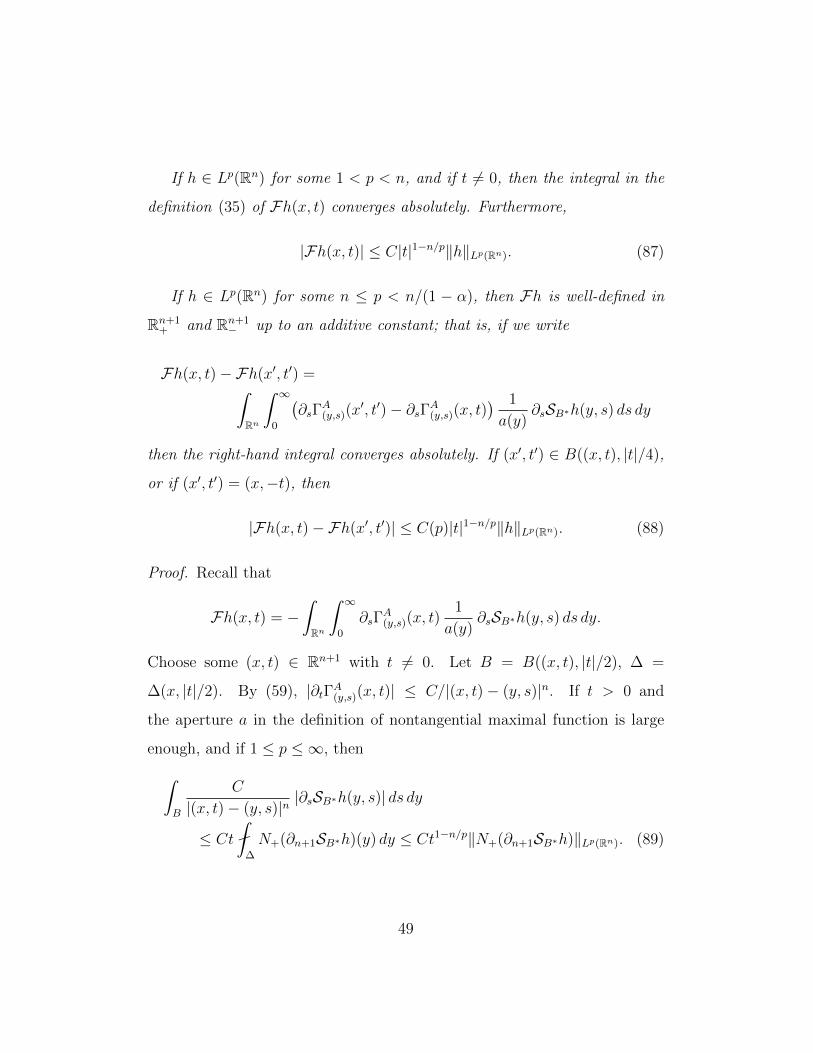
If h ∈ Lp(Rn) for some 1 < p < n, and if t 6= 0, then the integral in the

definition (35) of Fh(x, t) converges absolutely. Furthermore,

|Fh(x, t)| ≤ C|t|1−n/p‖h‖Lp(Rn). (87)

If h ∈ Lp(Rn) for some n ≤ p < n/(1 − α), then Fh is well-defined in

Rn+1+ and Rn+1

− up to an additive constant; that is, if we write

Fh(x, t)−Fh(x′, t′) =ˆRn

ˆ ∞0

(∂sΓ

A(y,s)(x

′, t′)− ∂sΓA(y,s)(x, t)) 1

a(y)∂sSB∗h(y, s) ds dy

then the right-hand integral converges absolutely. If (x′, t′) ∈ B((x, t), |t|/4),

or if (x′, t′) = (x,−t), then

|Fh(x, t)−Fh(x′, t′)| ≤ C(p)|t|1−n/p‖h‖Lp(Rn). (88)

Proof. Recall that

Fh(x, t) = −ˆRn

ˆ ∞0

∂sΓA(y,s)(x, t)

1

a(y)∂sSB∗h(y, s) ds dy.

Choose some (x, t) ∈ Rn+1 with t 6= 0. Let B = B((x, t), |t|/2), ∆ =

∆(x, |t|/2). By (59), |∂tΓA(y,s)(x, t)| ≤ C/|(x, t)− (y, s)|n. If t > 0 and

the aperture a in the definition of nontangential maximal function is large

enough, and if 1 ≤ p ≤ ∞, then

ˆB

C

|(x, t)− (y, s)|n|∂sSB∗h(y, s)| ds dy

≤ Ct

∆

N+(∂n+1SB∗h)(y) dy ≤ Ct1−n/p‖N+(∂n+1SB∗h)‖Lp(Rn). (89)

49

Observe that

ˆRn+1+ \B

C

|(x, t)− (y, s)|m|∂sSB∗h(y, s)| ds dy

≤ˆRn

N+(∂n+1SB∗h)(y)

ˆ ∞0

C

|x− y|m + (s+ |t|)mds dy. (90)

If m = n and 1 ≤ p < n, then these integrals converge and are at most

C(p)|t|1−n/p‖N+(∂n+1SB∗h)‖Lp(Rn).

By (64) we may bound ‖N+(∂n+1SB∗h)‖Lp(Rn) and (87) is proven.

To establish (88), recall that by (59) and (60), if |(x′, t′)− (x, t)| < |t|/4,

or if t > 0 and (x′, t′) = (x,−t), then for all (y, s) ∈ Rn+1+ \B we have that

|∂tΓA(y,s)(x, t)− ∂tΓA(y,s)(x′, t′)| ≤C|t|α

|(x, t)− (y, s)|n+α

Letting m = n + α, we see that if 1 < p < n/(1 − α) then the right-hand

side of (90) converges and is at most C(p)|t|1−n/p‖N+(∂n+1SB∗h)‖Lp(Rn). By

(64), and since (89) is valid for all 1 ≤ p ≤ ∞, this completes the proof of

(88).

Next, we consider ∇Fh and LAFh.

Lemma 91. Let a, A and B be as in Lemma 86. If h ∈ Lp(Rn) for some

1 < p < n/(1− α), then ∇Fh ∈ L2loc(R

n+1± ), and in particular, divA∇Fh is

a well-defined element of W 2−1,loc(R

n+1± ).

Furthermore,

−a divA∇Fh = ∂2n+1SB∗h in Rn+1

+ , (92)

divA∇Fh = 0 in Rn+1− (93)

in the weak sense.

50

As an immediate corollary, Eh is well-defined and also lies in W 21,loc(R

n+1± ),

and divA∇Eh = divA∇Fh in Rn+1± .

Proof. Fix some (x0, t0) ∈ Rn+1 with t0 6= 0, and let Br = B((x0, t0), r). Let

η be a smooth cutoff function, supported in B|t0|/2 and identically equal to 1

in B|t0|/4, with 0 ≤ η ≤ 1, |∇η| ≤ C/|t0|. For all (x, t) ∈ B|t0|/8, we have that

by definition of Fh and by (58),

Fh(x, t)−Fh(x0, t0)

=

ˆRn+1+

ΓA(y,s)(x, t)1

a(y)∂s(η(y, s)∂sSB∗h(y, s)

)ds dy

−ˆRn+1+

ΓA(y,s)(x0, t0)1

a(y)∂s(η(y, s)∂sSB∗h(y, s)

)ds dy

−ˆRn+1+

(∂sΓ

A(y,s)(x, t)− ∂sΓA(y,s)(x0, t0)

) 1− η(y, s)

a(y)∂sSB∗h(y, s) ds dy

= I(x, t)− I(x0, t0) + II(x, t).

If t0 < 0 then I ≡ 0. Otherwise, by (62), the function ∂n+1(η ∂n+1SB∗h) is

bounded and compactly supported, and so by Theorem 53, I ∈ Y 1,2(Rn+1) ⊂

W 21,loc(Rn+1). Furthermore, − divA∇I = (1/a)∂n+1(η ∂n+1SB∗h), and so

−a divA∇I = ∂2n+1SB∗h in B|t0|/8.

We must show that ∇II ∈ L2(B|t0|/8) and that divA∇II = 0 in B|t0|/8.

By (60) and Lemma 41, we have that if (y, s) /∈ B|t0|/4 then

ˆB|t0|/8

|∇x,t∂sΓA(y,s)(x, t)| dx dt ≤

C|t0|n+α

|(x0, t0)− (y, s)|n+α.

51

Thus by (90), if 1 < p < n/(1− α) then

ˆB|t0|/8

ˆRn+1+

|∇x,t∂sΓA(y,s)(x, t)|

1− η(y, s)

|a(y)||∂sSB∗h(y, s)| ds dy dx dt

≤ C(p)|t0|n−n/p‖N+(∂n+1SB∗h)‖Lp(Rn).

Thus by Fubini’s theorem,

∇II(x, t) =

ˆRn+1+

∇x,t∂sΓA(y,s)(x, t)

1− η(y, s)

a(y)∂sSB∗h(y, s) ds dy. (94)

If ϕ is a test function supported in B|t0|/8, then again by (60), (90) and the

Caccioppoli inequality,∣∣∣∣ˆRn+1

ϕ(x, t)∇II(x, t) dx dt

∣∣∣∣≤ C‖ϕ‖L2(Rn+1)|t0|1/2+n/2−n/p‖N+(∂n+1SB∗h)‖Lp(Rn)

and so ∇II(x, t) ∈ L2(B|t0|/8).

Finally, by the weak definition (14) of divA∇ and by the formula (94)

for ∇II, we have that divA∇II = 0 in B|t0|/8, as desired.

We conclude this section by proving the continuity of ∇Eh across the

boundary. This property is analogous to the continuity relations (66) for the

single layer potential, and is the reason we will eventually prefer the operator

E to F .

Lemma 95. Suppose that a, A and B are t-independent, a is accretive, A

satisfies the square-function estimate (32), and B∗ satisfies the single layer

potential requirements of Definition 33. Then there is a dense subset S ⊂

L2(Rn) such that if h ∈ S, then

limt→0+‖∇Eh( · , t)−∇Eh( · ,−t)‖L2(Rn) = 0.

52

Proof. We define the set S ⊂ L2(Rn) as follows. By assumption, S⊥,+B∗ is

invertible. Let S = (S⊥,+B∗ )−1(S ′), where h ∈ S ′ if h(x) = u(x, t) for some

t > 0 and some u with divB∗∇u = 0 in Rn+1+ and N+u ∈ L2(Rn).

We first show that S is dense. It suffices to show that S ′ is dense.

Choose some f ∈ L2(Rn). By well-posedness of (D)B∗

2 , there is some u

with divB∗∇u = 0 in Rn+1+ and u = f on ∂Rn+1

+ . Define fk ∈ L2(Rn) by

fk(x) = u(x, 1/k); then fk ∈ S ′. By Theorem 47, fk → f in L2(Rn), and so

S ′ is dense in L2(Rn).

Suppose that h ∈ S. Then S⊥,+B∗ h(x) = u(x, τ) for some τ > 0 and

some solution u. Let v(x, t) = ∂tu(x, t + τ). By (64), and by uniqueness

of solutions to (D)B∗

2 , we have that ∂tSh = v in Rn+1+ . But by the Cac-

cioppoli inequality and the De Giorgi-Nash-Moser estimates, we have that

N+(∂n+1v)(x) ≤ CτN+u(x) (possibly at the cost of increasing the apertures

of the nontangential cones).

So if h ∈ S, then

N+(∂2n+1SB∗h) ∈ L2(Rn).

Recall that by (34) and Lemma 86 if h ∈ L2(Rn) and n ≥ 3 then

Eh(x, t) = −ˆ ∞

0

ˆRn

∂sΓA(y,s)(x, t)

1

a(y)∂sSB∗h(y, s) dy ds−SA

(1

aS⊥,+B∗ h

)(x, t).

If n = 2 then we must instead work with Eh(x, t)− Eh(x,−t).

If h ∈ S, so that N+(∂2n+1SB∗h) ∈ L2(Rn), then we may integrate by

parts in the region 0 < s < τ for any fixed τ . Observe that the boundary

53

term at s = 0 precisely cancels the term SA((1/a)S⊥,+B∗ h). We conclude that

Eh(x, t) =

ˆ τ

0

ˆRn

ΓA(y,s)(x, t)1

a(y)∂2sSB∗h(y, s) dy ds

−ˆRn

ΓA(y,τ)(x, t)1

a(y)∂n+1SB∗h(y, τ) dy

−ˆ ∞τ

ˆRn

∂sΓA(y,s)(x, t)

1

a(y)∂sSB∗h(y, s) dy ds.

Applying (58) and the definition of SA, we see that

Eh(x, t) =

ˆ τ

0

SA(

1

a∂2sSB∗h(s)

)(x, t− s) ds− SA

(1

a∂τSB∗h(τ)

)(x, t− τ)

−ˆ ∞τ

∂sSA(

1

a∂sSB∗h(s)

)(x, t− s) ds.

Here we have adopted the notation that ∂sSB∗h(s)(y) = ∂sSB∗h(y, s).

Thus∇Eh(x, t)−∇Eh(x,−t) has three terms. Suppose that s ∈ R, s 6= 0.

By (64), ‖∂n+1SB∗h(s)‖L2(Rn) ≤ C‖h‖L2(Rn). Suppose that g ∈ L2(Rn). By

(81) and by (32),

‖∇SAg(s)‖L2(Rn) ≤ C‖N±(∇SAg)‖L2(Rn) ≤ C‖g‖L2(Rn).

Furthermore, if 0 < t < |s|/2, then by (83), (81) and (32),

‖∇SAg(s+ t)−∇SAg(s− t)‖L2(Rn) ≤ Ct

|s|‖g‖L2(Rn).

Finally by (83), (81), (32) and applying the Caccioppoli inequality to ∂n+1SA,

‖∇∂sSAg(s+ t)−∇∂sSAg(s− t)‖L2(Rn) ≤ Ct

|s|2‖h‖L2(Rn).

Thus, if t < τ , then

‖∇Eh(t)−∇Eh(−t)‖L2(Rn) ≤ C

ˆ τ

0

‖N+(∂2sSB∗h)‖L2(Rn) ds

+ Ct

τ‖h‖L2(Rn) + C

ˆ ∞τ

t

s2‖h‖L2(Rn) ds.

54

Choosing τ =√t and recalling that h ∈ S, we see that the right-hand side

goes to zero as t→ 0+, as desired.

6. A square-function bound

Recall that we intend to construct solutions to the Dirichlet problem (18)

by letting u = u+ + Eh for some appropriately chosen function h ∈ L2(Rn).

To prove Theorems 25 and 26 we must have that the norms ‖N+(∇Eh)‖L2(Rn)

and 9t∇∂tEh9+ are appropriately bounded.

In this section, we will prove a preliminary square-function estimate; we

will prove the full estimate ‖N+(∇Eh)‖L2(Rn) + 9t∇∂tEh9+ ≤ C‖h‖L2(Rn)

in the next section.

Theorem 96. Suppose that a, A and B are t-independent, a is accretive,

A, A∗, B and B∗ satisfy the De Giorgi-Nash-Moser condition, and SA, SB∗

satisfy the square-function estimate (31).

Then for all h ∈ L2(Rn), we have the bound

ˆ ∞−∞

ˆRn

|∂2tFh(x, t)|2 |t| dx dt ≤ C‖h‖2

L2(Rn).

In the remainder of this section, let u = ∂n+1SB∗h. Observe that

∂2tFh(x, t) = ∂2

t

ˆRn+1

∂tΓAT

(x,t)(y, s)1

a(y)u(y, s) dy ds.

By (32) and (63) it suffices to prove that

9t ∂2tFh9± ≤ C‖N+u‖L2(Rn) + C9t∇u9+. (97)

This theorem is the technical core of the paper. The proof is inspired by the

T (1) theorems of [? ] and [? ]. We may think of ∂2tFh(x, t) as Tu(x, t) for

55

a singular integral operator T with kernel (1/a(y)) ∂3t Γ

AT

(x,t)(y, s). The T (1)

theorem of Semmes was proven by analyzing Tu−T (1)Ptu and T (1)Ptu for an

averaging operator Pt. We will use the same argument; our operator Pt will

be averages over dyadic cubes. Our bound on T (1)Ptu will follow from well-

known Carleson-measure properties of solutions to second-order equations.

To bound Tu− T (1)Ptu in terms of ∇u, we develop an argument ultimately

allowing us to exploit the Poincare inequality. It bears some resemblance to

the arguments of [? ] (see, in particular, Lemma 3.5(i)), but the particular

singular integral operator at hand is different form those in [? ], and new

ideas are required.

For ease of notation we will prove (97) only in the upper half-space (that

is, only for 9t ∂2tFh9+); the argument in the lower half-space is similar and

simpler.

Let W be the grid of dyadic Whitney cubes in Rn+1+ . That is,

W = Q = Q× [`(Q), 2`(Q)) : Q ⊂ Rn is a dyadic cube.

Then Rn+1+ = ∪Q∈WQ, and any two distinct cubes Q, R ∈ W have disjoint

interiors. For any Q ∈ W we let F (Q) = R ∈ W : dist(R,Q) > 0 be the

set of cubes a positive distance from Q and let N(Q) = ∪R∈W\F (Q)R be the

union of cubes adjacent to Q.

Observe that

9t ∂2tFh9+ =

∑Q∈W

ˆQ

∣∣∣∣∂2t

ˆRn+1

∂tΓAT

(x,t)(y, s)1

a(y)u(y, s) dy ds

∣∣∣∣2 t dx dt.

56

If R ∈ W , let uR =fflRu. Define the four quantities

I =∑Q∈W

ˆQ

( ∑R∈F (Q)

ˆR

∣∣∣∂3t Γ

AT

(x,t)(y, s)1

a(y)

(u(y, s)− uR

)∣∣∣ dy ds)2

t dx dt,

II =∑Q∈W

ˆQ

( ∑R∈F (Q)

|uR − uQ|ˆR

∣∣∣∂3t Γ

AT

(x,t)(y, s)1

a(y)

∣∣∣ dy ds)2

t dx dt,

III =∑Q∈W

ˆQ

∣∣∣∣∂2t

ˆN(Q)

∂tΓAT

(x,t)(y, s)1

a(y)(u(y, s)− uQ) dy ds

∣∣∣∣2t dx dt,IV =

∑Q∈W

|uQ|2ˆQ

∣∣∣∣∂2t

ˆN(Q)

∂tΓAT

(x,t)(y, s)1

a(y)dy ds

+

ˆRn+1\N(Q)

∂3t Γ

AT

(x,t)(y, s)1

a(y)dy ds

∣∣∣∣2t dx dt.We have that

9t ∂2tFh9+ ≤ C(I + II + III + IV ).

We will bound each of the terms I, II, III and IV . We begin with

term IV .

Lemma 98. If a and A are t-independent, A and A∗ satisfy the De Giorgi-

Nash-Moser condition and SA satisfies the square-function bound (63), then

IV ≤ C‖N+u‖2L2(Rn)‖1/a‖2

L∞(Rn).

Proof. Recall that

IV =∑Q∈W

|uQ|2ˆQ

∣∣∣∣∂2t

ˆN(Q)

∂tΓAT

(x,t)(y, s)1

a(y)dy ds

+

ˆRn+1\N(Q)

∂3t Γ

AT

(x,t)(y, s)1

a(y)dy ds

∣∣∣∣2t dx dt.

57

By the decay estimate (59), both of the innermost integrals converge abso-

lutely. By (58), ∂tΓAT

(x,t)(y, s) = −∂sΓAT

(x,t)(y, s), and so

∂2t

ˆN(Q)

∂tΓAT

(x,t)(y, s)1

a(y)dy ds+

ˆRn+1\N(Q)

∂3t Γ

AT

(x,t)(y, s)1

a(y)dy ds

=

ˆRn

∂2t Γ

AT

(x,t)(y, 0)1

a(y)dy = ∂2

t SA(1/a)(x, t).

We claim that because 1/a ∈ L∞(Rn), we have that

dµ(x, t) = |∂2t SA (1/a) (x, t)|2 t dx dt

is a Carleson measure with Carleson norm ‖µ‖C at most C‖1/a‖2L∞(Rn). This

follows from the square-function bound (63) and the decay estimate (59) by

a simple argument due to Fefferman and Stein (see the proof of Theorem 3

in [? ]). Let R ⊂ Rn be a cube; then

ˆ `(R)

0

ˆR

|∂2t SA (1/a) (x, t)|2 t dx dt

≤ 2

ˆ `(R)

0

ˆR

|∂2t SA

(12R(1/a)

)(x, t)|2 t dx dt

+ 2

ˆ `(R)

0

ˆR

|∂2t SA

((1− 12R)(1/a)

)(x, t)|2 t dx dt.

The first integral is at most C‖1/a‖2L2(2R)

≤ C|R| ‖1/a‖2L∞(Rn) by (63), while

the second is at most C|R| ‖1/a‖2L∞(Rn) by (62).

Let uW (x, t) = uQ whenever (x, t) ∈ Q. Observe that N+uW (x) ≤

N+u(x) (possibly at a cost of increasing the aperture of nontangential cones).

Then

IV =

ˆRn+1+

|uW (x, t)|2 |∂2t SA(1/a)(x, t)|2 t dx dt.

58

Applying duality between Carleson measures and nontangentially bounded

functions, we see that

IV ≤ ‖N+((uW )2)‖L1(Rn)‖µ‖C ≤ C‖N+u‖2L2(Rn)‖1/a‖2

L∞(Rn)

as desired.

Next, we bound the term I.

Lemma 99. If a and A are t-independent, a is accretive, and A and A∗

satisfy the De Giorgi-Nash-Moser condition, then

I ≤ C

ˆRn+1+

|∇u(y, s)|2 s dy ds.

Proof. Recall that

I =∑Q∈W

ˆQ

( ∑R∈F (Q)

ˆR

∣∣∣∂3t Γ

AT

(x,t)(y, s)1

a(y)

(u(y, s)− uR

)∣∣∣ dy ds)2

t dx dt.

By the Poincare inequality,ˆR

|u(y, s)− uR| dy ds ≤ C`(R)

ˆR

|∇u(y, s)| dy ds.

By (59), and because `(R) ≤ s ≤ 2`(R) for any (y, s) ∈ R, we have that

I ≤∑Q∈W

ˆQ

( ∑R∈F (Q)

C`(R)‖1/a‖L∞(Rn)

dist(Q,R)n+2

ˆR

|∇u(y, s)| dy ds)2

t dx dt

≤ C‖1/a‖2L∞(Rn)

ˆRn+1+

(ˆRn+1+

s

(s+ t+ |x− y|)n+2|∇u(y, s)| dy ds

)2

t dx dt.

But by Holder’s inequality,ˆRn+1+

(ˆRn+1+

s

(s+ t+ |x− y|)n+2|∇u(y, s)| dy ds

)2

t dx dt

≤ˆRn+1+

ˆRn+1+

s2 |∇u(y, s)|2 dy ds(s+ t+ |x− y|)n+2

ˆRn+1+

dy ds

(s+ t+ |x− y|)n+2t dx dt

= C

ˆRn+1+

|∇u(y, s)|2s dy ds.(100)

59

This completes the proof.

We may bound III similarly.

Lemma 101. Suppose that a and A are as in Lemma 99. Suppose in addition

that B∗ is t-independent and satisfies the De Giorgi-Nash-Moser condition,

and divB∗∇u = 0 in Rn+1+ . Then

III ≤ C

ˆRn+1+

|∇u(y, s)|2 s dy ds.

Proof. Recall that

III =∑Q∈W

ˆQ

∣∣∣∣∂2t

ˆN(Q)

∂tΓAT

(x,t)(y, s)1

a(y)(u(y, s)− uQ) dy ds

∣∣∣∣2t dx dt.Observe that 2Q ⊂ N(Q) ⊂ 5Q. Let

w(x, t) =

ˆN(Q)

ΓAT

(x,t)(y, s)1

a(y)(u(y, s)− uQ) dy ds.

By (55), w satisfies |w(x, t)| ≤ C`(Q)2‖1/a‖L∞(Rn)‖u− uQ‖L∞(N(Q)).

By Theorem 53, aLAw = (u − uQ) in N(Q). If divB∗∇u = 0 in N(Q),

then L∗B(aLAw) = 0 in N(Q). Thus, we may use Theorem 73 and Corol-

lary 77 twice to show that

sup(x,t)∈Q

|∂3tw(x, t)| ≤ C

`(Q)‖1/a‖L∞(Rn)‖u− uQ‖L∞(N(Q))

and so

III ≤∑Q∈W

ˆQ

(C

`(Q)‖1/a‖L∞(Rn)‖u− uQ‖L∞(N(Q))

)2

t dx dt.

Let

π(Q) = x : (x, t) ∈ Q for some t > 0

60

be the projection of Q onto Rn. Notice that π(Q) is also a cube. Let U(Q) =

6π(Q) × (`(Q)/4, 5`(Q)). Observe that if X ∈ N(Q), then B(X, `(Q)/4) ⊂

U(Q). If divB∗∇u = 0 in U(Q), then by the De Giorgi-Nash-Moser condition

and the Poincare inequality,

supN(Q)

|u− uQ| ≤ C

( U(Q)

|u− uQ|2)1/2

≤ C`(Q)

( U(Q)

|∇u|2)1/2

.

So

III ≤ C‖1/a‖2L∞(Rn)

∑Q∈W

ˆQ

U(Q)

|∇u(y, s)|2 dy ds t dx dt.

Because each (y, s) ∈ Rn+1 lies in U(Q) for at most C cubes Q ∈ W , this

implies that

III ≤ C‖1/a‖2L∞(Rn)

ˆRn+1+

|∇u(y, s)|2 s dy ds

as desired.

Finally, we come to the term II.

Lemma 102. If a is accretive, and if A and A∗ are t-independent and satisfy

the De Giorgi-Nash-Moser condition, then

II ≤ C

ˆRn+1+

(ˆRn+1+

s

(s+ t+ |x− y|)n+2|∇u(y, s)| dy ds

)2

t dx dt. (103)

Note that the estimate (103) together with (100) above imply that

II ≤ C

ˆRn+1+

|∇u(y, s)|2s dy ds.

Proof. Recall that

II =∑Q∈W

ˆQ

( ∑R∈F (Q)

|uR − uQ|ˆR

∣∣∣∂3t Γ

AT

(x,t)(y, s)1

a(y)

∣∣∣ dy ds)2

t dx dt.

61

To analyze the inner sum, we establish some notation. As in the proof of

Lemma 101, if R ∈ W is a cube, we let π(R) be the projection of R onto Rn.

We let P (R) denote the Whitney cube directly above R, so π(P (R)) is the

dyadic parent of π(R). Let δ(Q,R) = `(Q) + `(R) + dist(π(Q), π(R)). If

(x, t) ∈ Q and (y, s) ∈ R for some R ∈ F (Q), then

|(y, s)− (x, t)| ≈ |x− y|+ max(s, t) ≈ δ(Q,R).

Here U ≈ V if U ≤ CV and V ≤ CU . Applying (59), we see that

II ≤ C∑Q∈W

ˆQ

(∑R∈W

|uR − uQ||R|

δ(Q,R)n+2

)2

t dx dt.

To analyze the sum over R ∈ W , we will divide W into a “discretized

cone” over Q and a leftover region. Let G′(Q) be the discretized cone given

by

G′(Q) = R ∈ W : `(R) > `(Q), `(R) > dist(π(R), π(Q)).

Let G(Q) be the larger discretized cone given by

G(Q) = R ∈ W : P (R) ∈ G′(Q).

Let B(Q) = G(Q) \ G′(Q) be the lower boundary of G(Q). If R is a cube,

let T (R) be the set of cubes below R, that is,

T (R) = S ∈ W : π(S) ( π(R).

Observe that if R, S ∈ B(Q) are distinct cubes then their projections π(R)

and π(S) are disjoint, and so if R ∈ B(Q) then T (R) ∩ G(Q) is empty.

Furthermore, if S is a Whitney cube, then either S ∈ G(Q) or S ∈ T (R) for

a unique cube R ∈ B(Q).

62

Thus, we may write

II ≤ C∑Q∈W

ˆQ

( ∑R∈G(Q)

|uR − uQ||R|

δ(Q,R)n+2

)2

t dx dt

+ C∑Q∈W

ˆQ

( ∑R∈B(Q)

∑S∈T (R)

|uS − uQ||S|

δ(Q,S)n+2

)2

t dx dt.

We may write |uS − uQ| ≤ |uS − uR|+ |uR − uQ| in the second sum. Observe

that if R ∈ B(Q) = G(Q)\G′(Q), then R is not in G′(Q) but the cube P (R)

above it is, and so either `(R) ≈ `(Q) or `(R) ≈ dist(π(R), π(Q)). Thus if

S ∈ T (R) then δ(S,Q) ≈ `(R) ≈ δ(R,Q). So we may write

II ≤ C∑Q∈W

ˆQ

( ∑R∈G(Q)

|uR − uQ||R|

δ(Q,R)n+2

)2

t dx dt

+ C∑Q∈W

ˆQ

( ∑R∈B(Q)

∑S∈T (R)

|uS − uR||S|

δ(Q,R)n+2

)2

t dx dt

= C(V + V I).

We begin by analyzing the term V I. Choose some R ∈ B(Q). Let

L0 = R, and let Lj = S ∈ T (R) : `(S) = 2−j`(R). Then

∑S∈T (R)

|uS − uR| |S| = |R|∞∑j=1

2−j(n+1)∑S∈Lj

|uS − uR|.

Let Uj =∑

S∈Lj|uS − uR|; observe that U0 = 0. Then for each j ≥ 1,

Uj =∑S∈Lj

|uS − uR| ≤∑S∈Lj

|uS − uP (S)|+∑S∈Lj

|uP (S) − uR|.

The second term is equal to 2nUj−1. To contend with the first term, we apply

63

the Poincare inequality in the set S ∪ P (S). Then

|uS − uP (S)| ≤ |uS − uS∪P (S)|+ |uP (S) − uS∪P (S)|

=1

|S|

ˆS

|u− uS∪P (S)|+1

2n|S|

ˆP (S)

|u− uS∪P (S)|

≤ 1

|S|

ˆS∪P (S)

|u− uS∪P (S)| ≤ C`(S)

|S|

ˆS∪P (S)

|∇u(y, s)| dy ds.

Thus,

Uj ≤ 2nUj−1 +∑S∈Lj

C

`(S)n

ˆS

|∇u|+ 22n∑

S∈Lj−1

C

`(S)n

ˆS

|∇u|.

Since U0 = 0, by induction

Uj ≤j−1∑k=0

(2n + 1)2n(j−k)∑S∈Lk

C

`(S)n

ˆS

|∇u|+∑S∈Lj

C

`(S)n

ˆS

|∇u|

which may be simplified to

Uj ≤ C

j∑k=0

2n(j−k)∑S∈Lk

1

`(S)n

ˆS

|∇u|.

Thus∑S∈T (R)

|uS − uR| |S| = |R|∞∑j=1

2−j(n+1)Uj

≤ |R|∞∑j=1

2−j(n+1)

j∑k=0

2n(j−k)∑S∈Lk

C

`(S)n

ˆS

|∇u(y, s)| dy ds

= |R|∞∑k=0

2−k−nk∑S∈Lk

C

`(S)n

ˆS

|∇u(y, s)| dy ds

≤ C∑

S∈T (R)∪R

`(S)

ˆS

|∇u(y, s)| dy ds.

64

So

V I =∑Q∈W

ˆQ

( ∑R∈B(Q)

1

δ(Q,R)n+2

∑S∈T (R)

|uS − uR| |S|)2

t dx dt

≤ C∑Q∈W

ˆQ

( ∑R∈B(Q)

1

δ(Q,R)n+2

∑S∈T (R)∪R

`(S)

ˆS

|∇u(y, s)| dy ds)2

t dx dt

≤ C

ˆRn+1+

(ˆRn+1+

s

(t+ s+ |x− y|)n+2|∇u(y, s)| dy ds

)2

t dx dt

because δ(Q,R) ≈ δ(Q,S) ≈ t+s+ |x− y| for any S ∈ T (R), any R ∈ B(Q)

and any (x, t) ∈ Q and (y, s) ∈ S.

Now, recall that

V =∑Q∈W

ˆQ

( ∑R∈G(Q)

|uR − uQ||R|

δ(Q,R)n+2

)2

t dx dt.

Observe that if R ∈ G(Q) then dist(π(R), π(Q)) ≤ C`(R) and so δ(R,Q) ≈

`(R); thus

V ≤ C∑Q∈W

ˆQ

( ∑R∈G(Q)

|uR − uQ|1

`(R)

)2

t dx dt.

Let Gj(Q) = R ∈ G(Q) : `(R) = 2j`(Q). Let xQ be the midpoint of the

cube π(Q). There is some constant c depending only on dimension such that

if R ∈ Gj(Q) then R is contained in the cylinder Cj(Q) = ∆(xQ, c 2j`(Q))×

(2j`(Q), 2j+1`(Q)). Therefore,∑R∈Gj(Q)

|uR − uQ| =1

2j(n+1)|Q|∑

R∈Gj(Q)

ˆR

|u(y, s)− uQ| dy ds

≤ C

Cj(Q)

|u(y, s)− uCj(Q)| dy ds+ C|uCj(Q) − uQ|.

65

If j ≥ 1, then

|uCj(Q) − uQ| ≤ |uC0(Q) − uQ|+j∑

k=1

|uCk(Q) − uCk−1(Q)|.

Applying the Poincare inequality in Ck(Q) ∪ Ck−1(Q), we see that

|uCk(Q) − uCk−1(Q)| ≤C

2kn`(Q)n

ˆCk(Q)∪Ck−1(Q)

|∇u(y, s)| dy ds.

Observe that Q ⊂ C0(Q), and so by the Poincare inequality,

|uC0(Q) − uQ| ≤ C `(Q)

C0(Q)

|∇u(y, s)| dy ds.

Finally,fflCj(Q)|u(y, s)− uCj(Q)| dy ds ≤ C2j`(Q)

fflCj(Q)|∇u(y, s)| dy ds. So

∑R∈Gj(Q)

|uR − uQ| ≤j∑

k=0

C

2kn`(Q)n

ˆCk(Q)

|∇u(y, s)| dy ds.

Thus,∑R∈G(Q)

1

`(R)|uR − uQ| =

∞∑j=0

1

2j`(Q)

∑R∈Gj(Q)

|uR − uQ|

≤∞∑j=0

1

2j`(Q)

j∑k=0

C

2kn`(Q)n

ˆCk(Q)

|∇u(y, s)| dy ds

= C∞∑k=0

2k`(Q)

2k(n+2)`(Q)n+2

ˆCk(Q)

|∇u(y, s)| dy ds.

But if (y, s) ∈ Ck(Q) and (x, t) ∈ Q, then |x− y| + t ≤ C2k`(Q) and s ≈

2k`(Q). Thus,

V ≤ C∑Q∈W

ˆQ

( ∑R∈G(Q)

|uR − uQ|1

`(R)

)2

t dx dt

≤ C∑Q∈W

ˆQ

( ∞∑k=0

2k`(Q)

2k(n+2)`(Q)n+2

ˆCk(Q)

|∇u(y, s)| dy ds)2

t dx dt

≤ C

ˆRn+1+

(ˆRn+1+

s

(|x− y|+ t+ s)n+2|∇u(y, s)| dy ds

)2

t dx dt.

66

This completes the proof.

7. A nontangential bound

We have established that, if h ∈ L2(Rn), then under appropriate assump-

tions on a, A and B,

ˆRn

ˆ ∞0

|∂2tFh(x,±t)|2t dt dx ≤ C‖h‖2

L2(Rn). (104)

In this section we will prove that, if h ∈ L2(Rn), then under appropriate

assumptions on a, A and B,

9t∇∂tEh)9+ + ‖N+(∇Eh)‖L2(Rn) ≤ C‖h‖2L2(Rn).

Recall that Eh = Fh − SA(

1aS⊥,+B∗ h

); thus by (32) and (63), the difference

Eh−Fh satisfies square-function estimates and nontangential estimates, and

so we may work with E or F , whichever is more convenient.

This proof will require several steps.

Lemma 105. Suppose that v ∈ W 21,loc(R

n+1± ) satisfies the conditions of Lem-

ma 80, that is, that v, ∂n+1v and ∂2n+1v satisfy the Caccioppoli inequality

in Rn+1± .

Suppose furthermore that there is a constant C1 such that

‖∇v( · , t)‖L2(Rn) ≤ C1|t|−1. (106)

Then there is some constant C, depending only on the constants in the Cac-

cioppoli inequality, such that

ˆ ∞0

ˆRn

|∇v(x,±t)|2 t dx dt ≤ C

ˆ ∞0

ˆRn

|∂tv(x,±t)|2 t dx dt+ C21 .

67

We will immediately apply this lemma to ∂tFh in the lower half-space.

Later in Corollary 115, we will apply this lemma to ∂tEh in the upper half-

space as well. The bound (106) is simpler to establish in the lower half-space

because Fh(x, t) is defined in terms of an integral over Rn+1+ , and certain

direct bounds can be computed if (x, t) does not lie in the integrand.

Proof. This parallels the proof of [? , Formula (5.5)], where a similar in-

equality was proven for the single layer potential.

Define um(t) =´Rn|∇∂mt v(x,±t)|2 dx. Observe that by assumption u0(t) ≤

C21 t−2, and by the Caccioppoli inequality,

ˆ ∞0

t3 u1(t) dt =

ˆRn+1+

|∇∂tv(x,±t)|2 t3 dx dt ≤ C

ˆRn+1+

|∂tv(x,±t)|2 t dx dt.

We wish to bound´∞

0t u0(t) dt.

Suppose t > 0. By (83), u0 is locally Lipschitz continuous. Thus if

0 < ε < S <∞, then

ˆ S

ε

t u0(t) dt =

ˆ S

ε

t u0(S) dt−ˆ S

ε

t

ˆ S

t

u′0(s) ds dt

≤ C21

2+

1

2

ˆ S

ε

s2 |u′0(s)| ds.

But |u′0(s)| ≤ 2√u0(s)u1(s) and so

ˆ S

ε

t u0(t) dt ≤ C21

2+

ˆ S

ε

s2√u0(s)u1(s) ds

≤ C21

2+

1

2

ˆ S

ε

s u0(s) ds+1

2

ˆ S

ε

s3 u1(s) ds.

Rearranging terms, we have that

ˆ S

ε

t u0(t) dt ≤ C21 +

ˆ S

ε

s3 u1(s) ds.

68

Taking the limit as ε→ 0+ and S →∞, we have that

ˆ ∞0

ˆRn

|∇v(x,±t)|2 t dx dt =

ˆ ∞0

t u0(t) dt ≤ C21 +

ˆ ∞0

t3 u1(t) dt

≤ C21 + C

ˆ ∞0

ˆRn

|∂tv(x,±t)|2 t dx dt

as desired.

We now proceed to nontangential estimates in the lower half-space.

Lemma 107. Suppose that a, A and B are t-independent, a is accretive,

A satisfies the single layer potential requirements of Definition 33, B and

B∗ satisfy the De Giorgi-Nash-Moser condition and SB∗ satisfies the square-

function estimate (31).

Then for every h ∈ L2(Rn), we have that

‖N−(∇Eh)‖L2(Rn) ≤ C‖h‖L2(Rn) (108)

and the boundary value ∇Eh∣∣∂Rn+1−

exists in the sense of (16).

Proof. By the definitions (35) and (29) of F and SA,

∇∂tFh(x,−t) = −ˆ ∞

0

∇∂2t SA

(1

a∂sSB∗h(s)

)(x,−t− s) ds (109)

where as in the proof of Lemma 95 we let SB∗h(s)(y) = SB∗h(y, s). Because

A and B∗ are t-independent and have bounded layer potentials, if t > 0,

then by (43), (64) and the Caccioppoli inequality, ‖∇∂tFh( · ,−t)‖L2(Rn) ≤

Ct−1‖h‖2L2(Rn). Thus by Lemma 105,

ˆ ∞0

ˆRn

|∇∂tFh(x,−t)|2 t dx dt ≤ C

ˆ ∞0

ˆRn

|∂2tFh(x,−t)|2 t dx dt+C‖h‖2

L2(Rn).

By Theorem 96 this is at most C‖h‖2L2(Rn).

69

Since divA∇(∂tFh) = 0 in Rn+1− , we may apply Theorem 46 in the lower

half-space. Thus

‖N−(∂tFh)‖2L2(Rn) ≤

ˆRn+1+

|∇∂tFh(x,−t)|2 t dx dt ≤ C‖h‖2L2(Rn) (110)

and the boundary value

F⊥,−h = ∂n+1Fh∣∣∂Rn+1−

exists in the sense of L2 functions.

Because A satisfies the single layer potential requirements, S⊥,−A is invert-

ible L2(Rn) 7→ L2(Rn), and so there is some g ∈ L2(Rn) with S⊥,−A g = F⊥,−h.

Furthermore, ‖g‖L2(Rn) ≤ C‖h‖L2(Rn).

By (64), if u = ∂n+1SAg, then ‖N−u‖L2(Rn) < ∞. By (110) the same is

true of u = ∂n+1Fh, and so by uniqueness of solutions to (D)A2 , we have that

∂n+1SAg = ∂n+1Fh in Rn+1− . By (32), and by (88) and Theorem 73, we have

that u = SAg − Fh satisfies the conditions of Lemma 49, and so SAg = Fh

in Rn+1− up to an additive constant.

In particular, by (32) we have that

‖N−(∇Fh)‖L2(Rn) ≤ C‖h‖L2(Rn).

By definition of Eh and by (32), (108) is valid. By Theorem 47, and because

divA∇(Eh) = 0 in Rn+1− , we have that ∇Eh|∂Rn+1

−exists and lies in L2(Rn).

Lemma 111. Suppose that a, A and B are as in Lemma 86. Let h ∈ L2(Rn).

Then

‖N+(∂tEh)‖L2(Rn) ≤ C‖N−(∂tEh)‖L2(Rn) + C‖h‖L2 .

70

Proof. This is essentially the analogue to Cotlar’s inequality for singular

integral operators (see, for example, [? , (8.2.2)]) reformulated to apply to

our potential E . We prove it using similar arguments.

Let x∗ ∈ Rn and let (x, t) ∈ γ+(x∗) for some t > 0, where γ+ is the

nontangential cone given by (8). There is some constant j0, depending on

the aperture a of the nontangential cones, such that x ∈ ∆(x∗, 2j0t). Let A0 =

∆0 = ∆(x∗, 2j0+1t), and for each j ≥ 1, let Aj be the annulus ∆(x∗, 2j0+j+1t)\

∆(x∗, 2j0+jt). Let hj = h1Aj, so h =

∑∞j=0 hj. Then

|∂n+1Eh(x, t)| ≤ |∂n+1Eh(x,−t)|+∞∑j=0

|∂n+1Ehj(x, t)− ∂n+1Ehj(x,−t)|.

Observe that |∂tEh(x,−t)| ≤ N−(∂n+1Eh)(x∗). By (87) and Corollary 77, if

1 < p < n then

|∂tFhj(x, t)|+ |∂tFhj(x,−t)| ≤C

tn/p‖hj‖Lp(Rn) ≤ C2jn/pM(|h|p)(x∗)1/p

where M denotes the Hardy-Littlewood maximal function. Recall that

Ehj(x, τ) = Fhj(x, τ)− SA(

1

aS⊥,+B∗ hj

)(x, τ)

= −ˆRn+1+

∂sΓA(y,s)(x, τ)

1

a(y)∂sSB∗hj(y, s) ds dy − SA

(1

aS⊥,+B∗ hj

)(x, τ).

Applying (62) to SA and (64) to S⊥,+B∗ , we see that the same is true of ∂tEhj.

We will apply this bound only for j = 0 and j = 1; we seek a better bound

for j ≥ 2.

Suppose j ≥ 2. Let Aj = Aj−1 ∪ Aj ∪ Aj+1. We divide Rn+1+ into three

pieces: I = Aj × (0, 2jt), II = Aj × (2jt,∞) and III = (Rn \ Aj)× (0,∞).

We integrate by parts in s in II and III. Recalling the definition of SA, we

71

have that

∂τEhj(x, τ) =

ˆI

∂2sΓ

A(y,s)(x, τ)

1

a(y)∂sSB∗hj(y, s) ds dy

−ˆII∪III

∂sΓA(y,s)(x, τ)

1

a(y)∂2sSB∗hj(y, s) ds dy

+

ˆAj

∂τΓA(y,2jt)(x, τ)

1

a(y)∂n+1SB∗hj(y, 2jt) dy

− ∂τSA(

1Aj

1

aS⊥,+B∗ hj

)(x, τ).

Thus ∂n+1Ehj(x, t)− ∂n+1Ehj(x,−t) may be written as a sum of four terms.

Applying the bound (64) on SB∗ , the bound (62) and Holder continuity to

SA and SB∗ , and the bounds (59) and (60) on ΓA(y,s)(x, τ), we may show that

each term is at most C2−jαM(|h|p)(x∗)1/p.

Thus, if 1 < p < n then

|∂tEh(x, t)| ≤ N−(∂n+1Eh)(x∗) +∞∑j=0

C2−jαM(|h|p)(x∗)1/p.

Choosing 1 < p < 2 and recalling that M is bounded Lp 7→ Lp for any

1 < p <∞, we have that

‖N+(∂n+1Eh)‖L2(Rn) ≤ ‖N−(∂n+1Eh)‖L2(Rn) + C‖h‖L2(Rn)

as desired.

Lemma 112. Suppose that a, A and B are t-independent, that a is accre-

tive, and that A and B∗ satisfy the single layer potential requirements of

Definition 33. Then for all h ∈ L2(Rn),

‖N+(∇Eh)2‖L2(Rn) ≤ C‖h‖L2(Rn) (113)

72

and ∇Eh|∂Rn+1+

exists and satisfies

∇Eh∣∣∂Rn+1

+= ∇Eh

∣∣∂Rn+1−. (114)

Proof. First, assume that h ∈ S where S is as in Lemma 95. By Lemmas 95

and 107, the formula (114) is valid, and so we may define E±h = Eh|∂Rn+1±

.

Let x∗ ∈ Rn and let (x, t) ∈ γ(x∗). By Theorem 73 and Corollary 79, we

have that B((x,t),t/2)

|∇Eh|2 ≤ C

r2

B((x,t),5t/8)

|Eh− E|2 ≤ C

r2

( B((x,t),3t/4)

|Eh− E|)2

for any constant E.

If (y, s) ∈ Rn+1+ , then

|Eh(y, s)− E| ≤ |Eh(y, s)− E+h(y)|+ |E+h(y)− E|

≤ sN+(∂n+1Eh)(y) + |E+h(y)− E|.

Let ∆ = ∆(x∗, Ct) where C is large enough that ∆(x, t) ⊂ ∆(x∗, Ct). Then

B((x,t),t/2)

|∇Eh|2 ≤ C

t2

( ∆

tN+(∂n+1Eh)(y) + |E+h(y)− E| dy)2

≤ C

( ∆

N+(∂n+1Eh)(y) dy

)2

+C

r2

( ∆

|E+h(x)− E| dx)2

.

Choose E =ffl

∆Eh(x, 0) dx and apply the Poincare inequality. We conclude

that

N+(∇Eh)(x∗)2 = sup(x,t)∈γ(x∗)

B((x,t),t/2)

|∇Eh|2

≤ CM(N+(∂tEh))(x∗)2 + CM(∇‖E+h)(x∗)2.

By Lemma 107 and Lemma 111, and by the L2-boundedness of the Hardy-

Littlewood maximal operator, we have that (113) is valid for all h ∈ S.

73

We now must pass to arbitrary h ∈ L2(Rn). Define

Nδ,RF (x) = sup

( B((y,s),s/2)

|F |2)1/2

: (y, s) ∈ γ+(x), δ < s < R, |y| < R

.

By (87), (62) and Theorem 73, for any fixed δ > 0, R < ∞ the map h 7→

Nδ,R(∇Eh) is continuous on L2(Rn). Thus because S is dense in L2(Rn), we

have that for any h ∈ L2(Rn),

‖Nδ,R(∇Eh)‖L2(Rn) ≤ C‖h‖L2(Rn)

uniformly in δ, R. Letting δ → 0 and R→∞ establishes (113). Recall that

(114) is valid for all h ∈ S. By (113) and Lemma 80, we may extend (114)

to all of L2(Rn).

Corollary 115. Suppose that a, A and B are as in Lemma 112. If h ∈

L2(Rn), thenˆ ∞

0

ˆRn

|∇∂tEh(x, t)|2 t dx dt ≤ C‖h‖2L2(Rn).

Proof. By Theorem 96, (31) and the L2-boundedness of S⊥,+B∗ , we have thatˆ ∞

0

ˆRn

|∂2t Eh(x, t)|2 t dx dt ≤ C‖h‖2

L2(Rn).

By Lemmas 80 and 112, we have that

‖∇∂tEh( · , t)‖L2(Rn) ≤C

t‖N+(∇Eh)‖L2(Rn) ≤

C

t‖h‖L2(Rn)

and so the conclusion follows from Lemma 105.

8. The proof of the main theorem

In this section, we will first prove an invertibility result for the potential

E = EB,a,A. We will use this invertibility result to prove existence of solutions

74

to the fourth-order Dirichlet problem. Finally, we will conclude this paper

by proving uniqueness of solutions and establishing a Fatou-type theorem.

We remark that the invertibility argument and the construction of so-

lutions in this section closely parallels the construction of solutions for the

biharmonic Dirichlet problem of [? ] and [? ].

The invertibility result we will prove is the following.

Lemma 116. Suppose that a, A and B are t-independent, that a is accretive

and that A and A∗ satisfy the single layer potential requirements of Defini-

tion 33. Then there is some ε > 0 and some C > 0, depending only on the

parameters listed in Theorem 25, such that if

‖Im a‖L∞(Rn) + ‖A−B‖L∞(Rn) < ε

then the mapping h 7→ ∂n+1EB,a,Ah|∂Rn+1±

is invertible on L2(Rn), and its

inverse has norm at most C.

Proof. Define E⊥B,a,Ah = ∂n+1EB,a,Ah|∂Rn+1−

. We begin by showing that E⊥A,a,Ais invertible for a real; it is for this reason that we require that both A and

A∗ satisfy the single layer potential requirements.

Choose some h ∈ S, where S ⊂ L2(Rn) is as in Lemma 95. By definition

of the single layer potential,ˆRn

g(x) ∂tFA,a,Ah(x,−t) dx =

ˆRn

ˆ ∞0

∂2t SAT g(y, s+t)

1

a(y)∂sSA∗h(y, s) ds dy.

Integrating by parts and applying the dominated convergence theorem yields

thatˆRn

g(x) E⊥A,a,Af(x) dx = − limt→0−

ˆRn

ˆ ∞0

∂sSAT g(y, s− t) 1

a(y)∂2sSA∗f(y, s) ds dy

=

ˆRn

S⊥,+AT g(y)

1

a(y)S⊥,+A∗ f(y) dy −

ˆRn

f(x) E⊥A,a,A

g(x) dx.

75

By density of S and by the L2-boundedness of E⊥A,a,A and E⊥A,a,A

, we have that

for any h ∈ L2(Rn),

ˆRn

h E⊥A,a,Ah+

ˆRn

h E⊥A,a,A

h =

ˆRn

1

a(y)S⊥,+AT h(y)S⊥,+A∗ h(y) dy.

Observe that EA,a,Ah(x, t) = EA,a,Ah(x, t). Thus, if a is real, then

ˆRn

h E⊥A,a,A

h dσ =

ˆRn

h E⊥A,a,Ah dσ

and so

Re

ˆRn

h E⊥A,a,Ah dσ =1

2

ˆRn

1

a(Y )|S⊥,+A∗ h(y)|2 dσ(Y ) ≥ 1

C‖S⊥,+A∗ h‖

2L2(Rn).

Thus because A∗ satisfies the single layer potential requirements,∣∣∣∣ˆRn

h E⊥A,a,Ah dσ∣∣∣∣ ≥ 1

C‖h‖2

L2(Rn)

and so E⊥A,a,A must be one-to-one. But the adjoint (E⊥A,a,A)∗ must also be one-

to-one, and so E⊥A,a,A must be invertible. Furthermore, (E⊥A,a,A)−1 is bounded

L2(Rn) 7→ L2(Rn), as desired.

We prove invertibility for ‖Im a‖L∞ or ‖A−B‖L∞ small using standard

analyticity arguments. Specifically, the mapping a 7→ E⊥A,a,A is analytic in

the sense that if z 7→ az is analytic D 7→ L∞(Rn) for some D ⊂ C, then z 7→

E⊥A,az ,Ah is analytic D 7→ L2(Rn) for any h ∈ L2(Rn). Furthermore, under

our assumptions, if a0 is real and accretive then ‖E⊥A,a,Ah‖L2(Rn) is bounded

for all t-independent a in a L∞ neighborhood of a0; thus if ‖a− a0‖L∞ is

small enough, then

‖E⊥A,a,A − E⊥A,a0,A‖L2(Rn)7→L2(Rn) ≤ C‖a− a0‖L∞(Rn).

76

Thus, if ‖Im a‖L∞(Rn) is small enough then E⊥A,a,A is invertible on L2(Rn).

Similarly, invertibility of E⊥B,a,A for ‖A−B‖L∞(Rn) small enough follows from

analyticity of the map B 7→ ΓBX .

We now use this invertibility result to prove existence of solutions to the

fourth-order Dirichlet problem.

Theorem 117. Suppose that a, A and B satisfy the conditions of Lem-

ma 116. Let f ∈ W 21 (Rn) and let g ∈ L2(Rn).

Then there exists a constant c and an h ∈ L2(Rn), with ‖h‖L2(Rn) ≤

C‖∇f‖L2(Rn) + C‖g‖L2(Rn), such that

u(X) = −DAf(X)− SAg(X) + EB,a,Ah(X) + c

satisfies L∗B(aLAu) = 0 in Rn+1

+ ,

u = f on ∂Rn+1+ ,

~e · A∇u = g on ∂Rn+1+

where L∗B(aLAu) = 0 in the sense of Definition 15 and where u = f , ~e ·

A∇u = g in the sense that

limt→0+‖u( · , t)− f‖W 2

1 (Rn) + ‖~e · A∇u( · , t)− g‖L2(Rn) = 0.

Furthermore,

‖N+(∇u)‖L2(Rn) + 9t LAu9+ + 9t∇∂tu9+ ≤ C‖∇f‖L2(Rn) + C‖g‖L2(Rn).

(118)

77

Proof. Let v(X) = −DAf(X)− SAg(X), so that divA∇v = 0 in Rn+1 \ Rn.

By (69) and (32), and by (70) and (63), we have that

‖N±(∇v)‖L2(Rn) + 9t∇∂tv9 ≤ C‖∇f‖L2(Rn) + C‖g‖L2(Rn). (119)

By Theorem 47, ∂n+1v|∂Rn+1−

exists and lies in L2(Rn). Let h ∈ L2(Rn) be

such that

∂n+1EB,a,Ah∣∣∂Rn+1−

= −∂n+1v|∂Rn+1−.

By Lemma 116, h exists and satisfies ‖h‖L2(Rn) ≤ C‖∇f‖L2(Rn) +C‖g‖L2(Rn).

Thus by Lemma 112 and Corollary 115,

‖N±(∇EB,a,Ah)‖L2(Rn)+9t∇∂tEB,a,Ah9 ≤ C‖∇f‖L2(Rn)+C‖g‖L2(Rn). (120)

By (92), LAEB,a,Ah = (1/a)∂2n+1SB∗h and so by (31),

9t LAEB,a,Ah9+ ≤ C‖h‖L2(Rn) ≤ C‖∇f‖L2(Rn) + C‖g‖L2(Rn).

Let w = v + EB,a,Ah = −DAf − SAg + EB,a,Ah. Then w satisfies (118).

By (92), L∗B(aLAw) = 0 in Rn+1+ in the sense of Definition 15. We need only

show that for some constant c, u = w + c has the correct boundary values.

By our choice of h, ∂n+1w = 0 on ∂Rn+1− . By (119) and (120), ∂n+1w is a

(D)A2 -solution in Rn+1− , and so ∂n+1w = 0 in Rn+1

− . Again by (119) and (120),

w satisfies the conditions of Lemma 49, and so w is constant in Rn+1− .

By (65), (66), (71), and (72),

limt→0+∇‖v( · , t)−∇‖v( · ,−t) = ∇f, lim

t→0+~e ·A∇v( · , t)− ~e ·A∇v( · ,−t) = g

in L2(Rn), and by (114) the same is true of w. Since w is constant in Rn+1− ,

this yields that ~e·A∇w|∂Rn+1+

= g and that∇‖w|∂Rn+1+

= ∇f . As in Remark 24

we have that w → f − c, for some constant c, pointwise nontangentially and

in L2(Rn). Letting u = w + c completes the proof.

78

We conclude this paper by proving a Fatou-type theorem and uniqueness

of solutions.

Theorem 121. Suppose that a, A and B are t-independent, that a is ac-

cretive, and that A and B∗ satisfy the single layer potential requirements of

Definition 33. We do not require that ‖Im a‖L∞ or ‖A−B‖L∞ be small.

Suppose that u satisfies L∗B(aLAu) = 0 in Rn+1+ ,

‖N+(∇u)‖L2(Rn) + 9t LAu9+ <∞.

Then ~G = ∇u|∂Rn+1+

exists in the sense of (16) and satisfies

‖~G‖L2(Rn) ≤ C‖N+(∇u)‖L2(Rn) + C9t LAu9+. (122)

Furthermore, there exist functions uA ∈ W 21,loc(R

n+1+ ) and h ∈ L2(Rn)

that satisfy the estimate

‖N+(∇uA)‖L2(Rn) + ‖h‖L2(Rn) ≤ C‖N+(∇u)‖L2(Rn) + C9t LAu9+

and such that

u = uA + EB,a,Ah and divA∇uA = 0 in Rn+1+ .

Proof. If L∗B(aLAu) = 0 in the sense of Definition 15, then there is some

w ∈ W 21,loc(R

n+1+ ) such that w = aLAu in the weak sense. Furthermore,

divB∗∇w = 0 in Rn+1+ .

Now, observe that by the De Giorgi-Nash-Moser condition, Theorem 73

79

and the Poincare inequality, and the definition of N+,

|w(x, t)| ≤ C

( B((x,t),t/4)

|w|2)1/2

≤ C

t

( B((x,t),t/2)

|∇u|2)1/2

≤ C

tinf

|x−y|<t/CN+(∇u)(y) ≤ C

t

( ∆(x,t/C)

N+(∇u)2

)1/2

≤ Ct−1−n/2‖N+(∇u)‖L2(Rn).

We define

v(x, t) =

ˆ ∞t

w(x, s) ds =

ˆ ∞0

w(x, t+ s) ds.

Observe that the integral converges absolutely for all t > 0. Furthermore,

v ∈ W 21,loc(R

n+1+ ) and LB∗v = 0. Using Lemma 80, we may bound ∇v as

follows:

‖∇v( · , t)‖L2(Rn) ≤ C

ˆ ∞t

‖∇w( · , s)‖L2(Rn) ds ≤ˆ ∞t

C

s‖w( · , s)‖L2(Rn) ds

≤ˆ ∞t

C

s2‖N+(∇u)‖L2(Rn) ds ≤

C

t‖N+(∇u)‖L2(Rn).

Thus, by Lemma 105,ˆRn+1+

|∇v(x, t)|2 t dx dt ≤ C

ˆRn+1+

|∂tv(x, t)|2 t dx dt+ C‖N+(∇u)‖2L2(Rn).

But since ∂n+1v = −w = −aLAu, the right-hand side is at most

C‖N+(∇u)‖2L2(Rn) + C9t LAu92

+.

Thus, by Theorem 46,

‖N+v‖L2(Rn) ≤ C‖N+(∇u)‖L2(Rn) + C9t LAu9+.

By invertibility of S⊥,+B∗ and by uniqueness of solutions to (D)B∗

2 , we have

that v = −∂n+1SB∗h for some h ∈ L2(Rn). So aLAu = w = ∂2n+1SB∗h.

80

Let uA = u − EB,a,Ah. By Lemma 91, divA∇uA = 0 in Rn+1+ . Further-

more, by Lemma 112

‖N+(∇uA)‖L2(Rn) ≤ ‖N+(∇u)‖L2(Rn) + C‖h‖L2(Rn)

as desired.

The existence of ~G = ∇u|∂Rn+1+

and the bound (122) follows immediately

from Theorem 47 and Lemma 112.

Finally, we prove uniqueness of solutions.

Corollary 123. Let a, A, and B be as in Theorem 121. Assume in addition

that E⊥B,a,A is one-to-one, where E⊥B,a,Ah = ∂n+1EB,a,Ah|∂Rn+1±

.

If u satisfiesL∗B(aLAu) = 0 in Rn+1

+ ,

∇u = 0 on ∂Rn+1+ ,

‖N+(∇u)‖L2(Rn) + 9t LAu9+ <∞

then u is constant in Rn+1+ .

Proof. By Theorem 121 we have that u = uA + EB,a,Ah for some h ∈ L2(Rn)

and some uA with divA∇uA = 0 in Rn+1+ .

Let u+ = uA, and let u− = −EB,a,Ah in Rn+1− . Observe that divA∇u± = 0

in Rn+1± . By Lemma 112, and because ∇u = 0 on ∂Rn+1

+ , we have that

∇u−∣∣∂Rn+1−

= −∇EB,a,Ah∣∣∂Rn+1−

= −∇EB,a,Ah∣∣∂Rn+1

+= ∇u+

∣∣∂Rn+1

+.

Thus by Lemma 51, u+ = uA and u− = −EB,a,Ah are constant in Rn+1± . In

particular, if E⊥B,a,A is one-to-one, then h = 0, and so u = uA + EB,a,Ah is

constant in Rn+1+ , as desired.

81

Acknowledgements

Svitlana Mayboroda is partially supported by the Alfred P. Sloan Fel-

lowship, the NSF CAREER Award DMS 1056004, and the NSF Materials

Research Science and Engineering Center Seed Grant. Ariel Barton would

like to thank Jill Pipher and Martin Dindos for helpful discussions concern-

ing higher order differential equations, and Ana Grau de la Herran for many

helpful discussions concerning the boundedness of linear operators that are

far from being Calderon-Zygmund operators.

82