The Discrete Fourier Transform (DFT)

• Sampling Periodic Functions

• Inner Product of Discrete Periodic Functions

• Kronecker Delta Basis

• Sampled Harmonic Signal Basis

• The Discrete Fourier Transform (DFT)

• The DFT in Matrix Form

• Matrix Diagonalization

• Convolution of Discrete Periodic Functions

• Circulant Matrices

• Diagonalization of Circulant Matrices

• Polynomial Multiplication

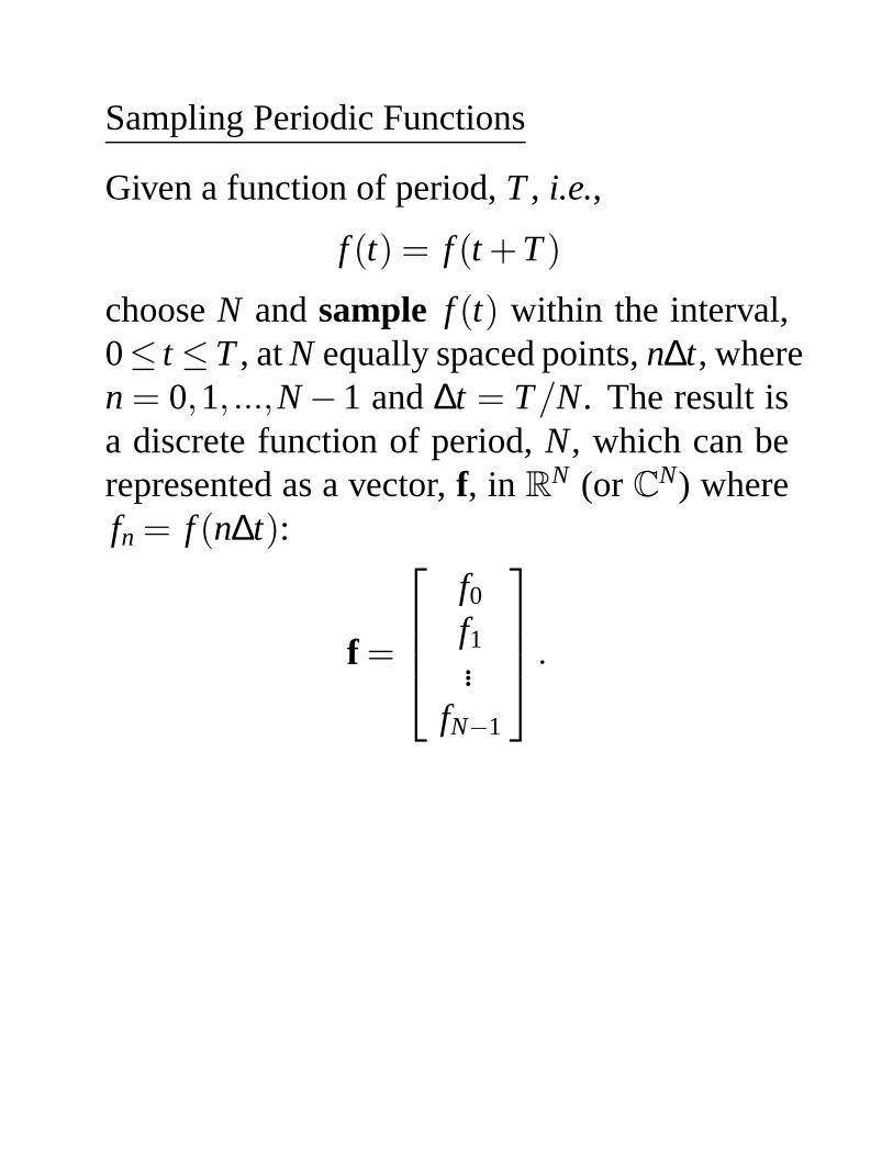
Sampling Periodic Functions

Given a function of period,T , i.e.,

f (t) = f (t +T )

chooseN andsample f (t) within the interval,0≤ t ≤T , atN equally spaced points,n∆t, wheren = 0,1, ...,N −1 and∆t = T/N. The result isa discrete function of period,N, which can berepresented as a vector,f, in R

N (or CN) where

fn = f (n∆t):

f =

f0f1...

fN−1

.

Inner Product of Discrete Periodic Functions

We can define theinner product of two discretefunctions of period,N, as follows:

〈f,g〉 =N−1

∑n=0

f ∗n gn.

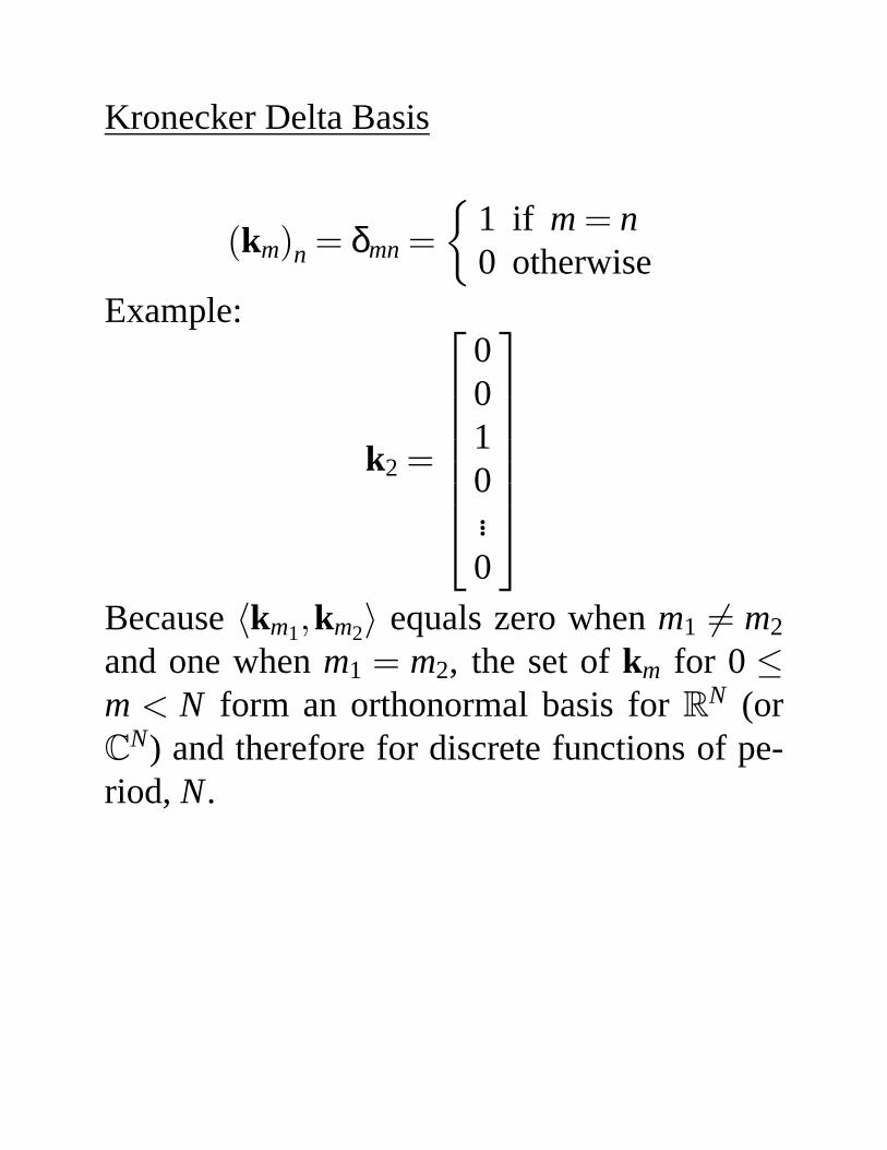
Kronecker Delta Basis

(km)n = δmn =

{

1 if m = n0 otherwise

Example:

k2 =

0010...0

Because〈km1,km2〉 equals zero whenm1 6= m2

and one whenm1 = m2, the set ofkm for 0 ≤m < N form an orthonormal basis forRN (orC

N) and therefore for discrete functions of pe-riod, N.

Sampled Harmonic Signal Basis

A sampled harmonic signal is a discrete func-tion of period,N:

Wn,m =1√N

e j2πm nN

wherem is frequency andn is position. A sam-pled harmonic signal of frequency,m, can berepresented by a vector of lengthN:

wm =

W0,m

W1,m...

WN−1,m

=1√N

e j2πm 0N

e j2πm 1N

...

e j2πm(N−1)N

.

Sampled Harmonic Signal Basis (contd.)

How “long” is a sampled harmonic signal?

‖wm‖ = 〈wm,wm〉12

=

(

N−1

∑n=0

1√N

e− j2πm nN

1√N

e j2πm nN

)12

=

(

N−1

∑n=0

1N

)12

= 1

Sampled Harmonic Signal Basis (contd.)

What is the “angle” between two sampled har-monic signals,wm1 andwm2, whenm1 6= m2?

〈wm1,wm2〉 =1N

N−1

∑n=0

e− j2πm1nN e j2πm2

nN

=1N

N−1

∑n=0

e j2π(m2−m1)nN

=1N

N−1

∑n=0

(

e j2π(m2−m1)N

)n

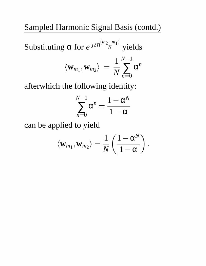
Sampled Harmonic Signal Basis (contd.)

Substitutingα for e j2π(m2−m1)N yields

〈wm1,wm2〉 =1N

N−1

∑n=0

αn

afterwhich the following identity:N−1

∑n=0

αn =1−αN

1−α

can be applied to yield

〈wm1,wm2〉 =1N

(

1−αN

1−α

)

.

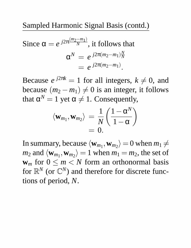
Sampled Harmonic Signal Basis (contd.)

Sinceα = e j2π(m2−m1)N , it follows that

αN = e j2π(m2−m1)NN

= e j2π(m2−m1).

Becausee j2πk = 1 for all integers,k 6= 0, andbecause(m2−m1) 6= 0 is an integer, it followsthatαN = 1 yetα 6= 1. Consequently,

〈wm1,wm2〉 =1N

(

1−αN

1−α

)

= 0.

In summary, because〈wm1,wm2〉= 0 whenm1 6=m2 and〈wm1,wm2〉= 1 whenm1 = m2, the set ofwm for 0 ≤ m < N form an orthonormal basisfor R

N (or CN) and therefore for discrete func-

tions of period,N.

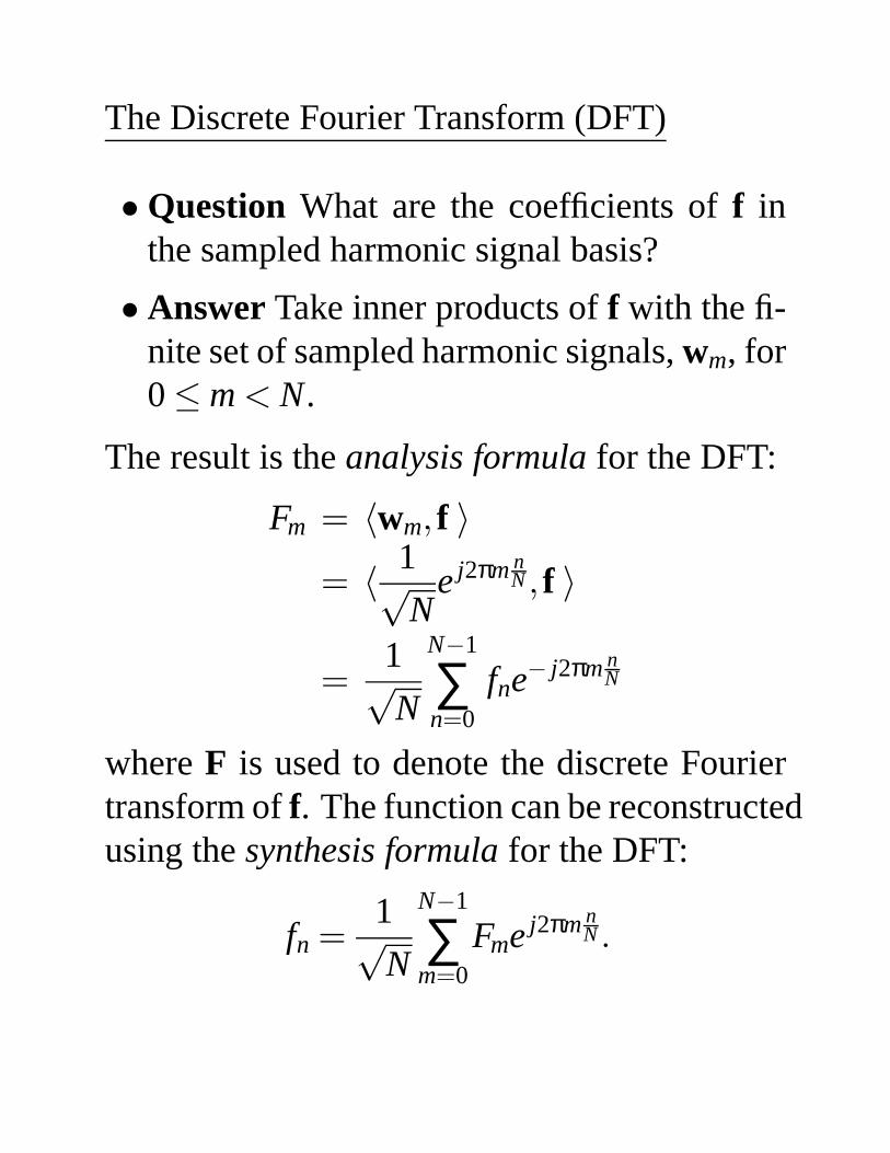
The Discrete Fourier Transform (DFT)

• Question What are the coefficients off inthe sampled harmonic signal basis?

• Answer Take inner products off with the fi-nite set of sampled harmonic signals,wm, for0≤ m < N.

The result is theanalysis formula for the DFT:

Fm = 〈wm, f 〉= 〈 1√

Ne j2πm n

N , f 〉

=1√N

N−1

∑n=0

fne− j2πm nN

whereF is used to denote the discrete Fouriertransform off. The function can be reconstructedusing thesynthesis formula for the DFT:

fn =1√N

N−1

∑m=0

Fme j2πm nN .

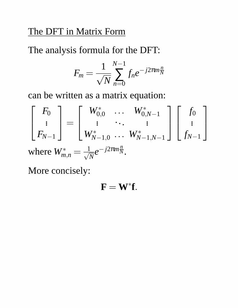
The DFT in Matrix Form

The analysis formula for the DFT:

Fm =1√N

N−1

∑n=0

fne− j2πm nN

can be written as a matrix equation:

F0...

FN−1

=

W ∗0,0 . . . W ∗

0,N−1... . . . ...

W ∗N−1,0 . . . W ∗

N−1,N−1

f0...

fN−1

whereW ∗m,n = 1√

Ne− j2πm n

N .

More concisely:

F = W∗f.

The DFT in Matrix Form (contd.)

The synthesis formula for the DFT:

fn =1√N

N−1

∑m=0

Fme j2πm nN

can also be written as a matrix equation:

f0...

fN−1

=

W0,0 . . . W0,N−1... . . . ...

WN−1,0 . . . WN−1,N−1

F0...

FN−1

whereWm,n = 1√N

e j2πm nN . More concisely:

f = WF.

Note: Because only theproduct of frequency,m, and position,n, appears in the expressionfor a sampled harmonic signal, it follows thatWm,n = Wn,m. ThereforeW = WT. The only dif-ference between the matrices used for the for-ward and inverse DFT’s,i.e., W∗ andW, is con-jugation.

The DFT in Matrix Form (contd.)

A matrix product,y = Ax, can be interpreted intwo different ways.

1. Thei-th component ofy is the inner productof x with the i-th row of A:

y0...

yN−1

=

[

A0,0 . . . A0,N−1]

x0...

xN−1

...

[

AN−1,0 . . . AN−1,N−1]

x0...

xN−1

2. The vector,y, is a linear combination of thecolumns ofA. The i-th column is weightedby xi:

y0...

yN−1

= x0

A0,0...

AN−1,0

+ · · ·+xN−1

A0,N−1...

AN−1,N−1

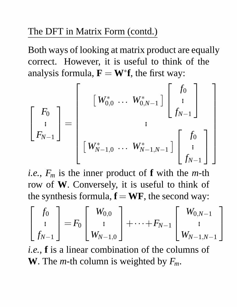
The DFT in Matrix Form (contd.)

Both ways of looking at matrix product are equallycorrect. However, it is useful to think of theanalysis formula,F = W∗f, the first way:

F0...

FN−1

=

[

W ∗0,0 . . . W ∗

0,N−1

]

f0...

fN−1

...

[

W ∗N−1,0 . . . W ∗

N−1,N−1

]

f0...

fN−1

i.e., Fm is the inner product off with the m-throw of W. Conversely, it is useful to think ofthe synthesis formula,f = WF, the second way:

f0...

fN−1

= F0

W0,0...

WN−1,0

+ · · ·+FN−1

W0,N−1...

WN−1,N−1

i.e., f is a linear combination of the columns ofW. Them-th column is weighted byFm.

Matrix Diagonalization

A vector, x, is a right eigenvector whenAxpoints in the same direction asx but is (pos-sibly) of different length:

λx = Ax

A vector,y, is aleft eigenvector whenyTA pointsin the same direction asyT but is (possibly) ofdifferent length:

λyT = yTA

A diagonalizable matrix of rank,N, hasN lin-early independent right eigenvectors

x0, ...,xN−1

andN linearly independent left eigenvectors

y0, ...,yN−1

which share theN eigenvalues

λ0, ...,λN−1.

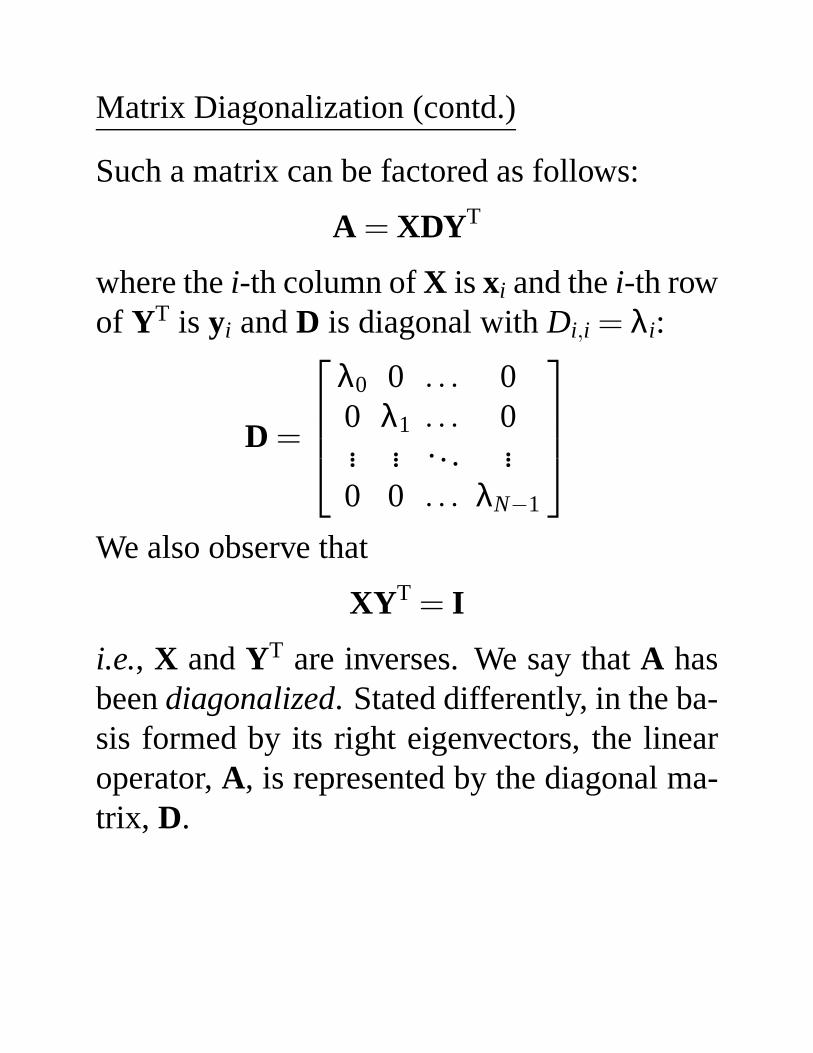
Matrix Diagonalization (contd.)

Such a matrix can be factored as follows:

A = XDYT

where thei-th column ofX is xi and thei-th rowof YT is yi andD is diagonal withDi,i = λi:

D =

λ0 0 . . . 00 λ1 . . . 0... ... .. . ...0 0 . . . λN−1

We also observe that

XYT = I

i.e., X andYT are inverses. We say thatA hasbeendiagonalized. Stated differently, in the ba-sis formed by its right eigenvectors, the linearoperator,A, is represented by the diagonal ma-trix, D.

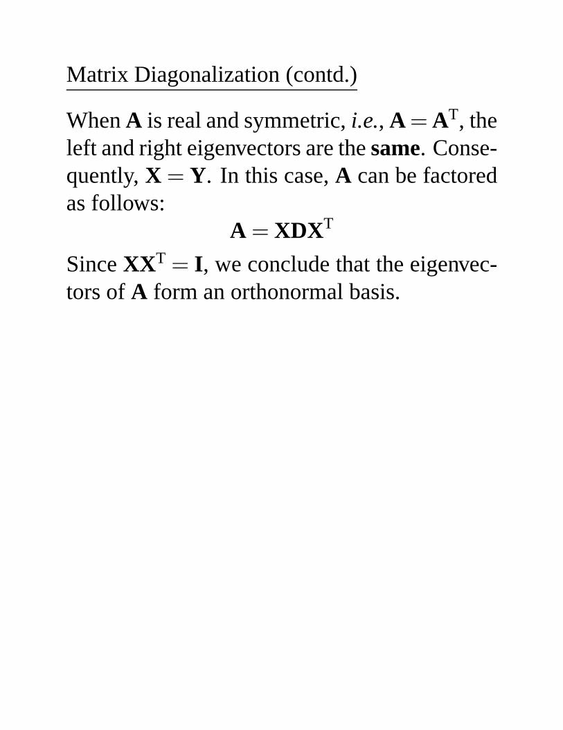
Matrix Diagonalization (contd.)

WhenA is real and symmetric,i.e., A = AT, theleft and right eigenvectors are thesame. Conse-quently,X = Y. In this case,A can be factoredas follows:

A = XDXT

SinceXXT = I, we conclude that the eigenvec-tors ofA form an orthonormal basis.

Matrix Diagonalization (contd.)

The hermitian transpose,AH, of a complex ma-trix, A, is defined to be(A∗)T. WhenA is com-plex and symmetric, the left and right eigenvec-tors arecomplex conjugates. In this case,Acan be factored as follows:

A = XDXH

When the matrix of eigenvectors,X, is also sym-metric,i.e., X = XT, the above simplifies to:

A = XDX∗

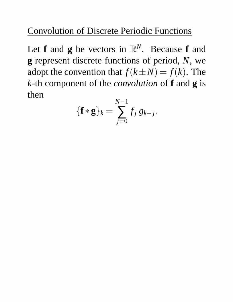
Convolution of Discrete Periodic Functions

Let f and g be vectors inRN. Becausef andg represent discrete functions of period,N, weadopt the convention thatf (k±N) = f (k). Thek-th component of theconvolution of f andg isthen

{f∗g}k =N−1

∑j=0

f j gk− j.

Example of Discrete Periodic Convolution

Calculate{f∗g}k when

g =[

2 1 0 . . . 0 1]T

Sincef∗g = g∗ f and since

{g∗ f}k =N−1

∑j=0

g j fk− j

it follows that

{f∗g}k = g0 fk +g1 fk−1+ · · ·+gN−1 fk−(N−1)

= 2 fk +1 fk−1+1 fk−(N−1)

= fk−1+2 fk +1 fk+1

This operation performs a local weighted aver-aging off.

Circulant Matrices

The convolution formula for discrete periodicfunctions

{f∗g}k =N−1

∑j=0

f jgk− j

can be written as a matrix equation:

f∗g = Cf

whereCk, j = gk− j:

C =

g0 gN−1 gN−2 . . . g1

g1 g0 gN−1 . . . g2

g2 g1 g0 . . . g3... ... ... . .. ...

gN−1 gN−2 gN−3 . . . g0

Matrices likeC are termedcirculant. It is a factthat the right eigenvectors ofall circulant ma-trices are sampled harmonic signals. Further-more, the left eigenvectors ofall circulant ma-trices are sampled conjugated harmonic signals.

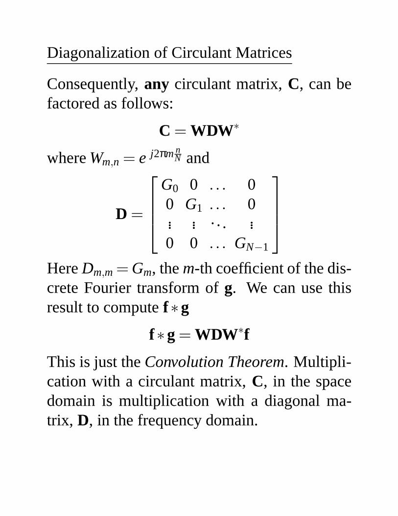
Diagonalization of Circulant Matrices

Consequently,any circulant matrix,C, can befactored as follows:

C = WDW∗

whereWm,n = e j2πm nN and

D =

G0 0 . . . 00 G1 . . . 0... ... . . . ...0 0 . . . GN−1

HereDm,m = Gm, them-th coefficient of the dis-crete Fourier transform ofg. We can use thisresult to computef∗g

f∗g = WDW∗f

This is just theConvolution Theorem. Multipli-cation with a circulant matrix,C, in the spacedomain is multiplication with a diagonal ma-trix, D, in the frequency domain.

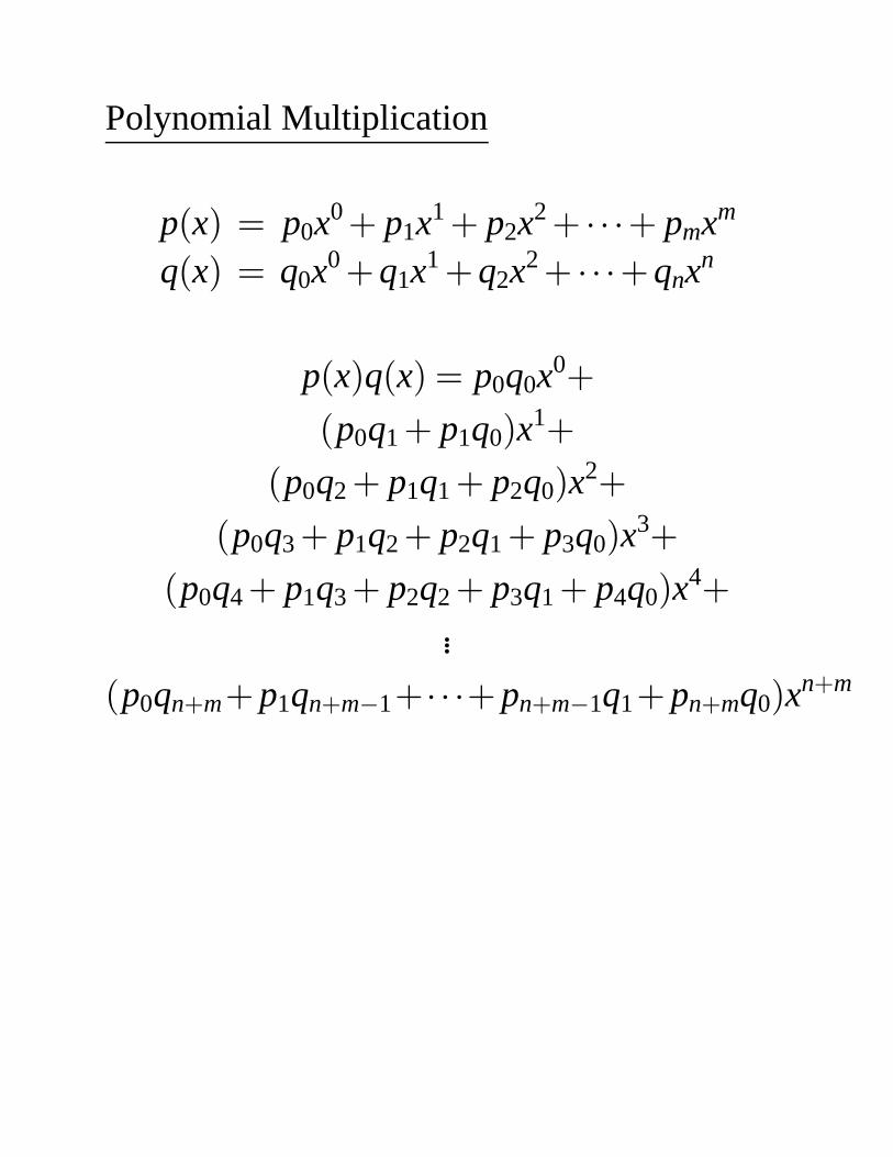
Polynomial Multiplication

p(x) = p0x0+ p1x1+ p2x2+ · · ·+ pmxm

q(x) = q0x0+q1x1+q2x2+ · · ·+qnxn

p(x)q(x) = p0q0x0+

(p0q1+ p1q0)x1+

(p0q2+ p1q1+ p2q0)x2+

(p0q3+ p1q2+ p2q1+ p3q0)x3+

(p0q4+ p1q3+ p2q2+ p3q1+ p4q0)x4+

...

(p0qn+m+ p1qn+m−1+ · · ·+ pn+m−1q1+ pn+mq0)xn+m

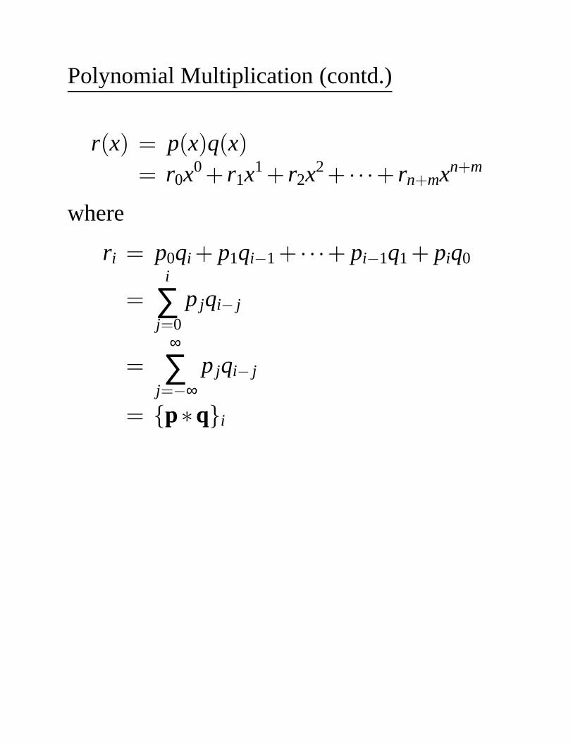
Polynomial Multiplication (contd.)

r(x) = p(x)q(x)= r0x0+ r1x1+ r2x2+ · · ·+ rn+mxn+m

where

ri = p0qi + p1qi−1+ · · ·+ pi−1q1+ piq0

=i

∑j=0

p jqi− j

=∞

∑j=−∞

p jqi− j

= {p∗q}i