The Distribution of Environmental Damages∗

Solomon Hsiang,1 Paulina Oliva,2 and Reed Walker3

1University of California, Berkeley, and NBER; e-mail: shsiang@berkeley.edu

2University of California, Irvine, and NBER; e-mail: bolivava@uci.edu

3University of California, Berkeley, and NBER; e-mail: rwalker@berkeley.edu

Abstract

Most regulations designed to reduce environmental externalities impose costs on individuals and

firms. An active body of research has explored how these costs are disproportionately born by

different sectors of the economy and/or across different groups of individuals. However, much

less is known about the distributional characteristics of the environmental benefits created by

these policies, or conversely, the differences in environmental damages associated with existing

environmental externalities. We review this burgeoning literature and develop a simple and general

framework for focusing future empirical investigations. We apply our framework to findings related

to the economic impact of air pollution, deforestation, and climate, highlighting important areas

for future research. A recurring challenge to understanding distributional effects of environmental

damages is distinguishing between cases where (i) populations are exposed to different levels or

changes in an environmental good, and (ii) where an incremental change in the environment may

have very different implications for some populations. In the latter case, it is often difficult to

empirically identify the underlying sources of heterogeneity in marginal damages, as damages may

stem from either non-linear and/or heterogeneous damage functions. Nonetheless, understanding

the determinants of heterogeneity in environmental benefits and damages is crucial for welfare

analysis and policy design.

∗We would like to thank Hannah Druckenmiller, Eyal Frank, Don Fullerton, Teevrat Garg, Peiley Lau, and JosephShapiro for helpful comments. Andres Gonzalez and Eva Lyubich generously provided research assistance for this project.All errors are our own. This version: July 20, 2017

1

Economists have long understood that the benefits to environmental regulations are unlikely to be

evenly distributed across individuals within a given population. As early as the 1980’s, researchers and

policy makers became specifically concerned that lower income populations might be disproportionately

exposed to and impacted by environmental externalities, such as air and water pollution, leading rise

to the notion of “environmental justice” (see e.g., US GAO (1983) and United Church of Christ

(1987)). We review and discuss what is understood about the distribution of environmental benefits

(or conversely, damages), while highlighting how policies designed to mitigate environmental damages

alter this distribution. An established literature has long considered how different environmental policy

instruments produce winners and losers by imposing different regulatory costs on individuals (Baumol

and Oates, 1988; Parry et al., 2006; Fullerton, 2017), but because a large share of environmental

benefits correspond to non-market outcomes, such as health impacts, they are often more difficult to

trace than the direct pecuniary costs of the regulation itself. Due to this difficulty, it is not generally

known if most environmental policies are, on net, progressive, regressive, or have no distributional

effects (Fullerton, 2011; Parry et al., 2006; Bento, 2013).

In our exploration of what is known empirically about the distribution of environmental benefits,

we organize our discussion using a general framework that highlights the underlying sources of hetero-

geneity in these benefits, while also discussing what these underlying sources may suggest for welfare

analysis and/or policy-making. Our framework is intentionally simple, focusing on the structure of

damage functions and the key challenges that we see in the literature: separating out heterogeneity

in damages that originate from differences in environmental exposure, differences in damage functions

across individuals, and/or non-linearities within a single damage function. Then, to demonstrate its

generality, we examine three core areas of study in empirical environmental economics—pollution, de-

forestation, and climate change—through this lens. These three topic areas are generally considered

at three very different spatial scales and are currently studied with differing levels of sophistication.

However, all three can be placed in our common framework, demonstrating its broad applicability.

An environmental policy may generate an uneven distribution of benefits across populations if (i)

the policy delivers uneven quantities of an environmental good and/or (ii) the benefits from an incre-

mental improvement in the environmental good differ across populations. The first case is largely a

question of policy design and the physical relationships that govern the distribution of the environmen-

tal good—these factors sound straightforward, but challenges associated with measurement of unevenly

distributed environmental goods are often substantial. At the heart of second case lie questions about

2

the underlying sources of heterogeneity in benefits/damages associated with an incremental change in

the environment. These differences may stem from uneven baseline levels of exposure combined with

non-linear dose-response functions. These differences may also arise because dose-response functions

differ across populations (e.g., due to differences in the underlying stock of health and/or differences

in defensive investments). Individuals might also have differing preferences over environmental goods

that potentially alter how dose-response relationships map into individual well-being or welfare. In

cases where environmental benefits are thought to be distributed unevenly, identifying which of these

mechanisms drives the unequal impact is key to understanding how distributional effects should be

valued and possibly ameliorated through policy.

To date, empirically identifying the causes of heterogeneous marginal damages has had only modest

success. Econometrically, the core difficulty is that observable predictors of heterogeneity in dose-

response functions (e.g., income) are not randomly assigned. Thus, empirically determining what

drives any observed heterogeneity in a dose-response, whether it is income or one of many other

factors correlated with income (e.g., defensive investments, health stock, or baseline exposure), is

difficult. Nonetheless, solving this empirical problem is important because the source of heterogeneity

matters when translating estimates of dose-response functions into welfare metrics or marginal damages

(Grossman, 1972; Courant and Porter, 1981; Bartik, 1988). This identification challenge plagues many

environmental policy contexts and will likely require creative research designs to solve.

Structure of the problem

We believe it useful to break down the central conceptual components associated with environmental

externalities and the ways that they are differentially manifested among segments of the population.

Broadly speaking, heterogeneity in damages from externalities can stem from differences in exposure

and/or differences in marginal damages, conditional on exposure.

An environmental externality (described here as a “damage,” i.e. negative benefit, for simplicity)

is a cost that may be written as a general function of two components: the level of exposure to

environmental conditions e and a vector of attributes x that may influence how exposure affects

measures of economic well-being:

Damage = f(e,x)

where f(.) is a function that translates exposure and individual attributes into damages in welfare

3

terms, such as a willingness-to-pay. We define exposure e as the state of the environment at an

arbitrary point in time and space. For example, exposure refers to the physical amount of air pollutant,

deforestation, and/or temperature that a location experiences at a moment in time. In most cases,

exposure is measured in physical units that describe some dimension of the environmental system in

question, such as “parts per million” for air pollution, “share of land cleared of trees” for ecosystem

services, or “maximum daily temperature” for climate.1 We note that the vector of attributes x

that translate exposure into damages are potential underlying sources of vulnerability, i.e. factors

that may make individuals more vulnerable to exposure by making it costlier for them to experience.

Vulnerability, could depend on a wide range of factors that differ across individuals–such as baseline

health, avoidance behavior, or defensive investments. Many of these factors could be considered

forms of human-made capital and thus their influence on f(.) may be understood to indicate some

substitutability or complementarity with the form of natural capital described by e (Solow, 2012).

Thus, in this framework, exposure is only converted into terms of economic cost through a function

that describes the vulnerability of an individual or population, i.e. how exposure (treatments) translate

into costs (treatment effects). By way of an example using air pollution–exposure refers to the amount

of the harmful air pollutant in the atmosphere, whereas vulnerability, which depends on x, tells us

how that concentration will ultimately translate into changes in individual welfare.

A policy change may alter the exposure of individual i from its pre-policy state ei to a post-policy

state ei + ∆ei, producing a benefit equal to the change in damages

∆Damagei = f(ei + ∆ei,xi)− f(ei,xi)

making it clear that the policy may have distributional consequences for two possible reasons. First,

if the change in environmental exposure ∆ei differs substantially across individuals, then the change

in damages will also likely differ, regardless of what the initial allocation of ei is or the structure of

f(.). Second, even if the change in exposure is relatively uniform across individuals (perhaps because

1Some existing frameworks discussing air pollution damages distinguish between “ambient concentration” (the mea-sured parts per million in the atmosphere), “dose” (how much did an individual ingest), “response” (the relationshipbetween the dose and health outcomes), and “valuation” (the welfare costs of the health response). In our framework ecorresponds to ambient concentration (which is affected by policy), and f(.) translates e into welfare terms. Differencesin “dose”, “response”, and “valuation”—as they are used in that literature—are manifested through the different waysthat the vector of attributes x mediate the translation of e into damage through f(.).

4

ff

e1 e2 e1 e2

f(e1,x1)

f(e2,x2)

f(e)

e e

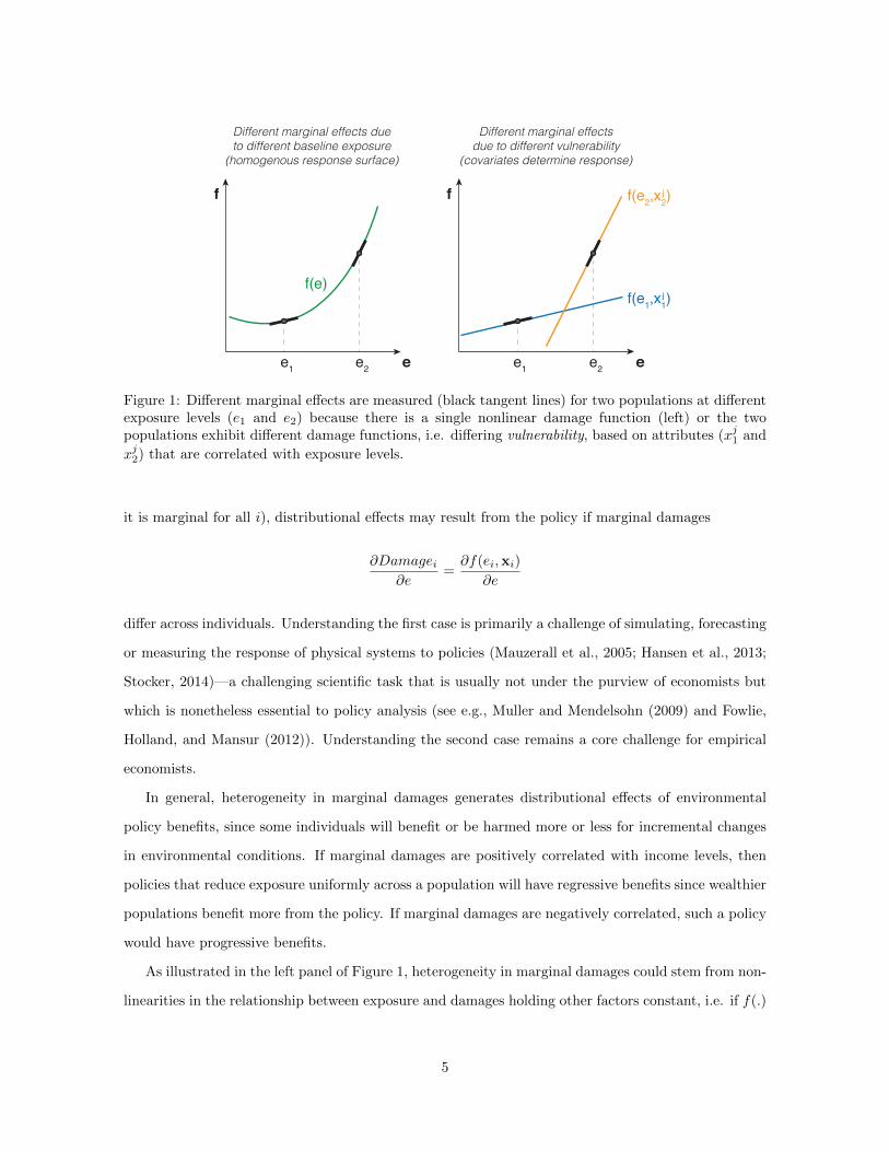
Different marginal effects dueto different baseline exposure

(homogenous response surface)

Different marginal effectsdue to different vulnerability

(covariates determine response)

j

j

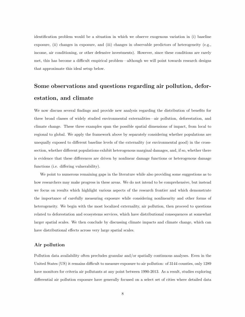
Figure 1: Different marginal effects are measured (black tangent lines) for two populations at differentexposure levels (e1 and e2) because there is a single nonlinear damage function (left) or the twopopulations exhibit different damage functions, i.e. differing vulnerability, based on attributes (xj

1 and

xj2) that are correlated with exposure levels.

it is marginal for all i), distributional effects may result from the policy if marginal damages

∂Damagei∂e

=∂f(ei,xi)

∂e

differ across individuals. Understanding the first case is primarily a challenge of simulating, forecasting

or measuring the response of physical systems to policies (Mauzerall et al., 2005; Hansen et al., 2013;

Stocker, 2014)—a challenging scientific task that is usually not under the purview of economists but

which is nonetheless essential to policy analysis (see e.g., Muller and Mendelsohn (2009) and Fowlie,

Holland, and Mansur (2012)). Understanding the second case remains a core challenge for empirical

economists.

In general, heterogeneity in marginal damages generates distributional effects of environmental

policy benefits, since some individuals will benefit or be harmed more or less for incremental changes

in environmental conditions. If marginal damages are positively correlated with income levels, then

policies that reduce exposure uniformly across a population will have regressive benefits since wealthier

populations benefit more from the policy. If marginal damages are negatively correlated, such a policy

would have progressive benefits.

As illustrated in the left panel of Figure 1, heterogeneity in marginal damages could stem from non-

linearities in the relationship between exposure and damages holding other factors constant, i.e. if f(.)

5

is non-linear with respect to e then two individuals facing different baseline levels ei will experience

different marginal damages, even if they are identical in terms of all other factors that determine

vulnerability:

∂2Damage

∂e2=

∂2f(e,x)

∂e26= 0

Alternatively—or in addition—heterogeneity in marginal damages may stem from heterogeneity in an

underlying attribute, here the jth element in x, that controls how exposure translates into damages,

i.e. xj may affect vulnerability:

∂Damage

∂e∂xj=

∂2f(e,x)

∂e∂xj6= 0

illustrated in the right panel of Figure 1.

Identifying cases where marginal damages are heterogenous is usually sufficient to conclude that

environmental policy may have uneven benefits. However, designing efficient environmental policy

and/or addressing any resulting distributional effects may require understanding the source of this

heterogeneity. Do they differ because baseline exposure differs or because vulnerability differs? For

example, does warming a country’s climate harm poor countries more because they have greater vul-

nerability to climate (Dell, Jones, and Olken, 2012) or because poor countries tend to be hotter and

damages are nonlinear in temperature (Burke, Hsiang, and Miguel, 2015)? These two different ex-

planations for the same empirical observation generate highly divergent forecasts for global economic

development in a scenario where countries both warm and become wealthier simultaneously, highlight-

ing the importance of understanding underlying sources for these types of heterogeneity.

In cases where heterogeneous marginal damages generate distributional impacts of environmental

policies, empirically decomposing the sources of heterogeneity is important for understanding the social

costs of environmental externalities and for considering potential policy interventions. Moreover, the

extent to which we can extrapolate damages measured in one population to others depends on our

understanding of how heterogeneity in damages is manifested.

Two practical empirical considerations

Beyond standard econometric concerns regarding causal inference and the identification of marginal

effects (see e.g., Angrist and Pischke (2010)), two particularly important and general measurement

issues arise when trying to understand the distributional benefits of environmental services and/or

policy.

6

First, many policies or exogenous events will change environmental exposure in different areas

by different quantities. Measuring these heterogenous changes in exposure is difficult because data

measuring exposure is often imperfect and/or incomplete. Moreover, mismeasurement of exposure can

exacerbate the challenges associated with understanding the nature and magnitude of heterogeneous

marginal damages. Since marginal damages are measured in cost per unit of exposure, comparing

marginal damages across contexts requires that marginal losses are identified relative to an objective

and physically consistent measure of exposure. This can present a challenge when comparing marginal

damages if the spatial scales of measurement for exposure vary substantially across studies (e.g.,

examining pixels vs. countries) or if exposure is encoded using context-specific and/or non-physical

units. For example, it is often econometrically convenient to transform environmental exposure into

a binary variable, such as encoding observations with high levels of deforestation or tropical cyclone

strikes as a dummy variable equal to one. However, such an approach may not allow meaningful

comparisons of marginal damages across contexts since variation in physical exposure experienced

by populations may differ dramatically between observations that are all encoded using a common

“treated” dummy.

The second measurement challenge stems from the difficulty at empirically distinguishing between

the two cases in Figure 1, even when levels of environmental exposure are well measured and heteroge-

nous marginal effects are convincingly estimated. This identification problem stems primarily from the

fact that researchers often observe only a single tangency on a dose-response function, rather than the

entire function for different sub-groups. Thus, when researchers observe differences in marginal effects,

it may be hard to identify if these differences stem from different points on the same, non-linear dose

response function or points on different dose-response functions. For example, baseline levels of envi-

ronmental exposure (ei) are rarely randomly assigned, and they are often correlated with covariates

xi. For this reason it is often difficult to demonstrate that there exists a homogenous and nonlinear

response function (left panel of Figure 1). Moreover, even if levels of environmental treatment e are

randomly assigned, the covariates x are usually not, making it difficult to pin down which elements in

x cause differences between dose-response functions. As highlighted above, understanding the reasons

for which dose-response functions differ is crucial both for valuing damages as well as understanding

how damages may be mitigated through policy. For example, if we observe different dose-response

functions for different income groups, these differences in responses may not be driven by income but

instead some other correlated unobservable (e.g., baseline health stock). The ideal solution to this

7

identification problem would be a situation in which we observe exogenous variation in (i) baseline

exposure, (ii) changes in exposure, and (iii) changes in observable predictors of heterogeneity (e.g.,

income, air conditioning, or other defensive investments). However, since these conditions are rarely

met, this has become a difficult empirical problem—although we will point towards research designs

that approximate this ideal setup below.

Some observations and questions regarding air pollution, defor-

estation, and climate

We now discuss several findings and provide new analysis regarding the distribution of benefits for

three broad classes of widely studied environmental externalities—air pollution, deforestation, and

climate change. These three examples span the possible spatial dimensions of impact, from local to

regional to global. We apply the framework above by separately considering whether populations are

unequally exposed to different baseline levels of the externality (or environmental good) in the cross-

section, whether different populations exhibit heterogenous marginal damages, and, if so, whether there

is evidence that these differences are driven by nonlinear damage functions or heterogenous damage

functions (i.e. differing vulnerability).

We point to numerous remaining gaps in the literature while also providing some suggestions as to

how researchers may make progress in these areas. We do not intend to be comprehensive, but instead

we focus on results which highlight various aspects of the research frontier and which demonstrate

the importance of carefully measuring exposure while considering nonlinearity and other forms of

heterogeneity. We begin with the most localized externality, air pollution, then proceed to questions

related to deforestation and ecosystems services, which have distributional consequences at somewhat

larger spatial scales. We then conclude by discussing climate impacts and climate change, which can

have distributional effects across very large spatial scales.

Air pollution

Pollution data availability often precludes granular and/or spatially continuous analyses. Even in the

United States (US) it remains difficult to measure exposure to air pollution: of 3144 counties, only 1289

have monitors for criteria air pollutants at any point between 1990-2013. As a result, studies exploring

differential air pollution exposure have generally focused on a select set of cities where detailed data

8

are available (e.g., Depro, Timmins, and O’Neil (2015)) or communities that are sufficiently proximate

to a facility that emits toxic air pollutants such that certain levels of exposure can reasonably be

assumed (e.g., Been and Gupta (1997); Banzhaf and Walsh (2008)). Recent advances in measurement

and modeling may address some of these longstanding data challenges. For example, researchers have

recently created ambient pollution data products for the US over time by merging fixed-site pollution

monitors, satellite- derived NO2 estimates, and GIS-derived land-use data (see e.g., Novotny et al.

(2011)). These granular and spatially continuous air pollution measures may afford researchers new

possibilities, such as the ability to connect pollution exposure with high resolution demographic data.

We use the data from Novotny et al. (2011) to explore differences in pollution exposure across US

Census Block-Groups.2

Some cross-sectional patterns in air-pollution exposure

In the US, cross-sectional differences in air pollution exposure are ubiquituous. A range of empirical

papers that date back to the 1970’s documented that low income individuals disproportionately live in

areas with higher environmental risk (Freeman, 1974; Harrison and Rubinfeld, 1978), closer to toxic

facilities (Brooks and Sethi, 1997) and Superfund hazardous waste sites (Hamilton, 1993; Currie, 2011),

and/or power plants (Davis, 2011). However, the evidence on differences in air pollution exposure has

been relatively indirect and piecemeal due to the measurement challenges described above. We shed

some additional light on differential pollution exposure by using newly available, high-resolution data

on ambient NO2 levels in the US (Novotny et al., 2011). We link these gridded pollution data to

the 2010 Decennial Census at the Block-Group level and explore relationships between income and

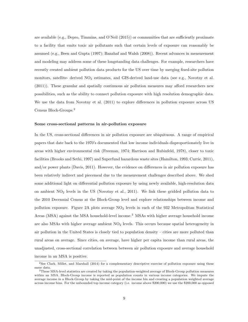
pollution exposure. Figure 2A plots average NO2 levels in each of the 932 Metropolitan Statistical

Areas (MSA) against the MSA household-level income.3 MSAs with higher average household income

are also MSAs with higher average ambient NO2 levels. This occurs because spatial heterogeneity in

air pollution in the United States is closely tied to population density – cities are more polluted than

rural areas on average. Since cities, on average, have higher per capita income than rural areas, the

unadjusted, cross-sectional correlation between between air pollution exposure and average household

income in an MSA is positive.

2See Clark, Millet, and Marshall (2014) for a complementary descriptive exercise of pollution exposure using thesesame data.

3These MSA-level statistics are created by taking the population-weighted average of Block-Group pollution measureswithin an MSA. Block-Group income is reported as population counts in various income categories. We impute theaverage income in a Block-Group by taking the mid-point of the income bin and creating a population weighted averageacross income bins. For the unbounded top income category (i.e. income above $200,000) we use the $200,000 as opposed

9

0

5

10

15

20Am

bien

t NO

2 (p

pb)

40 60 80 100MSA Average Household Income

(thousands of dollars)

1204

6

8

10

12

14

Ambi

ent N

O2

(ppb

)

0 20 40 60 80 100

Within-MSA Income Percentile of Block-Group

8

9

10

11

12

Ambi

ent N

O2

(ppb

)

0 20 40 60 80 100

Block-Group National Income Percentile

A B C

Figure 2: This figure presents three panels relating 2010 Census Block-Group NO2 exposures tohousehold income. Panel A plots the relationship between average MSA NO2 levels and MSA-levelhousehold income. Panel B plots the relationship between average NO2 levels and the Block-Groupnational income percentiles. Panel C plots the within-MSA relationship between NO2 levels and MSABlock-Group income percentiles. See text for details. Source: Novotny et al. (2011) and 2010 DecennialCensus.

However, MSA-level aggregates obscure a tremendous amount of household-level variation in expo-

sure levels. Figure 2B plots the relationship between Block-Group household average income percentiles

(based on the national Block-Group income distribution) and average NO2 levels in the Block-Group

income percentile. We see that, on average, there is a U-shaped relationship between income and

exposure, with low and high income percentile Block-Groups in the United States disproportionately

exposed to high ambient pollution levels relative to Block-Group income percentiles towards the center

of the national income distribution. This finding can be partially reconciled with Figure 2A by noting

that some of the wealthiest and poorest Block-Groups are both located in large MSAs – MSAs that,

on average, have higher pollution levels.

Importantly, national cross-sectional patterns differ from patterns of environmental exposures

within a given MSA. In order to look at the average within-MSA relationship between income and

exposure, we compute the percentile of average income for each Block-Group separately within each

MSA. We then compute the average exposure level for each percentile and plot this relationship in

Figure 2C. The within-MSA correlation appears to be opposite of what is observed across MSAs:

the average relationship between pollution exposure and income within MSAs is strictly negative, with

poorer areas in each MSA characterized by higher levels of ambient pollution than richer areas. Similar

disparities exist for other monitored criteria air pollutants.

to an undefined mid-point.

10

An area of interest for future inquiry is how these cross-sectional relationships change over time.

One striking fact that emerges from extending our analysis above is that the gap in ambient air

pollution levels between relatively affluent and less affluent households may be closing. Repeating the

analysis in Figure 2C using data from 2000 suggests that households in low-income areas of an MSA

have seen much larger recent improvements in air quality relative to nearby households in wealthier

Block-Groups. While more research is needed to understand this pattern, such convergence in outcomes

seems likely to be driven by the targeted nature of Clean Air Act (CAA) regulations. For example, the

CAA abates pollution in areas of a city/county where pollution levels are highest, leading to relatively

larger environmental benefits for poorer Block-Groups within an MSA (Bento, Freedman, and Lang,

2015).

Identifying heterogeneous marginal effects of air pollution

A persistent negative correlation between air pollution exposure and income per capita in the cross-

section suggests that the air pollution burden is not borne equally across the population. However,

disproportionate exposure need not necessarily mean disproportionate differences in damages or well-

being. For example, if air quality is a normal good, then lower-income households may choose to

consume less of the environmental good in exchange for cheaper housing. In addition, individuals who

choose to live in more polluted areas may have invested in measures to protect themselves against

disproportionate exposure such as the purchasing of air filters or buying bottled water. To understand

whether differences in exposure correspond to differences in well-being, we need information on the

marginal damage associated with a given level of exposure, an area where researchers have made

substantial progress over the past 15 years. We discuss a few of these studies, focusing on work that

attempts to address what we believe are the first order statistical challenges in this area – in particular

concerns pertaining to bias stemming from omitted variables.

Starting with the pioneering work by Chay and Greenstone (2003a,b) researchers have exploited

research designs appropriate for causal inference to deliver well-identified estimates of the average

effect of a one unit change in air pollution exposure on health and welfare. These approaches allow

researchers to begin exploring heterogeneity in the causal effects of pollution exposure, possibly caused

by differences in observable characteristics of the population and/or non-linearities in the dose-response

function. For example, Chay and Greenstone (2003b) explore heterogeneity in the infant-health dose-

response function across different races – finding that African Americans have more negative health

11

responses to increases in air pollution than do Whites in their sample. Similarly, Currie and Walker

(2011) observe that health effects of traffic related air pollution are larger for African Americans

relative to Whites. Jayachandran (2009) observes a striking difference in the mortality effects of

pollution between richer and poorer places. Arceo, Hanna, and Oliva (2016) find that the mortality

effects of carbon monoxide in Mexico are almost ten-times the effects found in similar estimates for US

populations (Currie and Neidell, 2005). Schlenker and Walker (2015) find those over the age of 65 are

more vulnerable to marginal changes in carbon monoxide exposure (CO) and, similarly, Deschenes,

Greenstone, and Shapiro (Forthcoming) observe significantly larger responses in elderly mortality to

variation in NOx exposure.

The evidence above suggests that air pollution dose-response functions are heterogeneous across

different subgroups of the population. However, there is much less evidence that these differences

in health-related dose-response functions translate into differences in marginal damages or welfare.

Moreover, attributing observable heterogeneity in a dose-response function and/or marginal damages

to a single explanatory factor is challenging since the underlying explanatory factor may be endogenous

or correlated with important unobservable factors. For example, heterogeneity in pollution-induced

mortality by income could arise because low-income individuals are more vulnerable to air pollution

exposure–perhaps because of low baseline health or limited protective investments–or because they

disproportionately live in areas with higher levels of exposure and the dose-response function is non-

linear. If the dose-response function is non-linear and rich and poor communities have unequal levels

of baseline pollution exposure, then marginal effects will differ for the same dose-response function (i.e.

left panel of Figure 1). Alternatively, or in addition, low income individuals may have lower levels of

baseline health for which a one unit increase in air pollution can lead to more severe mortality effects

(i.e. right panel of Figure 1). Few, if any, analyses explore the causes of treatment effect heterogeneity

by exploiting exogenous variation in potential mediating factors (including baseline exposure), and

this seems like a clear direction for future research. As discussed above, these distinctions matter for

understanding the efficacy of any policy responses designed to alleviate any of the observed disparities.

Some policy discussions concerning air pollution

Even with well-identified average dose-response functions, understanding the distributional benefits

of air pollution policy remains challenging. One difficulty stems from the fact that the underlying

source of heterogeneity in dose-response function matters for welfare and incidence of a policy. For

12

example, if some individuals invest in defensive behavior, which alters the dose-response relationship

for this sub-population, then the costs of these investments should be included in estimates of the

marginal damage (Grossman, 1972; Courant and Porter, 1981; Bartik, 1988). The absence of random

variation in the observable predictors of treatment effect heterogeneity make it difficult to pinpoint the

precise source of heterogeneity – a crucial ingredient for welfare analysis. Future researchers therefore

must develop creative research designs to understand the distributional benefits of environmental

policies. For example, did the CAA disproportionately improve the plight of some groups of individuals

relative to others because it targeted locations with high baseline exposure levels? The law leads to

substantial spatial heterogeneity in the way in which it impacts air quality around the United States,

begging the question as to how these changes map to different subgroups of the population and the

corresponding benefits. Moreover, it might be the case that improvements in environmental quality

affect market prices and/or wages in ways that could differentially impact household welfare, and

understanding the distributional impacts of environmental policy requires researchers to grapple with

these general equilibrium issues. For example, Bento, Freedman, and Lang (2015) show that lower-

income homeowners tended to enjoy the greatest benefits from the 1990 CAAA, as these were the

homeowners located in areas that experienced the largest improvements in air quality. Based on house

price appreciation, households in the lowest quintile of the income distribution received annual benefits

from the program equal to 0.3% of their income on average during the 1990s, over twice as much as

those in the highest quintile. However, higher-income households are more likely to be homeowners,

and thus may be more likely to reap the benefits of any capitalization of environmental improvements

into property values (Grainger, 2012). While the literature on the distributional benefits of the Clean

Air Act tells us that air quality has improved disproportionately in low income areas, it says relatively

little about how low income consumers differentially value the same marginal improvement in air

quality. More generally, understanding how willingness to pay for non-market amenities varies with

income is a fundamental question for discussing incidence of environmental benefits, but the existing

evidence is weak and indirect – much of the observed heterogeneity observed in WTP by income may

be driven by other observable or unobservable factors that are simply correlated with income.

Deforestation and associated ecosystem services

Ecosystem services encompass a broad number of ways in which ecosystems benefit society. We limit

our discussion to those services that accrue to non-owners of the resource; i.e. those that are not

13

completely internalized by the owners’ use of the resource. Timber and non-timber products from

a single-owner forest are not considered externalities; while pest control, soil fertility, and watershed

services may constitute externalities when accrued to non-forest owners. This distinction is important,

as the existence of public benefits of ecosystems is what motivates many policy interventions, both

from an efficiency standpoint and from any approach that values distributional effects.

Even within this narrower definition of ecosystem services, the measurement of their benefits faces

a unique challenge – namely, the diverse nature and geographic scope of all externalities that fall in

this category. Ecosystem services as externalities emerge from a wide array of human interactions with

nature. For example, humans rely on forests for watershed services, erosion prevention, soil fertility,

local climate, global climate, preservation of biodiversity, recreation, etc. Other natural resources,

such as water bodies, coral reefs, and wetlands, provide an equally diverse set of services. For our

discussion of the distribution of benefits stemming from ecosystems we will focus on forests, as they

are the source of numerous ecosystem services and their location, health, and evolution is relatively

well documented. Greater availability of forest data has also facilitated research on this particular

system, and thus a wider literature sheds light on patterns and sources of heterogeneity in ecosystem

services from forests. Nevertheless, many of the conceptual and empirical issues that we highlight are

common to ecosystem services that are not related to forests.

The two main challenges associated with studying ecosystem services are measurement and valua-

tion. Many of the services that forests provide, such as soil fertility, local biodiversity, erosion protection

are often difficult to track and measure in a comprehensive way. Moreover, even if researchers could

measure these services well, it is often difficult to estimate or measure how forest cover affects these

services. Forests may affect other ecosystems in a variety of ways and at very different geographic

scales. For example, while exposure to soil fertility benefits might be limited to a few meters from a

forest, local biodiversity services (e.g., pest control) could extend up to 0.5-10 km from the forest’s

edge (Bianchi, Goedhart, and Baveco, 2008; Karp et al., 2013), and watershed services may extend

to entire river basins, which can span several countries (Myers, 1997). Even if researchers are able to

estimate the complex relationships between forest cover and other ecosystem services, it is exceedingly

difficult to understand how these services are valued. There is rarely an observed market price for

these services, and some of the services provided may benefit individuals thousands of miles away

through recreational uses and/or “existence value”. Researchers have used a wide variety of empirical

methods to try to monetize these benefits, ranging from stated-preference, survey based methods to

14

other revealed-preference methods, such as hedonic valuation. We discuss this literature in more detail

below.

Some cross-sectional patterns in deforestation exposure

Before turning to the existing literature, we use data from the World Bank Indicators to provide some

descriptive statistics on the within and between country relationships between exposure to forest cover

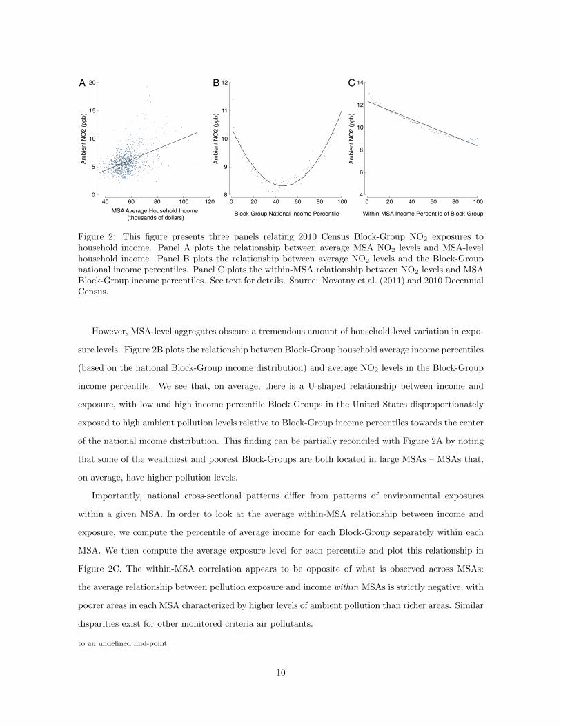
and various measures of socioeconomic status.4 Figure 3A plots the cross-country relationship between

forest cover (as a percentage of total land) and the logarithm of GDP per capita. This figure points to

tremendous variation in forest endowments across both rich and poor countries. Thus, if the marginal

benefits of additional forest preservation were similar across countries, policies aimed at preserving

current forest stocks across all countries would have neutral distributional effects.

Country averages are a relatively crude measure of exposure to forest ecosystem services which

might mask important within country heterogeneity. However, sub-national data on exposure to

forest cover linked to demographic characteristics is not available for many countries. The World

Bank Indicators do provide information on the rural poor as a percentage of overall population, and

since forests are by definition rural, we can use this data to crudely explore whether relatively poor

populations systematically have higher or lower exposure to forest ecosystem services. Figure 3B

shows no systematic relationship between the share of rural poor and forest cover. Thus, even when

conditioning on the relative size of population that would be most likely exposed to ecosystem services

(i.e., rural populations), exposure to forest cover stocks appears uniform across countries. This coarse

proxy for poverty potentially near forests could mask important differences in actual forest endowments

across income groups within a country, especially for the extreme poor. Some of these within-country

differences have been documented by the literature. For example, 84% of tribal ethnic minorities in

India live in forested areas (Mehta and Shah, 2003), and large overlaps between severe poverty and

forests exist within China and Vietnam (Li and Veeck, 1999; Sunderlin and Huynh, 2005).

While forest stocks play a role in the generation of ecosystem services, forest policies operate on

the margin of these stocks by altering flows, partially determining if stocks are increasing or decreasing

at a moment in time. Figures 3C and 3D plot the relationship between forest cover changes between

4The cross-country relationship between income and deforestation has received substantial attention from studiestesting for the existence of an “Environmental Kuznets Curve” (EKC) – the idea that exposure to deforestation is higherfor economies in transition undergoing rapid industrialization (Cropper and Griffiths, 1994; Van and Azomahou, 2007).Over time, as countries become wealthier, they tend to increase the area of land under protection (Frank and Schlenker,2016). Our goal here is not to revisit this literature but instead document how forest exposure may differ across differentsub-groups and what that may mean for the regressivity/progressivity of various land use policies.

15

ABWAFG

AGO

ALB

ARB AREARM

ATGAUS

AUT

AZEBDI

BEL

BEN

BFABGD

BGR

BHR

BHSBIH BLR

BLZ

BMU

BOLBRA

BRB

BRNBTN

BWA

CAF CANCEB CHECHLCHN

CIVCMR

COG

COL

COM CPV

CRI

CSS

CUB

CYM

CYP

CZEDEU

DJI

DMA

DNK

DOM

DZA

EAPEAR EAS

ECAECS

ECU

EGY

EMU

ERI

ESP

EST

ETH

EUU

FCS

FIN

FJI

FRA

FSM GAB

GBR

GEOGHA

GIN

GMB

GNB

GNQ

GRC

GRD

GTM

GUY

HIC

HND

HPCHRV

HTI

HUNIBDIBT

IDAIDB

IDN

IDX IND

IRLIRNIRQ ISL

ISR

ITAJAM

JOR

JPN

KAZKENKGZ

KHM

KIR

KNA

KOR

KWT

LAC

LAO

LBN

LBR

LBY

LCA

LCN

LDCLICLKA

LMCLMY

LSO

LTE LTU LUX

LVA

MARMDAMDG

MDVMEA

MEX

MHL

MICMKD

MLI MLTMNA

MNE

MNG

MOZ

MRT

MUS

MWI

MYS

NAC

NAMNER

NGA

NIC

NLD

NORNPL

NZLOED

OMN

OSS

PAK

PANPER

PHL

PLW

PNG

POLPRE

PRI

PRTPRY

PSS

PST

QAT

ROM

RUS

RWA SAS

SAUSDN

SEN

SGP

SLB

SLE

SLV

SRBSSASSF

SST

STP

SUR

SVK

SVNSWE

SWZ

SYC

TCD

TEATEC

TGO

THA

TJKTKM

TLA

TMN

TMP

TONTSA

TSS

TTO

TUNTUR

TUV

TZA

UGAUKR

UMC

URY

USA

UZB

VCT

VENVNM

VUT

WBG

WLD

WSM

YEMZAF

ZAR ZMB

ZWE

0

20

40

60

80

100

Fore

st a

rea

(% o

f lan

d ar

ea)

6 8 10 12Log GDP per capita (PPP, 2011 int’l $)

AFG

AGO

ALB

ARM AZE BDI

BEN

BFABGD

BLRBOL

BTN

BWA

CAF

CHLCHNCIV

CMR

COG

COL

COMCPV

CRI

DOMECU

EGY

ETH

FJI

GAB

GEO GHA

GIN

GMB

GNB

GNQ

GTMHND

HTI

IDN

IND

IRQ

JAM

JORKAZKENKGZ

KHM

LAO

LBRLKA

LSOMARMDA

MDG

MDV

MEX

MLI

MNE

MNG

MOZ

MRT

MWI

MYS

NAMNER

NGA

NICNPL

PAK

PER

PNG

PRY

RWASDN

SEN SLE

SLV

STP

SWZ

SYC

SYR TCDTGO

THA

TJK

TMP

TUR

TUV

TZA

UGAURY

VNM

WBG YEMZAF

ZAR ZMB

ZWE

0

20

40

60

80

100

Fore

st a

rea

(% o

f lan

d ar

ea)

0 20 40 60

ABWAFG AGOALBARBAREARM ATG AUS

AUT

AZE

BDI

BEL

BENBFABGD

BGR

BHR

BHSBIH BLRBLZ

BMUBOL BRA

BRBBRN

BTN

BWACAF CANCEB CHECHL

CHN

CIV

CMRCOG

COLCOM

CPVCRICSS

CUB

CYMCYPCZEDEUDJIDMA

DNK

DOMDZA

EAPEAR

EASECAECSECU

EGY

EMUERI

ESPEST

ETH

EUUFCS FINFJI

FRAFSM GAB GBRGEOGHA

GINGMB

GNB GNQ

GRCGRD

GTM

GUY HIC

HND

HPCHRV

HTI

HUNIBDIBTIDAIDB IDNIDX

INDIRLIRN

IRQ

ISL

ISRITA

JAMJOR JPNKAZ

KEN

KGZKHM

KIR KNAKOR

KWT

LAC

LAO LBN

LBRLBYLCALCNLDCLIC LKALMCLMY

LSOLTE

LTULUXLVA

MARMDA

MDG MDV

MEA

MEXMHL MICMKD

MLI

MLT

MNA

MNE

MNG

MOZ

MRT

MUSMWI

MYS NACNAMNER

NGA

NIC

NLDNORNPL

NZLOEDOMNOSS

PAK

PANPERPHLPLWPNG POL

PRE

PRIPRT

PRY

PSS PSTROMRUS

RWA

SASSAU

SDNSENSGPSLB

SLESLV

SRB

SSASSF SSTSTP SURSVKSVNSWESWZ

SYC

TCD

TEATEC

TGO

THATJK TKM

TLA

TMN

TMP

TONTSA

TSS TTO

TUNTUR

TUVTZA

UGA

UKR UMC

URY

USAUZB VCTVEN

VNM

VUTWBG WLDWSMYEM ZAFZAR ZMB

ZWE

-4

-2

0

2

4

Annu

al fo

rest

cha

nge

(% o

f tot

al c

over

)

6 8 10 12Log GDP per capita (PPP, 2011 int’l $)

A B

CRural poor (% of total population)

AFGAGOALBARM

AZE

BDI

BEN BFABGD

BLRBOL

BTN

BWACAFCHL

CHN

CIV

CMRCOG

COLCOM

CPVCRI

DOM

ECU

EGY

ETH

FJIGABGEO GHAGIN

GMBGNB GNQ

GTMHND

HTIIDN

INDIRQJAMJORKAZ

KEN

KGZKHM

LAO

LBRLKALSO

MARMDA

MDGMDVMEX

MLI

MNE

MNG

MOZ

MRT

MWI

MYS

NAM NER

NGA

NIC

NPL

PAK

PER PNG

PRY

RWA

SDNSEN SLESLV

STP

SWZSYC

SYR

TCD

TGO

THATJK

TMP

TURTUV

TZA

UGA

URYVNM

WBG YEMZAF ZAR ZMB

ZWE

-4

-2

0

2

4

Annu

al fo

rest

cha

nge

(% o

f tot

al c

over

)

0 20 40 60Rural poor (% of total population)

D

Figure 3: (A) Describes the cross-sectional relationship in 2010 between country-level percentageof forest cover and log GDP per capita in constant purchasing power parity terms. (B) Describesthe cross-sectional relationship between country-level forest cover and rural poor as a share of thetotal population (i.e. the share of population most likely exposed to local and regional ecosystemservices from forest). (C) Describes the cross-sectional relationship between the 2000-2010 changein forest cover (as percentage of total forest cover) and log GDP per capita in constant purchasingpower parity terms. (D) Describes the cross-sectional relationship between the 2000-2010 change inforest cover (as percentage of total forest cover) and rural poor as a share of the total population.Source: World Development Indicators, World Bank (http://data.worldbank.org/data-catalog/world-development-indicators). Notes: Panels A and C include 232 countries with forest cover and incomedata in 2000 and 2010. Panels B and D include the subset of 98 countries with data on rural poor.

16

2000 and 2010 against GDP per capita and rural poverty, respectively. Positive numbers indicate

afforestation, and negative values denote deforestation. A clear positive relationship emerges between

forest cover changes and income, with a corresponding negative relationship between forest cover

change and rural poverty. Afforestation rates are higher in wealthier countries, and differential forest

protection may partially explain this pattern (Frank and Schlenker, 2016). This being said, country-

wide measures of forest cover change may mask differential exposure to deforestation within countries.

For example, Andam et al. (2010) note that communities in Costa Rica and Thailand near protected

areas that reduced deforestation have below-average income. While there is some evidence to suggest

heterogeneity exists in exposure to ecosystem services, much less is known about how incremental

changes in exposure may be differentially valued.

Identifying heterogeneous marginal effects of deforestation

The evidence on heterogeneity in WTP for ecosystem services has generally explored how WTP varies

with income using survey-based, contingent valuation methods. This literature consistently reports

that the income elasticity for ecosystem services provided by forests and wetlands is less than one

(Kristrom and Riera, 1996; Hokby and Soderqvist, 2003). An elasticity less than unity implies that a

homogenous increase in the exposure to the environmental amenity in question would disproportion-

ately benefit low income groups. However, contingent valuation methods and results have been heavily

criticized (see e.g., Diamond and Hausman (1994) and McFadden (1994)), and accordingly some re-

searchers have tried to estimate income elasticities of demand for environmental goods directly. For

example, Kahn and Matsusaka (1997) use voting data on environment-related propositions in Califor-

nia to estimate the demand elasticity with respect to income, obtaining a positive income elasticity for

an array of measures, such as park bonds and the preservation of mountain lions and forests. It is only

at high income levels that the number of votes begin to fall with income for some measures, such as

park bonds. These results are consistent with the provision of parks being progressive for some ranges

of income.5

The empirical evidence of heterogeneity in marginal benefits is relatively sparse. As mentioned

above, understanding the underlying causes of heterogeneity is important for designing more efficacious

policy solutions. More specifically, it is important to distinguish between non-linearities, preference-

5Note that the income elasticity of demand can differ from the income elasticity of WTP when dealing with quantity-rationed collective goods (Hanemann, 1991; Flores and Carson, 1997). In such a case, the income elasticity of WTP isa sufficient statistic for benefit incidence, whereas the income elasticity of demand is typically not (Flores and Carson,1997; Ebert, 2003).

17

and production-driven heterogeneity, and heterogeneity stemming from market failures that may dis-

proportionately affect low income groups. The presence of non-linearities in benefits means policies

that target areas with larger or smaller baseline forest stock could have a differential impact. As

discussed earlier, it appears that current afforestation and expansion of protected areas is dispropor-

tionately occurring in wealthier countries. However, the wide range of baseline forest cover, for all

levels of income, combined with potential non-linearities in benefits obscure the overall distributional

consequences of these policies. There also may exist heterogeneity in estimated WTP stemming from

uneven exposure to market failures (e.g., credit constraints and information imperfections). This het-

erogeneity is important because revealed preference methods, that rely on assumptions pertaining to

complete and well-functioning markets, may not accurately reflect the true change in welfare in the

presence of market failures. For example, a WTP income elasticity estimate that exceeds one could

stem from credit constraints binding for low income individuals (Greenstone and Jack, 2015). Dif-

ferences in information across socioeconomic groups could also generate a misleading correlation (of

either sign) between WTP and income.

Empirically, it is difficult to distinguish between sources of heterogeneity in marginal benefits as-

sociated with the expansion of ecosystem services, but a few studies provide evidence on the relative

importance of different factors. For example, landscape diversity may be a potential source of en-

vironmental/ecosystem endowments that can lead to heterogeneity in benefits associated with forest

expansion.6 There may also be substitutes for ecosystem services that might insulate communities

from any damages associated with the depletion of the underlying resource (e.g., credit and insurance

markets). For example, populations that have sound health infrastructure may be less affected by

deforestation driven infectious diseases, such as malaria (Garg, 2014). Relatedly, households that live

near forest sometimes report using environmental extraction (e.g., consumption of bushmeat) as a

mechanism for coping with economic shocks, such as crop failure or major livestock loss (Noack et al.,

2016). Jayachandran et al. (2016) also finds that farmers preserve more trees in response to payments

to ecosystem services if they report having cut trees for large emergency expenses in the past, again

pointing to missing insurance markets as a source of variation in marginal benefits. However, the

diversity in the types of services that forests and other ecosystems provide suggests that many other

sources of variation in the benefits are plausible. In our view, this is clearly an area of research that

6The marginal benefit of expansion may vary as a function of diversity – monocultures may enable agricultural insectpests to thrive due to an absence of predators and abundant food, necessitating greater insecticide use and possiblenegative impacts on human health, ecosystem services, and ecological communities (Larsen, 2013; Larsen, Gaines, andDeschenes, 2015).

18

will gain from additional empirical work.

A policy consideration regarding deforestation

A different but potentially important source of heterogeneity in benefits from ecosystem services dis-

cussed above are transfers that result from explicit ecosystem service transactions, such as payments

for ecosystem services (PES). These transfers become available when the market failure externality

associated with ecosystem destruction is internalized through market-driven compensation schemes –

those who bear the opportunity cost of preserving the resource are compensated by those who experi-

ence the benefits it provides. Countries with poor governance, for example, may benefit less from these

markets if they are unable to enforce contracts and agreements, making them less able to capitalize

on the world-wide services their national ecosystems provide. Conte and Kotchen (2010) provides evi-

dence consistent with low income countries having less credible enforcement of PES contracts, finding

that the price of voluntary carbon offsets related to forestry is much lower for the poorest countries.

As Grieg-Gran, Porras, and Wunder (2005) note, the degree to which PES can benefit the poor

likely depends (i) on how competitive low income populations are vis-a-vis other providers for similar

services, (ii) on the rules of the program (or eligibility criteria), and (iii) on the transaction costs

involved in securing the payments. They find that eligibility rules are the most salient feature of

PES schemes that are likely to influence the distribution of a program’s benefits in the five Latin

American case studies. Some programs have hectare caps, to limit the amount of payments that

go to large wealthy landowners. However, other rules, such as formal land ownership, may limit

access to the program for the poor. Few empirical studies examine the distribution of PES payments

across socioeconomic groups and their resulting welfare impact. The absence of empirical evidence is

in part due to the paucity of socioeconomic information regarding participants and non-participants

available to researchers. Alix-Garcia, Sims, and Yanez-Pagans (2015) examine the incidence of a

large PES program in Mexico and is one of the few studies to collect such information. They find

no distributional impacts stemming from differential exposure as “enrolled land had a similar degree

of poverty as the national distribution”. However, they find small progressive impacts stemming

from differential marginal effects; consumption and investment appear to be slightly higher among

the poorest recipients in the study. Additional research on the design and impact of PES programs,

exploiting similarly granular data in other contexts, should be a high priority as decision-makers around

the world increasingly employ these policies.

19

Climate and climate change

Early economic assessments of climate change, such as the DICE model developed by Nordhaus and

Boyer (2000), were representative-agent models focused on inter-temporal optimization, i.e. the dis-

tribution of benefits across generations. However, these models are unable to capture distributional

effects among contemporaries because only a single economic agent experiences economic loss from

climate change. As research on the economics of climate (today) and climate change (in the future)

has progressed, the importance of these contemporaneous distributional effects have gained increasing

attention in both national (Deschenes and Moretti, 2009; Hsiang et al., 2017) and global contexts

(Anthoff, Hepburn, and Tol, 2009; Burke, Hsiang, and Miguel, 2015).

Econometric measurement of the benefits of climate policy faces different challenges when com-

pared to air pollution or ecosystem services policies. An abundance of high-frequency inter-temporal

variation in climatic variables (i.e. weather) is plausibly exogenous (see e.g., Deschenes and Greenstone

(2007) and Schlenker and Roberts (2009a)), but utilizing this variation to compute economic impacts

of non-marginal climate changes requires some care (Hsiang, 2016). A central empirical challenge

has been determining how exposure to the climate can be appropriately measured, then gathering

and transforming various climatic data into these measures for integration to econometric models

(Auffhammer et al., 2013).

Some cross-sectional patterns in climate exposure

Baseline climatic conditions at present are primarily a function of geographic endowments, deter-

mined mainly by large-scale geophysical processes beyond the control of society. It is thought that

these endowments may have persistent economic consequences (Gallup, Sachs, and Mellinger, 1999;

Hornbeck, 2012b; Nordhaus, 2006; Schlenker, Hanemann, and Fisher, 2006; Hsiang and Jina, 2015).

However, since populations might select into different locations based on how their preferences map

onto the climatological endowment (Acemoglu, Johnson, and Robinson, 2001; Olmstead and Rhode,

2011; Hornbeck, 2012a; Albouy et al., 2016; Deryugina, Kawano, and Levitt, Forthcoming), it is diffi-

cult to measure the causal effect of natural endowments directly.

The possibility of persistent economic effects of endowments has contributed to the general “folk

wisdom” in policy circles that poor populations are systematically exposed to the most damaging

climates today and will face the largest changes in the future (Kahn, 2005; Adger, 2006; IPCC, 2014;

World Bank, 2017; Hallegatte et al., 2015). While it is true that poor populations tend to live in hotter

20

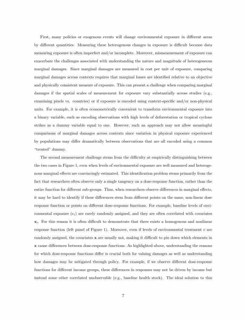
0 10 20 30 40 50 60 70Max cyclone wind speed experienced 1950−2008 (m/s)

Cum

ulat

ive

fract

ion

of p

opul

atio

n ex

pose

d to

cyc

lone

win

ds o

f les

ser o

r equ

al in

tens

ity

0

0.2

0.4

0.6

0.8

1

-10 0 10 20 30 40-5

0

5

10

Monthly mean temperature (°C)

Addi

tiona

l hum

an-m

onth

s pe

r yea

r (d

ensi

ty, 1

08 hu

man

-mon

ths

per °

C)

richest tercilemiddle tercilepoorest tercile

Global exposure to tropical cylonesin current climate, by income

Global exposure to changes in temperaturedue to climate change, by income

Tropical cyclones & GDP globallyby income

Years since storm

0 5 10 15 20

above median income

below median income

% G

DP c

umul

ative

loss

per

m/s

of c

yclo

ne e

xpos

ure

-0.3

-0.2

-0.1

0

0.1

-0.4

A B

C D

tropi

cal s

torm

cate

gory

1

cate

gory

2

cate

gory

3

0 500 1000 1500 2000 2500 3000-20

-10

0

10

20

30

40

Dire

ct d

amag

e pe

r cou

nty

(% o

f cou

nty

inco

me)

Counties by rank order of current income (poorest to richest per capita)

Climate change damage in USAby income

cate

gory

5

cate

gory

4

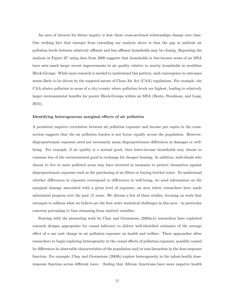
Figure 4: (A) Cumulative distribution function for maximum cyclone winds experienced under thecurrent climate for populations in terciles of the global income distribution (2000 est.): dotted=richest,dashed=middle, solid=poorest. Vertical lines indicate threshold maximum wind speeds on the Saffir-Simpson cyclone intensity scale (maximum value in sample is 78 m/s). Based on authors’ calculationsusing data from CIESIN (2005); Sala-i Martin (2006); Hsiang and Narita (2012). (B) Change in theexpected distribution of monthly temperatures experienced by the global population due to businessas usual warming by 2100. Based on authors’ calculation using data from Meehl et al. (2007); incometerciles are the same as in (A). Negative values indicate fewer months at a corresponding temperature,positive values indicate more moths at a corresponding temperature. (C) Homogeneous marginaldamages on GDP per capita growth (1970-2008) from one additional m/s of national average cycloneexposure for rich and poor countries; from Hsiang and Jina (2014). (D) Probabilistic projectionsof direct economic damage from business-as-usual warming (RCP8.5) by 2080-2099 for US countiesranked by their current incomes; from Hsiang et al. (2017). Circles are median estimates, dark whiskersare inner 67% of probability mass for each county, light whiskers are inner 90% of probability mass.

21

and drier locations, both within and across countries (Nordhaus, 2006; Park et al., 2015), there are

notable exceptions within countries (e.g., Florida, California, and Arizona in the United States), and

across countries (e.g., Singapore and major oil-producing countries in the Middle East). Furthermore,

some evidence suggests this cross-sectional association has changed over time (Acemoglu, Johnson,

and Robinson, 2002). Tropical countries, which tend to be poor, are the most exposed to the El Nino

Southern Oscillation (ENSO) (Hsiang and Meng, 2015), although wealthy Australia is notoriously

heavily exposed as well (Nicholls, 1989). Tropical cyclones (the class of phenomena including hurri-

canes, typhoons and tropical storms) tend to move away from the equator for physical reasons and

their baseline distribution across space is spread fairly evenly across global income categories—we show

this in the cumulative distribution function in Figure 4A, which we compute by overlaying the global

cyclone climatology from Hsiang and Narita (2012) on the global pixel-level population distribution

(CIESIN, 2005) sorted by their estimated location in the global income distribution from Sala-i Martin

(2006). Roughly 35% of the two poorer terciles are never exposed to a tropical cyclones, whereas 45%

of the richest tercile is never exposed. However, this high-income advantage reverses when the intensity

of cyclones is considered: a relatively larger fraction of the rich tercile is exposed to tropical cyclone

winds of any intensity above those equal to “tropical storm” status (according to the Saffir-Simpson

intensity scale). Current tornado climatologies represent perhaps the most extreme counter-example of

standard intuition: because the strong temperature and pressure gradients required to generate torna-

does only exist over land in the middle latitudes, tornado exposure is almost exclusive to populations

that are relatively wealthy (US, Europe, and Australia) or middle income (South Africa, Argentina,

and China) (Goliger and Milford, 1998).

The projected distribution of exposure to future climate changes with little or no mitigation is

also more complex than the simple notion that poor countries will face the largest quantities of ad-

verse exposure. There is negative correlation between current average income and the magnitude of

future average temperature changes across locations, and little correlation between income and rain-

fall changes. Average temperature changes (∆ei in the sense of Figure 1) are expected to be most

extreme in northern locations, which tend to be wealthier today, and lowest in the tropics (Stocker,

2014; Hsiang and Sobel, 2016). However, changes in exposure to extremely hot temperatures (e.g.,

> 30◦C), which are often thought to be the most damaging events, will be largest for the poorest

populations around the world. This is shown in Figure 4B, which shows the difference between the

probability distribution of temperature exposure in 2080-2099 under warming relative to the present.

22

These differences show how the expected experience of an individual drawn at random, from the global

income terciles computed above, change with warming. The largest positive change occurs for poor

and middle income terciles above > 29◦C, indicating that these individuals will experience many more

days at these very high temperatures.

Changes in future rainfall are substantially less certain and more mixed with no clear association

with current income (Stocker, 2014), since the deep tropics and high latitudes get wetter while sub-

tropics tend to dry out. Changes in future tropical cyclone distributions are similarly unrelated to

current incomes, with the strongest intensification expected in the East Asia, weakening in the Indian

ocean, and unclear changes in the Atlantic (Knutson et al., 2010). Thus, overall, there is little support

for the notion that exposure to future climate changes are inherently greater for poorer populations.

However, once one accounts for the potentially heterogeneous marginal effects of these changes, future

damages seem likely to be larger for poor populations.

Identifying heterogeneous marginal effects of climate

Dose-responses from climatic conditions are usually compared among contemporaries across different

locations, such as vulnerability across different counties (e.g., Annan and Schlenker (2015)) or countries

(e.g., Hsiang, Meng, and Cane (2011)), or within a fixed location but varying over time (e.g., Roberts

and Schlenker (2011)). When examining contemporaries, the core question is usually either (i) whether

some social or economic attribute of a population, such as higher income and stronger institutions (e.g.,

Dell, Jones, and Olken (2012)), cause them to suffer larger or smaller responses from climatic exposure,

or (ii) whether populations more regularly exposed to a specific type of climate are better equipped

to cope with the type of events characteristic of that climate (e.g., Hsiang and Narita (2012)). In

this second case, the intuition is that if populations experience a climatic event more frequently, they

may have learned about that event and invested in precautions that will limit their losses each time

the event occurs. A similar intuition holds when examining how marginal effects evolve with time,

since populations may gradually learn about their climate and then develop and deploy technologies

to cope with specific events they expect to occur, causing their marginal losses to gradually decrease.

All of these comparisons are primarily descriptive and cannot usually be interpreted as causal, since

there is not exogenous variation in those factors that might be determinants of vulnerability. However,

Hsiang, Burke, and Miguel (2013) point out that in some contexts a potential cause of vulnerability

could be credibly identified (or ruled out) if some exogenous change causes a key channel to appear for

23

the first time or to be abruptly obstructed if it was already present, and a corresponding sharp change

(or absence of change) in marginal losses is observed at that moment. Some recent examples of this

approach include the demonstration that work-for-pay programs in India reduce the sensitivity of local

violence to rainfall (Fetzer, 2014) and the sensitivity of child test scores to temperature (Garg, Jagani,

and Taraz, 2017). Also, Sarsons (2015) shows that access to dams does not alter the rainfall-violence

link in India. Hornbeck and Keskin (2014) found that new irrigation technologies reduced US farmers’

sensitivity to drought when they also had access to a major aquifer, and Barreca et al. (2016) provide

evidence that the introduction and deployment of air-conditioning technologies reduced the marginal

impact of temperature on mortality in the US.

In many cases where dose-responses are observed to differ significantly across populations, economic

explanations may be consistent with these patterns. For example, Hsiang and Narita (2012) show how

high spatial concentration of capital in rich countries may lead to higher defensive investment and

lower responsiveness from cyclones, and Davis and Gertler (2015) demonstrate patterns of climate-

related energy demand may reflect the influence of income on air-conditioning demand. Some patterns

of heterogeneity suggest the existence of additional market failures. Credit constraints likely bind in

many lower income contexts, causing individuals to under-invest in protective measures (Burgess et al.,

2011) or adopt ex-post coping strategies that may be effective in the short run but extremely costly

in the long run, such as disinvesting in children (Maccini and Yang, 2009; Anttila-Hughes and Hsiang,

2011) or engaging in transactional sex (Burke, Gong, and Jones, 2015).

In numerous cases, as documented by Carleton and Hsiang (2016), dose-response functions are

similar between low and high income countries. For example, a frequent observation is that rich and

poor populations respond to certain types of climate exposure with similar marginal losses, when one

might expect wealthy populations to be more adapted and thus exhibit lower climate sensitivity. For

example, Figure 4C displays the long-run effect of tropical cyclones on GDP growth from Hsiang and

Jina (2014), where relative income losses per unit of exposure for rich and poor countries appear to

be almost identical. Understanding why such adaptation gaps persist in some cases and not others is

an important challenge for future research.

Other than looking at the role of income, another line of inquiry is to ask whether learning shapes

marginal effects by comparing dose-response functions from short-lived vs. gradual changes (Dell,

Jones, and Olken, 2012; Burke, Emerick et al., 2016). This class of analysis attempts to determine

whether observed differences in responsivness within a population are due to experience and subsequent

24

adaptation; the hope is that such insight might also explain differences in climate sensitivity across

populations. The motivation for this comparison is the intuition that if populations can endogenously

alter their sensitivity through learning and adaptation in the long run, the marginal effects of slow

climate changes should be less damaging than those of unexpected short-lived events (Shrader, 2016).

However, if the observed marginal effects are similar across these cases, that may suggest limited

scope for effective adaptations (Moore and Lobell, 2014). A continuous version of this approach is

to filter time series or panel data at all temporal frequencies and estimate climate sensitivity at each

frequency of climatic variation (Hsiang, 2016). Despite these efforts, the literature has had limited

success pinning down systematic patterns for the relationship between climate sensitivity at short and

long time scales.

Separate from any notion of adaptation, another major source of heterogeneity in climate sensitivity

stem from nonlinearities in the dose-response function—a relationship that may be more mechanical in

nature than indicative of deeper economic dynamics. Nonlinear responses to climate have been care-

fully identified in a number of contexts, whether examining effects of climate on crop yields (Schlenker

and Roberts, 2009b; Schlenker and Lobell, 2010), mortality (Deschenes and Greenstone, 2011), energy

demand (Aroonruengsawat and Auffhammer, 2011), social instability (Hidalgo et al., 2010), prop-

erty crime (Ranson, 2014), permanent migration (Bohra-Mishra, Oppenheimer, and Hsiang, 2014),

labor supply (Graff Zivin and Neidell, 2014), human emotion (Baylis, 2015), cognitive performance

(Graff Zivin, Hsiang, and Neidell, forthcoming), human capital formation (Park, 2017), or income

(Deryugina and Hsiang, 2014; Isen, Rossin-Slater, and Walker, 2017). In these cases, the baseline

climate of a population may play a large role in determining the marginal damages from climate

simply because the population’s initial position on the dose-response function may exhibit a steeper

or shallower slope. Burke, Hsiang, and Miguel (2015) demonstrate the importance of this issue by

showing that a nonlinear relationship between temperature and economic growth appears statistically

similar to a situation where poor countries have large negative marginal effects of temperature be-

cause they are poor (i.e. because poor countries are also systematically hotter than rich countries).

However, the economic projections (or counterfactuals) under global warming differ dramatically de-

pending on whether heterogeneity is assumed to be caused by income or by non-linear temperature

responses. Frequently, the strong correlation between the economic characteristics of populations and

their baseline climates makes it exceptionally challenging to determine which drives heterogeneity

in marginal damages. Furthermore, it is also possible that these nonlinear dose-response functions

25

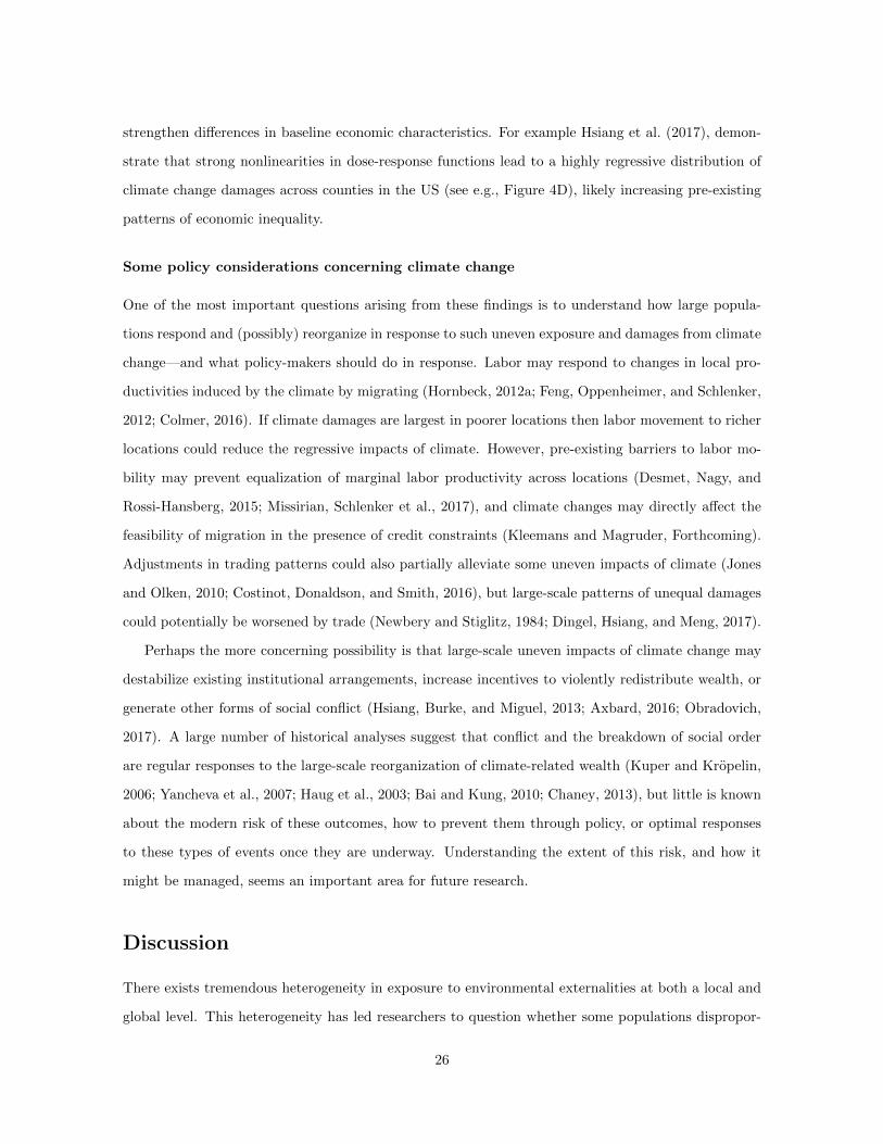
strengthen differences in baseline economic characteristics. For example Hsiang et al. (2017), demon-

strate that strong nonlinearities in dose-response functions lead to a highly regressive distribution of

climate change damages across counties in the US (see e.g., Figure 4D), likely increasing pre-existing

patterns of economic inequality.

Some policy considerations concerning climate change

One of the most important questions arising from these findings is to understand how large popula-

tions respond and (possibly) reorganize in response to such uneven exposure and damages from climate

change—and what policy-makers should do in response. Labor may respond to changes in local pro-

ductivities induced by the climate by migrating (Hornbeck, 2012a; Feng, Oppenheimer, and Schlenker,

2012; Colmer, 2016). If climate damages are largest in poorer locations then labor movement to richer

locations could reduce the regressive impacts of climate. However, pre-existing barriers to labor mo-

bility may prevent equalization of marginal labor productivity across locations (Desmet, Nagy, and

Rossi-Hansberg, 2015; Missirian, Schlenker et al., 2017), and climate changes may directly affect the

feasibility of migration in the presence of credit constraints (Kleemans and Magruder, Forthcoming).

Adjustments in trading patterns could also partially alleviate some uneven impacts of climate (Jones

and Olken, 2010; Costinot, Donaldson, and Smith, 2016), but large-scale patterns of unequal damages

could potentially be worsened by trade (Newbery and Stiglitz, 1984; Dingel, Hsiang, and Meng, 2017).

Perhaps the more concerning possibility is that large-scale uneven impacts of climate change may

destabilize existing institutional arrangements, increase incentives to violently redistribute wealth, or

generate other forms of social conflict (Hsiang, Burke, and Miguel, 2013; Axbard, 2016; Obradovich,

2017). A large number of historical analyses suggest that conflict and the breakdown of social order

are regular responses to the large-scale reorganization of climate-related wealth (Kuper and Kropelin,

2006; Yancheva et al., 2007; Haug et al., 2003; Bai and Kung, 2010; Chaney, 2013), but little is known

about the modern risk of these outcomes, how to prevent them through policy, or optimal responses

to these types of events once they are underway. Understanding the extent of this risk, and how it

might be managed, seems an important area for future research.

Discussion

There exists tremendous heterogeneity in exposure to environmental externalities at both a local and

global level. This heterogeneity has led researchers to question whether some populations dispropor-

26

tionately bear the burden of environmental damages, with substantial concern that poor populations

are differentially harmed. Recent econometric work has clarified some cases in which this is true and

others in which the data run counter to this intuition. A pervasive difficulty in the interpretation

of previous literature that documents heterogeneity in dose-response functions by income is that, in

many cases, it remains unclear whether the heterogeneity stems from differences in exposure levels

or differences in the structure of the response function across populations. The possible presence

of nonlinear response functions and non-uniform exposure complicates the determination of whether

marginal damages fundamentally differ across groups, especially when exogenous variation in factors

that might affect responsiveness is absent. Understanding the underlying source of heterogeneity in

dose-response functions is important to understand the benefits of future policy decisions. We see the

investigation into the underlying causal determinants of heterogeneity in dose-response functions as

being a key research area going forward.

A second difficulty that often arises in this literature is translating damages measured in physical

quantities, such as “number of deaths” or “acres of forest cleared,” into welfare measures that may be

compared across contexts and outcomes. This is especially true when there are unobserved tradeoffs

made by individuals in a market equilibrium, which may implicitly compensate individuals for their

willingness to tolerate increased exposures and/or risk (Rosen, 1974). In some cases, researchers have

turned to hedonic approaches that deliver results which can be interpreted in welfare terms under some

assumptions. In other cases, researchers assign standardized valuations to physical quantities, such

as valuing statistical lives, although such valuations may not always be well identified or grounded

in empirical observations. Despite these efforts, it is widely understood that these solutions are in-

complete and/or not universally applicable. Thus, developing robust and generalizable approaches for

recovering empirical welfare measures of non-market amenities is currently a core frontier problem in

understanding the distribution of environmental damages.

We close by posing a challenge to researchers. The finding that poor populations, in many contexts,

might be differentially exposed or impacted by environmental conditions suggests one of the most dif-

ficult but (potentially) important unanswered questions in this research space: Do any environmental

damages have impacts long-lasting enough to generate persistent feedback loops? For example, if being

poorer causes households to suffer relatively larger losses from the environment, then can this damage

in turn cause that household to be poorer and suffer larger losses yet again in the next generation?

Such feedbacks would be important to identify, since they may give rise to long-run compounding

27

distributional consequences with potentially large welfare implications. Compelling empirical evidence

of any such a feedback loop is lacking, but there exist some cases where cross-sectional—and possibly

long-run—patterns are similar in sign or structure to the short-run effects that the empirical liter-

ature has mostly focused on. For example, nonlinear cross-sectional distributions of income across

temperatures (Nordhaus, 2006) are broadly consistent with short-run effects of temperature on income

growth (Burke, Hsiang, and Miguel, 2015). Similarly, some of the most impoverished regions of the

United States are areas with the highest levels of ambient air pollution (Spira-Cohen et al., 2010,

2011). However, in both cases, it remains completely unknown if any of these observed cross-sectional

relationships match the short-run evidence coincidentally or causally. Could environmental factors

be a key driver for the distribution of wealth we observe in the world today? Credibly identifying

such long-run effects will likely require that we deeply understand the long-run dynamic response to

environmental conditions, a problem that we believe is the most valuable target for future inquiry.

ReferencesAcemoglu, D., S. Johnson, and J. A. Robinson. 2001. “The Colonial Origins of Comparative Develop-

ment: An Empirical Investigation.” American Economic Review 91 (5):1369–1401.

Acemoglu, Daron, Simon Johnson, and James A Robinson. 2002. “Reversal of fortune: Geographyand institutions in the making of the modern world income distribution.” The Quarterly Journal ofEconomics 117 (4):1231–1294.

Adger, W Neil. 2006. “Vulnerability.” Global environmental change 16 (3):268–281.

Albouy, David, Walter Graf, Ryan Kellogg, and Hendrik Wolff. 2016. “Climate Amenities, ClimateChange, and American Quality of Life.” Journal of the Association of Environmental and ResourceEconomists 3 (1):205–246.

Alix-Garcia, Jennifer M, Katharine RE Sims, and Patricia Yanez-Pagans. 2015. “Only one tree fromeach seed? Environmental effectiveness and poverty alleviation in Mexico’s Payments for EcosystemServices Program.” American Economic Journal: Economic Policy 7 (4):1–40.

Andam, Kwaw S, Paul J Ferraro, Katharine RE Sims, Andrew Healy, and Margaret B Holland. 2010.“Protected areas reduced poverty in Costa Rica and Thailand.” Proceedings of the National Academyof Sciences 107 (22):9996–10001.

Angrist, Joshua D and Jorn-Steffen Pischke. 2010. “The credibility revolution in empirical economics:How better research design is taking the con out of econometrics.” The Journal of economic per-spectives 24 (2):3–30.

Annan, Francis and Wolfram Schlenker. 2015. “Federal crop insurance and the disincentive to adaptto extreme heat.” The American Economic Review 105 (5):262–266.

Anthoff, David, Cameron Hepburn, and Richard SJ Tol. 2009. “Equity weighting and the marginaldamage costs of climate change.” Ecological Economics 68 (3):836–849.

Anttila-Hughes, Jesse K. and Solomon M. Hsiang. 2011. “Destruction, Disinvestment, and Death:Economic and Human Losses Following Environmental Disaster.” Working paper .

Arceo, Eva, Rema Hanna, and Paulina Oliva. 2016. “Does the Effect of Pollution on Infant MortalityDiffer Between Developing and Developed Countries? Evidence from Mexico City.” The EconomicJournal 126 (591):257–280.

28

Aroonruengsawat, Anin and Maximilian Auffhammer. 2011. “Impacts of climate change on residen-tial electricity consumption: evidence from billing data.” In The Economics of climate change:Adaptations past and present. University of Chicago Press, 311–342.

Auffhammer, Maximilian, Solomon Hsiang, Wolfram Schlenker, and Adam Sobel. 2013. “Using weatherdata and climate model output in economic analyses of climate change.” Review of EnvironmentalEconomics and Policy 7 (2):181–198.

Axbard, Sebastian. 2016. “Income Opportunities and Sea Piracy in Indonesia: Evidence from SatelliteData.” American Economic Journal: Applied Economics 8 (2):154–94.

Bai, Y and J.K Kung. 2010. “Climate Shocks and Sino-nomadic Conflict.” The Review of Economicsand Statistics 93 (3):970–981.

Banzhaf, Spencer H and Randall P Walsh. 2008. “Do people vote with their feet? An empirical testof Tiebout’s mechanism.” The American Economic Review 98 (3):843–863.

Barreca, Alan, Karen Clay, Olivier Deschenes, Michael Greenstone, and Joseph S Shapiro. 2016.“Adapting to climate change: The remarkable decline in the US temperature-mortality relationshipover the twentieth century.” Journal of Political Economy 124 (1):105–159.

Bartik, Timothy J. 1988. “Evaluating the benefits of non-marginal reductions in pollution usinginformation on defensive expenditures.” Journal of Environmental Economics and Management15 (1):111–127.

Baumol, William J and Wallace E Oates. 1988. The theory of environmental policy. Cambridgeuniversity press.

Baylis, Patrick. 2015. “Temperature and temperament: Evidence from a billion tweets.” EnergyInstitute at HAAS working paper .

Been, Vicki and Francis Gupta. 1997. “Coming to the nuisance or going to the barrios-a longitudinalanalysis of environmental justice claims.” Ecology LQ 24:1.

Bento, Antonio, Matthew Freedman, and Corey Lang. 2015. “Who benefits from environmental regula-tion? evidence from the clean air act amendments.” Review of Economics and Statistics 97 (3):610–622.

Bento, Antonio M. 2013. “Equity impacts of environmental policy.” Annual Review of ResourceEconomics 5 (1):181–196.

Bianchi, FJJA, PW Goedhart, and JM Baveco. 2008. “Enhanced pest control in cabbage crops nearforest in The Netherlands.” Landscape Ecology 23 (5):595–602.

Bohra-Mishra, Pratikshya, Michael Oppenheimer, and Solomon M. Hsiang. 2014. “Nonlinear perma-nent migration responses to climatic variations but minimal response to disasters.” Proceedings ofthe National Academy of Sciences 111 (27):9780–9785.

Brooks, Nancy and Rajiv Sethi. 1997. “The distribution of pollution: community characteristics andexposure to air toxics.” Journal of Environmental Economics and Management 32 (2):233–250.

Burgess, Robin, Olivier Deschenes, Dave Donaldson, and Michael Greenstone. 2011. “Weather anddeath in India.” Working paper .

Burke, Marshall, Kyle Emerick et al. 2016. “Adaptation to Climate Change: Evidence from USAgriculture.” American Economic Journal: Economic Policy 8 (3):106–40.

Burke, Marshall, Erick Gong, and Kelly Jones. 2015. “Income shocks and HIV in Africa.” TheEconomic Journal 125 (585):1157–1189.

Burke, Marshall, Solomon M Hsiang, and Edward Miguel. 2015. “Global non-linear effect of temper-ature on economic production.” Nature 527 (7577):235–239.

Carleton, Tamma A and Solomon M Hsiang. 2016. “Social and economic impacts of climate.” Science353 (6304):aad9837.

29

Chaney, Eric. 2013. “Revolt on the Nile: Economic shocks, religion, and political power.” Econometrica81 (5):2033–2053.

Chay, Kenneth Y and Michael Greenstone. 2003a. “Air quality, infant mortality, and the Clean AirAct of 1970.” Tech. rep., National Bureau of Economic Research.

———. 2003b. “The Impact of Air Pollution on Infant Mortality: Evidence from Geographic Variationin Pollution Shocks Induced by a Recession.” The Quarterly Journal of Economics :1121–1167.

CIESIN. 2005. “Gridded Population of the World, Version 3 (GPWv3): Subnational AdministrativeBoundaries.” URL http://dx.doi.org/10.7927/H4P26W1B.

Clark, Lara P, Dylan B Millet, and Julian D Marshall. 2014. “National patterns in environmentalinjustice and inequality: outdoor NO2 air pollution in the United States.” PloS one 9 (4):e94431.

Colmer, Jonathan. 2016. “Weather, labour reallocation, and industrial production: Evidence fromindia.” Work. Pap., London Sch. Econ., London .

Conte, Marc N and Matthew J Kotchen. 2010. “Explaining the price of voluntary carbon offsets.”Climate Change Economics 1 (02):93–111.

Costinot, Arnaud, Dave Donaldson, and Cory Smith. 2016. “Evolving comparative advantage andthe impact of climate change in agricultural markets: Evidence from 1.7 million fields around theworld.” Journal of Political Economy 124 (1):205–248.

Courant, Paul N and Richard C Porter. 1981. “Averting expenditure and the cost of pollution.”Journal of Environmental Economics and Management 8 (4):321–329.

Cropper, Maureen and Charles Griffiths. 1994. “The interaction of population growth and environ-mental quality.” The American Economic Review 84 (2):250–254.

Currie, Janet. 2011. “Inequality at Birth: Some Causes and Consequences.” The American EconomicReview 101 (3):1–22.

Currie, Janet and Matthew Neidell. 2005. “Air pollution and infant health: what can we learn fromCalifornia’s recent experience?” The Quarterly Journal of Economics 120 (3):1003–1030.

Currie, Janet and Reed Walker. 2011. “Traffic congestion and infant health: Evidence from E-ZPass.”American Economic Journal: Applied Economics 3 (1):65–90.

Davis, Lucas W. 2011. “The effect of power plants on local housing values and rents.” Review ofEconomics and Statistics 93 (4):1391–1402.

Davis, Lucas W and Paul J Gertler. 2015. “Contribution of air conditioning adoption to future energyuse under global warming.” Proceedings of the National Academy of Sciences 112 (19):5962–5967.

Dell, Melissa, Benjamin F. Jones, and Benjamin A. Olken. 2012. “Temperature Shocks and EconomicGrowth: Evidence from the Last Half Century.” American Economic Journal: Macroeconomics4 (3):66–95.

Depro, Brooks, Christopher Timmins, and Maggie O’Neil. 2015. “White flight and coming to thenuisance: can residential mobility explain environmental injustice?” Journal of the Association ofEnvironmental and resource Economists 2 (3):439–468.

Deryugina, Tatyana and Solomon M Hsiang. 2014. “Does the environment still matter? Daily tem-perature and income in the United States.” Tech. rep., National Bureau of Economic Research.

Deryugina, Tatyana, Laura Kawano, and Steven Levitt. Forthcoming. “The economic impact of hur-ricane katrina on its victims: evidence from individual tax returns.” American Economic Journal:Applied Economics .

Deschenes, Olivier and Michael Greenstone. 2007. “The economic impacts of climate change: evidencefrom agricultural output and random fluctuations in weather.” The American Economic Review97 (1):354–385.

30

———. 2011. “Climate Change, Mortality, and Adaptation: Evidence from Annual Fluctuations inWeather in the US.” American Economic Journal: Applied Economics 3 (4):152–85.

Deschenes, Olivier, Michael Greenstone, and Joseph S Shapiro. Forthcoming. “Defensive investmentsand the demand for air quality: Evidence from the nox budget program and ozone reductions.”American Economic Review .

Deschenes, Olivier and Enrico Moretti. 2009. “Extreme weather events, mortality and migration.” TheReview of Economics and Statistics 91:659–681.

Desmet, Klaus, David Krisztian Nagy, and Esteban Rossi-Hansberg. 2015. “The geography of devel-opment: Evaluating migration restrictions and coastal flooding.” Tech. rep., National Bureau ofEconomic Research.

Diamond, Peter A and Jerry A Hausman. 1994. “Contingent valuation: Is some number better thanno number?” The Journal of economic perspectives 8 (4):45–64.

Dingel, Jonthan, Solomon Hsiang, and Kyle Meng. 2017. “The Spatial Structure of Endowments,Trade, and Inequality: Evidence from the Global Climate.” working paper .

Ebert, Udo. 2003. “Environmental goods and the distribution of income.” Environmental and ResourceEconomics 25 (4):435–459.

Feng, S., M. Oppenheimer, and W. Schlenker. 2012. “Climate Change, Crop Yields, and InternalMigration in the United States.” Tech. rep., National Bureau of Economic Research.

Fetzer, Thiemo. 2014. “Social insurance and conflict: evidence from India.” .

Flores, Nicholas E and Richard T Carson. 1997. “The relationship between the income elasticities ofdemand and willingness to pay.” Journal of Environmental Economics and Management 33 (3):287–295.

Fowlie, Meredith, Stephen P Holland, and Erin T Mansur. 2012. “What do emissions markets deliverand to whom? Evidence from Southern California’s NOx trading program.” The American economicreview 102 (2):965–993.

Frank, Eyal G and Wolfram Schlenker. 2016. “Balancing economic and ecological goals.” Science353 (6300):651–652.

Freeman, A Myrick. 1974. “On estimating air pollution control benefits from land value studies.”Journal of Environmental Economics and Management 1 (1):74–83.

Fullerton, Don. 2011. “Six distributional effects of environmental policy.” Risk analysis 31 (6):923–929.

———. 2017. Distributional effects of environmental and energy policy. Routledge.

Gallup, John Luke, Jeffrey D Sachs, and Andrew D Mellinger. 1999. “Geography and economicdevelopment.” International regional science review 22 (2):179–232.

Garg, Teevrat. 2014. “Public Health Effects of Natural Resource Degradation: Evidence from Indone-sia.” Working paper .

Garg, Teevrat, Maulik Jagani, and Vis Taraz. 2017. “Human Capital Costs of Climate Change:Evidence from Test Scores in India.” Mimeo .

Goliger, AM and RV Milford. 1998. “A review of worldwide occurrence of tornadoes.” Journal ofWind Engineering and Industrial Aerodynamics 74:111–121.

Graff Zivin, Joshua, Solomon Hsiang, and Matthew Neidell. forthcoming. “Temperature and HumanCapital in the Short- and Long-Run.” Journal of the Association of Environmental and ResourceEconomists .

Graff Zivin, Joshua and Matthew Neidell. 2014. “Temperature and the allocation of time: Implicationsfor climate change.” Journal of Labor Economics 32 (1):1–26.

Grainger, Corbett A. 2012. “The distributional effects of pollution regulations: Do renters fully payfor cleaner air?” Journal of Public Economics 96 (9):840–852.

31

Greenstone, Michael and B Kelsey Jack. 2015. “Envirodevonomics: A research agenda for an emergingfield.” Journal of Economic Literature 53 (1):5–42.

Grieg-Gran, Maryanne, Ina Porras, and Sven Wunder. 2005. “How can market mechanisms for forestenvironmental services help the poor? Preliminary lessons from Latin America.” World development33 (9):1511–1527.

Grossman, Michael. 1972. “On the Concept of Health Capital and the Demand for Health.” Journalof Political Economy 80(2):223–255.

Hallegatte, Stephane, Marianne Fay, Mook Bangalore, Tamaro Kane, and Laura Bonzanigo. 2015.Shock waves: managing the impacts of climate change on poverty. World Bank Publications.

Hamilton, James T. 1993. “Politics and social costs: estimating the impact of collective action onhazardous waste facilities.” The RAND Journal of Economics :101–125.

Hanemann, W Michael. 1991. “Willingness to pay and willingness to accept: how much can theydiffer?” The American Economic Review 81 (3):635–647.

Hansen, Matthew C, Peter V Potapov, Rebecca Moore, Matt Hancher, SA Turubanova, AlexandraTyukavina, David Thau, SV Stehman, SJ Goetz, TR Loveland et al. 2013. “High-resolution globalmaps of 21st-century forest cover change.” Science 342 (6160):850–853.

Harrison, David and Daniel L Rubinfeld. 1978. “Hedonic housing prices and the demand for cleanair.” Journal of environmental economics and management 5 (1):81–102.

Haug, G.H, D Gunther, L.C Peterson, D.M Sigman, K.A Hughen, and B Aeschlimann. 2003. “Climateand the collapse of Maya civilization.” Science 299 (5613):1731.

Hidalgo, F.D, S Naidu, S Nichter, and N Richardson. 2010. “Economic determinants of land invasions.”The Review of Economics and Statistics 92 (3):505–523.

Hokby, Stina and Tore Soderqvist. 2003. “Elasticities of demand and willingness to pay for environ-mental services in Sweden.” Environmental and resource economics 26 (3):361–383.

Hornbeck, Richard. 2012a. “The Enduring Impact of the American Dust Bowl: Short-and Long-RunAdjustments to Environmental Catastrophe.” The American Economic Review 102 (4):1477–1507.

———. 2012b. “Nature versus Nurture: The Environment’s Persistent Influence through the Modern-ization of American Agriculture.” The American Economic Review 102 (3):245–249.

Hornbeck, Richard and Pinar Keskin. 2014. “The historically evolving impact of the ogallala aquifer:Agricultural adaptation to groundwater and drought.” American Economic Journal: Applied Eco-nomics 6 (1):190–219.

Hsiang, Solomon. 2016. “Climate econometrics.” Annual Review of Resource Economics 8:43–75.

Hsiang, Solomon, Robert Kopp, Amir Jina, , James Rising, Michael Delgado, DJ Rasmussen, ShashankMohan, Paul Wilson, Robert Muir-Wood, Michael Oppenheimer, Kate Larsen, and Trevor Houser.2017. “Estimating Economic Damage from Climate Change in the United States.” Science356 (6345):1362–1369.

Hsiang, Solomon M, Marshall Burke, and Edward Miguel. 2013. “Quantifying the influence of climateon human conflict.” Science 341 (6151):1235367.

Hsiang, Solomon M. and Amir S. Jina. 2014. “The Causal Effect of Environmental Catastrophe onLong-Run Economic Growth: Evidence From 6,700 Cyclones.” Working Paper 20352, NationalBureau of Economic Research.

Hsiang, Solomon M and Amir S Jina. 2015. “Geography, depreciation, and growth.” The AmericanEconomic Review 105 (5):252–256.

Hsiang, Solomon M and Kyle C Meng. 2015. “Tropical Economics.” American Economic Review105 (5):257–61.

32

Hsiang, Solomon M., Kyle C. Meng, and Mark A. Cane. 2011. “Civil conflicts are associated with theglobal climate.” Nature 476 (7361):438–441.

Hsiang, Solomon M. and Daiju Narita. 2012. “Adaptation to Cyclone Risk: Evidence from the GlobalCross-Section.” Climate Change Economics 3 (2).

Hsiang, Solomon M and Adam H Sobel. 2016. “Potentially Extreme Population Displacement andConcentration in the Tropics Under Non-Extreme Warming.” Scientific reports 6.

IPCC. 2014. Climate Change 2014–Impacts, Adaptation and Vulnerability: Regional Aspects. Cam-bridge University Press.

Isen, Adam, Maya Rossin-Slater, and Reed Walker. 2017. “The Relationship Between Season of Birth,Temperature Exposure, and Later Life Well-Being.” Working Paper .

Jayachandran, Seema. 2009. “Air quality and early-life mortality evidence from Indonesia’s wildfires.”Journal of Human resources 44 (4):916–954.

Jayachandran, Seema, Joost de Laat, Eric F. Lambin, and Charlotte Y. Stanton. 2016. “Cash forCarbon: Randomized Controlled Trial of Payments for Ecosystem Services to Reduce Deforestation.”NBER working paper series .

Jones, Benjamin and Benjamin Olken. 2010. “Climate shocks and exports.” American EconomicReview: Papers and Proceedings 100:454–459.

Kahn, Matthew E. 2005. “The Death Toll from Natural Disasters: the role of Income, Geography, andInstitutions.” The Review of Economics and Statistics 87:271–284.

Kahn, Matthew E and John G Matsusaka. 1997. “Demand for Environmental Goods: Evidence fromVoting Patterns on California Initiatives 1.” The Journal of Law and Economics 40 (1):137–174.

Karp, Daniel S, Chase D Mendenhall, Randi Figueroa Sandı, Nicolas Chaumont, Paul R Ehrlich,Elizabeth A Hadly, and Gretchen C Daily. 2013. “Forest bolsters bird abundance, pest control andcoffee yield.” Ecology letters 16 (11):1339–1347.

Kleemans, Marieke and Jeremy Magruder. Forthcoming. “Labour Market Responses To Immigration:Evidence From Internal Migration Driven By Weather Shocks.” Economic Journal .

Knutson, Thomas R, John L McBride, Johnny Chan, Kerry Emanuel, Greg Holland, Chris Landsea,Isaac Held, James P Kossin, AK Srivastava, and Masato Sugi. 2010. “Tropical cyclones and climatechange.” Nature Geoscience 3 (3):157–163.

Kristrom, Bengt and Pere Riera. 1996. “Is the income elasticity of environmental improvements lessthan one?” Environmental and resource Economics 7 (1):45–55.

Kuper, R and S Kropelin. 2006. “Climate-controlled Holocene occupation in the Sahara: motor ofAfrica’s evolution.” Science 313 (5788):803.

Larsen, Ashley E. 2013. “Agricultural landscape simplification does not consistently drive insecticideuse.” Proceedings of the National Academy of Sciences 110 (38):15330–15335.

Larsen, Ashley E, Steven D Gaines, and Olivier Deschenes. 2015. “Spatiotemporal variation in the rela-tionship between landscape simplification and insecticide use.” Ecological Applications 25 (7):1976–1983.

Li, Zhou and Gregory Veeck. 1999. “Forest resource use and rural poverty in China.” Forestryeconomics 4:80–102.

Maccini, Sharon and Dean Yang. 2009. “Under the weather: Health, schooling, and economic conse-quences of early-life rainfall.” The American Economic Review 99 (3):1006–1026.

Mauzerall, Denise L, Babar Sultan, Namsoug Kim, and David F Bradford. 2005. “NOx emissions fromlarge point sources: variability in ozone production, resulting health damages and economic costs.”Atmospheric Environment 39 (16):2851–2866.

McFadden, Daniel. 1994. “Contingent valuation and social choice.” American Journal of AgriculturalEconomics 76 (4):689–708.

33

Meehl, Gerald A., Curt Covey, Thomas Delworth, Mojib Latif, Bryant McAvaney, John F. B., Mitchell,Ronald J. Stouffer, and Karl E. Taylor. 2007. “The WCRP CMIP3 Multimodel Dataset: A NewEra in Climate Change Research.” Bulletin of the American Meterological Society 88:1383–1394.

Mehta, Aasha Kapur and Amita Shah. 2003. “Chronic poverty in India: Incidence, causes and policies.”World Development 31 (3):491–511.

Missirian, Anouch, Wolfram Schlenker et al. 2017. “Asylum Applications and Migration Flows.”American Economic Review 107 (5):436–440.

Moore, Frances C and David B Lobell. 2014. “Adaptation potential of European agriculture in responseto climate change.” Nature Climate Change 4 (7):610–614.

Muller, Nicholas Z and Robert Mendelsohn. 2009. “Efficient Pollution Regulation: Getting the PricesRight.” The American Economic Review :1714–1739.

Myers, Norman. 1997. “The world’s forests and their ecosystem services.” Nature’s Services: societaldependence on natural ecosystems :215–235.

Newbery, David MG and Joseph E Stiglitz. 1984. “Pareto inferior trade.” The Review of EconomicStudies 51 (1):1–12.

Nicholls, Neville. 1989. “Sea surface temperatures and Australian winter rainfall.” Journal of Climate2 (9):965–973.

Noack, Frederik, Sven Wunder, Arild Angelsen, and Jan Borner. 2016. “Responses to Weather andClimate.” World Bank Policy Research Working Paper .

Nordhaus, W. and J. Boyer. 2000. Warming the World: Economic Models of Global Warming. TheMIT Press.

Nordhaus, W. D. 2006. “Geography and macroeconomics: New Data and new findings.” Proceedingsof the National Academy of Sciences 103 (10).

Novotny, Eric V, Matthew J Bechle, Dylan B Millet, and Julian D Marshall. 2011. “Nationalsatellite-based land-use regression: NO2 in the United States.” Environmental science & technology45 (10):4407–4414.

Obradovich, Nick. 2017. “Climate change may speed democratic turnover.” Climatic Change140 (2):135–147.

Olmstead, Alan L. and Paul W. Rhode. 2011. “Adapting North American wheat production to climaticchallenges, 1839–2009.” Proceedings of the National Academy of Sciences 108 (2):480–485.

Park, Jisung. 2017. “Heat Stress and Human Capital Production.” Harvard University working paper.

Park, Jisung, Stephane Hallegatte, Mook Bangalore, and Evan Sandhoefner. 2015. “Households andheat stress: estimating the distributional consequences of climate change.” World Bank PolicyResearch Working Paper .

Parry, Ian WH, Hilary Sigman, Margaret Walls, and Roberton C Williams III. 2006. “The incidence ofpollution control policies.” The International Yearbook of Environmental and Resource Economics2006/2007 :1–42.

Ranson, Matthew. 2014. “Crime, weather and climate change.” J. Environ. Econ. Manage 67 (3):274–302.

Roberts, Michael J. and Wolfram Schlenker. 2011. The Evolution of Heat Tolerance of Corn: Impli-cations for Climate Change. University of Chicago Press, 225–251.

Rosen, Sherwin. 1974. “Hedonic prices and implicit markets: product differentiation in pure competi-tion.” Journal of political economy 82 (1):34–55.

Sala-i Martin, Xavier. 2006. “The World Distribution of Income: Falling Poverty and...Convergence,Period.” The Quarterly Journal of Economics 71:351–397.

34

Sarsons, Heather. 2015. “Rainfall and conflict: A cautionary tale.” Journal of development Economics115:62–72.

Schlenker, W and D Lobell. 2010. “Robust negative impacts of climate change on African agriculture.”Environmental Research Letters 5 (1).

Schlenker, Wolfram, W Michael Hanemann, and Anthony C Fisher. 2006. “The impact of globalwarming on US agriculture: an econometric analysis of optimal growing conditions.” Review ofEconomics and statistics 88 (1):113–125.

Schlenker, Wolfram and Michael Roberts. 2009a. “Nonlinear temperature effects indicate severe dam-ages to U.S. crop yields under climate change.” Proceedings of the National Academy of Sciences106 (37):15594–15598.

Schlenker, Wolfram and Michael J Roberts. 2009b. “Nonlinear temperature effects indicate severedamages to US crop yields under climate change.” Proceedings of the National Academy of Sciences106 (37):15594–15598.

Schlenker, Wolfram and W Reed Walker. 2015. “Airports, air pollution, and contemporaneous health.”The Review of Economic Studies :rdv043.

Shrader, Jeffrey. 2016. “Expectations and adaptation to environmental risks.” Tech. rep., Workingpaper.

Solow, Robert. 2012. “Sustainability: an economist’s perspective.” In Economics of the Environment,edited by Robert Stavins. W. W. Norton & Company.

Spira-Cohen, Ariel, Lung Chi Chen, Michaela Kendall, Ramona Lall, and George D Thurston. 2011.“Personal exposures to traffic-related air pollution and acute respiratory health among Bronxschoolchildren with asthma.” Environmental Health Perspectives 119 (4):559.

Spira-Cohen, Ariel, Lung Chi Chen, Michaela Kendall, Rebecca Sheesley, and George D Thurston.2010. “Personal exposures to traffic-related particle pollution among children with asthma in theSouth Bronx, NY.” Journal of Exposure Science and Environmental Epidemiology 20 (5):446–456.

Stocker, Thomas. 2014. Climate change 2013: the physical science basis: Working Group I contributionto the Fifth assessment report of the Intergovernmental Panel on Climate Change. CambridgeUniversity Press.

Sunderlin, William D and Thu Ba Huynh. 2005. Poverty alleviation and forests in Vietnam. CIFOR.

United Church of Christ. 1987. Toxic wastes and race in the United States: A national report on theracial and socio-economic characteristics of communities with hazardous waste sites. Commissionfor Racial Justice.

US GAO. 1983. “Siting of hazardous waste landfills and their correlation with racial and economicstatus of surrounding communities.” GAOfRCED-83-168. Washington, DC: US. General AccountingOffice .

Van, Phu Nguyen and Theophile Azomahou. 2007. “Nonlinearities and heterogeneity in environmentalquality: An empirical analysis of deforestation.” Journal of Development Economics 84 (1):291–309.

World Bank. 2017. Bringing resilience to scale : a work plan for the global facility for disaster reductionand recovery. World Bank Group.

Yancheva, Gergana, Norbert R Nowaczyk, Jens Mingram, Peter Dulski, Georg Schettler, J—[ouml]—rgF W Negendank, Jiaqi Liu, Daniel M Sigman, Larry C Peterson, and Gerald H Haug. 2007. “Influenceof the intertropical convergence zone on the East Asian monsoon.” Nature 445 (7123):74.

35