the dynamics of foreign portfolio investment and …

WORKING PAPER

THE DYNAMICS OF FOREIGN PORTFOLIO

INVESTMENT AND EXCHANGE RATE: AN

INTERCONNECTION APPROACH IN ASEAN

Ferry Syarifuddin

WP/ /2020

2020

This is a working paper, and hence it represents research in progress. This paper represents the opinions of the authors, and is the product of professional

research. It is not meant to represent the position or opinions of the Bank Indonesia. Any errors are the fault of the authors.

dimas_pw

Typewritten Text

8

1

The Dynamics of Foreign Portfolio Investment

and Exchange Rates: An Interconnection

Approach in ASEAN

Ferry Syarifuddin

Abstract

This paper examines the spatial dependence of foreign portfolio investment (FPI) inflows between ASEAN countries from 2002Q1-2018Q4

utilizing the spatial econometric approach. In particular, to enrich the results of our research we also review the relationship between exchange rates and

macroeconomic factors on the FPI in Indonesia. The empirical results show that there is a competitive relationship in FPI between ASEAN countries that indicates crowding out of FPI in the host country is most likely to occur when

third-country experiences crowding in its FPI inflow. We also show that the exchange rate dynamics in the host and third country do not significantly affect FPI in the host country. Furthermore, the results indicate that interest

rate differential, inflation, economic growth, and government debt rating in host countries, also inflation, economic growth, and government debt rating

in neighboring countries are responsible for the inflow of FPI into host countries in ASEAN. In the Indonesia case study, our empirical results show that exchange rates affect bond and equity inflows, and also exchange rate

volatility affects foreign equity markets and total portfolio inflows in Indonesia. In addition, we find the importance of interest rate differential and the VIX index for Indonesia's portfolios market.

Key words: Foreign portfolio investment, Exchange rates, Macroeconomics,

Spatial panel econometrics, Spillover effects

JEL Classification: F21, F31, F41, C21, R12

2

1. Background

Most of the countries in Southeast Asia (ASEAN) are developing countries which is

require the big funds, such as foreign portfolio investment, to boost their economy. The

expansion of foreign portfolios in ASEAN began after the 1990s when the stock market and

securities became essential in economic growth in the ASEAN region. The existence of a trade

agreement between ASEAN countries, through the signing of the ASEAN Free Trade Area

(AFTA) and the implementation of the ASEAN Investment Area (AIA) in 1998 and the

ASEAN Comprehensive Investment Agreement (ACIA) in 2012, has increased investment

flows to ASEAN and created a liberal, transparent, and competitive investment environment

in ASEAN. The removal of trade restrictions and international investment agreements has

increased investment by foreign investors. Therefore, the foreign portfolio in terms of liabilities

(FPI inflow) to ASEAN increased nearly sixteen times from US $ 3.2 billion in 2001 to US $

51 billion in 2017. In this regard, Indonesia was the largest FPI recipient country in ASEAN in

2017. However, the volatility of FPI in ASEAN began increasing after the 2008 global

economic crisis, indicating its vulnerability to a reversal.

Short-term capital inflows, such as foreign portfolio investment, often have a strong

relationship with exchange rate dynamics because their investments tend to be liquid and

flexible. There have been debates on the impact of changes in exchange rates towards foreign

portfolio investment flows. Studies by Garg & Dua (2014), Srinivasan & Kalaivani (2015),

Haider et al. (2016), Wong (2017), Anggitawati & Ekaputra (2020) suggested that an

appreciated exchange rate promotes portfolio investments because foreign investors receive an

additional return source and encourage them to invest by appreciating the exchange rate. The

opposite result was found by Bleaney & Greenaway (2001), which argues that the foreigners

will be motivated to invest in the host country when there is a devaluation in the host country

currency due to higher return. Studies by Baek (2006), Cenedese et al. (2014), and Singhania

& Saini (2018) had different perspective where they found no relationship the exchange rates

and portfolio investments by foreign investors. Moreover, Persson & Svensson (1989), Bleaney

& Greenaway (2001), and Garg & Dua (2014) found volatility in exchange rate has negative

and significant impact on inducing portfolio investment.

Another set of literature also focus on the host country interest rate differential along with

the exchange rate. According to the neoclassical theory, foreign capitals are attracted by interest

rate between countries. Capital flows from developed countries with abundant capital and low

returns to developing countries with capital scarcity and high returns (Ghosh et al., 2014).

Qureshi et al. (2012), Garg & Dua (2014), and Ghosh et al. (2014) has found that an increase

in the interest rate differential allows a surge in capital inflows. In addition, the literature that

analyzes the determinants of portfolio flows discussed the relative significance of domestic

factors along with the exchange rate and interest rate differential (e.g., Ahmed Hannan, 2018;

Ahmed & Zlate, 2014; Al-Smadi, 2018; Alwafi, 2017; Fratzscher, 2012; Kinda, 2010; Luitel

& Vanpée, 2018; Marouane, 2019; Verma & Prakash, 2011).

Economic integration creates interdependence between countries with abundant and lack

of capital, driving cross-border asset growth beyond the expansion of goods and services. With

higher technology advancement and faster information exchange, geographical distances have

become more artificial. Coval & Moskowitz (2016) reported that asymmetric information

makes geographic proximity beneficial to investors located near potential investments. They

benefit in terms of selecting stocks, meaning that geographic location, informed trade, and asset

prices are closely related.

To the best of our knowledge, we documented that the progress of the existing literature

was not adequately addressing the spatial inter-relation on FPI between regions within a

3

country with each other. First, conventional studies, such as traditional panel data model and

time-series model, are mostly used in existing study literatures, which in this regard holds the

geographical interdependence factors as exogenous when investigate the FPI's behaviors

empirically (Ahmed & Zlate, 2014; Garg & Dua, 2014; Haider et al., 2016; Rafi &

Ramachandran, 2018; Singhania & Saini, 2018; Srinivasan & Kalaivani, 2015). Traditional

panels and gravity models cannot capture the effects of third countries in examining the

portfolio flow determinants, hence a spatial panel data model is used to overcome this problem.

Due to the relationship or dependence on economic activities between countries, the effects of

spatial interaction between countries in a certain region unavoidable. Studies that discuss FPI

behavior influenced by third countries are still quite rare. Only two literature studies relate to

the spatial relationship of FPI by Chuang & Karamatov (2018) and Jory et al. (2018).

Second, many studies have examined the FPI inflow determinants in an economic union

(e.g. Baek (2006) for Asian and Latin American FPI inflow, Singhania & Saini (2018),

Fratzscher (2012) for developed and developing countries FPI inflow, Ghosh et al. (2014) and

Ahmed & Zlate (2014) for developing countries FPI inflow, and Waqas et al. (2015) for South

Asian countries FPI inflow). However, we have not found any research related to the

determinants of FPI in Southeast Asia (ASEAN) yet. Besides, the existence of the Master Plan

on ASEAN Connectivity (MPAC) 2025 which address the technical regulations for investment

in ASEAN Member States (explicitly covers portfolio investment) and also the creating of a

new regional dynamic that drives recent investment treaty policies for countries in the ASEAN

with other countries (e.g. Australia and New Zealand (2009), Korea (2009), China (2009), and

India (2014)) potentially to cause inter-related policy among ASEAN countries that possibly

generates the spatial relation in FPI.

Furthermore, this paper contributes to the current literature in two crucial ways. First,

this study can be scientifically beneficial by adding and enrich current literature on the

geographic investment phenomenon in the aspect of a broader set of spatial econometrics of

FPI inflows, especially for ASEAN case. Because of the cross-border investment tends to

create the investor’s decision to invest their portfolio in a specific location and establish

geographical interconnection between neighboring countries. Jory et al. (2018) argues that due

to the intertwined nature of demographic, location-specific, attachment-attributable factors

with financial and economic variables, it makes these factors endogenously determine portfolio

investment performance. Therefore, the discussions about the existence of spatial distribution

of third-country can no longer be ignored. Second, using the spatial spillover effect, this paper

adds complexity to the identification of the true nature of portfolio investment performances in

ASEAN. We provide new insights for policy practices and financial investors through the

evidence of the existence of geographical interdependence on international investment in

ASEAN region.

This research also reviews the relationship between exchange rates and macroeconomic

factors on FPI because Indonesia is one of the Southeast Asia countries with a fairly rapid

growth trend in portfolio investment, especially in the last ten years after the 2008 global

economic crisis. Based on Bloomberg, during the 1998 crisis, when Indonesia's spot exchange

rate depreciated from 2,879 in 1997 to 10,210 in 1998, portfolio investment inflows decreased

from USD 5.0 to USD -1.9 billion in 1996-1998. Before 1994, FPI's movement in Indonesia

was dominated by equity stocks and investment funds. After 1994, there was a reversal of the

foreign portfolio investment dominance from equity stocks and investment funds to debt

securities, boosting FPI's growth. After the 2000s, the equity stocks and investment funds

declined with negative growth of -2.5 billion USD and -3.7 billion USD in 2017 and 2018.

Therefore, it is vital to examine the factors that influence foreign portfolio inflows to Indonesia.

4

Based on the background stated above, there are two objectives of this research:

1. This research measures and analyzes the relationship between exchange rate dynamics

and several macroeconomic variables on foreign portfolio investment flows in ASEAN

countries by including the interconnection relationship between countries.

2. The study also measures and analyzes the exchange rate dynamics and several

macroeconomic factors that affect foreign portfolio investment in Indonesia.

5

2. Literature Studies

Many literature reviews discuss foreign capital inflow, a topic of interest to investors.

However, most research related to foreign capital inflows only focuses on foreign direct

investment flows. The factors that affect portfolio investment are rarely examined. Research

about the determinants of foreign portfolio investment, through the variable debt and equity

flows, is used by Chuang & Karamatov (2018), which examines the relationship between the

growth of a country's stock market and the amount of connectivity in a network using spatial

panels in 21 countries. Focusing on the determinants of foreign portfolio investment through

debt and equity flows, the results showed a correlation between the growth of a country's stock

market and its closest countries. There was also a positive relationship with the country's

international investment, shown by debt securities.

Various approaches are used to examine the determinants of foreign portfolio investment

(FPI). The portfolio is often divided into three categories, including country, industry, and firm

levels. Most research focuses specifically on the country-level, specifically the relationship

between exchange rates and foreign portfolio investment flows, including Garg & Dua (2014),

Anggitawati & Ekaputra (2018), dan Caporale et al. (2017), Gumus et al. (2013). Garg & Dua

(2014), using a sample of India and the ARDL method, established that portfolio inflows were

influenced by lower exchange rate volatility and appreciation, and greater risk diversification

opportunities. Furthermore, it also disaggregates FPI into two, Foreign Institutional Investment

flows (FII) and American / Global Depository Receipts (ADR / GDR). The FII determinants

are similar to aggregate portfolio flows, while ADR / GDR is influenced by returns on domestic

equity, exchange rates, and domestic and foreign output growth. This is in line with

Anggitawati & Ekaputra (2018)., which established a causal relationship between net foreign

investment and the exchange rate in Indonesia using the VAR method. The increase in FPI in

form of domestic bonds often strengthens the local exchange rate. Domestic appreciation tends

to increase FPI in the bond market. In the domestic stock market, there is only a one-way

relationship, where only the domestic exchange rate has a significant impact on FPI movements

on the Indonesian stock market. In this regard, the FPI on the stock market does not affect the

domestic exchange rate. These results contravene Gumus et al. (2013), which established that

FPI is only influenced by the industrial production index, rather than the exchange rate.

Furthermore, shocks to portfolio investment affect the Istanbul stock price index and the

exchange rate.

French & Vishwakarma (2013) and Rafi & Ramachandran (2018) examined the effect of

FPI volatility on exchange rates. Using a sample of the Philippines and the SVARX-GARCH

method, French & Vishwakarma (2013) established that a shock in foreign capital flows to the

Philippines increased volatility in the stock market significantly over the next two weeks of

trading time. Furthermore, the shock also increased the variance of the USD / PHP exchange

rate for the next two to three weeks of trading time. This is in line with Rafi & Ramachandran

(2018), which examined the relationship between capital flows and exchange rate volatility in

developing countries using the VAR panel method. The results show an impulse response to

the shock effect in portfolio capital flows on exchange rate volatility, which increases

significantly compared to direct foreign inflows. The variance in shocks towards foreign

portfolio investment flows has a significant impact on exchange rate volatility. The variations

in current account balances, stock prices, and interest rates also affect exchange rate volatility.

Caporale et al. (2017), using the GARCH method and the Markov regime-switching, also

established that high exchange rate volatility is associated with equity (bond) inflows from

Asian countries to the US in all cases, except the Philippines.

6

Apart from focusing on the exchange rate, several studies also examined other

macroeconomic factors influencing FPI flows into a country by dividing them into two push

and pull variables. Push factors are represented as determinants of global liquidity conditions

and other factors that can drive investment flows into the country. In comparison, domestic

pull factors can be represented as risk and return. According to Baek (2006), there were

differences in the factors that pushed FPI to enter Asia and Latin America. In Asia, the FPI

inflow is driven by investor interest in risk and other external factors, while the pull factor from

the domestic can be ignored. Pull and push factors, such as strong economic growth and foreign

financial variables are the determining factors for the entry of FPI in America. However, FPI

in Latin America is not driven by market risk appetite. The FPI flowing in Asia is "hot" money

because it is sensitive to changes in global market conditions and external factors.

Using the ARDL method, Srinivasan & Kalaivani (2015) examined the FII determinants

in India. The returns on the Indian equity market have a negative short-term and a positive

long-term effect on FII inflows. The returns on US equity markets have a positive and

significant effect on FII flows in the long term but a positive and insignificant effect in the

short term. Furthermore, the exchange rate and domestic inflation also determine the FII inflow

to India. Using a sample of developed and developing countries and comparing static panel

models and GMM, Singhania & Saini (2018) examined the FPI determinants. The result, using

a static panel in developed countries showed that FPI inflows are determined by interest rate

differentials, trade openness, and stock market performance of the host country, while the US

stock market return is the significant trend determinant. In developing countries, the index of

freedom, differences in interest rates, the stock market performance in the host country, trade

openness, returns on the US stock market, and the crisis period (2006-2008) significantly

affected FPI inflows. Using the GMM model in 19 countries, a study showed that differences

in interest rates, freedom index, US and host country’s stock market returns significantly affect

portfolio investment.

Ghosh et al. (2014) used the probit method, 2SLS and country fixed effect and established

that lower US interest rates, a greater appetite for global risk, and the attractiveness of the

country attract capital inflows to developing countries. This is in line with Ahmed & Zlate

(2014), which determined the factors influencing capital flows in developing countries using

the static panel data method. The study established that driving factors, such as differences in

interest rates in developing and developed countries, global risks, and US policies influence

capital inflows significantly. Fratzscher (2012) showed that driving factors, such as shocks to

liquidity, risk, microeconomic conditions and policies in developed countries, especially the

United States, significantly affected capital flows to developing and developed countries during

the crisis period. During the 2007-2008 financial crisis period, these factors had a greater

influence on foreign capital inflows. Furthermore, the importance of pull factors, such as good

economic policies in a country and increased institutional arrangements to reject the risk of

external shocks affecting the incoming FPI were discovered.

Using a sample of South Asian country data and the GARCH method, Waqas et al. (2015)

determined the FPI flows determinants through pull factors. The results showed that lower

volatility in international portfolio flows was associated with high-interest rates, currency

depreciation, foreign direct investment, lower inflation, and higher GDP growth rates than the

host country. According to Al-Smadi (2018), a good and stable macroeconomic environment

in Jordan attract investors. Furthermore, high-risk diversification opportunities, adequate

liquidity, and a well-organized environment attract more portfolio investment. According to

Haider et al. (2016), GDP and foreign debt are strong determinants of FPI flows to China.

Furthermore, the exchange rate and population significantly influence FPI. Bhasin &

Khandelwal (2019) established that domestic and global factors most influencing foreign

7

capital inflows in India include returns from the MSCI index, past FII values, and economic

growth rates.

Ouedraogo (2017) specifically examined the factors influencing FPI focusing on the

industry-level. The study determined the relationship between portfolio inflows to a country

and exchange rate by considering institutional sectors of capital flows (government, banks, and

corporations) using the 2SLS method. According to the results, the relationship between real

effective exchange rates and portfolio inflows depends on the investment sector flowing.

Furthermore, some studies, such as Badawi et al. (2019), specifically focus on a firm-level

show that in emerging markets, investment in private companies and institutions that have

relatively higher levels of tangible assets are preferred. The government-owned and companies

with high liquidity were rejected.

8

3. Data And Methodology

3.1. Data

This study examines the FPI determinants factors in five countries in the ASEAN region,

including Indonesia, Malaysia, Philippines, Singapore, and Thailand. A case study of

Indonesia is also reviewed using secondary data. In the ASEAN case study, the data used is

quarterly with a time span from 2002Q1-2018Q4. In comparison, the data used in the

Indonesian case study is 5-day trade from 15 June 2010 to 29 May 2020. This study uses the

spatial data panel method to examine the ASEAN Region and GARCH to research in

Indonesia. Table 1 shows the variables and data sources used in the estimation.

Table 1 Variable Description

Variable Description Literature Study Source

ASEAN Case Study

FPI

Foreign portfolio investment

(liabilities) as a percentage of

nominal gross domestic product

Rafi & Ramachandran

(2018), Rai &

Bhanumurthy (2004),

Singhania & Saini

(2018)

IMF

SXRGROW

TH

One-year change from the Spot

exchange rate (%) Ouedraogo (2017)

Bloomber

g

IRD

The interest rate differential is the

difference between the interest rate

on the 10-year country-i government

bond and the interest rate on the 10-

year US government bond

Rafi & Ramachandran

(2018), Singhania &

Saini (2018), Bhasin

& Khandelwal (2019),

Garg & Dua (2014)

CEIC

GDPGROW

TH

Real gross domestic product growth

(%)

Rafi & Ramachandran

(2018), Singhania &

Saini (2018), Vardhan

& Sinha (2016)

CEIC

EXPSXR and

UNEXPSXR

Exchange rate volatility using

moving variants for expected

exchange rate risk and GARCH

models for unexpected exchange rate

risk

Rafi & Ramachandran

(2018), Byrne & Fiess

(2016), Baek (2006)

Ndou et al. (2017),

Diebold (1988), Yu et

al. (2007)

Bloomber

g

INF

Inflation (Consumer Price Index

(CPI) Growth in%)

Al-Smadi (2018),

Fratzscher (2012),

Baek (2006), Agarwal

(1997)

CEIC

OPENNESS

Trade openness (Total trade as% of

nominal GDP)

Singhania & Saini

(2018), Alam et al.

(2013), Ang (2008),

Fratzscher (2012),

Qureshi et al. (2012)

IMF

SP

Government Debt Rating Index by

Standard & Poor's (S&P), where the

scale is from 1 (lowest / D) to 22

(highest / AAA)

Luitel & Vanpée

(2018), Fratzscher

(2012)

The global

economy

9

Indonesian Case Study

FPI

Total inflows of foreign portfolio

investment (liabilities) are defined as

foreign purchases minus foreign

sales of Indonesian portfolios and

normalized using the average

absolute rate for the previous year.

Hau & Rey (2002),

Caporale et al. (2017)

Bloomber

g

BOND

Foreign inflows into 10-year

government bonds, which are

normalized

Anggitawati &

Ekaputra (2018)

Bloomber

g

EQUITY Foreign inflows from equity, which

are normalized

Anggitawati &

Ekaputra (2018)

Bloomber

g

SXRGROW

TH

Monthly change from Spot exchange

rate to spot exchange rate (%)

Ouedraogo (2017),

Anggitawati &

Ekaputra (2018)

Bloomber

g

UNEXPSXR

Exchange rate volatility using the

GARCH model for risk of

unexpected exchange rates

Rafi & Ramachandran

(2018), Byrne & Fiess

(2016), Baek (2006)

Bloomber

g

VIX

The VIX index is used to measure

the constant volatility of the United

States stock market and the 30-day

expectations of the S & P500 index.

Ahmed & Zlate

(2014) CBOE

IRD

The interest rate differential is the

difference between the interest rate

on the 10-year Indonesian

government bond and the interest

rate on the 10-year US government

bond)

Rafi & Ramachandran

(2018), Singhania &

Saini (2018), Bhasin

& Khandelwal (2019),

Garg & Dua (2014)

Bloomber

g

In this study, the dependent variable used is foreign portfolio investment (FPI) for

ASEAN case, which is represented through data on net foreign portfolio purchases in terms of

liabilities divided by nominal gross domestic product (referring to Baek (2006)). The use of

FPI in terms of liabilities aims to see the ownership of foreign assets that enter or exist in a

country.

3.2. Methodology

3.2.1 Spatial Panel Data Model

The spatial data panel was built due to the relationship or dependence tendencies of

economic activities between geographic units. For this reason, the effects of spatial interactions

between countries in a certain area were unavoidable. The following equation shows spatial

models, also called the Generating nesting spatial model (GNS):

𝑌 = 𝜌𝑊𝑌 + 𝛼𝑙𝑁 + 𝑋𝛽 + 𝑊𝑋𝜃 + 𝑣

𝑣 = 𝜆𝑊𝑢 + 휀

where WY shows the endogenous interaction effect between the dependent variable, WX

shows the exogenous interaction effect between the independent variables, and 𝑊𝑢 presents the

interaction effect between the disturbance term of the different units. ρ is called the spatial

autoregressive coefficient, λ is the spatial autocorrelation coefficient, while θ is the same as β,

10

specifically a vector K X 1 whose parameters are fixed, yet not known. W is a non-negative N

X N matrix that describes the spatial configuration or arrangement of units in the sample.

There are six models in the spatial panel data based on Elhorst (2015), including (i)

Spatial autoregressive (SAR), a spatial model that contains endogenous interaction effects

𝑊𝑌j𝑡, (ii) Spatial error model (SEM) which contains interaction effects between Wvit error

terms, (iii) Spatial lag of X model (SLX) that contains exogenous interaction effects𝑊𝑋j𝑡, (iv)

Spatial autoregressive combined (SAC) with interaction effects of 𝑊𝑌j𝑡 and 𝑊Vj𝑡, (v) Spatial

Durbin (SDM) containing 𝑊𝑌j𝑡 and 𝑊𝑋j𝑡, and (vi) the spatial Durbin error (SDEM) model

with 𝑊Xj𝑡 and 𝑊Vj𝑡.

3.2.2 Generalized Autoregressive Conditional Heteroskedasticity (GARCH)

Modeling two or more variables, especially in economic and financial events, which have

high volatility in the data, creates a heteroscedasticity problem in errors. Therefore, the error

variance modeling is required to provide accurate confidence intervals and a more efficient

estimator. The use of ordinary linear models is not sufficient to deal with the heteroscedasticity

problem, hence the Autoregressive Conditional Heteroskedasticity (ARCH) and Generalized

Autoregressive Conditional Heteroskedasticity (GARCH) models are used. Importantly, these

models are specifically designed to model and estimate conditional variance. The variance of

the dependent variable is modeled as a function of past values of the dependent and independent

or exogenous variables. There are three different specifications in the ARCH model, the

conditional mean, variance, and error distribution. In general, the GARCH model (q, p) is as

follows:

𝑌𝑡 = 𝜇 + ∑𝜙𝑖𝑟𝑡−𝑖

𝑛

𝑖=1

+ ∑𝛽𝑗𝑋𝑡−𝑗′

𝑛

𝑗=1

+ 𝜖𝑡, 𝜖𝑡|𝛺𝑡−1~𝑁(0, 𝜎𝑡2)

𝜎𝑡2 = 𝜔 + ∑𝛽𝑗𝜎𝑡−𝑗

2

𝑞

𝑗=1

+ ∑𝛼𝑖𝜖𝑡−𝑖2

𝑝

𝑖=1

Where 𝜇 and 𝜔 are constants. 𝜖𝑡|𝛺𝑡−1~𝑁(0, 𝜎𝑡2) is a conditionally normal innovation

with zero mean and variant 𝜎𝑡2. 𝜖𝑡−𝑖

2 is information on the volatility of the previous period

(ARCH term) and 𝜎𝑡−𝑗2 is the variance of the previous period's forecast. 𝑋𝑡−𝑗

′ is the independent

variable on lag j.

3.3 Specifying the Model Estimates

3.3.1 First Model Estimation: Determinants of FPI in ASEAN Countries

This study uses three spatial models, including the spatial autoregressive model (SAR),

spatial error model (SEM), and spatial Durbin model (SDM) to measure and analyze the

relationship between exchange rate dynamics and several macroeconomic variables on the flow

of foreign portfolio investment in ASEAN countries. This is achieved by including the

interconnection relationship between ASEAN countries. The use of these three models aims to

compare their performance by including the impact of the relationship between the FPI variable

in neighboring countries and FPI inflows in the ASEAN region (SAR), the error-term variable

for neighboring countries with FPI inflows in the ASEAN region (SEM), and FPI variable and

macroeconomics of neighboring countries with FPI inflows in the ASEAN region (SDM).

This study extends the framework of Elhorst (2015) and Rafi & Ramachandran (2018)

by examining the effects of third countries on the FPI flow to ASEAN countries. The following

equation shows the spatial panel empirical model used in the study:

11

SAR Model:

𝐹𝑃𝐼𝑖𝑡 = 𝛼 + 𝜌 ∑𝑤𝑖𝑗𝐹𝑃𝐼𝑗𝑡

𝑛

𝑗=1

+ ∑ 𝛽𝑘𝑥𝑖𝑡𝑘

𝐾

𝑘=1

+ 𝜇𝑖 + 𝛾𝑡 + 𝜖𝑖𝑡

SEM Model:

𝐹𝑃𝐼𝑖𝑡 = 𝛼 + ∑ 𝛽𝑘𝑥𝑖𝑡𝑘

𝐾

𝑘=1

+ 𝜇𝑖 + 𝛾𝑡 + 𝑣𝑖𝑡

𝑣𝑖𝑡 = 𝜆 ∑𝑤𝑖𝑗𝑣𝑗𝑡

𝑛

𝑗=1

+ 𝜖𝑖𝑡

SDM Model:

𝐹𝑃𝐼𝑖𝑡 = 𝛼 + 𝜌 ∑𝑤𝑖𝑗𝐹𝑃𝐼𝑗𝑡

𝑛

𝑗=1

+ ∑ 𝛽𝑘𝑥𝑖𝑡𝑘

𝐾

𝑘=1

+ ∑ ∑𝜃𝑘𝑤𝑖𝑗𝑥𝑗𝑡𝑘

𝑛

𝑗=1

𝐾

𝑘=1

+ 𝜇𝑖 + 𝛾𝑡 + 𝜖𝑖𝑡

Where 𝐹𝑃𝐼𝑖𝑡 is the vector Nx1 FPI inflow in the host country ith (𝑖 = 1,… , 𝑁) at time t

(𝑡 = 1,… , 𝑇), 𝜇𝑖 𝑎𝑛𝑑 𝛾𝑡 are the spatial units of fixed effect and time-period fixed effect). 𝑥𝑖𝑡𝑘

is the characteristic of the ith host country at time tth in the independent variable k(𝑘 =1, … , 𝐾), 𝑤𝑖𝑗 is the spatial weight matrix NxN, where j≠i (j=1,…, N) standardized using row-

normalized, where each row equals one total. 𝜌.𝑤𝑖𝑗𝐹𝑃𝐼𝑗𝑡 is spatial autoregression and ρ acts

as a spatial autoregressive coefficient to calculate how much impact the incoming FPI in

neighboring country j has on the FPI entering the host country i. 𝑣𝑖𝑡 is the Nx1 error-term vector

of the host country to -ith at time t. 𝜆. 𝑤𝑖𝑗𝑣𝑗𝑡 is the spatial autocorrelation term. λ acts as the

spatial autocorrelation coefficient to calculate how much impact the error-term shock of

neighboring country j has on the host country i. The range of values for ρ and λ ranges from -

1 to 1.

3.3.2 Second Model Estimation: Determinants of FPI in Indonesia

The GARCH method was used to measure and analyze exchange rate dynamics and

several macroeconomic factors affecting foreign portfolio investment in Indonesia. By

adopting and expanding the framework of Elhorst (2015) and Rafi & Ramachandran (2018),

this research examined the determinants of FPI flows into Indonesia as a country with the

largest economic size in ASEAN. To investigate the relationship between exchange rates and

several macroeconomic factors on foreign portfolio investment, a linear model was used as a

reference specification with the following formula:

𝐹𝑃𝐼𝑡 = 𝜇 + ∑𝜙𝑖𝐹𝑃𝐼𝑡−𝑖

𝑛

𝑖=1

+ ∑𝛽1𝑆𝑋𝑅𝐺𝑅𝑂𝑊𝑇𝐻𝑡−𝑗

𝑛

𝑗=1

+ ∑𝛽2𝑈𝑁𝐸𝑋𝑃𝑆𝑋𝑅𝑡−𝑗

𝑛

𝑗=1

+ ∑𝛽3𝑉𝐼𝑋𝑡−𝑗

𝑛

𝑗=1

+ ∑𝛽4𝐼𝑅𝐷𝑡−𝑗

𝑛

𝑗=1

+ 𝜎𝜖𝑡

Where 𝐹𝑃𝐼𝑡 is normalized foreign investment inflows to Indonesia (liabilities) using the

absolute value of the last 12 months moving average, and 𝜖𝑡 is i.i.d errors with 𝐸(𝜖𝑡) = 0 and

𝐸(𝜖𝑡2) = 1. 𝑆𝑋𝑅𝐺𝑅𝑂𝑊𝑇𝐻𝑡−𝑗 is the exchange rate growth in twelve months, proxied by

𝑈𝑁𝐸𝑋𝑃𝑆𝑋𝑅𝑡−𝑗 as exchange rate volatility calculated using the GARCH method (1,1). 𝑉𝐼𝑋𝑡−𝑗

(17)

12

is an index for measuring the volatility of the United States stock market. 𝐼𝑅𝐷𝑡−𝑗 is the

difference between the interest rate on the 10-year Indonesian government bond and the interest

rate on the 10-year US government bond.

A linear equation model is tested for its suitability to describe the relationship between

exchange rates and macroeconomic variables on FPI flows into Indonesia using 5 trading day

data, which means it has high volatility. Before testing the model, unit root testing was

conducted using the Augmented Dickey-Fuller (ADF) test to show the foreign stationery of

each variable, whether at I (0) or I (1). In case of fall variables are stationary at level (I (0)) the

OLS ARMA model is used. However, where there is a stationary variable at I (1), the OLS

ARIMA model is used.

After determining the model, testing on serial correlation and heteroscedasticity were

conducted using the Breusch-Godfrey and ARCH test. Serial correlation testing determines the

presence of autocorrelation in errors at the regression model by assessing the validity of some

modeling assumptions. Heteroscedasticity testing determines the error variance of the

regression depending on the value of the independent variable. The ARCH test rejects the null

hypothesis, there is heteroscedasticity in the model and the GARCH method is used to address

it. The following is the GARCH formula used:

𝐹𝑃𝐼𝑡 = 𝜇 + ∑𝜙𝑖𝐹𝑃𝐼𝑡−𝑖

𝑛

𝑖=1

+ ∑𝛽1𝑆𝑋𝑅𝐺𝑅𝑂𝑊𝑇𝐻𝑡−𝑗

𝑛

𝑗=1

+ ∑𝛽2𝑈𝑁𝐸𝑋𝑃𝑆𝑋𝑅𝑡−𝑗

𝑛

𝑗=1

+ ∑𝛽3𝑉𝐼𝑋𝑡−𝑗

𝑛

𝑗=1

+ ∑𝛽4𝐼𝑅𝐷𝑡−𝑗

𝑛

𝑗=1

+ 𝜖𝑡

𝜎𝑡2 = 𝜔 + ∑𝛽𝑗𝜎𝑡−𝑗

2

𝑞

𝑗=1

+ ∑𝛼𝑖𝜖𝑡−𝑖2

𝑝

𝑖=1

3.4 Robustness Test

3.4.1 Robustness Test for Spatial Panel Model

A. Weighting (W) and W Normalization

According to Elhorst (2015), the spatial weight matrix is divided into (i) the p-order

binary contiguity matrix, defined as a binary number weighted matrix when the p-state shares

boundaries. Suppose p = 1 only the neighboring first order is entered (given number 1). Where

p = 2, the first and second-order neighbors are entered, (ii) inverse distance matrix, with or

without boundary points, (iii) the q-nearest neighbor matrix, where q is a positive integer, and

(iv) a diagonal block matrix, where the interaction between group of spatial units is represented

by each block but not by observations in other groups.

This study uses three weighting approaches, where both of them are the spatial weight

matrices based on geographic correlation and the last weight is based on economic correlation.

The spatial weights are based on geographic correlation, namely the inverse distance matrix

(W1) and the 1-order binary contiguity (W2) matrix. The spatial weight based on economic

correlation is the economic distance matrix (W3). Specifically, these three spatial weight

matrices are structured as follows:

13

𝑊1 {

1

𝑑𝑖𝑗, 𝑖𝑓 𝑖 ≠ 𝑗

0 , 𝑖𝑓 𝑖 = 𝑗

𝑊2 {1, 𝑖𝑓 𝑖 𝑎𝑛𝑑 𝑗 𝑎𝑟𝑒 𝑎𝑑𝑗𝑎𝑐𝑒𝑛𝑡0 , 𝑜𝑡ℎ𝑒𝑟𝑤𝑖𝑠𝑒

𝑊3 {

1

|𝐺𝐷𝑃𝑖̅̅ ̅̅ ̅̅ ̅−𝐺𝐷𝑃𝑗̅̅ ̅̅ ̅̅ ̅|, 𝑖𝑓 𝑖 ≠ 𝑗

0 , 𝑖𝑓 𝑖 = 𝑗

where 𝑑𝑖𝑗 denotes the great circle distance between country i and country j. 𝐺𝐷𝑃𝑖̅̅ ̅̅ ̅̅ refers

to the average GDP of country i during the study period. We adopt the normalization procedure

of row-normalized spatial weight matrix of Elhorst (2010) and Kelejian & Prucha (2010) so as

to ensure that the rows sum up to 1 and their diagonal elements are set to 0, with 1/𝑟𝑚𝑖𝑛 < 𝜌 <1/𝑟𝑚𝑎𝑥 before normalized and 1/𝑟𝑚𝑖𝑛 < 𝜌 < 1 after. In the spatial panel model for the case

study in ASEAN, six models were used:

Model 1: 𝑓(𝐹𝑃𝐼, 𝑆𝑋𝑅𝐺𝑅𝑂𝑊𝑇𝐻, 𝐼𝑅𝐷, 𝐺𝐷𝑃, 𝑈𝑁𝐸𝑋𝑃𝑆𝑋𝑅, 𝐼𝑁𝐹, 𝑂𝑃𝐸𝑁𝑁𝐸𝑆𝑆, 𝑆𝑃) dengan

bobot inverse distance

Model 2: 𝑓(𝐹𝑃𝐼, 𝑆𝑋𝑅𝐺𝑅𝑂𝑊𝑇𝐻, 𝐼𝑅𝐷, 𝐺𝐷𝑃, 𝐸𝑋𝑃𝑆𝑋𝑅, 𝐼𝑁𝐹, 𝑂𝑃𝐸𝑁𝑁𝐸𝑆𝑆, 𝑆𝑃) dengan bobot

inverse distance


bobot 1-order binary contiguity

Model 4: 𝑓(𝐹𝑃𝐼, 𝑆𝑋𝑅𝐺𝑅𝑂𝑊𝑇𝐻, 𝐼𝑅𝐷, 𝐺𝐷𝑃, 𝐸𝑋𝑃𝑆𝑋𝑅, 𝐼𝑁𝐹, 𝑂𝑃𝐸𝑁𝑁𝐸𝑆𝑆, 𝑆𝑃) dengan bobot 1-

order binary contiguity


bobot economic distance

Model 6: 𝑓(𝐹𝑃𝐼, 𝑆𝑋𝑅𝐺𝑅𝑂𝑊𝑇𝐻, 𝐼𝑅𝐷, 𝐺𝐷𝑃, 𝐸𝑋𝑃𝑆𝑋𝑅, 𝐼𝑁𝐹, 𝑂𝑃𝐸𝑁𝑁𝐸𝑆𝑆, 𝑆𝑃) dengan bobot

economic distance

B. Direct and Indirect Effect (Spillover effect)

Using the spatial panel model, direct and indirect effects can be observed on the model

specifications by rewriting the GNS model as follows:

𝑌 = (𝐼 − 𝜌𝑊)−1(𝑋𝛽 + 𝑊𝑋𝜃) + 𝑅

Where R is the intercept and error-terms. The matrix from the expected Y value is

derived partially with the explanatory variable k from X in units 1 to N as follows:

[𝜕𝐸(𝑌)

𝜕𝑥1𝑘 ⋯

𝜕𝐸(𝑌)

𝜕𝑥𝑁𝑘] =

[ 𝜕𝐸(𝑦1)

𝜕𝑥1𝑘⋯

𝜕𝐸(𝑦1)

𝜕𝑥𝑁𝑘

⋮ ⋱ ⋮𝜕𝐸(𝑦𝑁)

𝜕𝑥1𝑘⋯

𝜕𝐸(𝑦𝑁)

𝜕𝑥𝑁𝑘 ]

= (𝐼 − 𝜌𝑊)−1 [

𝛽𝑘 𝑤12𝜃𝑘 ⋯ 𝑤1𝑁𝜃𝑘

𝑤21𝜃𝑘 𝛽𝑘 ⋯ 𝑤2𝑁𝜃𝑘 ⋮ ⋮ ⋱ ⋮

𝑤21𝜃𝑘 𝑤𝑁2𝜃𝑘 ⋯ 𝛽𝑘

]

Equation above shows that if a certain independent variable in a certain unit (𝑥𝑁𝑘)

changed, the dependent variable in the unit itself (𝑦𝑖) and another unit (𝑦𝑗) also changed. The

change in the dependent variable in the unit itself (𝑦𝑖) is called the direct effect, shown by the

diagonal element of the partial derivative matrix (𝛽𝑘). The changes in the dependent variable

14

in other units (𝑦𝑗) are called indirect effects represented by each off-diagonal element (𝑤𝑁𝑁𝜃𝑘).

The indirect effect does not happen if 𝜌 = 0 and 𝜃𝑘 = 0, since all off-diagonal elements are

zero. Furthermore, the resulting direct and indirect effects will be different when using various

areas/units in the sample.

LeSage & Pace (2008) suggest the direct effect coefficient sometimes differs from the

estimates in the model. This is due to the feedback effect of passing through neighboring

countries and returning to the state itself (such as 1→2→1 or 1→2→3→2→1). The indirect

effect can be interpreted as the impact of changes in certain elements of the independent

variables on the dependent ones of all units. Table 2 summarizes the specifications of the direct

and indirect effects of each model.

Table 2 Specifications for Direct Effects and Indirect Effects

Model Types Direct Effect Indirect Effect

OLS model/SEM 𝛽𝑘 0

SAR/SAC The diagonal element of

(1 − 𝛿𝑊)−1𝛽𝑘

The off-diagonal element of

(1 − 𝛿𝑊)−1𝛽𝑘

SDM/GNS The diagonal element of

(1 − 𝛿𝑊)−1(𝛽𝑘 + 𝑊𝜃𝑘)

The off-diagonal element of

(1 − 𝛿𝑊)−1(𝛽𝑘 + 𝑊𝜃𝑘)

SDEM/SLX 𝛽𝑘 𝜃𝑘

Source: Elhorst & Vega (2017)

3.4.2 Robustness Test for GARCH Model

In the GARCH model for the case study in Indonesia, the total portfolio investment

inflows in Indonesia was the dependent variable. However, the variable was divided into two,

government bond (BOND) and equity flows (EQUITY), for robustness testing. Since the case

study uses 5-day trading data, there are limitations in data collection. Apart from the control

variables used, such as FPI, SXRGROWTH, UNEXPSXR, and IRD, which are domestic pull

factors, the VIX index control was also used as a global driving factor. The addition of this

control variable in looking at global risk appetite and as a proxy for the combination of

perceived risk and risk aversion. Here is the equation model used:

Model 1: 𝑓(𝐹𝑃𝐼, 𝑆𝑋𝑅𝐺𝑅𝑂𝑊𝑇𝐻, 𝑈𝑁𝐸𝑋𝑃𝑆𝑋𝑅, 𝑉𝐼𝑋, 𝐼𝑅𝐷)

Model 2: 𝑓(𝐵𝑂𝑁𝐷, 𝑆𝑋𝑅𝐺𝑅𝑂𝑊𝑇𝐻,𝑈𝑁𝐸𝑋𝑃𝑆𝑋𝑅, 𝑉𝐼𝑋, 𝐼𝑅𝐷)

Model 3: 𝑓(𝐸𝑄𝑈𝐼𝑇𝑌, 𝑆𝑋𝑅𝐺𝑅𝑂𝑊𝑇𝐻,𝑈𝑁𝐸𝑋𝑃𝑆𝑋𝑅, 𝑉𝐼𝑋, 𝐼𝑅𝐷)

15

4. Result and Discussion

4.1 Descriptive Statistical Analysis

Table 3 below shows the sample descriptive statistics of the variables used, including the mean, median, and standard deviation (Std. Dev).

The standard deviation of trade openness data (OPENNESS) in ASEAN is very large. This means that the distribution of a data group against the

mean is quite large or, data on trade openness in ASEAN countries is heterogeneous.

Table 3 Data Descriptive Statistics

FPI EXPSXR UNEXPSXR SXRGROWTH IRD GDPGROWTH OPENNESS INF SP

Indonesia mean 1.63 37.71 0.50 1.93 6.37 5.49 48.86 6.71 10.49

median 1.66 19.78 0.30 1.83 5.81 5.20 47.35 6.31 11.00

std. dev 1.62 49.91 0.57 9.57 2.07 0.89 9.55 3.45 2.05

Malaysia mean 1.64 17.63 0.24 0.35 0.35 5.13 165.78 2.33 10.49

median 1.67 9.68 0.20 0.00 0.35 5.37 157.34 2.14 11.00

std. dev 8.19 20.51 0.23 7.13 0.95 2.36 28.49 1.48 2.05

Philippines mean 0.93 12.78 0.23 0.19 2.22 5.55 65.40 3.82 11.69

median 0.76 5.78 0.19 0.77 1.52 6.05 63.03 3.26 11.00

std. dev 2.66 19.79 0.16 6.26 1.90 1.74 9.87 2.04 1.65

Singapore mean 1.64 10.41 0.16 -1.67 -0.71 5.47 373.06 1.68 22.00

median 1.69 6.03 0.13 -2.01 -0.72 5.00 372.24 0.85 22.00

std. dev 4.53 10.81 0.08 4.82 0.60 4.40 38.10 2.17 0.00

Thailand mean 0.82 12.62 0.15 -1.88 0.93 4.06 128.21 2.15 14.75

median 0.87 10.35 0.13 -1.35 0.93 4.48 128.02 2.00 15.00

std. dev 3.02 8.37 0.08 5.61 1.21 3.69 10.96 2.04 0.63

ASEAN mean 1.33 18.23 0.26 -0.22 1.83 5.14 156.26 3.34 14.96

16

median 1.32 9.23 0.17 -0.18 1.09 5.20 127.73 2.98 15.00

std. dev 4.60 28.12 0.31 6.98 2.85 2.95 118.67 2.95 4.21

Based on Figure 1, the relationship between FPI inflows and several macroeconomic variables in the ASEAN region. The results show that

the expected and unexpected exchange rate volatility variables on FPI have a weak negative correlation due to the plots that accumulate over a

certain FPI range. The economic growth and government debt rating have a weak positive correlation with FPI. The exchange rate changes,

inflation, interest rate differential, and openness do not correlate with FPI because there is no tendency for certain values on these independent

variables on FPI.

17

Figure 1 Scatter Plot of Relationship between FPI Inflows and Macroeconomic Variables in ASEAN

0

1

2

3

4

-40 -20 0 20 40

FPI

UN

EX

PS

XR

0

50

100

150

200

250

300

-40 -20 0 20 40

FPI

EX

PS

XR

-30

-20

-10

0

10

20

30

-40 -20 0 20 40

FPI

SX

RG

RO

WT

H

-4

0

4

8

12

16

-40 -20 0 20 40

FPI

IRD

-5

0

5

10

15

20

-40 -20 0 20 40

FPI

INF

-10

-5

0

5

10

15

20

-40 -20 0 20 40

FPI

GD

PG

RO

WT

H

0

100

200

300

400

500

-40 -20 0 20 40

FPI

OP

EN

NE

SS

4

8

12

16

20

24

-40 -20 0 20 40

FPI

SP

18

Table 4 shows the Pearson correlations between macroeconomic variables and FPI in the ASEAN Region. All macroeconomic variables

have a very weak correlation to FPI inflows in the countries in the ASEAN Region. There is a linear relationship because it has a Pearson correlation

below 0.25.

Table 4 Pearson Correlation Relationship of FPI Inflow and Macroeconomic Variables in ASEAN

FPI UNEXPSXR EXPSXR SXRGROWTH IRD INF GDPGROWTH OPENNESS SP

FPI 1.00 -0.01 -0.10 -0.10 -0.03 -0.12 0.21 0.04 0.03

UNEXPSXR -0.01 1.00 0.59 -0.03 0.53 0.39 -0.02 -0.23 -0.34

EXPSXR -0.10 0.59 1.00 0.09 0.46 0.34 -0.15 -0.21 -0.29

SXRGROWTH -0.10 -0.03 0.09 1.00 0.25 0.01 -0.22 -0.17 -0.05

IRD -0.03 0.53 0.46 0.25 1.00 0.66 -0.05 -0.63 -0.73

INF -0.12 0.39 0.34 0.01 0.66 1.00 0.05 -0.38 -0.55

GDPGROWTH 0.21 -0.02 -0.15 -0.22 -0.05 0.05 1.00 0.05 0.01

OPENNESS 0.04 -0.23 -0.21 -0.17 -0.63 -0.38 0.05 1.00 0.92

SP 0.03 -0.34 -0.29 -0.05 -0.73 -0.55 0.01 0.92 1.00

19

4.2. Estimation Results on the Relationship of Exchange Rate Volatility and Several

Macroeconomic Variables to FPI Inflows with Weighted Inverse Distance

4.2.1 Relationship of Unexpected Exchange Rate and Several Macroeconomic Variables

on FPI Inflows in ASEAN

Based on Hausman test, random effect is selected for the SDM model (SDM-RE) for

Model 1. The coefficient ρ generated in the SDM-RE estimation is the same as the SAR-FE

model, which is significant and negative at the 1% level. The results show that there is a transfer

of capital, where an increase in the inflow of FPI to neighboring countries reduces the inflow

to the host country. Furthermore, a significant negative sign may also indicate two things. First,

due to the continuous selection of the study area without a white spot, the effects of third

countries are more visible, though the study focused on certain regions (Regelink & Paul

Elhorst, 2015). A negative result on the coefficient ρ was also reported by Regelink & Paul

Elhorst (2015) and Garretsen & Peeters (2009) for FDI in European countries, while Ledyaeva

(2009) focused on adjacent areas in Russia.

The unexpected exchange rate variable was used to examine the relationship between

exchange rate volatility and FPI inflows to ASEAN. The results showed that the exchange rate

volatility has no significant effect on FPI inflows to ASEAN. This is in line with Baek (2006),

which stated that real exchange rate volatility does not have a significant effect on foreign

portfolio investment inflows to countries in Asia and Latin America. The study showed that

domestic factors in Asia and Latin America did not affect the entry of FPI. Factors outside the

host country, such as world economic growth, United States interest rates, and world portfolio

market performance have more influence on FPI in Asia and Latin America. This contravenes

Garg & Dua (2014), which established that there is a negative and significant relationship

between exchange rate volatility and the entry water portfolio in India.

Similar to the estimation results in the SAR and SEM models, the SDM estimation results

of the exchange rate change variable (SXRGROWTH) lacks a significant effect. This is in line

with Singhania & Saini (2018), which stated that there is an insignificant relationship between

exchange rates and foreign portfolios in developing countries. According to Wong (2017),

there is no explanation regarding the relationship between exchange rates and stock price

returns in Asia and Europe. Insignificant changes can also be caused by taking points from the

daily average to exchange rate variation every quarter. The exchange rate is a very volatile

variable, even every minute (Cenedese et al., 2014).

The SDM-RE model in Table 5 shows a positive and significant difference in interest

rate coefficient (IRD) at the 1% level. This is in line with Garg & Dua (2014), Ghosh et al.

(2014), Verma & Prakash (2011), and Ahmed & Zlate (2014), which established a positive

relationship between IRD and FPI inflows. This means that FPI inflows are sensitive to

differences in interest rates, one of the attractions of foreign investors towards portfolios. The

changes in interest rates affect the amount of interest that investors receive on loans with

floating interest rates. The greater the difference in interest rates between the host country and

the US encourage the entry of FPI into the host country. According to Qureshi et al. (2012),

There is a positive relationship between interest rate differential and FPI. The neoclassical

theory suggests that capital flows respond to differences in interest rates between countries.

Specifically, capital will flow from countries with low returns (developed with abundant

capital) to countries with high returns (developing with limited capital).

The sovereign debt rating index issued by the agency Standard & Poor's (S&P) was used

to determine the relationship between a country's credit rating and FPI inflows into ASEAN

countries. The government debt rating was numerically coded on a scale of 1 (worst) to 22

(best). The greater the index value, the better the government debt rating. The estimation result

20

using the SDM-RE model shows that the coefficient on the state debt rating (SP) variable is

significant with a positive sign at the 1% level. This is in line with Luitel & Vanpée (2018)

research for low-developed countries and Fratzscher (2012), which established that countries

with poor government debt ratings experienced 15.2% higher net capital outflows during a

crisis. Because government debt ratings help investors weigh risks when assessing sovereign

debt investment, a higher (better) rating attract foreign investors to the host country.

The estimation results of the SDM-RE model show that inflation (INF), trade openness

(OPENNESS), and economic growth (GDP GROWTH) does not significantly affect FPI

inflows in ASEAN countries. This is in line with Fratzscher (2012), which was conducted

during the pre-post-time crisis, Waqas et al. (2015) on Pakistan and Sri Lanka based on

inflation variable, Kinda (2010) on trade openness in 58 countries, and Baek (2006) for

inflation and economic growth in Asian countries.

21

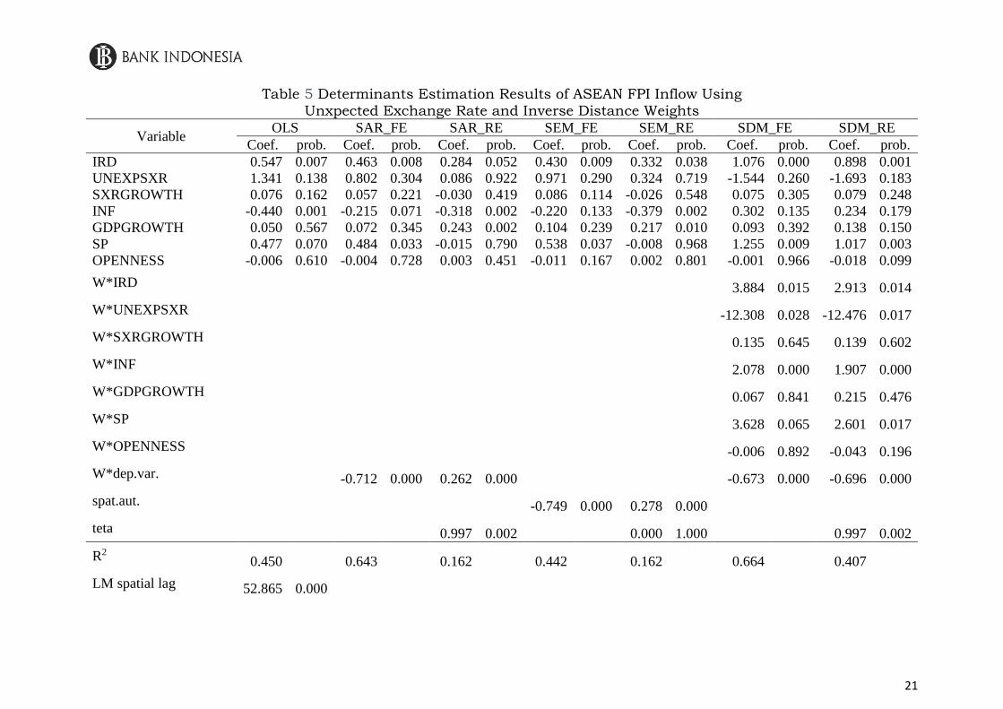
Table 5 Determinants Estimation Results of ASEAN FPI Inflow Using Unxpected Exchange Rate and Inverse Distance Weights

Variable OLS SAR_FE SAR_RE SEM_FE SEM_RE SDM_FE SDM_RE

Coef. prob. Coef. prob. Coef. prob. Coef. prob. Coef. prob. Coef. prob. Coef. prob.

IRD 0.547 0.007 0.463 0.008 0.284 0.052 0.430 0.009 0.332 0.038 1.076 0.000 0.898 0.001

UNEXPSXR 1.341 0.138 0.802 0.304 0.086 0.922 0.971 0.290 0.324 0.719 -1.544 0.260 -1.693 0.183

SXRGROWTH 0.076 0.162 0.057 0.221 -0.030 0.419 0.086 0.114 -0.026 0.548 0.075 0.305 0.079 0.248

INF -0.440 0.001 -0.215 0.071 -0.318 0.002 -0.220 0.133 -0.379 0.002 0.302 0.135 0.234 0.179

GDPGROWTH 0.050 0.567 0.072 0.345 0.243 0.002 0.104 0.239 0.217 0.010 0.093 0.392 0.138 0.150

SP 0.477 0.070 0.484 0.033 -0.015 0.790 0.538 0.037 -0.008 0.968 1.255 0.009 1.017 0.003

OPENNESS -0.006 0.610 -0.004 0.728 0.003 0.451 -0.011 0.167 0.002 0.801 -0.001 0.966 -0.018 0.099

W*IRD 3.884 0.015 2.913 0.014

W*UNEXPSXR -12.308 0.028 -12.476 0.017

W*SXRGROWTH 0.135 0.645 0.139 0.602

W*INF 2.078 0.000 1.907 0.000

W*GDPGROWTH 0.067 0.841 0.215 0.476

W*SP 3.628 0.065 2.601 0.017

W*OPENNESS -0.006 0.892 -0.043 0.196

W*dep.var. -0.712 0.000 0.262 0.000

-0.673 0.000 -0.696 0.000

spat.aut. -0.749 0.000 0.278 0.000

teta 0.997 0.002

0.000 1.000

0.997 0.002

R2 0.450

0.643

0.162

0.442

0.162

0.664

0.407

LM spatial lag 52.865 0.000

22

LM spatial error 50.983 0.000

Robust LM spatial lag 3.182 0.074

Robust LM spatial error 1.300 0.254

Wald test spatial lag 23.085 0.002 24.162 0.001

LR test spatial lag 24.137 0.001 24.018 0.001

Wald test spatial error 22.020 0.003 22.623 0.002

LR test spatial error 12.777 0.078 21.250 0.003

Hausman Test (Prob.) 2896.5953 (0.0000) -591.7256 (0.0000) 7.7790 (0.9323)

23

The spatial relationship between the macroeconomic variables of the neighboring

countries and the inflow of the host country's FPI, or vice versa is analyzed in Sub-chapter 4.5.

This is because the estimation analysis of the spatial relationship between the macroeconomic

variables of the neighboring countries and the host country's FPI inflows using the SDM

estimation results may produce bias conclusions. According to Elhorst (2014), the indirect

(spillover) effect needs to be used in testing the presence of a spatial spillover effect, compared

to the estimated coefficient in the spatial durbin (SDM) model. Indirect effects refer to the

influence of factors in the host country on the surrounding region. Additionally, the direct effect

on SDM is also tested due to the existence of feedback effects on the independent variable of

the host on the inflow its FPI. According to Li & Li (2020), the direct effect is important to

estimate because it includes two types of effects, namely (1) changes in the independent

variable of the host country directly led to changes in the dependent variable of the host

country; (2) changes in the independent variable of the host country cause changes in the

dependent variable in the surrounding area, and changes in the surrounding area in turn affect

the area of the host, thus forming a feedback effect. The direct and indirect effects differ from

the SDM estimation results because these effects are calculated by a complex mathematical

formula. Their dispersion depends on all estimated coefficients involved (Elhorst, 2014b).

For the robustness test, we compared the estimation results of SDM with SAR and SEM

using inverse distance weights. The result is the same as SDM. The estimation results of the

SAR and SEM models with spatial fixed effects and time periods (SAR-FE and SEM-FE) for

Model 1 can be seen in Table 6 column 2 and Table 6 column 4. Similar with SDM, the

estimation results of the SAR-FE model show the coefficient ρ significant 1% with a negative

sign, which means that an increase in FPI inflows to neighboring countries will reduce FPI

inflows to host countries for the case of the ASEAN Region. The estimation results of the SAR

and SEM models also show that FPI inflows are significantly affected by the interest rate

differential and government debt ratings at the significant levels of 1% and 5%. Likewise, the

SEM-FE model shows the results of the coefficient λ which are negative, which means that the

error-term in neighboring countries has a negative effect on FPI flows into the host country.

4.2.2 Relationship of Expected Exchange Rate and Several Macroeconomic Variables




model, including being significant and negative. This indicates that an increase in the inflow

of FPI to neighboring countries reduces the inflow of FPI to the host country. According to

Table 6 column 7, the estimation results of the relationship between the macroeconomic

variables of the host country and its flow of FPI are the same as in Model 1. Specifically, only

the interest rate differential variable and the government debt rating of the host country have a

significant positive effect on FPI inflows to the host country at the significance level of 1%.

For the Model 2 robustness test, we compared the estimation results of SDM with SAR

and SEM using inverse distance weights. The result is the same as SDM. The estimation results

of the SAR and SEM models with spatial fixed effects and time periods (SAR-FE and SEM-

FE) for Model 2 can be seen in Table 6 column 2 and Table 6 column 4. Similiar with SDM,

the estimation results of the SAR-FE model show the coefficient ρ significant 1% with a

negative sign. The estimation results of the SAR and SEM models also show that FPI inflows

are significantly affected by the interest rate differential and government debt ratings at the

significant levels of 1% and 5%. Likewise, the SEM-FE model shows the results of the

coefficient λ which are negative, which means that the error-term in neighboring countries has

a negative effect on FPI flows into the host country.

24

Table 6 Determinants Estimation Results of ASEAN FPI Inflow Using Expected Exchange Rate and Inverse Distance Weights



IRD 0.637 0.001 0.518 0.002 0.342 0.014 0.476 0.003 0.395 0.010 1.072 0.000 0.910 0.001

EXPSXR 0.003 0.769 0.001 0.882 -0.009 0.334 0.002 0.834 -0.009 0.345 -0.013 0.487 -0.020 0.198

SXRGROWTH 0.055 0.295 0.044 0.331 -0.033 0.365 0.071 0.181 -0.033 0.445 0.067 0.348 0.070 0.294

INF -0.414 0.003 -0.196 0.099 -0.312 0.003 -0.193 0.186 -0.369 0.003 0.292 0.146 0.254 0.145

GDPGROWTH 0.060 0.496 0.078 0.305 0.231 0.004 0.109 0.220 0.213 0.011 0.089 0.413 0.137 0.159

SP 0.462 0.083 0.473 0.039 -0.010 0.866 0.533 0.039 -0.023 0.914 1.265 0.010 0.935 0.007

OPENNESS -0.007 0.600 -0.004 0.721 0.003 0.409 -0.010 0.199 0.002 0.717 -0.001 0.975 -0.015 0.173

W*IRD 3.662 0.025 2.899 0.017

W*EXPSXR -0.092 0.228 -0.116 0.084

W*SXRGROWTH 0.105 0.722 0.122 0.651

W*INF 2.092 0.001 2.017 0.000

W*GDPGROWTH 0.063 0.852 0.210 0.492

W*SP 3.916 0.055 2.436 0.026

W*OPENNESS 0.003 0.944 -0.036 0.285

W*dep.var. -0.717 0.000 0.260 0.000

-0.666 0.000 -0.687 0.000

spat.aut. -0.759 0.000 0.271 0.000

teta 0.997 0.002

0.000 1.000

0.997 0.002

R2 0.447

0.645

0.164

0.438

0.163

0.659

0.398


25









26

4.3 Estimation Results on the Relationship of Exchange Rate Volatility and Several

Macroeconomic Variables to FPI Inflows with 1-order binary contiguity





model, including being significant and negative. The SDM results using binary contiguity

weighting in Model 3 show that the results of the estimation of the effect of the interest rate

differential and the host country's government debt rating on FPI flows into the host country

are the same as Models 1 and 2, which are positive and significant. Furthermore, exchange rate

volatility and changes, as well as host country economic growth insignificantly affect FPI

inflows. However, inflation and trade openness in the host country have a significant negative

effect on FPI flows into the host country at the significant levels of 1% and 5%. The negative

relationship between inflation and FPI inflows was also reported by Waqas et al. (2015) in

China and India, as well as Al-Smadi (2018) in Jordan. The higher the inflation in the host

country, the lower the real interest rate. This reduces the return of foreign portfolio investors,

making them hold their funds to invest in the host country.

Trade openness and FPI inflows have a significant negative relationship. This is in line

with Ahmed Hannan (2017), which established a negative relationship between trade openness

and FPI. Similarly, Marouane (2019) found a negative relationship between trade openness and

FDI. According to Ahmed Hannan (2017), the negative relationship is attributed to the

influence of the selection of the period used and not a representative of the expected

relationship between capital flows and trade openness. Furthermore, the impact of trade

openness may not be captured accurately because indicators, such as disclosure of capital

reports, are slow-moving. Coupled with the robustness test using the expected exchange rate

as an independent variable, where the fixed effect is selected compared to the random effect in

the spatial durbin model. In this regard, the trade openness variable does not significantly affect

the FPI inflow. According to Alwafi (2017), the open trade of a country negatively impacts the

economy in developing countries that specialize in low-quality export products (primary

consumer products), which are vulnerable to trade shocks.

27

Table 7 Determinants Estimation Results of ASEAN FPI Inflow Using Unexpected Exchange Rate and Weights of 1-order binary contiguity



IRD 0.547 0.007 0.521 0.009 0.271 0.071 0.431 0.007 0.248 0.131 0.629 0.006 0.587 0.001

UNEXPSXR 1.341 0.138 1.086 0.225 0.016 0.986 1.270 0.163 0.021 0.982 1.040 0.248 1.285 0.122

SXRGROWTH 0.076 0.162 0.059 0.269 -0.044 0.243 0.082 0.131 -0.035 0.401 0.056 0.283 0.077 0.108

INF -0.440 0.001 -0.330 0.015 -0.313 0.004 -0.331 0.017 -0.364 0.002 -0.403 0.003 -0.428 0.001

GDPGROWTH 0.050 0.567 0.124 0.153 0.282 0.000 0.122 0.162 0.264 0.002 0.154 0.072 0.141 0.073

SP 0.477 0.070 0.643 0.013 -0.006 0.920 0.450 0.050 -0.181 0.382 0.860 0.002 0.614 0.007

OPENNESS -0.006 0.610 -0.011 0.382 0.002 0.565 -0.009 0.179 0.007 0.264 -0.011 0.385 -0.013 0.042

W*IRD -0.917 0.119 0.279 0.321

W*UNEXPSXR -0.464 0.809 -0.944 0.560

W*SXRGROWTH 0.114 0.082 0.074 0.197

W*INF -0.554 0.033 -0.311 0.180

W*GDPGROWTH 0.860 0.000 0.743 0.000

W*SP -0.825 0.269 -0.257 0.145

W*OPENNESS -0.030 0.179 0.004 0.778

W*dep.var. -0.193 0.000 0.107 0.036

-0.244 0.000 -0.270 0.000

spat.aut. -0.270 0.000 0.110 0.034

teta 0.997 0.002

0.000 1.000

0.997 0.002

R2 0.450

0.532

0.107

0.446

0.107

0.589

0.286


28








Hausman Test (Prob.) 360.1277 (0.0000) 326.2535 (0.0000) 22.0751 (0.1059)

29

By comparing the estimation results of SDM with SAR and SEM we conducted a

robustness test in Model 3. The results were the same as SDM, except for the trade openness

variable, which did not significantly affect the FPI inflow to ASEAN. The estimation results

of the SAR and SEM models with spatial fixed effects and time periods (SAR-FE and SEM-

FE) for Model 3 can be seen in Table 7 column 2 and Table 7 column 4. Similiar with SDM,

the estimation results of the SAR-FE model show the coefficient ρ 1% significant with a

negative sign. The estimation results of the SAR and SEM models also show that FPI inflows

are significantly affected by the interest rate differential, inflation and government debt ratings

at the significant level of 1% -5%. Likewise, the SEM-FE model shows the results of the



4.3.2 Relationship of Expected Exchange Rate and Several Macroeconomic Variables to

FPI Inflow in ASEAN

Based on Hausman test, fixef effect is selected for the SDM model (SDM-FE) for Model

4. The coefficient ρ generated in the SDM-FE estimation is the same as the SAR-FE model,

which is significant and negative. According to Table 8 column 6, the estimation results of the

macroeconomic variable relationship between the host country and its FPI inflows are the same

as Model 3, where the interest rate differential, inflation, and host country government debt

ratings significantly affect the FPI flows into the host country at the significant level of 1%,

except for the trade openness variable that not significant.

By comparing the estimation results of SDM with SAR and SEM, we conducted a

robustness test on Model 4. The results were the same as SDM. The estimation results of the

SAR and SEM models with spatial fixed effects and time periods (SAR-FE and SEM-FE) for

Model 4 can be seen in Table 8 column 2 and Table 8 column 4. Similar with SDM, the

estimation results of the SAR-FE model show the coefficient ρ significant 1% with a negative

sign. The estimation results of the SAR and SEM models also show that FPI inflows are

significantly affected by the interest rate differential, inflation and government debt ratings at

the significant level of 1% -5%. Likewise, the SEM-FE model shows the results of the



30

Table 8 Estimation Results of Determinants for FPI Inflow in ASEAN Using the Expected Exchange Rate and Weights of 1-order binary contiguity



IRD 0.637 0.001 0.560 0.003 0.343 0.017 0.469 0.002 0.323 0.040 0.644 0.004 0.637 0.000

EXPSXR 0.003 0.769 0.013 0.229 -0.013 0.190 0.011 0.311 -0.014 0.155 0.013 0.221 0.015 0.138

SXRGROWTH 0.055 0.295 0.051 0.329 -0.046 0.211 0.071 0.183 -0.038 0.357 0.059 0.246 0.074 0.117

INF -0.414 0.003 -0.325 0.017 -0.302 0.005 -0.319 0.022 -0.354 0.003 -0.384 0.005 -0.427 0.001

GDPGROWTH 0.060 0.496 0.125 0.150 0.262 0.001 0.126 0.149 0.247 0.003 0.154 0.072 0.134 0.089

SP 0.462 0.083 0.678 0.010 0.002 0.979 0.461 0.046 -0.190 0.359 0.841 0.002 0.639 0.005

OPENNESS -0.007 0.600 -0.010 0.398 0.003 0.506 -0.009 0.183 0.008 0.212 -0.010 0.404 -0.013 0.042

W*IRD -1.143 0.047 0.137 0.617

W*EXPSXR 0.025 0.243 0.016 0.413

W*SXRGROWTH 0.090 0.171 0.058 0.324

W*INF -0.548 0.043 -0.330 0.176

W*GDPGROWTH 0.873 0.000 0.737 0.000

W*SP -0.572 0.432 -0.403 0.020

W*OPENNESS -0.021 0.337 0.015 0.313

W*dep.var. -0.204 0.000 0.114 0.025

-0.252 0.000 -0.274 0.000

spat.aut. -0.278 0.000 0.111 0.031

teta 0.997 0.002

0.000 1.000

0.997 0.002

R2 0.447

0.534

0.112

0.440

0.113

0.592

0.284


31








Hausman Test (Prob.) 427.9590 (0.0000) 290.7662 (0.0000) 25.3352 (0.0456)

32

4.4 Estimation Results on the Relationship of Exchange Rate Volatility and Several

Macroeconomic Variables to FPI Inflows with Economic Distance





including being significant and negative. The SDM results using economic distance weighting

in Model 5 show that the results of the estimation of the effect of the interest rate differential

and the host country's government debt rating on FPI flows into the host country are the same

as Models 1-4, which are positive and significant. Furthermore, exchange rate volatility and

changes, as well as host country economic growth insignificantly affect FPI inflows. However,

inflation, economic growth, and trade openness in the host country have a significant effect on

FPI flows into the host country at the significant levels of 1%. The negative relationship

between inflation and FPI inflows was also reported by Waqas et al. (2015) in China and India,

as well as Al-Smadi (2018) in Jordan. The higher the inflation in the host country, the lower

the real interest rate. This reduces the return of foreign portfolio investors, making them hold

their funds to invest in the host country. The estimation results show a negative relationship

between inflation and trade openness with FPI inflows and also a positive relationship between

economic growth and FPI inflows. This result is different from the research hypothesis where

openness of host trade has a positive impact on FPI inflows. We found no systematic evidence

of a negative relationship between trade openness and FPI inflows. However, according to

Fratzscher (2012), there are several indications that the more open a country's finances can lead

to greater capital outflows.

By comparing the estimation results of SDM with SAR and SEM we perform

robustness tests on Model 5. The results are similar to SDM, except for the variables of trade

openness and economic growth, where trade openness of the host country significantly affects

the inflow of FPI to ASEAN in SEM, but not significant impact on SAR and the economic

growth of host countries did not significantly affect FPI inflows to ASEAN in SAR and SEM.

The estimation results of the SAR and SEM models with spatial fixed effects and time periods

(SAR-FE and SEM-FE) for Model 5 can be seen in Table 9 column 2 and Table 9 column 4.

The estimation results of the SAR-FE model show a significant coefficient of 1%. with a

negative sign. The estimation results of the SAR model show that FPI inflows are significantly

influenced by the interest rate differential, inflation and government debt ratings at the

significant level of 1% -5%, while in SEM, interest rate differential, inflation, government bond

ratings, and trade openness host countries influence FPI inflows. In addition, the SEM-FE

model shows the results of the coefficient λ which are negative, which means that the error-

term in neighboring countries has a negative effect on FPI flows into the host country.

4.4.2 Relationship of Expected Exchange Rate and Several Macroeconomic Variables on

FPI Inflows in ASEAN



including being significant and negative. Based on Table 10 column 6, the estimation results

of the macroeconomic variable relationship between the host country and the host country's

FPI inflows are the same as Model 5, where the variable interest rate differential, inflation,

economic growth, government debt rating, and trade openness of the host country are

significant on FPI flows into the host country at the 1-5% significant level.

33

By comparing the estimation results of SDM with SAR and SEM we perform robustness

tests on Model 6. The results are similar to SDM, except for the variables of trade openness

and economic growth, where trade openness of the host country significantly affects the flow

of FPI to ASEAN in SEM, but not significant impact on SAR and the economic growth of host

countries did not significantly affect FPI inflows to ASEAN in SAR and SEM. The estimation

results of the SAR and SEM models with spatial fixed effects and time periods (SAR-FE and

SEM-FE) for Model 6 can be seen in Table 10 column 2 and Table 10 column 4. The estimation

results of the SAR-FE model show a significant coefficient of 1% with a negative sign. The

estimation results of the SAR model show that FPI inflows are significantly influenced by the

interest rate differential, inflation and government debt ratings at the significant level of 1% -

5%, while in SEM, interest rate differential, inflation, government bond ratings, and trade

openness host countries influence FPI inflows. In addition, the SEM-FE model shows the

results of the coefficient λ which are negative, which means that the error-term in neighboring

countries has a negative effect on FPI flows into the host country.

34

Table 9 Estimation Results of Determinants for FPI Inflow in ASEAN Using the Unexpected Exchange Rate and Weights of economic distance



IRD 0.547 0.007 0.591 0.005 0.285 0.053 0.612 0.001 0.345 0.034 0.993 0.000 0.972 0.000

UNEXPSXR 1.341 0.138 1.236 0.187 0.101 0.910 1.441 0.162 0.320 0.723 1.594 0.227 1.559 0.172

SXRGROWTH 0.076 0.162 0.068 0.226 -0.039 0.290 0.086 0.161 -0.024 0.578 0.033 0.639 0.050 0.433

INF -0.440 0.001 -0.412 0.004 -0.338 0.001 -0.431 0.005 -0.406 0.001 -0.408 0.020 -0.411 0.007

GDPGROWTH 0.050 0.567 0.093 0.309 0.284 0.000 0.167 0.070 0.260 0.002 0.334 0.002 0.325 0.000

SP 0.477 0.070 0.580 0.034 -0.025 0.673 0.714 0.011 -0.066 0.761 1.521 0.000 1.422 0.000

OPENNESS -0.006 0.610 -0.008 0.552 0.003 0.440 -0.017 0.046 0.004 0.562 -0.040 0.012 -0.038 0.000

W*IRD 1.380 0.050 1.456 0.004

W*UNEXPSXR 0.069 0.978 0.103 0.964

W*SXRGROWTH -0.144 0.340 -0.130 0.339

W*INF 0.015 0.972 -0.063 0.867

W*GDPGROWTH 1.642 0.000 1.485 0.000

W*SP 2.751 0.001 2.733 0.000

W*OPENNESS -0.048 0.491 -0.020 0.583

W*dep.var. -0.262 0.000 0.280 0.000

-0.324 0.000 -0.435 0.000

spat.aut. -0.503 0.000 0.272 0.000

teta 0.997 0.002

0.000 1.000

0.997 0.002

R-squared 0.450 0.495

0.146

0.441

0.563

0.278


35









36

4.5 Direct Effects and Spillover Effects of Several Macroeconomic Variables on FPI

Inflows in ASEAN

For robustness testing, analysis of direct effects and indirect effects has been carried out

to detect feedback effect and spillover effect between neighboring countries and the host

country. The direct effect estimate from Model 1 is significant and positive for the interest rate

differential variable with a significant level of 5% and a government debt rating with a

significant level of 10%, which is considered statistically less robust. The elasticity value of

the interest rate differential is 0.441. The estimated direct effect differs from the estimated

SDM-RE coefficient of 0.898 which is shown in Table 5 column (7). This difference is due to

the feedback effect that arises as a result of the impact of passing the dependent variable to a

neighboring country based on the nonzero element in the matrix W and returning to that country

(Jing et al., 2017).

According to Elhorst (2014a), the cause of this feedback effect is partly due to the

coefficient of the spatially lagged dependent variable (𝜌), the result of which is negative and

significant and partly due to the coefficient of the spatially lagged value of the independent

variable itself (𝜃𝑘). Since the direct effect of the interest rate differential variable is 0.441 and

the estimated coefficient is 0.898, the feedback effect is -0.457. In other words, this feedback

effect turns out to be relatively large. The negative value of this feedback effect indicates that

an increase in the interest rate differential to the host country reduces the impact of increased

FPI inflows to the host country as a result of the impact of passing through neighboring

countries and returning to the state itself.

When compared with the results of SDM estimates, where empirical evidence is found

that the spatial lag coefficient of the independent variables is more supportive of the

interference relationship between the independent variables of the host country and the influx

of FPI in neighboring countries compared to the indirect effect seen from the significance of

each independent variable. This is probably because the calculation of the indirect effect

(spillover) depends on three parameters (𝜌, 𝛽𝑘, 𝜃𝑘), so that if one of the three parameters is not

significant, then there is a possibility that the indirect effect becomes insignificant (Jing et al.,

2017). The estimated spillover (indirect) effect in Model 1 is that inflation is only significant

and positive at the 5% significant level. The spillover effect in Model 1 shows that an increase

in inflation in the host country to some extent can increase the inflow of FPI in neighboring

countries with an elasticity of 1.383.

37

Table 10 Estimation Results of Determinants for FPI Inflow in ASEAN Using the Expected Exchange Rate and Weights of economic distance



IRD 0.637 0.001 0.665 0.001 0.361 0.010 0.675 0.000 0.431 0.006 1.063 0.000 1.031 0.000

EXPSXR 0.003 0.769 0.005 0.635 -0.012 0.200 0.008 0.527 -0.013 0.187 0.015 0.337 0.013 0.299

SXRGROWTH 0.055 0.295 0.051 0.348 -0.043 0.234 0.071 0.241 -0.032 0.452 0.027 0.704 0.044 0.486

INF -0.414 0.003 -0.389 0.006 -0.331 0.002 -0.406 0.008 -0.389 0.002 -0.380 0.029 -0.387 0.011

GDPGROWTH 0.060 0.496 0.099 0.277 0.269 0.001 0.171 0.065 0.253 0.002 0.313 0.004 0.308 0.001

SP 0.462 0.083 0.578 0.036 -0.017 0.774 0.733 0.009 -0.086 0.690 1.588 0.000 1.478 0.000

OPENNESS -0.007 0.600 -0.008 0.549 0.003 0.390 -0.017 0.048 0.005 0.467 -0.040 0.013 -0.039 0.000

W*IRD 1.336 0.046 1.418 0.003

W*EXPSXR 0.026 0.357 0.026 0.303

W*SXRGROWTH -0.093 0.530 -0.081 0.539

W*INF 0.029 0.948 -0.054 0.887

W*GDPGROWTH 1.496 0.000 1.344 0.000

W*SP 2.984 0.000 2.976 0.000

W*OPENNESS -0.045 0.508 -0.023 0.534

W*dep.var. -0.274 0.000 0.273 0.000

-0.335 0.000 -0.444 0.000

spat.aut. -0.511 0.000 0.265 0.000

teta 0.997 0.002

0.000 1.000

0.997 0.002

R-squared 0.447

0.494

0.148

0.436

0.562

0.274


38









39

The estimated direct effects of Model 2 are the same as those of Model 1, where only the

interest rate differential variable of the host country has a significant positive effect at the 5%

significance level. In the SDM-RE model, the interest rate differential and government debt

securities of the host country have a significant effect on the 5% significant level. Furthermore,

the feedback effect of interest rate differential is relatively large, with a value of -0.382. The

estimated spillover effect (indirect) in Model 2 is that inflation is only significant and positive

at the significant level of 1%, with an elasticity of 1.434.

In the estimation of the direct effects of Model 3, the variable interest rate differential,

inflation, and government debt rating have a significant effect at the 5% level. This suggests

that an increase in the difference in bond interest rates between the host country and the United

States, as well as an increase in the government debt rating increase foreign portfolio inflows

in the host country, with elasticities of 0.570 and 0.667. Meanwhile, an increase in host country

inflation will reduce the inflow of the host country's FPI with an elasticity of -0.405. The

feedback effect of variable interest rate differential, inflation, and government debt ratings is

relatively small, amounting to -0.017, -0.022, and 0.053. The negative value of the feedback

effect on this variable interest rate differential and inflation shows that an increase in the interest

rate differential and inflation to the host country reduces the impact of increased FPI inflows

to the host country as a result of the impact of passing through neighboring countries and

returning to the state itself. Meanwhile, the positive value of the feedback effect on the

government debt rating variable shows that an increase in the rating of government debt

securities to the host country has an impact on increasing the impact of increased FPI inflows

to the host country as a result of the impact of passing through neighboring countries and

returning to the state itself.

The estimated spillover (indirect) effect in Model 3 is only significant and positive

economic growth, which is the same as the SDM-RE estimate. The spillover effect in Model 3

shows that increased growth in the host country to some extent can increase the FPI inflows in

neighboring countries with an elasticity of 0.646. This shows that if the host country

experiences an increase in economic growth, it will indirectly have a positive impact on FPI

inflows in neighboring countries. This is because investors think that increased economic

growth in the host country will increase the economic growth of neighboring countries.

In the estimation of the direct effect of Model 4, the variable interest rate differential and

government debt rating have a significant effect with elasticities of 0.797 and 0.932. The

feedback effect of the variable interest rate differential and government debt ratings is relatively

small, amounting to 0.153 and 0.091. The spillover effect estimate (indirect) in Model 4 is only

significant and positive economic growth, which is the same as the SDM-RE estimate. The

spillover effect in Model 4 shows that increasing growth in the host country to some extent can

increase the inflow of FPI in neighboring countries with an elasticity of 0.760.

In the estimation of the direct effects of Model 5, variable interest rate differential,

inflation, government debt rating, and trade openness have a significant effect with elasticities

of 0.899, -0.424, 1.321, and -0.038. The feedback effect of variable interest rate differential,

inflation, government debt rating, and trade openness is relatively small, amounting to 0.094, -

0.016, 0.199, and 0.002. The estimated spillover effect (indirect) in Model 5 is that economic

growth and the government debt rating are significant and positive. The spillover effect in

Model 5 shows that an increase in economic growth and a government debt rating in the host

country can to some extent increase the inflow of FPI in neighboring countries with elasticities

of 1.307 and 1.931.

Similiar with Model 5, in the estimation of the direct effects of Model 6, variable interest

rate differential, inflation, government debt ratings, and trade openness have a significant effect

40

with elasticities of 0.970, -0.398, 1.362, and -0.037. The feedback effects of variable interest

rate differential, inflation, government debt ratings, and trade openness are relatively small,

amounting to 0.093, -0.018, 0.225, and 0.002. The estimated spillover effect (indirect) in Model

6 is that the economic growth and government debt rating are significant and positive. The

spillover effect in Model 6 shows that an increase in economic growth and a government debt

rating in the host country can to some extent increase the inflows of FPI in neighboring

countries with elasticities of 1.175 and 2.094.

41

Table 11 Direct and Spillover Effects

Model 1 Model 2 Model 3 Model 4 Model 5 Model 6

Coef. prob. Coef. prob. Coef. prob. Coef. prob. Coef. prob. Coef. prob.

Direct Effects IRD 0.441 0.038 0.528 0.022 0.570 0.019 0.797 0.015 0.899 0.012 0.970 0.007

UNEXPSXR/EXPSXR 0.527 0.553 -0.003 0.790 1.421 0.123 0.010 0.389 1.638 0.232 0.013 0.408

SXRGROWTH 0.063 0.245 0.055 0.320 0.069 0.228 0.047 0.410 0.046 0.523 0.034 0.617

INF -0.110 0.465 -0.061 0.669 -0.405 0.023 -0.332 0.056 -0.424 0.040 -0.398 0.057

GDPGROWTH 0.113 0.197 0.118 0.203 0.053 0.555 0.060 0.508 0.194 0.105 0.176 0.132

SP 0.632 0.051 0.631 0.052 0.667 0.039 0.932 0.035 1.321 0.013 1.362 0.013

OPENNESS -0.011 0.193 -0.010 0.246 -0.014 0.093 -0.008 0.577 -0.038 0.049 -0.037 0.049

Indirect Effects IRD 1.815 0.076 1.800 0.068 0.125 0.626 -1.199 0.063 0.890 0.186 0.830 0.176

UNEXPSXR/EXPSXR -8.989 0.059 -0.078 0.142 -1.121 0.471 0.020 0.352 -0.409 0.837 0.020 0.399

SXRGROWTH 0.063 0.745 0.044 0.815 0.051 0.378 0.070 0.320 -0.137 0.306 -0.092 0.458

INF 1.383 0.012 1.434 0.009 -0.189 0.392 -0.417 0.150 0.132 0.722 0.119 0.740

GDPGROWTH 0.099 0.644 0.092 0.674 0.646 0.006 0.760 0.005 1.307 0.008 1.175 0.012

SP 1.530 0.088 1.371 0.111 -0.394 0.084 -0.721 0.340 1.931 0.036 2.094 0.026

OPENNESS -0.025 0.296 -0.019 0.428 0.008 0.608 -0.017 0.443 -0.029 0.634 -0.027 0.656

Total Effects IRD 2.257 0.044 2.328 0.037 0.695 0.075 -0.402 0.484 1.789 0.048 1.800 0.032

UNEXPSXR/EXPSXR -8.462 0.078 -0.081 0.154 0.300 0.858 0.030 0.195 1.229 0.668 0.033 0.345

SXRGROWTH 0.126 0.533 0.099 0.631 0.120 0.100 0.118 0.133 -0.091 0.595 -0.058 0.720

INF 1.273 0.028 1.373 0.019 -0.594 0.047 -0.749 0.039 -0.291 0.537 -0.278 0.543

42

GDPGROWTH 0.212 0.377 0.210 0.401 0.700 0.005 0.821 0.004 1.501 0.008 1.351 0.011

SP 2.161 0.050 2.002 0.065 0.273 0.265 0.211 0.722 3.252 0.015 3.456 0.012

OPENNESS -0.037 0.207 -0.029 0.323 -0.006 0.664 -0.025 0.274 -0.067 0.319 -0.064 0.333

43

There is evidence that when using the inverse distance matrix as a spatial weight, the

resulting feedback effect is relatively large. Meanwhile, when using a 1-order binary contiguity

matrix as a spatial weight, the resulting feedback effect is relatively small. Based on research

using the spatial durbin model conducted by Elhorst (2014a), by using the weight of a 1-order

binary contiguity matrix, the feedback effect is relatively small. This is probably because the

use of inverse distance weight makes neighboring countries have a value from the distance

between capital cities, hence the effect of passing through neighboring countries and returning

to the country is greater. Meanwhile, the weight using 1-order binary contiguity makes only

countries that share state boundaries have a spatial impact. Therefore, the effect of passing

through neighboring countries and returning to the country is smaller. When considering spatial

correlation based on economy (economic distance), the results of the spillover effect show

more linkages between the macroeconomic variables of the host country and changes in FPI

flows into neighboring countries, when compared to using geographic correlation. This is more

understandable because investors consider the economic linkages between neighboring

countries more than the geographical linkages to invest in a country.

4.6 The Relationship of Unexpected Exchange Rate and Several Macroeconomic

Variables to FPI Inflow in Indonesia

The foreign portfolio is divided into three, including net foreign inflows of equity

(EQUITY), 10-year government bonds (BOND), and FPI (bonds plus equity). Augmented

Dickey-Fuller (ADF) test shows that the foreign capital inflows in all types of portfolios,

changes in exchange rates and volatility, VIX index. The interest rate differential is stationary

at I (0), as shown in Table 12. Since all variables are stationary at the level, the OLS ARMA

model is estimated. Importantly, the best model is selected by considering the significance of

various estimation models from the statistical probability of F-test, the significance of AR or

MA coefficients used, the maximum value of log-likelihood function, and the minimum value

of AIC and SIC criteria.

First, we estimate a linear model, in which the net inflows of equity (equity), bonds, and

FPI (bonds plus equity) are the dependent variables on the OLS standard setting, which is

shown in Table 14. In the OLS model, ARMA (2,0) is selected for equity and bonds, and

ARMA (2,1) for FPI as the best model. The results indicate that changes in the exchange rate

and VIX index in the previous period have a significant negative effect on bonds and FPI, yet

not significant on equity. Exchange rate volatility (UNEXPSXR)1 in the past period

significantly affected foreign equity inflows to Indonesia only. Meanwhile, the interest rate

differential in the previous period has a statistically significant positive effect on bonds and

FPI and not significant on equity. To test the robustness of the model, serial correlation and

heteroscedasticity tests were conducted in the ARCH effect test for all types of portfolios. The

result shows that there is no serial correlation in the model, though there is heteroscedasticity

in the ARCH effect test. This shows that a simple linear model is not suitable for capturing the

relationship between exchange rates and macroeconomic variables on net inflows of foreign

portfolio investment. Therefore, the ARCH-GARCH method is used for estimation.

Table 12 Augmented Dickey-Fuller (ADF) Stationarity Test at Level

Variable t-Statistic Prob.*

BOND -23.660 0.000

EQUITY -27.782 0.000

FPI -23.158 0.000

1 We have also tried using the expected exchange rate data, but the results are negative and insignificant with a

very small coefficient.

44

SXRGROWTH -2.182 0.028

UNEXPSXR -4.572 0.000

VIX -5.846 0.000

IRD -3.487 0.008

Furthermore, the ARCH-GARCH method produced a better estimate as indicated by the

absence of heteroscedasticity in the ARCH effect test and the significant impact of ARCH and

GARCH parameters in all cases, as shown in Table 14. GARCH (1,1) was selected as the best

model in all types of portfolios. The results show that in all types of portfolios, changes in

exchange rates on the previous day (for bonds and FPI) and two days before (for equity) have

a significant negative effect. In case the rupiah depreciates (appreciates), foreign investors tend

to sell Indonesian portfolios and bonds. This is in line with Anggitawati & Ekaputra (2018) ,

which examined the exchange rate changes to portfolios in Indonesia in 2011–2016 using the

VAR method.

According to Anggitawati & Ekaputra (2018), the impact of negative shocks from

changes in exchange rates on net flows in the capital, bond, and equity markets occurs on the

second to fourth trading days. Srinivasan & Kalaivani (2015) reported that the exchange rate

has a significant negative impact on Foreign Institutional Investment (FII) in India. According

to Hau & Rey (2002), there is a negative correlation between the exchange rate and foreign

stock market returns, reducing the volatility in exchange rate returns. For this reason, foreign

investors are more interested. Furthermore, the negative correlation is also related to the

findings of this study. There is an increase in returns or changes in exchange rates, which

decreases stock returns. For this reason, foreign investors withdraw their capital, leading to the

outflow of foreign portfolio investment.

Table 13 Linear Model Estimation

Variable

BOND EQUITY FPI

Coef. Prob. Coef. Prob. Coef. Prob.

C 0.627 0.061 -0.453 0.416 0.249 0.532

SXRGROWTH(-1) -0.016 0.014

-0.016 0.019

SXRGROWTH(-2)

-0.004 0.548

UNEXPSXR(-1) -0.127 0.422 -0.453 0.045 -0.305 0.078

VIX(-1)

-0.038 0.000

VIX(-2) -0.053 0.000 0.008 0.421

IRD(-1)

0.108 0.311

IRD(-2)

IRD(-3) 0.146 0.027

0.175 0.026

AR(1) 0.273 0.001 0.195 0.030 0.275 0.000

AR(2) 0.185 0.000 0.129 0.000 0.199 0.000

R2 0.182

0.069

0.184

Adj R2 0.180

0.067

0.182

LogL -4544.372

-5807.088

-4630.147

45

AIC 3.509

4.481

3.575

SIC 3.525

4.497

3.591

Serial Correlation

Test 1.239 0.290 0.836 0.433 1.488 0.223

Heteroskedasticity

Test 611.243 0.000 11.458 0.001 142.254 0.000

Note: Serial Correlation Test using the Breusch-Godfrey Serial Correlation LM Test and Heteroscedasticity Test using the ARCH LM Test.

There is a negative and significant relationship between exchange rate volatility

(UNEXPSXR) in the previous one-day period on the equity market and the foreign portfolio

market (FPI) but not significant in bond positions. This means that the higher exchange rate

volatility in Indonesia attracts foreign equity and portfolio outflow. This is in line with Garg &

Dua (2014), which showed a negative relationship between exchange rate volatility and foreign

portfolio inflows because of the higher level of uncertainty in the returns received by investors.

Persson & Svensson (1989) showed that the characteristics of risk through exchange rate

variability determines the composition of international portfolios and asset trading due to

incomplete international asset markets. This contravenes Baek (2006), which showed that real

exchange rate volatility does not significantly affect foreign portfolio investment inflows

because the domestic factors in the Asian and Latin American regions do not affect the FPI

inflows. Additionally, factors from outside the host country are more influential on FPI in Asia

and Latin America.

This is shown by the significant VIX index in previous periods with a negative sign for

all types of portfolios in Indonesia. When global stock market volatility and investor sentiment

increase, investor fear increases, hence investors attract capital flows out of Indonesia. Also,

the greater global risk aversion, measured as an increase in VIX, has a significant negative

effect on net portfolio inflows (Ahmed & Zlate, 2014).

Table 14 Estimation of the GARCH Model

Variable

BOND EQUITY FPI

Coef. Prob. Coef. Prob. Coef. Prob.

Conditional mean equation

C 0.514 0.112 0.071 0.869 0.397 0.226

SXRGROWTH(-1) -0.018 0.024

-0.020 0.010

SXRGROWTH(-2)

-0.021 0.034

UNEXPSXR(-1) -0.202 0.376 -0.963 0.001 -0.535 0.025

VIX(-1)

-0.033 0.000

VIX(-2) -0.051 0.000 -0.032 0.002

IRD(-1)

0.213 0.046

IRD(-2)

IRD(-3) 0.168 0.010

0.171 0.014

AR(1) 0.430 0.000 0.221 0.000 0.512 0.000

AR(2) 0.088 0.000 0.049 0.000 0.080 0.001

46

Conditional variance equation

C 1.278 0.000 5.595 0.000 1.187 0.000

RESID(-1)^2 0.174 0.000 0.772 0.000 0.364 0.000

GARCH(-1) 0.096 0.006 -0.040 0.000 0.094 0.021

R2 0.159

0.048

0.133

Adj R2 0.156

0.045

0.130

LogL -4341.202

-5676.563

-4407.477

AIC 3.355

4.383

3.406

SIC 3.377

4.405

3.429

Heteroskedasticity

Test 2.147 0.092 0.006 0.939 0.080 0.777

Note: Serial Correlation Test using the Breusch-Godfrey Serial Correlation LM and Heteroscedasticity using the ARCH LM Test.

The difference between the 10-year government bond interest rates between Indonesia

and the United States (IRD) in previous periods had a positive effect on the flow for all types

of foreign portfolios. The low-interest rate on government bonds in the United States has

attracted foreign investors to hold assets in developing countries, where the majority have

higher interest rates, for a favorable difference (yield). The sensitivity of foreign portfolio

inflows in Indonesia to differences in interest rates shows the elasticity of fiscal policy

intervention on foreign investment in Indonesia. According to Verma & Prakash (2011) foreign

bond investment is directly affected by changes in interest rates through changes in bond prices

in the case study of India. The prices of equity can be indirectly affected by changes in interest

rates. Ahmed & Zlate (2014) also established that interest rate differentials have a more

prominent role in the post-crisis period.

The GARCH estimation results in Table 14 show that BOND (-1, -2), EQUITY (-1, -2),

and FPI (-1, -2) through the AR (1) and AR (2) symbols are significant in the mean equation

at the 1% level for all portfolio types. This means that today's FPI value can be predicted by

the previous day's value. Therefore, the current FPI inflow behavior is influenced by its past

behavior. This means that FPI inflows have moderate persistence (Verma & Prakash, 2011).

In the variance equation, the coefficient on the residual term (RESID (-1) ^2) on all portfolio

types is significant and positive, meaning that the volatility of today's portfolio investment is

determined by the residual term from the previous day. The significance of the GARCH

coefficient in all types of portfolios shows the persistence of volatility, which can be explained

by the GARCH model. The volatility of foreign portfolios in the past predicts volatility patterns

of portfolios in the future.

47

5. Concluding Remarks

5.1. Conclusions

This study shows that the factors that attract foreign portfolio investment flow to host

countries are conditionally determined by macroeconomic conditions between the host and

neighboring countries. Therefore, the interest rate differential, economic growth, and

government debt ratings in the host country have a significant positive effect on the FPI inflow.

This shows the important role of the government in regulating the flow of FPI into the country.

Furthermore, the negative response of FPI flows to host countries due to inflation shows the

Central Bank is essential in maintaining inflation stability to increase the inflow of foreign

portfolio investment in the country. However, the expected and unexpected exchange rate risks

have been used to model the volatility in influencing the flow of FPI into ASEAN countries.

The results show that these variables do not significantly affect ASEAN portfolio flows.

Furthermore, changes in exchange rates in the host country did not significantly affect the flow

of FPI into the host country.

The estimation results for the relationship between foreign portfolio flows into

neighboring and host countries using three weights are negative and significant. This provides

additional evidence that supports the effect of competition between countries in ASEAN in

attracting FPI, where the inflow of foreign portfolio investment in a particular country is

significantly affected by the influx of FPI in the environment or the surrounding countries.

The results of the spillover effect indicate that an increase in economic growth and a

government debt rating in the host country promote foreign portfolio investment inflows to

neighboring countries or vice versa. The existence of movement in the real sector that increase

economic growth in the country will affect to countries bordering these countries and countries

that have economic correlation. An increase in the government debt rating of the host country

will have an impact on countries with economic correlation. Furthermore, the results of the

positive spillover effect on the inflation variable indicate that a country also needs to maintain

its inflation. This is because an increase in inflation in the host country attract investment

outflows. Therefore, monetary policy to control the increase in inflation in neighboring

countries is important in determining the increase in capital flows to the host country due to

the spillover effect.

In the case study of Indonesia, the GARCH method is used because the characteristics of

daily data have heteroscedasticity problems. To provide robust results, three types of foreign

portfolio flows are used, including bonds, equity, and total portfolios (bonds and equity). In

case, there is evidence that changes in exchange rates affect the incoming bond and equity

portfolio flow. Also, exchange rate volatility affects the foreign equity market and the portfolio

market, which adheres to a floating exchange rate regime. Maintaining the exchange rate

stability can be an effective tool for policymakers and regulators to stabilize the rupiah

exchange rate and increase the flow of foreign portfolio investment.

The significant interest rate differential also shows that the interest rate (yield) of

government bonds plays an important role in the inflow of foreign portfolios, both on the bond

and equity markets. Global factors, such as the VIX index, also have a negative effect on all

types of FPI inflows. This means that when the VIX index increases and indicates high global

stock market volatility, foreign investors withdraw their portfolios from Indonesia. Based on

the results of GARCH, FPI current inflow behavior is influenced by the past, specifically due

to its moderate persistence.

48

5.2. Policy Implications and Recommendations

Based on the estimation results of the spatial durbin model for the ASEAN case study,

the various policy implications are obtained. First, the negative spillover effect of foreign

portfolio inflows in neighboring countries implies that there is an effect of competition between

countries in ASEAN. There is a mutual withdrawal of foreign portfolio investment entering the

country rather than support in investment flows between neighboring regions. In case

neighboring countries have better prospects, foreign capital may leave the host and move to

neighboring countries. Therefore, it is important for a country to maintain its competitiveness,

investment business atmosphere, and macroeconomic conditions. This means it is discouraging

for investors to withdraw their funds from the host country.

Second, in order to increase the positive spillover effect of economic growth, there is a

need for cooperation between ASEAN countries to increase economic integration in each

country, so that it is expected to be able to encourage the inflow of foreign portfolio investment

in countries that have borders and have economic correlation. Third, the positive spillover

effect on the ratings of host government debt securities implies the importance of increasing

government debt securities in the host country to encourage the influx of FPI flows to countries

with economic correlation.

Fourth, the positive spillover effect on inflation and the negative result on the host

inflation variable implies the importance of a country to maintain its inflation rate because it

will result in the movement of foreign capital flows to neighboring countries. In particular,

Central Banks play an important role in increasing the inflow of foreign portfolio investment

through their duties as providers of their country's currency by maintaining price stability

through controlling inflation.

Fifth, the government needs to optimize its performance in maintaining the quality of

debt securities and the difference in bond interest rates with the United States to attract foreign

investors. The role of the government is important in promoting increased foreign portfolio

capital flows to ASEAN countries through differences in interest rates on bonds between them

and the United States, as well as the ratings of government bonds. Therefore, the country needs

to always improve the quality of government debt securities through the supervision and

implementation of existing regulations.

From the estimation results of the GARCH model for the Indonesian case study, various

policy implications are obtained. The significant changes in exchange rates and its volatility,

and interest rate differential on foreign portfolio inflows indicate the important role of monetary

policy. This is achieved by stabilizing of rupiah exchange rate and fiscal policy through

differences in bond yields between Indonesia and the United States. The effect of exchange

rate changes on foreign investment in all types of portfolios and the exchange rate volatility on

the foreign equity market shows the importance of maintaining the stability of the rupiah value

to increase the flow of foreign capital. Maintaining a stable exchange rate could be an effective

tool for Bank Indonesia to increase the flow of foreign portfolio investment into Indonesia,

especially in the flow of foreign equity through intervention in the currency market. However,

the absence of a relationship between exchange rate volatility and foreign capital flows in the

bond market makes it difficult for monetary policy to stop the outflow of bond capital due to a

shock in the volatility of the rupiah exchange rate against the dollar.

The positive relationship between interest rate differentials and inflows of foreign

portfolio investment is in line with the neoclassical theory. According to the theory, capital

flows respond to differences in interest rates between countries. Capital flow from countries

with low returns (developed with abundant capital) to those with high returns (developing with

49

scarce capital). Due to the importance of differences in interest rates on Indonesian and US

government bonds, the government has the flexibility to use its instruments, such as bond

interest rates, to modulate the liquidity conditions of foreign portfolio investment that entering

Indonesia. Furthermore, there are global factors that influence the flow of foreign bond and

equity portfolio investment in Indonesia, including the VIX index, which reflects global stock

market volatility. Therefore, policymakers and regulators need to remain vigilant on global

pressures that might cause the outflow of foreign capital from Indonesia.

50

REFERENCES

Ahmed Hannan, S. (2018). Revisiting the Determinants of Capital Flows to Emerging Markets-

-A Survey of the Evolving Literature. IMF Working Papers, 18(214), 1.

https://doi.org/10.5089/9781484378281.001

Ahmed, S., & Zlate, A. (2014). Capital flows to emerging market economies: A brave new

world? Journal of International Money and Finance, 48(PB), 221–248.

https://doi.org/10.1016/j.jimonfin.2014.05.015

Al-Smadi, M. O. (2018). Determinants of foreign portfolio investment: The case of Jordan.

Investment Management and Financial Innovations, 15(1), 328–336.

https://doi.org/10.21511/imfi.15(1).2018.27

Alam, A., Arshad, M. U., & Rajput, W. (2013). Relationship of Labor Productivity, Foreign

Direct Investment and Economic Growth: Evidence from OECD Countries. Journal of

Business and Management Sciences, 1(6), 133–138. https://doi.org/10.12691/jbms-1-6-

3

Alwafi, Y. M. (2017). Trade Openness , Foreign Direct Investment and Infrastructure

Spending : A Comparative Analysis of Their Common Role in the Economic Development

Between Selected Developed and Developing Economies.

Ang, J. B. (2008). Determinants of foreign direct investment in Malaysia. Journal of Policy

Modeling, 30(1), 185–189. https://doi.org/10.1016/j.jpolmod.2007.06.014

Anggitawati, D., & Ekaputra, I. A. (2018). Foreign Portfolio Investment Flows and Exchange

Rate: Evidence in Indonesia. Emerging Markets Finance and Trade, 56(2), 260–274.

https://doi.org/10.1080/1540496X.2018.1496419

Anselin, L., Bera, A. K., Florax, R., & Yoon, M. J. (1996). Simple diagnostic tests for spatial

dependence. Regional Science and Urban Economics, 26(1), 77–104.

https://doi.org/10.1016/0166-0462(95)02111-6

Anselin, L., Gallo, J. Le, & Jayet, H. (2008). Spatial Panel Econometrics. Advanced Studies in

Theoretical and Applied Econometrics, 46, 625–660. https://doi.org/10.1007/978-3-540-

75892-1_19

Badawi, A., Al Qudah, A., & Rashideh, W. M. (2019). Determinants of foreign portfolio

investment in emerging markets: evidence from Saudi stock market. Journal of

Economics and Finance, 43(4), 779–794. https://doi.org/10.1007/s12197-019-09482-8

Baek, I. M. (2006). Portfolio investment flows to Asia and Latin America: Pull, push or market

sentiment? Journal of Asian Economics, 17(2), 363–373.

https://doi.org/10.1016/j.asieco.2006.02.007

Bhasin, N., & Khandelwal, V. (2019). Relationship between Foreign Institutional Investment,

Exchange Rate and Foreign Exchange Reserves: The Case of India using ARDL Bounds

Testing Approach. GIS Business, 10(1), 33–39. https://doi.org/10.26643/gis.v10i1.3720

Bleaney, M., & Greenaway, D. (2001). The impact of terms of trade and real exchange rate

volatility on investment and growth in sub-Saharan Africa. 65, 491–500.

Boot, A. W. A., Milbourn, T. T., & Schmeits, A. B. (2004). Credit Ratings as Coordination

Mechanisms. SSRN Electronic Journal. https://doi.org/10.2139/ssrn.305158

Broto, C., Díaz-cassou, J., & Erce, A. (2011). Measuring and explaining the volatility of capital

51

flows to emerging countries. Journal of Banking and Finance, 35(8), 1941–1953.

https://doi.org/10.1016/j.jbankfin.2011.01.004

Burridge, P., Elhorst, J. P., & Zigova, K. (2016). Group interaction in research and the use of

general nesting spatial models. Advances in Econometrics, 37, 223–258.

https://doi.org/10.1108/S0731-905320160000037016

Byrne, J. P., & Fiess, N. (2016). International capital flows to emerging markets: National and

global determinants. Journal of International Money and Finance, 61(January 2011), 82–

100. https://doi.org/10.1016/j.jimonfin.2015.11.005

Caporale, G. M., Menla Ali, F., Spagnolo, F., & Spagnolo, N. (2017). International portfolio

flows and exchange rate volatility in emerging Asian markets. Journal of International

Money and Finance, 76, 1–15. https://doi.org/10.1016/j.jimonfin.2017.03.002

Cenedese, G., Payne, R., Sarno, L., & Valente, G. (2014). What Do Stock Markets Tell Us

About Exchange Rates? SSRN Electronic Journal. https://doi.org/10.2139/ssrn.2467707

Chuang, H., & Karamatov, N. (2018). How international financial flows affect stock markets?

Applied Economics Letters, 25(21), 1535–1546.

https://doi.org/10.1080/13504851.2018.1430325

Coval, J. D., & Moskowitz, T. J. (2016). The Geography of Investment : Informed Trading and

Asset Prices. Journal of Political Economy, 109(4).

Diebold, F. X. (1988). Empirical Modeling of Exchange Rate Dynamics (Vol. 143). Springer-

Verlag Berlin Heidelberg. https://doi.org/10.1007/978-3-642-45641-1

Elhorst, J. P. (2010a). Applied Spatial Econometrics: Raising the Bar J. Spatial Economic

Analysis, 5(1), 9–28. https://doi.org/10.1080/17421770903541772

Elhorst, J. P. (2010b). Handbook of Applied Spatial Analysis. In Handbook of Applied Spatial

Analysis. https://doi.org/10.1007/978-3-642-03647-7

Elhorst, J. P. (2014a). Spatial Econometrics From Cross-Sectional Data to Spatial Panels (Vol.

16). SPRINGER. https://doi.org/10.1007/978-3-642-40340-8

Elhorst, J. P. (2014b). Spatial Panel Data Models. 37–93. https://doi.org/10.1007/978-3-642-

40340-8_3

Elhorst, J. P. (2015). Spatial Panel Data Analysis. Encyclopedia of GIS, 1–9.

https://doi.org/10.1007/978-3-319-23519-6_1641-1

Elhorst, J. P., & Vega, S. H. (2017). The SLX model : Extensions and the sensitivity of spatial

spillovers to W. 34–50.

Fingleton, B., & Gallo, J. Le. (2010). Endogeneity in a Spatial Context: Properties of

Estimators. Management, 1–13. https://doi.org/10.1007/978-3-642-03326-1_4

Florax, R. J. G. ., Folmer, H., & Rey, S. J. (2003). Specification searches in spatial

econometrics: the relevance of Hendry’s methodology. Regional Science and Urban

Economics, 33(5), 557–579. https://doi.org/10.1016/S0166-0462(03)00002-4

Fratzscher, M. (2012). Capital flows, push versus pull factors and the global financial crisis.

Journal of International Economics, 88(2), 341–356.

https://doi.org/10.1016/j.jinteco.2012.05.003

French, J. J., & Vishwakarma, V. K. (2013). Volatility and foreign equity flows: evidence from

the Philippines. Studies in Economics and Finance, 30(1), 4–21.

https://doi.org/10.1108/10867371311300919

52

Fumio Hayashi. (2000). Econometrics. Princeton: Princeton University Press.

Garg, R., & Dua, P. (2014). Foreign Portfolio Investment Flows to India: Determinants and

Analysis. World Development, 59, 16–28.

https://doi.org/10.1016/j.worlddev.2014.01.030

Garretsen, H., & Peeters, J. (2009). FDI and the relevance of spatial linkages: do third-country

effects matter for Dutch FDI? Review of World Economics, 145(2), 319–338.

https://doi.org/10.1007/s10290-009-0018-1

Ghosh, A. R., Qureshi, M. S., Kim, J. Il, & Zalduendo, J. (2014). Surges. Journal of

International Economics, 92(2), 266–285. https://doi.org/10.1016/j.jinteco.2013.12.007

Haider, M. A., Asif Khan, M., & Abdulahi, E. (2016). Determinants of Foreign Portfolio

Investment and Its Effects on China. International Journal of Economics and Finance,

8(12), 143. https://doi.org/10.5539/ijef.v8n12p143

Hannan, S. A. (2017). The Drivers of Capital Flows in Emerging Markets Post Global Financial

Crisis. IMF Working Papers, 17(52), 1. https://doi.org/10.5089/9781475586121.001

Hau, H., & Rey, H. (2002). EXCHANGE RATE, EQUITY PRICES AND CAPITAL FLOWS

Exchange Rate, Equity Prices and Capital Flows. http://www.nber.org/papers/w9398

Hymer, S. H. (1976). The international operations of national firms, a study of direct foreign

investment. In MIT Press. https://doi.org/10.4324/9781315690506-18

Jing, Z., Elhorst, J. P., Jacobs, J. P. A. M., & Haan, J. De. (2017). The propagation of financial

turbulence : interdependence , spillovers , and direct and indirect effects. Empirical

Economics. https://doi.org/10.1007/s00181-017-1249-y

Jory, S. R., Mishra, T., & Ngo, T. N. (2018). Location-specific stock market indices : an

exploration. The European Journal of Finance, 1–33.

https://doi.org/10.1080/1351847X.2018.1515095

Kelejian, H. H., & Prucha, I. R. (2010). Specification and estimation of spatial autoregressive

models with autoregressive and heteroskedastic disturbances. Journal of Econometrics,

157(1), 53–67. https://doi.org/10.1016/j.jeconom.2009.10.025

Kinda, T. (2010). Increasing private capital flows to developing countries: The role of physical

and financial infrastructure in 58 countries, 1970-2003. Applied Econometrics and

International Development, 10(2), 57–72.

Kurt Gumus, G., Duru, A., & Gungor, B. (2013). The relationship Between Foreign Portfolio

Investment and Macroeconomic Variables. European Scientific Journal, 9(34), 209–226.

Ledyaeva, S. (2009). Spatial econometric analysis of foreign direct investment determinants in

Russian regions. World Economy, 32(4), 643–666. https://doi.org/10.1111/j.1467-

9701.2008.01145.x

LeSage, J. P., & Pace, R. K. (2008). Spatial econometric modeling of origin-destination flows.

Journal of Regional Science, 48(5), 941–967. https://doi.org/10.1111/j.1467-

9787.2008.00573.x

Li, J., & Li, S. (2020). Energy investment, economic growth and carbon emissions in China—

Empirical analysis based on spatial Durbin model. Energy Policy, 140(February),

111425. https://doi.org/10.1016/j.enpol.2020.111425

Lipsey, R. (1999). The Location and Characteristics of U.S. Affiliates in Asia.

https://doi.org/10.3386/w6876

53

Luitel, P., & Vanpée, R. (2018). How do sovereign credit ratings help to financially develop

low-developed countries ? (Issue 8).

Marouane, A. (2019). FDI Determinants and Geographical Interdependence in MENA Region

(Issue March).

Mody, A., Taylor, M. P., & Kim, J. Y. (2001). Modelling fundamentals for forecasting capital

flows to emerging markets. International Journal of Finance & Economics, 6(3), 201–

216. https://doi.org/10.1002/ijfe.159

Mur, J., & Angulo, A. (2009). Model selection strategies in a spatial setting: Some additional

results. Regional Science and Urban Economics, 39(2), 200–213.

https://doi.org/10.1016/j.regsciurbeco.2008.05.018

Ndou, E., Gumata, N., & Ncube, M. (2017). Global Economic Uncertainties and Exchange

Rate Shock. Palgrave Macmillan.

Ohno, S., & Shimizu, J. (2015). Do exchange rate arrangements and capital controls influence

international capital flows and housing prices in Asia? Journal of Asian Economics, 39,

1–18. https://doi.org/10.1016/j.asieco.2015.04.004

Ouedraogo, R. (2017). Portfolio Inflows and Real Effective Exchange Rates: Does the

Sectorization Matter? IMF Working Papers, 17(121), 1.

https://doi.org/10.5089/9781484301135.001

Persson, T., & Svensson, L. E. O. (1989). Exchange rate variability and asset trade. Journal of

Monetary Economics, 23(3), 485–509. https://doi.org/10.1016/0304-3932(89)90043-3

Qureshi, M. S., Ghosh, A. R., Zalduendo, J., & Kim, J. Il. (2012). Surges. IMF Working Papers,

12(22), 1. https://doi.org/10.5089/9781463931841.001

R. N. Agarwal. (1997). Foreign Portfolio Investment In Some Developing Countries: A Study

of Determinants and Macroeconomic Impact. Indian Economic Review, 32(2), 217–229.

Rafi, O. P. C. M., & Ramachandran, M. (2018). Capital flows and exchange rate volatility:

experience of emerging economies. Indian Economic Review, 53(1–2), 183–205.

https://doi.org/10.1007/s41775-018-0031-1

RAI, K., & BHANUMURTHY, N. R. (2004). DETERMINANTS OF FOREIGN

INSTITUTIONAL INVESTMENT IN INDIA: THE ROLE OF RETURN, RISK, AND

INFLATION. The Developing Economies, 42(4), 479–493.

https://doi.org/10.1111/j.1746-1049.2004.tb00246.x

Regelink, M., & Paul Elhorst, J. (2015). The spatial econometrics of FDI and third country

effects. Letters in Spatial and Resource Sciences, 8(1). https://doi.org/10.1007/s12076-

014-0125-z

Sahminan, S. (2005). Exchange Rate Pass-Through into Import Prices In Major Southeast

Asian Countries. SSRN Electronic Journal. https://doi.org/10.2139/ssrn.1295056

Singhania, M., & Saini, N. (2018). Determinants of FPI in Developed and Developing

Countries. Global Business Review, 19(1), 187–213.

https://doi.org/10.1177/0972150917713280

Srinivasan, P., & Kalaivani, M. (2015). Determinants of Foreign Institutional Investment in

India: An Empirical Analysis. Global Business Review, 16(3), 364–376.

https://doi.org/10.1177/0972150915569925

Vardhan, H., & Sinha, P. (2016). Influence of Foreign Institutional Investments (FIIs) on the

54

Indian Stock Market: An Insight by VAR Models. Journal of Emerging Market Finance,

15(1), 49–83. https://doi.org/10.1177/0972652715623677

Verma, R., & Prakash, A. (2011). Sensitivity of Capital Flows to Interest Rate Differentials :

An Empirical Assessment for India. May, 1–42.

Waqas, Y., Hashmi, S. H., & Nazir, M. I. (2015). Macroeconomic factors and foreign portfolio

investment volatility: A case of South Asian countries. Future Business Journal, 1(1–2),

65–74. https://doi.org/10.1016/j.fbj.2015.11.002

Wong, H. T. (2017). Real exchange rate returns and real stock price returns. International

Review of Economics and Finance, 49(16), 340–352.

https://doi.org/10.1016/j.iref.2017.02.004

Yu, L., Wang, S., & Lai, K. K. (2007). Foreign-exchange-rate forecasting with artificial neural

networks.

the dynamics of foreign portfolio investment and …

Documents