The Effects of Risky Debt on Investment underUncertainty

Seung Dong You∗

December 18, 2012

Abstract

This paper investigates investment and disinvestment decisions when an in-vestor finances debt to fund the lump-sum cost at the time of investment. Thestudy examines investment timing decisions in a frictionless financial market. Byextending the model presented in Dixit (1989), this paper argues that, as riskydebt increases, an investor’s trigger price for investment decreases while the trig-ger price for disinvestment increases. Such an investor hastens both investmentand disinvestment decisions with risky debt. This paper focuses on stand-alonefinancing rather than expansion financing, as in Lyandres and Zhdanov (2010).

JEL classification: G30; G31Keywords: Investment; Leverage; Real Option; Hysteresis

∗I thank two anonymous referees, Lorenzo Garlappi, Chang-Soo Kim (Editor), Jaehyon Lee (AKFAsdiscussant) and participants at the 2011 AKFAs Conference for helpful discussions and suggestions. Atravel support from the KAFA is is gratefully acknowledged. All errors are mine.

1

1 Introduction

Under uncertainty, an investor’s investment decisions are characterized by “hysteresis”;

with uncertainty an investor’s trigger price for investment increases while the trigger

price for disinvestment decreases because uncertainty makes waiting valuable (Dixit,

1992). Investment and disinvestment can be defined as entry into and exit from in-

vestment, respectively (Dixit, 1989). In order to invest in an irreversible project, an

investor can pay a lump-sum cost, which may be capital-intensive. To fund the cost,

such an investor often finances debt in the capital market. For example, Berger and

Udell (1998) show that the debt-to-equity ratio for US small businesses is on average

1.01.1 Esty (2004) reports that project companies carry on average a 70% debt-to-total-

capitalization ratio.2

The main objective of the paper is to examine the effects of debt (newly issued at

the time of an investment) on the timing of investment and disinvestment decisions for

leveraged investors. We restrict our attention to investment decisions with stand-alone

financing rather than investment decisions with expansion financing, as in Lyandres and

Zhdanov (2010). With no assets-in-place to consider, the (equity) investor posited in

the paper acquires newly issued debt to finance the cost of an investment. We assume

that our investor issues a new debt instrument with a fixed coupon per unit of time at

the time of investment; our goal is not to determine an optimal capital structure, but

rather to analyze leveraged decisions for investment and disinvestment. Our assumption

of exogenous debt is consistent with assumptions made in previous corporate finance

studies.3 As a result, we can highlight the effects of risky debt on investment timing

decisions.4

1The figure is for nonfarm, nonfinancial, and nonreal-estate small businesses; debt is provided byfinancial institutions such as commercial banks and finance companies, nonfinancial institutions andgovernments, and individuals, including credit cards.

2This figure represents the mean debt-to-total-capitalization ratio according to the book valuesof 1,050 project companies that were on the Thompson Financial Securities Data Project FinanceDatabase (TFSD) and were financed between 1990 and 2001. For the purpose of a single project,project companies, as legally independent entities, finance nonrecourse debt.

3See Geske (1979), Mella-Barral and Perraudin (1997), Mauer and Sarkar (2005), Sarkar (2007) andLyandres and Zhdanov (2010).

4A large body of literature in corporate finance addresses interactions between an investment deci-sion and a financing decision. A recent development with respect to real options has been successfullyincorporating two traditional agency problems: Jensen and Meckling’s (1976) overinvestment and My-ers’s (1977) underinvestment.

2

We work backward in order to solve a leveraged investor’s problem. The critical

level of the price that triggers disinvestment decisions increases with risky debt (Mauer

and Sarkar, 2005; and Jou, 2001). The value of waiting for disinvestment increases

with leverage, as such an investor becomes exposed to financial risks. We assume that

a disinvestment decision for a (leveraged) investor is a strategic default decision such

that, when the value of the investment reaches the value of the debt, the investor

defaults by ceasing to execute a predetermined coupon payment. Notice that an equity

value maximizer’s disinvestment decision differs from a value maximizer’s disinvestment

decision, which is to abandon investment.

On the other hand, the critical price level that triggers investment decisions decreases

with risky debt (Lyandres and Zhdanov, 2010). The value of a call option related to the

risk of uncertainty is reduced with leverage; the value of an investment that includes

an uncertainty premium is distributed between an investor and a lender. The value of

equity decreases with an increase in leverage and the reduced equity effect dominates the

financial risk effect. Waiting produces value for both an investor and a lender because

the prices of the underlying asset provide information about the likelihood of default. A

leveraged investor nonetheless takes no account of the value of waiting that is available

to a lender.

We make two specific contributions to the literature. First, we show that, under

uncertainty, the zone between the investment trigger and the disinvestment trigger for

an investor shrinks with risky debt. Risky debt encroaches on Dixit’s (1989) zone

between the investment trigger and the disinvestment trigger.5 Second, we prove that,

as the amount of risky debt that an investor takes out increases, the value of waiting to

invest decreases while the value of waiting to disinvest increases. By creating the simplest

possible model, we provide closed-form expressions for the values of an investment option

and a disinvestment (or default) option that are available to an investor. Consequently,

we stress the effects of risky debt on leveraged decisions with regard to investment and

disinvestment.

We make a key assumption in our analysis that a leveraged investor maximizes the

value of an equity investment. Our model differs from that of Mauer and Ott (2000) and

5At the personal level, consumers will be encouraged to purchase automobiles, mobile homes, andother goods with non-recourse installment financing, and also they are more likely to default on thelarge outstanding balance of a loan.

3

Jou (2001), who posit an investor who maximizes the total value of an investment. Like

Myers (1977), Mauer and Ott (2000) consider an investor who exercises a growth option

with equity alone. Like investors posited by Jou (2001) and Mauer and Sarkar (2005),

however, our investor exercises such an option with a mix of debt and equity. Our

investor nonetheless should be distinguished from Jou’s (2001) investor, who maximizes

the project value, which is determined by the tax advantage of debt, or from Mauer’s

and Sarkar’s (2005) equity value maximizer, who takes advantage of an interest tax

shield. Abstracting from the tax issue, we study a leveraged investment problem in the

absence of a mechanism through which leverage changes the value of an investment. In

the paper, an investment decision is determined by risky debt, even though the total

value of an investment is invariant with respect to the debt.

In the spirit of Geske’s (1979) compound option, we analyze a call option on equity.

In the case of a compound option, uncertainty risks and financial risks interact; the

uncertainty risks are related to fluctuations in the price of an underlying asset, while

the financial risks originate from the financial status of an investor. Unlike Geske (1979)

who provides valuation for a European call option on stocks, however, we approach an

investment problem within an optimal stopping framework.

Our results are similar to those reported in previous papers that have studied over-

investment within a real option framework. With tax and bankruptcy costs, however,

Mauer and Sarkar (2005) estimate the size of agency cost with leverage; for empirical

evidence of a relationship between corporate tax and financial structure, see Jung and

Kim (2008) and Ko and Yoon (2011). Yagi et al. (2008) investigate the timing of in-

vestment with convertible debt. Lyandres and Zhdanov (2010) propose an option to

invest with assets-in-place. To isolate an underinvestment problem for existing capi-

tal structure, Lyandres and Zhdanov (2010) propose cases that involve neither wealth

expropriation nor taxes. Previous papers have moved towards covering realistic but

complicated structures, which should be analyzed numerically. Nonetheless, our ap-

proach is distinguishable from previous approaches, because for stand-alone financing

we have no need to consider existing shareholders and we can innocuously abstract

from sources of market friction such as taxes and bankruptcy cost.6 In doing so, the

6When disinvesting, our (equity) investor transfers a project “costlessly” to a lender. The mainimplications of the model remain invariant with the exit cost. Dixit (1989) shows that hysteresis exists,even though the sunk cost of exit is zero.

4

paper proposes a more realistic and simple structure, which increases our understand-

ing of leveraged investments; unlike previous studies, this paper employs closed-form

expressions for leveraged investments, with which we investigate a leveraged investor’s

strategies systematically.

The structure of the paper is as follows. Section 2 provides the analytic values of an

irreversible investment with no consideration of debt. In order to consider the effects of

leverage on investment decisions, section 3 provides the values of equity and debt with

fixed debt services and derives the value of an disinvestment (or default) option. Section

4 presents a simple model of a leveraged investment. The optimal development trigger

and the value of an investment option are presented. Section 5 concludes.

2 The Value of Investment

Our model embeds risky debt in the classical model of an irreversible investment pro-

posed by Dixit (1989). Nonetheless, our model differs from Dixit’s (1989) model in two

respects. First, a fraction of the sunk cost k is funded with risky debt b, as given. An

investor spends the net investment k− b ≥ 0 at the time an investment occurs. Second,

the investor disinvests by defaulting on the risky debt but has no reentry option, because

the investment is under the lender’s control.

Before considering leverage, we derive the value of an investment with no debt (or

leverage) in this section. By investing k, the project produces a single commodity at the

rate of one unit per unit of time. The commodity has the exogenous price P (t), which

evolves according to the following process:

dP

P= µdt+ σdz, (1)

where the constant parameters of µ and σ are growth rate and volatility, respectively,

and dz is the increment of a standard Wiener process ; if the project produces more than

one commodity, P (t) represents the value of the cash flows from those commodities. The

discount rate for the cash flows from the risky asset is constant and equals to ρ, with

ρ > µ. The marginal cost of production w is constant. In order to study how price

changes affect the value of an investment, we assume that it is optimal not to abandon

that investment over an infinitesimal period dt. The value of an investment with an

5

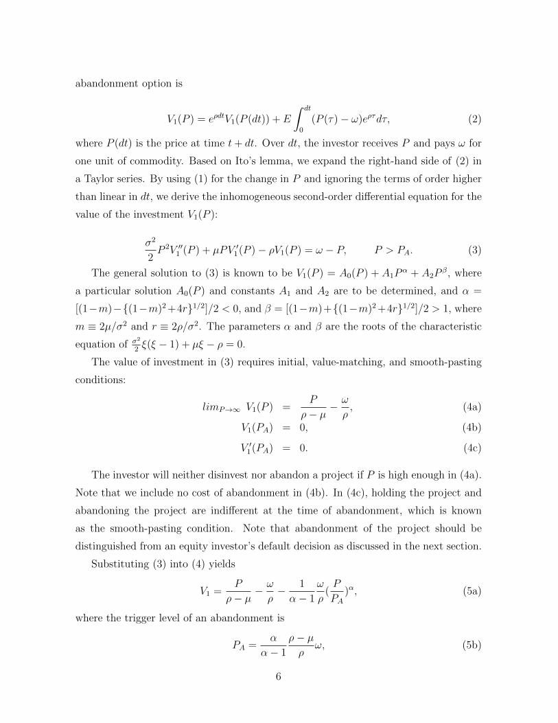
abandonment option is

V1(P ) = eρdtV1(P (dt)) + E

∫ dt

0

(P (τ)− ω)eρτdτ, (2)

where P (dt) is the price at time t+ dt. Over dt, the investor receives P and pays ω for

one unit of commodity. Based on Ito’s lemma, we expand the right-hand side of (2) in

a Taylor series. By using (1) for the change in P and ignoring the terms of order higher

than linear in dt, we derive the inhomogeneous second-order differential equation for the

value of the investment V1(P ):

σ2

2P 2V ′′1 (P ) + µPV ′1(P )− ρV1(P ) = ω − P, P > PA. (3)

The general solution to (3) is known to be V1(P ) = A0(P ) + A1Pα + A2P

β, where

a particular solution A0(P ) and constants A1 and A2 are to be determined, and α =

[(1−m)−(1−m)2 +4r1/2]/2 < 0, and β = [(1−m)+(1−m)2 +4r1/2]/2 > 1, where

m ≡ 2µ/σ2 and r ≡ 2ρ/σ2. The parameters α and β are the roots of the characteristic

equation of σ2

2ξ(ξ − 1) + µξ − ρ = 0.

The value of investment in (3) requires initial, value-matching, and smooth-pasting

conditions:

limP→∞ V1(P ) =P

ρ− µ− ω

ρ, (4a)

V1(PA) = 0, (4b)

V ′1(PA) = 0. (4c)

The investor will neither disinvest nor abandon a project if P is high enough in (4a).

Note that we include no cost of abandonment in (4b). In (4c), holding the project and

abandoning the project are indifferent at the time of abandonment, which is known

as the smooth-pasting condition. Note that abandonment of the project should be

distinguished from an equity investor’s default decision as discussed in the next section.

Substituting (3) into (4) yields

V1 =P

ρ− µ− ω

ρ− 1

α− 1

ω

ρ(P

PA)α, (5a)

where the trigger level of an abandonment is

PA =α

α− 1

ρ− µρ

ω, (5b)

6

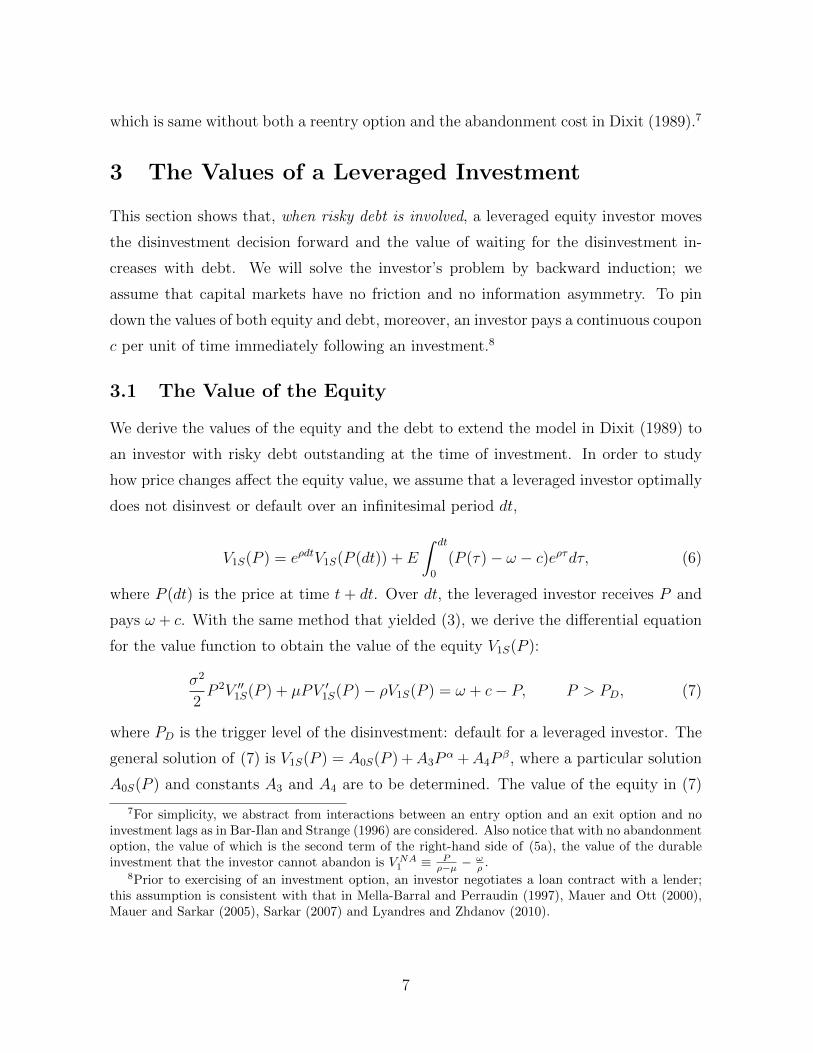
which is same without both a reentry option and the abandonment cost in Dixit (1989).7

3 The Values of a Leveraged Investment

This section shows that, when risky debt is involved, a leveraged equity investor moves

the disinvestment decision forward and the value of waiting for the disinvestment in-

creases with debt. We will solve the investor’s problem by backward induction; we

assume that capital markets have no friction and no information asymmetry. To pin

down the values of both equity and debt, moreover, an investor pays a continuous coupon

c per unit of time immediately following an investment.8

3.1 The Value of the Equity

We derive the values of the equity and the debt to extend the model in Dixit (1989) to

an investor with risky debt outstanding at the time of investment. In order to study

how price changes affect the equity value, we assume that a leveraged investor optimally

does not disinvest or default over an infinitesimal period dt,

V1S(P ) = eρdtV1S(P (dt)) + E

∫ dt

0

(P (τ)− ω − c)eρτdτ, (6)

where P (dt) is the price at time t + dt. Over dt, the leveraged investor receives P and

pays ω + c. With the same method that yielded (3), we derive the differential equation

for the value function to obtain the value of the equity V1S(P ):

σ2

2P 2V ′′1S(P ) + µPV ′1S(P )− ρV1S(P ) = ω + c− P, P > PD, (7)

where PD is the trigger level of the disinvestment: default for a leveraged investor. The

general solution of (7) is V1S(P ) = A0S(P ) +A3Pα +A4P

β, where a particular solution

A0S(P ) and constants A3 and A4 are to be determined. The value of the equity in (7)

7For simplicity, we abstract from interactions between an entry option and an exit option and noinvestment lags as in Bar-Ilan and Strange (1996) are considered. Also notice that with no abandonmentoption, the value of which is the second term of the right-hand side of (5a), the value of the durableinvestment that the investor cannot abandon is V NA1 ≡ P

ρ−µ −ωρ .

8Prior to exercising of an investment option, an investor negotiates a loan contract with a lender;this assumption is consistent with that in Mella-Barral and Perraudin (1997), Mauer and Ott (2000),Mauer and Sarkar (2005), Sarkar (2007) and Lyandres and Zhdanov (2010).

7

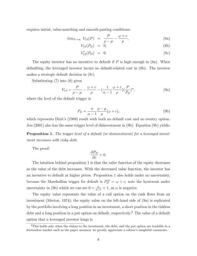
requires initial, value-matching and smooth-pasting conditions:

limP→∞ V1S(P ) =P

ρ− µ− ω + c

ρ, (8a)

V1S(PD) = 0, (8b)

V ′1S(PD) = 0. (8c)

The equity investor has no incentive to default if P is high enough in (8a). When

defaulting, the leveraged investor incurs no default-related cost in (8b). The investor

makes a strategic default decision in (8c).

Substituting (7) into (8) gives

V1S =P

ρ− µ− ω + c

ρ− (

1

α− 1

ω + c

ρ)(P

PD)α, (9a)

where the level of the default trigger is

PD =α

α− 1

ρ− µρ

(ω + c), (9b)

which represents Dixit’s (1989) result with both no default cost and no reentry option.

Jou (2001) also has the same trigger level of disinvestment in (9b). Equation (9b) yields:

Proposition 1. The trigger level of a default (or disinvestment) for a leveraged invest-

ment increases with risky debt.

The proof:∂PD∂c

> 0.

The intuition behind proposition 1 is that the value function of the equity decreases

as the value of the debt increases. With the decreased value function, the investor has

an incentive to default at higher prices. Proposition 1 also holds under no uncertainty,

because the Marshallian trigger for default is PMD = ω + c; note the hysteresis under

uncertainty in (9b) which we can see 0 < αα−1

< 1, as α is negative.

The equity value represents the value of a call option on the cash flows from an

investment (Merton, 1974); the equity value on the left-hand side of (9a) is replicated

by the portfolio involving a long position in an investment, a short position in the riskless

debt and a long position in a put option on default, respectively.9 The value of a default

option that a leveraged investor longs is

9This holds only when the claims to the investment, the debt, and the put option are tradable in africtionless market such as the paper assumes; we greatly appreciate a referee’s insightful comments.

8

Ω(c) ≡ (1

1− αω + c

ρ)(P

PD)α. (10)

Proposition 2. The value of waiting to default (or disinvestment) for a leveraged in-

vestment increases with risky debt.

See appendix A.1 for the derivation.

By taking the financial risk, our investor obtains the positive value of an option of

waiting to default, which increases the value of the equity. The greater leverage exposes

a leveraged investor to higher levels of financial risk, and makes the default option more

valuable.10

An investor nonetheless makes a strategic default decision according to the equity

value, which includes the positive value of waiting in (10). The effect of the reduced

value of the equity dominates the effect of the increased financial risk, even though

higher levels of financial risk caused by an increase in risky debt increase the equity

value. When P > PD, note that ∂V1S(P )∂c

is negative as ∂V1S(P )∂c

= −1ρ− 1

ρ(α−1)( PPD

)α +

( αα−1

ω+cρ

)( PPD

)αP−1D

∂PD∂c

= −1ρ

+ 1ρ( PPD

)α = −1ρ(1 − ( P

PD)α), where the first term is the

effect of the reduced equity value and the second term is the effect of the increased

financial risks.11 Due to a default option, moreover, the marginal value of waiting,∂V1S∂P

= 1ρ−µ(1 − ( P

PD)α−1), decreases as leverage increases;

∂V 21S

∂P∂c= ρ

α(ω+c)( PPD

)α−1 < 0.

Note that when P ≥ PD an increase in risky debt leads to a decrease in the marginal

value of the equity. A leveraged investor has a weaker incentive for waiting to default

because she shares the marginal value of waiting with a debt provider.

In closing this section, note that the value of a default option decreases as the value

of cash flows from a project increases: ∂Ω(c)∂P

< 0. As the value of cash flows from the

project increases, the equity investor becomes less exposed to risk; the leveraged investor

is less likely to default.

10With safe debt, the equity value in (9a) converts to V NA1S ≡ Pρ−µ −

ω+cρ for a leveraged investor

who cannot default on the debt and the value of the debt for a lender who bears no risk is constant atV NA1D ≡ c

ρ over time.11This seems to be strange because a leveraged investor’s marginal value function at P = PD is

irrelevant to financial structure; ∂V1S(PD)∂c =

∂V NA1S

∂c , which equals the marginal value of equity with nodefault option (under no uncertainty) with respect to the coupon. For the investor, however, holdingthe project and defaulting on the loan are indifferent at the trigger.

9

3.2 The Value of the Debt

In order to study how price changes affect the value of debt, we can define the value of

the debt as:

V1D(P ) = eρdtV1D(P (dt)) + E

∫ dt

0

ceρτdτ. (11)

Following the same steps that yielded equation (7) yields

σ2

2P 2V ′′1D(P ) + µPV ′1D(P )− ρV1D(P ) = −c, P > PD (12)

The general solution of (12) is V1D(P ) = A0D(P )+A5Pα+A6P

β, where a particular

solution A0D(P ) and constants A5 and A6 are to be determined. The value of the debt

in (12) requires initial and boundary conditions:

limP→∞ V1D(P ) =c

ρ, (13a)

V1D(PD) = V1(PD). (13b)

If the price is high enough in (13a), the value of risky debt equals the value of

safe debt. When an investor disinvests, the default property is transferred costlessly

to the lender in (13b). Notice that the lender has an abandonment option, but the

abandonment option will be exercised after default, which is determined by the leveraged

investor in (9b).

Substituting (12) into (13) gives the value of the debt as

V1D(P ) =c

ρ+ (

1

α− 1

ω + c

ρ)(P

PD)α − 1

α− 1

ω

ρ(P

PA)α, (14)

where PA < PD in (5b) and (9b), respectively. In equation (14), the lender evaluates

the investor’s incentives and incorporates them in the debt valuation (Harris and Raviv,

1991).

Waiting for information is beneficial to the lender; the value of the debt increases

with the output price. As the output price increases, both the default option and the

abandonment option decrease in value; as the price increases, the equity investor is less

likely to default on the loan and the lender is less likely to abandon the project. While

the lender shorts a default option, the lender longs an abandonment option in (14). The

former default effect dominates the latter abandonment effect. To see this, take the

derivative of (14) with respect to P ,

∂V1D(P )

∂P=Pα−1

ρ− µ(P 1−α

D − P 1−αA ) > 0. (15)

10

In closing this section, note that the value of an investment in (5a) is

V1 = V1S + V1D, (16)

in (9a) and (14), respectively. Equation (16) is independent of the tax rate or bankruptcy

cost, which can be important for firms with debt financing, as shown in Jung and Kim

(2008) and Ko and Yoon (2011). Our approach diverges from that of Mauer and Ott

(2000) and Mauer and Sarkar (2005), but is close to that of Modigliani and Miller (1958)

and Mella-Barral and Perraudin (1997). We contribute to the literature by considering

a lender’s abandonment in equation (16).

4 The Value of the Leveraged Investment Option

This section analyzes the effects of newly issued debt on the timing of an investment.

With risky debt, a leveraged investor moves the investment decision forward and the

value of waiting for the investment decreases.

In order to study how price changes affect the value of an investment opportunity,

we assume that it is optimal not to invest over an infinitesimal period dt.

V0(P ) = e−ρdtV0(P (dt)). (17)

An investor with no assets-in-place holds only an investment option and has no cash

inflow before exercising such an option in (17). Our modeling approach differs from

that of Lyandres and Zhdanov (2010) and Sarkar (2007) because V0 is independent of

assets-in-place with no preexisting debt. As a result, we examine an investment for a

new project with debt outstanding rather than expansion.

Using the same method that yielded (3), we derive the differential equation for an

investment option V0(P )

σ2

2P 2V ′′0 (P ) + µPV ′0(P )− ρV0(P ) = 0, P < PS, (18)

where PS is the trigger level of the leveraged investment.

The general solution for the homogeneous second-order differential equation in (18)

is V0(P ) = A7Pα + A8P

β, where A7 and A8 are constants to be determined.

11

The value of an investment opportunity must satisfy the following boundary condi-

tions12:

limP→0 V0(P ) = 0, (19a)

V0(PS) = V1S(PS)− (k − b), (19b)

V ′0(PS) = V ′1S(PS), (19c)

where

b = V1D(PS) (19d)

in (14). An investor will not exercise an investment option if P is low enough in (19a).

At the time of an investment, the value of an option equals the value of a leveraged

investment in (19b); the equity investor incurs no loss or receives no gain. In addition,

when investing, the investor takes out a new loan. The investor makes an optimal

decision in (19c) and the lender underwrites the loan at fair market value in (19d).

Nonetheless, the pre-determined coupon must be weakly less than a maximum coupon

c, which is determined by ∂V1D(PS :c)∂c

= 0.13

Substituting (18) into (19) gives the value of an investment option,

V0(P ) = (PSρ− µ

− 1

ρ(ω + c+ ρ(k − b))− (

1

α− 1

ω + c

ρ)(PSPD

)α)(P

PS)β

= (PSρ− µ

− ω

ρ− 1

α− 1

ω

ρ(PSPA

)α − k)(P

PS)β, (20a)

where the trigger level of a leveraged investment is

PS =

ββ−1

ρ−µρ

(ω + ρk) + 1α

ββ−1

(PSPA

)αPA

1 + 1β−1

( PSPD

)α−1. (20b)

For the proof of (20b), see appendix A.2.

Proposition 3. A unique PS in (20b) exists where P > PD.

12If an investor maximizes the value of an investment, the value-matching condition in (19b) isV0(P ) = V1(P ) − k, and the smooth-pasting condition in (19c) is V ′0(P ) = V ′1(P ), where P is theinvestment trigger. With no tax advantage, the value maximizer has no incentive to move the investmentdecision even with leverage. For details, see Jou (2001).

13We know that c is determined by ∂V1D(PS :c)∂c = 1

ρ (1− ( PSPD(c) )α) = 0. Furthermore, the second-order

condition is ∂2V1D(P :c)∂c2 = −∂

2Ω(P :c)∂c2 < 0.

12

For the proof, see appendix A.3.1.

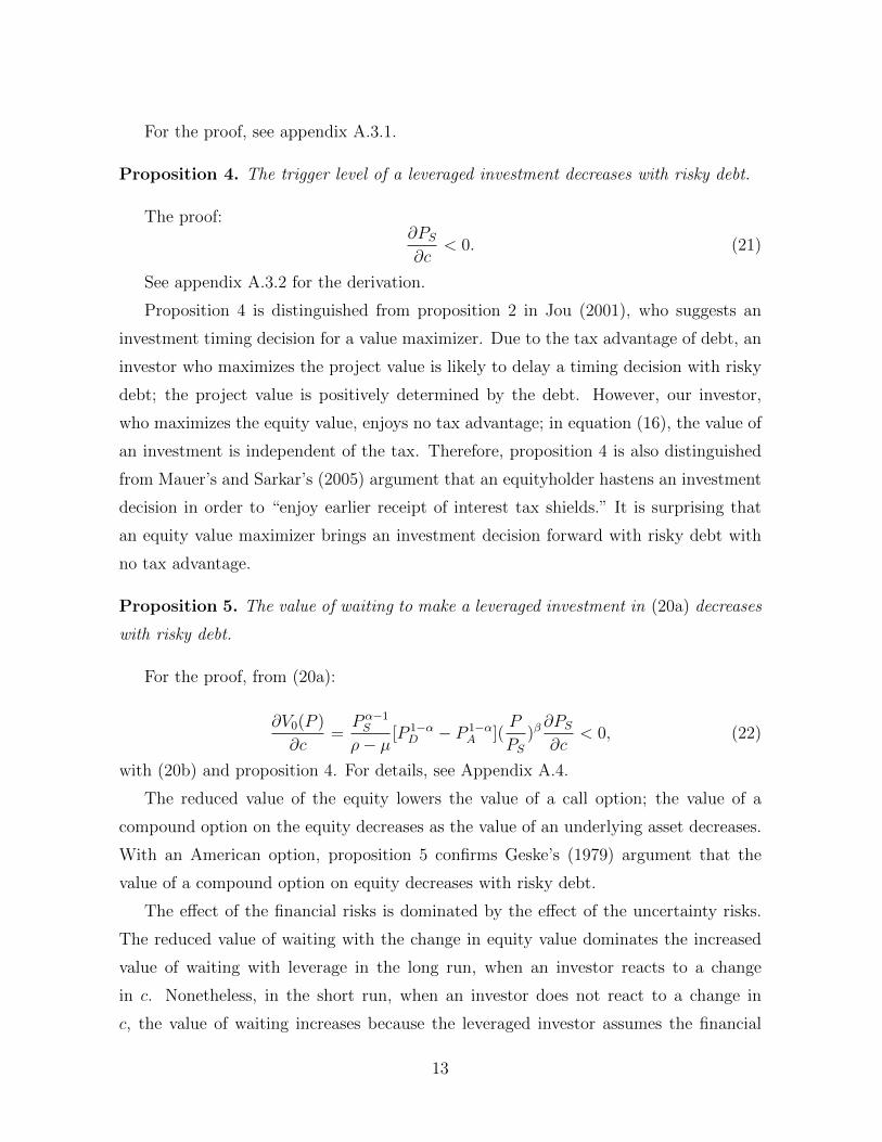
Proposition 4. The trigger level of a leveraged investment decreases with risky debt.

The proof:∂PS∂c

< 0. (21)

See appendix A.3.2 for the derivation.

Proposition 4 is distinguished from proposition 2 in Jou (2001), who suggests an

investment timing decision for a value maximizer. Due to the tax advantage of debt, an

investor who maximizes the project value is likely to delay a timing decision with risky

debt; the project value is positively determined by the debt. However, our investor,

who maximizes the equity value, enjoys no tax advantage; in equation (16), the value of

an investment is independent of the tax. Therefore, proposition 4 is also distinguished

from Mauer’s and Sarkar’s (2005) argument that an equityholder hastens an investment

decision in order to “enjoy earlier receipt of interest tax shields.” It is surprising that

an equity value maximizer brings an investment decision forward with risky debt with

no tax advantage.

Proposition 5. The value of waiting to make a leveraged investment in (20a) decreases

with risky debt.

For the proof, from (20a):

∂V0(P )

∂c=Pα−1S

ρ− µ[P 1−αD − P 1−α

A ](P

PS)β∂PS∂c

< 0, (22)

with (20b) and proposition 4. For details, see Appendix A.4.

The reduced value of the equity lowers the value of a call option; the value of a

compound option on the equity decreases as the value of an underlying asset decreases.

With an American option, proposition 5 confirms Geske’s (1979) argument that the

value of a compound option on equity decreases with risky debt.

The effect of the financial risks is dominated by the effect of the uncertainty risks.

The reduced value of waiting with the change in equity value dominates the increased

value of waiting with leverage in the long run, when an investor reacts to a change

in c. Nonetheless, in the short run, when an investor does not react to a change in

c, the value of waiting increases because the leveraged investor assumes the financial

13

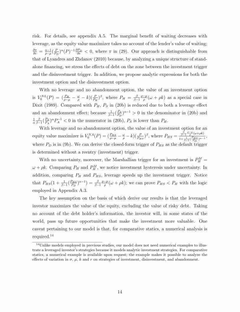
risk. For details, see appendix A.5. The marginal benefit of waiting decreases with

leverage, as the equity value maximizer takes no account of the lender’s value of waiting;∂π∂c

= α−1ρ−µ( P

PD)α(P )−1 ∂PD

∂c< 0, where π in (29). Our approach is distinguishable from

that of Lyandres and Zhdanov (2010) because, by analyzing a unique structure of stand-

alone financing, we stress the effects of debt on the zone between the investment trigger

and the disinvestment trigger. In addition, we propose analytic expressions for both the

investment option and the disinvestment option.

With no leverage and no abandonment option, the value of an investment option

is V NL0 (P ) = ( PH

ρ−µ −ωρ− k)( P

PH)β, where PH = β

β−1ρ−µρ

(ω + ρk) as a special case in

Dixit (1989). Compared with PH , PS in (20b) is reduced due to both a leverage effect

and an abandonment effect; because 1β−1

( PSPD

)α−1 > 0 in the denominator in (20b) and1α

ββ−1

(PSPA

)αP−1A < 0 in the numerator in (20b), PS is lower than PH .

With leverage and no abandonment option, the value of an investment option for an

equity value maximizer is V NA0 (P ) = (PHS

ρ−µ −ωρ− k)( P

PHS)β, where PHS =

ββ−1

ρ−µρ

(ω+ρk)

1+ 1β−1

(PHSPD

)α−1,

where PD is in (9b). We can derive the closed-form trigger of PHS as the default trigger

is determined without a reentry (investment) trigger.

With no uncertainty, moreover, the Marshallian trigger for an investment is PMH =

ω + ρk. Comparing PH and PMH , we notice investment hysteresis under uncertainty. In

addition, comparing PH and PHS, leverage speeds up the investment trigger. Notice

that PHS(1 + 1β−1

(PHSPD

)α−1) = ββ−1

ρ−µρ

(ω + ρk); we can prove PHS < PH with the logic

employed in Appendix A.3.

The key assumption on the basis of which derive our results is that the leveraged

investor maximizes the value of the equity, excluding the value of risky debt. Taking

no account of the debt holder’s information, the investor will, in some states of the

world, pass up future opportunities that make the investment more valuable. One

caveat pertaining to our model is that, for comparative statics, a numerical analysis is

required.14

14Unlike models employed in previous studies, our model does not need numerical examples to illus-trate a leveraged investor’s strategies because it models analytic investment strategies. For comparativestatics, a numerical example is available upon request; the example makes it possible to analyze theeffects of variation in σ, µ, k and r on strategies of investment, disinvestment, and abandonment.

14

5 Conclusion

We have created a model of leveraged investment in an uncertain investment environ-

ment. In particular, we have explored the effects of risky debt on timing decisions for

investment and disinvestment for a leveraged investor; with risky debt, a leveraged eq-

uity investor moves both investment decisions and disinvestment decisions forward. In

addition, risky debt lowers the value of the investment option, while increasing the value

of the disinvestment (or default) option.

Nevertheless, to obtain empirical evidence, it is critical to control for interactions

between existing leverage and the investment decision; unlike in our analysis, previous

studies, such as Mauer and Ott (2000) and Lyandres and Zhdanov (2010), stress the

roles of assets-in-place before an investment is made. In addition, a key assumption

of our model is that a leveraged investor maximizes the value of an equity investment.

Moreover, we rule out a decision to invest on the part of the value maximizer in Jou

(2001). Therefore, referencing general managers of firms, who are likely to consider

the total value of an investment, would be inappropriate for testing our theory. We

suggest seeking empirical evidence from industries in which equity investors with no

assets-in-place play a key role in timing decisions.

15

A Proofs

A.1 Proposition 3

By taking the derivative of equation (10) with respect to c, we have

∂Ω(c)

∂c=

1

1− α1

ρ(P

PD)α − α

1− αω + c

ρ(P

PD)αP−1

D

∂PD∂c

=1

ρ(P

PD)α > 0,

with equation (9b).

A.2 Equation (20b)

PS =

1ρ(ω + ρk)− b+ c

ρ+ ( 1

α−1ω+cρ

)( PSPD

)α

β−1β

1ρ−µ + α

β( 1α−1

ω+cρ

)( PSPD

)α(PS)−1

=

1ρ(ω + ρk) + 1

α−1ωρ(PSPA

)α

β−1β

1ρ−µ + α

β( 1α−1

ω+cρ

)( PSPD

)α(PS)−1

=

ββ−1

ρ−µρ

(ω + ρk) + β 1α−1

1β−1

ρ−µρω(PS

PA)α

1 + α 1α−1

1β−1

ρ−µρ

(ω + c)( PSPD

)αPS−1

=

ββ−1

ρ−µρ

(ω + ρk) + 1α

ββ−1

(PSPA

)αPA

1 + 1β−1

( PSPD

)α−1. (23)

A.3 Propositions 3 and 4

A.3.1 The proofs of proposition 3

From equation (20b), we define f(P ) ≡ P− ββ−1

ρ−µρ

(ω+ρk) and g(P ) ≡ − 1β−1

( PPD

)αPD+1α

ββ−1

( PPA

)αPA = 1β−1

(−P−α+1D + β

αP−α+1A )Pα. By taking the derivative of g(P ), we

obtain g′(P ) > 0, and g′′(P ) < 0 and also we know limP→∞ g(P ) = 0−. By showing

f(P )− g(P ) ≤ 0 at the lower bound P = PD, we can complete the proof. First,

16

f(PD) = PD −β

β − 1

ρ− µρ

(ω + ρk) ≤ g(PD) = − 1

β − 1PD +

β

α

1

β − 1(PDPA

)αPA ⇔

β

β − 1PD −

β

β − 1

ρ− µρ

(ω + ρk) ≤ β

α

1

β − 1(PDPA

)αPA ⇔

α

α− 1(ω + c)− (ω + ρk) ≤ 1

α

ρ

ρ− µ(PDPA

)αPA ⇔

ω

α− 1+

αc

α− 1− ρk ≤ 1

α

ρ

ρ− µ(PDPA

)αPA =ω

α− 1(PDPA

)α. (24)

From equation (19d), we know, second, that the maximum loan amount is weakly

less than the sunk cost.

b = V1D(PD) =c

ρ+ (

1

α− 1

ω + c

ρ)− 1

α− 1

ω

ρ(PDPA

)α ≤ k ⇔

c+1

α− 1(ω + c)− ρk ≤ ω

α− 1(PDPA

)α ⇔

ω

α− 1+

αc

α− 1− ρk ≤ ω

α− 1(PDPA

)α. (25)

According to both equations (24) and (25), we know f(P ) < g(P ) where P > PD.

Note that the maximum coupon cm is determined by ωα−1

+ αcm

α−1−ρk− ω

α−1(PD(cm)

PA)α = 0

A.3.2 The proofs of proposition 4

While ∂f(P )∂c

= 0, ∂g(P )∂c

= −1−αβ−1

PαP−αD∂PD∂c

< 0 with ∂PD∂c

> 0. Along with the proofs of

existence and uniqueness of a solution, ∂PS∂c

< 0.

17

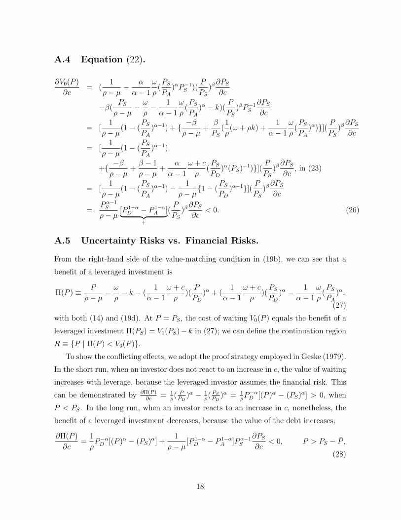
A.4 Equation (22).

∂V0(P )

∂c= (

1

ρ− µ− α

α− 1

ω

ρ(PSPA

)αP−1S )(

P

PS)β∂PS∂c

−β(PSρ− µ

− ω

ρ− 1

α− 1

ω

ρ(PSPA

)α − k)(P

PS)βP−1

S

∂PS∂c

= [1

ρ− µ(1− (

PSPA

)α−1) + −βρ− µ

+β

PS(1

ρ(ω + ρk) +

1

α− 1

ω

ρ(PSPA

)α)]( PPS

)β∂PS∂c

= [1

ρ− µ(1− (

PSPA

)α−1)

+ −βρ− µ

+β − 1

ρ− µ+

α

α− 1

ω + c

ρ(PSPD

)α(PS)−1)]( PPS

)β∂PS∂c

, in (23)

= [1

ρ− µ(1− (

PSPA

)α−1)− 1

ρ− µ1− (

PSPD

)α−1]( PPS

)β∂PS∂c

=Pα−1S

ρ− µ[P 1−αD − P 1−α

A ]︸ ︷︷ ︸+

(P

PS)β∂PS∂c

< 0. (26)

A.5 Uncertainty Risks vs. Financial Risks.

From the right-hand side of the value-matching condition in (19b), we can see that a

benefit of a leveraged investment is

Π(P ) ≡ P

ρ− µ− ω

ρ− k − (

1

α− 1

ω + c

ρ)(P

PD)α + (

1

α− 1

ω + c

ρ)(PSPD

)α − 1

α− 1

ω

ρ(PSPA

)α,

(27)

with both (14) and (19d). At P = PS, the cost of waiting V0(P ) equals the benefit of a

leveraged investment Π(PS) = V1(PS)− k in (27); we can define the continuation region

R ≡ P | Π(P ) < V0(P ).To show the conflicting effects, we adopt the proof strategy employed in Geske (1979).

In the short run, when an investor does not react to an increase in c, the value of waiting

increases with leverage, because the leveraged investor assumes the financial risk. This

can be demonstrated by ∂Π(P )∂c

= 1ρ( PPD

)α − 1ρ( PSPD

)α = 1ρP−αD [(P )α − (PS)α] > 0, when

P < PS. In the long run, when an investor reacts to an increase in c, nonetheless, the

benefit of a leveraged investment decreases, because the value of the debt increases;

∂Π(P )

∂c=

1

ρP−αD [(P )α − (PS)α] +

1

ρ− µ[P 1−αD − P 1−α

A ]Pα−1S

∂PS∂c

< 0, P > PS − P ,(28)

18

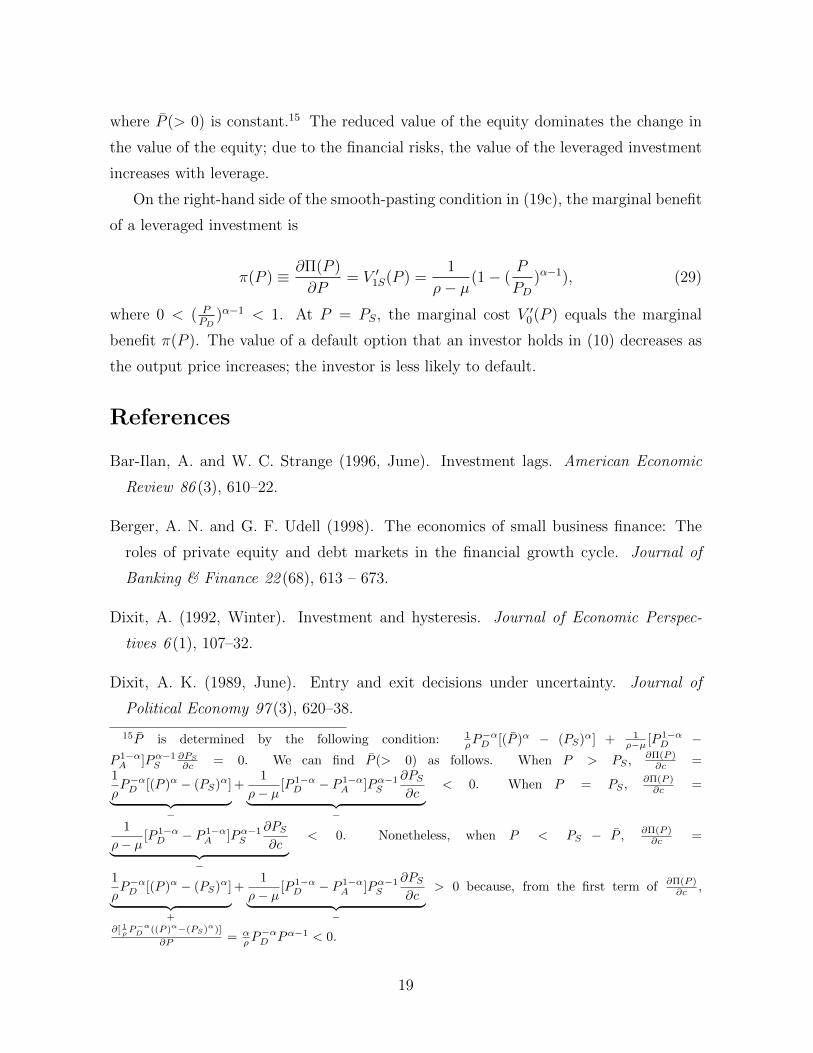
where P (> 0) is constant.15 The reduced value of the equity dominates the change in

the value of the equity; due to the financial risks, the value of the leveraged investment

increases with leverage.

On the right-hand side of the smooth-pasting condition in (19c), the marginal benefit

of a leveraged investment is

π(P ) ≡ ∂Π(P )

∂P= V ′1S(P ) =

1

ρ− µ(1− (

P

PD)α−1), (29)

where 0 < ( PPD

)α−1 < 1. At P = PS, the marginal cost V ′0(P ) equals the marginal

benefit π(P ). The value of a default option that an investor holds in (10) decreases as

the output price increases; the investor is less likely to default.

References

Bar-Ilan, A. and W. C. Strange (1996, June). Investment lags. American Economic

Review 86 (3), 610–22.

Berger, A. N. and G. F. Udell (1998). The economics of small business finance: The

roles of private equity and debt markets in the financial growth cycle. Journal of

Banking & Finance 22 (68), 613 – 673.

Dixit, A. (1992, Winter). Investment and hysteresis. Journal of Economic Perspec-

tives 6 (1), 107–32.

Dixit, A. K. (1989, June). Entry and exit decisions under uncertainty. Journal of

Political Economy 97 (3), 620–38.

15P is determined by the following condition: 1ρP−αD [(P )α − (PS)α] + 1

ρ−µ [P 1−αD −

P 1−αA ]Pα−1

S∂PS∂c = 0. We can find P (> 0) as follows. When P > PS , ∂Π(P )

∂c =1

ρP−αD [(P )α − (PS)α]︸ ︷︷ ︸

−

+1

ρ− µ[P 1−αD − P 1−α

A ]Pα−1S

∂PS∂c︸ ︷︷ ︸

−

< 0. When P = PS , ∂Π(P )∂c =

1

ρ− µ[P 1−αD − P 1−α

A ]Pα−1S

∂PS∂c︸ ︷︷ ︸

−

< 0. Nonetheless, when P < PS − P , ∂Π(P )∂c =

1

ρP−αD [(P )α − (PS)α]︸ ︷︷ ︸

+

+1

ρ− µ[P 1−αD − P 1−α

A ]Pα−1S

∂PS∂c︸ ︷︷ ︸

−

> 0 because, from the first term of ∂Π(P )∂c ,

∂[ 1ρP−αD ((P )α−(PS)α)]

∂P = αρP−αD Pα−1 < 0.

19

Esty, B. C. (2004). Why study large projects? an introduction to research on project

finance. European Financial Management 10 (2), 213–224.

Geske, R. (1979, March). The valuation of compound options. Journal of Financial

Economics 7 (1), 63–81.

Harris, M. and A. Raviv (1991). The theory of capital structure. The Journal of

Finance 46 (1), pp. 297–355.

Jensen, M. C. and W. H. Meckling (1976, October). Theory of the firm: Managerial

behavior, agency costs and ownership structure. Journal of Financial Economics 3 (4),

305–360.

Jou, J.-B. (2001). Entry, financing, and bankruptcy decisions: The limited liability

effect. The Quarterly Review of Economics and Finance 41 (1), 69–88.

Jung, K. and B. Kim (2008). Corporate cash holdings and tax-induced debt financing.

Asia-Pacific Journal of Financial Studies 37, 983–1023.

Ko, J. K. and S.-S. Yoon (2011). Tax benefits of debt and debt financing in korea.

Asia-Pacific Journal of Financial Studies 40, 824–855.

Lyandres, E. and A. Zhdanov (2010). Accelerated investment effect of risky debt. Journal

of Banking & Finance 34 (11), 2587 – 2599.

Mauer, D. C. and S. Ott (2000). Agency costs, underinvestment, and optimal capital

structure: The effect of growth options to expand. In M. Brennan and L. Trigeorgis

(Eds.), Project Flexibility, Agency, and Competition. Oxford University Press, pp.

151–180. Oxford University Press.

Mauer, D. C. and S. Sarkar (2005, June). Real options, agency conflicts, and optimal

capital structure. Journal of Banking & Finance 29 (6), 1405–1428.

Mella-Barral, P. and W. Perraudin (1997, June). Strategic debt service. Journal of

Finance 52 (2), 531–56.

Merton, R. C. (1974, May). On the pricing of corporate debt: The risk structure of

interest rates. Journal of Finance 29 (2), 449–70.

20

Modigliani, F. and M. H. Miller (1958). The cost of capital, corporation finance and the

theory of investment. The American Economic Review 48 (3), pp. 261–297.

Myers, S. C. (1977). Determinants of corporate borrowing. Journal of Financial Eco-

nomics 5 (2), 147 – 175.

Sarkar, S. (2007). Expansion financing and capital structure. SSRN eLibrary .

Yagi, K., R. Takashima, H. Takamori, and K. Sawaki (2008, August). Timing of con-

vertible debt financing and investment. CARF F-Series CARF-F-131, Center for

Advanced Research in Finance, Faculty of Economics, The University of Tokyo.

21