the early socioeconomic effects of teenage … early socioeconomic effects of teenage childbearing:...
TRANSCRIPT

Demographic Research a free, expedited, online journal of peer-reviewed research and commentary in the population sciences published by the Max Planck Institute for Demographic Research Konrad-Zuse Str. 1, D-18057 Rostock · GERMANY www.demographic-research.org
DEMOGRAPHIC RESEARCH VOLUME 23, ARTICLE 25, PAGES 697-736 PUBLISHED 05 OCTOBER 2010 http://www.demographic-research.org/Volumes/Vol23/25/ DOI: 10.4054/DemRes.2010.23.25 Research Article
The early socioeconomic effects of teenage childbearing: A propensity score matching approach
Dohoon Lee
©2010 Dohoon Lee. This open-access work is published under the terms of the Creative Commons Attribution NonCommercial License 2.0 Germany, which permits use, reproduction & distribution in any medium for non-commercial purposes, provided the original author(s) and source are given credit. See http:// creativecommons.org/licenses/by-nc/2.0/de/

Table of Contents
1 Introduction 698 2 Prior research on the socioeconomic effects of teenage childbearing 699 2.1 Causal vs. selection arguments 699 2.2 Previous empirical strategies 700 3 A counterfactual approach: Propensity score matching with
Rosenbaum bounds 702
3.1 A propensity score matching framework 702 3.2 A sensitivity analysis: Use of Rosenbaum bounds 704 4 Data and measures 705 4.1 Data 705 4.2 Measures 707 4.2.1 Dependent variables 707 4.2.2 Explanatory variables 707 5 Results 709 5.1 Preliminary results 709 5.2 Matching results 714 5.3 Results from the sensitivity analysis 718 5.4 Racial/ethnic differences 721 6 Discussion and conclusion 723 7 Acknowledgements 724 References 725 Appendix A: The Rosenbaum bounds method 730 Appendix B: Covariate balance check 732 Appendix C: Teenage childbearing defined as giving birth before
age 18 734

Demographic Research: Volume 23, Article 25 Research Article
http://www.demographic-research.org 697
The early socioeconomic effects of teenage childbearing: A propensity score matching approach
Dohoon Lee1
Abstract
A large body of literature has documented a negative correlation between teenage childbearing and teen mothers’ socioeconomic outcomes, yet researchers continue to disagree as to whether the association represents a true causal effect. This article extends the extant literature by employing propensity score matching with a sensitivity analysis using Rosenbaum bounds. The analysis of recent cohort data from the National Longitudinal Study of Adolescent Health shows that (1) teenage childbearing has modest but significant negative effects on early socioeconomic outcomes and (2) unobserved covariates would have to be more powerful than known covariates to nullify the propensity score matching estimates. The author concludes by suggesting that more research should be done to address unobserved heterogeneity and the long-term effects of teenage childbearing for this young cohort.
1 Department of Sociology, New York University, 295 Lafayette St., 4th Floor, New York, NY 10012, USA. E-mail:[email protected].

Lee: The early socioeconomic effects of teenage childbearing: A propensity score matching approach
698 http://www.demographic-research.org
1. Introduction
The longstanding literature on teen motherhood has documented its detrimental life cycle consequences. Teen mothers tend to have worse socioeconomic outcomes than other women who delay childbearing (An, Haveman, and Wolfe 1993; Hofferth and Hayes 1987). Despite this evidence, it is still unclear whether these negative outcomes among teen mothers result from the incidence of childbearing per se or from the socioeconomic disadvantages these women faced before they became teen mothers. While human capital theory holds that teenage childbearing has a real causal effect on socioeconomic outcomes because it directly interferes with adolescents’ investment in human capital (Becker 1993), the selection view contends that teenage childbearing is associated with negative outcomes because it occurs mostly among disadvantaged female adolescents (Geronimus, Korenman, and Hillemeier 1994). Indeed, the concern about selection bias points out that isolating the effect of teen motherhood creates a considerable methodological challenge (Winship and Mare 1992; Winship and Morgan 1999): If both observed and unobserved preexisting characteristics of teen mothers account for the relationship between teenage childbearing and its socioeconomic consequences, assertions of causality become questionable.
A large body of research has addressed the selection bias problem by finding better comparison groups for women who give birth in their teens (Cherlin 2001; Hoffman 1998; Korenman, Kaestner, and Joyce 2001; Wu and Wolfe 2001). For example, within-family fixed-effects models compare teen mothers with their sisters who gave birth after their teenage years to control for unobserved family-level heterogeneity (Geronimus and Korenman 1992). Quasi-natural experimental approaches approximate randomization procedures by treating twin births or miscarriages as comparison cases (Grogger and Bronars 1993; Hotz, McElroy, and Sanders 1997). Finally, instrumental variables methods utilize variables that capture the exogenous component of teenage childbearing to mitigate the selection bias problem (Klepinger, Lundberg, and Plotnick 1999). Despite their intuitive appeal, all of these models have their own drawbacks. It is not uncommon to find that they are grounded on somewhat strong assumptions and/or unrepresentative samples, with mixed results at best. Thus, evaluating the “true” effects of teenage childbearing remains an elusive goal.
In this article, I extend the previous literature in three distinct ways. First, I use a propensity score matching approach to identify the early socioeconomic effects of teenage childbearing. Following the counterfactual framework (Rosenbaum and Rubin 1983; Rubin 1977), this approach matches teen mothers (“treatment” group) to those who are not teen mothers but similar in all other preexisting observed characteristics (“control” group), based on a propensity to give birth as teens. Then it compares various socioeconomic outcomes between these two groups using semi-parametric estimators.
Demographic Research: Volume 23, Article 25
http://www.demographic-research.org 699
Second, this article addresses selection bias due to both observed and unobserved covariates. Past studies employing the matching approach have focused mainly on selection bias due to observed covariates (Chevalier and Viitanen 2003; Levine and Painter 2003). Using the Rosenbaum bounds method (Rosenbaum 2002), I evaluate the extent to which selection bias on unobserved covariates would nullify propensity score matching estimates of the effects of teenage childbearing.
Third, I use data from the National Longitudinal Study of Adolescent Health (Add Health), which covers the latest cohort of adolescents who transition into young adulthood. This article clearly recognizes that any estimates of the effects of teenage childbearing should be put in context: the U.S. teen birth rate has steadily declined since 1991, when it was at its peak (Martin et al. 2006);2 the economic returns to education have increased (Morris and Western 1999); a new welfare policy - Personal Responsibility and Work Opportunity Act (PRWORA) - replaced Aid to Families with Dependent Children (AFDC) with Temporary Assistance for Needy Families (TANF); and the influx of immigrants, especially Hispanics, has continued to grow. Add Health allows reflection upon these recent changes and its large sample size facilitates assessing racial/ethnic differences in the socioeconomic consequences of teenage childbearing. Taken together, the counterfactual approach using the Add Health data is expected to provide useful insight into estimating the early socioeconomic effects of teen motherhood.
2. Prior research on the socioeconomic effects of teenage childbearing
2.1 Causal vs. selection arguments
Human capital theory argues that teenage childbearing may have deleterious consequences (Becker 1993). According to this theory, the incidence of early childbearing tends to raise the opportunity costs of accumulation in human capital. Being a teen mother may hinder human capital investment because it is during adolescence that one’s education is attained. Given the high secondary school dropout rates of teen mothers, they are less likely to attain a college degree, which is more valued in labor markets. Teenage motherhood also may keep young women from participating in the labor force due to the incompatibility between employment and child rearing. Since teenagers are still at an early developmental stage of life, being a
2 Nonetheless, the teen birth rate in the U.S. has been the highest among the developed countries (Ventura et al. 2004).
Lee: The early socioeconomic effects of teenage childbearing: A propensity score matching approach
700 http://www.demographic-research.org
mother as a teen makes it more difficult to take the appropriate economic, social, and psychological responsibilities. As a result, teen mothers tend to be more dependent on welfare and trapped in poverty (Furstenberg 1991).
In opposition to this conventional view, the selection view maintains that teenage childbearing does not necessarily cause negative consequences for young mothers (Geronimus 1991). Because the majority of teen mothers come from impoverished families and neighborhoods, simply postponing childbearing may not be sufficient for disadvantaged young women to escape poverty. Moreover, faced with poor conditions and bleak prospects, they may have an incentive for early childbearing as an adaptive strategy. Such behavior can be regarded as a culturally rational response to poverty because childbearing could derive socioeconomic support from extended families and neighborhoods (Geronimus, Korenman, and Hillemeier 1994). Since the adverse consequences of teenage childbearing may be an artifact of the preexisting socioeconomic disadvantages of teen mothers, this view underscores substantive knowledge about the ways in which teen mothers might systematically differ from other young women in order to assess the causal effects of teenage childbearing.
2.2 Previous empirical strategies
These two contrasting views invoke the fundamental problem of causal inference about the effects of teenage childbearing: One cannot observe the outcomes of interest simultaneously for a teenager when she is a teen mother (a treated subject) and when she is not (a control subject) (Holland 1986). In an experimental setup, this problem may be solved by randomization through which the treatment group is identical to the control group in all characteristics other than the treatment assignment. Any remaining differences in the outcomes between the two groups, then, are attributable to the causal effects of the treatment. In most social scientific studies, however, random assignment is not feasible. Teenage childbearing occurs nonrandomly as it is concentrated among the disadvantaged subpopulation. This selection bias problem points out that one should estimate the causal effect of teenage childbearing for young women who experienced it (average treatment effect for the treated) rather than for young women as a whole (average treatment effect) (Dehejia and Wahba 2002; Harding 2003). Therefore, it is crucial to identify a reliable comparison group that does not experience teen motherhood but is similar to teen mothers in preexisting characteristics. A variety of innovative approaches have sought to account for both observed and unobserved differences between teen mothers and other young women (see Hoffman (1998) for a review). They include within-family fixed-effect models, instrumental variables methods, and quasi-natural experimental approaches.

Demographic Research: Volume 23, Article 25
http://www.demographic-research.org 701
Within-family fixed-effect models compare sisters whose childbearing was timed at different ages. Since sisters share the same family and neighborhood characteristics, comparing sisters is expected to eliminate unmeasured environmental factors. Analyzing data from the National Longitudinal Survey of Young Women, Geronimus and Korenman (1992, 1993) show that cross-sectional studies overstate the correlation between teenage childbearing and its negative outcomes, and the effects of early motherhood are minimal in most cases. In contrast, Hoffman, Foster, and Furstenberg (1993a, 1993b) use data from the Panel Study of Income Dynamics and find that previous estimates exaggerate the negative effects of teenage childbearing, but these effects remain sizable. These conflicting findings bear several substantive concerns about the sister comparison. Within-family fixed-effects models are based on somewhat small samples of sisters that come from relatively large families, such that external validity is difficult to adjudicate. Moreover, these models are not very powerful in capturing time-varying individual differences between teen mothers and their sisters. If teen mothers have a lower level of achievement than their sisters, a failure to control for this attribute will make the negative effects of teenage childbearing biased upward. On the other hand, the assumption of shared (i.e., fixed) family background factors is violated if parents divert resources away from the non-childbearing sister to the sister who has a birth, biasing the negative effects downward.
Instrumental variables methods are designed to take the endogeneity of teenage childbearing into account, with attention paid to finding variables that are correlated with teenage childbearing but otherwise unrelated to its socioeconomic outcomes. For instance, age at menarche and various measures regarding abortion have been utilized as instrumental variables. Findings are mixed, with some studies showing no effects of teenage childbearing (Olsen and Farkas 1989; Ribar 1994) and other studies reporting negative effects (Klepinger, Lundberg, and Plotnick 1999). Although these instrumental variables are validated in a statistical sense, the assumption that they have no relation to young women’s outcomes is difficult to test. Furthermore, the instrumental variables methods are likely to estimate the local average treatment effect (Angrist and Krueger 2001; Imbens and Angrist 1994) - i.e., an estimate for only a subset of female teenagers who changed their childbearing behavior due to the early initiation of menarche or the availability of state abortion facilities.
Quasi-natural experimental approaches attempt to identify better comparison groups for teen mothers, such as teen mothers who had twin births or pregnant adolescents who had miscarriages. These comparison groups may not differ from teen mothers in characteristics, because twin births and miscarriages arguably occur randomly. Twin studies show that teenage childbearing has modest but adverse effects on women’s subsequent outcomes for blacks and to a lesser degree, for whites (Grogger and Bronars 1993), while miscarriage studies find that most of the negative effects of

Lee: The early socioeconomic effects of teenage childbearing: A propensity score matching approach
702 http://www.demographic-research.org
teenage childbearing are short-lived and its effects become positive when teen mothers reach their mid- and late 20s (Hotz, McElroy, and Sanders 1997, 2005). However, the findings from both studies need to be cautiously interpreted because twin births and miscarriages are rare events. Also, teen mothers with twins might benefit from economies of scale compared with teen mothers with one child, resulting in an underestimation of the effects of teenage childbearing (Hoffman 1998). Similarly, miscarriage studies would produce biased estimates to the extent that the occurrence of miscarriages is underreported, or miscarriages are correlated with unobserved community-level factors (Fletcher and Wolfe 2009).
3. A counterfactual approach: Propensity score matching with Rosenbaum bounds
3.1 A propensity score matching framework
In the spirit of the counterfactual analysis with observational data, this study takes a propensity score matching approach (Morgan and Winship 2007). One could imagine that two young women are matched on the same preexisting observed characteristics, one of whom is a teen mother and the other is not. Each unit of observation could be stratified into subgroups according to a specific value of covariates. However, as more covariates are needed to ensure the determinants of teenage childbearing, there should be an increasing number of cells that contain no comparison unit. Rosenbaum and Rubin (1983) suggest that propensity score matching greatly reduces the high dimensionality of the observed covariates by constructing a propensity score, the probability of receiving treatment assignment. If the true propensity score is known, a pair of the treatment and the matched control groups would, in expectation, be balanced on both observed and unobserved preexisting characteristics. Since this is improbable in practice, the predicted probabilities of receiving treatment assignment calculated from a logit (or probit) model serve as the estimated propensity scores to match the treatment and control groups based on preexisting observed covariates.
The analysis takes this approach as follows. First, it estimates a logit model to calculate the predicted probabilities of teen motherhood, which are used as the propensity scores. In this model, all observed covariates are measured prior to occurrence of teenage childbearing. Drawing on previous literature, I carefully select sociodemographic-, individual-, school-, and neighborhood-level determinants of teenage childbearing status (see section 4, Data and measures).
Second, using the propensity scores, it generates a sample consisting of teen mothers and their matched cases. Among young women who are not teen mothers, the

Demographic Research: Volume 23, Article 25
matched cases include only those who are close enough to teen mothers in terms of the propensity scores.3 Among a variety of matching algorithms, I consider single-nearest-neighbor caliper matching with replacement (Morgan and Harding 2006).4 The caliper size set in the analysis is .01, which restricts matches to have differences in the propensity scores within one percentage point.
Third, it examines whether teen mothers and their matched counterparts are balanced on observed covariates. I test whether the logit model from which the propensity scores are calculated achieves a significant reduction in absolute bias - the standardized percentage mean difference in each covariate between the treatment and control groups.5 If this propensity score estimation model is well specified, there should be little difference in preexisting observed covariates between these two groups.
Finally, it assesses differences in the socioeconomic outcomes between teen mothers and their matched counterparts. To minimize reverse causality, all outcome variables are measured after teen birth. For the purpose of comparison, I also present standard regression estimates of the effects of teenage childbearing.
In fact, the propensity matching approach would produce similar estimates to those from regression-based models if these models met all of the prerequisite assumptions and had well-supported data. However, when these conditions cannot be satisfied, the propensity score matching method has clear advantages over parametric approaches. First, it avoids serious mismatches between those who gave birth as teens and those who were least likely to do so, by matching only similar cases. Standard regression methods are likely to retain these mismatches, producing unrealistic average treatment effect. Second, the propensity score matching method is semi-parametric with no assumption of functional forms for the relationship between the treatment variable and the outcomes of interest. Standard regression methods should assume a specific functional form that results in extrapolation and smoothing, which are prone to biases due to serious mismatches.6 Third, the propensity score matching estimators are known to be more efficient and free from collinearity because only the estimated propensity scores are required.
http://www.demographic-research.org 703
3 One might think that the control group should contain only young women who gave birth after their teenage years. However, this may cause the simultaneity problem, by which outcomes affect the control group’s childbearing status. 4 Switching the matching algorithms does not alter the findings reported here (the results are available upon request from the author). 5 The absolute bias is calculated as a percentage of the mean difference divided by the average standard deviation for the two groups: .2/)22()(100Bias CsTsCxTx +−=
6 On the other hand, the propensity score matching method should make an assumption about the functional form of the model predicting teenage childbearing status, which standard regression methods do not need to make. However, as Harding (2003) suggests, this assumption can be verified by assessing whether the matching procedure achieves covariate balance.

Lee: The early socioeconomic effects of teenage childbearing: A propensity score matching approach
704 http://www.demographic-research.org
It should be noted that in the propensity score matching procedure, a certain portion of teen mothers still may not have their counterfactuals in the matched sample if their propensity scores are too high to find their matches in the comparison group. This common support problem implies that if so, one can only estimate the causal effects of teenage childbearing for the subset of the treated group (Heckman, Ichimura, and Todd 1998). I address this issue by evaluating how well the treated group overlaps with the control group by way of the propensity score matching procedure. In addition, like conventional regression analysis, the propensity score matching method assumes no selection bias on unobserved covariates, which posits that conditional on preexisting observed covariates, teenage childbearing is independent of the outcome of interest (Rubin 1977). However, the matching framework used here can evaluate this ignorable treatment assignment assumption by incorporating a sensitivity analysis that examines how large the selection bias problem would need to be to completely wipe out propensity score matching estimates of the effect of teenage childbearing. I demonstrate below how the sensitivity analysis can be employed in the matching framework.
3.2 A sensitivity analysis: Use of Rosenbaum bounds
The counterfactual analysis of teenage childbearing may be sensitive to “hidden bias” due to preexisting unobserved characteristics that influence both teenage childbearing status and its outcomes, even if this approach achieves a balance between teen mothers and their matched counterparts in terms of preexisting observed characteristics. Previous studies using propensity score matching do not fully account for this possibility (Chevalier and Viitanen 2003; Levine and Painter 2003). For example, a researcher might not know how families decide where to live. If this decision-making process matters both for the incidence of teenage childbearing and for its outcomes, the true effects of early motherhood will not be estimated correctly. The sensitivity analysis developed by Rosenbaum (2002) addresses the strength of such an unobserved variable to evaluate the causal effects estimated from propensity score matching (see Appendix A for a formal notation).
Suppose that a confounding unobserved covariate, U, exists that affects the odds of being assigned to the treatment, T, conditional on observed covariates, X. If U has nothing to do with T, then the assignment process is regarded as random. But as the influence of U on T becomes stronger, the confidence interval on the estimated effect of T becomes wider, and the significance level of the test of the null hypothesis of no effect of T on the outcome increases (i.e., the p-value goes up). In this scenario, one gauges the end points on the bounds for the significance level of the test of the null hypothesis for each assumed level of association between U and T. This enables one to

Demographic Research: Volume 23, Article 25
http://www.demographic-research.org 705
find the case where the effect of U on the outcome is so strong that knowledge about U would almost perfectly predict the level of the outcome, whether or not a unit of observation received treatment assignment. In this regard, while not calibrating the exact size of the true effect of teenage childbearing in the presence of unobserved heterogeneity, the Rosenbaum bounds method provides a basis for assessing the selection bias problem by making explicit the extent to which the ignorable treatment assignment assumption underlying the propensity score matching is vulnerable (DiPrete and Gangl 2004).
A key feature of this method is to allow a researcher to benchmark the strength of unobserved confounding variable against that of observed variables, because many of the determinants of teenage childbearing have been identified in the literature. For instance, family structure is known to have a powerful effect on early motherhood and its outcomes (Wu and Martinson 1993). By comparing the magnitude of hidden bias with that of the known observed covariates, we can examine the strength of selection bias due to unobserved covariate required to alter the causal inference about the effects of teenage childbearing.
4. Data and measures
4.1 Data
This study uses data from the National Longitudinal Study of Adolescent Health (Add Health). Add Health is a nationally representative, multistage, stratified, school-based, longitudinal study of adolescents in grade 7 to 12 in 1994-1995 (Harris et al. 2009). An In-school questionnaire was administered to more than 90,000 adolescents who attended the sampled schools on a particular day during the period of September 1994 to April 1995. Based on the school rosters, a random sample of about 200 students from each high school and feeder school pair was collected between April and December 1995, yielding the core In-home sample of about 12,000 adolescents. Adding special over-samples that included racial/ethnic minorities, physically disabled adolescents, and a genetic sample, the Wave I data produced a total sample size of 20,745 adolescents, 10,480 of whom are female. Their parents also were interviewed in Wave I. In 2001 and 2002, approximately 15,200 Wave I respondents, 8,030 of whom are female, were re-interviewed in Wave III to investigate the influences that experiences in adolescence have on young adulthood.7
7 The age range at Wave III is from 18 to 27 with the average age of 22. That the data consist of young adults implies that despite the strong correlations between early and late socioeconomic behaviors, the results reported here refer to the early socioeconomic effects of teen motherhood.

Lee: The early socioeconomic effects of teenage childbearing: A propensity score matching approach
706 http://www.demographic-research.org
It appears that Add Health may not be representative of all adolescents because it uses a school-based design and misses high school dropouts in the In-school survey. As Udry and Chantala (2003) demonstrate, however, annual dropout rates are very low at the national level; the In-home sample was selected from the school rosters, which were collected approximately a year before the Wave I In-home interviews, so the only dropouts missed are those who dropped out of school two years prior to the Wave I In-home interviews. Indeed, a preliminary analysis (not shown) indicates that sociodemographic characteristics differ little by age. While missing dropouts remains a concern, it does not seem to alter the results reported here.
Because of its strong emphasis on social contexts and its broad definition of health-related behaviors, Add Health provides valuable information well suited for this study. First, the Wave III sample contains detailed data on fertility, educational attainment, labor market performance, and public assistance receipt. Second, the Wave I sample provides a rich set of variables that are measured prior to the incidence of teenage childbearing.8 It also contains variables that are previously unmeasured but considered key factors of teenage childbearing and various socioeconomic outcomes. For example, recent evidence shows that personality traits such as locus of control and self-esteem play an important role in teenage childbearing and subsequent outcomes (Heckman, Stixrud, and Urzua 2006).
Finally, Add Health allows an up-to-date assessment of the effects of teenage childbearing. Timeliness is an important issue given significant contextual changes during the 1990s (Hoffman 1998). The 1990s witnessed growing economic return to education, changes in welfare policy, and the increase of Hispanics in the U.S. adolescent population, all of which could have influences on adolescents’ fertility behavior. This study does not address the direct impacts of these social changes on the association between teenage childbearing and its outcomes, but does discuss the implications of the recent contextual changes and analyzes race/ethnicity-specific samples alongside the whole sample.
The analytic sample consists of 6,825 adolescent females who were interviewed at Waves I and III and who had observations on teenage childbearing status, the dependent and explanatory variables of interest, and sampling weights. A preliminary analysis suggests that there is little difference between the analytic sample and the sample before listwise deletion. To account for the sampling design effects in Add Health, all analyses adjust standard errors for school-level clustering.
8 There were older teenagers at risk for giving birth prior to Wave I. Since all covariates come from Wave I, this might cause reverse causality between teenage childbearing and some of the covariates. I reestimated all models presented here with and without those who became mothers by Wave I. In addition, all of these models were reanalyzed by limiting the analytic sample to adolescents who did not give birth and were younger than age 16 at Wave I. The results in both cases (available upon request from the author) do not alter the findings shown here.
Demographic Research: Volume 23, Article 25
http://www.demographic-research.org 707
4.2 Measures
4.2.1 Dependent variables
Educational Attainment: Two measures of educational attainment come from the Wave III data: dropping out of high school and attending or graduating from some college (2 year or more). I treat GED recipients as high school graduates. Since there is little consensus on whether GED recipients are considered high school dropouts or graduates (Cameron and Heckman 1993; Cao, Stromsdorfer, and Weeks 1996; Upchurch and McCarthy 1990), I reestimated the analyses to treat GED recipients as high school dropouts. Also, I used attending or graduating from college (4 year or more) instead of some college for another robustness check. The results (not shown) are similar to those presented below.
Labor Market Outcomes: Employment status, work-related activities, full-time/part-time status, and weekly wages are obtained from the Wave III data. Work-related activities include on-the-job-training as well as employment status. Weekly wages below the 3rd percentile in the wage distribution are set equal to the 3rd percentile, and weekly wages above the 97th percentile are set equal to the 97th percentile. Log-transformed weekly wages are used for analyses. Since there are respondents who still were enrolled in post-secondary schools at Wave III, I restrict the samples to respondents not in schools. I further restrict the samples to respondents who were employed at Wave III for full-time/part-time status and those who worked full-time for weekly wages.
Public Assistance Receipt: This variable identifies whether respondents were on welfare at Wave III and ever on welfare. A respondent is identified as welfare-dependent if she received AFDC (or TANF), public assistance, welfare payments, or food stamps.
4.2.2 Explanatory variables
Teenage Childbearing: Teenage childbearing status is constructed from the Add Health life history calendar and household roster of the Wave III sample. A young woman is treated as a teen mother if she gave birth prior to age 20, given the prolongation of the stages of adolescence that has been observed over the last few decades in the United States (Rindfuss 1991). I do not differentiate teen mothers’ marital status at the time of childbearing, but the results reported here do not change when married teen mothers are excluded from the analytic sample.

Lee: The early socioeconomic effects of teenage childbearing: A propensity score matching approach
708 http://www.demographic-research.org
Demographic and Family Characteristics: Demographic characteristics measured at Wave I include age, race/ethnicity, and immigrant generation status. Race/ethnicity is classified as non-Hispanic whites, non-Hispanic blacks, Hispanics, and Asians. Immigrant generation status is defined as 1st generation if a respondent is foreign-born to foreign-born parents, 2nd generation if she is U.S.-born to foreign-born parents, and 3rd or higher generation if she is U.S.-born to U.S.-born parents. Family background constructed from the Wave I parental survey covers family structure, parental education, and number of siblings. Family structure is categorized as two-biological parent families, two-parent step families, single-mother families, single-father families, and other families (e.g., foster families). Parental education is measured with the highest level of education either of the parents obtained and categorized as less than high school, high school, some college, and college or more, with a missing indicator on parental education.
Individual Characteristics: Parental monitoring, cognitive skills and personality traits, religiosity, and risk behaviors are constructed from the Wave I sample. Parental monitoring is measured by the total count of activities monitored by parents, such as curfews, friendships, TV watching, and food and dress choices. For measures of cognitive skills, I use the Add Health Picture Vocabulary Test (AHPVT) and grade point average (GPA). AHPVT is an abbreviated version of the Peabody Picture Vocabulary Test with age-standardized scores for adolescents. I retain the missing cases on AHPVT by assigning them to the sample mean value and including a missing indicator in the analysis. For a measure of personality traits, I utilize 9 items from the Rotter’s locus of control scale or from the Rosenberg’s self-esteem scale.9 Based on these items, I construct a composite measure of personality traits with 4-point Likert scale (α = .67). Religiosity is a composite measure with 4-point Likert scale (α = .86) of attendance to religious services (from once a week or more to never), the importance of religion (from very important to not important at all), and the frequency of prayer (from at least once a day to never). Risk behaviors are measured with the questions of whether a respondent smoked regularly and how many days per month a respondent drank alcohol during the past 12 months.
9 Locus of control measures the degree of control individuals feel. According to Rotter (1966), individuals who believe that outcomes are due to luck have an external locus of control while individuals who believe that outcomes are due to their own efforts have an internal locus of control. Self-esteem measures perceptions of self worth (Rosenberg 1965).

Demographic Research: Volume 23, Article 25
http://www.demographic-research.org 709
School and Neighborhood Characteristics: 10 School facilitates interactions of adolescents with teachers and peers by way of providing role models and developing adaptive strategies. I focus on measures of collective socialization (Coleman 1990). These include 1) the school’s structural characteristics, such as the percentage of white students in school, school type (private/public), and school region; and 2) school climate, such as school-level expectations of going to college and earning a middle-class income by age 30. Also, socioeconomic conditions of neighborhood may define an individual’s opportunity structure and the normative climate during adolescence and subsequently affect their future outcomes (Massey and Denton 1993; Wilson 1987). Several census tract-level measures are constructed including urbanity, the percent idle, defined as the percentage of young people who were neither at work nor in school, and total unemployment rate.
5. Results
5.1. Preliminary results
Table 1 presents descriptive statistics by teenage childbearing status. There are 1,266 (18.5%) teen mothers and 5,559 (81.5%) young women who are not in the full sample. It shows statistically significant mean differences between these two groups in a number of preexisting observed characteristics. Compared to their counterparts, teen mothers were more likely to be black or Hispanic, more likely to come from the 3rd+ generation, less likely to reside with two-biological parents, and less likely to have parents with college diploma(s). Teen mothers also scored lower on cognitive skills and personality traits and were more likely to smoke and drink alcohol than those who are not teen mothers. The schools that teen mothers attended had more minorities, were more likely to be public, had lower levels of group expectations of going to college and earning a middle-class income, and were more likely to be in the South than the schools that their counterparts attended. Lastly, teen mothers were more likely than their counterparts to reside in neighborhoods with higher percentages of the idle and total unemployment.
10 As mentioned earlier, clustering allows adjusting standard errors for these contextual-level coefficients. Since this analysis is not interested in modeling the variance between contexts, hierarchical linear modeling is not necessary.

Lee: The early socioeconomic effects of teenage childbearing: A propensity score matching approach
710 http://www.demographic-research.org
Table 1: Descriptive statistics by teenage childbearing status: Full sample
All women Teen mothers Not teen mothers Variable Mean S.E. Min. Max. Mean Mean Demographic and family characteristics
Age at Wave I 15.256 0.123 11 21 15.204 15.267 White (reference) 0.675 0.031 0 1 0.538 *** 0.706 Black 0.167 0.023 0 1 0.291 *** 0.139 Hispanic 0.115 0.017 0 1 0.151 * 0.106 Asian 0.043 0.009 0 1 0.019 *** 0.048 Immigrant generation: 1st 0.051 0.009 0 1 0.036 0.054 2nd 0.104 0.010 0 1 0.084 0.109 3rd+ (reference) 0.845 0.019 0 1 0.880 * 0.837 Two-biological parent family (reference)
0.570 0.014 0 1 0.367 *** 0.616
Step family 0.167 0.007 0 1 0.224 *** 0.155 Mother only family 0.205 0.010 0 1 0.321 *** 0.180 Father only family 0.023 0.003 0 1 0.024 0.023 Other family structure 0.034 0.004 0 1 0.064 *** 0.027 Parental education: Less than high school 0.120 0.010 0 1 0.187 *** 0.105 High school graduate 0.311 0.011 0 1 0.406 *** 0.290 Some college 0.220 0.009 0 1 0.229 0.218 College graduate (reference)
0.315 0.016 0 1 0.138 *** 0.355
Number of siblings 1.403 0.038 0 12 1.431 1.396
Individual characteristics Parental monitoring 5.110 0.056 0 7 5.104 5.111 Add Health PVT score 100.801 0.593 16 138 95.500 *** 101.981 Grade Point Average (GPA) 2.902 0.024 1 4 2.544 *** 2.982 Rotter/Rosenberg scale 2.262 0.008 0 3 2.155 *** 2.286 Religiosity 1.950 0.033 0 3 1.874 1.967 Regular smoking 0.200 0.012 0 1 0.330 *** 0.171 Frequency of drinking 1.098 0.067 0 30 1.326 * 1.047
Demographic Research: Volume 23, Article 25
http://www.demographic-research.org 711
Table1: (Continued)
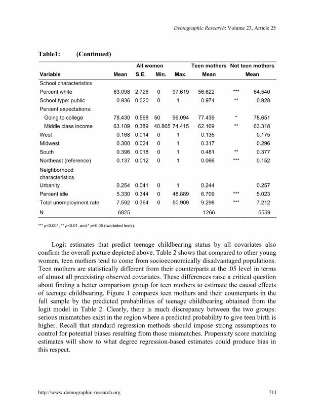
All women Teen mothers Not teen mothers Variable Mean S.E. Min. Max. Mean Mean School characteristics Percent white 63.098 2.726 0 97.619 56.622 *** 64.540 School type: public 0.936 0.020 0 1 0.974 ** 0.928 Percent expectations: Going to college 78.430 0.568 50 96.094 77.439 * 78.651 Middle class income 63.109 0.389 40.865 74.415 62.169 ** 63.318 West 0.168 0.014 0 1 0.135 0.175 Midwest 0.300 0.024 0 1 0.317 0.296 South 0.396 0.018 0 1 0.481 ** 0.377 Northeast (reference) 0.137 0.012 0 1 0.066 *** 0.152
Neighborhood characteristics
Urbanity 0.254 0.041 0 1 0.244 0.257 Percent idle 5.330 0.344 0 48.889 6.709 *** 5.023 Total unemployment rate 7.592 0.364 0 50.909 9.298 *** 7.212
N 6825 1266 5559 *** p<0.001, ** p<0.01, and * p<0.05 (two-tailed tests).
Logit estimates that predict teenage childbearing status by all covariates also confirm the overall picture depicted above. Table 2 shows that compared to other young women, teen mothers tend to come from socioeconomically disadvantaged populations. Teen mothers are statistically different from their counterparts at the .05 level in terms of almost all preexisting observed covariates. These differences raise a critical question about finding a better comparison group for teen mothers to estimate the causal effects of teenage childbearing. Figure 1 compares teen mothers and their counterparts in the full sample by the predicted probabilities of teenage childbearing obtained from the logit model in Table 2. Clearly, there is much discrepancy between the two groups: serious mismatches exist in the region where a predicted probability to give teen birth is higher. Recall that standard regression methods should impose strong assumptions to control for potential biases resulting from those mismatches. Propensity score matching estimates will show to what degree regression-based estimates could produce bias in this respect.

Lee: The early socioeconomic effects of teenage childbearing: A propensity score matching approach
712 http://www.demographic-research.org
Table 2: Odd ratios from logit model predicting teenage childbearing status
Coefficient S.E. Demographic and family characteristics Age at Wave I 0.899 ** (0.029) White (reference) Black 1.886 *** (0.207) Hispanic 1.986 *** (0.276) Asian 1.318 (0.285) Immigrant generation: 1st 0.347 *** (0.089) 2nd 0.632 ** (0.113) 3rd+ (reference) Two-biological parent family (reference)
Step family 1.697 *** (0.156) Mother only family 1.460 *** (0.140) Father only family 1.004 (0.186) Other family structure 1.915 ** (0.443) Parental education: Less than high school 2.049 *** (0.260) High school graduate 1.800 *** (0.163) Some college 1.616 *** (0.147) College graduate (reference) Number of siblings 1.040 (0.037)
Individual characteristics Parental monitoring 1.011 (0.026) Add Health PVT score 0.987 *** (0.003) Grade Point Average (GPA) 0.665 *** (0.034) Rotter/Rosenberg scale 0.755 *** (0.060) Religiosity 0.985 (0.034) Regular smoking 2.354 *** (0.190) Frequency of drinking 1.005 (0.010)
School characteristics Percent white 0.999 (0.002) School type: public 1.325 (0.227) Percent expectations: Going to college 0.978 * (0.011) Middle class income 1.021 (0.018)

Demographic Research: Volume 23, Article 25
Table 2: (Continued)
Coefficient S.E. West 1.539 * (0.330) Midwest 1.772 ** (0.347) South 2.198 *** (0.444) Northeast (reference)
Neighborhood characteristics Urbanity 0.866 (0.109) Percent idle 1.011 (0.008) Total unemployment rate 1.019 * (0.009)
-2 log pseudolikelihood 5256.063 N 6825
Notes: Missing indicators for parental education and Add Health PVT score are included but not shown; Robust standard errors
adjusting school-level clustering in parentheses. *** p<0.001, ** p<0.01, and * p<0.05 (two-tailed tests).
Figure 1: Predicted probability of teenage childbearing: Full sample
http://www.demographic-research.org 713

Lee: The early socioeconomic effects of teenage childbearing: A propensity score matching approach
5.2. Matching results
I construct a matched sample based on the estimated propensity scores of teenage childbearing. The matched sample consists of 1,259 teen mothers and 1,259 young women who are not teen mothers but whose propensity scores are sufficiently close to those of teen mothers. Figure 2 depicts the degree to which teen mothers and their matched counterparts overlap with each other. Strikingly, these two groups are well matched, indicating that there is little difference in the preexisting observed covariates.11
Figure 2: Predicted probability of teenage childbearing: Matched sample
11 In Appendix B, Table B gives an additional snapshot of the covariate balance check. None of the preexisting covariates bears statistical differences in means between teen mothers and their matched counterparts; the matched sample also achieves a significant percentage reduction in absolute bias. Although three variables - father only family, parents with some college education, and Midwest - show an increase in absolute bias (-22.3, -7710.3, and -173.4, respectively), these variables do not statistically differ between teen mothers and those who are not teen mothers before as well as after matching. Using the outcome-specific matched samples produces almost the same pattern of overlapping and covariate balance between these two groups (not shown).
714 http://www.demographic-research.org

Demographic Research: Volume 23, Article 25
http://www.demographic-research.org 715
Table 3 presents propensity score matching results of the socioeconomic effects of teenage childbearing. The first and second columns of each panel report the standard regression and propensity score matching estimates, respectively, for each outcome. The regression estimates are obtained from logit or OLS models using the full sample, including teenage childbearing status and all covariates in Table 2 as the explanatory variables. They are expressed as the simulated predicted probabilities or values computed by averaging each respondent’s value on all covariates except for teenage childbearing status. The matching estimates are the simple mean probabilities or values of each outcome in the matched sample. To make these two estimates comparable, the ratios between the treatment and control groups for each outcome are presented in the fourth rows of each panel.
As presented in the last rows of each panel, all outcome-specific matched samples have strong common support, ranging from 99.4% to 99.8%. This indicates that the propensity score matching method succeeds in locating almost all young women who are not teen mothers but share similar preexisting observed characteristics with teen mothers.
Table 3: Propensity score matching estimates of the effects of teenage childbearing
Regression Matching Regression Matching Estimates Estimates Estimates Estimates A. Educational attainment A1. Dropout A2. College attendance Not teen mothers (Control) 0.011 0.091 0.640 0.394 Teen mothers (Treatment) 0.104 0.180 0.185 0.239 Difference (T - C) 0.093 *** 0.089 *** -0.455 *** -0.155 *** Ratio (T/C) 9.455 1.978 0.289 0.606 Treatment cases 1263 1257 1257 1250 Control cases 5552 1257 5535 1250 Percent common support 99.5% 99.4%

Lee: The early socioeconomic effects of teenage childbearing: A propensity score matching approach
716 http://www.demographic-research.org
Table 3: (Continued)
Regression Matching Regression Matching Estimates Estimates Estimates Estimates B. Labor market outcomes
B1. Employment status B2. Work-related activities Not teen mothers (Control) 0.760 0.675 0.778 0.717 Teen mothers (Treatment) 0.572 0.570 0.639 0.633 Difference (T - C) -0.188 *** -0.105 *** -0.139 *** -0.084 ** Ratio (T/C) 0.753 0.845 0.821 0.883 Treatment cases 997 991 996 990 Control cases 3021 991 3018 990 Percent common support 99.4% 99.4%
B3. Full-time employment B4. Weekly wages (logged) Not teen mothers (Control) 0.840 0.830 5.883 5.824 Teen mothers (Treatment) 0.760 0.752 5.829 5.830 Difference (T - C) -0.080 *** -0.078 ** -0.054 0.006 Ratio (T/C) 0.905 0.906 0.991 1.001 Treatment cases 565 564 417 416 Control cases 2239 564 1802 416 Percent common support 99.8% 99.8% C. Public assistance receipt
C1. Currently on welfare C2. Ever on welfare Not teen mothers (Control) 0.038 0.109 0.053 0.101 Teen mothers (Treatment) 0.263 0.287 0.339 0.352 Difference (T - C) 0.225 *** 0.178 *** 0.286 *** 0.251 *** Ratio (T/C) 6.921 2.633 6.396 3.485 Treatment cases 1259 1252 1234 1228 Control cases 5538 1252 5453 1228 Percent common support 99.4% 99.5%
Note: Statistical significance levels calculated from bootstrap standard errors for the matched sample (300 replications). *** p<0.001, ** p<0.01, and * p<0.05 (two-tailed tests).
With respect to educational attainment, Panel A1 shows that when taking the ratio of the dropout rates between teen mothers and their matched counterparts, teen mothers are about two times more likely to be high school dropouts. This propensity score

Demographic Research: Volume 23, Article 25
http://www.demographic-research.org 717
matching estimate is less than a fourth of the logit estimate (=9.455) but still statistically significant. Panel A2 shows that teen mothers are about 40% less likely to attend or graduate from some college than their matched counterparts (1–.606=.394), which is an estimate that is much smaller than the logit estimate but remains statistically significant.
For labor market outcomes, the matching estimates also find the statistically significant negative effects of teenage childbearing, although the magnitudes of its effects are reduced compared to the logit estimates. Panels B1 through B4 show that compared to their matched counterparts, teen mothers are about 15% less likely to be employed, about 12% less likely to participate in work-related activities, and about 10% less likely to work full-time. The logit estimates for each labor market outcome are about 25%, 18%, and 10%, respectively. Weekly wages do not differ between teen mothers and their matched control group, but it should be noted that the analytic sample consists only of those who worked full-time, implying that this sample includes a select group of teen mothers.
The matching estimates presented in Panels C1 and C2 suggest that teen mothers are more likely than their matched counterparts to receive public assistance. While these estimates are far smaller than the logit estimates, teen mothers are still about 2.6 times and 3.5 times more likely to be currently and ever on welfare, respectively.
Overall, the propensity score matching results show that traditional regression methods tend to overestimate the negative effects of teen motherhood. Teen mothers’ lower levels of educational and labor market performance and higher likelihood of receiving public assistance result nontrivially from their preexisting disadvantages; and yet, there remain significant differences between teen mothers and their matched counterparts in the key domains of early socioeconomic outcomes. What is worth mentioning is that teen motherhood has relatively smaller effects on early labor market outcomes than on educational attainment and public assistance receipt. This result is not surprising, because the analytic samples for the labor market outcomes include a select group of teen mothers while excluding other young women enrolled in post-secondary schools, a group that has better economic potential. The matching results, therefore, suggest that even faced with the similarly adverse conditions when growing up, young women who are not teen mothers fare better than teen mothers.12
However, the matching estimates reported here do not take into account selection bias on unobserved preexisting characteristics, which may produce upwardly biased estimates. A contribution of this article is to conduct a sensitivity analysis using the
12 I reestimated the propensity score matching model where a young woman is treated as a teen mother if she gave birth prior to age 18 rather than 20 (see Appendix C). It does not alter the findings reported here, with the exception that the effects of teenage childbearing on the labor market outcomes become a little weaker.

Lee: The early socioeconomic effects of teenage childbearing: A propensity score matching approach
718 http://www.demographic-research.org
Rosenbaum bounds method to address the role of unobserved heterogeneity in drawing a causal inference about teen motherhood and its socioeconomic consequences.
5.3 Results from the sensitivity analysis
Table 4 presents the Rosenbaum bounds for the causal effects of teenage childbearing. Γ is the Rosenbaum bounds estimate of the magnitude of selection bias on unobserved covariate - hidden bias - that would predict teenage childbearing status, expressed as an odds ratio (OR). p-critical denotes the p-value at which a matching estimate becomes insignificant corresponding to the given magnitude of hidden bias. To give a substantive interpretation of the Rosenbaum bounds, I compare the magnitude of hidden bias (Γ) to that of its known equivalents. For example, parental decision-making on residence may be considered an important unmeasured factor of the relationship between teen motherhood and subsequent outcomes. One could argue that parental preference for middle-class neighborhood has a negative effect on daughters’ teenage childbearing and positive effects on their socioeconomic outcomes, because it signifies levels of parental investment in their children. If a researcher takes such family-level residential decision-making processes into account, the effects of teenage childbearing may disappear. Recall that consistent with previous research, the logit estimates from Table 2 confirm race/ethnicity, family structure, and parental education as among the strongest predictors of teenage childbearing status (Wu and Martinson 1993; Wu and Wolfe 2001). Then the question is how large the effect of parental residential preference should be to nullify the propensity score matching estimates, compared to that of these known characteristics.
Table 4: A sensitivity analysis using the Rosenbaum bounds of the causal
effects of teenage childbearing
Γ p-critical A. Educational Attainment Dropout 1.6 0.002 1.7 0.007 1.8 0.023 1.9 0.057 College attendance 1.7 0.002 1.8 0.010 1.9 0.039 2.0 0.110

Demographic Research: Volume 23, Article 25
http://www.demographic-research.org 719
Table 4: (Continued)
Γ p-critical B. Labor Market Outcomes Employment status 1.1 <0.001 1.2 0.003 1.3 0.028 1.4 0.133 Work-related activities 1.1 0.002 1.2 0.024 1.3 0.125 Full-time employment 1.1 0.005 1.2 0.023 1.3 0.072 Weekly wages (logged) 1.0 0.592 C. Public Assistance Receipt Currently on welfare 2.5 0.005 2.6 0.013 2.7 0.029 2.8 0.056 Ever on welfare 3.6 0.013 3.7 0.023 3.8 0.037 3.9 0.059
Notes: Γ is the odds ratio of differential treatment assignment due to an unobserved covariate; p-critical from the Wilcoxon signed
rank tests.
First, Panel A reports that as Γ approaches 1.9, the effect of teen motherhood on
dropping out of high school becomes statistically insignificant at the .05 level (p-critical is .057). This means that in order to challenge the significance of the matching estimate, an unobserved covariate should cause the odds ratio of teen motherhood to differ between teen mothers and their matched counterparts by a factor of 1.9. A selection bias with such magnitude is larger than or comparable to the estimated net effect of living in a step (OR=1.697) or a single mother (OR=1.460) family instead of a two-biological parent family, or having parents with a high school (OR=1.800) or some college

Lee: The early socioeconomic effects of teenage childbearing: A propensity score matching approach
720 http://www.demographic-research.org
(OR=1.616) education instead of a college diploma. To drive the effect of teenage childbearing on dropping out of high school to statistical insignificance, the effect of parental residential preference should be stronger than these effects even after controlling for all preexisting covariates included in Table 2.
With regard to attending or graduating from some college, the Rosenbaum bounds statistics indicates that Γ should be at least 2.0 (p-critical is .110) to completely alter the effect of teenage childbearing. The effect of parental residential preference should be larger than or comparable to the estimated net effect of being non-Hispanic black (OR=1.886) or Hispanic (OR=1.986) instead of being non-Hispanic white, living in another family structure instead of a two-biological parent family (OR=1.915), or having parents with less than high school diplomas instead of college diplomas (OR=2.049).
Second, the causal effects of teenage childbearing on labor market outcomes appear to be somewhat vulnerable to unobserved confounder, compared to educational attainment. Panel B suggests that to nullify the effects of teen motherhood on employment status, work-related activities, and full-time/part-time status, the critical values of Γ should be 1.4, 1.3, and 1.3 (p-criticals are .133, .125, and .072), respectively. The effect of teenage childbearing on weekly wages is highly vulnerable to hidden bias, which is consistent with the matching result shown in Table 3 that finds no effect. As Diprete and Gangl (2004) have pointed out, however, these results are worst-case scenarios. Unless family-level residential preference had a powerful effect on both teen motherhood and the outcomes, the effect of teenage childbearing on some of the labor market outcomes would remain significant.
Lastly, the Rosenbaum bounds for public assistance receipt (Panel C) imply that Γ should be at least 2.8 and 3.9 (p-critical values are .056 and .059), respectively, in order to wipe out the matching estimates of the effects of teen motherhood on being currently and ever on welfare. Because these magnitudes are much larger than any of the effects of race/ethnicity, family structure, and parental education estimated from Table 2, the effect of an unobserved covariate needs to be very powerful.
In summary, the sensitivity analysis using the Rosenbaum bounds shows that selection bias due to unobserved covariates would have to be substantial to completely eliminate the matching estimates of the effects of teenage childbearing on most of the early socioeconomic outcomes considered in this analysis. This result also suggests that since the magnitude of this sort of bias is interpreted in comparison to that of already known family background factors, one should not rule out the possibility that unobserved heterogeneity may underlie the relationship between teen motherhood and its socioeconomic consequences.

Demographic Research: Volume 23, Article 25
http://www.demographic-research.org 721
5.4 Racial/ethnic differences
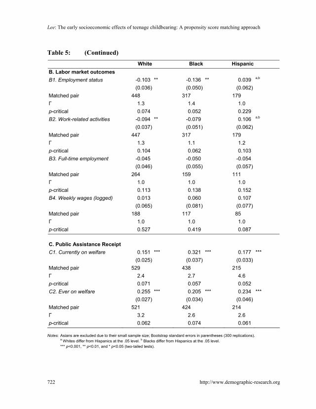
Given recent changes in the U.S. racial/ethnic composition (e.g., the increase of Hispanics) and the conflicting findings regarding the effects of teenage childbearing by race/ethnicity, an examination of racial/ethnic differences deserves attention.13 Table 5 reports the propensity score matching estimates among non-Hispanic whites, non-Hispanic blacks, and Hispanics. For non-Hispanic whites, the matching estimates show that teen motherhood has negative effects on educational attainment, employment status, work-related activities, and public assistance receipt, but not on full-time/part-time status and weekly wages. The Rosenbaum bounds suggest that the effects of teen motherhood on public assistance receipt and to a lesser degree, educational attainment are most robust to unobserved heterogeneity, compared to employment status and work-related activities. For non-Hispanic blacks, teen motherhood has adverse consequences on educational attainment, employment status, and public assistance receipt. For Hispanics, teen motherhood has negative effects on educational attainment and public assistance receipt. Although its effects on employment status and work-related activities are not significant, they differ significantly from those for non-Hispanic whites and blacks.
Table 5: Propensity score matching estimates of the effects of teenage
childbearing, by race/ethnicity White Black Hispanic A. Educational attainment A1. Dropout 0.075 *** 0.061 ** 0.077 * (0.024) (0.025) (0.036) Matched pair 533 445 222 Γ 1.5 1.4 1.3 p-critical 0.097 0.079 0.081 A2. College attendance -0.124 *** -0.161 *** -0.209 *** (0.029) (0.037) (0.047) Matched pair 533 441 220 Γ 1.7 1.8 2.3 p-critical 0.068 0.061 0.063
13 Grogger and Bronars (1993) report that most of the adverse consequences of teen motherhood are amplified among blacks, whereas Klepinger, Lundberg, and Plotnick (1999) find that the negative effects of teen motherhood are present for both whites and blacks.
Lee: The early socioeconomic effects of teenage childbearing: A propensity score matching approach
722 http://www.demographic-research.org
Table 5: (Continued)
White Black Hispanic B. Labor market outcomes B1. Employment status -0.103 ** -0.136 ** 0.039 a,b (0.036) (0.050) (0.062) Matched pair 448 317 179 Γ 1.3 1.4 1.0 p-critical 0.074 0.052 0.229 B2. Work-related activities -0.094 ** -0.079 0.106 a,b (0.037) (0.051) (0.062) Matched pair 447 317 179 Γ 1.3 1.1 1.2 p-critical 0.104 0.062 0.103 B3. Full-time employment -0.045 -0.050 -0.054 (0.046) (0.055) (0.057) Matched pair 264 159 111 Γ 1.0 1.0 1.0 p-critical 0.113 0.138 0.152 B4. Weekly wages (logged) 0.013 0.060 0.107 (0.065) (0.081) (0.077) Matched pair 188 117 85 Γ 1.0 1.0 1.0 p-critical 0.527 0.419 0.087 C. Public Assistance Receipt C1. Currently on welfare 0.151 *** 0.321 *** 0.177 *** (0.025) (0.037) (0.033) Matched pair 529 438 215 Γ 2.4 2.7 4.6 p-critical 0.071 0.057 0.052 C2. Ever on welfare 0.255 *** 0.205 *** 0.234 *** (0.027) (0.034) (0.046) Matched pair 521 424 214 Γ 3.2 2.6 2.6 p-critical 0.062 0.074 0.061
Notes: Asians are excluded due to their small sample size; Bootstrap standard errors in parentheses (300 replications).
a Whites differ from Hispanics at the .05 level. b Blacks differ from Hispanics at the .05 level. *** p<0.001, ** p<0.01, and * p<0.05 (two-tailed tests).

Demographic Research: Volume 23, Article 25
http://www.demographic-research.org 723
The results imply that teenage childbearing is detrimental to non-Hispanic whites and blacks, but less so to Hispanics. Insofar as labor market performance is concerned, the findings from Hispanic teen mothers seem in favor of the selection view (Geronimus, Korenman, and Hillemeier 1994). Alternatively, given a large number of respondents who were enrolled in post-secondary schools at Wave III (about 41% for non-Hispanic whites, 42% for non-Hispanic blacks, and 38% for Hispanics), the effects of teenage childbearing on the labor market outcomes might be restored if these respondents entered the labor market upon graduation. Since the economic returns to education have increased over the past 30 years (Card 1999; Lemieux 2006), significant difference in education attainment between teen mothers and their matched counterparts may be carried over into the labor market across all racial/ethnic groups. New data that contain older age groups would help determine which interpretation can be substantiated.
6. Discussion and conclusion
Studies of teenage childbearing and its socioeconomic consequences have been concerned about possible omitted variables and selection biases that are critical to estimate the “true” effect of teenage childbearing. The propensity score matching analysis used in this article is designed to shed new light into this line of research by 1) finding a better comparison group to teen mothers with less dependence on statistical assumptions than standard regression approaches and a larger sample size; 2) employing the Rosenbaum bounds method to assess the significance level of the matching estimates of the effects of teenage childbearing in the presence of selection bias on unobserved covariates; and 3) providing the most up-to-date assessment of the early socioeconomic effects of teenage childbearing with the Add Health data.
As in most of the previous studies taking alternative approaches, the propensity score matching results show that socioeconomic disadvantages inherent to teen mothers account for a nontrivial portion of the effects of teen motherhood, suggesting that the selection bias problem results in an overestimation of its negative effects. However, when teen mothers are compared to their matched counterparts who are similar in every observed preexisting characteristic except for teenage childbearing status, teen motherhood still has modest but significant negative effects on various early socioeconomic outcomes. The sensitivity analysis employing the Rosenbaum bounds method suggests that selection bias on unobserved covariates would have to be large to alter these propensity score matching estimates. These findings are consistent with some of the earlier studies using within-family fixed-effects models (Hoffman, Foster, and Furstenberg 1993a, 1993b; Holmlund 2005), instrumental variables methods
Lee: The early socioeconomic effects of teenage childbearing: A propensity score matching approach
724 http://www.demographic-research.org
(Klepinger, Lundberg, and Plotnick 1999), and quasi-natural experimental approaches (Grogger and Bronars 1993; Fletcher and Wolfe 2009). This convergence in the findings points out that identifying a more reliable comparison group to teen mothers through flexible modeling assumptions and well-supported data should be given a priority.
Several limitations of this study warrant mention. First, one should recognize that the propensity score matching analysis combined with the Rosenbaum bounds method is not a solution to resolve all complex issues regarding unobserved heterogeneity; rather, it need be understood as an effort to make the causal inference about teenage childbearing more constructive. Second, given the nature of the data, this study speaks to the effects of teenage childbearing on young adults. Some studies using miscarriages as a source of quasi-natural experiment report that teen mothers fare better in their late 20s (Hotz, McElroy, and Sanders 1997, 2005). Whether or not teen motherhood has long-term consequences, therefore, remains an important topic for future research. Third, it is likely that structural changes influence the association between teenage childbearing and subsequent outcomes, but this study is only suggestive of the potential roles of the growing economic returns to education. Research on adolescent fertility can benefit from more comprehensive knowledge about teen mothers’ life experiences, new data with older age groups, and cohort data linking teenage childbearing to macro-level social changes.
7. Acknowledgements
I thank Kathleen Mullan Harris, Sara McLanahan, Lawrence Wu, Robert Mare, Colter Mitchell, Amy Bailey, the Demographic Research associate editor Carl Schmertmann, and two anonymous reviewers for their insightful and helpful comments on earlier versions of this article. Any remaining errors or omissions are solely my own. This research uses data from Add Health, a program project designed by J. Richard Udry, Peter S. Bearman, and Kathleen Mullan Harris, and funded by a grant P01-HD31921 from the National Institute of Child Health and Human Development, with cooperative funding from 17 other agencies. Special acknowledgment is due Ronald R. Rindfuss and Barbara Entwisle for assistance in the original design. Persons interested in obtaining data files from Add Health should contact Add Health, Carolina Population Center, 123 W. Franklin Street, Chapel Hill, NC 27516-2524, USA ([email protected]).

Demographic Research: Volume 23, Article 25
http://www.demographic-research.org 725
References
An, C.-B., Haveman, R., and Wolfe, B. (1993). Teen out-of-wedlock births and welfare receipt: The role of childhood events and economic circumstances. Review of Economics and Statistics 75(2): 195-208. doi:10.2307/2109424.
Angrist, J.D. and Krueger, A.B. (2001). Instrumental variables and the search for identification: From supply and demand to natural experiments. Journal of Economic Perspectives 15(4): 69-85. doi:10.1257/jep.15.4.69.
Becker, G. (1993). Human Capital: A Theoretical and Empirical Analysis, with Special Reference to Education. Chicago, IL: University of Chicago Press.
Cameron, S.V. and Heckman, J.H. (1993). The nonequivalence of high school equivalents. Journal of Labor Economics 11(1): 1-47. doi:10.1086/298316.
Cao, J., Stromsdorfer, E.W., and Weeks, G. (1996). The human capital effect of general education development certificates on low income women. The Journal of Human Resources 31(1): 206-228. doi:10.2307/146048.
Card, D. (1999). The causal effect of education on earnings. In: Ashenfelter, O. and Card, D. (eds.). Handbook of Labor Economics, vol. 3. Amsterdam, Netherland: Elsevier.
Cherlin, A.J. (2001). New Developments in the Study of Nonmarital Childbearing. In: Wu, L.L. and Wolfe, B. (eds.). Out of Wedlock: Causes and Consequences of Nonmarital Fertility. New York, NY: Russell Sage Foundation: 390-402.
Chevalier, A. and Viitanen, T.K. (2003). The long-run labour market consequences of teenage motherhood in Britain. Journal of Population Economics 16(2): 323-343. doi:10.1007/s001480200125.
Coleman, J. (1990). Foundations of Social Theory. Cambridge, MA: Harvard University Press.
Dehejia, R.H. and Wahba, S. (2002). Propensity score matching methods for nonexperimental causal studies. Review of Economics and Statistics 84(1): 151-161. doi:10.1162/003465302317331982.
DiPrete, T.A. and Gangl, M. (2004). Assessing bias in the estimation of causal effects: Rosenbaum bounds on matching estimators and instrumental variables estimation with imperfect instruments. Sociological Methodology 34(1): 271-310. doi:10.1111/j.0081-1750.2004.00154.x.

Lee: The early socioeconomic effects of teenage childbearing: A propensity score matching approach
726 http://www.demographic-research.org
Fletcher, J.M. and Wolfe, B. (2009). Education and labor market consequences of teenage childbearing: Evidence using the timing of pregnancy: Outcomes and community fixed effects. Journal of Human Resources 44(2): 303-325.
Furstenberg, F.F.Jr. (1991). As the pendulum swings: Teenage childbearing and social concern. Family Relations 40(2): 127-138. doi:10.2307/585470.
Geronimus, A.T. (1991). Teenage childbearing and social and reproductive disadvantage: The evolution of complex questions and the demise of simple answers. Family Relations 40(4): 463-471. doi:10.2307/584905.
Geronimus, A.T. and Korenman, S. (1992). The socioeconomic consequences of teenage childbearing reconsidered. Quarterly Journal of Economics 107(4): 1187-1214. doi:10.2307/2118385.
Geronimus, A.T. and Korenman, S. (1993). The socioeconomic costs of teenage childbearing: Evidence and interpretation. Demography 30(2): 281-290. doi:10.2307/2061842.
Geronimus, A.T., Korenman, S., and Hillemeier, M.M. (1994). Does young maternal age adversely affect child development? Evidence from cousin comparisons in the United States. Population and Development Review 20(3): 585-609. doi:10.2307/2137602.
Grogger, J. and Bronars, S. (1993). The socioeconomic consequences of teenage childbearing: Findings from a natural experiment. Family Planning Perspectives 25(4): 156-161+174. doi:10.2307/2135923.
Harding, D.J. (2003). Counterfactual models of neighborhood effects: The effect of neighborhood poverty on dropping out and teenage pregnancy. American Journal of Sociology 109(3): 676-719. doi:10.1086/379217.
Harris, K.M., Halpern, C.T., Whitsel, E., Hussey, J., Tabor, J., Entzel, P., and Udry, J.R. (2009). The National Longitudinal Study of Adolescent Health: Research design [electronic source]. Chapel Hill, NC: Carolina Population Center. http://www.cpc.unc.edu/projects/addhealth/design.
Heckman, J.J., Ichimura, H., and Todd, P. (1998). Matching as an econometric evaluation estimator. Review of Economic Studies 65(2): 261-294. doi:10.1111/1467-937X.00044.
Heckman, J., Stixrud, J., and Urzua, S. (2006). The effects of cognitive and noncognitive abilities on labor market outcomes and Social behavior. (NBER Working Paper No. 12006).

Demographic Research: Volume 23, Article 25
http://www.demographic-research.org 727
Hofferth, S. and Hayes, C. (1987). Risking the Future. Washington, DC: National Academy Press.
Hoffman, S.D. (1998). Teenage childbearing is not so bad after all… Or is it? A review of the new literature. Family Planning Perspectives 30(5): 236-239&243.
Hoffman, S.D., Foster, E.M., and Furstenberg, F.F.Jr. (1993a). Reevaluating the costs of teenage childbearing. Demography 30(1): 1-13. doi:10.2307/2061859.
Hoffman, S.D., Foster, E.M., and Furstenberg, F.F.Jr. (1993b). Reevaluating the costs of teenage childbearing: Response to Geronimus and Korenman. Demography 30(2): 291-296. doi:10.2307/2061843.
Holland, P.W. (1986). Statistics and causal inference. Journal of the American Statistics Association 81(396): 945-960. doi:10.2307/2289064.
Holmlund, H. (2005). Estimating Long-Term Consequences of Teenage Childbearing: An Examination of the Siblings Approach. Journal of Human Resources 40(3):716-743.
Hotz, V.J., McElroy, S.W., and Sanders, S.G. (1997). The costs and consequences of teenage childbearing for the mothers and the government. In: Maynard, R.A. (ed.). Kids Having Kids. Washington, DC: The Urban Institute Press: 55-94.
Hotz, V.J., McElroy, S.W., and Sanders, S.G. (2005). Teenage childbearing and its life cycle consequences: Exploiting a natural experiment. Journal of Human Resources 40(3): 683-715. doi:10.3386/w7397.
Imbens, G.W. and Angrist, J.D. (1994). Identification and estimation of local average treatment effects. Econometrica 62(2): 467-475. doi:10.2307/2951620.
Klepinger, D., Lundberg, S., and Plotnick, R. (1999). How does adolescent fertility affect the human capital and wages of young women? Journal of Human Resources 34(3): 421-448. doi:10.2307/146375.
Korenman, S., Kaestner, R., and Joyce, T.J. (2001). Unintended pregnancy and the consequences of nonmarital childbearing. In: Wu, L.L. and Wolfe, B. (eds.). Out of Wedlock: Causes and Consequences of Nonmarital Fertility. New York: Russell Sage Foundation: 259-286.
Lemieux, T. (2006). Increasing residual wage inequality: Composition effects, noisy data, or rising demand for skill? American Economic Review 96(3): 461-498. doi:10.1257/aer.96.3.461.

Lee: The early socioeconomic effects of teenage childbearing: A propensity score matching approach
728 http://www.demographic-research.org
Levine, D.I. and Painter, G. (2003). The schooling costs of teenage out-of-wedlock childbearing: Analysis with a within-school propensity-score-matching estimator. Review of Economics and Statistics 85(4): 884-900. doi:10.1162/003465303772815790.
Martin, J.A., Hamilton, B.E., Sutton, P.D., Ventura, S.J., Menacker, F., and Kirmeyer, S. (2006). Births: Final data for 2004. National Vital Statistics Reports 55(1). (Hyattsville, MD: National Center for Health Statistics).
Massey, D. and Denton, N. (1993). American Apartheid. Cambridge, MA: Harvard University Press.
Morgan, S.L. (2001). Counterfactuals, causal effect heterogeneity, and the catholic school effect on learning. Sociology of Education 74(4): 341-374. doi:10.2307/2673139.
Morgan, S.L. and Harding, D.J. (2006). Matching estimators of causal effects: Prospects and pitfalls in theory and practice. Sociological Methods and Research 35(1): 3-60. doi:10.1177/0049124106289164.
Morgan, S.L. and Winship, C. (2007). Counterfactuals and Causal Inference: Methods and Principles for Social Research. New York, NY: Cambridge University Press.
Morris, M. and Western, B. (1999). Inequality in earnings at the close of the twentieth century. Annual Review of Sociology 25: 623-657. doi:10.1146/ annurev.soc.25.1.623.
Olsen, R.J. and Farkas, G. (1989). Endogenous covariates in duration models and the effect of adolescent childbirth on schooling. Journal of Human Resources 24(1): 39-53. doi:10.2307/145932.
Ribar, D.C. (1994). Teenage fertility and high school completion. Review of Economics and Statistics 76(3): 413-424. doi:10.2307/2109967.
Rindfuss, R.R. (1991). The young adult years: Diversity, structural change, and fertility. Demography 28(4): 493-512. doi:10.2307/2061419.
Rosenbaum, P.R. (2002). Observational Studies. New York, NY: Springer.
Rosenbaum, P.R. and Rubin, D.B. (1983). The central role of the propensity score in observational studies for causal effects. Biometrika 70(1): 41-55. doi:10.1093/biomet/70.1.41.

Demographic Research: Volume 23, Article 25
http://www.demographic-research.org 729
Rosenberg, M. (1965). Society and the Adolescent Self-Image. Princeton, NJ: Princeton University Press.
Rotter, J. (1966). Generalized expectancies for internal versus external control of reinforcement. In: Rotter, J., Chance, J., and Phares, E. (eds.). Applications of a Social Learning Theory of Personality. New York, NY: Holt, Rinehart and Winston, Inc: 260-295.
Rubin, D.B. (1977). Assignment to a treatment group on the basis of a covariate. Journal of Educational Statistics 2(1): 1-26. doi:10.2307/1164933.
Udry, J.R. and Chantala, K. (2003). Missing school dropouts in surveys does not bias risk estimates. Social Science Research 32(2): 294-311. doi:10.1016/S0049-089X(02)00060-1.
Upchurch, D.M. and McCarthy, J. (1990). The timing of a first birth and high school completion. American Sociological Review 55(2): 224-234. doi:10.2307/2095628.
Ventura, S., Abma, J.C., Mosher, W.D., and Henshaw, S. (2004). Estimated pregnancy rates for the United States, 1990-2000: An update. National Vital Statistics Reports 52(23): 1-9. (Hyattsville, MD: National Center for Health Statistics).
Wilson, W. (1987). The Truly Disadvantaged. Chicago, IL: University of Chicago Press.
Winship, C. and Mare, R.D. (1992). Models for sample selection bias. Annual Review of Sociology 18: 327-350. doi:10.1146/annurev.so.18.080192.001551.
Winship, C. and Morgan, S.L. (1999). The estimation of causal effects from observational data. Annual Review of Sociology 25: 659-706. doi:10.1146/ annurev.soc.25.1.659.
Wu, L.L. and Martinson, B.C. (1993). Family structure and the risk of a premarital birth. American Sociological Review 58(2): 210-232. doi:10.2307/2095967.
Wu, L. and Wolfe, B. (2001). Out of Wedlock: Causes and Consequences of Nonmarital Fertility. New York, NY: Russell Sage Foundation.

Lee: The early socioeconomic effects of teenage childbearing: A propensity score matching approach
Appendix A: The Rosenbaum bounds method
The Rosenbaum bounds method is complementary to the estimation of treatment effects using data on matched pairs (Rosenbaum 2002). Although Rosenbaum developed the theory for a more general case, I limit the focus to his treatment of the case of matched pairs (see Chapter 4 of Rosenbaum (2002) and DiPrete and Gangl (2004) for more details).
Test statistics in the family of sign score statistics have the form
(A.1) ∑ ∑= =
==S
s isisis ZcdrZtT
1
2
1,),(
where Z is the variable that designates which of each of the s pairs was treated, and r measures the outcome for each case in the S pairs. Zsi equals 1 if a case is treated, and 0 otherwise; c is defined as follows:
. if 0 ,0, if 1 ,0, if 0 ,1
2121
2121
2121
ssss
ssss
ssss
rrccrrccrrcc
===<==>==
Finally, ds is the rank of |rs1 – rs2| with average ranks used for ties. The product of
the c and Z variables causes pairs to be selected where the outcome for the treatment was greater than the outcome for the control. The ranks of these cases are summed and compared with the distribution of the test statistic under the null hypothesis that the treatment has no effect.
In the case where the assignment to treatment is not random, the above test statistic can be bounded. It is assumed that there is an unmeasured variable, U, that affects the probability of receiving the treatment. If we let πi be the probability that the ith unit receives the treatment, and X is the vector of observed covariates that determine treatment and that also determine the outcome variable, then the following treatment assignment equation applies:
.10 where,)(1
log ≤≤+=⎟⎟⎠
⎞⎜⎜⎝
⎛− iii
i
i UUX γκπ
π (A.2)
730 http://www.demographic-research.org

Demographic Research: Volume 23, Article 25
Rosenbaum (2002) shows that this relationship implies the following bounds on the ratio of the odds that either of two cases which are matched on X—or alternatively on the propensity score p(X)—will receive the treatment
,)1()1(1
1,2,
2,1, Γ≤−
−≤
Γ ss
ss
ππππ
(A.3)
where s indexes the matched pair, s = 1,…,S, and Γ = exp(γ).
Under the assumption that a confounding variable U exists, equation (A.1) becomes the sum of S independent random variables where the sth pair equals ds with probability
)exp()exp()exp()exp(
21
2211
ss
sssss uu
ucucp
γγγγ
++
=
and equals 0 with probability 1 – ps. Define
⎪⎩
⎪⎨
⎧
≠
====
=⎪⎩
⎪⎨
⎧
≠
====
=
Γ+
−
Γ+Γ
+
. if ,1 if 1,0 if 0
and , if
,1 if 1,0 if 0
2111
21
21
211
21
21
ss
ss
ss
s
ss
ss
ss
s
cccccc
pcccccc
p
Rosenbaum (2002) shows that for any specific γ, the null distribution of t(Z,r) is bounded by two known distributions for T+ and T– that are attained at values of U, which perfectly predict the signs of csi in equation (A.1), where
).1()var( and )(
),1()var( and )(
1 1
2
1 1
2
−
= =
−−−−
+
= =
++++
∑ ∑
∑ ∑
−==
−==
s
S
s
S
sssss
s
S
s
S
sssss
ppdTpdTE
ppdTpdTE
One can use these formulae to compute the significance level of the null hypothesis of no treatment effect. For any specific Γ, we compute
)var(/))(( and )var(/))(( −−++ −− TTETTTET
where T is the Wilcoxon signed rank statistic. These two values give bounds of the significance level of a one-sided test for no treatment effect.
http://www.demographic-research.org 731
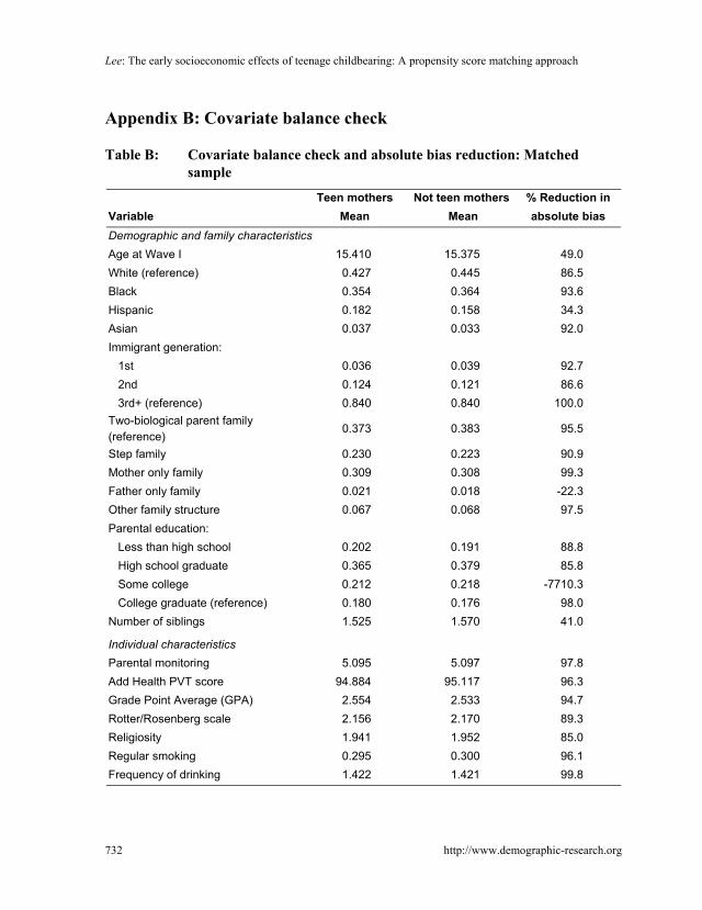
Lee: The early socioeconomic effects of teenage childbearing: A propensity score matching approach
732 http://www.demographic-research.org
Appendix B: Covariate balance check
Table B: Covariate balance check and absolute bias reduction: Matched sample
Teen mothers Not teen mothers % Reduction in Variable Mean Mean absolute bias Demographic and family characteristics Age at Wave I 15.410 15.375 49.0 White (reference) 0.427 0.445 86.5 Black 0.354 0.364 93.6 Hispanic 0.182 0.158 34.3 Asian 0.037 0.033 92.0 Immigrant generation: 1st 0.036 0.039 92.7 2nd 0.124 0.121 86.6 3rd+ (reference) 0.840 0.840 100.0 Two-biological parent family (reference)
0.373 0.383 95.5
Step family 0.230 0.223 90.9 Mother only family 0.309 0.308 99.3 Father only family 0.021 0.018 -22.3 Other family structure 0.067 0.068 97.5 Parental education: Less than high school 0.202 0.191 88.8 High school graduate 0.365 0.379 85.8 Some college 0.212 0.218 -7710.3 College graduate (reference) 0.180 0.176 98.0 Number of siblings 1.525 1.570 41.0
Individual characteristics Parental monitoring 5.095 5.097 97.8 Add Health PVT score 94.884 95.117 96.3 Grade Point Average (GPA) 2.554 2.533 94.7 Rotter/Rosenberg scale 2.156 2.170 89.3 Religiosity 1.941 1.952 85.0 Regular smoking 0.295 0.300 96.1 Frequency of drinking 1.422 1.421 99.8

Demographic Research: Volume 23, Article 25
http://www.demographic-research.org 733
Table B: (Continued)
Teen mothers Not teen mothers % Reduction in Variable Mean Mean absolute bias School characteristics Percent white 50.241 51.661 76.2 School type: public 0.969 0.973 92.7 Percent expectations: Going to college 77.617 77.601 98.9 Middle class income 62.152 62.045 91.0 West 0.214 0.200 66.6 Midwest 0.237 0.230 -173.4 South 0.474 0.490 85.7 Northeast (reference) 0.075 0.079 94.2 Neighborhood characteristics Urbanity 0.255 0.249 81.6 Percent idle 6.323 6.093 82.1 Total unemployment rate 9.033 9.159 92.7
N 1259 1259

Lee: The early socioeconomic effects of teenage childbearing: A propensity score matching approach
734 http://www.demographic-research.org
Appendix C: Teenage childbearing defined as giving birth before age 18
Table C: Propensity score matching estimates of the effects of teenage childbearing
Regression Matching Regression Matching Estimates Estimates Estimates Estimates
A. Educational Attainment A1. Dropout A2. College attendance Not teen mothers (Control) 0.014 0.094 0.589 0.411 Teen mothers (Treatment) 0.144 0.229 0.182 0.241 Difference (T - C) 0.130 *** 0.135 *** -0.406 *** -0.170 *** Ratio (T/C) 10.286 2.436 0.310 0.585 Treatment cases 575 572 573 569 Control cases 6240 572 6219 569 Percent common support 99.5% 99.3% B. Labor Market Outcomes B1. Employment status B2. Work-related activities Not teen mothers (Control) 0.735 0.641 0.759 0.670 Teen mothers (Treatment) 0.555 0.552 0.636 0.627 Difference (T - C) -0.180 *** -0.089 * -0.123 * -0.042 Ratio (T/C) 0.755 0.861 0.838 0.937 Treatment cases 453 449 452 448 Control cases 3565 449 3562 448 Percent common support 99.1% 99.1%
B3. Full-time employment B4. Weekly wages (logged) Not teen mothers (Control) 0.832 0.847 5.877 5.723 Teen mothers (Treatment) 0.747 0.738 5.825 5.834 Difference (T - C) -0.085 -0.109 * -0.052 0.111 Ratio (T/C) 0.898 0.871 0.991 1.019 Treatment cases 250 248 182 178 Control cases 2554 248 2037 178 Percent common support 99.2% 97.8%

Demographic Research: Volume 23, Article 25
http://www.demographic-research.org 735
Table C: (Continued)
Regression Matching Regression Matching Estimates Estimates Estimates Estimates
C. Public Assistance Receipt C1. Currently on welfare C2. Ever on welfare Not teen mothers (Control) 0.052 0.145 0.074 0.168 Teen mothers (Treatment) 0.285 0.310 0.341 0.356 Difference (T - C) 0.233 *** 0.165 *** 0.267 *** 0.188 *** Ratio (T/C) 5.481 2.139 4.608 2.122 Treatment cases 571 567 567 564 Control cases 6226 567 6120 564 Percent common support 99.3% 99.5%
Note: Statistical significance levels calculated from bootstrap standard errors for the matched sample (300 replications).
*** p<0.001, ** p<0.01, and * p<0.05 (two-tailed tests).

Lee: The early socioeconomic effects of teenage childbearing: A propensity score matching approach
736 http://www.demographic-research.org