the earnings estimate dispersion effect in international ... · the earnings estimate dispersion...

15.05.2009 QST1

Harald Lohre, Union InvestmentMarkus Leippold, University of Zurich

Venice, June 1, 2009

The Earnings Estimate Dispersion Effect in International Stock Returns

Northfield’s 22nd Annual Research Conference

Outline

15.05.2009 QST2

1 Motivation and Data

2 Traditional Analysis of the Dispersion Effect

3 The Dark Side of Statistics: Data Snooping

4 Rationalizing the Dispersion Effect

5 Conclusion

The Dispersion Effect

Besides the mean, the distribution of earnings forecasts may contain additional valuable information

The dispersion of earnings forecasts helps judging the credibility of a given earnings signal

While intuition suggests a risk premium for bearing more uncertain earnings prospects, empirical evidence is at odds with dispersion being a priced risk factor

Diether, Malloy, and Scherbina (2002) contend:

– Dispersion is not a risk factor but rather a metric for differences of opinion

– Prices tend to reflect the view of the optimists whenever there is disagreement since the pessimists' views are not revealed due to short-sale constraints (Miller, 1977)

15.05.2009 QST3


Motivation of our Paper

Does the dispersion effect extend to European markets?

Rationalizing a given anomaly is only meaningful if the evidence is not spurious in the first place

When internationally investigating the dispersion effect we address the following issues:

– Traditional Risk and Return Analysis

– Robustness with respect to data snooping?

– The role of information uncertainty

– The role of liquidity risk

– Is the anomaly persistent or being exploited?

15.05.2009 QST4


Motivation (cont'd)

15.05.2009 QST5

The need for robustness checks

– In some cases, anomalies might be more apparent than real.

– A common strategy for robustness checks is to study trading strategies in many countries or for different time periods.

– In our paper, we choose to study the dispersion effect in different countries.

But with the right tools!

– Researchers have long been aware of data snooping biases (Lo and MacKinlay, 1990; Sullivan et al., 1999; White, 2000).

– Common statistical procedures are rarely optimal in terms of power, hence most likely rejecting the anomaly.

– To overcome these problems, we make use of latest results on multiple hypotheses testing.


Data and Sample Selection

Comprehensive sample of 16 developed countries:

– 15 European markets and the U.S., spanning 1987-2009.

– Largest European markets: U.K., France, Germany, Switzerland and the Netherlands.

– Survivorship bias avoided by including dead companies.

– Adjust for secondary issues and cross-listings.

– Penny stocks are excluded, i.e., stock price below $5.

– In total, we end up with 59,394 firm-years (32,905 firm-years for the U.S.).

Cleaning Datastream Return Data:

– Ince and Porter (2006), “Handle Datastream Data with Care!“

– Issues not resolved by Datastream have been screened and corrected.

15.05.2009 QST6


Outline

15.05.2009 QST7





5 Conclusion

The Dispersion Strategy

Following Diether, Malloy and Scherbina (2002) we define:

Based on the previous month‘s dispersion stocks are asssigned into

– Quintiles for larger countries

– Terciles for smaller countries

The dispersion strategy is to go long low dispersion stocks and to go short high dispersion stocks.

Holding period is one month

15.05.2009 QST8


Return and Volatility of Dispersion Portfolios

15.05.2009 QST9


Portfolio Dispersion Ranking

Country Low 2 Mid 4 High Lo-Hi t-stat

USA Return 1.22 0.87 0.87 0.82 0.72 0.50 2.05Volatility 4.98 5.08 5.64 6.33 7.49 3.93

Europe Return 0.88 0.76 0.74 0.62 0.45 0.43 2.46Volatility 4.21 4.64 4.97 5.22 5.96 2.81

Austria Return 1.08 0.69 0.50 0.58 2.31Volatility 6.30 6.27 6.41 4.06

Belgium Return 0.83 0.74 0.41 0.43 2.20Volatility 4.82 5.26 5.84 3.14

France Return 1.01 0.93 0.77 0.59 0.55 0.46 1.83Volatility 5.33 5.68 6.15 6.46 7.43 4.05

Germany Return 0.58 0.49 0.49 0.26 0.12 0.46 1.98Volatility 5.27 5.62 6.00 6.08 7.56 3.78

Italy Return 0.62 0.56 0.56 0.33 0.02 0.60 2.22Volatility 6.27 6.89 6.63 6.67 7.86 4.37

Netherlands Return 1.14 0.99 0.82 0.77 0.37 0.76 2.81Volatility 5.13 5.28 5.69 5.97 7.01 4.39

Spain Return 1.14 0.89 0.71 0.66 0.50 0.64 2.43Volatility 5.05 5.85 6.02 6.67 7.10 4.23

Characteristics of Dispersion Portfolios

15.05.2009 QST10


Prior U.S. evidence is confirmed (Diether, Malloy & Scherbina, 2002 orAvramov, Chordia, Jostova & Philipov, 2008) and the European experiencelooks promising as well.

The lion‘s share of the hedge returns is typically due to the high dispersionportfolio.

As for the quantile portfolios‘ dispersion we note that the high dispersionportfolio is decidedly different from the remaining portfolios in that there isconsiderable disagreement among analysts.

As a consequence the quantile portfolios‘ volatility increases with dispersion.

Moreover, we find the highest betas for the high dispersion portfolios, whichcalls for controlling for common risk factors in the hedge strategies‘ returns!

Are the dispersion strategies simply compensating for risk?

Fama-French-Momentum Regressions

15.05.2009 QST11


α β γ δ φ t(α) t(β) t(γ) t(δ) t(φ) Adj.R²

Low 0.11 0.94 -0.32 -0.02 0.18 1.03 41.66 -11.50 -0.54 3.56 88.2USA High -0.60 1.25 -0.05 -0.20 -0.28 -4.23 42.44 -1.28 -4.19 -4.24 91.6

Low-High 0.71 -0.31 -0.28 0.18 0.45 4.51 -9.55 -6.74 3.39 6.26 64.6

Low 0.00 0.96 -0.33 0.07 0.25 0.06 51.01 -13.11 2.00 5.27 92.5Europe High 0.01 1.27 -0.25 -0.10 -0.44 0.05 47.05 -7.11 -2.04 -6.38 92.7

Low-High 0.00 -0.32 -0.07 0.17 0.69 -0.01 -9.88 -1.66 2.89 8.46 55.1

Risk factors explain a sizeable portion of the hedge returns

Considerate negative market exposure indicates hedging potential

While the U.S. alpha is robust to the common factor controls, the European one is fully explained away, however, Austria, Italy, the Netherlands, and Spain are robust as well.

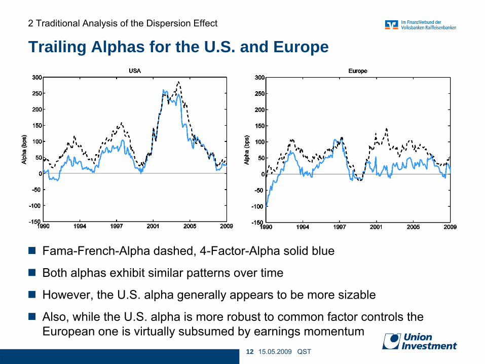
Trailing Alphas for the U.S. and Europe

15.05.2009 QST12


Fama-French-Alpha dashed, 4-Factor-Alpha solid blue

Both alphas exhibit similar patterns over time

However, the U.S. alpha generally appears to be more sizable

Also, while the U.S. alpha is more robust to common factor controls theEuropean one is virtually subsumed by earnings momentum

Outline

15.05.2009 QST13





5 Conclusion

Data Snooping and Anomalies

15.05.2009 QST14

When testing several strategies some may outperform by chance alone:

– Extensive re-use of a given database.

– Testing one investment idea in similar markets.

Control for data-snooping is essential:

– Goal: When assessing several strategies, avoid as many false rejections of capital market efficiency.

– Statistically speaking: Seek control of the FWE or FDP.

– Classical methods are too conservative and virtually reject everything.

We employ the most recent framework of Romano, Shaikh and Wolf (2008) (StepM Method).

Is our suspicion and hence this (complex) battery of tests justified?


Leippold and Lohre (2009), “Data Snooping and the Global Accrual Anomaly”

15.05.2009 QST15

Accrual accounting: Record economic transactions corresponding to their originating period:

– Earnings = Cash Flows + Accruals

– Accruals = (∆CA − ∆Cash) − (∆CL − ∆STD- ∆TP) − Dep

Accrual gives room for earnings management and may trigger adverse earnings moves in the future.

(Naive) investors fixate on current earnings.

Profitable trading strategy: Go long in low accruals companies and short in high accruals companies (Sloan, 1996).

Accounting for multiple hypothesis testing, the accrual anomaly as a global phenomenon disappears.


Leippold and Lohre (2008), “International Price and Earnings Momentum”

15.05.2009 QST16

Price Momentum: Jegadeesh and Titman (1993, 2001)

– Buy winners and sell losers.

– Momentum measured over 6 months, 6 months holding period, monthly rebalancing implies 6 overlapping portfolios.

Earnings Momentum: Chan, Jegadeesh, Lakonishok (1996)

– Buy positive and sell negative revisions.

– Earnings momentum signal is 6 months cumulated I/B/E/S revisions:

– 6 months holding period, monthly rebalancing, overlapping portfolios.

Both, price and earnings momentum are robust with respect to data snooping controls.


Accounting for Multiple Testing

15.05.2009 QST17


Return 4-Factor-Alpha

Country θs StepM FDP-StepM θs StepM FDP-StepM

(bp) cl rej cl rej (bp) cl rej cl rej

USA 50 -20 0 -20 0 71 9 1 9 1Europe 43 -19 0 -19 0 0 -41 0 -41 0Austria 58 -7 0 -7 0 61 -14 0 -14 0Belgium 43 -11 0 -11 0 26 -25 0 -25 0Denmark 36 -46 0 -46 0 29 -47 0 -47 0Finland 47 -70 0 -70 0 40 -76 0 -76 0France 46 -30 0 -30 0 23 -35 0 -35 0Germany 46 -24 0 -24 0 29 -30 0 -30 0Greece -3 -80 0 -80 0 4 -70 0 -70 0Italy 60 -17 0 -17 0 48 -27 0 -27 0Netherlands 76 -6 0 -6 0 40 -22 0 -22 0Norway 16 -73 0 -73 0 15 -63 0 -63 0Portugal 5 -85 0 -85 0 -4 -98 0 -98 0Spain 64 -25 0 -25 0 50 -22 0 -22 0Sweden 55 -51 0 -51 0 43 -54 0 -54 0Switzerland 9 -63 0 -63 0 -15 -73 0 -73 0UK 22 -58 0 -58 0 -15 -104 0 -104 0

Outline

15.05.2009 QST18





5 Conclusion

Explaining the Dispersion Effect

15.05.2009 QST19

Taking these results at face value, one may be tempted to right-away reject the notion of international dispersion effects

We hesitate to do so given the intriguing fact of almost always positive return differentials together with positive alphas

In reconciling these results with intuition, we delve into the economic nature of the dispersion effect.

– Analyze the interaction of the dispersion effect with measures of information uncertainty

– Examine the profitability of dispersion strategies among varying levels of liquidity

– Consider the evolution of the related strategies over time


The Dispersion Effect and Information Uncertainty

15.05.2009 QST20

If the dispersion effect is due to investors'underreaction, it should be stronger in more opaque information environments for which information diffusion is slowest

Analyze extreme dispersion portfolios limited to different degrees of information uncertainty as measured by:

– Analyst coverage

– Size

– Volatility

– Idiosyncratic Volatility


The Dispersion Effect and Information Uncertainty

15.05.2009 QST21


Analyst Coverage Size Volatility Idiosyncratic VolatilityCountry Low Mid High Low Mid High Low Mid High Low Mid High

0.74 0.58 0.26 0.76 0.60 0.32 0.32 0.78 1.49 0.92 1.05 1.42USA 3.41 2.43 0.79 3.17 2.33 1.09 1.62 4.05 6.36 3.04 4.52 6.17

0.44 0.49 0.32 0.76 0.41 0.24 0.41 0.33 0.69 0.83 0.66 0.68Europe 2.59 2.51 1.31 3.69 2.47 1.01 3.21 2.28 3.64 4.08 3.38 3.49

0.48 0.06 -0.13 1.19 0.03 -0.09 0.18 0.36 0.43 0.07 0.38 0.50UK 1.48 0.19 -0.58 2.92 0.09 -0.35 0.92 1.60 1.26 0.25 1.48 1.66

-0.10 0.83 0.31 1.09 0.54 0.09 0.11 0.81 0.83 0.60 0.72 0.95Germany -0.23 2.72 0.91 2.35 1.56 0.27 0.33 2.85 2.54 1.81 2.21 3.03

-0.66 0.29 0.18 0.56 -0.33 0.06 -0.09 0.12 0.49 0.46 0.24 0.32Switzerland -1.87 0.95 0.55 1.17 -1.15 0.19 -0.35 0.43 1.44 1.71 0.80 0.94

0.79 0.55 -0.32 0.43 0.25 0.18 0.30 -0.03 1.30 0.94 0.92 1.02France 2.22 1.71 -0.87 0.89 0.73 0.58 1.07 -0.09 3.99 3.48 2.89 2.99

-0.81 1.23 0.60 -0.93 0.43 0.58 0.28 0.10 1.21 0.98 0.61 0.77Italy -1.66 2.33 1.55 -1.81 0.98 1.48 0.76 0.26 2.28 2.20 1.33 1.68

0.03 0.54 0.41 -0.09 0.41 0.68 0.57 1.22 0.29 0.73 0.66 0.22Spain 0.07 1.26 0.81 -0.18 1.06 1.08 1.00 2.73 0.55 1.66 1.98 0.55

1.30 0.44 0.16 1.35 0.59 -0.33 0.35 0.48 0.96 0.93 0.92 1.18Netherlands 3.73 1.06 0.35 3.22 1.52 -0.69 0.96 1.28 1.89 2.62 2.69 2.87

0.04 1.05 0.26 -0.25 0.85 0.19 0.27 0.80 1.26 0.56 1.47 1.10Sweden 0.07 2.32 0.56 -0.34 1.56 0.45 0.56 1.77 2.02 1.03 2.86 2.08

0.61 0.45 -0.08 -0.01 0.46 -0.17 1.95 0.42 -0.28 1.31 0.89 -0.27Denmark 1.25 1.16 -0.18 -0.02 1.08 -0.47 2.98 1.10 -0.59 2.00 2.18 -0.60

#max 5 6 0 7 2 2 1 1 9 5 1 5ranking 2.00 1.45 2.55 1.64 1.91 2.45 2.45 2.18 1.36 1.91 2.36 1.73

The Dispersion Effect and Liquidity

15.05.2009 QST22

The dispersion effect is most pronounced when limited to high idiosyncratic risk stocks, hence, high arbitrage costs may additionally deter investors from its exploitation

Also, size, volatility, or idiosyncratic volatility may simply be proxying for liquidity risk which is inhibiting the successful implementation of the dispersion strategy

Analyze extreme dispersion portfolios limited to different degrees of liquidity as measured by:

– Dollar Volume

– Share Turnover

– Amihud's (2002) ILLIQ measure

– Liu (2006) measure


The Dispersion Effect and Liquidity

15.05.2009 QST23


Dollar Volume Share Turnover ILLIQ Liu MeasureCountry High Mid Low High Mid Low Low Mid High Low Mid High

0.34 0.41 0.48 0.59 0.42 0.46 0.28 0.42 0.61 0.74 0.29 0.35USA 1.08 1.65 2.25 2.09 1.66 2.26 0.97 1.57 2.70 2.64 1.19 1.74

0.07 0.39 0.59 0.13 0.46 0.40 0.12 0.33 0.49 0.43 0.19 0.48Europe 0.31 2.09 3.55 0.55 2.31 2.51 0.56 1.73 2.79 1.77 1.06 3.36

0.04 0.35 0.57 0.27 0.17 0.55 0.05 0.12 0.66 0.27 0.19 0.41UK 0.17 1.39 2.04 1.00 0.74 2.15 0.21 0.45 2.51 1.07 0.73 1.56

0.33 0.64 0.56 0.69 0.27 0.65 0.31 0.36 0.90 0.43 0.60 0.67Germany 0.98 2.28 1.54 2.08 1.02 1.80 1.06 1.29 2.33 1.43 2.17 1.82

-0.22 -0.19 0.49 0.04 -0.19 0.14 -0.28 -0.29 0.29 0.05 0.22 0.10Switzerland -0.68 -0.62 1.43 0.14 -0.63 0.49 -0.96 -0.91 0.89 0.16 0.70 0.27

-0.24 0.77 0.09 -0.01 0.59 -0.07 -0.05 0.46 0.22 0.03 0.40 0.31France -0.78 2.64 0.23 -0.03 1.97 -0.23 -0.16 1.41 0.64 0.09 1.43 0.85

0.80 0.52 0.13 0.53 0.59 0.66 0.80 0.46 -0.11 0.83 0.75 0.02Italy 2.31 1.25 0.26 1.36 1.72 1.51 2.42 1.23 -0.23 2.12 2.09 0.04

0.05 0.69 -0.03 0.39 0.27 0.49 -0.23 0.43 0.06 0.79 -0.37 0.20Spain 0.11 1.65 -0.08 0.95 0.66 1.28 -0.51 0.98 0.16 1.98 -0.89 0.50

0.30 0.31 1.39 0.19 0.79 1.10 0.33 0.77 0.92 0.93 0.54 0.64Netherlands 0.64 0.67 3.74 0.39 2.07 2.96 0.71 1.85 2.54 1.98 1.42 1.48

0.27 1.02 1.14 0.36 0.58 1.12 0.47 0.74 1.57 0.37 0.67 0.73Sweden 0.59 1.94 1.80 0.71 1.09 2.19 1.08 1.30 2.52 0.83 1.28 1.25

0.46 0.15 0.14 0.66 -0.17 0.69 0.40 0.19 -0.38 0.35 0.38 -0.30Denmark 1.38 0.31 0.29 1.74 -0.41 1.21 1.13 0.43 -0.67 1.03 0.97 -0.59

#max 2 3 6 2 2 7 2 2 7 4 3 4ranking 2.55 1.73 1.73 2.18 2.36 1.45 2.55 1.91 1.55 2.00 2.18 1.82

The Dispersion Effect over Time: Europe

15.05.2009 QST24


The dispersion strategy’s return path is mostly flat.

The returns amass during a three-year period following the burst of the tech bubble and are mostly driven by the short leg.

This behavior repeats during the most recent market turmoils in 2008.

Market (solid blue)

Low Dispersion (dotted)

High Dispersion (dashed)Dispersion (solid)

Market (dashed blue)

The Dispersion Effect over Time: U.S.

15.05.2009 QST25


Prior 1998: Steady build-up of wealth followed by a severe breakdown.

The strategy also works best during the tech bubble and the recent financial crisis.

Market (solid blue)

Low Dispersion (dotted)

High Dispersion (dashed)

Dispersion (solid)

Market (dashed blue)

Outline

15.05.2009 QST26





5 Conclusion

Conclusion

15.05.2009 QST27

We provide evidence of international dispersion effects

These effects do not prevail when subjected to multiple testing controls

Economic Inference:

– Dispersion strategy requires implementing rather infeasible positions

– High arbitrage costs additionally questions the size of the expected benefits

– Returns amass in a very narrow time frame

The dispersion effect is more apparent than real, thus, markets are more efficient than they appear

5 Conclusion

Outlook

15.05.2009 QST28

We show that the dispersion effect cannot be traded upon. Chen, Wu and Zhang (WP, 2007) show that the very U.S. dispersion effect is driven by the denominator (absolute mean estimate) instead of the numerator (variance of earnings estimates).

Thus, dispersion appears to be an inappropriate measure for capturing heterogenous beliefs.

For instance, Doukas, Kim, and Pantzalis (2006) find a positive price of heterogenous beliefs when measuring disagreement via (1 - ρ ) where ρ is a measure of the consensus (also the across-analyst correlation in forecast errors)

While the above measure is only available ex post it would be beneficial to test different metrics of heterogenous beliefs to re-test for the according return relationship.

5 Conclusion

the earnings estimate dispersion effect in international ... · the earnings estimate dispersion...

Documents