the economic effects of trade policy uncertainty · k.7 the economic effects of trade policy...
TRANSCRIPT

K.7
The Economic Effects of Trade Policy Uncertainty Caldara, Dario, Matteo Iacoviello, Patrick Molligo, Andrea Prestipino, and Andrea Raffo
International Finance Discussion Papers Board of Governors of the Federal Reserve System
Number 1256 September 2019
Please cite paper as: Caldara, Dario, Matteo Iacoviello, Patrick Molligo, Andrea Prestipino, and Andrea Raffo (2019). The Economic Effects of Trade Policy Uncertainty. International Finance Discussion Papers 1256. https://doi.org/10.17016/IFDP.2019.1256

Board of Governors of the Federal Reserve System
International Finance Discussion Papers
Number 1256
September 2019
The Economic Effects of Trade Policy Uncertainty
Dario Caldara, Matteo Iacoviello, Patrick Molligo, Andrea Prestipino, and Andrea Raffo NOTE: International Finance Discussion Papers are preliminary materials circulated to stimulate discussion and critical comment. References to International Finance Discussion Papers (other than an acknowledgment that the writer has had access to unpublished material) should be cleared with the author or authors. Recent IFDPs are available on the Web at www.federalreserve.gov/pubs/ifdp/. This paper can be downloaded without charge from the Social Science Research Network electronic library at www.ssrn.com.

The Economic Effects of Trade Policy Uncertainty∗
Dario Caldara
Andrea Prestipino
Matteo Iacoviello Patrick Molligo
Andrea Raffo
August 30, 2019
Abstract
We study the effects of unexpected changes in trade policy uncertainty (TPU) on the U.S.
economy. We construct three measures of TPU based on newspaper coverage, firms’ earnings
conference calls, and aggregate data on tariff rates. We document that increases in TPU
reduce investment and activity using both firm-level and aggregate macroeconomic data. We
interpret the empirical results through the lens of a two-country general equilibrium model
with nominal rigidities and firms’ export participation decisions. In the model as in the data,
news and increased uncertainty about higher future tariffs reduce investment and activity.
KEYWORDS: Trade Policy Uncertainty; Textual Analysis; Tariffs; Investment; Uncertainty
Shocks.
JEL CLASSIFICATION: C1. D22. D80. E12. E32. F13. H32.
Latest version at https://www2.bc.edu/matteo-iacoviello/research_files/TPU_PAPER.pdf
∗We thank the organizers of the Carnegie-Rochester-NYU Conference on Public Policy, our discussant JosephSteinberg as well as George Alessandria, Aaron Flaaen, Beth Anne Wilson, and seminar and conference participantsin various venues. All errors and omissions are our own responsibility. The views expressed in this paper are solelythe responsibility of the authors and should not be interpreted as reflecting the views of the Board of Governors ofthe Federal Reserve System or of anyone else associated with the Federal Reserve System. At the time of writing,all authors worked at the Federal Reserve Board. Data and codes for this paper can be found at https://www2.bc.edu/matteo-iacoviello/research.htm. Corresponding author: Matteo Iacoviello ([email protected])
1 Introduction
Trade negotiations and proposals for a new approach to trade policy have become the focus of
increased attention among investors, politicians, and market participants. These developments
have resulted in an increase in uncertainty about the outlook for global trade. For example, in
January 2019, the Federal Reserve’s Beige Book, a document that compiles anecdotal descriptions
of economic conditions in the twelve Federal Reserve districts, contained several references—based
on surveys of manufacturers, business contacts, and industry representatives—to uncertainty about
the outlook for trade policy.
For decades prior to these trade developments, there was limited volatility in trade policy, and
thus limited study of the impact of uncertainty regarding trade policy on the economy. This paper
takes a comprehensive approach to fill that gap—developing measures of uncertainty at both the firm
and aggregate levels, estimating the effects of these measures on investment, and then interpreting
these effects through the lens of a two-country general equilibrium model with heterogenous firms.1
In the first part of the paper, we empirically measure trade policy uncertainty (TPU) and its
effects. We build a firm-level measure of TPU and link it to Compustat firm-level investment
data. We show that increases in TPU predict lower capital accumulation after one year. We then
construct two aggregate TPU indicators for the U.S. economy using newspaper coverage and data
on volatility of import tariffs. We include these indicators in a VAR model and find that increases
in trade policy uncertainty reduce investment and, more generally, economic activity.
The results from the firm-level and aggregate time series analysis predict roughly similar effects
of unexpected increases in trade policy uncertainty on investment. Specifically, we find that a shock
that is sized to capture the rise in trade policy uncertainty between 2017 and 2018 predicts a decline
in the level of aggregate investment of between 1 and 2 percent. Moreover, such predictions are in
line with recent survey evidence that directly asks firms how they reassessed capital expenditure
plans in response to higher trade uncertainty.2
In the second part of the paper we use a two-country general equilibrium model with nominal
rigidities and firms’ export decisions to understand the channels by which changes in trade policy
uncertainty affect investment and economic activity.3 In our benchmark experiment, we consider a
surprise increase in both expected future tariffs and uncertainty about future tariffs that is sized to
match the trade developments observed in 2018. We find that both news—first moment shocks—and
increased uncertainty—second moment shocks—about future tariffs reduce investment and output,
as in the data. Quantitatively, news about higher future tariffs accounts for a larger fraction of
1 There are important exceptions, of course, mostly focusing on other episodes of trade uncertainty. For instance,Handley and Limao (2017) estimate and quantify the impact of trade policy on China’s export boom to the UnitedStates following its 2001 WTO accession, and Crowley, Meng, and Song (2018). Steinberg (2019) study the effectsof trade uncertainty associated with the Brexit referendum.
2 See the Survey of Business Uncertainty run by the Federal Reserve Bank of Atalanta (Altig et al., 2019).3 Our modeling of export decisions follows the work of Alessandria and Choi (2007).

the decline in macroeconomic variables (i.e. about two thirds) as it directly entails expectations
for higher costs of imports and lower demand for exports (i.e. anticipated first-moment shocks).
Higher uncertainty about tariffs also dampens investment and GDP by reducing firm entry into
the export market and by triggering upward pricing bias for firms subject to price rigidity, which
increases markups and reduces hours worked and output.
Our paper builds on the work of several authors that have studied, empirically and theoretically,
the macroeconomic effects of uncertainty and uncertainty about trade. On the empirical side, we
build on the insights of Hassan et al. (2017), Baker, Bloom, and Davis (2016), and Fernandez-
Villaverde et al. (2015), and apply their ideas to the measurement of trade uncertainty and the
understanding of its effects. We do so through a comprehensive approach that studies the effects of
trade uncertainty both at the micro-level—exploiting heterogeneity across firms in their exposure
to trade risk—and at the macro level—using measures of trade uncertainty based on newspaper
searches and on stochastic volatility models. On the theoretical side, our work follows Handley
and Limao (2017) and Crowley, Meng, and Song (2018), who study the impact of trade policy
on China’s export boom to the United States following its 2001 WTO accession, and Steinberg
(2019), who studies trade uncertainty following Brexit. Unlike these papers, ours is the first to
jointly investigate and quantify the effects of both first and second moment shocks to trade policy
in a New Keynesian DSGE model. We find that the presence of nominal rigidities is key for the
transmission of uncertainty shocks both directly, through the precautionary increase in markups
stressed in Fernandez-Villaverde et al. (2015), and indirectly, through the interaction between sticky
prices and wages and the discrete choice model of exporting. In fact, in the absence of nominal
rigidities, an increase in uncertainty is expansionary and induces more entry into the export market
because firms value their ability of adjusting inputs in response to changes in prices and wages.4
However, when nominal rigidities impede large price and wage adjustments, this effect is swamped
by the increased value of waiting in the face of uncertain future demand so that the intensive
margins of entry into and exit from the export market both contribute substantially to the overall
drop in economic activity in response to a rise in trade policy uncertainty.
Section 2 presents our measures of trade policy uncertainty. Section 3 describes the empirical
effects of trade policy uncertainty. Sections 4 contains the model, and Section 5 shows the model
experiments. Section 6 concludes.
4 This is the well known Oi-Hartman-Abel effect that stems from the fact that firms’ indirect profit functions areconvex in prices and wages. See Alessandria et al. (2015) for a model in which this effect also interacts with firms’entry into and exit from the export market.
3

2 Measuring Trade Policy Uncertainty
In this section, we present three measures of trade policy uncertainty (henceforth TPU). We first
describe the construction of our firm-level trade policy uncertainty measure. We then discuss two
complementary measures of aggregate TPU , one based on newspaper coverage of TPU related
news, and the other based on the estimation of a stochastic volatility model for U.S. import tariffs.
2.1 Firm-Level Trade Policy Uncertainty
We construct a time-varying, firm-level measure of TPU , that we denote by TPUi,t, based on
text analysis of transcripts of quarterly earnings conference calls of publicly listed companies. Our
approach is inspired by the analysis of firm-level political risk in Hassan et al. (2017).5 Quarterly
earnings conference calls follow a common format: the CEO or the CFO of the company opens with
an overview of the particular firm’s performance in the preceding quarter, and then transitions into
a Q&A session with investors and analysts. The nature of the Q&A portion of the call is inherently
more forward-looking, and it often covers uncertainty and risks faced by the firm. We run text
searches of approximately 160,000 transcripts for 7,526 firms, collected from 2005 through the end
of 2018.
Our methodology involves two steps. In the first step, we search each transcript for terms related
to trade policy, such as tariff, import duty, import barrier, and (anti-)dumping.6 We then construct
the indicator TPi,t that measures, for each transcript, the frequency of these words, i.e. the number
of mentions divided by the total number of words. The indicator TPi,t proxies for the intensity
of trade policy related discussions, irrespective of whether they center on risk and uncertainty. In
the second step, we isolate discussions about TPU by further examining the pool of transcripts
returning positive values for TPi,t. We conduct an initial human audit of these transcripts to devise
a list of terms indicating uncertainty, such as risk, threat, uncertainty, worry, concern, volatile, and
5 Hassan et al. (2017) use earnings calls from 2002 through 2016 to study the effects of firm-specific policy uncer-tainty on current firm-specific investment. One of the political topics is trade uncertainty, which is constructed at thefirm level using trade-specific terms in combination with uncertainty terms. There are three important differencesbetween our approach and theirs. First, we focus specifically on TPU . Second, regarding the choice of words, oursearch places more emphasis on “tariffs” than “trade” since a preliminary audit of earnings calls covering the 2017-2018 period indicated that “trade” terms such as “all trade” or “trade relations” contained far more false positivesthan “tariff” words. Third, we emphasize the dynamic effect of trade uncertainty on capital accumulation. FigureA.1 in the Appendix compares our aggregate based on firms’ earnings calls with the analogous measure constructedby Hassan et al. (2017). Their measure spikes in 2008Q4, a period of higher economic uncertainty, while our measuredoes not.
6 The full list of trade policy terms is: tariff*, import dut*, import barrier*, anti-dumping, trade treat*, tradeagreement*, trade polic*, trade act*, trade relationship*, GATT, World Trade Organization/WTO, and free trade.We also search for import*, export*, and border* within three words of either ban*, tax*, or subsid*. An asteriskindicates a search wild card.
4

tension.7 The frequency of joint instances of trade policy and uncertainty terms in each transcript
measures the overall uncertainty around trade policy perceived by a firm, TPUi,t.8
Figures 1 and 2 highlight the large degree of variation in TPU over time and across industries.
We aggregate firm level trade uncertainty by first constructing, for each firm, a dummy variable
ITPUi,t that takes value 1 if the transcript mentions trade policy uncertainty (TPUi,t > 0), and 0
otherwise. Our aggregate measure TPU ft is then given by the proportion of firms that mention
TPU in their conference calls, i.e. TPU ft =
∑#firmsi=1 ITPUi,t
#firms. Figure 1 shows how companies and
media’s perceptions of trade uncertainty are remarkably well-aligned: in particular, the aggregated
firm-level trade uncertainty measure, TPU ft , tracks very closely the aggregate index of trade policy
uncertainty constructed from newspaper searches, discussed in the next subsection.
Figure 2 offers additional detail, showing for selected quarters the share of firms with ITPUi,t = 1
within an industry.9 Our measure has evolved along two dimensions during the sample period.
First, the number of firms concerned with trade policy uncertainty has increased over time across
nearly all industries. In the first quarter of 2010, less than 2% of firms discussed trade policy
uncertainty in all industries but one. In the last quarter of 2018, about 15% of the firms’ earnings
calls contained discussions related to TPU. Second, stronger sectoral variation in TPU is apparent
in the data beginning in 2017.
2.2 Components of Firm-Level Trade Policy Uncertainty
Readings of the earnings calls offer a window into the different types of concerns expressed by firms
mentioning trade policy uncertainty. To this end, we track the words surrounding each mention
of trade policy uncertainty to understand why a given company expresses concerns about trade
tensions. One firm may fret about the effects of rising input and transportation costs on its bottom
line, another might worry about the broader impact on aggregate demand, and another may worry
about its supply chain.
We extract from the earnings calls for which ITPUi,t = 1 the bigrams within 20 words of the
trade uncertainty terms. Next, we summarize the information in the bigrams using Latent Dirichlet
Allocation (LDA), an unsupervised machine learning algorithm used to group documents according
to the words or phrases that best predict the body of text. Our approach follows, among others,
7 We require the uncertainty-related words to be within ten words of one or more of the initial trade policy-relatedterms.
8 We also conduct a final audit of the TPUi,t measure to minimize instances of false positives. The final TPUi,t
is a reliable measure of companies’ uncertainty about trade policy, which does not appear to be contaminated byreferences to trade policy that are unrelated to risk.
9 We use the Fama-French 12 industry classification. See http://mba.tuck.dartmouth.edu/pages/faculty/
ken.french/Data_Library/det_12_ind_port.html. For any sector J , our measure of sectoral TPU is then
STPUj,t =∑
i∈Sector J ITPUi,t
#firms in J .
5
the work of Hansen, McMahon, and Prat (2017).10
Figure 3 provides a visualization of the first four topics covered by the earnings calls, where
the size of the words in the cloud is approximately proportional to its probability in the topic, and
topics form natural groupings of words recurring together in the same earnings call. Topic 1 mostly
refers to the uncertainty surrounding the 2017 proposed border tax adjustment. Topic 2 mentions
the potential impact of trade uncertainty on supply chains. Topics 3 and 4 refer to the potential
risks associated with higher costs of raw materials as well as to the possibility of price increases
stemming from higher expected tariffs.
2.3 Aggregate Trade Policy Uncertainty
We complement the firm-level index of TPU with two measures of economy-wide TPU measures
constructed using aggregate data.
The first measure is based on searches of newspaper articles that discuss trade policy uncertainty.
We run—starting in 1960—automated text searches of the electronic archives of seven newspapers:
Boston Globe, Chicago Tribune, Guardian, Los Angeles Times, New York Times, Wall Street
Journal, and Washington Post.
In constructing this aggregate index we closely follow the approach employed for the construction
of the firm-level index, except for minor modifications of the search terms to better capture changes
in vernacular. For instance, the news-based measure includes mentions of import surcharges, a term
commonly used to refer to President Nixon’s trade tariffs in the early 1970s. As before, we require
that the trade policy terms appear along with uncertainty terms in the same article.11 The final
aggregate measure represents the monthly share of articles discussing trade policy uncertainty. We
index the resulting series to equal 100 for an article share of 1 percent.12
The second measure of trade policy uncertainty is estimated using a stochastic volatility model
10 As is standard practice in textual analysis we pre-process the selected transcripts by removing stop words,such as “the”, and by stemming the remaining terms, a technique that reduces the terms to their root. For instance“discussing” becomes simply “discuss”. By preprocessing the text in this way we limit the total vocabulary containedin each document to the most essential words.
11 The full set of trade policy words is: foreign competition, protectionism, tariff*, import dut*, import barrier*,trade treat*, trade polic*, trade act*, import fee*, tax* (within 10 words of foreign good*, foreign oil, or import* ),import* (within 10 words of surtax* or surcharge* ), and trade agreement* (Not including NAFTA or North AmericanFree Trade Agreement). We also exclude GATT, WTO, and World Trade Organization. The set of uncertainty wordsis: concern*, fear*, pressure*, confusion, turmoil, challenge*, uncertain*, risk*, dubious, unclear, dispute*, issue*,potential*, probabl*, predict*, and danger*
12 Baker, Bloom, and Davis (2016) also construct an indicator, available from 1985, of trade policy uncertaintyavailable at http://www.policyuncertainty.com/categorical_epu.html. There are three differences betweentheir index and ours. First, our index adds an additional 25 years of data, extending back to 1960. Second, thesearch terms differ slightly, as we never search explicitly for mentions of legislation or institutions such as NAFTAand the WTO. Third, unlike the Baker, Bloom, and Davis (2016) measure, our index is much higher in 2017 and2018 than during the negotiations that led to signing of North American Free Trade Agreement. Figure A.2 in theAppendix compares our news-based index with Baker et al.’s index.
6

for import tariff rates. Following Mendoza, Razin, and Tesar (1994) and Fernandez-Villaverde et al.
(2015), we construct a quarterly measure of tariff rates, computed as τ t = CDt/(Mt +CDt), where
CD denotes customs duties and M denotes nominal imports of goods. The sample runs from
1960Q1 through 2018Q4. We focus on tariffs because data are readily available and have a natural
counterpart in our DSGE models discussed later.
We posit that tariffs (τ t) evolve according to:
τ t = (1− ρτ )µτ + ρττ t−1 + exp (σt) εt, εt ∼ N (0, 1) , (1)
σt = (1− ρσ)σ + ρσσt−1 + ηut, ut ∼ N (0, 1) (2)
where equation (1) is a fiscal rule for the level of tariffs that follows an autoregressive process with
stochastic volatility, and equation (2) models stochastic volatility as an autoregressive process.13
Our formulation for the tariff rule incorporates two independent innovations to tariffs. The first
innovation (εt) affects the tariff itself and, like a typical fiscal shock, captures taxes on imports
not explained by past values of tariffs. The second innovation (ut) affects the spread of values
for tariffs and acts like a volatility shock: A value σt higher than usual, for instance, indicates
increased uncertainty about future tariff rates. The parameters of interest are the average log
standard deviation of an innovation to fiscal shocks (σ), the unconditional standard deviation of
the fiscal volatility shock (η) , and the persistence of the two processes (ρτ and ρσ). We estimate
the model using Bayesian techniques.14
Columns 2 to 4 in Table 1 report the median and 95 percent credible sets of the posterior
distribution of the model parameters. Our estimates indicate that both the tariff rule and the tariff
volatility process are very persistent. Innovations to the level of tariffs (εt) have an average standard
deviation of 100 × exp (−6.14) = 0.22 percentage points. A one-standard deviation innovation to
the volatility of tariffs (ut) increases the standard deviation of innovations to tariff shocks to about
100× exp [−6.14 + 0.37] = 0.31 percentage points.15
13 We also experimented with a level equation that includes feedback from the state of the economy (measured asthe cyclical component of output), the level of debt (as a ratio of GDP), and the current account (as a ratio of GDP).Overall, our parameter estimates were not much different but the sample size shrank. Hence, we decided to have thesimpler rule as our benchmark specification. The White (1980) and Breusch and Pagan (1979) tests indicate thatthe null hypothesis of homoskedastic shocks to tariffs is rejected at the 1% level.
14 In particular, we use the algorithm of Born and Pfeifer (2014) that employs a particle filter to estimate theunobserved stochastic volatility process. We take 60,000 draws from the posterior distribution of the parameters,discarding the first 10,000 draws.
15 Fernandez-Villaverde et al. (2015) use a similar approach to estimate uncertainty about capital taxes and findthat the average standard deviation of such taxes is 0.75 percentage points. Our estimates are about half as large,consistent with the conventional view that uncertainty about tariff policy over the past decades has been low comparedto other fiscal policy instruments.
7

An Historical Overview of Movements in Aggregate TPU .
Figure 4 plots the news-based index of TPU , while Figure 5 shows the tariff volatility series. For
the latter, we plot the median and the 90 percent posterior probability interval.16 The resulting
series can be interpreted as the percentage point increase in tariffs that would have resulted from a
one-standard deviation innovation to the tariff shock at different points in time.
These two figures allow us to build an historical account of uncertainty about trade policy.
The news-based TPU and the tariff volatility series share two major spikes in the early 1970s,
namely 1971Q4 and 1975Q1-1976Q1. The first spike coincides with what historians often refer to
as the ”Nixon shock,” that is, a unique, unanticipated policy shift in which the U.S. Administration
imposed an across-the-board tariff on dutiable imports—the first general tariff increase since the
Smoot-Hawley tariff of 1930 (Irwin, 2013).17 Notably, this event was relatively short lived and the
import tariffs were eventually removed in late December of the same year.
The second spike begins with the January 1975 State of the Union address of President Ford
in which he announced measures to address the energy crisis by, among other things, reducing oil
imports. The interesting aspect of President Ford’s actions is that they were implemented just
weeks after Congress had voted on the 1974 Trade Act, which contained a strong push towards
opening markets and granting more powers to the President to liberalize trade. Thus, the Ford
Administration’s use of trade policy instruments to deal with rising oil prices represented a surprising
shift in the scope and use of trade policy.
While both TPU measures seem to provide a relatively accurate historical account of U.S.
trade policy, they also suffer from a few shortcomings. The tariff volatility measure requires, by
construction, changes in tariff rates to signal changes in tariff uncertainty. Hence, it does not
capture uncertainty originating from other trade policy actions such as antidumping procedures or
(re)negotiations of major trade agreements.18 The news-based TPU index seems to better capture
additional episodes of trade policy uncertainty that did not coincide with tariff volatility, such as the
two spikes at the beginning of Kennedy’s presidency—when he proposed a rethinking of America’s
trade policies—and around the negotiation of the North American Free Trade Agreement in the
in the early 1990s.19 Absent an empirical model, however, changes in the news-based TPU index
are difficult to describe in economic units, as with similar measures of economic policy uncertainty.
For this reason, we later calibrate our model experiments using the estimated stochastic volatility
process for tariff rates. Notwithstanding these methodological differences, it is reassuring that the
two measures describe similar patterns in U.S. history of trade policy, with a contemporaneous
correlation of 0.26.
16 We transform the shocks to express them in the level of tariffs, (100× expσt).17 The surcharge applied to about half of U.S. imports.18 See, for instance, Barattieri, Cacciatore, and Ghironi (2018) for an empirical analysis on the effects of antidumping
measures in Canada and Turkey.19 See Table A.1 for further discussion of these episodes.
8

3 The Effects of Trade Policy Uncertainty
We now use the measures described in the previous section to get a quantitative sense of the
macroeconomic effects of trade policy uncertainty. We proceed in two steps. First, we use firm-
specific trade uncertainty to estimate the effects on investment of the recent spike in TPU . Second,
we complement these results using historical relationships and by estimating a vector autoregressive
(VAR) model of the U.S. economy.
3.1 Firm-level Responses to Trade Policy Uncertainty
We start by estimating the dynamic effects of changes in firm-specific TPUi,t on firm-level invest-
ment. Disaggregated data allow us to exploit the wide range of variation in actual and perceived
trade policy uncertainty across firms and over time. To this end, we combine the firm-level TPUi,t
measure with quarterly data from Compustat, which contain balance-sheet variables for the near-
universe of publicly listed firms. Our strategy is to regress investment at various horizons against
contemporaneous values of firm-level TPUi,t. This strategy mimics the local projections approach
developed by Jorda (2005), with the notable difference that we exploit firm-level variation both in
the time-series and in the cross-section of the dependent and independent variables. More precisely,
we estimate the following regression:
log ki,t+h − log ki,t−1 = αi + αs,t + βh TPUi,t + Γ′Xi,t + εi,t (3)
where h ≥ 0 indexes current and future quarters. The goal is to estimate βh, the dynamic effect on
investment of variations in trade uncertainty at the firm level. As described above, trade uncertainty
is TPUi,t, that is, the number of mentions of trade uncertainty words divided by the total number of
words in the firms’ earnings calls. Our investment measure is log ki,t+h − log ki,t−1, where ki,t is the
capital stock of firm i at the start of period t, following Ottonello and Winberry (2018) and Clementi
and Palazzo (2019). αi and αs,t denote firm and sector-by-quarter fixed effects, respectively. Xi,t
are firm-level control variables: Tobin’s Q, cash flows, openness, one lag of the growth rate of the
capital stock, and one lag of the trade policy uncertainty measure. We also control for mentions of
trade policy that are not related to uncertainty, i.e. TPXi,t = TPi,t − TPUi,t.20
20 Our variables are constructed as follows. We measure capital as net property, plant, and equipment (PPENTQ)except in the first period where we initialize the firm’s capital stock using the gross level (PPEGTQ). This approachprovides a stable estimate of quarterly capital growth over the sample. We measure Tobin’s Q as the market valueof equity plus the book value of assets minus book value of equity, all divided by the book value of assets (Gulenand Ion, 2015). Cash flows are calculated as cash and short-term investments (CHEQ) scaled by beginning-of-periodproperty, plant, and equipment. Both Tobin’s Q and cash flows are winsorized at the 1st and 99th percentiles.Finally, openness is the ratio of exports to usage—where usage is gross output plus imports less exports—at theindustry level. Gross output by industry is from the Industry Economic Accounts Data published by the Bureau ofEconomic Analysis. Exports and imports data are from the U.S. Census Bureau U.S. International Trade and Goodsand Services report. These industries account for roughly half of total capital expenditures among Compustat firms.
9

Our measure of firm-level TPU runs from 2005Q1 through 2018Q4 and covers the near-universe
of listed firms. However, we restrict our sample in two dimensions. First, we focus our analysis
on the 2015Q1-2018Q4 period. As discussed in Section 2, in the years up to 2015, there has been
little movement in aggregate and idiosyncratic TPU : only 1.3 percent of firm-quarter observations
mention TPU (i.e., ITPU = 1) for the years 2005-2018, while mentions jump to 5.1 percent from
2016 through 2018. Second, we include firms in the traded sectors of agriculture, mining, and man-
ufacturing, thus leaving out wholesale and service sectors. Agriculture, mining, and manufacturing
account for about one half of the firms in our sample and are the only sectors with data available to
construct our openness measure. Between 2015 and 2018, firms in these sectors also mention trade
uncertainty more frequently (4.7 vs 1.7 percent) than in remaining sectors. All told, our baseline
specification includes a total of 9,835 observations on 1,292 firms.21
We estimate equation (3) at horizons h = 0, 1, 2, 3, 4. Figure 6 shows the response of firms’
capital after an increase in TPU from 0 to 0.035, the median value of TPU among firms with
positive TPU . Accordingly, the figure traces out the differential impact on capital between a firm
that is concerned about TPU and another one that is not concerned. Four quarters after the
increase in TPU, the capital stock of firms that are worried is 2.5 percent lower.
Table A.2 reports quotes from the transcripts associated with some of the most influential obser-
vations in our sample that feature a large negative contribution of trade uncertainty to investment
one quarter ahead. While some mentions of trade uncertainty refer to an aggregate component,
most of the discussions refer to sector-specific policies, to country-specific policies that affect firms
doing business in particular region, or to a combination of the two.
Figure 7 summarizes results for alternative specifications of our econometric framework. Panel 1
shows the response of investment after dropping Xi,t from the baseline specification, while still
controlling for lagged investment and lagged TPU . Our results hold irrespective of whether we
control for any contemporaneous correlation between TPU and other variables capturing firms’
investment opportunities, thus allaying the reverse-causation concern that firms mention TPU as
an excuse when business is not doing well.
Panel 2 shows that there is something special about investment and concerns about trade policy,
rather than investment and trade policy per se. We replace in equation (3) TPUi,t with TPi,t, the
frequency of words mentioning trade policy, irrespective of whether uncertainty words are included
or not. As the panel shows, unlike for TPUi,t, higher TPi,t predicts, if anything, higher investment.
In our baseline specification, the average effect of aggregate trade uncertainty shocks is absorbed
by the sector-by-quarter fixed effects (αs,t). Panel 3 relaxes this restriction by dropping αs,t. Under
this specification, the effects of an increase in trade policy uncertainty are only slightly attenuated.
21 A detailed description of the variable construction can be found in the Appendix. We further refine our sampleby excluding observations for which (i) total assets (ATQ) are less than $1 million, (ii) capital expenditures (CAPXY)are negative, and (iii) acquisitions (AQCY) larger than 5 percent percent of assets.
10

From Firm-level to Aggregate Effects: a back-of-the-envelope calculation
Are the estimated effects small or large? To boot, our specification does not directly answer the
question of how aggregate trade uncertainty affects aggregate investment, since the empirical ap-
proach “differences out” any aggregate general equilibrium effect. However, it is possible to make
some predictions about aggregate effects by holding fixed any common general equilibrium effects
such as endogenous policy responses or spillovers across firms. Between 2017 and 2018, the share
of firms in our sample that mentioned trade policy uncertainty in their earnings calls went from 2.8
to 12.9 percent, a 10.1 percentage point increase. Multiplying 10.1 by the 2.53 percent response—
after one year—of capital for a firm that is worried about TPU yields an aggregate decline of
capital of 0.26 percent. Since agriculture, mining, and manufacturing account for 43 percent of
total assets (ATQ) in 2018, the decline in total capital for all listed firms can be estimated to be
0.101 × 2.53 × 0.43 = 0.11 percent. Multiplying this number by the net stock of private nonresi-
dential fixed assets, $24 trillion, gives a dollar effect of $26.4 billion.22 This drop amounts to about
a 1 percent decline in private nonresidential fixed investment.
Trade Uncertainty, Actual Tariffs, and Industry Investment in 2018
We conclude the firm-level analysis by zooming in on the industry effects of TPU for the year 2018,
the year in our sample witnessing the largest increase in trade policy uncertainty. Our goal is to
complement the local projections above with a simple analysis of the differential industry effects of
heightened trade tensions in 2018. We construct industry-level changes in capital growth between
2017 and 2018, grouping firms according to the Fama-French 49 industry classifications. By the
same token, we construct a variable measuring the change in trade uncertainty at the industry
level between 2017 and 2018. The first column of Table 2 reports the results of the cross-sectional
regression:
∆ log kj,2018 −∆ log kj,2017 = α + β∆STPUj,2018 + uj.
where ∆ log kj,2018 denotes the log change from 2017 to 2018 in the capital stock for industry j,
and ∆STPUj,2018 measures the standardized change from 2017 to 2018 in trade uncertainty for
industry j.23 The estimated value of β is −1.57. To interpret this number, consider an industry
that experienced an increase in TPU that is two times the cross sectional standard deviation of
22 This series is available in line 3 of Table 1.1 of the Fixed Assets Accounts Tables produced by the Bureau ofEconomic Analysis.
23 Specifically, we denote by log ki,2018 the firm’s capital stock at the end of 2018. The change in the capitalstock for industry j at the end of year t is constructed as the weighted average of the change in the capital stockof the firms in the industry, ∆ log kt =
∑i ωi∆ log kit, where ωi denotes the sectoral capital share of firm i in
industry j at t − 1. Trade uncertainty at the industry level is constructed as the yearly average of the shareof industry earnings calls mentioning trade uncertainty. That is, ∆STPUj,t is a standardized transformation of∑
i∈Sector J
∑4q=1 I
TPUi,tq
4
#firms in J −∑
i∈Sector J
∑4q=1 I
TPUi,(t−1)q4
#firms in J .
11
sectoral TPU changes in 2018. This industry is predicted to have reduced its capital growth by
about 3.2 percent. Figure 8 offers a visual representation of the strong negative correlation between
industry TPU and industry investment in 2018.
In 2018 certain tariffs themselves increased, beckoning the question whether this instance of
high TPU simply captures the negative effects of higher tariffs. For each industry, we calculate the
share of costs subject to new tariffs in 2018.24 Column 2 controls for new tariffs in 2018, reporting
the results of the following regression:
∆ log kj,2018 −∆ log kj,2017 = α + β∆STPUj,2018 + γNEWTARIFFSj,2018 + uj.
The coefficient on new tariffs is statistically insignificant. In other words, the industry regression
indicates that the impact of tariffs on industry investment has been small, while firms more worried
about the escalation of trade tensions have reduced their investment.
3.2 Macroeconomic Effects of Trade Policy Uncertainty
There are two important challenges for our firm-level approach. First, how do we interpret firm-
specific trade policy uncertainty when there is a large common component? One interpretation is
that firm-specific trade uncertainty captures idiosyncratic exposure to a trade policy “shock” that
has a strong aggregate component, but whose microeconomic ramifications affect firms and indus-
tries differently at different points in time. For instance, two firms in the same industry may buy
inputs from suppliers in countries subject to differential trade policy shocks. Another interpretation
is that firm-specific uncertainty may capture differential risk aversion and expectations of the man-
agers regarding the same aggregate phenomenon. Under both interpretations, our cross-sectional
evidence provides robust support to the notion that trade uncertainty may deter investment, even
though the aggregate response is absorbed by the time effects.
Second, how do we convert firm-level responses into aggregate responses when the common
component is important? In the previous section, we have provided an estimate of such aggregate
effects by implicitly assuming an equivalence between micro and macro effects, and by ruling out
any complex general equilibrium effects.
An alternative approach to identify the effects of aggregate trade policy uncertainty relies on the
time-honored tradition of estimating a quarterly VAR in the tradition of Christiano, Eichenbaum,
and Evans (2005). First, we report evidence based on a bivariate VAR model estimated on the
news-based TPU index and real business fixed investment per capita. Then we show that results
hold in a model that measures trade uncertainty using tariff volatility shocks and in a larger model
that includes a number of macro and financial variables that could help purge the TPU index of
24 We thank Aaron Flaaen at the Federal Reserve Board for constructing and sharing this measure with us. Theshare is constructed by combining input-output tables with the product list subject to new tariffs published by theU.S. Trade Representative.
12

movements unrelated to trade policy uncertainty: the tariff rate; real GDP per capita; the Jurado,
Ludvigson, and Ng (2015) macroeconomic uncertainty index; the broad dollar index, and the tax
rate on capital income.25 We estimate the VAR over the sample 1960-2018. In all specifications,
we apply a recursive identification scheme where we order TPU measures first, reflecting our view
that our series of tariff volatility are exogenous to the macroeconomy.
Figure 9 plots the responses of trade uncertainty and investment to a two-standard-deviation
shock to trade uncertainty under the three VAR model specifications. The solid lines depict the
median responses, while the shaded bands represent the corresponding 70 percent point-wise credible
sets. The three models provide remarkably consistent results. In response to a TPU shock, trade
uncertainty rises on impact and remains elevated for about three years. This prolonged period of
uncertainty reduces investment: depending on the model, private investment declines between 1
and 2 percent for about a year.26
Validation of Tariff Volatility Shocks
We conduct the VAR analysis on historical data from 1960 through 2018. While we argue that the
TPU shocks we identify are exogenous—validating our identification by controlling for some alter-
native drivers of the business cycle in the VAR, it is possible that our TPU shocks are contaminated
by other sources of macroeconomic instability.
To attenuate these concerns, we run two exercises. First, we look at the correlation between
TPU shocks and other traditional macroeconomic shocks, which are external to our VAR model.
Second, we look at whether these external shocks Granger-cause the TPU shocks.
We look at four sources of macroeconomic fluctuations that could be relevant for our application:
oil shocks, monetary policy shocks, technology shocks, and (non-tariff) fiscal shocks. The oil shocks
are from Hamilton (2003) and are based on a nonlinear transformation of the nominal price of
crude oil. The monetary policy shocks are from Romer and Romer (2004) where we take the
quarterly sum of their monthly variable. Technology shocks are the residual from an AR(1) model
of the utilization-adjusted total factor productivity (TFP) (Fernald, 2012). Fiscal shocks are: the
news shocks about military spending from Ramey (2011); and the capital tax volatility series of
Fernandez-Villaverde et al. (2015).
Table 3 reports the pairwise correlations between these external shocks and the TPU shock
identified in the bivariate model, as well as results from the Granger causality tests. These results
support the lack of systematic contemporaneous and lagged association between the identified TPU
25 All models include two lags of the endogenous variables and a constant. We use the median of the filtered,instead of the smoothed, tariff volatility series estimated using the stochastic volatility model described in theprevious section, so that we can condition on information at time t. Per capita variables are constructed using thequarterly civilian non-institutional population. We detrend data prior to estimation using a linear trend.
26 For comparison, these effects are of similar magnitude to those documented by Fernandez-Villaverde et al. (2015)in their analysis of shocks to capital tax volatility.
13

shocks and other types of macroeconomic shocks. All correlations and Granger tests are not statis-
tically different from zero and small in economic terms, except for some predictability from changes
in TFP, which disappears when shocks are extracted from the multivariate model (not shown).
3.3 Taking Stock from the Empirical Evidence
We have presented a variety of methods to measure the empirical effects of movements in trade policy
uncertainty. Our firm-level approach finds that firm-level variation in trade policy uncertainty, sized
to reflect the developments in 2017-18, can account for an overall decline in investment of about
1 percent. Our estimated VAR also predicts a negative effect of trade uncertainty on investment.
When the VAR shock is sized to reflect the trade tensions of 2017 and 2018, the predicted drag on
investment is a bit larger, between 1 and 2 percent.
4 The Model
In this section, we study the transmission of trade policy risk and uncertainty in a two-country
model with heterogenous firms. We augment a New-Keynesian open-economy framework a la Gali
and Monacelli (2005) and Corsetti, Dedola, and Leduc (2010) to allow for a discrete choice model
of entering and exiting the export market as in Alessandria and Choi (2007). Intermediate goods
producing firms specialize in the production of a differentiated good that can be exported provided
that the firm finds it profitable to incur an up-front sunk cost to enter the export market, and a
smaller period-by-period continuation cost to stay in the export market.
The economy consists of a home (H) country and a foreign (F) country that are isomorphic in
structure. We denote foreign variables with an asterisk. Agents in each economy include households,
retailers, wholesale firms, distributors, capital good producers, producers of intermediate goods, and
the government. The next sections describe the optimization problems solved by each type of agent.
4.1 Households
Households in the home country choose final good consumption (Ct), differentiated labor supply and
wages for their members (lj,t and wj,t for j ∈ H) , and a portfolio of assets {Bt (s)}s∈S to maximize
expected lifetime utility
Es∑t≥s
βt−sU(Ct, {lj,t}j∈H
), (4)
subject to the budget constraint
PCt Ct +
∑s∈S
Bt (s) +
∫ACw
j,tdj ≤∫lj,twj,tdj +
∑s∈S
Bt−1 (s)RBt (s) + ΠHH
t + Tt, (5)
14
where ACwj,t is the cost for household member j of adjusting its wage, RB
t (s) is the return on asset
Bt−1 (s), ΠHHt are the aggregate profits of the firms in the home country (which are owned by the
home consumers), and Tt is a lump-sum transfer from the government.27 The wage adjustment cost
function is increasing in the aggregate level of employment (Lt) and quadratic in the desired wage
change:
ACwj,t =
ρw2
(wjtwjt−1
− 1
)2
Lt. (6)
In setting its wage, household member j takes as given intermediate good producers’ labor
demand:
lj,t =
(wjtWt
)−εwLt, (7)
where εw governs the elasticity of substitution across differentiated labor inputs. Optimality requires
the following saving condition:
1 = βEt[Λt,t+1R
Bt+1 (s)
]for s ∈ S (8)
where βΛt,t+1 = βUC,t+1
UC,tis the real stochastic discount factor for the household in the home country.
In a symmetric equilibrium, the optimal decision to supply labor implies a wage Phillips curve
of the form:
(πwt − 1) πwt =εwρw
[−Ulj ,t
UC,t− (εw − 1)
εwWt
]+ βEtΛt,t+1
(πwt+1 − 1
)πwt+1
Lt+1
Lt. (9)
4.2 Retailers
Competitive consumption retailers in the home country combine consumption varieties to produce
a final consumption good according to the constant-elasticity of substitution (CES) aggregator
Ct =
[∫Ct (i)
εR−1
εR di
] εRεR−1
, (10)
where εR > 0 determines the elasticity of substitution between consumption varieties. Profits for
the consumption retailers are given by ΠRC,t = PC
t Ct−∫PCt (i)Ct (i) di, where PC
t is the price index
of the final consumption good and PCt (i) is the price of each individual consumption variety i. Given
the CES structure of the aggregator, the associated demand schedules are characterized by:
Ct (i) =
[PCt (i)
PCt
]−εRCt. (11)
27 The resource costs ACwj,t can be interpreted as workers’ payments to unions which are in charge of wage negoti-
ations. These costs are then rebated lump sum to the households.
15

The zero profit condition for the consumption retailers gives the final consumption price index:
PCt =
[∫PCt (i)1−εR di
] 11−εR
. (12)
Similarly, competitive investment retailers in the home country combine investment varieties to
produce a final investment good according to the CES aggregator
It =
[∫It (i)
εR−1
εR di
] εRεR−1
(13)
where εR > 0 determines the elasticity of substitution between consumption varieties. Profits for
the investment retailers are ΠRI,t = P I
t It −∫P It (i) It (i) di, where P I
t is the price index of the final
investment good and P It (i) is the price of each individual investment variety i. Given the CES
structure of the aggregator, the associated demand schedules are characterized by
It (i) =
[P It (i)
P It
]−εRIt. (14)
The zero profit condition for the investment retailers gives the final investment price index
P It =
[∫P It (i)1−εR di
] 11−εR
. (15)
4.3 Wholesale Firms
Each country features a continuum of monopolistically competitive wholesale firms that produce
differentiated consumption varieties. Wholesale firms combine bundles of consumption interme-
diates produced in the home country(DCHt
)and bundles produced and exported by the foreign
country(DCFt
)according to the CES technology:
Ct (i) =
[ω
1θCC
(DCHt
) θC−1
θC + (1− ωC)1θC
(DCFt
) θC−1
θC
] θCθC−1
(16)
where θC > 0 determines the elasticity of substitution between domestic and foreign bundles and
ωC governs the relative share of domestically produced consumption bundles.
Wholesale consumption firms profits are
ΠWC,t(i) = PC
t (i)Ct (i)− PHtDCHt − PFt (1 + τmt )DC
Ft − ACPCt (i) (17)
where PHt and PFt are, respectively, the price indexes of the domestic and foreign intermediates,
τmt is the tariff that the home country may impose on imported intermediates, and ACPCt (i) is a
16

(quadratic) cost incurred to adjust prices as in Rotemberg (1982).28
For any given level of production Ct (i) , cost minimization yields the demand functions
DCHt (i) = ωC
[PHt
MCCt (i)
]−θCCt (i) , (18)
DCFt (i) = (1− ωC)
[PFt (1 + τmt )
MCCt (i)
]−θCCt (i) , (19)
where MCCt (i) is the marginal cost function faced by wholesale firms:
MCCt =
[ωC (PHt)
1−θC + (1− ωC) (PFt)1−θC (1 + τmt )1−θC
] 11−θC . (20)
These expressions imply that higher tariffs in the domestic country raise the relative cost of imported
intermediate inputs and hence shift demand away from imported inputs towards domestically-
produced intermediate inputs, that is:
DCHt (i)
DCFt (i)
=ωC
(1− ωC)
[PHt
PFt (1 + τmt )
]−θC. (21)
Moreover, since tariffs are imposed on intermediate goods, higher tariffs raise wholesale firms’
marginal costs.
The (dynamic) pricing decision of wholesale firms yields, after imposing symmetry across firms,
the Phillips curve expression:
(πct − 1) πct =εRρp
[µCt −
εR − 1
εR
]+ EtΛt,t+1
(πct+1 − 1
)πct+1
Ct+1
Ct(22)
where πct =PCtPCt−1
and µCt = MCtPCt
.
Similarly, monopolistically competitive wholesale firms combine bundles of investment interme-
diates produced in the home country(DIHt
)and bundles produced and exported by the foreign
country(DIF t
)to produce differentiated investment varieties according to the CES technology
It (i) =
[ω
1θII
(DIHt
) θI−1
θI + (1− ωI)1θI
(DIF t
) θI−1
θI
] θIθI−1
(23)
where θI > 0 determines the elasticity of substitution between domestic and foreign bundles and
ωI governs the relative shares of domestically produced investment bundles.
28 As with the wage adjustment costs, we interpret the costs of adjusting prices incurred by firms as payments topricing agencies that are rebated back lump sum to the households.
17

Profits for wholesale investment firms are
ΠWI,t(i) = P I
t (i) It (i)− PHtDIHt − PFt (1 + τmt )DI
F t − ACPIt (i). (24)
The optimality conditions associated with the (static) cost minimization decisions and (dynamic)
pricing decisions are29
DIHt(i) = ωI
[PHt
MCIt (i)
]−θIIt, (25)
DIF t = (1− ωI)
[PFt (1 + τmt )
MCIt (i)
]−θIIt, (26)
,
MCIt =
[ωI (PHt)
1−θI + (1− ωI) (PFt)1−θI (1 + τmt )1−θI
] 11−θI , (27)
(πIt − 1
)πIt =
εRρp
[µIt −
εR − 1
εRpIt
]+ EtΛt,t+1
(πIt+1 − 1
)πIt+1
It+1
It(28)
where πIt =P ItP It−1
, µIt =MCItPCt
, and pIt =P ItPCt.
4.4 Distributors
Competitive distributors specialize in the production of (CES) bundles of consumption and invest-
ment intermediates purchasing intermediate varieties produced both in the home country and in
the foreign country
DCHt +DI
Ht = DHt =
[∫yHt (j)
εD−1
εD di
] εDεD−1
, (29)
DCFt +DI
F t = DFt = (N∗t )−λ εD
εD−1
[∫j∈E∗
t
yFt (j)εD−1
εD di
] εDεD−1
(30)
where εD > 0 determines the elasticity of substitution between varieties. As in Alessandria and Choi
(2007), the aggregator for foreign varieties includes the fraction of foreign intermediates available in
the home country (N∗t ) to separate between love-of-variety effect embedded in the aggregator from
the pure degree of market power (εD). The set E∗t includes foreign exporting firms.
Profits of distributors are
ΠDHt = PHtDHt −
∫PHt (j) yHt (i) di, (31)
29 The implicit assumption is that countries set a uniform tariff rate on both consumption and investment importedintermediates.
18

ΠDFt = PFtDFt −
∫PFt (j) yFt (i) di. (32)
The optimality conditions associated with profit maximization yield the demand schedules
yHt (i) =
[PHt (j)
PHt
]−εDDHt, (33)
yFt (i) = (N∗t )−λεD[PCFt (j)
PCFt
]−εDDFt. (34)
Finally, the associated price indexes are
PHt =
[∫j∈E∗
t
PHt (j)1−εD di
] 11−εD
, (35)
PFt = (N∗t )−λ εD
εD−1
[∫j∈E∗
t
PFt (j)1−εD di
] 11−εD
. (36)
4.5 Capital Goods Producers
The supply of aggregate capital is determined by the problem of competitive capital good producers
facing investment adjustment costs as in Christiano, Eichenbaum, and Evans (2005). We incorporate
investment adjustment costs since this specification bears predictions for investment dynamics that
closely match the data both at the macro and at the micro level (see for instance Eberly, Rebelo,
and Vincent, 2012). Let the increase in the aggregate capital stock be given by
Ikt = Kt − (1− δ)Kt−1. (37)
Capital good producers use consumption goods and investment goods in order to produce final
capital goods Ikt . In particular they use one unit of investment goods It for each unit of Ikt and
they also face quadratic adjustment cost whenever they change the overall amount of Ikt , given by
κ2
(IktIkt−1− 1)2. Their problem is then to choose Ikt to solve:
maxEs∑t≥s
βt−sΛt,s
(pkt I
kt − Ikt
[pIt +
κ
2
(IktIkt−1− 1
)2])
, (38)
.
Their optimality condition is:
pkt = pIt +κ
2
(IktIkt−1− 1
)2
+ κ
(IktIkt−1− 1
)IktIkt−1− EtβΛt,t+1κ
(Ikt+1
Ikt− 1
)(Ikt+1
Ikt
)2
. (39)
19
4.6 Producers of Intermediate Varieties
Our model of intermediate varieties producers follows Alessandria and Choi (2007). In each country,
a unit mass of monopolistically competitive firms is indexed by j ∈ [0, 1] . Each firm produces output
for the domestic market (yHt) and, if it decides to export, for the foreign market (y∗Ht) , according
to a constant returns to scale technology:
yHt (j) +mt (j) y∗Ht (j) ≤ Atzt (j) kt (j)α lt (j)1−α , (40)
where mt (j) ∈ {0, 1} is an indicator function denoting whether or not firm j decides to export in
the current period, At is an autoregressive aggregate productivity shock, z (j) is an idiosyncratic
i.i.d. productivity shock, kt (j) is the producer’s capital stock, and lt (j) is the amount of labor used
in production.
Within-period profits are
ΠPt (j) = PHt (j) yHt (j) +mt (j) εtP
∗Ht (j) y∗Ht (j)−Wtlt(j)− P I
t it(j) (41)
where εt is the nominal exchange rate, P ∗Ht is the price charged in the export market (in foreign
currency), and Wt is the aggregate wage.
When a firm decides to export (mt = 1), it incurs a fixed cost f (mt−1) in units of labor that
depends on its export status in the previous period. Specifically, firms pay a sunk cost to enter the
export market, denoted by f(0), that is higher than the fixed cost of continuing exporting in each
period f (1). If a firm exits the export market, it must repay the sunk cost f (0) to reenter.30
Firms accumulate capital according to the law of motion
kt+1(j) ≤ (1− δ) kt(j) + it(j) (42)
where δ is the depreciation rate.
Each intermediate good producer solves the following dynamic recursive problem
V (zt,mt−1, kt;St) = maxmt,it,kt+1,lt,PHt,P
∗Ht
ΠPt −Wtmtf (mt−1) + EtΛt,t+1V (zt+1,mt, kt+1;St+1) (43)
given the production technology (40) , the law of motion for capital (42) , and the demand schedules
in the domestic and foreign markets
yHt (i) =
[PHt (j)
PHt
]−εDDHt (44)
30 In the Alessandria and Choi (2007) formulation, the fixed costs are per variety cost of starting exporting. Thisassumption rules out economies of scale to exporting, that is, the possibility that a single firm pays the sunk costand exports multiple varieties of intermediate goods.
20

y∗Ht (i) = N−λεDt
[P ∗Ht (j)
P ∗Ht
]−εDD∗Ht. (45)
The triple (zt,mt−1, kt) represents the individual state of the firm while the variable St summarizes
the aggregate state.
The optimal price setting requires charging a constant markup over marginal costs
pHt (j) = Qtp∗Ht (j) =
εDεD − 1
Wtlt(1− α) [yHt +mty∗Ht]
(46)
The labor demand function, after taking into account these pricing rules and the demand functions
for intermediate goods in (44) and (45), can be expressed as
l = (kt)1−v z(εD−1)v
(Wt
ξ
)−εDvΓt (mt)
v (47)
where the term Γt (mt) captures how the size of the market that firms serve depends on its export
decision mt :
Γt (mt) = p−εDH,t
(DHt +mtN
−λεDt D∗Ht
). (48)
Above, the parameters v and ξ depend on the labor share and the elasticity of substitution
across intermediate goods as follows:
v =1
1 + α (εD − 1)(49)
ξ = (1− α)εD − 1
εD. (50)
Under our maintained assumption that intermediate goods are substitutes, i.e. εD > 1, both v and
ξ are between 0 and 1.
The optimality condition for investment is
pkt = EtΛt,t+1Vk,t+1(j). (51)
Since the idiosyncratic technology shocks zt are i.i.d. across firms, equation (51) implies that
kt+1 depends on the firm’s export status in the following period (mt) , but is indepedent of zt.
Consequently, the distribution of capital across firms degenerates to two mass points
kt+1 =
{K0t+1 if mt = 0
K1t+1 if mt = 1
(52)
The decision to enter the export market can be summarized by the productivity threshold zmt that
equates the maximal values of exporting and not exporting for a firm entering time t with export
21

status mt−1 = m :
V 1 (zmt,m,Kmt;St) = V 0 (zmt,m,Kmt;St) . (53)
Using the pricing rule and the labor demand in equations (46) and (47) , we can write (53) as:
pkt(K1t+1 −K0
t+1
)+Wtf (m) =
[z(εD−1)vmt (1− ξ)
(Wt
ξ
)1−εDv
(Kmt)1−v
][Γt (1)v − Γt (0)v](54)
+EtΛt,t+1
[V(z′, 1, K1
t+1;St+1
)− V
(z′, 0, K0
t+1;St+1
)]The left-hand side of (54) represents the extra costs faced by firms to export, that is, a larger
capital investment required to serve a larger market,(K1t+1 > K0
t+1
), and the fixed cost to either
enter (mt−1 = 0) or stay (mt−1 = 1) in the export market. The right-hand side represents the
benefits of exporting, that is, the gains from serving a larger makert immediately, captured by
the term [Γt (1)v − Γt (0)v] , and the expected larger continuation value of entering in the following
period as an exporter. The continuation value includes the benefit for exporters of only paying the
continuation costs f (1) < f (0) to continue to export.
Finally, the fraction of exporters (Nt) evolves according to the law of motion
Nt = [1− Φ (z1t)]Nt−1 + [1− Φ (z0t)] (1−Nt−1) . (55)
4.7 Government Policy and Equilibrium
To close the model we specify a rule for monetary and fiscal policies. The monetary authority
follows a standard Taylor rule
Rt =1
β[βRt−1]
ρR[(πt)
φπ (yt)φy]1−ρR
(56)
where ρR governs the intertia in the policy rule, φπ is the weight on consumer price inflation (πt),
and φy is the weight on the output gap (yt) .
The government balances its budget period by period
τmt1 + τmt
PFtDCFt = Tt (57)
where tariffs τmt are assumed to follow a first-order autoregressive process with stochastic volatility
τmt = (1− ρτ )µτ + ρττmt−1 + exp
(σmt−1
)ετt + εNt−1 (58)
σmt = (1− ρσm)σm + ρσmσmt−1 + ηut (59)
22

Finally, aggregate productivity follows a first-order vector autoregressive process
Zt = MZt−1 + εZt (60)
where M is a matrix of coefficients, Z = [At, A∗t ]′ , and εZt =
[εAt , ε
A∗t
]′ i.i.d.∼ N (0,Σ) . As mentioned
earlier, the idiosyncratic productivity shock is such that zt (j)i.i.d.∼ N(0, σ2
z).
The definition of equilibrium is standard.31
5 Model Results
Given our interest in quantifying the macroeconomic effects on trade policy risk and uncertainty,
we solve the model using a third-order perturbation method. As discussed in Fernandez-Villaverde
et al. (2015), innovations to volatility shocks have direct effects only through third-order terms.
5.1 Calibration
In our experiments, we assume that asset markets are incomplete and only noncontingent bonds are
traded. We calibrate the model using standard values from the literature as well as drawing from
the VAR evidence described above to discipline the stochastic process for tariffs. The calibration is
described in Table (4).
We assume a GHH utility function that features habit in consumption:
U(C,L) =[(Ct − bCt−1)− ψLµt ]1−γR
1− γR(61)
where the habit formation parameter b is set equal to 0.75, the Frisch elasticity parameter µ is 1,
and the risk aversion parameter γR is 2. We assume a discount factor β of 0.99. The use of GHH
preferences is well established in open-economy models (see, for instance, Mendoza (1991) and
Raffo (2008)) as well as in analysis of news shocks (see, for instance, Jaimovich and Rebelo (2009)).
We include habit in consumption simply to obtain hump-shaped responses in consumption, thus
reducing the impact response of consumption to tariffs and tariff uncertainty shocks. We explore
the role of our preference specification in the robustness section, when we compare our baseline
results with those from an alternative specification that uses preferences of the formC
1−γRt
1−γR− ψLµt .
Turning to the calibration of the nominal rigidities, we set the wage and price stickiness pa-
rameters(ρw, ρp
)to a value that would replicate, in a linearized setup, the slope of the wage and
price Phillips curve derived using Calvo stickiness with an average duration of wages and prices
31 For details, see derivations in the Appendix.
23

of 8 quarters.32 The elasticity of labor and good demands associated with these monopolistically
competitive pricing decisions (εw, εR) is equal to 10.
In our baseline, we set the Armington elasticity of both consumption and investment goods
(θC , θI) to 1.5, as in e.g. Backus, Kehoe, and Kydland (1994). We assume that the home bias in
the production of both consumption and investment goods (ωc) is 0.85. We set the capital share of
traded goods (α) to 0.36, and the depreciation rate (δ) to 0.025. We set the parameter governing
investment adjustment costs (κ) to 10. Conditional on aggregate TFP shocks only, such a value
allows the model to reproduce a standard deviation of investment that is about 3 times larger than
that of GDP, consistent with data.
The calibrated parameters for the production of intermediate goods follow closely Alessandria
and Choi (2007). We set the elasticity of intermediate goods demand εD to 5, while the fixed costs
f (0) and f (1) and the dispersion of idiosyncratic productivity (σz) are set to target quarterly
starter and stopper ratios of n1 = n0 = 3.5 percent and an exporter premium of 12 percent. We
assume that the love-of-variety is tied to the elasticity of substitution across varieties and set λ = 0.
In the Taylor rule (56) , the inertia coefficient (ρR) is 0.85, the coefficient on inflation (φπ) is 1.5,
and the coefficient on the output gap(φy)
is set to 0.
Turning to the calibration of the exogenous processes in Table 4, we set the parameters describing
the process for the tariff rate to the median estimates reported in Table 1. The parameters governing
the remaining exogenous processes are taken from Alessandria and Choi (2007).
5.2 Model Experiments
We use our model to describe how a rise in trade tensions is transmitted to the macroeconomy. Given
the estimated autoregressive process with stochastic volatility for import tariffs, in our baseline
experiment we model a rise in trade tensions as both a first moment shock (i.e. an increase in the
expectation of future tariffs) and a second moment shock (i.e. an increase in the uncertainty about
future tariffs).33 Throughout our quantitative analysis we retain the assumption of full retaliation
by the foreign country.
As in the empirical section, our baseline model experiment is largely calibrated following the
trade policy developments of 2018. We size the initial increase in both the expected level of future
tariffs, i.e. shock εN1 in (58) , and the uncertainty of future tariffs, i.e. shock u1 in (59) , by using the
threatened level of tariff rates on U.S. imports. Specifically, we assume that in the first period agents
learn that trade negotiations between the two countries have begun. Agents forecast that, with equal
32 Our value for price rigidity is in line with recent estimates of the slope of the Phillips curve as in Del Negro,Giannoni, and Schorfheide (2015). We later discuss the importance of price rigidity for the transmission of tariffuncertainty shocks and compare with the flexible price economy.
33 We thank our discussant Joseph Steinberg for suggesting to combine both shocks in a single experiment. Bloomet al. (2018) follow a similar approach and provide evidence that recessions are best described as unexpected changesin productivity with negative first moments and positive second moments.
24
probability, tariffs will either remain at their steady-state level τSS = 0.02, the current average tariff
rate on U.S. imports, or rise to a higher value τHIGH = 0.08, the threatened level of tariff rate on U.S.
imports.34 As a consequence of the news about future trade negotiations, agents expect that tariffs
will rise by 3 percentage points, εN1 = Et∆τmt+1 = 0.5 (0.08− 0.02) , and the standard deviation of
future tariff changes also rises to 3 percentage points, exp (u1) σ = σ(∆τmt+1
)= 0.03. Thereafter,
tariff volatility σt reverts back to its long-run value according to the stochastic process described
in (59). We also assume that as agents observe no rise in tariffs they revise their beliefs that tariffs
will increase in the subsequent period in a way that is consistent with the path for the volatility
process σt. That is, εNt = p (σt) (0.08− 0.02) , where p (σt) is the probability of observing a rise
in tariffs by 6 percentage points in the subsequent period that implies an uncertainty about tariff
rates in the subesequent period consistent with σt.
Figure 10 presents the response of the economy to this rise in trade tensions in our baseline
experiment together with the effects in isolation of news of possible future higher tariffs and of higher
tariff volatility.35 A rise in trade tensions leads to a sizable decline in consumption, investment,
GDP, and consumer price inflation. Real marginal costs of retailers decline, indicating that these
firms increase markups in response to trade tensions.36 The expectation of a smaller export market
leads to a reduction in the fraction of exporters and a lower accumulation of capital by these firms
compared to non-exporters. Monetary policy responds to these developments by cutting interest
rates. This contraction in aggregate demand and trade happens in the absence of any increase
in current tariffs, with news of higher future tariffs explaining about two-thirds of the declines in
macroeconomic aggregates.
Quantitatively, our baseline findings are broadly in line with the empirical evidence discussed
in Section 2. The decline in aggregate investment, which accounts for a significant portion of
the contraction in GDP, falls within the range of responses estimated in our VAR section. And
to the extent that the exporting firms in the model are representative of the Compustat firms
that experienced sizable increases in their TPU, a rise in trade tensions would reduce exporters’
capital accumulation to a greater extent than nonexporters’, consistent with our regression results.37
Additionally, the model responses also show a sizeable decline in the fraction of exporting firms,
consistent with a larger hit to the exporting sectors that are exposed to higher trade uncertainty.
34 Steinberg (2019) uses a dynamic trade model to assess the macroeconomic impact of uncertainty about Brexiton the U.K. economy.
35 Although the third-order approximation used to solve the model involves non-linear interaction effects of differentshocks, in our simulations these additional terms turn out to be quantitively small. Hence, the baseline experimentis roughly approximated by the sum of the responses to the tariff news and increased volatility shocks.
36 Given our assumption of Rotemberg pricing, the gross markup equals the inverse of the marginal costs.37 While our estimates in the empirical section point to growing differences in investment over time, however, the
response of relative investment in the model tends to turn positive fairly quickly. Our guess is firm-specific capitaladjustment costs, which we ignore in the model setup, are likely to be an empirically important determinant offirm-level investment, thus accounting for the diverging time profile in the two responses. We leave this investigationto future research as it does pose significant aggregation challenges in terms of model solution.
25

We next turn to the discussion in isolation of the transmission of news about higher expected
tariffs and of increased uncertainty about future tariffs.
5.3 Anticipation Effects of Tariff Shocks
A large literature studies the transmission of trade policies in macroeconomic models.38 It is gen-
erally well known that tariffs shift demand from imports to domestically produced goods and act
as a tax on labor and capital because they increase domestic consumption and investment prices.
Temporary trade policy changes have additional macroeconomic consequences via intertemporal
substitution effects. Here we make use of some of these mechanisms to study the effects of news
about tariff shocks.
Figure 11 presents the effects of news about higher expected tariffs in both countries together
with a sensitivity analysis to key parameters affecting transmission. Starting with the baseline
experiment, higher expected tariffs involve an intertemporal substitution channel and an aggregate
supply channel that work in opposite directions. Given that consumption and investment prices are
expected to be higher in the future, the intertemporal substitution channel pushes current consump-
tion and investment up. However, higher future tariffs also increase the expected cost of importing.
Wholesale firms respond by increasing markups, which reduces labor supply and consumption. In
addition, higher future tariffs also reduce the expected benefit of exporting by shrinking the ex-
pected size of the export markets (i.e. in the expression (54) the term [Γt (1)v − Γt (0)v] falls). Given
rigid wages, the fraction of exporters falls significantly. On balance, the strength of the aggregate
supply channel dominates and the economy experiences a persistent decline in GDP.
The transmission of higher expected tariffs is qualitatively robust to a number of parameter
variations. Starting from the economy with flexible prices and wages, news about higher expected
tariffs reduces GDP, investment, and the fraction of exporters, and leaves consumption essentially
unchanged. The decline in investment is about half as large as the decline observed in the baseline
economy, indicating that nominal rigidities play an important role in the amplification of expected
tariff shocks. As noted before, when prices and wages are rigid, wholesale firms increase domestic
markups which acts as a tax on labor supply and consumption. Under flexible prices, markups are
constant and this wedge in the labor supply condition is eliminated, inducing a smaller decline in
labor supply and consumption. In addition, fewer intermediate good firms are forced to exit the
export market—as wages adjust freely—and investment falls by less.
We next investigate the role of firm heterogeneity and of GHH preferences. When we shut down
the Alessandria and Choi (2007) bloc of the model—by setting the sunk and continuation costs of
exporting equal to zero—the baseline economy reduces to a standard macroeconomic model with
Armington trade. Overall, the response of the main macroeconomic variables of interest is some-
38 For recent contributions, see for instance Barattieri, Cacciatore, and Ghironi (2018), Chari (2018), and Erceg,Prestipino, and Raffo (2018)
26
what smaller than in the baseline economy, but transmission is not greatly affected.39 Similarly,
with separable preferences, wealth effects on labor supply attenuate the decline of investment, con-
sumption, and output, but do not affect transmission qualitatively.40 In particular, with separable
preferences news about higher future tariffs increase labor supply through negative wealth effects,
thus in part offsetting the labor wedge distortion originating from higher domestic markups.
5.4 Uncertainty Effects of Tariff Shocks
Figure 12 presents the effects of an increase in uncertainty about future tariffs in both countries
together with a sensitivity analysis to key parameters affecting transmission. Higher uncertainty
about future tariffs reduces investment, consumption, and GDP through two main channels. First,
wholesale firms increase markups because of an upward bias pricing, as in Fernandez-Villaverde
et al. (2015). Second, intermediate good firms find it less profitable to export. We next describe
each channel in greater detail.
Price rigidities and markups are central to the transmission of tariff uncertainty shocks. With
Rotemberg price adjustment costs, the firm’s marginal profit function is convex (i.e. the profit
function is asymmetric in the optimal price), as the firm has to satisfy demand at a given price. In
other words, the firm’s cost of charging a lower price than its competitors is much larger than the
cost of charging a higher price. Since higher uncertainty about future tariffs increases the variance of
future desired prices, wholesale firms self-insure by increasing markups to avoid having a relatively
low price in the future. Higher markups reduce labor supply and consumption. The simulations
under flexible prices (red dashed lines) confirm the key role of price rigidities in accounting for the
effects of unexpected changes in tariff volatility. Absent price rigidities, investment, consumption,
and GDP actually expand via standard Oi-Hartman-Abel effects.41
As discussed in Fernandez-Villaverde et al. (2015), the strength of this mechanism critically
depends on the elasticity of substitution across goods (εR).42 To gauge the quantitative importance
of this parameter, the dashed orange lines present simulations obtained by increasing εR from
10 to 21, the benchmark value used in Fernandez-Villaverde et al. (2015), while adjusting the
Rotemberg pricing cost to keep the same level of price rigidity as in the baseline experiment.
Higher substitutability across goods reduces the monopoly power of firms and gives even stronger
39 This finding is broadly in line with the original Alessandria and Choi (2007) paper.40 In this experiment we also eliminate habit in consumption to facilitate comparison with preferences typically
used in the literature. The addition of consumption habit simply generates hump-shaped responses in consumptionand GDP but does not affect transmission and magnitudes.
41 See also Bloom (2009), Basu and Bundick (2012), and Alessandria et al. (2015)42 The strength of this mechanism also relies on a positive unconditional correlation between firms’ demand and
marginal costs. Our simulations suggest that uncertainty about future tariffs causes a decline in both marginal costsand consumption. This result may appear surprising because tariffs increase the price of intermediate inputs and,thus, increase marginal costs. While that is the case, the increase in marginal costs is extremely short-lived and firmsanticipate that marginal costs and demand eventually decline together, thus sharing positive comovement.
27

incentives to charge higher prices in response to higher uncertainty about tariffs. The associated
declines in investment, consumption, and GDP are larger than in the baseline experiment.
Turning to the export decisions, higher uncertainty about future tariffs also reduces the incentive
to export through market size effects. Recall from (54) that the relative size of the domestic and
foreign markets is a key determinant of the willingness of firms to pay the fixed cost of exporting.
An increase in tariff uncertainty reduces the expected value of having access to a larger market,
thus decreasing the fraction of exporters and investment. As in the case of tariff news, we find that
eliminating the fixed cost of exporting (i.e. eliminating the endogenous export decision) reduces
somewhat the response of the main macroeconomic variables of interest (see dashed blue lines).
Hence, we conclude that the endogenous export decision provides an amplification mechanism, but
does not greatly affect the transmission of uncertainty shocks. The strength of this effect, however,
critically depends on the degree of market power of intermediate good firms. As shown by the
green line, when we increase the elasticity of substitution across varieties (εD) from 5 to 11 (which
implies a decline in markups from 25 percent to 10 percent), the observed reduction in investment,
GDP, and consumption in response to second moment shocks is lower. For the marginal exporter,
equation (54) implies that an increase in uncertainty involves a horserace between two opposing
forces. On the one hand, higher uncertainty about demand deters firms from paying the fixed cost
of exporting as the expected gain of serving a larger market, Et [Γt+1 (1)v − Γt+1 (0)v], declines. On
the other hand, higher uncertainty about demand provides more incentives to expand production
through the term
[z(εD−1)vmt (1− ξ)
(Wt
ξ
)1−εDv(Kmt)
1−v], which captures Oi-Hartman-Abel effects.
Reduced market power (i.e. a higher εD) makes the latter effects stronger.
Our last robustness exercise illustrates the importance of GHH preferences for the transmission
of uncertainty shocks. When we adopt separable preferences, uncertainty shocks have negligible
effects on macroeconomic variables. This result indicates that negative wealth effects are an impor-
tant offsetting force that expands labor supply and supports consumption in response of uncertainty
shocks, an intuition laid out in Bloom (2009) in the context of second moment productivity shocks.
Indeed, these authors conjectured that with GHH preferences consumption would probably decline
in their environment after an increase in uncertainty about productivity. Our findings suggest that
GHH preferences are likely to be a key ingredient of general equilibrium models set up to repro-
duce declines in macroeconomic variables in response to changes in uncertainty, while preserving
comovement among them.
6 Conclusion
The renegotiation of major trade arrangements in Europe and North America as well as the increas-
ing number of trade disputes across countries suggest that the prospects for global trade integration
are far from certain. In this paper, we provided a first attempt at quantifying the macroeconomic
28

effects of changes in trade policy uncertainty both empirically and theoretically. We presented three
TPU measures constructed for the United States from textual analysis of firm’s earning calls as
well newspaper coverage, and from aggregate data on import tariffs. Notwithstanding the different
methodological approaches, all measures suggest that uncertainty about trade policy has recently
shot up to levels not seen since the 1970s. We then assessed empirically the implications of unex-
pected increases in trade policy uncertainty on economic activity. Our firm-level estimates suggest
that uncertainty about trade policy in 2018 only may have lowered aggregate U.S. investment by
more than 1 percent. Our aggregate evidence based on VAR analysis points to even larger effects.
Finally, we studied the transmission of trade policy uncertainty in a two-country general equilib-
rium model with heterogeneous firms and endogenous export decision. We find that both higher
expected tariffs and increased uncertainty about future tariffs deters investment, as in the data.
Our framework emphasizes the role of price rigidity (i.e. variable markups) and fixed costs of export
as important mechanisms that amplify the effects of trade policy uncertainty.
29

References
Alessandria, George and Horag Choi. 2007. “Do Sunk Costs of Exporting Matter for Net Export
Dynamics?” The Quarterly Journal of Economics 122 (1):289–336. URL https://EconPapers.
repec.org/RePEc:oup:qjecon:v:122:y:2007:i:1:p:289-336.
Alessandria, George, Horag Choi, Joseph P Kaboski, and Virgiliu Midrigan. 2015. “Microeconomic
uncertainty, international trade, and aggregate fluctuations.” Journal of Monetary Economics
69:20–38.
Altig, David, Nick Bloom, Steven Davis, Brent Meyer, and Nick Parker. 2019. “Tariff Worries and
U.S. Business Investment, Take Two.” Tech. rep., Atlanta Fed.
Backus, David K, Patrick J Kehoe, and Finn E Kydland. 1994. “Dynamics of the Trade Balance
and the Terms of Trade: The J-Curve?” American Economic Review 84 (1):84–103. URL
https://ideas.repec.org/a/aea/aecrev/v84y1994i1p84-103.html.
Baker, Scott R., Nicholas Bloom, and Steven J. Davis. 2016. “Measuring Economic Policy Uncer-
tainty*.” The Quarterly Journal of Economics 131 (4):1593. URL +http://dx.doi.org/10.
1093/qje/qjw024.
Barattieri, Alessandro, Matteo Cacciatore, and Fabio Ghironi. 2018. “Protectionism and the Busi-
ness Cycle.” NBER Working Papers 24353, National Bureau of Economic Research, Inc. URL
https://ideas.repec.org/p/nbr/nberwo/24353.html.
Basu, Susanto and Brent Bundick. 2012. “Uncertainty Shocks in a Model of Effective Demand.”
NBER Working Papers 18420, National Bureau of Economic Research, Inc. URL https://
ideas.repec.org/p/nbr/nberwo/18420.html.
Bloom, Nicholas. 2009. “The impact of uncertainty shocks.” econometrica 77 (3):623–685.
Bloom, Nicholas, Max Floetotto, Nir Jaimovich, Itay Saporta-Eksten, and Stephen J Terry. 2018.
“Really uncertain business cycles.” Econometrica 86 (3):1031–1065.
Born, Benjamin and Johannes Pfeifer. 2014. “Risk Matters: The Real Effects of Volatility Shocks:
Comment.” American Economic Review 104 (12):4231–39. URL http://www.aeaweb.org/
articles?id=10.1257/aer.104.12.4231.
Breusch, T. S. and A. R. Pagan. 1979. “A Simple Test for Heteroscedasticity and Random Coefficient
Variation.” Econometrica 47 (5):1287–1294. URL http://www.jstor.org/stable/1911963.
30

Chari, V. V. 2018. “The Role of Uncertainty and Risk in Climate Change Economics.” Staff
Report 576, Federal Reserve Bank of Minneapolis. URL https://ideas.repec.org/p/fip/
fedmsr/576.html.
Christiano, Lawrence J., Martin Eichenbaum, and Charles L. Evans. 2005. “Nominal Rigidities and
the Dynamic Effects of a Shock to Monetary Policy.” Journal of Political Economy 113 (1):1–45.
URL http://www.jstor.org/stable/10.1086/426038.
Clementi, Gian Luca and Berardino Palazzo. 2019. “Investment and the Cross-Section of Equity
Returns.” The Journal of Finance 74 (1):281–321. URL https://onlinelibrary.wiley.com/
doi/abs/10.1111/jofi.12730.
Corsetti, Giancarlo, Luca Dedola, and Sylvain Leduc. 2010. “Optimal monetary policy in open
economies.” In Handbook of monetary economics, vol. 3. Elsevier, 861–933.
Crowley, Meredith, Ning Meng, and Huasheng Song. 2018. “Tariff scares: Trade policy uncertainty
and foreign market entry by Chinese firms.” Journal of International Economics 114:96–115.
Del Negro, Marco, Marc P Giannoni, and Frank Schorfheide. 2015. “Inflation in the great recession
and new keynesian models.” American Economic Journal: Macroeconomics 7 (1):168–96.
Eberly, Janice, Sergio Rebelo, and Nicolas Vincent. 2012. “What explains the lagged-investment
effect?” Journal of Monetary Economics 59 (4):370–380.
Erceg, Christopher, Andrea Prestipino, and Andrea Raffo. 2018. “The Macroeconomic Effect of
Trade Policy.” Tech. rep.
Fernald, John. 2012. “A Quarterly, Utilization-Adjusted Series on Total Factor Productivity.”
Working Paper Series 2012-19, Federal Reserve Bank of San Francisco. URL http://ideas.
repec.org/p/fip/fedfwp/2012-19.html.
Fernandez-Villaverde, Jesus, Pablo Guerron-Quintana, Keith Kuester, and Juan Rubio-Ramrez.
2015. “Fiscal Volatility Shocks and Economic Activity.” American Economic Review
105 (11):3352–84.
Gali, Jordi and Tommaso Monacelli. 2005. “Monetary policy and exchange rate volatility in a small
open economy.” The Review of Economic Studies 72 (3):707–734.
Gulen, Huseyin and Mihai Ion. 2015. “Policy Uncertainty and Corporate Investment.” The Review
of Financial Studies 29 (3):523–564. URL https://dx.doi.org/10.1093/rfs/hhv050.
Hamilton, James D. 2003. “What is an Oil Shock?” Journal of Econometrics 113 (2):363–398.
URL http://www.sciencedirect.com/science/article/pii/S0304407602002075.
31
Handley, Kyle and Nuno Limao. 2017. “Policy uncertainty, trade, and welfare: Theory and evidence
for china and the united states.” American Economic Review 107 (9):2731–83.
Hansen, Stephen, Michael McMahon, and Andrea Prat. 2017. “Transparency and deliberation
within the FOMC: a computational linguistics approach.” The Quarterly Journal of Economics
133 (2):801–870.
Hassan, Tarek A., Stephan Hollander, Laurence van Lent, and Ahmed Tahoun. 2017. “Firm-Level
Political Risk: Measurement and Effects.” NBER Working Papers 24029, National Bureau of
Economic Research, Inc. URL https://ideas.repec.org/p/nbr/nberwo/24029.html.
Irwin, Douglas A. 2013. “The Nixon shock after forty years: the import surcharge revisited.” World
Trade Review 12 (1):29–56.
Jaimovich, Nir and Sergio Rebelo. 2009. “Can news about the future drive the business cycle?”
American Economic Review 99 (4):1097–1118.
Jorda, Oscar. 2005. “Estimation and Inference of Impulse Responses by Local Projections.” Amer-
ican Economic Review 95 (1):161–182. URL http://www.aeaweb.org/articles?id=10.1257/
0002828053828518.
Jurado, Kyle, Sydney C. Ludvigson, and Serena Ng. 2015. “Measuring Uncertainty.” American
Economic Review 105 (3):1177–1216. URL http://www.aeaweb.org/articles?id=10.1257/
aer.20131193.
Mendoza, Enrique G. 1991. “Real business cycles in a small open economy.” The American Eco-
nomic Review :797–818.
Mendoza, Enrique G., Assaf Razin, and Linda L. Tesar. 1994. “Effective tax rates in macroeco-
nomics: Cross-country estimates of tax rates on factor incomes and consumption.” Journal of
Monetary Economics 34 (3):297–323.
Ottonello, Pablo and Thomas Winberry. 2018. “Financial heterogeneity and the investment channel
of monetary policy.” Tech. rep., National Bureau of Economic Research.
Raffo, Andrea. 2008. “Net Exports, Consumption Volatility, and International Business Cycle
Models.” Journal of International Economics 75:14–29. URL https://www.sciencedirect.
com/science/article/pii/S0022199607001158.
Ramey, Valerie A. 2011. “Identifying Government Spending Shocks: It’s all in the Timing.”
Quarterly Journal of Economics 126 (1):1–50. URL http://ideas.repec.org/a/oup/qjecon/
v126y2011i1p1-50.html.
32

Romer, Christina D. and David H. Romer. 2004. “A New Measure of Monetary Shocks: Derivation
and Implications.” American Economic Review 94 (4):1055–1084. URL http://www.aeaweb.
org/articles.php?doi=10.1257/0002828042002651.
Rotemberg, Julio J. 1982. “Sticky prices in the United States.” Journal of Political Economy
90 (6):1187–1211.
Steinberg, Joseph B. 2019. “Brexit and the macroeconomic impact of trade policy uncertainty.”
Journal of International Economics 117:175 – 195. URL http://www.sciencedirect.com/
science/article/pii/S0022199619300121.
White, Halbert. 1980. “A Heteroskedasticity-Consistent Covariance Matrix Estimator and a Di-
rect Test for Heteroskedasticity.” Econometrica 48 (4):817–838. URL http://www.jstor.org/
stable/1912934.
33

Table 1: Tariff Rule: Parameter Estimates
Parameter Median 5-th ptile 95-th ptileρτ 0.99 0.99 0.99
σ −6.14 −6.73 −5.47
ρσ 0.96 0.87 0.99
η 0.37 0.29 0.47
Note: The entries in the table denote the median, 5-th and95-th percentiles of the posterior distribution of the param-eters of the stochastic volatility model described in equa-tions (1) and (2).
34

Table 2: Trade Uncertainty and Industry Investment in 2018
(1) ∆logK2018 −∆logK2017 (2) ∆logK2018 −∆logK2017
∆STPUj in 2018 -1.565** -2.336**(0.737) (0.983)
New Tariffs in 2018 1.305(1.029)
Observations 46 40R-squared 0.093 0.135
Note: Standard errors in parenthesis. * and ** denote significance at the 10 and 5 percent level, respectively.
Columns (1) to (2) regress change in industry investment (2018 vs 2017) against the standardized change in trade
uncertainty at the industry level in 2018. Industries are grouped according to Fama and French 49-industries
classification. We drop utilities, banks and financial institutions, as well as industries where we do not have data on
new tariffs.
35

Table 3: Orthogonality Between Tariff Volatility Shocks and Other External Shocks
External Shocks Correlation (p-value) Granger F-test (p-value)Oil shocksa −0.05 (0.58) 0.84 (0.43)
Monetary policy shocksb −0.05 (0.70) 0.78 (0.46)
TFP growth shocksc −0.12 (0.11) 2.71 (0.07)
Defense spending shockse −0.01 (0.80) 0.51 (0.60)
Capital tax vol. shocksf −0.15 (0.05) 0.62 (0.54)
Note: The entries in the table denote the pairwise correlations and Granger-causality tests between thetrade policy uncertainty shock identified under the bivariate VAR with the news-based TPU index anda set of external instruments. The regressions underlying the pairwise Granger causality tests includea constant and two lags of each external instrument. Sample period for the TPU shocks is 1960:Q3 to2018:Q3.a Crude oil supply shock from Hamilton (2003).b Monetary policy shocks from Romer and Romer (2004); (1969:Q1–1984:Q4).c Residuals from a first-order autoregressive model of the log-difference in the utilization-adjusted totalfactor productivity; see Fernald (2012).e Defense spending news shocks from Ramey (2011).f Capital tax volatility shocks from Fernandez-Villaverde et al. (2015).
36

Table 4: Calibration
Parameter Symbol Value(a) PreferencesDiscount Factor β 0.99Risk Aversion γR 2Habit b 0.8Inverse Frisch Elasticity µ 1
(b) RigiditiesCost of wage adjustment ρw 3317Cost of price adjustment ρp 771Elasticity of labor demand εw 10Elasticity of goods demand εp 10
(c) Technology – RetailersElasticity of substitution between varieties εR 10
(d) Technology – Wholesale FirmsTrade elasticity consumption goods θC 1.5Home bias for consumption goods ωC 0.85Trade elasticity investment goods θI 1.5Home bias for investment goods ωI 0.85
(e) Technology – DistributorsElasticity of substitution between bundles εD 5
(f) Technology – Intermediate Good ProducersCapital share α 0.1Love-for-variety λ 0.0Investment adjustment cost κ 10Fixed sunk export cost f(0) 0.0148Fixed continuation export cost f(1) 0.003Idiosyncratic TFP volatility σz 0.5
(g) Policy ParametersCoefficient on inflation φπ 1.5Coefficient on output gap φy 0.0Inertia coefficient φr 0.85
(h) Technology processAutoregressive coefficient M11 = M22 0.95Spillover coefficient M12 = M21 0.0Standard deviation σZ 0.007
Note: The entries in the table denote the calibrated parameters of the DSGEmodel.
37

Figure 1: Trade Policy Uncertainty in Firms Earnings Calls
050
100
150
200
New
s-Ba
sed
TPU
0.0
5.1
.15
Earn
ings
Cal
ls: A
ggre
gate
TPU
2006q1 2009q1 2012q1 2015q1 2018q1Calendar Quarter
Earnings Calls: Aggregate TPU News-Based TPU
Note: In each quarter, aggregate TPU from earnings calls measures the fraction of firms mentioning tradepolicy uncertainty in their earnings call. Newspaper Trade Uncertainty is the percent share of articles from sevenmajor newspapers mentioning trade uncertainty. The latter series is indexed to 100 for an article share of 1 percent.
38

Figure 2: Trade Policy Uncertainty by Industry over the Years
DurablesManufacturing
ChemicalsNonDurables
Wholesale & RetailBusiness Equip.Mines, Real Estate
FinanceUtilities
HealthOil, Gas & CoalCommunications
0 .05 .1 .15 .2 .25 .3 .35 .4 .45 .52010Q4
DurablesManufacturingChemicals
NonDurablesWholesale & RetailBusiness Equip.Mines, Real EstateFinance
UtilitiesHealthOil, Gas & CoalCommunications
0 .05 .1 .15 .2 .25 .3 .35 .4 .45 .52015Q4
DurablesManufacturing
ChemicalsNonDurables
Wholesale & RetailBusiness Equip.Mines, Real Estate
FinanceUtilities
HealthOil, Gas & CoalCommunications
0 .05 .1 .15 .2 .25 .3 .35 .4 .45 .52017Q1
DurablesManufacturing
ChemicalsNonDurables
Wholesale & RetailBusiness Equip.
Mines, Real EstateFinance
UtilitiesHealth
Oil, Gas & CoalCommunications
0 .05 .1 .15 .2 .25 .3 .35 .4 .45 .52018Q4
Note: Firms are grouped according to the Fama-French 12 industries classification.
39

Figure 3: List of Trade Policy Uncertainty Topics Covered in Earnings Calls
Topic 1
border taxborder adjust
adjust tax
tax rate
tax reform
potenti impact
import dutiexport tax
potenti border
good morn
newpersontpu 2expect impact
oper instruct
regard potentipolici chang
come line
continu monitorpotenti risk
market condit
corpor tax
potenti increas
commod price
impact propos
north american
continu work
point time
price increas
potenti implic
tax adjust
suppli demand
near futur
fiscal 2019
expect continu
that go
steel product
materi price
natur ga
question answer
thought potenti
answer newpersontpu
tax propos
okai thank
price expect
balanc sheet
public hear
econom growth
foreign exchang
comment potenti
capit market
want ask
potenti antidump
morgan stanlei
manufactur footprint
cost potenti
short term
net debt
chang tax
look ahead
possibl import
inflationari pressur
earli juliimpact market
organ growth
busi model
increas volum
impact border
import export
import point
uncertainti regard
distribut compani
cost good
half 2018
make sensincreas 25
invest decis
custom china
busi potenti
coupl week
explor option
tax impact
propos border
european market
import ban
tax importchines export
recent announc
ye expect
market remain
watch close
reflect impact
longer term
announc coupl
week includ
includ roomba
roomba rvcrvc current
option potenti
enact current
current fullyear
fullyear 2018
Topic 2
potenti impactsuppli chain
unit statesteel aluminum
impact busi
gross margin
antidump duti
cost increas
impact potenti
basi point
expect increas
potenti chang
end marketneg impact
input cost
revenu growth
custom base
havent seensection 301
work close
market share
that help
impact industri
export ban
ahead potenti
depart commerc
uncertainti surround
price action
countervail duti
remain strong
look potenti
discuss potenti
increas cost
regulatori chang
high level
fiscal 2018
manufactur china
theyr go
san jacinto
chines custom
automot market
expect effectpropos china
oper incom
market expect
inventori level
turn slide
global suppli
impact custom
15 20
china impact okai that
uncertainti market
coupl year
product price
import market
12 month
revenu increas
8 10
econom activ
talk potenti
vertic integr
expect futur
thank okai
custom potenti
understand potenti
market priceexpect addit
import steel
expect term
rise rate
market demand
japanes custom
industri segment
uncertainti associ
china expect
base current
share high
remain optimist
futur growth
oper margin
price cost
china potenti
expect higher
thing happen
potenti china
term potenti
impact look
potenti effect
product continu
help understand
200 billion
cost custom
monitor potenti
lead time
continu increas
increas market
current explor
prepar remark
custom continu
Topic 3
raw materipotenti impact
north americamateri cost
import chinamateri impact
continu monitor
cash flow
neg impactsteel price
impact expect
section 232
market continu
go happen
impact potenti
concern potenti
includ potenti
uncertainti relat
antidump investig
minim impact
impact product
mitig potenti
posit impactbetter expect
good import
possibl chang
increas expect
exchang rate
point view
make comment
product china
expect materi
financi impact
aluminum steel
6 month
open question
mention earlier
oper profit
incom tax
import tax
good afternoon
hong kong
includ impact
financi result
near term
join todai
chines govern
solar panel
expect oper
3 month
impact china
recent propos
commod cost
sourc china
monitor close
cost pressur
continu grow
implement propos
increas continu
thank join
remain confid
impact financi
period time
potenti price
chines modul
fix line
that reallimonitor evalu
product impact
south america
import chines
gdp growth
monitor situat
risk factor
european commiss
econom climat
chang internproduct categori
final decis
decemb 2017
product mix
volum price
risk associ
trump administr
evalu potenti
regard propos
skill labor
rais price
price preciou
overal state
todai look
look speak
speak open
segment busi
regard possibl
quick updat
chang expect
margin expect
agreement expect
growth continu
Topic 4
price increasmitig impact
product costthere uncertainti
make sure
line expect
chines importclose monitor
direct impact
iron or
solar industri
econom uncertainti
normal level
plan futur
creat uncertainti
increas price
european unionexpect declin
rel small
possibl increas
rate caseplan introduc
cost structur
there concern
feder govern
antidump case
china market
price plan
introduc anticip
anticip voic
long term
relat potenti
power plant
ye thank
effect januari
gener price
continu expect
renew energi
coal price
come month
busi expect
regard chinaimpact enact
help mitig
middl east
strong growth
presidenti elect
fuel cost
rate increas
el paso
go futur
polici uncertainti
export china
increas custom
aluminum import
instruct come
product sold
china import
that good
see impact
exist custom
risk uncertainti emerg market
potenti futur
there risk
growth china
obvious there
anticip potenti
expect half
or export
thank interpret
increas possibl
impact go
primari aluminum
propos 10
price volatil
negoti ongo
convers custom
4 5
higher cost
longterm impact
upward pressur
forwardlook statement
product import
relat impact
deal uncertainti
ye that
strong demand
demand expect
expect growth
current level
ask question
primarili result
take consider
china busi
barrel oil
go instanc
instanc believ
believ mvoip
mvoip relat
Note: LDA Analysis on Transcripts from All Years. Most Common Bigrams, Grouped by Topic.
40

Figure 4: News-Based Index of Aggregate Trade Policy Uncertainty
1960 1970 1980 1990 2000 201010
25
50
100
150
200
Note: Quarterly news-based trade policy uncertainty index extending through 2019Q2. A value of 100 indicatesthat one percent of all newspaper articles discuss trade policy uncertainty. The vertical gray areas represent NBERrecession dates. The y-axis uses a log scale.
41
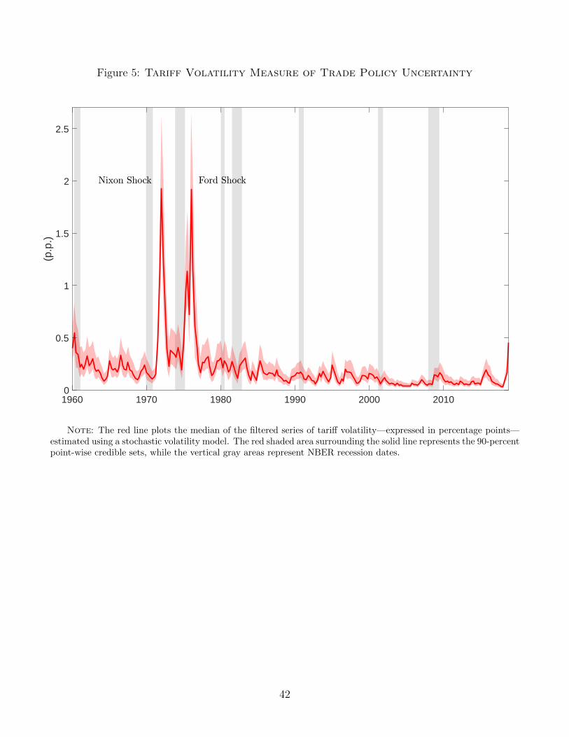
Figure 5: Tariff Volatility Measure of Trade Policy Uncertainty
1960 1970 1980 1990 2000 20100
0.5
1
1.5
2
2.5
(p.p
.)
Note: The red line plots the median of the filtered series of tariff volatility—expressed in percentage points—estimated using a stochastic volatility model. The red shaded area surrounding the solid line represents the 90-percentpoint-wise credible sets, while the vertical gray areas represent NBER recession dates.
42

Figure 6: Response of Capital to Firm-Level TPU-4
-3-2
-10
Perc
ent r
espo
nse
with
68%
c.i.
0 1 2 3 4Quarters
Note: Firm-Level response of investment at different horizons following an increase in firm-level TPU from 0 to0.035, its average value when TPU is greater than 0. The shaded areas denote 1 standard error confidence interval.Standard errors are two-way clustered by firm and quarter.
43

Figure 7: Response of Capital to Firm-Level TPU: Additional Analysis-4
-3-2
-10
Perc
ent r
espo
nse
with
68%
c.i.
0 1 2 3 4Quarters
1. Without Controls
-3-2
-10
1Pe
rcen
t res
pons
e w
ith 6
8% c
.i.
0 1 2 3 4Quarters
2. Trade Policy without Uncertainty
-3-2
-10
1Pe
rcen
t res
pons
e w
ith 6
8% c
.i.
0 1 2 3 4Quarters
3. No Time Effects
Note: Robustness. The thin red line is the response in the baseline experiment of Figure 6. Shaded areas denote1 s.e. confidence interval. Standard errors are two-way clustered by firm and quarter.
44

Figure 8: Investment and Industry TPU in 2018
Aircraft
Almost NothingApparel
Automobiles and Trucks
Beer & Liquor
Business Services
Business Supplies
Candy & Soda
Chemicals
Coal
Communication
Computer Hardware
Computer Software
Construction
Construction Materials
Consumer Goods
Defense Electrical Equipment
Electronic Equipment
Entertainment
Fabricated ProductsFood Products
Healthcare
Insurance
Machinery
Measuring and Control Equipment
Medical Equipment
Non-Metallic and Industrial Metal Mining
Personal Services
Petroleum and Natural Gas
Pharmaceutical Products
Precious Metals
Printing and Publishing
Real Estate
Recreation
Restaraunts, Hotels, Motels
Retail Rubber and Plastic Products
Shipbuilding, Railroad Equipment
Shipping Containers
Steel Works Etc
Textiles
Tobacco Products
Trading
TransportationWholesale
-10
-50
510
15C
apita
l Gro
wth
(Ppt
diff
eren
ce, 2
018
vs 2
017)
-1 0 1 2 3 4TPU (Change, 2018 vs 2017)
Note: Change in TPU in 2018 and change in investment in 2018 across industries.
45

Figure 9: The Investment Effects of TPU and Tariff Volatility Shocks
0 4 8 12Quarters
0
15
30
45
(%)
News-Based TPU Index
0 4 8 12Quarters
-2
-1
0
1
2
(%)
Private Investment
(a) Bivariate VAR with News-Based TPU
0 4 8 12Quarters
0
20
40
60
80
(%)
Tariff Volatility
0 4 8 12Quarters
-2
-1
0
1
2
(%)
Private Investment
(b) Bivariate VAR with Tariff Volatility
0 4 8 12Quarters
0
15
30
45
(%)
News-Based TPU Index
0 4 8 12Quarters
-2
-1
0
1
2
(%)
Private Investment
(c) Multivariate VAR with News-Based TPU
Note: The solid lines depict median responses of trade uncertainty indicators and private investment to a tradepolicy uncertainty shock of size two standard deviations. The VAR model is estimated on quarterly data from 1960to 2018. The shaded bands represent the 70-percent point-wise credible sets.
46

Figure 10: Impulse Responses to News and Uncertainty Shocks.
5 10 15 20
-1.5
-1
-0.5
0
%
from
SS
Investment
5 10 15 20-0.8
-0.6
-0.4
-0.2
0
%
from
SS
Consumption
5 10 15 20
-0.8
-0.6
-0.4
-0.2
0
%
from
SS
GDP
5 10 15 20
-300
-200
-100
0
100
from
SS
bpt
s a.
r.
CPI Inflation
5 10 15 20
-60
-40
-20
0
20
from
SS
bpt
s a.
r.
Interest Rate
5 10 15 20
-0.8
-0.6
-0.4
-0.2
0
0.2
0.4
%
from
SS
Price of Capital
5 10 15 20
-0.3
-0.2
-0.1
0
%
from
SS
Marginal Cost
5 10 15 20
-0.2
-0.1
0
0.1
pct
from
SS
Capital Differential
5 10 15 20
-1.5
-1
-0.5
0
pct
from
SS
Mass of Exporters
5 10 15 20-0.1
-0.05
0
0.05
0.1
pct
from
SS
Probability of Entry
5 10 15 20
-2
-1
0
pct
from
SS
Probability of Stay Exporter
News and UncertaintyNewsUncertainty
Note: Model Impulse Responses to News Shocks and Uncertainty Shocks. The horizontal axis measures quarterssince the shock.
47
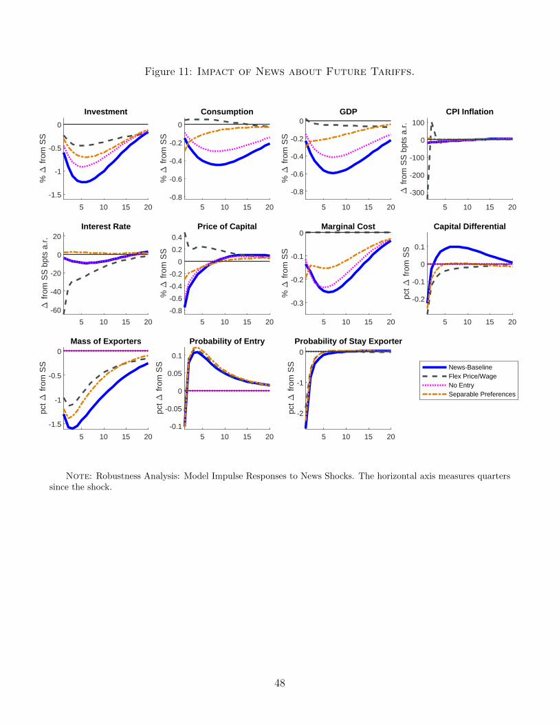
Figure 11: Impact of News about Future Tariffs.
5 10 15 20
-1.5
-1
-0.5
0
%
from
SS
Investment
5 10 15 20-0.8
-0.6
-0.4
-0.2
0
%
from
SS
Consumption
5 10 15 20
-0.8
-0.6
-0.4
-0.2
0
%
from
SS
GDP
5 10 15 20
-300
-200
-100
0
100
from
SS
bpt
s a.
r.
CPI Inflation
5 10 15 20
-60
-40
-20
0
20
from
SS
bpt
s a.
r.
Interest Rate
5 10 15 20
-0.8
-0.6
-0.4
-0.2
0
0.2
0.4
%
from
SS
Price of Capital
5 10 15 20
-0.3
-0.2
-0.1
0
%
from
SS
Marginal Cost
5 10 15 20
-0.2
-0.1
0
0.1
pct
from
SS
Capital Differential
5 10 15 20
-1.5
-1
-0.5
0
pct
from
SS
Mass of Exporters
5 10 15 20-0.1
-0.05
0
0.05
0.1
pct
from
SS
Probability of Entry
5 10 15 20
-2
-1
0
pct
from
SS
Probability of Stay Exporter
News-BaselineFlex Price/WageNo EntrySeparable Preferences
Note: Robustness Analysis: Model Impulse Responses to News Shocks. The horizontal axis measures quarterssince the shock.
48

Figure 12: Impact of Higher Uncertainty about Future Tariffs.
5 10 15 20
-1.5
-1
-0.5
0
%
from
SS
Investment
5 10 15 20-0.8
-0.6
-0.4
-0.2
0
%
from
SS
Consumption
5 10 15 20
-0.8
-0.6
-0.4
-0.2
0
%
from
SS
GDP
5 10 15 20
-300
-200
-100
0
100
from
SS
bpt
s a.
r.
CPI Inflation
5 10 15 20
-60
-40
-20
0
20
from
SS
bpt
s a.
r.
Interest Rate
5 10 15 20
-0.8
-0.6
-0.4
-0.2
0
0.2
0.4
%
from
SS
Price of Capital
5 10 15 20
-0.3
-0.2
-0.1
0
%
from
SS
Marginal Cost
5 10 15 20
-0.2
-0.1
0
0.1
pct
from
SS
Capital Differential
5 10 15 20
-1.5
-1
-0.5
0
pct
from
SS
Mass of Exporters
5 10 15 20-0.1
-0.05
0
0.05
0.1
pct
from
SS
Probability of Entry
5 10 15 20
-2
-1
0
pct
from
SS
Probability of Stay Exporter
Uncertainty-BaselineFlex Price/WageNo EntrySeparable PreferencesLow Price/Wage MarkupsLow Ale-Choi Markups
Note: Robustness Analysis: Model Impulse Responses to Uncertainty Shocks. The horizontal axis measuresquarters since the shock.
49

Appendix
A.1 Description of Firm-Level and Industry Data
Our firm-level data source is the Compustat North America database. Our key variables are invest-ment, cash flows, and Tobin’s Q, which we construct following standard approaches to Compustatdata in the literature (e.g. Ottonello and Winberry (2018)). Compustat variables names are shownin all capital letters.
1. Data preparation. We consider only firms with headquarters located in the United States(Compustat variable LOC is “USA”). We next drop observations with non-positive quarterlycapital expenditures (CAPXY), total assets (ATQ) less than $1 million in chained 2009 dollars,and acquisitions (AQCY) are greater than 5% of assets. Lastly we drop observations wherenet property, plant, and equipment (PPENTQ) decreases and then increases (or vice versa)more than fifty percent between two successive quarters.
2. Industries included. We exclude firms in the utilities, banking, and finance sectors (firms witha 4-digit Standard Industrial Classification (SIC) code in the ranges 4900-4999 and 6000-6299).We also restrict the sample to sectors trading in agricultural, mining, and manufacturing goods(3-digit NAICS codes in the ranges 111-115, 211-212, and 311-339), omitting wholesale andservice industries. These sectors are those for which we have complete data to construct ourmeasure of openness, but they are also those with higher instances of TPU Our final industryselection includes roughly half the original sample Compustat firms.
3. Investment. For our measure of investment log ki,t+h − log ki,t−1 (with h ≥ 0) we define afirm’s capital stock ki,t as gross property, plant, and equipment (PPEGTQ) in the first periodfor which there is data are available. Thereafter we use PPENTQ.
4. Tobin’s Q. We define Tobin’s Q as the ratio of a firm’s total market value to its total assetvalue, where market value is the book value of assets plus the market value of stock (priceat close (PRCCQ) * common shares CSHQQ)) less the book value of stock (CEQ). The final
measure is thus equal to ATQ+(PRCCQ∗CSHOQ)−CEQQATQ
. We winsorize the variable at the 1st and99th percentile.
5. Cash flows. We measure cash flows using the ratio of cash and short-term investments (CHEQ)to beginning-of-period property, plant, and equipment, which is the first lag of PPENTQ inour sample. We winsorize the variable at the 1st and 99th percentile.
6. Openness. Openness is defined at the 3-digit level of the North American Industry Classifi-cation System (NAICS). We use a standard measure equal to the ratio of an industry’s grossoutput to usage, where usage is gross output plus imports less exports. Using gross outputby industry from the Bureau of Economic Analysis’ Industry Economic Accounts Data andexports/imports by industry from the U.S. Census Bureau’s U.S. International Trade andGoods and Services report (FT900).
A.1

A.2 Stochastic Volatility Model: Robustness
In our bechmark empirical specification, we posit that tariffs follow an autoregressive process with(auturegressive) stochastic volatility. Table 1A compares our benchmark estimates to those obtainedfrom two alternative models. Model 1 includes feedback from lagged values of detrended outputand U.S. federal public debt. This approach follows closely the fiscal volatility rule adopted inFernandez-Villaverde et al. (2015) and is meant to capture the idea that the state of the businesscycle and the level of debt may influence behavior of government instruments, including tariffs.Model 2 allows for feedback from lagged values of detrended output and the U.S. net foreign assetposition. This rule incorporates the idea that developments in the external position of the UnitedStates, approximated by the net foreign asset position, may also affect the setting of tariffs.
Table 1A. Tariff Rule: Robustness
Benchmark Model 1 Model 2
ρτ0.99
[0.99; 0.99]0.99
[0.99; 0.99]0.98
[0.97; 0.99]
σ−6.14
[−6.73;−5.47]−6.35
[−6.84;−5.76]−6.05
[−6.32;−5.78]
ρσ0.96
[0.87; 0.99]0.93
[0.85; 0.97]0.85
[0.72; 0.92]
η0.37
[0.29; 0.47]0.39
[0.32; 0.49]0.37
[0.29; 0.47]
Note. Estimates refer to posterior medians. Numbers in brackets are the 90
percent probability interval.
Overall, we find that the inclusion of macroeconomic feedbacks does not greatly affect theestimation of the tariff rule parameters. The average standard deviation of tariffs varies from100*exp(-6.14) = 0.24 percentage point in the bechmark model to 0.18 (Model 1) and 0.24 (Model2). Model 2 also seems to have a slightly lower volatility persistence than our benchmark model(0.85 vs 0.96). A one-standard deviation shock to tariff volatility increases the volatility by about10 basis points in all models.
A.2

A.3 Additional Tables
Table A.1: Episodes of High Aggregate Trade Policy Uncertainty
U.S. Administration Policy Action Quarter Quotes or Additional Narrative Material
President Kennedy Trade Negotia-tions
1960q1 ”This is the year to decide. The Reciprocal Trade Act is expiring. We need a new law—awholly new approach—a bold new instrument of American trade policy. Our decisioncould well affect the economic growth of our Nation for a generation to come. ”
President Nixon Tariff Increase 1971q4 ”I am taking one further step to protect the dollar, to improve our balance of payments,and to increase jobs for Americans. As a temporary measure, I am today imposing anadditional tax of 10 percent on goods imported into the United States. This is a bettersolution for international trade than direct controls on the amount of imports. Thisimport tax is a temporary action...When the unfair treatment is ended, the import taxwill end as well.”
President Ford Tariff Increase 1975q2 ”...we need immediate action to cut imports. ...Therefore, I am using Presidential powersto raise the fee on all imported crude oil and petroleum products...To that end, I am re-questing the Congress to act within 90 days on a more comprehensive energy tax program.It includes: excise taxes and import fees totaling $2 per barrel on product imports and onall crude oil; deregulation of new natural gas and enactment of a natural gas excise tax...Iam prepared to use Presidential authority to limit imports, as necessary, to guaranteesuccess...To provide the critical stability for our domestic energy production in the face ofworld price uncertainty, I will request legislation to authorize and require tariffs, importquotas, or price floors to protect our energy prices at levels which will achieve energyindependence.”
Note: Narrative analysis of major increases in aggregate trade policy uncertainty.
A.3

Table A.2: Selected Quotes from Earnings Call Transcripts Mentioning Trade Policy Uncertainty
Company Name Sector Quarter ∆K+1 TPU Selected Quotes Mentioning Trade Policy Uncertainty
SUNPOWER ElectronicEquipment
2017q3 -14.6 2 In September, the ITC is scheduled to decide whether to recommend the imposition ofimport tariffs or quotas on solar panels and to subsequently propose specific remediesin November. [...] the requested remedies could significantly impact the U.S. solarmarket, imposing a direct burden on manufacturers
BUILDERSFIRSTSOURCE
ConstructionMaterials
2017q2 -11.0 3 Q: [...] on the lumber import tariff how have you handled [...] the tariff and the pricevolatility? [...] A: Yes, could be a slight headwind to working capital.
RENEWABLEENERGY GROUP
Petroleum andNatural Gas
2017q3 -9.5 2 Q: I wanted to ask thoughts around the postponed EU vote last week around Ar-gentina’s challenge to the EU antidumping duties there and if there is the potential forgallons to potentially flow back into the EU from Argentina and Indonesia. A: Well,we were certainly watching that as it affects our European operation margins...
WEYERHAEUSER ConstructionMaterials
2017q3 -5.7 2 On June 26, the Department of Commerce announced preliminary antidumping dutieson Canadian lumber producers. For most producers, the duty will be approximately 7percent and will also be assessed retroactively. [...] The government will continue itsinvestigation through the remainder of the year, as the Department of Commerce andInternational Trade Commission collect and evaluate additional information in supportof final determinations of the duties and a level of material injury to U.S. producers.These determinations are expected later this year. The U.S. coalition continues to workclosely with the Department of Commerce, and we remain hopeful we will be able toreach a quota-based agreement.
RENEWABLEENERGY GROUP
Petroleum andNatural Gas
2017q4 -6.2 2 Finally, antidumping determinations are expected in early January. Based on thesevery positive preliminary rulings, we are confident that the final decision will be sup-portive of domestic biodiesel production.
BROADWINDENERGY
Machinery 2017q3 -3.1 3 Q. Have you done any type of quantitative impact or assessment on [...] the towersbusiness, but potentially all of your segments, if such a [steel] tariff was put into place?A. It’s not – would not be a good thing, because of the steel that we consume in ourbusinesses.
RENEWABLEENERGY GROUP
Petroleum andNatural Gas
2017q2 -5.4 2 [...] Our industry trade group took on an initiative to pull domestic producers togetherin a coalition to just ask for a fair trade, a level playing field and countervailing dutiesand antidumping against 2 countries.
MOHAWKINDUSTRIES
Textiles 2017q2 -2.9 2 Q. Great. Any potential impact from the proposed Canadian tariff? A. Listen, if youcan tell me what the proposals will look like, I’ll decide what it is.
CABOT CORP Chemicals 2016q2 -2.3 2 There is some concern about [inventories] – with anti-dumping duties against trucktires out of China that, that could cause the same phenomenon to happen again. ButI think we are probably closer to natural inventory levels than certainly we were overthe last 18 months or so as those passenger car duties were implemented.
INTL PAPER Business Supplies 2015q2 -2.1 2 Q. ... Just turning to Brazil. [...] Potentially, higher taxes and tariffs on energy usage.A. I mean, the Brazil packaging business is in the same market, experiencing the samedynamics as our paper business. So, demand has been a challenge.
FORD MOTOR Automobiles andTrucks
2017q1 -.8 2 Q. You clearly mentioned the prospects of an import tariff. There is [...] probability of aborder tax adjustment, and if that doesn’t happen, then we’re just going to see importtariffs. A. [...] whether it’s a border tax or border adjustment, as Bob mentioned, thisis a multifaceted blueprint that’s out there.
Note: Selected mentions of firm-level trade policy uncertainty extracted from the earnings call which are followedby a decline in firm-level investment in the next calendar quarter. The ∆K column indicates the percent change inthe firm’s capital stock in the calendar quarter subsequent to the mention. The TPU column lists the total numberof mentions of trade policy uncertainty in the transcript of the earnings call.
A.4

A.4 Additional Figures
Figure A.1: Comparison with Hassan et al. (2017)
810
1214
16Ag
greg
ate
TPU
from
Has
san
et a
l.
0.0
5.1
.15
Earn
ings
Cal
ls: A
ggre
gate
TPU
2005q1 2010q1 2015q1 2020q1Calendar Quarter
Earnings Calls: Aggregate TPU Aggregate TPU from Hassan et al.
Note: Aggregate TPU from earnings calls in this paper and in Hassan et al. (2017)
Figure A.2: Comparison with Baker, Bloom, and Davis (2016)
050
100
150
200
250
015
030
045
060
075
0
1960 1980 2000 2020
CIMPR TPU (right axis) BBD TPU (left axis)
TPU: Caldara et al. (2019) vs. Baker et al. (2016)
Note: News-based TPU in this paper and in Baker, Bloom, and Davis (2016).
A.5