IZA DP No. 3619

The Economic Growth Impact of Hurricanes:Evidence from US Coastal Counties

Eric Strobl

DI

SC

US

SI

ON

PA

PE

R S

ER

IE

S

Forschungsinstitutzur Zukunft der ArbeitInstitute for the Studyof Labor

July 2008

The Economic Growth Impact of

Hurricanes: Evidence from US Coastal Counties

Eric Strobl Ecole Polytechnique Paris

and IZA

Discussion Paper No. 3619 July 2008

IZA

P.O. Box 7240 53072 Bonn

Germany

Phone: +49-228-3894-0 Fax: +49-228-3894-180

E-mail: iza@iza.org

Any opinions expressed here are those of the author(s) and not those of IZA. Research published in this series may include views on policy, but the institute itself takes no institutional policy positions. The Institute for the Study of Labor (IZA) in Bonn is a local and virtual international research center and a place of communication between science, politics and business. IZA is an independent nonprofit organization supported by Deutsche Post World Net. The center is associated with the University of Bonn and offers a stimulating research environment through its international network, workshops and conferences, data service, project support, research visits and doctoral program. IZA engages in (i) original and internationally competitive research in all fields of labor economics, (ii) development of policy concepts, and (iii) dissemination of research results and concepts to the interested public. IZA Discussion Papers often represent preliminary work and are circulated to encourage discussion. Citation of such a paper should account for its provisional character. A revised version may be available directly from the author.

IZA Discussion Paper No. 3619 July 2008

ABSTRACT

The Economic Growth Impact of Hurricanes: Evidence from US Coastal Counties*

We estimate the impact of hurricane strikes on local economic growth rates and how this is reflected in more aggregate growth patterns. To this end we assemble a panel data set of US coastal counties’ growth rates and construct a hurricane destruction index that is based on a monetary loss equation, local wind speed estimates derived from a physical wind field model, and local exposure characteristics. Our econometric results suggest that in response to a hurricane strike a county’s annual economic growth rate will initially fall by 0.8, but then partially recover by 0.2 percentage points. While the pattern is qualitatively similar at the state level, the net effect over the long term is negligible. Hurricane strikes do not appear to be economically important enough to be reflected in national economic growth rates. JEL Classification: E0 Keywords: hurricanes, economic growth, US coastal counties Corresponding author: Eric Strobl Department of Economics Ecole Polytechnique 91128 Palaiseau Cedex France E-mail: eric.strobl@polytechnique.edu

* I am grateful for financing from La Chaire Développement Durable of the Ecole Polytechnique.

2

1. Introduction

Given the potential havoc and destruction caused by hurricanes, the common

fascination with these generally unpredictable events is not surprising. For instance, the

unfolding destruction of Hurricane Katrina in 2005, estimated by Pielke et al (2008) to have

caused over 80 US billion dollars in damages in Lousiana and Missippi alone, was followed on

television by millions worldwide. Worryingly in this regard is that there appears to be an

increasing trend in the number and strength of hurricanes over the last decade1, which some

argue is linked to global warming.2 Moreover, the regions directly affected, i.e., coastal areas,

are, at least in the US, those where a large and growing part of total economic activity is located

and hence the regions that are also driving a substantial portion of national economic growth.3

Thus, accurately assessing how economies are likely to be affected by striking hurricanes, both

at the local and at the national level, is arguably of considerable importance to policymakers

and academics alike.

The primary negative impact of hurricanes on affected regions involves the (permanent)

destruction of property in terms of housing, capital stock, and agricultural crops, where losses

in these factors may additionally lead to a (temporary) disruption in production in many

industries.4 However, at the same time the subsequent receipt of disaster assistance, clean-up

and recovery activity, and the production of replacement capital will serve to act as a

counterweight to any losses.5 Additionally some of the losses may be insured and payments in

this regard may be coming from outside the affected region. Uncertainty regarding the exact

1 Webster et al (2005).

2 See, for example, Emanuel (2005), Nordhaus (2006), and Elsner (2007).

3 Rappaport and Sachs (2003).

4 Although there may be some losses in life, these tend nowadays at least in the US to be negligible.

5 See Horwich (2000) for a discussion of this.

3

interplay and relative size of these factors means that the net economic effect of hurricane

strikes is not at all obvious. Moreover, even if the losses largely outweigh the boosts to local

economic growth from recovery activity, it is not clear to what extent this may be reflected in

more aggregate growth patterns, since hurricanes, as most natural disasters, tend to be very

localized phenomina relevant only for particular regions.6

Surprisingly, however, as of date there is to the best of our knowledge no

comprehensive study, for the US or elsewhere, of how hurricane strikes may have affected local

growth patterns and how any local impact translates into more aggregate levels of economic

growth.7 More precisely, while there are a few papers that have examined the local impact of

hurricanes, these have either focused on particular types of micro-level responses or dealt with

the impact on the local labour market. For instance, Evans et al (2008) discover that fertility

rates in the US Atlantic and Gulf of Mexico region change in response to hurricanes. Also,

Belasen and Polacheck (2008) show that employment in Florida employment fell in response to

hurricanes by between 1.5 and 5 per cent. From a macro-economic perspective there are, in

contrast, a handful of papers that provide estimates of the growth impact of hurricane strikes.

For instance, Bluedorn (2005) studies the response of the current account to hurricane activity

in the Central American and Caribbean region and his findings suggest that the median

damaging hurricane will cause output to fall by 0.3 percentage points, while Strobl’s (2008)

study of the same region suggests that economic growth rates are reduced by 0.8 percentage

6 As a matter of fact, in a study of the Kobe earthquake in Japan, which was the most severe earthquake in modern

times to strike an urban area, Horwich (2005) looking at GDP patterns over the period argues that there were no

observable macroeconomic effects. 7 One may want to note, for instance, that even in the US there is no official systematic data collection on the

impact of natural disasters and that while standard source data for GDP and income incorporate the effect they do

not separately identify it. See http://www.bea.gov/katrina/index2.htm.

4

points for an average destructive hurricane. However, it is not clear whether such results from

developing county samples are very relevant for a industrialized economy like the US, given

that it appears to be a stylized fact in the literature that economic losses due to natural

disasters are negatively correlated with economic wealth.8

In this paper we thus explicitly set out to estimate the net growth impact of hurricanes

on affected local economies, as well as to what extent such effects spill over into more

aggregate economic growth patterns. To this end we develop a hurricane destruction index

that is based on a monetary loss equation, local wind speed estimates derived from a physical

wind field model, and local exposure characteristics and estimate its impact on the growth

rates of a panel of counties in the relevant US coastal area. Our econometric results suggest

that in response to a hurricane strike a county’s annual economic growth rate will initially fall

by 0.8, but then partially recover by 0.2 percentage points. This is arguably a relative large

impact given that the average annual county level growth rate is around 1.68 per cent. While

the pattern is qualitatively similar at the state level, the overall the net long term effect is

negligible. Hurricane strikes do not appear to be economically important enough to be

reflected in national economic growth rates.

The remainder of the paper is organized as follows. In the following section we describe

the nature of hurricanes and their destruction potential. Section III introduces our hurricane

destruction proxy. In Section IV we describe our data. The econometric analysis is contained in

Section V. Finally, concluding remarks are given in the final section.

8 See, for instance, Kahn (2005) and Toya and Skidmore (2007).

5

2. Some Basic Facts about Hurricanes and their Destructive Power

A tropical cyclone is a meteorological term for a storm system, characterized by a low

pressure system center and thunderstorms that produce strong wind and flooding rain, which

generally first forms, and hence its name, in tropical regions of the globe.9 Depending on their

location and strength, tropical cyclones are referred to by various other names, such as

hurricane, typhoon, tropical storm, cyclonic storm, and tropical depression. Tropical storms in

the North Atlantic Basin, as we study here, are termed hurricanes if they are of sufficient

strength.10 Their season can start as early as the end of May and last until the end of

November, although it generally takes place between July and October.

We depict a radar composite picture of Hurricane Andrew, which made landfall in

Florida on August 24 in 1992, as a typical example of a hurricane in Figure 1. As can be seen, in

terms of its structure, a hurricane will generally harbor an area of sinking air at the center of

circulation, known as the ‘eye, where weather in the eye is normally calm and free of clouds,

though, if over the ocean, the sea under the eye may be extremely violent.11 Outside of the eye

curved bands of clouds and thunderstorms move away from the eye wall in a spiral fashion,

where these bands are capable of producing heavy bursts of rain, wind, and tornadoes. One

may want to take note that a hurricane appears to affect a large area surrounding its eye and

that its structure is not symmetric. As a matter of fact, hurricane strength tropical cyclones are

generally about 500 km wide, although they can vary considerably. Hurricanes are for

9 The term "cyclone" derives from the cyclonic nature of such storms, with counterclockwise rotation in the

Northern Hemisphere and clockwise rotation in the Southern Hemisphere. 10

Generally at least 119 km/hr. In order to be considered a tropical storm the storm must have maximum wind

speed of at least 55 km/hr. To be upgraded to a hurricane these speeds must reach at least 119 km/hr. 11

National Weather Service (October 19, 2005). Tropical Cyclone Structure. JetStream - An Online School for

Weather. National Oceanic & Atmospheric Administration.

6

convenience sake typically categorized in terms of their wind speed on the Saffir-Simpson Scale,

where the scale ranges from 1 to 512, although Category 5 hurricanes are fairly rare in the North

Atlantic Basin.13 One may also want to note that hurricanes generally lose their strength

quickly as they move over land due to land friction and the lack of moisture and heat that the

ocean would provide.14

Physical damages due to hurricanes typically take a number of forms. Firstly, the strong

winds associated with the storm may cause considerable structural damage to buildings as well

as crops. Secondly, there is generally strong rainfall associated with a hurricane, which can

result in extensive flooding and, in sloped areas, landslides. Finally, the high winds pushing on

the ocean’s surface can cause the water near the coast to pile up higher than the ordinary sea

level, and this effect combined with the low pressure at the center of the weather system and

the bathymetry of the body of water results in storm surges. Generally these surges are the

most damaging aspect of hurricanes. In particular, storm surges can cause severe property

damage, as well as destruction and salt contamination of agricultural areas.15 Such flooding

may extend up to 40km or more from the coast for maximum strength storms.

3. A Hurricane Destruction Proxy

Previous studies of the local impact of hurricane destruction have resorted to using

simple measures of hurricane incidence or their maximum observed Saffir-Simpson scale

category as the hurricane eye passes directly over locations as a proxy of their local

12

Scale definitions in terms of miles per hour: (1) 119-153, (2) 154-177, (3) 178-209, (4) 210-249, and (5) 250+; 13

Willoughby and Black (1995). 14

See NOAA at http://www.aoml.noaa.gov/hrd/tcfaq/C2.html. 15

Yang (2007).

7

destruction.16 As outlined earlier, in reality hurricanes may have a destructive impact on

spatially potentially very large areas, and not just where the eye directly passes over.

Moreover, the extent of this destruction is unlikely to be uniform across localities, but will

depend on the position relative to the eye, the maximum wind speed, and local characteristics,

amongst other things.

In order to take account of the complex nature of hurricanes we thus here, in contrast

to the previous literature, avail of a proxy of local wind speed experienced that is derived from

a model of the spatial structure and movement of hurricanes, and hence of wind speeds

experienced directly along the track as well as locations around it. We then translate these

local wind speeds into a proxy of local destruction. More precisely, as noted by Emanuel

(2005), both the monetary losses in hurricanes as well as the power dissipation of these storms

tend to rise roughly to the cubic power of maximum observed wind speed.17 Consequently, he

proposes a simplified power dissipation index that can serve to measure the potential

destructiveness of hurricanes as18:

PDI = ∫τ

0

3dtV (1)

where V is the maximum sustained wind speed, and τ is the lifetime of the storm as

accumulated over time intervals t. Here we modify this index to obtain a proxy of damages due

16

See, for instance, Belasen and Polacheck (2007). 17

18 This index is a simplified version of the power dissipation equation rddtVCPD

r

D

t 3

00

0

2 ∫∫= ρπ where the

surface drag (CD), surface air density (ρ), and the radius of the storm (r0) are taken as given since these are

generally not provided in historical track data. Emanuel (2005) notes that assuming a fixed radius of a storm is

likely to introduce only random errors in the estimation. He similarly argues that surface air density varies over

roughly 15%, while the surface drag coefficient levels off at wind speeds in excess of 30m/s, so that assuming that

their values are fixed is not unreasonable.

8

to hurricanes at the county level i using census tract level j data. More precisely, the total

destruction due to the r=1,…k storms that affected county i at time t is assumed to be :

HURRi,t = ∑∑= =

m

j

k

r

tjitrji wV1 1

,,,,,

3

(2)

where V is an estimate of the wind speed due to storm r observed in census tract j at time t, to

be described in detail in Section III. The w’s are weights assigned according to characteristics of

the affected census tracks intended to capture geographical differences within counties in

terms of the potential exposure if a hurricane were to strike. In this regard, we use the time

varying share of population of each individual census tract in its county at t-1, where the

underlying argument is that of two equally affected (in terms of wind speed) areas the one

where more people live is likely to be more important in terms of adding to county level

damage incurred.19

Finally, one should note that Nordhaus (2006) argues that the relationship of costs and

wind speed is in fact not to the cubic, found by Emanuel (2005), but rather to the eighth

power. More specifically, he regresses the log of the cost per hurricane normalized by US GDP

on the logged maximum wind speed for a set of 20th century hurricanes and finds a coefficient

of 7.6 on the wind speed. However, further investigation using his data demonstrates that this

result is sensitive to the measure of cost he uses. In particular, arguably US GDP is unlikely to

be a good normalization for costs, since hurricanes typically only affect areas close to the coast

and not all of the US. Moreover, the relative local wealth that was affected is likely to have

19

While when first delineated census tracts are designed to be homogeneous with respect to population

characteristics, economic status, and living conditions, population size tends to change over time, particularly for

coastal counties. The census tracts’ population size in our sample of coastal counties varies between around 2,500

and 8,000 inhabitants.

9

changed substantially over the period as coastal communities have grown in size and income.20

When one instead regresses the log of the normalized cost values calculated by Pielke et al

(2005) - who normalize damages with regard to changes in inflation, population, and wealth of

affected counties only - on the log of maximum observed wind speeds of the hurricanes in

Nordhaus’ data set, one finds that the resultant coefficient implies that costs rise instead to

about the 3.6th power of wind speed, and thus much more in line with Emmanuel (2005) and

supportive of the proxy that we use in (2).

3. Data

3.1 Geographic Area of Study

Normally only a small proportion of total geographic area of the US, namely that

relatively close to the coast, is affected by hurricanes since these quickly lose speed once they

become landfall. Moreover, as outlined earlier, storm surges generally cause most of the

damages due to hurricanes, and this again is most relevant for coastal areas. We thus

specifically focus our analysis on the US coastal counties in the North Atlantic Basin region. In

terms of identifying coastal counties in this region we rely on the list generated by the Strategic

Environmental Assessments Division of the National Oceanic and Atmospheric Administration

(NOAA). Accordingly, coastal counties are defined as those which have at least 15 per cent of

their land in the coastal watershed21 or that comprise at least 15 per cent of a coastal

20

See Rappaport and Sachs (2003). 21

A coastal watershed is composed of all lands within Esturaine Drainage Areas (EDA) or Coastal Drainage Areas

(CDA) in the NOAA’s Coastal Assessment Framework.

10

cataloging unit22. Within the hurricane relevant North Atlantic Basin region this constitutes a

total of 409 coastal counties located over 19 states. We show these, in grey colour, in Figure 2.

3.2 Economic Growth Data

To construct proxies of county level per capita economic growth rates and per capita

wealth we resort to the Bureau of Economic Analysis’(BEA) Local Area Personal per Capita

Income county level estimates available since 1969. Personal income in the BEA data is defined

as the income received by all persons from all sources and constitutes the sum of net earnings

by place of residence, rental income of persons, personal dividend income, personal interest

income, and personal current transfer receipts. We convert these nominal values to constant

2005 dollars using the US consumer price index. As can be seen from the summary statistics in

Table 1, the average annual county growth rate over the 1975 to 2005 period was 1.68.

However, the high standard deviation relative to this mean indicates that it varies substantially

over time and across space within our coastal community sample.

One should note that the BEA specifically discusses how natural disasters are likely to be

accounted for in their personal income estimates.23 In particular they argue that natural

disasters generally will have two major effects on the data. Firstly, there will be destruction of

property, where property losses net of the associated insurance claims will be incorporated as

one-time effects.24 In this regard, damage to property of household enterprises will reduce

proprietors’ income and rental income by the amount of uninsured losses, measured by

consumption of fixed capital less of business transfers. Damage to consumer goods, on the

22

A coastal cataloging unit is a drainage basin that falls entirely within or straddles an EDA or CDA. 23

http://www.bea.gov/katrina/index2.htm 24

For example, the BEA estimated that Hurricanes Katrina, Rita, and Wilma reduced nonfarm proprietors’ income

and rental income of persons net of business current transfer payments in Louisiana by 18,243 millions of dollars in

2005.

11

other hand, will affect personal current transfer receipts net of the amount of insured losses of

these goods. The second effect of natural disasters is likely to be a disruption of the flow of

income in the economy as normal economic activity is interrupted. This will generally be

embedded within the data on which the personal income estimates are based. For example,

many industries in the directly affected area will experience a reduction in earnings as

production is interrupted, while for others there may be an increase. Typically, however, these

income flows are reduced in the short-term (e.g., a reduction in consumer spending) and are

boosted later (e.g., an increase in construction activity).

3.3 Population Data

In order to make (2) operational we need data on both local wind speeds as well as

population shares. Our census tract level population shares, i.e., the w’s, are derived from the

decennial population census 1970, 1980, 1990, and 2000, where the calculated shares were

linearly interpolated to estimate annual values between these years for each census tract. As

can be seen from Table 1 the average census tract has nearly 5 per cent of total county level

population, albeit with considerable variation.

3.4 Hurricane Data

Since historical data on hurricanes normally only provide wind speeds at locations

where the eye passes over, one needs to simulate these for areas surrounding the eye. The use

of mathematical simulation methods to estimate local hurricane wind speeds was first

introduced by Russel (1968) and a large number of studies have since followed his proposed

methodology.25 The basic approach in all of these studies has essentially been to take site

25

See, for instance, Batts et al (1980), Georgiou (1985) and Vickery and Twisdale (1995).

12

specific statistics of key hurricane parameters, including the radius to maximum wind speed,

heading, translation speed, and the coast crossing position or distance to closest approach,

implement a Monte Carlo simulation to sample from each distribution, use a mathematical

representation of a hurricane along a straight path that satisfies the sampled path, and then

record the simulated wind speeds. Here we use wind speed data generated from a new wind

field model that is arguably superior to previous methods26, and now provides the underlying

data for hurricane loss modeling in the well known HAZUS software.27 In this model the full

track of a hurricane is modeled, beginning with its initiation over the ocean and ending with its

final dissipation. In essence it consists of two main components: (1) a mean flow wind model

that describes upper level winds and (2) a boundary layer model that allows one to estimate

wind speeds at the surface of the earth over a set of rectangular nested grids given the

estimated upper level wind speeds. The mean flow model underlying the HAZUS data is that

developed by Vickery et al (2000), which solves the full nonlinear equations of motion of a

translating hurricane then parameterizes these for use in simulations. One should note that

compared to previous approaches this allows for a more accurate characterization of

asymmetries in fast-moving hurricanes. The boundary layer model used is that of Vickery et al

(2008) which is based on a combination of velocity profiles computed using dropsond data and

a linear hurricane boundary layer model. Its advantage, compared to earlier methods, lies in

producing better estimates of the effect of the sea-land interface in reducing wind speeds and a

more realistic representation of the wind speeds near the surface and for better. Extensive

26

See FEMA (2007). 27

HAZUS is a GIS-based natural hazard loss estimation software package developed and freely distributed by

FEMA.

13

verification through comparison with real hurricane wind speed data showed that this new

wind speed model provided a good presentation of hurricane wind fields.28 In its most recent

release of HAZUS (version MR3), the above methodology was implemented to generate

maximum wind speeds, if these were at least 50 miles per hour, at the census tract level using

historical hurricane tracks of tropical storm that were at least of category 3 at the time of US

landfall over 1900 through 2005 as given in the HURDAT database.29, 30

We first depict all tropical storm activity in the North Atlantic Basin close to the US coast

over the 1970-2005 period as contained in the HURDAT database, even if these did not make

the HAZUS cut-off criteria, in Figure 3 – where the red portion of the lines indicates speeds of at

least hurricane strength. As can be seen, while many storms transverse the basin, only a small

portion make landfall on the US coast.

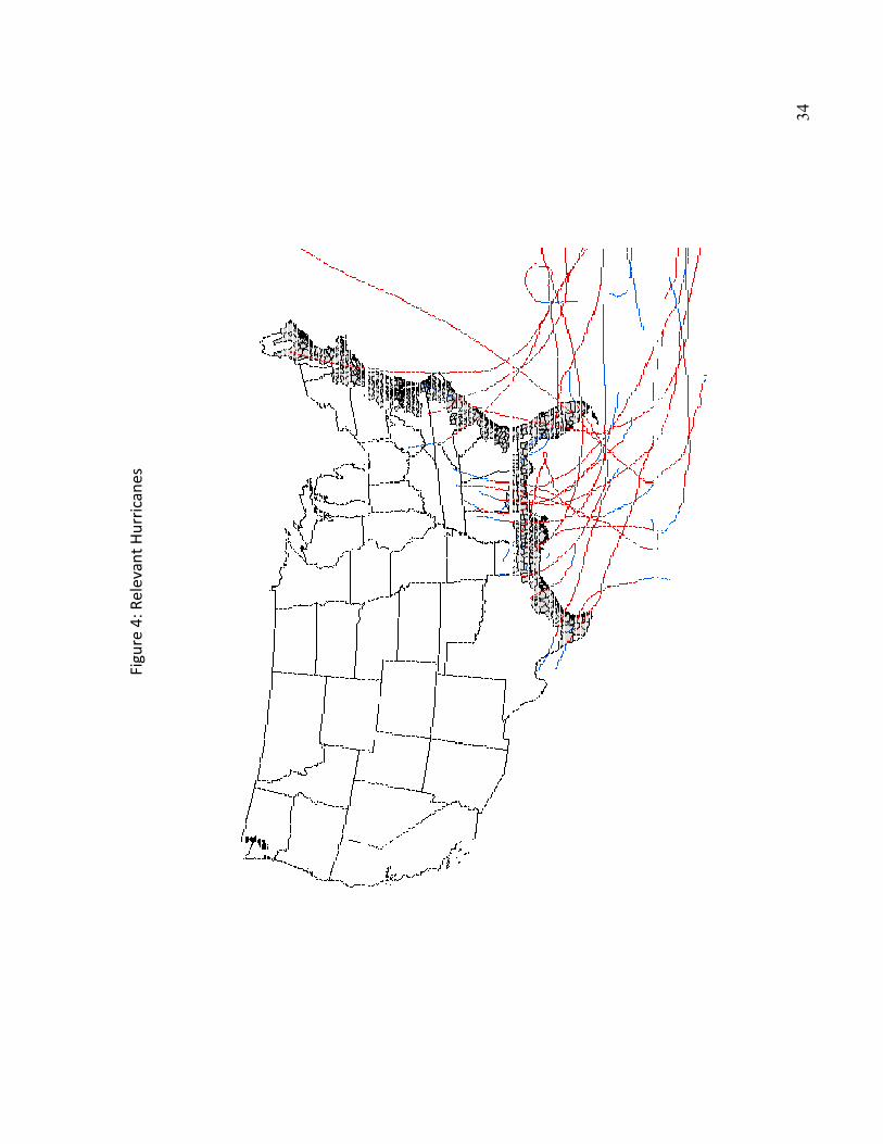
For our benchmark period, 1970-2005, 21 hurricanes in the HURDAT database made the

HAZUS cut-off criteria, and hence for which we have local wind field estimates, and we list

these in Table 2. We also depict their tracks in Figure 4 and two points are noteworthy in this

regard. Firstly, various counties along the whole coastline were affected, although especially in

Florida, Alabama, Mississippi, Louisiana, and Texas. Secondly, most hurricanes lose wind speeds

fairly quickly to be considered hurricanes or even tropical storms once they leave the coastal

area.

3.5 The Hurricane Destruction Proxy

28

FEMA (2007). 29

We would like to thank Frank Lavelle for provision of the data. 30

The HURDAT database consists of six-hourly positions and corresponding intensity estimates in terms of

maximum wind speed of tropical cyclones in the North Atlantic Basin over the period 1851-2006 and is the most

complete and reliable source of North Atlantic hurricanes; see Elsner and Jagger (2004).

14

To demonstrate the role of the individual components, i.e., V and w, in our hurricane

damage proxy, HURR, we resort again to the Hurricane Andrew example shown in Figure 1. It

first made landfall in Miami-Dade County in Florida on the 24th of August 1992 and then later

crossed into southwest Louisiana. One shold note that it is considered the second-most-

destructive hurricane in U.S. history31, and the last of three Category 5 hurricanes that made

U.S. landfall during the 20th century.32 Wind speeds during landfall reached over 115 miles per

hour and storm surges were as high as 5.2 meters in Southern Florida. In terms of damage,

Andrew caused around $26.5 billion worth ($38.1 billion in 2006 US dollars), with most of that

damage cost in south Florida.

Hurricane Andrew’s complete track as taken from HURDAT is shown in Figure 5, where

again the red portion of the line indicates when the storm was of hurricane intensity. As can be

seen, Andrew maintained hurricane strengths even as it made a second landfall in Louisiana,

but then was reclassified as a tropical storm once it left the state. The wind speeds generated

from the HAZUS wind field model for Florida by census tract along with the actual hurricane

tract (the dotted black line) are shown in Figure 6, where darker shading indicates stronger

wind speed. Accordingly, these correspond fairly well to what one would expect from the radar

composite image of the hurricane given in Figure 1. The highest wind speeds were experienced

along the track of the hurricane33, but even census tracts over 180km34 away from the actual

track of the hurricane eye were subject to potential damage through wind.

31

It was the most destructive hurricane until the arrival of Katrina in 2005. 32

Landsea et al (2004). 33

The highest wind speed was calculated to be in Dade county, measuring around 157 miles per hour. 34

For example, census tracts within Broward County at the time of landfall experienced up to 92 miles per hour.

15

In terms of assessing how the local exposure to potential damages may vary by census

tract with regard to its county level importance, i.e., the w’s, we depict the census tract level

population share (of a county) in Figure 7, where darker shading again indicates higher values.

One should in particular note that these weight components are not evenly distributed across

Southern Florida census tracts within counties. More specifically, it is clear that census tracts

on the west coast tend to have a greater share of a county’s population than those on the east.

This is in part of course due to fact that there are fewer census tracts within counties in the

former area.

The derived coastal values of HURR for Andrew using our proxies V and w in (2) are

depicted in Figure 8, where darker shading indicates higher values. Again it is obvious that

while most of the damage is found along the hurricane’s path, other counties both neighboring

and further away were also affected. More precisely, in Florida essentially all of the southern

tip was affected, while in Luisiana large parts of the state was subject to damaging wind speeds.

Additionally, a small part of Mississippi was affected when Andrew first entered the state.

Finally, we show the mean value of HURR for all coastal counties over the sample period

1970 to 2005. Accordingly, almost all counties were affected at least once since the 1970s.

Most destruction was, unsurprisingly given Figure 9, suffered in Florida, Alabama, Mississippi,

Louisiana, and Texas.

4. Econometric Estimation and Results

4.1 Econometric Specification

16

Our first econometric task is to investigate the economic growth impact of hurricane

strikes at the county level using our index of destruction. To do so we specify the following

simple conditional convergence growth equation: 35

GROWTHi,t-1→t = α + β1log(INITIALi,t-1) + β2HURRi,t + εi,t (3)

where GROWTH is the per capita economic growth rate in county i over t-1 to t, INTIAL is the

initial wealth per capita in county i at time t-1, HURR is our county level destruction proxy,

summed over all hurricanes r and all census tracts within counties i at time t, and ε is an error

term.

One should note that with the inclusion of the initial level of wealth per capita term one

could easily rewrite (3) to be a dynamic panel model with the lagged dependent variable as one

of the regressors. However, it is well known that in many cases dynamic panel regressions are

characterized by a systematic bias in the estimator of the coefficient on the lagged dependent

variable, as first identified by Nickell (1981). Furthermore, this potential bias in the

convergence term may lead to a bias in other coefficients in the model. Thus standard panel

estimator such as the Least Squares Dummy Variable (LSDV) or fixed effects would be

inappropriate. In order to correct for the bias we hence employ Bruno’s (2005) bias corrected

LSDV estimator36, which extends the original estimator by Kiviet (1995).37 Standard errors on

35

Noy (2007) uses a similar set-up investigating the macroeconomic consequences of natural disasters affect using

cross-country cost data from the EM-DAT database. 36

As initial estimates of the coefficients we use those produced by the Anderson and Hsiao (1982) estimator. 37

Another option would be to use the now standard GMM estimator, such as that proposed by Arellano and Bond

(1991), or some IV estimator such as Anderson and Hsiao (1982). However, as shown by Judson and Owen (1999),

the corrected LSDV estimator is more efficient and performs better in a panel where the number of individual units

is not particularly large and the time dimension not short, as we have here.

17

the coefficients are generated via bootstrapping methods, as suggested by Kiviet and Bun

(2001).38

One worry with (3) is that there may be spatial dependence between counties’ growth

rates that are geographically near. To address this with US county data Rappaport and Sachs

(2003) and Higgins et al (2006) use Conley’s (1999) correction to obtain standard errors that are

robust to such spatial correlation. Given that the econometric estimator we use necessitates

standard errors to be bootstrapped, we instead explicitly model the spatial dependence

between nearby counties’ growth rates by including a variable NGROWTHi,t-1→t capturing the

average per capita economic growth rate over t-1 to t in nearby coastal counties.39 More

precisely, we follow Higgens et al (2007) and assume that there is a cut-of distance of 200km,

after which two counties’ growth rates are independent of each other. To arrive at an average

value for those that fall within the cut-off distance we impose a declining weight structure g(dij)

= 1(dij/200), where dij is the distance between the centers of counties i and j. We then identify

all nearby counties surrounding county i that fall within this cut-off distance, multiply their

GROWTH values by g and take the mean of this product as NGROWTH.

4.2 Econometric Results

38

While Kiviet and Bun (2001) derive an analytical expression for the asymptotic vairance-covariance matrix of the

bias corrected LSDV estimator, Monte Carlo simulations suggested that it performed poorly, and hence the authors

suggest using a parametric boostrap estimator which takes account of the autoregressive nature of the data

generating process (DGP) by bootstrapping from each panel unit. We employ this boostrapping technique here

with our county level data. One worry in our context in this regard may also be spatial dependence of the DGP. As

a ‘rough’ way of taking account of this we experimented with bootstrapping from each state group of coastal

counties. This made, however, little difference to the estimated standard errors. 39

Higgins et al (2007) in their study of growth in US counties use Conley’s (1999) correction to obtain standard

errors that are robust to such spatial correlation. Given that the econometric estimator we use, outlined

subsequently, necessitates standard errors to be bootstrapped we instead use explicitly model the spatial

dependence between nearby counties by including GROWTH_nb.

18

Overall our combined data provides us with a balanced panel of 409 counties over the

period 1970-2005. The results of estimating (3) on this data first with only including INITIAL are

shown in the first column of Table 3. The negative and significant coefficient on INITIAL

suggests a conditional convergence rate of about 15 per cent. Including the neighboring

counties’ growth rates, i.e., NGROWTH, we find that a country’s growth path moves positively

with that of neighboring counties in our sample. Moreover, inclusion of this variable reduces

the estimated coefficient on INITIAL to 0.13. One may want to note that the implied

convergence parameter is not too out of line with recent studies using county level data. More

specifically, using a cross-sectional variant of Evans (1997) 3SLS approach Higgins et al (2006)

find for data for all US counties an average annual convergence rate of between 6-8 per cent

over the 1970 to 1998 period, but that this is substantially higher for Southern regions and

metropolitan areas, which of course constitute large portions of our coastal county sample.

We next included our hurricane destruction index, HURR. As can be seen from the third

column, the resultant coefficient is negative and significant, indicating that a hurricane strike

will cause a county’s growth rate to fall. Using the estimated coefficient and the mean annual

value of destruction due to a hurricane shock (i.e., the mean of non-zero values), our results

suggest that in a year in which a county is struck by at least one hurricane, its growth rate will

fall on average by 0.79 percentage points. A ‘hurricane’ year in which destruction was about a

standard deviation above the mean would reduce the growth rate by 1.51 percentage points,

while the most destruction viewed in any year in any county in our sample40 would cause the

growth in per capita wealth to fall by at least 5.64 percentage points. One should note that

40

The county that experienced the highest value of HURR in our sample was Miami-Dade county in Florida in 1992

when Hurricane Andrew struck.

19

these effect are, given that the average county growth rate lies around 1.68 per cent, arguably

relatively large.

As noted earlier, we focus here on coastal counties because these are most likely to be

affected by hurricanes and are those for which the damage suffered is likely to be greatest. To

examine whether the exclusion of the areas outside our sample for which the HAZUS model

produced positive wind field estimates is appropriate, we re-run our specification on the

excluded sample of all other non-coastal counties that experienced at least one positive wind

speed value during our sample period. As shown in the fourth column, re-running (3) on this

non-coastal sample suggests no significant effects of hurricane strikes on economic growth.

An important component of our destruction proxy is the weighting scheme which is

intended to take account of differences in tract level potential destruction, here necessarily

estimated by the distribution of population within a county. We thus also investigated whether

not controlling for these differences would change our estimate of the growth impact by re-

calculating HURR but using an unweighted average of wind speed in (2) in the fifth column of

Table 3. One should note that this gives equal weight to maximum wind experienced across

census tracts regardless of population differences. Moreover, it does not allow for counties to

change their importance in terms of potential destruction exposure over time. The use of this

alternative proxy, as shown in fourth column, produces a slightly larger negative effect of a

hurricane strike. More specifically, the estimated coefficient and non-zero mean of this index

would imply an average effect of 0.87 percentage points.

We also investigated whether there are more long term effects of hurricanes on county

level growth rates by including up to t-5 lagged levels of HURR. The results of this, shown in

20

column 6, suggest, that in the year immediately after the strike there will be a significant

positive effect on a coastal county’s growth rate, but no significant impact thereafter. More

specifically, evaluated at the mean of a strike this ‘recovery’ effect is about 0.22 percentage

points. Nevertheless, given the immediate negative effect, overall over the long term a

hurricane is estimated to reduce economic growth by 0.65 percentage points. In this regard a

simple t-test of the hypothesis that the sum of all (significant) coefficients is zero can be

decisively rejected.

It is also of interest to examine how the net negative growth impact of hurricanes in

coastal counties translate into state level growth patterns, given that a large portion of counties

within a state may only be indirectly affected. Additionally, moving to the state level allows us

to investigate the effect of hurricanes at quarterly rather than annual frequency. Our

destruction index in (2) can of course be easily altered to derive state level measures by using

instead the census tract share of state level population as weights.41 Given that we found that

the effect at the county level lasted up to a year after the strike we include the

contemporaneous value as well as up to 7 quarterly lags of the proxy in a state level version of

(3). Additionally, in order to again control for spatial dependence we included the average

growth rate of neighboring counties as an explanatory variable. The results of this for our 19

coastal county states are given in the first column of Table 4. As with the county level annual

data there is an immediate negative effect of a hurricane strike, where the estimated

coefficient implies a 4.96 percentage point reduction in state level economic growth rates

during the quarter in which the hurricane strikes. The positive recovery effect kicks in both in

41

We linearilly interpolated our annual tract level population figures to obtain quarterly values.

21

the quarter immediately after state is hit by a hurricane as well as within five quarters of a

strike. The former is, however, substantially larger than the latter, increasing economic activity

by 4.66 relative to 0.63 percentage points. While this overall implies that the net effect results

in an increase of 0.33 percentage points, a simple t-test of the hypothesis that the sum of the

coefficients are equal to zero cannot be rejected. Hence there appears to be no significant

longer term effect of hurricanes at the state level.

Another advantage of using state level quarterly data is that it extends as far back as

1948 so that we can investigate whether our results are robust over the historical long term.

One difficulty in this regard is, however, that tract level population information is not available

prior to 1970, so that we cannot weight tract level hurricane wind estimates by local population

size. As shown earlier, at the county level using a simple average wind destruction within a

county produces a slightly larger negative effect. Moreover, while including further lags of the

simple average wind destruction also generates a slightly smaller recover effect, as shown in

the last column of Table 3, the long term net growth effect is still slightly larger compared to

the one suggested by our population weighted measure. To see how using this alternative, but

arguably inferior, measure might affect the estimated impact of hurricane strikes at the state

level, we took its county level values, multiplied these by county level shares of state level

population, and summed this product within states to obtain a state level equivalent measure.

Including this proxy in our state level regressions, as shown in the second column of Table 4,

confirms the slight differences compared to our tract level measure at the county level. More

specifically, the overall net negative effect is larger than for our population weighted measure,

suggesting a slight reduction rather than increase in state level economic growth over time.

22

Moreover, there is no additionally recovery effect at the t-5 quarter, but rather the positive

effect extends from t-1 to t-2 quarters. Again, however, this additional recovery effect is rather

small compared to the one observed at t-1. As with the shorter time period, a simple t-test of

the hypothesis that the sum of the (significant) coefficients on the hurricane variables is equal

to zero cannot be rejected.

We next calculated the effect of hurricane strikes since 1948 with our quarterly state

level non-locally weighted proxy. This qualitatively confirms our result for the 1970 to 2005

period where we found a large negative, followed by a large positive and then a smaller

recovery effect. However, the estimated coefficients from this longer sample suggest, in

contrast, an overall positive effect on state level growth rates of about 0.23 percentage points,

where again a t-test suggests that this overall net effect was not statistically significant.

Thus far we have discovered large net negative effects at the county level, and while we

found that there was both a negative and recovery effect at the state level, the net impact of

these over the longer run was negligible. The final task is then to examine whether local

natural disasters like hurricanes are economically important enough to make a significant (net)

impact on the national economic growth path. Again our destruction proxy can easily be

altered to arrive at a national measure by using shares of national level population as weights.

The results of using the locally unweighted measure of destruction for our shorter time period

with quarterly data and standard OLS are shown in the fourth column of Table 4.42, 43

Accordingly, there is no evidence of any (net) impact of hurricanes on US national growth rates.

42

Using a tract level weighted measure produced qualitatively similar results. 43

For completeness sake our national level measures of income and hurricane destruction also includes Hawaii,

which was struck by Hurricane Iniki in 1992, we verified that including Hawaii in our state level regressions did not

change our results. Similarly subtracting Hawaiin personal income from the national estimate had not qualitative

impact.

23

Moreover, extending our sample period back to 1948, depicted in column two, confirms this

lack of an impact. We also experimented with using national GDP growth rate and levels data

given that GDP will also capture the production value of other goods and services not reflected

in personal income. However, as can be seen from the final two columns of Table 4, similar to

the personal income data, one finds no effect of hurricane destruction on national growth

rates.

5. Conclusion

We investigated whether hurricane strikes had any impact on local economic growth

rates and whether any effect in this regard is reflected at higher regional levels. To this end we

developed a measure of hurricane destruction based on a monetary loss equation, local wind

speed estimates derived from a physical wind field model, and local exposure characteristics

and employed this proxy within an economic growth framework on annual county level panel

data. Our econometric results suggested that hurricanes have a large (0.8 percentage points)

immediate negative impact on counties’ growth rates, followed by a smaller (0.2 percentage

points) recovery effect in the following year.

Results from using state level quarterly data indicated over the longer term there will be

also be an initial negative and subsequent recover effect but that their net long term impact is

negligible. We find, in contrast, no evidence that national quarterly economic growth patterns

are influenced by hurricane strikes in any significant manner. Thus, overall, our findings suggest

that while hurricanes may cause large economic losses and disruption to economic activity at

the local level, subsequent `recovery’ activity and the fact that hurricanes are generally spatially

24

very limited means that in the long term these have no net impact at the state level and do not

show up in national growth volatility at all.

As a final note of caution one should emphasize that our results should not be taken to

suggest that at the state or national level hurricanes are not ‘bad’ for the economy. Naturally,

resources used to replace destroyed capital cannot be used elsewhere and hence growth may

even at the level of the state be less in the much longer run than if the hurricane had not

struck. Similarly, funds used to reimburse insurance claims and provide disaster relief

assistance, while perhaps not coming directly from the affected state will have to be sourced

somewhere, and thus sacrificed from other potentially more nationally growth enhancing uses.

25

References

Anderson, T. and Hsiao, C. (1982). “Formulation and Estimation of Dynamic Models Using Panel

Data”, Journal of Econometrics, 18, pp. 570-606.

Arelland, M. and Bond, S. (1991). “Some Tests of Specification for Panel Data: Monte Carlo

Evidence and an Aplication to Employment Equations”, Review of Economic Studies, 58, pp.

277-297.

Belasen, A. and Polacheck, S. (2008a). “How Disasters Affect Local Labor Markets: The Effects

of Hurricanes in Florida”, Journal of Human Resources, forthcoming.

Belasen, A. and Polacheck, S. (2008b). “How Hurricanes Affect Employment and Wages in Local

Labor Markets”, American Economic Review, Papers and Proceedings, forthcoming.

Bluedorn, J.C. (2005). “Hurricanes: Intertemporal Trade and Capital Shocks”, Nuffield College

Economics Paper 2005-W22.

Bruno, G. (2005). “Approximating the bias of the LSDV estimator for dynamic unbalanced panel

data models”, Economics Letters, 87, pp. 361-366.

Conley, T. (1999). “GMM Estimation with Cross Sectional Dependence”, Journal of

Econometrics, 92, pp. 1-45.

Elsner, J. (2007). “Granger Causality and Atlantic Hurricanes”, Tellus, p. 1-10.

Emanuel, K. (2005). “Increasing Destructiveness of Tropical Cyclones over the past 30 Years”,

Nature, 4th August 2005, pp. 686-688.

Evans, R., Yingyao, H., and Zhong, Z. (2008). “The Fertility Effect of Catastrophe: U.S. Hurricane

Births”, Journal of Population Economics, forthcoming.

Federal Emergency Management Agency (FEMA) (2007). Multi-Hazard Loss Methodology –

Hurricane Model. Technical Manual, Washington, D.C.

Higgins, M., Levy, D., and Young, A. (2006). “Growth and Convergence Across the US: Evidence

from County-Level Data”, Review of Economics and Statistics, 88, pp. 671-681.

Horwich, G. (2000). “Economic Lessons of the Kobe Earthquake”, Economic Development and

Cultural Change, 48, pp. 521-542.

Judson, R. and Owen, A. (1999). “Estimating Dynamic Panel Data Models: A Guide for

Macroeconomists”, Economics Letters, 65, pp. 9-15.

Kahn, M. (2005). “The Death Toll from Natural Disasters: The Role of Income, Geography, and

Institutions”, Review of Economics and Statistics, 87, pp. 271-284.

26

Kiviet, J. (1995). “On Bias, Inconsistency and Efficiency of Various Estimators in Dynamic Panel

Data Models”, Journal of Econometrics, 68, pp. 53-78.

Kiviet, J. and Bun, M. (2001). “The Accuracy of Inference in Small Samples of Dynamic Panel

Data Models”, Tinbergen Institute Discussion Paper TI 2001-006/4.

Nickell, S. (1981). “Biases in Dynamic Models with Fixed Effects”, Econometrica, 49, pp. 1417-

1426.

Nordhaus, W. (2006). “The Economics of Hurricanes in the United States”, mimeo.

Noy, I. (2008). “The Macroeconomic Consequences of Natural Disasters“, Journal of

Development Economics, forthcoming.

Pielke, R., Gratz, J., Landsea, C., Collins, D., Saunders, M., and Musulin, R. (2008). “Normalized

Hurricane Damage in the United States: 1900-2005”, Natural Hazards Review, 9, pp. 29-42.

Rappaport, Jordan and Sachs, Jeffrey D. (2003). The United States as a Coastal Nation. Journal

of Economic Growth, March, 8(1), 5-46.

Strobl, E. (2008). “The Macro-economic Impact of Natural Disasters in Developing Countries:

Evidence from Hurricane Strikes in the Central American and Caribbean Region”, Chair

Developpement Durable Discussion Paper.

Strobl, E. and Walsh, F. (2008). “The Re-Building Effect of Hurricanes: Evidence from

Employment in the US Construction Industry”, IZA Discussion Paper 3544.

Toya, H. and Skidmore, M. (2007). “Economic Development and the Impact of Natural

Disasters”, Economics Letters, 94, pp. 20-25.

Vickery, P., Skerjl, P., Steckley, A., and Twisdale, L. (2000). “Hurricane Wind Field Model for Use

in Hurricane Simulations”, Journal of Structural Engineering, 126, pp. 1203-1221.

Vickery, P., Wadhera, D., Powell, M., and Chen, Y. (2008). “A Hurricane Boundary Layer and

Wind Field Model for Use in Engineering Applications”, Journal of Applied Meteorology,

forthcoming.

Webster, P., Holland, G., Curry, J., and Chang, H. (2005). “Changes in Tropical Cyclone Number,

Duration, and Intensity in a Warming Environment”, Science, 309, p. 1844-1846.

Yang, D. (2007). “Coping with Disaster: The Impact of Hurricanes on International Financial

Flows, 1970-2002”, Advances in Economic Analysis & Policy (B.E. Press), forthcoming.

27

Table 1: Hurricanes in Our Sample

Name Year Max. Wind Speed States Affected in Coastal County Sample

UNNAMED 1948 137 FL

UNNAMED 1949 123 CT, DE, FL, GA, ME, MD, MA, NH, NJ, NY, PA, RI, SC, VA

EASY 1950 119 FL, GA

KING 1950 125 FL

CAROL 1954 131 CT, ME, MA, NH, NY, NC, RI

EDNA 1954 127 CT, ME, MA, NH, NY, NC, NC, RI

HAZEL 1954 134 CT, DE, MD, MA, NJ, NY, NC, PA, SC, VA

CONNIE 1955 106 DE, MD, NJ, NC, PA, VA

IONE 1955 115 NC, VA

AUDREY 1957 127 LA, MD, TX, VA

GRACIE 1959 125 GA, NC, SC

DONNA 1960 144 CT, DE, FL, ME, MD, MA, NH, NJ, NY, NC, PA, RI, SC, VA

CARLA 1961 137 TX

DORA 1964 105 FL, GA

HILDA 1964 111 AL, FL, LA, MS,

BETSY 1965 151 AL, FL, LA, MS

BEULAH 1967 133 TX

CAMILLE 1969 161 AL, LA, MS

CELIA 1970 126 TX

CARMEN 1974 126 LA, TX

ELOISE 1975 131 AL, FL

FREDERIC 1979 126 AL, FL, ME, MA, MS, NH, NY

ALLEN 1980 136 TX

ALICIA 1983 105 LA, TX

GLORIA 1985 119 CT, DE, ME, MD, MA, NH, NJ, NY, NC, PA, RI, VA

ELENA 1985 120 AL, FL, LA, MS

HUGO 1989 136 NC, SC

ANDREW 1992 157 FL, LA, MS

OPAL 1995 100 AL, FL, GA

FRAN 1996 98 NC, SC, VA

BRET 1999 111 TX

JEANNE 2004 109 FL, GA

IVAN 2004 109 AL, FL, LA, MS

FRANCES 2004 105 FL, GA

CHARLEY 2004 147 FL

WILMA 2005 117 FL, SC, VA

RITA 2005 120 LA, MS, TX

KATRINA 2005 135 AL, FL, LA, MS

DENNIS 2005 114 AL, FL

28

Table 2: Summary Statistics of Main Variables

Sample & Period Variable Variable Description Mean St. Dev.

County GROWTH PI/POP growth rate 0.0168 0.0480

1970-2005 INITIAL log(PI/POP) 9.3342 8.1381

Annual NGROWTH Distance Weight. Nearby Counties’ GROWTHc 0.0170 0.0277

HURR_tp/106 Tract L. Pop. Weight. Hurricane measure (≠0) 0.0483 0.0460

HURR_uw/106

Unweighted Hurricane measure (≠0) 0.0314 0.0309

State GROWTH PI/POP growth rate 0.0040 0.0327

1970-2005 INITIAL log(PI/POP) 10.168 0.2521

Quarterly NGROWTH Pop. Weight. Neigbor States’ GROWTHc 0.0015 0.0120

HURR_tp/106 Tract L. Pop. Weight. Hurricane measure (≠0) 0.0124 0.0152

HURR_cp/106

County L. Pop. Weight. Hurricane measure (≠0) 0.0027 0.0066

Tract, 1970-2005, Annual w Tract L. Pop. Share of County 0.048 0.101

29

Table 3: County Level Growth Regressions

Notes: (1) ** and * are 1 and 5 per cent significance levels. (2) Bootstrapped standard errors in parentheses. (3)

Kiviet: Kiviet’s estimator; PI: Personal Income; Tr.Pop.W: Tract level population weighted; Un.W.: Unweighted. (4)

Time dummies included.

(1) (2) (3) (4) (5) (6) (7)

HURRt -0.159** 0.059 -0.198** -0.158** -0.197**

(0.004) (0.044) (0.005) (0.005) (0.004)

HURRt-1 0.043** 0.050**

(0.004) (0.017)

HURRt-2 -0.062 -0.060

(0.042) (0.042)

HURRt-3 0.055 0.054

(0.046) (0.046)

HURRt-4 0.055 0.049

(0.032) (0.033)

HURRt-5 -0.017 -0.026

(0.018) (0.015)

log(INITIAL/POP) -0.151** -0.131** -0.132** -0.144** -0.132** -0.132** -0.132**

(0.004) (0.005) (0.005) (0.005) (0.005) (0.005) (0.005)

NGROWTH 0.738** 0.734** 0.769** 0.732** 0.735** 0.733**

(0.021) (0.022) (0.009) (0.022) (0.022) (0.023)

# Counties: 409 409 409 528 409 409 409

Obs.: 14724 14724 14724 19008 14724 14724 14724

HURR: --- --- Tr.Pop.W. Tr.Pop.W. Un.W. Tr.Pop.W. Tr.Pop.W.

Level: County County County County County County County

Period: 1970-2005 1970-2005 1970-2005 1970-2005 1970-2005 1970-2005 1970-2005

GROWTH: PI PI PI PI PI PI PI

Method: Kiviet Kiviet Kiviet Kiviet Kiviet Kiviet Kiviet

30

Table 4: State Level Growth Regressions

(1) (2) (3) (4) (5) (6) (7)

HURRt -3.998** -3.468** -0.095** 0.003 0.002 0.002 0.003

(0.331) (1.018) (0.008) (0.008) (0.006) (0.006) (0.009)

HURRt-1 3.755** 2.368* -1.461** 0.006 -0.009 -0.016 -0.008

(0.163) (1.004) (0.498) (0.031) (0.014) (0.016) (0.015)

HURRt-2 0.230 0.412** 1.476** 0.014 0.001 -0.017 -0.008

(0.153) (0.070) (0.450) (0.032) (0.012) (0.016) (0.014)

HURRt-3 0.042 0.127 0.767** 0.028 0.013 -0.018 -0.008

(0.024) (0.539) (0.166) (0.033) (0.014) (0.020) (0.015)

HURRt-4 0.175 0.247 -0.094 0.019 0.006 -0.016 -0.007

(0.244) (1.633) (0.381) (0.087) (0.012) (0.017) (0.013)

HURRt-5 0.507** 0.394 0.078 0.048 0.004 -0.007 -0.012

(0.103) (0.477) (0.139) (0.086) (0.018) (0.030) (0.023)

HURRt-6 0.196 1.105 0.003 0.021 0.012 -0.015 -0.007

(0.184) (0.767) (1.020) (0.102) (0.016) (0.095) (0.019)

HURRt-7 0.050 0.662 0.414 0.024 -0.004 -0.014 0.000

(0.461) (2.547) (0.234) (0.082) (0.008) (0.108) (0.016)

log(INITIAL) -0.273** -0.315** -0.095** -0.127** -0.026 -0.014 -0.056*

(0.022) (0.028) (0.008) (0.030) (0.024) (0.011) (0.023)

NGROWTH 0.496** 0.622** 0.900** -0.046** --- --- ---

(0.043) (0.064) (0.033) (0.005)

Constant --- --- --- --- 0.283 0.157 0.194*

(0.246) (0.113) (0.087)

# States: 19 19 19 --- --- --- ---

Obs.: 2603 2603 4370 36 58 36 58

HURR: Tr.Pop.W. Ct.Pop.W. Ct.Pop.W. Ct.Pop.W. Ct.Pop.W. Ct.Pop.W. Ct.Pop.W.

Level: State State State National National National National

Period: 1970-2005 1970-2005 1948-2005 1970-2005 1948-2005 1970-2005 1948-2005

Frequency quarterly quarterly quarterly quarterly quarterly quarterly quarterly

Method: Kiviet Kiviet Kiviet OLS OLS OLS OLS

Growth Var. PI PI PI PI PI GDP GDP

Notes: (1) ** and * are 1 and 5 per cent significance levels. (2) Bootstrapped standard errors in parentheses for

Kiviet and normal standard errors for OLS. (3) Kiviet: Kiviet’s estimator; PI: Personal Income; GDP: gross domestic

product; Tr.Pop.W: Tract level population weighted; Ct.Pop.W: County level population weighted. (4) Time and

quarter dummies included.

31

Fig

ure

1:

Ra

da

r co

mp

osi

te o

f A

nd

rew

ma

kin

g la

nd

fall

Au

gu

st 2

4,

19

92

, a

t D

ad

e C

ou

nty

, Fl

ori

da

So

urc

e:

NO

AA

at

htt

p:/

/ww

w.p

ho

tolib

.no

aa

.go

v/h

tmls

/we

a0

05

22

.htm

32

Fig

ure

2:

Co

ast

al C

ou

nti

es

in t

he

No

rth

Atl

an

tic

Ba

sin

Re

gio

n

33

Fig

ure

3:

Tro

pic

al S

torm

Act

ivit

y in

th

e N

ort

h A

tla

nti

c B

asi

n R

eg

ion

sin

ce 1

97

0

34

Fig

ure

4:

Re

leva

nt

Hu

rric

an

es

35

Fig

ure

5:

Hu

rric

an

e A

nd

rew

Pa

th

36

Fig

ure

6:

Hu

rric

an

e A

nd

rew

Sp

ee

d D

istr

ibu

tio

n in

Flo

rid

a

37

Fig

ure

7:

Hu

rric

an

e A

nd

rew

Po

pu

lati

on

Sh

are

(P

OP

_SH

AR

E)

Dis

trib

uti

on

in F

lori

da

38

Fig

ure

8:

Hu

rric

an

e A

nd

rew

De

stru

ctio

n

39

Fig

ure

9:

Me

an

Va

lue

of

HU

RR

ove

r 1

97

0-2

00

5