the economic impacts of the clean power … cost estimates, because states will use ee programs to...

WORKING PAPER | January 2017 | 1

WORKING PAPER

THE ECONOMIC IMPACTS OF THE CLEAN POWER PLAN: HOW STUDIES OF THE SAME REGULATION CAN PRODUCE SUCH DIFFERENT RESULTS

NOAH KAUFMAN AND ELEANOR KRAUSE

CONTENTSExecutive Summary ...........................................................1

1. Introduction....................................................................9

2. The Future of Solar and Wind Energy ...........................11

3. Demand-Side Energy Efficiency Programs:

Costs and Savings ...........................................................20

4. Natural Gas Price Forecasts...........................................27

5. Structure of State Implementation Plans ......................30

6. Summary and Comparison of CPP Study Results ........32

References ........................................................................36

Endnotes ..........................................................................38

Working Papers contain preliminary research, analysis, findings, and recommendations. They are circulated to stimulate timely discussion and critical feedback and to influence ongoing debate on emerging issues. Most working papers are eventually published in another form and their content may be revised.

Suggested Citation: Kaufman, N., and E. Krause. “The Economic Impacts of the Clean Power Plan: How Studies of the Same Regulation Can Produce Such Different Results.” Washington, DC: World Resources Institute, January 2017. Available online at www.wri.org/publication/economic-impacts-of-clean-power-plan.

EXECUTIVE SUMMARYThe Clean Power Plan (CPP) is the Environmental Protection Agency (EPA) regulation that seeks to limit carbon dioxide emissions from power plants. Many researchers have published forecasts of the economic impacts of the plan, as is common following the release of any major environmental regulation. These studies have arrived at very different conclusions. For example, four prominent studies, illustrated in Figure E-1, vary considerably in their estimates of how the CPP will affect electricity bills in the 2020s. Scenarios from Synapse Energy Economics and M.J. Bradley & Associates range from small to large decreases in electricity bills due to the CPP, NERA Economic Consulting finds electricity bills increasing due to the CPP, and the U.S. Environmental Protection Agency finds increases in bills in 2020 and decreases in 2030. What accounts for these differences?

Our ApproachThis paper is the first in a series to be published as part of a joint project between World Resources Institute (WRI) and RTI International (RTI) with the objective of adding clarity to the debate over the economic effects of regulations like the CPP. In this initial working paper, we show that studies of the same regulation using similar methodologies can arrive at very different conclusions when they make different assumptions regarding the future of clean energy and future decisions of policymakers. In the second phase of this project, we plan to conduct our own modeling—using RTI’s ARTIMAS

www.wri.org/publication/economic-impacts-of-clean-power-plan

www.wri.org/publication/economic-impacts-of-clean-power-plan

2 |

model of the U.S. power sector and economy—to assess how the estimated costs of regulations change when these same highly uncertain assumptions vary over a range of plausible inputs that we will compile. Like the studies we review in this working paper, the scope of our project involves the effects of regulation on the economy, not a comparison of the benefits and costs of the regulation.1 While the CPP is currently on hold while the courts consider legal challenges, and the incoming Trump Administration has indicated that it will attempt to undo the regulation, it provides an instructive example, and we expect that our findings will be applicable to future policies.

Cost estimates of environmental and climate regulations have wide-ranging consequences. They shape public opinion and affect political decisions, as in 2011, when the Obama Administration abandoned its plan to tighten regulations on ozone emissions following the release of studies that projected high costs if the regulation were to be implemented.2 Both President-elect Trump and Scott Pruitt, who has been nominated to be the next EPA Administrator, have vowed to abolish or roll back regulations like the CPP because, they claim, these regulations cause significant harm to the economy.3 Courts are also likely to consider costs when deciding the fate of the CPP, because Section 111 of the Clean Air Act mandates that EPA take costs into account when setting standards.4

Studies estimate the costs of the CPP by comparing forecasts of the U.S. power system with and without the regulation in place. In this paper, we have chosen to

examine a handful of influential assumptions underlying CPP studies:

▪ future costs of solar electricity;

▪ future costs of wind electricity;

▪ future costs of demand-side energy efficiency programs;

▪ future savings from demand-side energy efficiency programs;

▪ future natural gas prices; and

▪ cooperation among states in achieving their emissions targets.

We select these assumptions in part because, for each one, we can identify a single important metric with available independent information (such as expert forecasts) that enables us to develop a range of plausible modeling inputs—for example, for the future cost of solar electricity, we focus on the costs of building a utility-scale solar photovoltaic (PV) plant, because experts commonly publish comparable forecasts that we can use to develop our range of inputs. Finally, we compare these ranges of plausible modeling inputs with the corresponding inputs used in prominent CPP studies, which enables us to characterize whether these studies made assumptions that would lead them to estimate higher or lower CPP costs. We rely only on information that was available at the time the CPP study in

Figure E-1 | Effects of CPP on Electricity Bills: Findings from Four Studies

CPP Lowers Bills CPP Increases Bills

Retail electricity bills decrease 5-17% in 2030 for the

various scenarios displayed

Retail electricity bills increase 0-3% (annual averages 2022-2033)

Retail electricity bills increase 2-3% in 2020 and

decrease 7-8% in 2030

Residential electricity bills decrease

3-15% in 2030

CPP Studies Overall Results: Electricity Bills

Note: We estimated the electricity bill impacts from the NERA estimates using reported results for total generation and delivered electricity prices.


The Economic Impacts of the Clean Power Plan

question was undertaken. Studies that use available inputs near the middle of the range of expert forecasts are more likely to generate middle-of-the-road compliance cost estimates compared to those that rely on outlier forecasts.

The CPP studies were conducted by the following four organizations: the U.S. Environmental Protection Agency (EPA), NERA Economic Consulting, Synapse Energy Economics, and M.J. Bradley & Associates (MJB&A). We selected these four studies because they were released as of February 2016, and they contained sufficient documentation to enable the comparisons described above. In Figure E-1, we showed the four studies’ estimates of electricity bill impacts, which we use as a (highly imperfect) proxy for the overall economic costs of the CPP. In what follows, we summarize our findings on individual study assumptions, each of which affects the studies’ estimates of impacts on electricity bills.

Cost of Solar Electricity Generation Solar PV is a rapidly growing source of U.S. electricity generation, largely because its costs are rapidly declining. We focus on the costs of building a utility-scale solar PV plant, because expert forecasts of this metric were widely available when the CPP studies were conducted in 2015. These forecasts agree that costs will continue to decline

substantially in the next decade from the median 2014 level of $2.34 per watt,5 but the projected rates of decline differ (see Figure E-2). Expert forecasts for the year 2022—the first year of Clean Power Plan implementation—are displayed in the lower half of the figure.

An assumption of higher costs of solar electricity will typically lead to larger CPP compliance cost estimates, because solar is a substitute for generation from fossil fuels. The assumptions of the four CPP studies are displayed in the top portion of Figure E-2. The NERA study uses a forecast from the U.S. Energy Information Administration (EIA), which projects the highest costs of solar (i.e., the lowest future cost declines) of all 10 expert forecasts we compiled. EPA and MJB&A use an estimate from the National Renewable Energy Laboratory (NREL),6 which falls in the middle of the range of expert forecasts. Synapse bases its assumptions on a scenario developed as part of a 2012 U.S. Department of Energy (DOE) study on the future potential of solar energy.7

Cost of Wind Electricity Generation In many respects, our findings on wind electricity are similar to those for solar. Wind is also a rapidly growing source of U.S. electricity generation with declining costs in recent years, although the cost declines have not been

Figure E-2 | Capital Costs of Utility-Scale Solar PV, 2022 (2014$ per Wattdc)

Lower CPP Costs

Higher CPP Costs

2022 Capital Costs of Utility Scale Solar PV (2014$ per Wattdc)

$0.99Greentech

Media

$1.09NREL (low)

$1.27Bloomberg

$1.52NREL (mid)

$1.63EPRI

$1.78IEA

$1.88E3

(fixed tilt)

$2.05NREL (high)

$2.23E3

(tracking)

$2.27AEO 2015

Expert Forecasts Available in 2015

$1.57

CPP Study Assumptions

$2.27$2.00

Note: See report body for further descriptions of estimates and sources.

4 |

as consistent or as rapid as for solar PV. We focus on the costs of building a utility-scale wind plant, because expert forecasts for this metric were widely available in 2015. Some forecasts show costs decreasing from a 2014 average of $1.71 per watt,8 while others show costs increasing over the next decade. Expert forecasts for the year 2022 are displayed in the lower half of Figure E-3.

As with solar, assuming higher costs of wind electricity typically leads to larger CPP compliance cost estimates. The assumptions of the four CPP studies are displayed in the upper half of Figure E-3.9 The NERA study again relies on a forecast from EIA, which projects the highest cost of wind of all forecasts we compiled. Synapse developed its own estimate based on information from DOE’s 2015 Wind Vision Report, which is near the middle of the range. EPA and MJB&A assume slightly lower costs than Synapse, using projections from NREL.

Cost of Demand-Side Energy Efficiency Programs Electric utilities commonly implement energy efficiency (EE) programs to encourage their consumers to use less electricity, which in turn reduces emissions. We focus on the estimated “levelized cost” of EE programs—a measure of the annualized cost per unit of energy saved. Empirical studies have produced results that differ markedly (by a

factor of more than three), as displayed on the lower half of Figure E-4. No consensus exists as to whether these costs are likely to decrease or increase in future years.

Assuming higher costs of EE programs leads to larger CPP cost estimates, because states will use EE programs to comply with the CPP. The assumptions of the four CPP studies are displayed in the top portion of Figure E-4. EPA develops its own cost estimates that assume economies of scale, meaning the cost of EE is relatively high when the EE program portfolio is small, and the cost comes down as the portfolio grows over time. Across all programs between 2020 and 2030, EPA assumes an average cost that is near the center of the range of empirical estimates. MJB&A’s cost estimate is the lowest of the four studies, and is based on recent estimates from Lawrence Berkeley National Laboratory (LBNL). In contrast to EPA, MJB&A assumes that the cost of EE increases over time as the lowest cost opportunities are exhausted. Synapse uses a constant EE cost assumption that falls near the middle of the range of empirical estimates, derived from its own research on EE programs. NERA’s cost estimate is the highest of the four CPP studies, above the high end of the range of empirical studies that we compiled. NERA adopts EPA’s highest cost estimate but, unlike EPA, applies it to all programs regardless of portfolio size (i.e., the cost does not decrease over time). In all of these studies, the total cost of saving a megawatt-hour of electricity

Figure E-3 | Capital Costs of Wind Generation, 2022 (2014$ per Watt)

Lower CPP Costs

Higher CPP Costs

2022 Capital Costs of Wind Generation (2014$ per Watt)

$1.49NREL (low)

$1.83IEA

$1.69NREL (mid)

$1.52E3

$1.72EWEA

$1.76NREL (high)

$1.91MacDonald

$1.94GWEC

$1.98AEO 2015



$1.69 $1.98$1.72




(which includes costs to program participants as well as to utilities) is typically far less expensive than the retail electricity price,10 making energy efficiency a highly cost-effective emissions reduction opportunity.

Savings from Demand-Side Energy Efficiency ProgramsNone of the CPP studies use models that are well-suited to forecast the future of energy efficiency programs. First, the models are unable to capture the types of behavioral constraints (e.g., knowledge deficiencies, or preferences for the status quo) that inhibit the more widespread adoption of energy efficiency. Second, the studies rely on projections of electricity sales from EIA, and the degree to which savings from energy efficiency programs are embedded in these forecasts is not clear.

Nevertheless, given that savings from energy efficiency programs are expected to be a key mechanism for compliance with the CPP, the CPP studies all make at least two assumptions (either explicitly or implicitly) regarding the amount of electricity savings states can achieve using demand-side EE programs: savings from EE programs with the CPP in place; and savings from EE programs in the absence of the CPP. The difference between the two assumptions represents the degree to which the CPP is assumed to cause EE savings.11 We discuss the two assumptions in turn.

▪ EE savings with the CPP in place: The CPP encourages expanded use of EE, and each of the CPP studies assumes that savings from new EE programs will increase significantly with the CPP in place. EPA and NERA assume that savings from new EE programs increase from 25 terawatt-hours (TWh) in 2014 to 38–39 TWh in 2025. The MJB&A study includes various pathways for new EE under the CPP. Its “modest EE scenario” uses the same assumptions as EPA, whereas its “significant EE scenario” assumes about 50 TWh of first-year savings from new EE programs in 2025, or roughly double the 2014 level. The Synapse study is the most bullish on EE, assuming that savings from new EE programs increase to nearly 100 TWh in 2025. Synapse also includes a “low EE” scenario with savings levels similar to EPA. To our knowledge, no independent experts forecast EE savings with the CPP in place (other than the CPP studies examined in this paper). Therefore, we are unable to compare the assumptions in the four CPP studies to any independent expert forecasts.

▪ EE savings in the absence of the CPP: Savings from new EE programs have been increasing rapidly in recent years, and the continued expansion of EE programs is likely, regardless of EPA regulations (in part because many states have mandates that require the achievement of additional EE savings).

Figure E-4 | Levelized Costs to Utility of Saved Energy, 2020-2030 (Cents per kWh, 2014$)

Lower CPP Costs

Higher CPP Costs

Levelized Costs to Utility of Saved Energy (cents per kwh, $2014)

2.1LBNL 2014 (low)

2.4LBNL 2014 (high)

2.6LBNL 2015 (high)

2.6ACEEE 2014 (low)

3.0ACEEE 2009

3.3ACEEE 2014 (high)

4.5Gillingham et al. 2006

4.7Arimura et al. 2012 (low)

5.7Arimura et al. 2012 (mid)

7.0Arimura et al. 2012 (high)

4.3

Empirical Studies


2.7 7.24.7


6 |

Nevertheless, all four CPP studies assume a significant drop-off in EE programs in the absence of the CPP. EPA and MJB&A assume that savings from new programs fall to zero without the CPP, and NERA’s assumption is similar.12 Figure E-5 shows projections of new savings from EE programs in the absence of the CPP in 2025, and compares them to comparable projections from the Lawrence Berkeley National Laboratory in 2013 (as well as actual savings from new EE programs in 2014).

By assuming little to no new EE savings in the absence of the CPP, the CPP studies appear to be giving the CPP credit for causing some EE savings that would likely occur without the regulation. For studies that also assume EE is relatively cheap compared to the cost of producing electricity (see above), this assumption lowers total spending on electricity, thus making the CPP appear less costly.

The Future Price of Natural Gas The price of natural gas is a major component of the costs of operating natural gas-fired electricity generating plants, and thus an important driver of electricity prices. Natural gas prices have fluctuated enormously in the past

decade, with the annual average Henry Hub benchmark price climbing to almost $9 per million Btu in 2008 and then falling to less than $3 per million Btu in 2012 and 2015.13 Despite this wide range of historical prices, nearly all expert forecasts available in 2015 showed that Henry Hub natural gas prices would increase steadily over the next decade from the 2015 average of $2.62 per million Btu. The black lines in Figure E-6 display expert forecasts for 2022.

How the assumptions about future natural gas prices affect estimates of CPP costs is not immediately clear.In places where emissions reductions are achieved by increasing natural gas-fired electricity generation, a lower future natural gas price implies a lower cost of CPP compliance. In contrast, in places where emissions reductions are achieved by switching away from natural gas to renewables that are more costly (in the absence of the regulation), a lower natural gas price implies a higher cost of CPP compliance. The former effect is likely to outweigh the latter in most places, because the CPP targets are not sufficiently stringent to encourage much shifting away from natural gas electricity generation.

Figure E-5 | Savings from New Energy Efficiency Programs in the Absence of the CPP, 2020 (TWh)

Lower CPP Costs

Higher CPP Costs

2020 Savings from New Energy Efficiency Programs (TWh) in the Absence of the CPP

21.1 TWhLBNL Low Scenario

25.7 TWh2014

Actual

28.6 TWhLBNL Mid Scenario

39.8 TWhLBNL High Scenario



~ 3 TWh~0 TWh 16 TWh




The assumptions of the four CPP studies are displayed in the top portion of Figure E-6. EPA and MJB&A use the assumptions embedded in the Integrated Planning Model (IPM, a power sector model developed and maintained by ICF International), which are higher in 2022 than the forecasts of EIA, which were used by NERA and Synapse. However, the forecasts of IPM and EIA are quite similar, and the EIA assumptions are higher in certain years during the CPP compliance period.

Structure of State Implementation Plans The CPP gives U.S. states considerable flexibility in designing their own emissions reduction plans. One of many decisions that states will make is whether to cooperate with other states to achieve their targets, by allowing interstate trading of emissions credits/allowances or procurement of clean energy resources across state lines. States have not yet made these decisions, so CPP studies make assumptions on the degree of cooperation that states will pursue.

Assuming a larger degree of interstate cooperation will typically cause models to estimate lower (nationwide) CPP costs, because larger compliance regions can take advantage of the lowest cost emissions reduction opportunities, wherever they arise. Without cooperation, states are limited to those opportunities that exist within their own borders.

Figure E-7 summarizes the four CPP studies with respect to their assumed degree of interstate cooperation. The NERA and EPA studies both include two scenarios, one that assumes no cooperation among states and a second that assumes limited cooperation. The Synapse study assumes a much higher degree of cooperation (trading among two large groups of states). The MJB&A study includes multiple scenarios—of the four scenarios in which MJB&A forecasts the effects of the CPP on electricity bills, three assume nationwide trading (with the exception of California) and one assumes more limited trading (state-by-state compliance with the exception of nine northeastern states that already have a trading program).

Figure E-6 | Henry Hub Natural Gas Prices, 2022 (2014$ per Million Btu)

Lower CPP Costs

Higher CPP Costs

2022 Henry Hub Natural Gas Prices (2014$ per MMBtu)

$4.09Deloitte

$4.10World Bank

$4.27BNEF

(low oil price)

$4.18IHSGI

$4.54BNEF

(high oil price)

$5.20AEO 2015

$5.33ICF

$5.41NWPCC

$5.51EVA

$5.83Cedigaz



$5.46$5.20


8 |

The Bottom Line The assumptions discussed above will influence the overall estimates made in each study, but they are not necessarily the only major causes of differences among the CPP studies. Many other assumptions also influence estimates of CPP costs and electricity bill effects, including electricity demand forecasts, coal prices, coal plant retirements, among others, and there are important differences in the simulation models used for each CPP study. Finally, the effect on the economy of the CPP is likely to include important factors outside the scope of all of these studies, such as the effects of air pollution, which are typically included in benefit-cost analyses but ignored in economic impact studies (see Box 1 on page 11).

Despite these caveats, the correlation between the CPP studies’ assumptions and overall estimates of electricity bill effects (displayed in Figure E-1) is unmistakable. The NERA study uses mostly pessimistic assumptions (e.g., high costs of clean energy technologies) and arrives at highly pessimistic results (increases in electricity bills), whereas the MJB&A study uses far more optimistic assumptions and arrives at far more optimistic results. EPA’s assumptions are near the middle of the ranges we developed (with the exception of baseline EE savings,

where other studies made similar assumptions), and its results are in the middle as well. This indicates that either the assumptions on which we focus in this paper are indeed strongly influencing the results of CPP studies, or that these assumptions are “canaries in the coalmine” in that the optimism/pessimism with respect to these assumptions is suggestive of the optimism/pessimism regarding the many additional assumptions that are inputs to any CPP study.

These findings do not provide conclusive evidence about the costs of the CPP, but they suggest that modeling can be used to justify forecasts of highly positive or negative economic effects of climate regulations, depending on assumptions with respect to technological progress, commodity prices, and policy implementation. Going forward, policymakers, judges, and the general public should be wary of estimates regarding the effects of regulations like CPP on the economy, because the results of these studies may reflect the optimism or pessimism of the study assumptions as opposed to the inherent attributes of the regulation. In providing a framework for evaluating the studies' assumptions, this paper is a first step in our effort to promote transparency and impartiality in economic impact studies.

Figure E-7 | Assumed Geographic Cooperation in CPP State Implementation Plans

Lower CPP Costs

Higher CPP Costs

Assumed Geographic Cooperation in CPP State Implementation Plans

Most scenarios assume two trading regions

One scenario with three clean energy procurement regions

Two trading regions

One scenario with no cooperation

Nationwide Cooperation to Achieve Targets

Limited regional cooperation

States Achieve Targets Alone

Substantial regional cooperation

One scenario assumes limited trading

One scenario with six trading regions





1. INTRODUCTION Since EPA released the Clean Power Plan (CPP) in August 2015, multiple studies have estimated the economic impacts of the regulation. These studies arrive at markedly different conclusions—for example, some find that the CPP will raise electricity bills, while others show it reducing bills. The costs of the CPP have been a major focus of public debate, and the fate of the regulations may ultimately hinge on whether politicians and judges deem the costs reasonable.14 This joint work of RTI International (RTI) and World Resource Institute (WRI) explores how studies can reach such different conclusions about the same policy. While the fate of the CPP is highly uncertain, we believe it provides an instructive example, and we expect that our findings will be applicable to future policies.

The CPP establishes maximum annual levels of greenhouse gas emissions (or emissions rates) from power plants in each state. The costs of achieving these emissions targets depend primarily on the costs of generating electricity from less carbon-intensive sources and the costs of getting consumers to use less electricity.

Consider how the economic effects of a policy like the CPP are typically estimated. First, a “baseline scenario” is produced that forecasts the U.S. power sector and the economy over the next few decades in the absence of the policy. Next, a “policy scenario” generates the same forecasts with the new policy in place. The effects of the policy are derived by comparing these two forecasts. For example, if the policy causes a shift to more expensive sources of electricity generation, then the policy effects will include the additional costs incurred due to that shift.

All forecasts of the power sector and economy are imprecise. They depend on assumptions (or “modeling inputs”) that are uncertain, including changes in technologies, commodity prices, and public policies, as well as the responses of producers, consumers, and policymakers to these changes. While most studies focus on the “policy scenario,” uncertainties in the “baseline scenario” are crucially important as well—for example, if greenhouse gas emissions would have continued to fall in the absence of the CPP, the emissions targets are easier/cheaper to achieve, because fewer emissions reductions are needed beyond what would have occurred without the policy.

In this working paper, we take a detailed look at certain key modeling inputs to CPP studies. We focus on the following inputs because they are likely to be influential in CPP cost estimates, and because public information is available that enables us to develop a range of reasonable assumptions that were available to the CPP study authors and then to compare the assumptions of the CPP studies to that range:

▪ Costs of building solar and wind energy plants. The future costs of producing electricity with solar and wind energy will affect the cost of reducing emissions by switching from fossil fuels to renewable sources of electricity generation. Assuming lower costs of renewables leads to lower CPP cost forecasts. While many factors influence the costs of renewable energy, we focus on the costs of building solar and wind plants because numerous independent expert forecasts are available for this metric.

▪ Costs and savings from demand-side energy efficiency programs. The future costs of demand-side energy efficiency programs (for example, subsidies to purchase energy efficient appliances) will affect the cost of reducing emissions by encouraging less electricity consumption. Assuming lower costs of energy efficiency leads to lower CPP cost forecasts. The assumed savings from energy efficiency programs is an important determinant of estimated compliance costs as well, because greater savings imply that less electricity generation is needed, including generation from fossil fuels.

▪ Natural gas prices. The future prices of natural gas will affect the cost of reducing emissions by switching from either coal to natural gas electricity generation or from natural gas to renewables.

▪ Cooperation in state implementation. States are given considerable leeway to develop their own plans for achieving compliance with their emissions targets. Assumptions regarding state actions influence CPP cost forecasts. One important example is the assumed degree of cooperation among states—the more cooperation among states that is assumed in CPP studies, the lower are the cost estimates.

10 |

Each assumption described above is characterized by significant uncertainties, because technologies and commodity prices change rapidly and unexpectedly, and policy decisions are often unpredictable. (Even historical data on these assumptions can be highly imprecise when aggregated into the simplified metrics required for use as modeling inputs. For example, the costs of renewable electricity plants vary widely based on size, geographic location, and many other factors, and the cost-effectiveness of energy efficiency programs is difficult to measure.) To enable a forecast of the U.S. power system, the CPP studies distill all these uncertainties into simplified modeling inputs—for example, a single trajectory of costs by year, perhaps with regional adjustments in some cases. The four CPP studies use different sources and methodologies to develop their assumptions and, as we show, this leads them to use very different modeling inputs to estimate the costs of the CPP.

For each of the assumptions described above, we review the best information available at the time the CPP studies were developed, including recent historical data and expert forecasts. Where possible, we use this information to develop ranges of plausible modeling inputs for each assumption. Next, we compare our ranges of inputs to the corresponding inputs of the following four CPP studies (as of February 2016, these were the only prominent studies with sufficient documentation to enable the comparisons).

▪ Environmental Protection Agency (EPA). EPA estimates the CPP’s effects on the U.S. power system using IPM. EPA provides two scenarios, with the primary difference between the two being the assumed structure of the state implementation plans.15 The estimates were published as part of the Regulatory Impact Analysis (RIA) of the CPP, released in August 2015.

▪ NERA Economic Consulting. NERA estimated the CPP’s effects on the U.S. power system and overall consumer spending using the NewERA model, which is a detailed power sector model linked to a model of the overall U.S. economy. NERA provides two scenarios, which differ according to the assumed degree of interstate trading of emissions allowances. The study was released in November 2015 and funded by the American Coalition for Clean Coal Electricity.

▪ Synapse Energy Economics. Synapse estimated the CPP’s effects on the U.S. power system using an adapted version of the National Renewable Energy Laboratory’s Regional Energy Deployment System (ReEDS) model. Synapse provides two scenarios, which differ primarily according to the degree to which states are assumed to utilize energy efficiency measures to achieve their targets. The study was released in January 2016 and funded by the Energy Foundation.

▪ M.J. Bradley & Associates (MJB&A). MJB&A estimated the CPP’s effects on the U.S. power system by using modeling conducted by ICF International, using IPM. MJB&A provided a large number of scenarios—estimated effects of the CPP on electricity bills are provided for four scenarios, which differ according to assumptions regarding interstate emissions allowance trading and the degree to which states are assumed to utilize energy efficiency measures to achieve their targets. The study was released in January 2016 and funded by the National Resource Defense Council and multiple electric power companies.16

Of course, we cannot definitively judge the accuracy of projections about the future. However, we can characterize the assumptions of CPP studies as optimistic or pessimistic based on how they compare to each other and to expert forecasts—for example, assuming that the cost of solar energy will be on the low end of the range of expert forecasts is optimistic, because it makes compliance with the CPP appear less costly. In the final section of this paper, we present the “bottom line” results of these CPP studies (in terms of their effects on electricity bills) to see whether their optimism/pessimism with respect to our key assumptions aligns with the optimism/pessimism of their results. For example, do studies that conclude that the costs of the CPP will be high assume that the costs of clean energy are high compared to our ranges of plausible assumptions?

The remainder of this paper is structured as follows. Sections 2 through 5 provide detailed assessments of each of the influential and uncertain assumptions introduced above. Our approach includes developing ranges of potential modeling inputs and comparing them to the inputs of the CPP studies. Section 6 summarizes our findings, compares them to the overall results of the CPP studies, and draws conclusions.



2. THE FUTURE OF SOLAR AND WIND ENERGY One way to reduce emissions is to switch from fossil fuel to renewable electricity generation. The cost of CPP compliance therefore depends on the future costs of renewable energy. All CPP studies make assumptions related to the future of renewable energy. The more that technologies progress over the next 10 to 15 years—in terms of reduced costs and increased performance—the cheaper it will be to achieve any given emissions target.

The CPP will lead to a decrease in coal-fired electricity generation, which means fewer emissions of conventional air pollutants such as sulfur dioxide and nitrogen oxide. Air pollution causes various negative health outcomes, including respiratory illnesses and premature death. Among other likely impacts on the economy, a healthier society means reduced medical expenditures and increased workforce participation.a

None of these connections are controversial. Nevertheless, no CPP economic study has accounted for the effects on the economy of reduced air pollution. (Importantly, this issue is distinct from estimates of the benefits of the policy, including “co-benefits” of reduced local air pollution, which include monetary values placed on reductions in death, pain, and suffering.) We suspect that this is due to a lack of systematic empirical information or a well-accepted methodology to measure the potential magnitude of the effects of air pollution on the economy.

In 2011, EPA conducted an economic impact study of the Clean Air Act Amendments of 1990 (EPA 2011). (Separately, EPA also conducted a benefits analysis.) This study estimated the economic effects of not only the compliance costs but also certain economic consequences of reduced air pollution—specifically, the increased workforce participation and reduced medical expenditures of a healthier population. The study found that reducing pollution had major consequences for the U.S. economy—the benefits to gross domestic product (GDP) of reduced medical expenditures and increased workforce participation were comparable to the negative effects of the compliance costs on GDP as of 2010, and exceeded the effects of the compliance costs on GDP by 2020. In other words, by 2020, the effects of reduced air pollution were more important than all other effects on the economy combined.

While EPA has not conducted a comparable study for the CPP, the data in the regulatory impact analysis provide estimates of increased workforce participation and reduced hospital and emergency room visits due to asthma, and respiratory and cardiovascular sicknesses. We translated these outcomes into dollar values using an estimate of median daily wagesb and estimates of average expenditures per hospital and emergency room visit.c By 2030, reduced air pollution from the CPP would cause a reduction of over $50 million in spending on hospital visits and increased wages due to additional work days and reduced school absences of over $45 million. Further modeling using these types of estimates as modeling inputs is needed to assess the effects on GDP and other economic outcomes.

The methodologies used by the CPP studies reviewed in this paper may be useful in assessing the effects on the U.S. power sector. However, without accounting for the effects of reduced air pollution (or providing a sound argument to justify the omission of these effects), these studies should not be interpreted as showing the full effects on the U.S. economy, because they tell only part of the story.

Notes: a Avoiding climate change will affect the U.S. economy as well. But climate change depends on global greenhouse gas emissions over long periods of time, and the reduction in greenhouse gas emissions due to the CPP will have only a minor effect in themselves. However, they may be a necessary condition to provoke similar actions by the international community. Still, reduced greenhouse gases in the next decade are likely to have only a minimal effect on climate change before 2030, so we ignore them for our purposes.

b Per U.S. Bureau of Labor Statistics current population survey in the third quarter of 2015 (BLS 2015).

c Per the U.S. EPA study of the Clean Air Act Amendment of 1990, discussed above (EPA 2011).

Box 1 | Are Economic Impact Studies Missing the Most Important Inputs?

For mature technologies, it may be reasonable for CPP studies to assume only minimal future changes. In contrast, the costs and performance of certain renewable energy technologies are rapidly evolving, and it is highly unlikely that progress will stop any time soon. But the pace of technological advance is notoriously uncertain, leading to a wide range of plausible assumptions regarding the future costs of renewables.

12 |

In this section, we compile expert forecasts of the future costs of building utility-scale solar and wind electricity generating plants (estimated in $/watt of generating capacity). Then, we compare the range of expert forecasts that were available when the CPP studies were conducted to the corresponding assumptions of the CPP studies.

Studies that use assumptions at the high end of the range of expert forecasts will (all else being equal) typically estimate higher overall CPP compliance costs. Studies that use assumptions on the low end of the range of expert forecasts will estimate lower CPP costs.

Of course, the cost of building utility-scale plants is just one of many uncertainties surrounding the future of both solar and wind energy—other uncertainties include the costs of plant operations, plant efficiencies, the types of plants being built and operated (distributed, utility, onshore, offshore, etc.), and the costs of connecting plants to the grid.17 It would not be feasible to review all these costs or capture them all in a single metric. We focus on the costs of building new plants because these costs

account for a large portion of the total costs of renewable energy (roughly three-quarters) and because information is available that enables us to compile a range of expert forecasts on new plant costs and compare them to the assumptions made in CPP studies.

Overview of Solar Photovoltaic Energy in the United StatesSolar photovoltaic (PV) technologies use a semiconductor material (e.g., silicon) to convert sunlight directly into energy.18 Smaller solar PV systems are placed on rooftops of residential and commercial homes and buildings, among other locations distributed throughout our communities. Larger systems, referred to as “utility-scale” plants, are built on the ground by electricity utilities.

Solar PV is the fastest growing source of electricity in the United States, in percentage terms. Figure 1 shows the growth of installed generating capacity from 2000 to 2014.

Figure 1 | Annual U.S. Solar PV Installations, 2000–2014

6,000

5,000

4,000

3,000

2,000

1,000

02000 2001 2002 2003 2004 2005 2006 2007 2008 2009 2010 2011 2012 2013 2014

Annu

al P

V In

stal

latio

ns (

MW

dc)

4 11 23 45 58 79 105 160 298 382

852

1,922

3,369

4,776

6,201

Source: Hoffman et al. 2015.



This growth is in large part a consequence of improvements in solar energy technology, although subsidies (such as the federal investment tax credit of 30 percent) and environmental policies have played important roles as well. Figure 2 shows the median cost, per watt of electricity generating capacity, of building a solar plant in the United States since 2007 (excluding any effects of subsidies). Costs have fallen 10 percent per year on average over this period, with considerably higher rates of decline since 2009. These cost reductions can be attributed to multiple factors, including the increased efficiency of solar panels and the reduced costs of installation, inverters,19 and other equipment.

At the same time, the amount of electricity a solar power plant can generate has increased. Between 2010 and 2013, the average capacity factor (the average electricity produced by a plant divided by the maximum amount it is capable of producing) of utility-scale solar PV in the United States has increased from 23.8 percent to 29.4 percent. This increase is due to technological improvements such as “tracking” panels that follow the sun (Barbose and Darghouth 2015).

As a consequence of the decreased costs and increased performance of solar energy, it is far cheaper than it was five or ten years ago to reduce greenhouse gas emissions by switching from fossil fuel to solar electricity generation. CPP studies must take on the difficult task of predicting how much it will cost to make that switch five and ten years from now.20

Historical and Projected Costs of Utility-Scale Solar PV PlantsLawrence Berkeley National Laboratory (LBNL) tracks the costs of utility-scale solar PV plants in the United States. These costs can differ substantially depending on factors such as the location of the plant and the material used to make the solar panels. Like most other aspects of the technology, recent history is characterized by significant progress. The median cost of building a utility-scale solar PV plant fell from $5.70 per watt in the period 2007–2009 to $2.34 per watt in 2014—a drop of more than 50 percent in five to seven years.21

We compiled forecasts available in 2015 of future costs of utility-scale solar PV from a variety of sources, including

Figure 2 | Median Installed Costs of Solar PV (2014$/Wattdc)

Residential

Non-Residential ≤ 500 kW

Non-Residential > 500 kW

$12

$10

$8

$6

$4

$2

$0

2007 2008 2009 2010 2011 2012 2013 2014

2014

$/W

DC

Installation Year

Source: Barbose and Darghouth 2015.

14 |

government agencies, private firms, and non-profit organizations.22 We made no attempt to rank the forecasts in terms of rigor or expertise. We simply adjusted the forecasts into comparable terms (2014 dollars per watt of direct current), and we used a linear extrapolation for any intermediate years omitted from the forecasts. The results are plotted in Figure 3 along with historical estimates from LBNL.

While the results in Figure 3 show considerable variation (even the 2014 estimates differ widely, due to measurement differences, the date the forecasts were made, etc.), they also show a clear trend of continued cost reductions over time, albeit at a slower rate than

the cost reductions of recent years. In 2025—the heart of the CPP compliance period—the expert forecasts range from $0.95 to $2.24 per watt. The highest cost estimate is from EIA’s Annual Energy Outlook (AEO) 2015 report—EIA’s cost estimate for 2025 estimate is higher than LBNL’s median 2014 estimate using actual project data. The low estimate in 2025 is from the company Greentech Media, a research and news organization that concentrates on the clean energy industry.

Figure 3 demonstrates that two CPP studies can both rely on expert forecasts for solar PV costs and still use dramatically different cost assumptions, if they select forecasts at opposite ends of the range.

$0.50

$1.00

$1.50

$2.00

$2.50

$3.00

$3.50

$4.00

2011 2012 2013 2014 2015 2016 2017 2018 2019 2020 2021 2022 2023 2024 2025

2014

$ pe

r W

att dc

Historical (LBNL)

NC Sustainable

NREL- Low

E3 - Tracking

International Energy Agency

EIA AEO 2015

Bloomberg NEF

NREL-Mid

The Brattle Group

Electric Power Research Institute

Citibank

NREL- High

Greentech Media

Figure 3 | Capital Costs of Utility-Scale Solar PV Plants

Notes: All figures converted to 2014 dollars using the Consumer Price Index; omitted intermediate years estimated using linear extrapolation.

LBNL Utility Scale Solar 2014 report released September 2015; median cost for projects by installation year (Bolinger and Seel 2015).

EIA Annual Energy Outlook 2015 report released April 2015; cost of utility scale plants; converted from AC to DC terms using inverter loading ratio of 1.25, per correspondence with EIA on November 5, 2015. (EIA 2015c).

NREL annual technology baseline released July 2015; assumes single-axis tracking with capacity of 100 MW (NREL 2015).

The Brattle Group report released July 2015; for utility-scale projects with capacity greater than 5 MW (The Brattle Group 2015).

NC Sustainable Energy Association report released February 2012; for utility-scale projects in North Carolina with capacity larger than 0.5 MW (NC Sustainable Energy Association 2012).

Bloomberg New Energy Finance (BNEF) January 2015 presentation; for utility-scale projects in North Carolina (Culver 2015).

Citi GPS report released October 2013; average of high and low projected 2020 utility system costs (Channell et al. 2013).

Energy + Environment Economics (E3) report released March 2014; for utility-scale projects with capacity larger than 20 MW (Olson et al. 2014).

EPRI May 2013 presentation; average of high and low projected "all-in" capital costs in 2025; converted from AC to DC terms using inverter loading ratio of 1.25 (Bedilion 2013).

IEA World Energy Outlook report released November 2015; costs of large-scale PV; converted from AC to DC terms using inverter loading ratio of 1.25 (IEA 2015).

Greentech Media forecast was received via personal correspondence with the company (Greentech Media 2015).



Utility-Scale Solar PV Cost Estimates from CPP Studies Given the considerable uncertainty in the future costs of utility-scale solar, CPP studies would ideally include a range of cost estimates. But modelers make simplifying assumptions to generate forecasts of the U.S. power system. All of the CPP studies base their utility-scale solar PV cost estimates on a single trajectory of cost estimates (although some apply adjustments based on location). These forecasts are displayed in Figure 4.

NERA uses forecasts from EIA, while EPA and MJB&A use forecasts from NREL. Synapse bases its assumptions on a scenario developed as part of a 2012 DOE study on the future potential of solar energy.23 Because NERA assumes that solar PV plants will be more expensive (now and in the future), all else being equal, the NERA study will estimate higher CPP compliance costs.

The range of expert forecasts enables us to put the assumptions of the CPP studies into some context. In particular, an assumption on solar PV costs will typically lead to higher overall CPP costs if it is on the high end of the range of expert forecasts, and lower CPP costs if it is on the low end of expert forecasts.

For ease of displaying the results, we focus on the year 2022, the first year of CPP compliance. Figure 5 shows the expert forecasts for 2022 and compares them to the assumptions of the CPP studies by EPA, MJB&A, NERA, and Synapse. The NERA study uses the highest solar PV cost assumptions of all the expert forecasts we compiled (from EIA).

Figure 4 | Utility-Scale Solar PV Forecasts from CPP Studies

EPA & MJB&A

NERA

Synapse

Historical (LBNL)

$1.00

$1.50

$2.00

$2.50

$3.00

$3.50

$4.00

2011 2012 2013 2014 2015 2016 2017 2018 2019 2020 2021 2022 2023 2024 2025

2014

Dol

lars

per

Wat

t DC

16 |

energy has grown since 1998—cumulative capacity has roughly doubled from 2008 to 2014. However, wind is a small contributor to the U.S. electricity grid as a whole, comprising less than 5 percent of total generation as of 2014.

Overview of Wind Energy in the United StatesCompared to solar, wind energy is currently a much larger source of U.S. electricity. Figure 6 shows how the annual and cumulative generating capacity of wind

14

13

12

11

10

9

8

7

6

5

4

3

2

1

0

70

65

60

55

50

45

40

35

30

25

20

15

10

5

0

1998 1999 2000 2001 2002 2003 2004 2005 2006 2007 2008 2009 2010 2011 2012 2013 2014

Cum

ulat

ive

Capa

city

(G

W)

Annu

al C

apac

ity A

dditi

ons

(GW

)

Annual U.S. Capacity Additions (left scale)

Cumulative U.S. Capacity (right scale)

Figure 6 | Annual and Cumulative Growth in U.S. Wind Power Capacity

Note: DOE 2015.

Figure 5 | Capital Costs of Utility-Scale Solar PV, 2022 (2014$ per Wattdc)

Lower CPP Costs

Higher CPP Costs

2022 Capital Costs of Utility Scale Solar PV (2014$ per Wattdc)

$0.99Greentech

Media

$1.09NREL (low)

$1.27Bloomberg

$1.52NREL (mid)

$1.63EPRI

$1.78IEA

$1.88E3

(fixed tilt)

$2.05NREL (high)

$2.23E3

(tracking)

$2.27AEO 2015


$1.57


$2.27$2.00

Sources: Greentech Media 2015; NREL 2015; Bloomberg (Culver 2015); EPRI (Bedilion 2013); IEA 2015; E3 (Olson et al. 2013); AEO (EIA 2015c).



The growth of wind energy has been uneven in recent years, with large growth in some years (e.g., 2009 and 2012) and smaller growth in others (e.g., 2013). One reason for this uneven growth is the changing availability of federal subsidies—the federal production tax credit expired and was reauthorized on multiple occasions, most recently in late 2015, when it nearly expired but instead received a multi-year extension.24 Another reason for uneven growth has been the fluctuating cost of building a wind energy system. Costs fell in the decades before 2004, as the efficiency of wind plants gradually improved. Costs then increased until around 2009, due largely to shortages (and thus higher prices) for turbines. Costs decreased again between 2009 and 2014, as manufacturers found new ways to build turbines cheaper and faster (Meyer 2015). Figure 7 displays DOE's estimates of average installed costs since 2007.

Capacity factors for wind energy have also increased in recent years, despite the need to site projects in less windy areas (because many of the prime locations have already been taken). Among other factors, this is due to larger turbines—the average height and diameter of turbines are up 100 percent and 50 percent, respectively, since 1998—which has led to more efficient wind electricity production (DOE 2015).

As a result of the recent decreases in costs and increases in efficiency of wind plants, reducing emissions by switching from fossil fuel electricity generation to wind generation has become less expensive than it was five years ago. To see whether these costs are expected to continue to decline in the coming decade, we again look to expert projections.

2,500

2,000

1,500

1,000

500

0

2007 2008 2009 2010 2011 2012 2013 2014

Commercial Operation Date

Inst

alle

d Pr

ojec

t Cos

t (20

14 $

/kW

)

Figure 7 | Installed Wind Power Project Costs, Capacity-Weighted Averages, 2007-2014

Source: DOE 2015

18 |

Historical Data and Expert Projections on the Costs of Wind PlantsAs noted above, we focus on the future cost of building a utility-scale plant, which is just one of many factors that influence the cost of wind energy. The U.S. Department of Energy (DOE) tracks the costs of wind plants in the United States in its Wind Technologies Market Report (DOE 2015). In any given year, costs vary depending on factors such as the plant’s location, size, and features. The heavy black line (left) in Figure 8 shows recent historical cost estimates, where DOE has calculated an annual capacity-weighted average of utility-scale wind projects in the United States. Average costs (without subsidies) declined from $2.30 per watt in 2009 to $1.71 per watt in 2014.25

Figure 8 also includes expert forecasts available in 2015 of the future capital costs of wind energy plants out to 2025. The sources of expert projections include government agencies, non-profit organizations, private companies, and trade associations. Again, we made no attempt to rank the forecasts in terms of rigor or expertise. We simply adjusted the forecasts into comparable terms (2014 dollars per watt), and we used a linear extrapolation for any intermediate years omitted from the forecasts.

Considerable variation exists among the expert forecasts, both in the near term and in the longer term. The differences in the early years may be caused by the forecast being made in different years (since costs have changed in recent years) or by different methodologies used to aggregate data on different plant types and

Figure 8 | Capital Costs of Utility-Scale Wind Plants

Notes: Costs are displayed in 2014 dollars per watt of generating capacity, and do not include any subsidies.

Historical data per DOE 2014 Wind Technologies Market Report released in August 2015; capacity-weighted average of wind plants with capacity larger than 100 kW (DOE 2015).

EIA Annual Energy Outlook 2015 report released April 2015; overnight capital costs for new wind plants, per correspondence with EIA on November 5, 2015. (EIA 2015).

NREL annual technology baseline released July 2015; we use the third of five “Techno-Resource Groups” of increasing costs.

Citi GPS report released October 2013; projection of turbine cost assumed to be 70% of total systems cost, per report text (Channell et al. 2013).

Energy + Environment Economics (E3) report released March 2014; learning curve applied to 2013 actual costs, per report text (Olson et al. 2014).

IEA World Energy Outlook report released November 2015 (IEA 2015).

European Wind Energy Association (EWEA), Global Wind Energy Council (GWEC), and Mott MacDonald forecasts of the cost of onshore wind, as reported by the International Renewable Energy Agency in its June 2012 Report (IRENA 2012).

Historical (DOE)

EIA AEO 2015

EWEA

NREL ATB-LOW

Citi GPS

GWEC

NREL ATB-MID

E3

NREL ATB-HIGH

Mott MacDonald

International Energy Agency

2014

$ pe

r W

att

$1.25

$1.50

$1.75

$2.00

$2.25

$2.50

2009 2010 2011 2012 2013 2014 2015 2016 2017 2018 2019 2020 2021 2022 2023 2024 2025



locations into a single cost estimate. All of the expert forecasts show costs continuing to fall, albeit at different rates. In 2025, cost estimates range from a low of $1.45 per watt (the low forecast of NREL) to a high of $1.96 per watt (the forecast from EIA’s AEO 2015 report). As with solar costs, Figure 8 illustrates how two CPP studies can both rely on expert forecasts for wind energy costs and still use dramatically different cost assumptions, if they select forecasts at opposite ends of the range.

Utility-Scale Wind Energy Cost Estimates from CPP Studies For wind energy, all the CPP studies use similar sources or methodologies, as they did for their solar PV forecasts. EPA and MJB&A use NREL’s “middle” forecast from

its 2015 annual technology baseline, whereas NERA uses EIA’s forecasts from its AEO 2015 report. Synapse developed its own estimate based on information from DOE’s 2015 Wind Vision Report.

Focusing on 2022—the first year of CPP compliance—Figure 9 compares the wind energy cost estimates of the CPP studies to the same expert forecasts displayed above. NERA’s cost estimate is again at the high end of the range of expert forecasts due to its reliance on EIA. The assumptions of Synapse, EPA, and MJB&A are near the middle of the range. Assuming higher costs for renewable energy sources like wind will typically lead to higher estimates of CPP compliance costs.

Figure 9 | Capital Costs of Wind Generation, 2022 (2014$ per Watt)

Lower CPP Costs

Higher CPP Costs

2022 Capital Costs of Wind Generation (2014$ per Watt)

$1.49NREL (low)

$1.83IEA

$1.69NREL (mid)

$1.52E3

$1.72EWEA

$1.76NREL (high)

$1.91MacDonald

$1.94GWEC

$1.98AEO 2015



$1.69 $1.98$1.72

Note: We show national estimates from the CPP studies; certain studies also include regional adjustments.

Sources: NREL 2015; E3 (Olson et al. 2013); EWEA (IRENA 2012); IEA 2015; MacDonald (IRENA 2012); GWEC (IRENA 2012); AEO 2015 (EIA 2015c).

20 |

expensive EE programs causes studies to find lower costs of CPP compliance. Second, we compare recent trends and projections of savings from EE programs to the savings assumed by the CPP studies, both with and without the CPP in place. If EE programs are assumed to be relatively cheap, then assuming a greater degree of EE savings will lead to lower estimates of electricity bills.

Measuring the Cost of Demand-Side Energy Efficiency Programs A common metric for evaluating the costs of EE programs is the “levelized cost of saved energy” (LCSE). LCSE is calculated as the upfront costs of the program divided by the electricity savings, where future savings are discounted to reflect the fact that money is preferred now rather than later.

LCSE = [Cost of EE program] / [Discounted energy savings of EE program]

The formula for LCSE is straightforward, but estimating electricity savings is not. Savings are represented by the difference between actual electricity usage and the electricity usage in a hypothetical scenario in which the EE program did not exist (commonly referred to as the “counterfactual”).26

Two distinct approaches are used to estimate EE savings, which has led to widespread disagreement over the costs of EE programs: “bottom-up” engineering studies; and “top-down” econometric studies. Bottom-up studies use direct measurements of energy usage from specific programs and assumptions about likely consumer behavior in the absence of the programs. For example, they could measure how many appliances were installed and how much energy they used compared to the energy use of alternative appliances. Top-down studies estimate energy savings using experiments, for example, by comparing energy usage where programs were implemented compared to where they were not.

The benefit of the “bottom-up” approach is the level of detail. If there were no constraints on our ability to collect accurate information, measuring the actual behavior of program participants would undoubtedly lead to the most accurate results. The drawback is that the bottom-up approach includes many uncertain assumptions that

3. DEMAND-SIDE ENERGY EFFICIENCY PROGRAMS: COSTS AND SAVINGSDemand-side energy efficiency (EE) programs represent another compliance option that states can use to achieve their CPP targets. When successful, these programs reduce electricity consumption, thus lowering carbon dioxide emissions.

Encouraging consumers to use less electricity can also save money by avoiding the need for costly electricity production, which is the primary reason some states and electric utilities have been implementing demand-side EE programs for decades. Many states already have policies in place that encourage such programs, including 20 states with Energy Efficiency Resource Standards (EERS) that require a certain level of annual electricity savings from EE programs within the state. EE programs come in many different forms, including subsidized loans, rebates, product giveaways, audits, and educational campaigns. EE programs counteract market failures and behavioral tendencies that discourage electricity consumers from realizing the benefits of reduced consumption. For example, electricity consumers are often limited in their knowledge of savings opportunities or their ability to make large investments to take advantage of these opportunities.

The costs of EE programs are typically incurred upfront by both program participants and those who implement the programs (typically electric utilities, who then incorporate these costs into electricity rates). This typically leads to higher electricity prices, as electric utilities pass these costs on to ratepayers. The EE programs also lead to reduced electricity usage, and thus savings on electricity bills, over a longer period of time (e.g., the life of a household appliance).

CPP studies generally assume that states will implement EE programs as an important component of their strategies to achieve compliance with the regulation. These studies therefore make assumptions about both the costs and the effectiveness of EE programs.

This section is divided into two parts. First, we use the empirical literature to compare estimates of the costs of EE programs to the corresponding assumptions of prominent CPP studies. This enables us to characterize the studies’ assumptions. All else being equal, assuming less



are difficult to verify—for example, whether consumers would have taken certain actions to reduce their electricity bills even in the absence of the program. “Top-down” studies are able to avoid some of the measurement issues with bottom-up studies by using aggregated data and statistical techniques. Bottom-up studies typically produce lower LCSE estimates compared to top-down estimates, and opinions differ as to whether these results are due to more accurate data or a systematic bias in the methodology.

A second important reason for differing estimates of EE program costs is the use of different discount rates in calculating the LCSE. While it is widely accepted that savings today are more valuable than savings in the future, there is no consensus on the extent to which savings at different points in the future are less valuable than savings today, so studies commonly present results using a range of discount rates to account for this uncertainty.

Estimates of the Cost of Demand-Side Energy Efficiency ProgramsWe rely on recent estimates of the costs of existing EE programs because we are not aware of any expert forecasts of the future costs of EE programs (outside of the assumptions made in CPP studies). In addition, unlike the costs of renewable energy, no consensus exists on the direction of future EE costs compared to current levels. Costs may fall as utilities gain more experience with programs and as technological advances enable new and cheaper ways to save energy—indeed, the cost of EE appears to have fallen in recent years. On the other hand, costs may rise as the “low hanging fruit” of EE potential is used up and utilities must resort to more expensive EE program alternatives. Of course, costs could increase in some regions and decrease in others, further complicating “national average” cost forecasts that are used in CPP studies.

Figure 10 | Levelized Costs to Utility of Saved Energy, 2020-2030 (Cents per kWh, 2014$)

Lower CPP Costs

Higher CPP Costs

Levelized Costs to Utility of Saved Energy (cents per kwh, $2014)

2.1LBNL 2014 (low)

2.4LBNL 2014 (high)

2.6LBNL 2015 (high)

2.6ACEEE 2014 (low)

3.0ACEEE 2009

3.3ACEEE 2014 (high)

4.5Gillingham et al. 2006

4.7Arimura et al. 2012 (low)

5.7Arimura et al. 2012 (mid)

7.0Arimura et al. 2012 (high)

4.3

Empirical Studies


2.7 7.24.7

Notes: Costs are displayed in terms of average levelized cost to utilities of saved energy from 2020 to 2030 (in 2014 cents).

LBNL 2014, "The Program Administrator Cost of Saved Energy for Utility Customer-Funded Energy Efficiency Programs," released in March 2014.

LBNL 2015, "The Total Cost of Saving Electricity through Utility Customer-Funded Energy Efficiency Programs: Estimates at the National, State, Sector and Program Level," released in April 2015. (Hoffman et al. 2015).

ACEEE 2009, "The Best Value for America’s Energy Dollar: A National Review of the Cost of Utility Energy Efficiency Programs," released in September 2009.

ACEEE 2014, "The Best Value for America’s Energy Dollar: A National Review of the Cost of Utility Energy Efficiency Programs," released in March 2014.

Gillingham et al., "Retrospective Examination of Demand-Side Energy Efficiency Policies," released in September 2004.

Arimura et al. 2012, "Cost-Effectiveness of Electricity Energy Efficiency Programs," released in 2012.

22 |

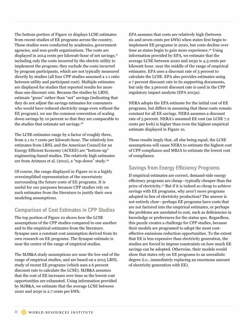
The bottom portion of Figure 10 displays LCSE estimates from recent studies of EE programs across the country. These studies were conducted by academics, government agencies, and non-profit organizations. The costs are displayed in 2014 cents per kilowatt-hour of net savings,27 including only the costs incurred by the electric utility to implement the program; they exclude the costs incurred by program participants, which are not typically measured directly by studies (all four CPP studies assumed a 1:1 ratio between utility and participant cost). Multiple estimates are displayed for studies that reported results for more than one discount rate. Because the studies by LBNL estimate “gross” rather than “net” savings (indicating that they do not adjust the savings estimates for consumers who would have reduced electricity usage even without the EE program), we use the common convention of scaling down savings by 10 percent so that they are comparable to the studies that estimate net savings.28

The LCSE estimates range by a factor of roughly three, from 2.1 to 7 cents per kilowatt-hour. The relatively low estimates from LBNL and the American Council for an Energy Efficient Economy (ACEEE) are “bottom-up” engineering-based studies. The relatively high estimates are from Arimura et al. (2012), a “top-down” study.29

Of course, the range displayed in Figure 10 is a highly oversimplified representation of the uncertainty surrounding the future costs of EE programs. It is useful for our purposes because CPP studies rely on such estimates from the literature to justify their own modeling assumptions.

Comparison of Cost Estimates in CPP Studies The top portion of Figure 10 shows how the LCSE assumptions of the CPP studies compared to one another and to the empirical estimates from the literature. Synapse uses a constant cost assumption derived from its own research on EE programs. The Synapse estimate is near the center of the range of empirical studies.

The MJB&A study assumptions are near the low end of the range of empirical studies, and are based on a 2015 LBNL study of recent EE programs (which uses a 6 percent discount rate to calculate the LCSE). MJB&A assumes that the cost of EE increases over time as the lowest cost opportunities are exhausted. Using information provided by MJB&A, we estimate that the average LCSE between 2020 and 2030 is 2.7 cents per kWh.

EPA assumes that costs are relatively high (between six and seven cents per kWh) when states first begin to implement EE programs in 2020, but costs decline over time as states begin to gain more experience.30 Using information provided by EPA, we estimate that the average LCSE between 2020 and 2030 is 4.3 cents per kilowatt-hour, near the middle of the range of empirical estimates. EPA uses a discount rate of 3 percent to calculate the LCSE. EPA also provides estimates using a 7 percent discount rate in its supporting documents, but only the 3 percent discount rate is used in the CPP regulatory impact analysis (EPA 2015a).

NERA adopts the EPA estimate for the initial cost of EE programs, but differs in assuming that these costs remain constant for all EE savings. NERA assumes a discount rate of 5 percent. NERA’s assumed EE cost (an LCSE 7.2 cents per kwh) is higher than even the highest empirical estimate displayed in Figure 10.

These results imply that, all else being equal, the LCSE assumptions will cause NERA to estimate the highest cost of CPP compliance and MBJA to estimate the lowest cost of compliance.

Savings from Energy Efficiency Programs If empirical estimates are correct, demand-side energy efficiency programs are cheap—typically cheaper than the price of electricity.31 But if it is indeed so cheap to achieve savings with EE programs, why aren’t more programs adopted in lieu of electricity production? The answer is not entirely clear—perhaps EE programs have costs that are not factored into the empirical estimates, or perhaps the problems are unrelated to cost, such as deficiencies in knowledge or preferences for the status quo. Regardless, this puzzle creates a challenge for CPP studies, because their models are programed to adopt the most cost-effective emissions reduction opportunities. To the extent that EE is less expensive than electricity generation, the studies are forced to impose constraints on how much EE savings can be adopted. Otherwise, their models would show that states rely on EE programs to an unrealistic degree (i.e., immediately replacing an enormous amount of electricity generation with EE).



In the context of CPP studies, this implies the need for further assumptions relating to two important questions (in addition to the assumptions on EE program costs, described above). First, what is the trajectory of future EE savings in the absence of the CPP (referred to as a “baseline” EE forecast)? Second, how much incremental EE saving is caused by the CPP? Assumptions about EE savings under baseline and CPP policy scenarios will influence estimates of the cost of CPP compliance.

Recent Trends and Projections for Baseline EE Savings (in the Absence of the CPP) We begin with baseline EE savings. Recent historical data and forecasts from LBNL enable us to identify a range of assumptions for the future trajectory of EE savings in the absence of the CPP.

The prevalence of EE programs in the United States has increased rapidly in the past decade, as the financial and environmental benefits of encouraging reduced electricity consumption have become more apparent. A few states have lowered their EE ambitions in recent years,32 but, overall, the national trend is toward increased spending

and savings. EE program funding by electric utilities increased roughly fourfold between 2006 and 2013, from $1.6 to $6.3 billion.33

Each year, ACEEE releases its “Energy Efficiency Scorecard” study, which includes estimates of the level of total EE savings from new utility-funded EE programs across the country that year. The solid black line in Figure 11 shows estimated nationwide savings from new EE programs implemented between 2006 and 2014 (the “incremental annual savings” displayed in the figure exclude the savings still accruing from programs implemented in prior years).34 The 24 TWh of savings in 2013 represented 0.67 percent of nationwide retail electricity sales—LBNL reported an almost identical figure in its 2013 study of nationwide EE savings (Barbose et al. 2013).

These national estimates include large variation at the state level—from 0 to roughly 2 percent of retail sales. EE programs and the associated savings are concentrated in West Coast and northeastern states, suggesting there are still considerable opportunities for EE programs to expand into new regions of the country.

Figure 11 | Historical Estimates and Forecasts of Savings from New Utility-Funded EE Programs

Historical Data (ACEEE)

LBNL Projection: HIGH

LBNL Projection: MID

LBNL Projection: LOW

Incr

emen

tal A

nnua

l Sav

ings

(TW

h)

45

40

35

30

25

20

15

10

5

0

2006 2007 2008 2009 2010 2011 2012 2013 2014 2015 2016 2017 2018 2019 2020 2021 2022 2023 2024 2025

Sources: ACEEE 2015; LBNL projections from Barbose et al. 2013.

24 |

the NERA study also shows savings dropping to zero with one exception: NERA assumes new EE savings in California used for compliance with AB 32, and these are included in its baseline scenario. California is projected to achieve roughly 2.7 TWh of new EE savings each year between 2020 and 2030, according to EPA. In all other states, NERA assumes that EE savings fall to zero in the absence of the CPP.

The baseline scenario in the Synapse study assumes that states will comply with Energy Efficiency Resource Standards (EERS) already on the books. In all states without EERS, savings from new EE programs are assumed to fall to zero (or remain at zero). As shown in Figure 12, this implies significantly higher levels of EE savings compared to the other CPP studies; nevertheless, it implies a lower level of savings than even the “LOW” baseline forecast of LBNL.

None of the studies offer a justification for sharp reductions in new EE savings in the absence of the CPP. It seems likely that baseline savings are underestimated in these studies (with the possible exception of the Synapse study), which has multiple consequences for their results. First, it leads to overestimates of baseline electricity use and thus baseline emissions. This makes any given emissions target appear more stringent and thus more expensive to achieve. Second—and perhaps more importantly, as explained below—assuming little to no savings in the “baseline scenario” implies that all savings assumed to be achieved in the “policy scenario” are caused by the CPP. Consequently, more EE savings are likely being attributed to the CPP than is warranted. This underscores the importance of the point made above, that the modeling community should pay more attention going forward to generating plausible forecasts of EE savings under various policy scenarios, despite the difficulties of doing so.

CPP Scenario EE Forecasts For many reasons, the CPP may encourage states to adopt EE programs in addition to those that would have occurred in the absence of the regulation. First, by requiring states to achieve the CPP targets, it forces them to look for ways to lower emissions cost-effectively,

We found only one comparable forecast of the future trajectory of nationwide EE savings that was available in 2015. A 2013 LBNL study provides three trajectories of EE savings from new programs implemented in 2015, 2020, and 2025 (Barbose et al. 2013). These trajectories are displayed in Figure 11 using dotted lines, with linear extrapolation between the estimated years. According to LBNL, none of the three scenarios contemplate the additional incentives for EE provided by new EPA climate regulations such as the CPP.35

LBNL’s “LOW” scenario assumes that EE program savings remain relatively flat at a level just above its historical savings estimate for 2010. Given the savings achieved in 2011 through 2014, this scenario appears pessimistic, at least in the short run. The “MID” scenario shows new EE savings continuing to grow, but at a far slower pace than in recent years—this scenario accounts for meeting state-level legislative targets already in place. The “HIGH” scenario assumes energy efficiency plays a more prominent role in state and utility resource planning going forward, and states are assumed to follow the examples of the “leading” EE states in their regions. Given recent savings levels, this scenario appears optimistic in the near term.

The lack of forecasts on the future of EE programs is a real concern for the energy modeling community. EE is widely regarded as a key mechanism for achieving emissions reductions, so future emissions pathways cannot be estimated with much precision absent a strong understanding of the future of EE efforts. Going forward, more attention should be focused on forecasting EE savings under various policy scenarios.

Baseline EE Forecasts in CPP StudiesThe CPP studies all assume that savings from EE programs will fall substantially in the absence of the CPP. The top graph in Figure 12 displays the three estimates of baseline annual EE savings (from new programs) compared to historical estimates and the LBNL forecasts. Three of the studies find savings from new EE programs falling to or near zero in the absence of the CPP, despite recent trends and state policies that require considerable new EE savings.36 In the EPA and MJB&A studies, savings from new EE programs are assumed to fall to zero, while



perhaps for the first time. Second, for states that set up cap-and-trade programs, emissions allowances (or auction revenue) can be used to fund EE programs. Third, in states where the CPP causes the price of electricity to increase, EE programs become more cost-effective than they were prior to the CPP. Finally, the CPP explicitly incentivizes states to implement energy efficiency programs in low-income communities in 2020 and 2021 by providing them with credits that can be used toward achieving the emissions targets in later years.

While the mechanisms described above are not explicitly reflected in the CPP studies, each study assumes that the CPP will cause a significant amount of new savings from EE programs.37 The middle graph in Figure 12 displays the assumed EE savings caused by the CPP, and the bottom graph displays total EE savings (equal to baseline savings plus savings caused by the CPP).

Despite the significant savings from new EE programs in recent years (~25 TWh in 2014), EPA assumes zero savings from new EE programs between 2015 and 2019. EPA assumes that savings ramp up starting in 2020 and, by the mid-2020s, EE savings reach a level comparable to (but still lower than) LBNL’s “High” baseline forecast.38

NERA adopts the same assumptions as EPA except, as noted above, new EE savings in California are included in the baseline and thus are not assumed to be caused by the CPP.

The Synapse study displays two scenarios of new EE savings with the CPP in place. In its “Synapse-CPP” scenario, Synapse assumes that savings from new programs increase by about 7 TWh per year beginning in 2016, with the growth slowing in the mid-2020s. Savings from new EE programs in this scenario exceed 100 TWh per year starting in 2027. In its “Low-EE-CPP” scenario, savings from new EE programs are relatively constant at about 25 TWh per year until the early 2020s, at which point they ramp up to above 40 TWh in 2025 and thereafter (a level similar to LBNL’s baseline “HIGH” forecast).39

The MJB&A study provides various scenarios with respect to EE savings. In its “Modest EE” case, MJB&A adopts EPA’s assumption for EPA savings. MJB&A’s “Significant EE” case assumes that states can achieve much higher levels of EE savings over time—2 percent of total electricity demand instead of 1 percent. Based on information provided by MJB&A, we estimate that this assumption implies roughly 50 TWh of new EE savings per year. Due to MJB&A’s assumption of zero EE savings in its baseline, which was used to estimate effects of the CPP on electricity bills, the CPP is assumed to cause all of the savings from new EE programs.

Characterizing the EE Savings AssumptionsHow assumptions about EE savings affect the results of CPP studies is not immediately clear. If EE programs are less expensive than the cost of producing electricity (in other words, if it is cheaper to get consumers to stop using electricity than to provide them with that electricity), then assuming a greater level of EE savings leads to lower electricity bills. In that case, the assumption that more EE savings are caused by the CPP leads to the result that lower electricity bills are caused by the CPP.

The cost assumptions of the CPP studies imply that EE savings are cheap compared to electricity production.40 Therefore, the (likely) underestimates of baseline EE savings caused these studies to underestimate the effect of the CPP on electricity bills. As noted above, we cannot characterize the assumptions on EE savings in the studies’ CPP scenarios due to a lack of independent forecasts, so the net effects on study results of assumptions concerning EE savings are less clear.

Certain results of these CPP studies indicate that these assumptions are highly influential in the study’s overall conclusions. For example, the Synapse and MJB&A studies conclude that the CPP will significantly reduce electricity bills in scenarios that assume the CPP causes a large amount of new EE.

26 |

Figure 12 | EE Savings Assumptions in CPP Studies

LBNL Projection: HIGH

LBNL Projection: MID

LBNL Projection: LOW

Synapse (No CPP)

NERA Baseline (approx.)

EPA & MJB&A Baseline

Synapse (High-EE CPP)

MJB&A: Significant EE (approx.)

EPA & MJB&A: Modest EE

NERA (approx.)

Synapse (Low-EE CPP)

Synapse (High-EE CPP)

MJB&A: Significant EE (approx.)

Synapse (Low-EE CPP)

EPA & NERA & MJB&A (modest EE)

0

5

10

15

20

25

30

35

40

45

50

55

2020 2021 2022 2023 2024 2025 2026 2027 2028 2029 2030

Incr

emen

tal A

nnua

l Sav

ings

from

N

ew E

E Pr

ogra

ms

(TW

h)

0

10

20

30

40

50

60

70

80

90

2020 2021 2022 2023 2024 2025 2026 2027 2028 2029 2030

Incr

emen

tal A

nnua

l Sav

ings

from

N

ew E

E Pr

ogra

ms

(TW

h)

0

10 20 30 40 50 60

70 80

90 100 110 120

2020 2021 2022 2023 2024 2025 2026 2027 2028 2029 2030

Incr

emen

tal A

nnua

l Sav

ings

from

N

ew E

E Pr

ogra

ms

(TW

h)

'

Baseline EE Forecast

EE Caused by CPP

Total EE Forecast (Baseline + Caused by CPP)



4. NATURAL GAS PRICE FORECASTSNatural gas accounted for about 28 percent of total energy consumed in the United States in 2014, behind only petroleum as a leading source of energy (EIA 2015d). In the U.S. electricity sector, natural gas-fired electricity generation accounts for about one-third of total generation. But less than 40 percent of U.S. natural gas is used to produce electricity (EIA 2016)—the majority is used for heating buildings and homes, fueling vehicles, and powering industrial furnaces, among other uses. For that reason, the price of natural gas is determined by a wide range of factors, including the demand for electricity, heating, and the other goods and services dependent on natural gas, as well as the availability and cost of extracting and transporting the resource (EIA 2015e).

The future price of natural gas is one of the most important determinants of the costs of the CPP, and it is also one of the most uncertain. In this section, we first describe the role of natural gas in the U.S. power sector and how natural gas prices affect CPP compliance costs. Then, we review the literature on expert forecasts of the future price of natural gas and compare these forecasts to the assumptions

of the four CPP studies. Finally, we discuss the potential implications of these assumptions.

Natural Gas Prices and CPP Compliance Costs The effect of future natural gas prices on overall CPP compliance costs is not as straightforward as the effect of solar and wind costs. On the one hand, to meet the Clean Power Plan emissions (or emissions rate) targets, many states will shift generation from coal to natural gas power plants, which reduces emissions because burning natural gas produces roughly half as much carbon dioxide as burning coal.41 If natural gas plants are less expensive to operate due to lower fuel costs, this compliance alternative is less expensive.

On the other hand, natural gas is still a fossil fuel that causes significant greenhouse gas emissions, so states could also reduce emissions by shifting away from natural gas and toward zero-carbon generation options like solar and wind, or by reducing consumption of electricity that would have been produced by natural gas generation. In this situation, the effect of the assumed price of natural gas on CPP compliance costs is reversed, because lower natural gas prices make switching away from natural gas more costly.

Figure 13 | Henry Hub Natural Gas Spot Price, 1997–2013

Note: All prices have been adjusted to 2014 dollars.

Source: U.S. Energy Information Administration, “Henry Hub Natural Gas Spot Price,” release date: May 18, 2016, https://www.eia.gov/dnav/ng/hist/rngwhhdA.htm.

$0.00

$1.00

$2.00

$3.00

$4.00

$5.00

$6.00

$7.00

$8.00

$9.00

$10.00

1997 1998 1999 2000 2001 2002 2003 2004 2005 2006 2007 2008 2009 2010 2011 2012 2013

Dol

lars

per

Mill

ion

Btu

(201

4$)

https://www.eia.gov/dnav/ng/hist/rngwhhdA.htm

28 |

natural gas in the United States (Budzik 2014). Between 1997 and 2008, the price of gas nearly tripled, but it has since dropped to near pre-2000 levels. These national annual average prices mask more significant regional and temporal variation.

As in previous sections, we compiled expert forecasts on future Henry Hub natural gas prices available in 2015, which are displayed in Figure 14 along with the corresponding recent historical prices. The projections come from a variety of sources including government agencies, private consulting firms, and financial advisory companies. We made no attempt to assess the forecasts in terms of rigor or expertise. We simply adjusted the forecasts into comparable terms (2014 dollars), and we used a linear extrapolation for any intermediate years omitted from the forecasts. In some cases, these projections may be accounting for the expected effect of the CPP, making this an imperfect comparison with the baseline assumptions in the CPP studies.

Figure 14 shows the expert consensus that natural gas prices will increase gradually from the 2015 average

Two additional points are worth noting. First, we focus on the price of natural gas rather than the cost of building a natural gas power plant primarily because the CPP regulates emissions from existing (rather than new) fossil fuel power plants.42 Second, two prices of natural gas are relevant to a detailed energy sector forecast: the assumed natural gas price in the absence of the CPP (the baseline scenario price) and the natural gas price that results from the changes in supply and demand due to the CPP. While both of these prices affect CPP compliance costs, we focus on the baseline scenario natural gas prices because these are inputs to CPP studies (rather than outputs that result from running the model), and thus reflect a more explicit assumption made by the study authors.43

Recent Trends and Expert Forecasts of Natural Gas PricesNatural gas prices have fluctuated dramatically in the past decade due to advances in drilling techniques, extreme weather, regional transportation constraints, and economic turmoil, among other factors. Figure 13 shows prices at Henry Hub in Louisiana, which is a major domestic distribution hub and the most common pricing point for

Figure 14 | Expert Forecasts of Henry Hub Natural Gas Prices

Sources: EIA 2015c; BNEF (Culver 2015); Cedigaz 2015; Deloitte 2015; NWPCC 2014; Moody’s Investors Service 2015; GLJ Petroleum Consultants 2014; World Bank 2015; AEO 2015, IHSGI, EVA, and ICF price forecasts are those reported in EIA (2015c).

Historical (EIA)

ICF

NWPCC (Medium case scenario)

GLJ Petroleum Consultants Ltd

AEO 2015

Moody’s Investors Service

World Bank

Cedigaz

IHSGI

BNEF (high oil price and LNG case)

EVA

Deloitte

BNEF (low oil price and LNG case)

$2.00

$3.00

$4.00

$5.00

$6.00

$7.00

$8.00

$9.00

$10.00

2007 2008 2009 2010 2011 2012 2013 2014 2015 2016 2017 2018 2019 2020 2021 2022 2023 2024 2025 2026 2027 2028 2029 2030

2014

dol

lars

per

MM

BTU



price of $2.61 per million Btu,44 although the pace of this expected increase differs to some extent. In 2025, forecasts range from roughly $4 to $6 per million Btu. By 2030, these predictions differ more significantly, ranging from $4 to $8 per million Btu.

The forecasts displayed in Figure 14 fall into a relatively narrow range, given the wide swings in natural gas prices in recent years—none predict that average annual prices will rise higher than 2008 levels or lower than current levels through 2030.

Natural Gas Price Forecasts from CPP Studies Despite the uncertainty surrounding natural gas price forecasts, studies typically assume a single trajectory of future Henry Hub natural gas prices (in the absence of

the CPP). Recent expert projections are the best reference available to put the assumptions on natural gas prices from CPP studies into context. Figure 15 compares the assumed baseline Henry Hub natural gas prices in the four CPP studies.45

NERA and Synapse both adopt the price forecasts from the AEO 2015 report, which is based on detailed supply and demand projections from EIA’s National Energy Modeling System. EPA and MJB&A use forecasts embedded in IPM, a detailed power sector model. The price trajectories are similar—EPA/MJB&A assume that natural gas prices are somewhat higher than projected by the other two studies in the early and late 2020s, and somewhat lower in the mid-2020s.

Figure 15 | Baseline Henry Hub Natural Gas Price Assumptions in CPP Studies

NERA & Synapse

EPA & MJB&A

$3.00

$3.50

$4.00

$4.50

$5.00

$5.50

$6.00

$6.50

$7.00

2020 2021 2022 2023 2024 2025 2026 2027 2028 2029 2030

Dol

lars

per

MM

Btu

(201

4$)

30 |

Figure 16 compares the assumptions of the CPP studies (top portion) to the expert forecasts (bottom portion) for the year 2022, the first year of CPP implementation. The CPP studies all fall at the higher end—but well within the range of—expert forecasts. Note that, in the years 2024 to 2026, the Synapse and NERA assumptions are higher than the EPA and MJB&A assumptions, as displayed in Figure 15.

The similarities in assumptions among the CPP studies and the expert forecasts indicate that it is unlikely that natural gas prices were a major cause of the differences in the results of the CPP studies.

5. STRUCTURE OF STATE IMPLEMENTATION PLANSThe CPP offers states considerable flexibility in how to achieve their targets. The choices that states must make in crafting implementation plans include the following:

▪ Whether power plants must achieve standards individually or on average across a fleet

▪ Whether to use renewable energy and energy efficiency programs to help meet the standards

▪ Whether to adopt the “mass-based” (based on aggregate emissions) or “rate-based” (based on emissions per quantity of generation) targets

▪ Whether to use a market-based approach like emissions allowance trading or an emissions fee

▪ If adopting a mass-based target, whether to include new as well as existing power plants

▪ Whether to meet the state targets alone or cooperate with other states in terms of shared targets, emissions trading, or procurement of renewable energy or energy efficiency resources

▪ How to allocate or auction any emissions allowances, if applicable

While many states have begun their planning processes, with the CPP on hold during the court case, none have made a final decision regarding the issues listed above. This gives CPP studies substantial latitude to make assumptions about how states will choose to comply with the targets. All else being equal, assuming that states choose implementation plans with less stringent targets will cause models to estimate lower CPP compliance costs. For example, if, for a given state, a “mass-based” target is less stringent (and therefore less costly to achieve) than a rate-based target, assuming that the state will elect to meet the mass-based target will lead to lower cost estimates.

In addition, assuming that states allow for more flexibility in how emissions reductions are achieved tends to lower estimates of CPP compliance costs. In what follows,

Figure 16 | Henry Hub Natural Gas Prices, 2022 (2014$ per Million Btu)

Lower CPP Costs

Higher CPP Costs

2022 Henry Hub Natural Gas Prices (2014$ per MMBtu)

$4.09Deloitte

$4.10World Bank

$4.27BNEF

(low oil price)

$4.18IHSGI

$4.54BNEF

(high oil price)

$5.20AEO 2015

$5.33ICF

$5.41NWPCC

$5.51EVA

$5.83Cedigaz



$5.46$5.20

Sources: Deloitte 2015; World Bank 2015; IHSGI (EIA 2015c); BNEF (Culver 2015); AEO (EIA 2015c); ICF (EIA 2015c); NWPCC 2014; EVA (EIA 2015c); Cedigaz 2015.



we provide an illustrative example of this point—the assumed degree of geographic cooperation among states in meeting their targets.

Multi-state Cooperation in Achieving CPP TargetsStates can cooperate with one another to achieve their targets in multiple ways. They can formally merge their mass-based or rate-based targets so that the combined region has one target to achieve. They can agree to allow trading of emissions allowances or emissions rate credits between entities across state lines. Or, they can allow regulated entities to procure credits for energy efficiency programs or renewable energy generation from outside of the state.46

Increased cooperation among states will lead to decreased estimates of overall compliance costs for the cooperating multi-state region. To see why, consider the illustrative example of two states, State A and State B, that are required to reduce their emissions by either 10 units each (a “Without Cooperation Scenario”) or 20 units collectively (a “Cooperation Scenario”). Further assume that the states are identical except that relative to State A, State B has far more low-cost opportunities to reduce emissions.

Of course, the total costs of emissions reductions are far lower in the Cooperation Scenario, because the states take advantage of the cost-effective emissions reduction opportunities in State B, and State B reduces its emissions by more than 10 units. In the Without Cooperation scenario, both states are forced to reduce emissions by 10 units, so the total costs are greater due to the more expensive actions that State A is forced to take. State A would prefer to compensate State B to take on a greater share of the emissions reductions in the Without Cooperation, but it is not able to do so.

This example is of course oversimplified, but the principle it illustrates is highly relevant to CPP studies. For any multi-state region, the set of least-cost actions to reduce emissions will not exactly coincide with the emissions reduction responsibilities of each state, so cooperation among states reduces the cost of achieving the emissions targets.47

Assumptions of CPP Studies on Multi-state Cooperation Figure 17 summarizes the CPP studies with respect to their degree of assumed multi-state cooperation. As explained above, assuming a greater degree of cooperation will

Figure 17 | Assumed Geographic Cooperation in CPP State Implementation Plans

Lower CPP Costs

Higher CPP Costs

Assumed Geographic Cooperation in CPP State Implementation Plans

Most scenarios assume two trading regions

One scenario with three clean energy procurement regions

Two trading regions


Nationwide Cooperation to Achieve Targets

Limited regional cooperation

States Achieve Targets Alone

Substantial regional cooperation

One scenario assumes limited trading

One scenario with six trading regions


32 |

tend to lower overall CPP costs, whereas assuming less cooperation raises CPP costs. Because of the qualitative nature of “cooperation,” our characterization of these studies across the spectrum is necessarily somewhat more subjective compared to the quantitative characterizations provided in previous sections.

The EPA Regulatory Impact Analysis features two scenarios. One requires that all states meet their mass-based standards individually, with no cooperation or trading among states. In EPA’s second scenario, a high degree of cooperation is assumed with respect to the procurement of renewable energy generation and demand-side energy efficiency programs. Specifically, renewable energy or energy efficiency can be used to meet state targets within the regions of the country’s three large electricity grid interconnections (eastern states, western states, and Texas). Trading of emissions allowances is not permitted between states in either scenario. The absence of trading among states is an extremely unrealistic outcome; after all, EPA is encouraging interstate trading, many states have expressed interest in trading with others, and nine northeastern states already allow interstate CO2 emissions trading under the Regional Greenhouse Gas Initiative.

The NERA study features two scenarios as well. Like EPA, one scenario assumes no cooperation among states, so each state has to meet its mass-based targets individually. The second scenario allows trading of emissions allowances within six regions of the country. In effect, within each of these six multi-state regions, the mass-based targets are met collectively.

The Synapse study features a single scenario that enables states to trade within two groups across the country: the nine northeastern states in the Regional Greenhouse Gas Initiative (RGGI), and all other states. The mass-based targets are met collectively across the two multi-state regions. The Synapse study is thus more optimistic in its assumption regarding inter-state cooperation than either the NERA or EPA study.

Finally, the MJB&A study includes four scenarios that provide estimates of the CPP’s effects on electricity bills, three of which assume nationwide trading among states with the exception of California. One scenario assumes trading can occur only between the nine northeastern states that comprise the Regional Greenhouse Gas Initiative.

6. SUMMARY AND COMPARISON OF CPP STUDY RESULTSIn this paper, we have provided an overview of certain key assumptions that influence forecasts of the costs of the CPP. For each assumption, we compiled information from the empirical literature and expert forecasts to develop a range of plausible modeling inputs for a CPP study. Then, we compared these ranges of modeling inputs to the corresponding assumptions used in the four CPP studies that have been released to date and contain sufficient information to undertake this comparison. The studies were conducted by the U.S. Environmental Protection Agency (EPA), NERA Economic Consulting, Synapse Energy Economics, and M.J. Bradley & Associates (MJB&A).

Table 1 summarizes the assumptions on which we focused, how these assumptions tend to affect CPP cost estimates, and the information we used to develop a range of plausible assumptions to which the inputs of the CPP studies could be compared.



Figure 18 shows how the inputs of the CPP studies compare to the corresponding ranges of inputs we developed for each assumption, which are depicted by the black lines. We omit savings from energy efficiency caused by the CPP because information was not available to develop a corresponding range, and we omit natural gas prices because the inputs of the CPP studies overlap multiple times over the CPP compliance period.

The CPP studies report their results somewhat differently, but each report contains some information on the effect of the CPP on average nationwide electricity bills, which can be seen as a proxy for overall CPP costs.

Figure 19 compares the findings across CPP studies on electricity bills, using the metric chosen by the study authors to display their own results. The NERA study

shows increases in electricity bills due to the CPP, EPA shows increases in bills in 2020 and decreases in 2030, and the Synapse and MJB&A studies show decreases in bills caused by the CPP.

Of course, many assumptions aside from those considered in this paper influence estimates of CPP costs. There are also important differences in the simulation models used for each CPP study—for example, while EPA, MJB&A, and Synapse use detailed power sector-only models, NERA’s model is an economy-wide model that captures interactions between sectors. Finally, the effect on the economy of the CPP is likely to include important factors outside the scope of all of these studies, such as the economic effects of air pollution, as explained in Box 1.

ASSUMPTION LIKELY EFFECTS ON CPP COSTSINFORMATION USED TO DEVELOP PLAUSIBLE RANGE OF ASSUMPTIONS

Cost of solar energy plants Higher solar costs lead to higher CPP costs Expert forecasts

Cost of wind energy plants Higher wind costs lead to higher CPP costs Expert forecasts

Cost of demand-side energy efficiency (EE) programs

Higher EE costs lead to higher CPP costs Empirical studies of past and current programs

Baseline savings from energy efficiency (without the CPP)

Smaller baseline savings lead to lower CPP costs (if EE is relatively inexpensive)

Forecasts from Lawrence Berkeley National Laboratory (Barbose et al. 2013)

Savings from energy efficiency caused by the CPP Greater savings lead to lower CPP costs (if EE is relatively inexpensive)

None available

Natural gas pricesAmbiguous (but likely that higher prices lead to higher CPP costs in most places)

Expert forecasts

Cooperation in state implementation plans More cooperation leads to lower CPP costsBounding scenarios (full cooperation to no cooperation)

Table 1 | Summary of CPP Study Assumptions, Effects on Costs, and Information Sources

34 |

The correlation between the CPP studies’ assumptions and results (with regard to their relative optimism/pessimism) is nevertheless unmistakable. The NERA study uses pessimistic assumptions related to the future of clean energy and the flexibility of implementation plans, and it arrives at the pessimistic result that the CPP increases electricity bills, whereas the MJB&A study uses far more optimistic assumptions and arrives at the far more optimistic result that the CPP will significantly reduce electricity bills. EPA’s assumptions are near the

middle of the ranges we developed (with the exception of baseline EE savings, where all four studies used low estimates), and its results are in the middle as well. This may indicate that either our selected assumptions are indeed strongly influencing the results of these studies and/or they are “canaries in the coalmine,” meaning that the tendency to use optimistic/pessimistic assumptions carried over to additional assumptions (not examined in this paper) that influence the studies’ results.

Figure 18 | Impact of CPP on Electricity Bills: Comparison of CPP Study Inputs and Ranges of Plausible Assumptions CPP Study Inputs vs Plausible Range of Assumptions

Solar PV Plant Costs

Wind Plant Costs

Energy Efficiency Program Costs

Baseline Energy Efficiency Savings

Cooperation in Implementation Plans

Low

er C

PP C

osts

Higher CPP Costs

Note: The black lines are representative of the ranges of plausible assumptions developed by WRI. We omit savings from energy efficiency caused by the CPP because information was not available to develop a corresponding range, and we omit natural gas prices because the inputs of the CPP studies overlap multiple times over the CPP compliance period.



These findings suggest that modeling can be used to justify highly positive or negative estimates of the CPP’s economic effects, depending on assumptions with respect to technological progress, commodity prices, and policy implementation. If true, this indicates that policymakers, judges, and the general public should be wary of accepting CPP cost estimates without consideration of their assumptions, because

the results of these studies may reflect the optimism or pessimism of the study assumptions rather than the inherent attributes of the regulation. They also omit the important effects of the policy that are difficult to capture in monetary terms. This paper is a first step in our effort to promote transparency and impartiality in economic impact studies.

Figure 19 | Impact of CPP on Electricity Bills: Comparison of CPP Study Findings

CPP Lowers Bills CPP Increases Bills

Retail electricity bills decrease 5-17% in 2030 for the

various scenarios displayed

Retail electricity bills increase 0-3% (annual averages 2022-2033)

Retail electricity bills increase 2-3% in 2020 and

decrease 7-8% in 2030

Residential electricity bills decrease

3-15% in 2030

CPP Studies Overall Results: Electricity Bills

Note: NERA electricity bill impacts are estimated using results for total generation and delivered electricity price.

36 |

REFERENCESAllcott, H., and M. Greenstone. 2012. “Is There an Energy Efficiency Gap?” Journal of Economic Perspectives 26(1): 3–28.

ACEEE (American Council for an Energy-Efficient Economy). 2009. “The Best Value for America’s Energy Dollar: A National Review of the Cost of Utility Energy Efficiency Programs.” Washington, DC: American Council for an Energy-Efficient Economy.

ACEEE. 2014. “The Best Value for America’s Energy Dollar: A National Review of the Cost of Utility Energy Efficiency Programs.” Washington, DC: American Council for an Energy- Efficient Economy.

ACEEE. 2015. “The 2015 State Energy Efficiency Scorecard.” Washington, DC: American Council for an Energy-Efficient Economy. http://aceee.org/state-policy/scorecard. URL includes link to previous years’ Energy Efficiency Scorecards.

Arimura, T.H., S. Li, R. Newell, and K. Palmer. 2012. “Cost-Effectiveness of Electricity Energy Efficiency Programs.” Energy Journal 33:(2), 63-99.

AWEA (American Wind Energy Association). 2015. “U.S. Wind Industry Leaders Praise Multi-year Extension of Tax Credits.” Washington, DC: AWEA. http://www.awea.org/MediaCenter/pressrelease.aspx?ItemNumber=8254.

Barbose, G.L., C.A. Goldman, I.M. Hoffman, and M. Billingsley. 2013. “The Future of Utility Customer-Funded Energy Efficiency Programs in the United States: Projected Spending and Savings to 2025.” Berkeley, CA: Lawrence Berkeley National Laboratory. https://emp.lbl.gov/sites/all/files/lbnl-5803e.pdf.

Barbose, G.L., and N. Darghouth. 2015. “Tracking the Sun VIII: The Installed Price of Residential and Non-Residential Photovoltaic Systems in the United States.” Berkeley, CA: Lawrence Berkeley National Laboratory. https://emp.lbl.gov/sites/all/files/lbnl-188238_1.pdf.

Bedilion, R. 2013. “Cost and Performance of Generation Technologies.” Palo Alto, CA: Electric Power Research Institute.

Bianco, N., K. Meek, R. Gasper, M. Obeiter, S. Forbes, and N. Aden. 2014. “Seeing is Believing: Creating a New Climate Economy in the United States.” Working Paper. Washington, DC: World Resources Institute. http://www.wri.org/sites/default/files/seeingisbelieving_working_paper.pdf.

BLS (Bureau of Labor Statistics). 2015. “Current Population Survey.” Washington, DC: U.S. Department of Labor. http://www.bls.gov/cps/#data.

Bolinger, M., and J. Seel. 2015. “Utility-Scale Solar 2014.” Berkeley, CA: Lawrence Berkeley National Laboratory. https://emp.lbl.gov/sites/all/files/lbnl-1000917.pdf.

Budzik, P. 2014. “U.S. Natural Gas Markets: Relationship between Henry Hub Spot Prices and U.S. Wellhead Prices.” Washington,

DC: U.S. Energy Information Administration. http://www.eia.gov/oiaf/analysispaper/henryhub/pdf/henryhub.pdf.

Cedigaz. 2015. “Medium and Long Term Natural Gas Outlook.” Paris, France: Cedigaz (International Association for Natural Gas). http://www.cedigaz.org/documents/2015/CEDIGAZProspects2015.pdf.

Channell, J., H.R. Jansen, A.R. Syme, S. Savvantidou, E.L. Morse, and A. Yuen. 2013. “Energy Darwinism: The Evolution of the Energy Industry.” Citi GPS. http://www.growsolar.org/wp-content/uploads/2014/10/Energy-Darwinism-The-Evolution-of-the-Energy-Industry.pdf.

Culver, N. 2015. “The Cost Landscape of Solar and Wind.” Bloomberg New Energy Finance. Americas Insight PowerPoint Presentation. https://www.senate.mn/committees/2015-2016/ 3058_Committee_on_Environment_and_Energy/2015-1_BNEF_presentation_final.pdf.

Deloitte. 2015. “Deloitte Resource Evaluation and Advisory.” http://www2.deloitte.com/content/dam/Deloitte/ca/Documents/REA/ca-en-rea-data-summary-price-forecast-september-2015.pdf.

DOE (U.S. Department of Energy). 2012. “SunShot Vision Study.” Washington, DC: U.S. Department of Energy. http://energy.gov/sites/prod/files/2014/01/f7/47927.pdf.

DOE. 2015. 2014 Wind Technologies Market Report. Washington, DC: U.S. Department of Energy. http://energy.gov/sites/prod/files/2015/08/f25/2014-Wind-Technologies-Market-Report-8.7.pdf.

EIA (U.S. Energy Information Administration). 2015a. “Levelized Cost and Levelized Avoided Cost of New Generation Resources in the Annual Energy Outlook 2015.” Washington, DC: U.S. Department of Energy. https://www.eia.gov/forecasts/aeo/electricity_generation.cfm.

EIA. 2015b. “California First State to Generate More than 5% of Electricity from Utility-Scale Solar.” Today in Energy. Washington, DC: U.S. Department of Energy. http://www.eia.gov/todayinenergy/detail.cfm?id=20492.

EIA. 2015c. “Annual Energy Outlook 2015.” Washington, DC: U.S. Department of Energy. http://www.eia.gov/forecasts/aeo/pdf/0383(2015).pdf.

EIA. 2015d. “Energy in Brief.” Washington, DC: U.S. Department of Energy. http://www.eia.gov/energy_in_brief/article/major_energy_sources_and_users.cfm.

EIA. 2015e. “Natural Gas Explained: Factors Affecting Natural Gas Prices.” Washington, DC: U.S. Department of Energy. Last updated July 28, 2015. https://www.eia.gov/energyexplained/index.cfm?page=natural_gas_factors_affecting_prices.

EIA. 2016. “Natural Gas Consumption by End Use.” Release date April 29, 2016. https://www.eia.gov/dnav/ng/ng_cons_sum_dcu_nus_a.htm.

http://www.awea.org/MediaCenter/pressrelease.aspx?ItemNumber=8254

http://www.awea.org/MediaCenter/pressrelease.aspx?ItemNumber=8254

https://emp.lbl.gov/sites/all/files/lbnl-188238_1.pdf

https://emp.lbl.gov/sites/all/files/lbnl-188238_1.pdf

http://www.wri.org/sites/default/files/seeingisbelieving_working_paper.pdf

http://www.wri.org/sites/default/files/seeingisbelieving_working_paper.pdf

http://www.bls.gov/cps/#data

https://emp.lbl.gov/sites/all/files/lbnl-1000917.pdf

https://emp.lbl.gov/sites/all/files/lbnl-1000917.pdf

http://www.eia.gov/oiaf/analysispaper/henryhub/pdf/henryhub.pdf

http://www.eia.gov/oiaf/analysispaper/henryhub/pdf/henryhub.pdf

http://www.cedigaz.org/documents/2015/CEDIGAZProspects2015.pdf

http://www.cedigaz.org/documents/2015/CEDIGAZProspects2015.pdf

http://www.growsolar.org/wp-content/uploads/2014/10/Energy-Darwinism-The-Evolution-of-the-Energy-Industry.pdf



https://www.senate.mn/committees/2015-2016/3058_Committee_on_Environment_and_Energy/2015-1_BNEF_presentation_final.pdf



http://www2.deloitte.com/content/dam/Deloitte/ca/Documents/REA/ca-en-rea-data-summary-price-forecast-september-2015.pdf

http://www2.deloitte.com/content/dam/Deloitte/ca/Documents/REA/ca-en-rea-data-summary-price-forecast-september-2015.pdf

http://energy.gov/sites/prod/files/2014/01/f7/47927.pdf

http://energy.gov/sites/prod/files/2014/01/f7/47927.pdf

http://energy.gov/sites/prod/files/2015/08/f25/2014-Wind-Technologies-Market- Report-8.7.pdf

http://energy.gov/sites/prod/files/2015/08/f25/2014-Wind-Technologies-Market- Report-8.7.pdf

https://www.eia.gov/forecasts/aeo/electricity_generation.cfm

https://www.eia.gov/forecasts/aeo/electricity_generation.cfm

http://www.eia.gov/todayinenergy/detail.cfm?id=20492

http://www.eia.gov/todayinenergy/detail.cfm?id=20492

http://www.eia.gov/forecasts/aeo/pdf/0383(2015).pdf

http://www.eia.gov/forecasts/aeo/pdf/0383(2015).pdf

http://www.eia.gov/energy_in_brief/article/major_energy_sources_and_users.cfm

http://www.eia.gov/energy_in_brief/article/major_energy_sources_and_users.cfm

https://www.eia.gov/energyexplained/index.cfm?page=natural_gas_factors_affecting_prices

https://www.eia.gov/energyexplained/index.cfm?page=natural_gas_factors_affecting_prices

https://www.eia.gov/dnav/ng/ng_cons_sum_dcu_nus_a.htm

https://www.eia.gov/dnav/ng/ng_cons_sum_dcu_nus_a.htm



EPA (U.S. Environmental Protection Agency). 2011. “The Benefits and Costs of the Clean Air Act from 1990 to 2020.” Washington, DC: U.S. Environmental Protection Agency.

EPA. 2015a. “Regulatory Impact Analysis for the Proposed Carbon Pollution Guidelines for Existing Power Plants and Emission Standards for Modified and Reconstructed Power Plants.” Washington, DC: U.S. Environmental Protection Agency.

EPA. 2015b. “Demand-Side Energy Efficiency Technical Support Document.” Released August 2015. https://www.epa.gov/sites/production/files/2015-11/documents/tsd-cpp-demand-side-ee.pdf.

Farese, P., R. Gelman, and R. Hendron. 2012. “A Tool to Prioritize Energy Efficiency Investments.” Golden, CO: National Renewable Energy Laboratory. http://www.nrel.gov/docs/fy12osti/54799.pdf.

Gillingham, K., R. Newell, and K. Palmer. 2006. “Retrospective Examination of Demand-Side Energy Efficiency Policies.” Annual Review of Environment and Resources 31: 161–192.

GLJ Petroleum Consultants. 2014. "Price Charts." https://www.gljpc.com/price-charts.

Greentech Media. 2015. Personal Communication with MJ Shiao, Director of Solar Research. November 10.

Hoffman, I.M., G. Rybka, G. Levetis, C.A. Goldman, L. Schwartz, M. Billingsley, and S. Schiller. 2015. “The Total Cost of Saving Electricity through Utility Customer-Funded Energy Efficiency Programs: Estimates at the National, State, Sector and Program Level.” Berkeley, CA: Lawrence Berkeley National Laboratory. https://emp.lbl.gov/sites/all/files/total-cost-of-saved-energy.pdf.

IEA (International Energy Agency). 2015. “World Energy Outlook 2015.” Paris, France: IEA. http://www.worldenergyoutlook.org/weo2015/#d.en.148701.

IRENA (International Renewable Energy Agency). 2012. “Renewable Energy Technologies: Cost Analysis Series. Wind Power.” Abu Dhabi, UAE: IRENA. https://www.irena.org/documentdownloads/publications/re_technologies_cost_analysis-wind_power.pdf.

Meyer, R. 2015. “How Solar and Wind Got So Cheap, So Fast.” Newsweek, December 6, 2015. http://www.newsweek.com/how-solar-and-wind-got-so-cheap-so-fast-401450.

M.J. Bradley & Associates. 2016. “EPA’s Clean Power Plan. Summary of IPM Modeling Results.” http://www.mjbradley.com/sites/default/files/MJBA_CPP_IPM_Summary.pdf.

Moody’s Investors Service. 2015. “Moody’s Lowers Oil Price Assumptions on Oversupply and Weakening Demand.” Global Credit Research. https://www.moodys.com/research/Moodys-lowers-oil-price-assumptions-on-oversupply-and-weakening-demand--PR_336879.

NC Sustainable Energy Association. 2012. “Levelized Cost of Solar Photovoltaics in North Carolina.” Raleigh, NC: NC Sustainable Energy Association.

NERA Economic Consulting. 2015. “Energy and Consumer Impacts of EPA’s Clean Power Plan.” White Plains, NY: NERA Economic Consulting. http://www.americaspower.org/wp-content/uploads/2015/11/NERA-CPP-Final-Nov-7.pdf.

North American Wind Power. 2015. “Study: Western Grid Can Withstand Disturbances under High Renewables Penetration.” http://www.nawindpower.com/e107_plugins/content/content.php?content.14254.

NREL (National Renewable Energy Laboratory). 2015. “Annual Technology Baseline (ATB) Spreadsheet.” Golden, CO: NREL. http://www.nrel.gov/analysis/data_tech_baseline.html.

NWPCC (Northwest Power and Conservation Council). 2014. “Revised Fuel Price Forecasts for the Seventh Power Plan.” Portland, OR: Northwest Power and Conservation Council. https://www.nwcouncil.org/media/7113626/Council-FuelPriceForecast-2014.pdf.

Obeiter, M., and C. Weber. 2015. “Reducing Methane Emissions from Natural Gas Development: Strategies for State-level Policymakers.” Washington, DC: World Resources Institute.

Olson, A., N. Schlag, K. Patel, and G. Kwok. 2014. “Capital Cost Review of Generation Technologies.” San Francisco, CA: Energy and Environmental Economics, Inc. https://www.wecc.biz/Reliability/2014_TEPPC_Generation_CapCost_Report_E3.pdf.

Short, W., P. Sullivan, T. Mai, M. Mowers, C. Uriarte, N. Blair, D. Heimiller, and A. Martinez. 2010. “Regional Energy Deployment System (ReEDS).” National Renewable Energy Laboratory Technical Report NREL/TP-6A20-46534. http://www.nrel.gov/analysis/reeds/documentation.html.

Solomon, D., and T. Tracy. 2011. “Obama Asks EPA to Pull Ozone Rule.” Wall Street Journal. Web. September 3. http://www.wsj.com/articles/SB10001424053111904716604576546422160891728.

Synapse Energy Economics. 2016. “Cutting Electric Bills with the Clean Power Plan. EPA’s Greenhouse Gas Reduction Policy Lowers Household Bills.” Cambridge, MA: Synapse Energy Economics. http://www.synapse-energy.com/sites/default/files/cutting-electric-bills-cpp-march2016.pdf.

The Brattle Group. 2015. “Comparative Generation Costs of Utility-Scale and Residential-Scale PV in Xcel Energy Colorado’s Service Area.” Cambridge, MA: The Brattle Group. http://brattle.com/system/publications/pdfs/000/005/188/original/Comparative_Generation_Costs_of_Utility-Scale_and_Residential-Scale_PV_in_Xcel_Energy_Colorado's_Service_Area.pdf?1436797265.

UCS (Union of Concerned Scientists). 2016. “Production Tax Credit for Renewable Energy.” http://www.ucsusa.org/clean_energy/smart-energy-solutions/increase-renewables/production-tax-credit-for.html#.Vmme9UpumUk.

World Bank. 2015. “World Bank Commodities Price Forecast.” Washington, DC: World Bank. http://www.worldbank.org/content/dam/Worldbank/GEP/GEPcommodities/Price_Forecast_20150722.pdf.

https://www.epa.gov/sites/production/files/2015-11/documents/tsd-cpp-demand-side-ee.pdf

https://www.epa.gov/sites/production/files/2015-11/documents/tsd-cpp-demand-side-ee.pdf

http://www.nrel.gov/docs/fy12osti/54799.pdf

https://www.gljpc.com/price-charts

https://emp.lbl.gov/sites/all/files/total-cost-of-saved-energy.pdf

http://www.worldenergyoutlook.org/weo2015/#d.en.148701

http://www.worldenergyoutlook.org/weo2015/#d.en.148701

https://www.irena.org/documentdownloads/publications/re_technologies_cost_analysis-wind_power.pdf

https://www.irena.org/documentdownloads/publications/re_technologies_cost_analysis-wind_power.pdf

http://www.newsweek.com/how-solar-and-wind-got-so-cheap-so-fast-401450

http://www.newsweek.com/how-solar-and-wind-got-so-cheap-so-fast-401450

http://www.mjbradley.com/sites/default/files/MJBA_CPP_IPM_Summary.pdf

http://www.mjbradley.com/sites/default/files/MJBA_CPP_IPM_Summary.pdf

https://www.moodys.com/research/Moodys-lowers-oil-price-assumptions-on-oversupply-and-weakening-demand--PR_336879



http://www.americaspower.org/wp-content/uploads/2015/11/NERA-CPP-Final-Nov-7.pdf

http://www.americaspower.org/wp-content/uploads/2015/11/NERA-CPP-Final-Nov-7.pdf

http://www.nawindpower.com/e107_plugins/content/content.php?content.14254

http://www.nawindpower.com/e107_plugins/content/content.php?content.14254

http://www.nrel.gov/analysis/data_tech_baseline.html

https://www.nwcouncil.org/media/7113626/Council-FuelPriceForecast-2014.pdf

https://www.nwcouncil.org/media/7113626/Council-FuelPriceForecast-2014.pdf

https://www.wecc.biz/Reliability/2014_TEPPC_Generation_CapCost_Report_E3.pdf

https://www.wecc.biz/Reliability/2014_TEPPC_Generation_CapCost_Report_E3.pdf

http://www.nrel.gov/analysis/reeds/documentation.html

http://www.nrel.gov/analysis/reeds/documentation.html

http://www.wsj.com/articles/SB10001424053111904716604576546422160891728

http://www.wsj.com/articles/SB10001424053111904716604576546422160891728

http://www.synapse-energy.com/sites/default/files/cutting-electric-bills-cpp-march2016.pdf

http://www.synapse-energy.com/sites/default/files/cutting-electric-bills-cpp-march2016.pdf

http://brattle.com/system/publications/pdfs/000/005/188/original/Comparative_Generation_Costs_of_Utility-Scale_and_Residential-Scale_PV_in_Xcel_Energy_Colorado's_Service_Area.pdf?1436797265




http://www.ucsusa.org/clean_energy/smart-energy-solutions/increase-renewables/production-tax-credit-for.html#



http://www.worldbank.org/content/dam/Worldbank/GEP/GEPcommodities/Price_Forecast_20150722.pdf



38 |

ENDNOTES1. The benefits of the Clean Power Plan include reduced carbon dioxide

emissions, which are the primary cause of climate change, as well as reduced local air pollution and its associated health impacts.

2. Solomon and Tracy 2011.

3. See, for example, http://www.cnn.com/2016/12/13/politics/kfile-scott-pruitt-climate-change-epa/.

4. U.S. Code Title 42, Chapter 85, Subchapter I, Part A, § 7411, “Standards of Performance for New Stationary Sources,” https://www.law.cornell.edu/uscode/text/42/7411.

5. Estimate from LBNL’s Utility Scale Solar 2014 report, released September 2015. This estimate reflects the median cost of projects installed in 2013, displayed in 2014 dollars per watt (direct current).

6. EPA and MJB&A use NREL’s “MID” scenario estimate from its draft 2015 Annual Technology Baseline. This estimate was revised downward in the final version of the study, which is the NREL estimate displayed in Figure E-2.

7. The “50% Price Decline” scenario from DOE (2012), per communication with Synapse authors.

8. Estimate from DOE’s "2014 Wind Technologies Market Report," released in August 2015. This estimate reflects the capacity-weighted average of wind plants installed in 2014 with capacity larger than 100 kW (DOE 2015).

9. Some studies also included state-specific capital cost adjustments for solar and wind.

10. The average price of retail electricity across all sectors in 2015 was 10.4 cents per kilowatt-hour, according to the U.S. Energy Information Administration. Each of the CPP studies assumes that the costs to participants in EE programs are equal to the cost to utilities, so the total program cost is twice the assumed cost to utilities displayed in the figure.

11. One of the modeling organizations objected to our attribution of causation to the differences between the baseline scenarios (forecasts without the CPP) and the policy scenarios (forecasts with the CPP). In the view of that modeling organization, the policy scenarios represented just one of many possible compliance pathways.

12. By relying on EIA’s AEO 2015 Reference Case projections of electricity demand, EPA may be implicitly accounting for a small amount of new EE in its demand forecast. However, to arrive at its CPP policy scenario, it adds the cost of all new EE and it subtracts the savings from all new EE when constructing its baseline scenario. It therefore seems most accurate to characterize the EPA study as assuming that all new EE is incremental to its baseline scenario, despite this disconnect in its modeling. The MJB&A study includes a secondary baseline that assumes new EE remains at current levels as opposed to falling to zero EE. But the study shows the effects of the CPP on electricity bills only in its primary baseline with no new EE, so this is baseline on which we focus.

13. Data from U.S. Energy Information Administration, “Henry Hub Natural Gas Spot Price,” release date, May 18, 2016, https://www.eia.gov/dnav/ng/hist/rngwhhdA.htm.

14. Section 111 of the Clean Air Act directs EPA to take costs into consideration when determining the extent to which emissions should be reduced. See U.S. Code Title 42, Chapter 85, Subchapter I, Part A, §

7411, “Standards of Performance for New Stationary Sources,” https://www.law.cornell.edu/uscode/text/42/7411.

15. One scenario assumed that all states elected to achieve their “mass-based” (i.e., CO2

emissions levels) targets, while the other scenario assumed that all states elected “rate-based” (i.e., CO

2 emissions rates)

targets. There are other differences between the scenarios, including the degree of cooperation among states with respect to procurement of renewable energy resources.

16. Information on funding per communication with MJB&A study author in May 2016. Following the completion of our analysis, MJB&A released a new CPP analysis in June 2016, the contents of which are not reflected in this document.

17. The intermittency of renewable energy sources is also a major concern at higher penetration rates. However, as long as solar and wind represent just a small percentage of total generation on the grid, this is much less of a concern. EPA modeling suggests that, with the Clean Power Plan, solar and wind combined will provide less than 10 percent of total U.S. electricity generation in 2030 (EPA 2015a).

18. Solar PV technology differs from concentrated solar power (or “solar thermal”), which concentrates sunlight to create heat, which is used to turn a generator to produce electricity.

19. Inverters convert the direct current produced by solar PV into the alternating current used by the grid.

20. A common concern regarding solar energy is whether there are limits to how much the electricity grid can rely on intermittent generation like solar. Simply put, can we rely on solar to provide a stable source of electricity generation given that the sun is not always shining? Indeed, one recent study showed that system stability may be jeopardized once renewable energy comprises about half of the generation on the grid (North American Wind Power 2015). But we can safely disregard those concerns for our purposes. Solar PV comprised less than 1 percent of U.S. electricity generation in 2014, and 5 percent in California, which is the largest percentage of any U.S. state (EIA 2015b). In addition, the improvements in storage and “smart grid” technologies may make intermittency less of a concern in the future, even at high penetration rates.

21. We follow the common nomenclature of quoting costs of solar in terms of dollars per unit of generating capacity.

22. These forecasts were made prior to the extension of the federal investment tax credit (ITC) in late 2015. The ITC extension could lower the future capital cost of solar PV due to economies of scale, because increased investment in solar PV will be encouraged by the ITC through the early 2020s.

23. The “50% Price Decline” scenario from DOE 2012, per communication with Synapse authors.

24. See UCS 2016 and AWEA 2015.

25. DOE (2015, 48) explains that the apparent cost increase between 2013 and 2014 may be due to a very small sample size in 2013.

26. NREL defines the formula for LCSE (Farese et al. 2012) as:

(Fx(y) - FB(y))(1 + d) y

Σ y=0N

Σ y=0N

(EB(y) - Ex(y))(1 + d) y

=

http://www.cnn.com/2016/12/13/politics/kfile-scott-pruitt-climate-change-epa/

http://www.cnn.com/2016/12/13/politics/kfile-scott-pruitt-climate-change-epa/

https://www.law.cornell.edu/uscode/text/42/7411







Scenario X has received electricity-saving intervention, compared to a counterfactual scenario B. Other variables are defined as:

d is equal to the discount rate; F(y) is total financial expenditures, which include all of the costs required to generate electricity (i.e., capital and maintenance costs) but not the cost of energy itself; E(y) is the energy generated in year y.

27. Net savings differ from gross savings primarily by omitting energy saving actions that would have taken place even in the absence of the EE program (referred to as the “free rider” effect). Some net savings estimates also account for “spillover” effects whereby an EE program induces energy savings among a small number of non-participants, but studies differ in this regard.

28. See EPA 2015b, 68.

29. The three estimates from the Arimura et al. (2012) study differ only in the discount rates used.

30. EPA’s documentation implies that costs would level off or increase at savings levels higher than 1 percent of energy use, which is the maximum level that states are assumed to achieve.

31. According to EIA, the average retail price of electricity in the United States in 2014 was 10.4 cents per kWh (U.S. EIA Form EIA-861, “Annual Electric Power Industry Report,” http://www.eia.gov/electricity/annual/html/epa_02_04.html).

32. See http://aceee.org/topics/energy-efficiency-resource-standard-eers.

33. Data from EPA‘s “Demand-Side Energy Efficiency Technical Support Document” to the Clean Power Plan Final Rule, released in August 2015 (EPA 2015a). In addition to this funding, the American Recovery and Reinvestment Act of 2009 also allocated around $16 billion for energy efficiency programs, per U.S. EPA.

34. As noted, EE savings are extremely difficult to measure and validate. Two studies could come to very different conclusions regarding program effectiveness. It is therefore reasonable to question the precision of the historical savings estimates displayed in Figure 11. However, that EE savings are large and rapidly growing is likely beyond dispute.

35. Barbose et al. (2013, 7) note that their analysis is limited to current energy efficiency policies and does not consider the potential impact of major new federal initiatives, including carbon policies. However, the authors acknowledge that a variety of proposed and finalized air emission regulations at the state and federal level have been important drivers of utility energy efficiency programs.

36. These studies rely on EIA’s AEO 2015 Reference Case projections of electricity demand, which is common practice among energy modelers. In doing so, the studies may be implicitly accounting for a small amount of new EE in their demand forecasts. However, to arrive at a “CPP policy scenario,” the studies add the cost of all new EE and subtract the savings from all new EE to the baseline scenario. Therefore, it seems most accurate to characterize these studies as assuming that all new EE is incremental to the baseline scenario. The MJ Bradley study includes a secondary baseline that assumes new EE remains at current levels as opposed to falling to zero. But the effects of the CPP on electricity bills are estimated using only the primary baseline, so that is the baseline on which we focus.

37. One of the modeling organizations objected to our attribution of causation to the differences between the baseline scenarios (forecasts without the CPP) and the policy scenarios (forecasts with the CPP). In the view of that modeling organization, the policy scenarios represented just one of many possible compliance pathways.

38. These national figures are derived from EPA’s state estimates; EPA assumes that states can gradually ramp up from their current EE savings levels to 1 percent of total electricity demand (EPA 2015).

39. Data on EE savings provided in correspondence with Synapse report authors in May 2016.

40. In the EPA, Synapse, and MJB&A studies, the cost estimates are considerably lower than typical costs of electricity. Based on correspondence with the NERA study authors, we confirmed that EE savings were almost always less expensive than electricity production in the NERA model as well.

41. However, natural gas production leads to emissions of methane, a highly potent greenhouse gas, and the extent to which overall greenhouse gas emissions are reduced by the switch from coal to natural gas is uncertain due to the uncertain methane leakage rates. For more information, see Obeiter and Weber 2015.

42. A potential exception is if states elect to meet a “mass-based” target that includes new power plants as well as existing power plants. Even then, EPA set the targets assuming that states will not comply by replacing coal with new natural gas, and it is not clear that EPA would approve an implementation plan that contemplated such actions. EPA has stated that it will not allow states to substitute emissions from existing fossil fuel power plants with emissions from new power plants (referred to by EPA as “leakage”).

43. In some cases, such as for the IPM model used by EPA, natural gas prices are derived from a detailed model of natural gas supply and demand. In such cases, supply and demand assumptions can be calibrated to produce a trajectory of natural gas price inputs to the model.

44. See U.S. EIA, “Average Annual Natural Gas Spot Price in 2015 was Lowest Level Since 1999.” Today in Energy Release date: January 5, 2016. https://www.eia.gov/todayinenergy/detail.cfm?id=24412.

45. NERA uses a full economy model that can forecast changes in natural gas prices due to the CPP, but we focus only on NERA’s baseline assumptions for natural gas prices, which are comparable to the baseline assumptions of the other CPP studies.

46. The EPA received a great deal of feedback from many states and power companies in support of trading and sought to facilitate these demands with a trading-ready framework. Thus, if the CPP moves forward, it is likely that there will be some degree of trading between states as a compliance mechanism.

47. While cooperation will lead models to estimate lower aggregate compliance costs for a multi-state region, it can lead to higher costs for an individual state. For example, if a state with a relatively weak target agrees to cooperate with a state with a relatively stringent target, compliance costs for the state with the weak target may increase.

http://www.eia.gov/electricity/annual/html/epa_02_04.html

http://www.eia.gov/electricity/annual/html/epa_02_04.html

https://www.eia.gov/todayinenergy/detail.cfm?id=24412

ABOUT WRI World Resources Institute is a global research organization that turns big ideas into action at the nexus of environment, economic opportunity and human well-being.

Our ChallengeNatural resources are at the foundation of economic opportunity and hu-man well-being. But today, we are depleting Earth’s resources at rates that are not sustainable, endangering economies and people’s lives. People depend on clean water, fertile land, healthy forests, and a stable climate. Livable cities and clean energy are essential for a sustainable planet. We must address these urgent, global challenges this decade.

Our VisionWe envision an equitable and prosperous planet driven by the wise man-agement of natural resources. We aspire to create a world where the actions of government, business, and communities combine to eliminate poverty and sustain the natural environment for all people.

Our ApproachCOUNT ITWe start with data. We conduct independent research and draw on the latest technology to develop new insights and recommendations. Our rigorous analysis identifies risks, unveils opportunities, and informs smart strate-gies. We focus our efforts on influential and emerging economies where the future of sustainability will be determined.

CHANGE ITWe use our research to influence government policies, business strategies, and civil society action. We test projects with communities, companies, and government agencies to build a strong evidence base. Then, we work with partners to deliver change on the ground that alleviates poverty and strengthens society. We hold ourselves accountable to ensure our out-comes will be bold and enduring.

SCALE ITWe don’t think small. Once tested, we work with partners to adopt and ex-pand our efforts regionally and globally. We engage with decision-makers to carry out our ideas and elevate our impact. We measure success through government and business actions that improve people’s lives and sustain a healthy environment.

Copyright 2017 World Resources Institute. This work is licensed under the Creative Commons Attribution 4.0 International License. To view a copy of the license, visit http://creativecommons.org/licenses/by/4.0/

10 G Street, NE | Washington, DC 20002 | www.WRI.org

ACKNOWLEDGMENTSThe authors would like to thank the following individuals for their valuable insights and critical reviews of this work: Jared Woollacott, Sam Adams, Juan Carlos Altamirano, Christina DeConcini, Karl Hausker, Kevin Kennedy, Scott Bloomberg, Elizabeth Walker, Nicholas Bianco, Patrick Knight, Kevin Steinberger, and Rachel Cleetus. The authors would also like to thank Emily Matthews for copyediting. In addition, we thank Jenna Park for publication layout and design. While our reviewers were very generous with their time and advice, this working paper represents the views of the authors alone.

ABOUT THE AUTHORSNoah Kaufman is an economist for the U.S. Climate Initiative in the Global Climate Program. The focus of his work is on carbon pricing and the economic impacts of climate change policies. Noah previously worked for the White House Council on Environmental Quality and for NERA Economic Consulting. Noah has published peer-reviewed journal articles on the topics of the social cost of carbon dioxide emissions, the role of risk aversion in environmental policy evaluations, and the design of incentives to support green consumer products and energy-efficiency programs run by electric and gas utilities. His Ph.D. dissertation examined optimal policy responses to climate change.

Contact: [email protected]

Eleanor Krause is a former research consultant for WRI's U.S. Climate Initiative. She conducted policy research related to carbon pricing and the economic impacts of climate regulation. She received a Master of Public Administration from University of Washington's Evans School of Public Policy and Governance in June 2016, where her work focused on the interplay between domestic energy regulation, labor markets, and household economics. Eleanor is now a research assistant in the Economic Studies program at the Brookings Institution.

Contact: [email protected]

mailto:[email protected]

mailto:[email protected]