NBER WORKING PAPER SERIES

THE ECONOMIC ORIGINS OF CONFLICT IN AFRICA

Eoin McGuirkMarshall Burke

Working Paper 23056http://www.nber.org/papers/w23056

NATIONAL BUREAU OF ECONOMIC RESEARCH1050 Massachusetts Avenue

Cambridge, MA 02138January 2017

We thank Pierre Bachas, Bob Bates, Samuel Bazzi, Dan Bjorkegren, Pedro Dal Bó, Alex Eble, Fred Finan, Andrew Foster, John Friedman, Nate Hilger, Rick Locke, Ted Miguel, Nick Miller, Emily Oster, Dan Posner, Jesse Shapiro, Stephen Smith, Bryce Millett Steinberg, Chris Udry, Pedro Vicente and Owen Zidar for helpful conversations, as well as seminar/conference participants at UC Berkeley, PacDev (UC San Diego), the World Bank ABCA (UC Berkeley), the Watson Institute (Brown University), Yale University, Trinity College Dublin, and NEUDC (Brown University). All errors are ours. The views expressed herein are those of the authors and do not necessarily reflect the views of the National Bureau of Economic Research.

NBER working papers are circulated for discussion and comment purposes. They have not been peer-reviewed or been subject to the review by the NBER Board of Directors that accompanies official NBER publications.

© 2017 by Eoin McGuirk and Marshall Burke. All rights reserved. Short sections of text, not to exceed two paragraphs, may be quoted without explicit permission provided that full credit, including © notice, is given to the source.

The Economic Origins of Conflict in AfricaEoin McGuirk and Marshall BurkeNBER Working Paper No. 23056January 2017JEL No. D74,H56,O10,O12

ABSTRACT

We study the impact of plausibly exogenous global food price shocks on local violence across the African continent. In food-producing areas, higher food prices reduce conflict over the control of territory (what we call “factor conflict”) and increase conflict over the appropriation of surplus (“output conflict”). We argue that this difference arises because higher prices raise the opportunity cost of soldiering for producers, while simultaneously inducing net consumers to appropriate increasingly valuable surplus as their real wages fall. In regions without crop agriculture, higher food prices increase both factor conflict and output conflict, as poor consumers turn to soldiering and appropriation in order to maintain a minimum consumption target. We validate local-level findings on output conflict using geocoded survey data on interpersonal theft and violence against commercial farmers and traders. Ignoring the distinction between producer and consumer effects leads to attenuated estimates. Our findings help reconcile a growing but ambiguous literature on the economic roots of conflict.

Eoin McGuirkDepartment of EconomicsYale University27 Hillhouse AvenueNew Haven, CT 06511eoin.mcguirk@yale.edu

Marshall BurkeDepartment of Earth System ScienceStanford UniversityStanford, CA 94305and NBERmburke@stanford.edu

1 Introduction

Civil conflict is antithetical to development. In the second half of the twentieth century, 127 civil

wars are estimated to have resulted in 16 million deaths, five times more than the death toll from

interstate wars. Most of these wars have taken place in Africa, where conflict battles have killed

between 750,000 and 1.1 million from 1989 to 2010. Indirectly, civil conflict has an enduring effect

on disease, mortality, human capital, investment and state capacity.1

How might changing economic conditions shape the likelihood of conflict? This question is

of demonstrable importance to policy, and it has spawned a large but inconclusive theoretical and

empirical literature. From a theoretical perspective, economic shocks that alter the opportunity cost

of violence could also affect the spoils of victory or a government’s capacity to repel violence, yielding

an unclear relationship between economic conditions and conflict. This ambiguity is reflected in a

markedly inconclusive empirical literature, characterized by inconsistent findings and by significant

identification challenges: income may affect conflict; conflict may affect income; and both may be

influenced simultaneously by omitted factors, such as a the security of property rights.

We aim to overcome this ambiguity by exploiting two simple facts. First, agricultural products

represent a higher average share of household production and consumption in Africa than in any

other region. It follows that a plausibly exogenous change in world agricultural prices can generate

opposing effects on real income across different households within a country. To wit, a spike in

grain prices could increase income for grain producers while simultaneously reducing real income

in net consuming households who lack access to cheap substitutes. Second, conflict itself can take

observationally distinguishable forms. By increasing farm wages, for example, rising grain prices

can reduce the supply of labor to armed groups, thereby causing a decline in conflict battles in

rural areas. At the same time, high prices could provoke conflict over the appropriation of the

commodity itself in the form of looting or “food riots”. These distinctions—between producer and

consumer effects and between types of conflict—allow us to derive and test a set of simple but

clear predictions on the economic logic of violence that are difficult to explain with alternative

mechanisms.

We first propose that a drop in agricultural commodity prices will raise the incidence of civil

conflict battles in rural areas by reducing the opportunity cost of soldiering for farmers. A key

assumption in this model is that the expected spoils of battle do not decrease at the same rate. We

show that this is valid for conflict over the permanent control of territory, which is valued according

to its discounted expected returns over a lifetime. If shocks are transitory, lower crop prices will

increase the likelihood that rural groups engage in battles over territorial control. We call this type

of battle factor conflict.

To test this prediction, we exploit panel data at the level of the 0.5 degree grid cell (around 55km

1See Ghobarah et al. (2003); Abadie and Gardeazabal (2003); Collier et al. (2003); Besley and Persson (2010).Statistics on civil war in the twentieth century are from Fearon and Laitin (2003); those on fatalities in Africa arecalculated using the UCDP GED dataset (Sundberg and Melander, 2013). At least 315,000 of these fatalities werecivilians.

2

× 55km at the equator) over the entire African continent. Data on factor conflict comes from the

recently released UCDP GED dataset (Sundberg and Melander, 2013), which includes geocoded

conflict events that (i) feature at least 1 fatality; and (ii) involve only organized armed groups

that have fought in battles that directly caused at least 25 fatalities over the series from 1989 to

2010. To construct producer price indices, we combine high-resolution time-invariant spatial data

on where specific crops are grown with annual international price data on multiple crops to form a

cell-year measure. Controlling for both cell fixed effects and country-year fixed effects, we find that

a within-cell standard deviation rise in producer prices lowers the probability of conflict by around

18% in food-producing areas.

We contrast this finding with an inverse effect in cells with no crop production. Through a

negative effect on real income, we posit that food price spikes will cause those at the margin of a

target level of consumption to engage in costly coping strategies. In the presence of factor conflict,

this could imply recruitment to armed groups. Combining cross-sectional data on food consumption

from the UN Food and Agriculture Organization (FAO) with temporal variation in world prices,

we construct a consumer price index and find that higher values increase the duration of conflict

in these food-consuming cells.

The upper panel of Figure 1 presents descriptive evidence of these results, using the simple

FAO global food price index rather than the more detailed crop-specific indices we construct in

the formal analysis. Separate nonparametric plots show that higher prices are associated with a

reduction in factor conflict in cells where crops are produced (producer cells), and with an increase

in factor conflict where they are not (consumer cells). This heterogeneity is not only important in

its own right, but it also allows us to rule out as a unique explanation the most commonly posited

alternative to the “opportunity cost” theory, namely that higher revenues from exports strengthen

a state’s capacity to repress or deter insurgent activities. That price fluctuations simultaneously

raise and reduce factor conflict within states implies that household-level economic shocks play a

large role in the decision to fight.

To further elucidate the role of economic conditions in conflict, we turn to a second simple fact:

that conflict can take observationally different forms. We distinguish between two types: while

factor conflict relates to the permanent control of territory, we define output conflict as a contest

over the appropriation of surplus. This latter type of conflict is more transitory and less organized

given that the goal is to take rather than to permanently displace, and we posit that higher prices

will simultaneously increase the value of appropriable output and decrease the value of nominal

wages for consumers in the short run. Thus, in contrast to the case of factor conflict, higher prices

will increase output conflict in food-producing areas.

The lower panel of Figure 1 again presents initial descriptive support for this phenomenon.

We measure output conflict using geocoded data on riots and violence against civilians from the

Armed Conflict Location and Event Dataset (Raleigh et al., 2010), and see that rising global food

prices are associated with a higher probability of output conflict in producer cells. We test this

more formally in two empirical exercises below. In the first, we find that a one standard deviation

3

increase in world food prices raises output conflict in food-producing cells by 15%. By contrast, for

an equivalent change in the relevant world prices, no effect is detected in areas where production

focuses on non-food crops (“cash crops”), as higher prices do not lower real wages for consumers.

In the second exercise, we corroborate this finding using Afrobarometer survey data covering over

65,000 respondents in 19 countries over 13 biannual periods. We compile and geocode four rounds

of pooled data and find that higher food prices increase the probability that commercial farmers

report incidences of theft and violence in food-producing areas over the previous year. Moreover,

we employ a triple difference framework and again find that the treatment effect is much larger in

food-crop producing regions relative to cash-crop-producing regions.

Our study provides new evidence that individuals weigh the economic returns to violence against

opportunity costs, with negative income shocks significantly and substantially increasing the risk

of violent conflict events. Our findings challenge claims that the relationship between poverty and

conflict is spurious (see Djankov and Reynal-Querol, 2010), as well as those stressing a unique

explanatory role for “grievances” or expressive benefits that derive, for example, from repression or

primordial ethnic hatreds.2 To that end, we advance a literature originating in country-level studies

that emphasize the robustness of correlations between conflict and economic factors. Collier and

Hoeffler (2004) favor the opportunity cost explanation for conflict participation, whereas Fearon and

Laitin (2003) argue that the relationship reflects instead the “state capacity” mechanism. Seminal

work by Miguel et al. (2004) improves identification by using rainfall as an instrumental variable for

GDP in a panel of African countries—an approach that no longer generates the same relationship

with updated data (Miguel and Satyanath, 2011; Ciccone, 2011)—but does not distinguish between

the mechanisms. Subsequent research further calls into question the validity of climate-derived

instruments, given the many possible channels linking climate to conflict (Sarsons, 2015; Hsiang

et al., 2013; Dell et al., 2014; Burke et al., 2015).

In part owing to concerns with the validity of climate instruments, a parallel literature instead

exploits variation in global commodity prices to identify the impact of economic shocks on civil

conflict. Results are notably inconclusive: Besley and Persson (2008) find that higher export prices

increase violence through a predation effect, a result in line with a large literature linking oil prices

in particular with conflict in low and middle income countries (Ross, 2015; Koubi et al., 2014;

Collier and Hoeffler, 2005). Against this, Cotet and Tsui (2013) find no evidence of a significant

relationship between oil discoveries and conflict, while Bruckner and Ciccone (2010) find that higher

export commodity prices reduce the outbreak of civil war, a result that Bazzi and Blattman (2014)

find to be sensitive to updated data in a comprehensive attempt to reconcile sharply conflicting

results in the cross-country literature. Analyzing a sample of all developing countries from 1957 to

2007, they find that higher prices reduce the duration of existing conflicts, and have no effect on

2See Gurr (1970) and Horowitz (1985) for influential theories of political and ethnic grievance motives for conflictrespectively. We are careful to note that these schools of thought not strictly incompatible. Humphreys and Weinstein(2008) discuss the artificial nature of this dichotomy in analyzing correlates of conflict participation among surveyrespondent in Sierra Leone. They do, however, find evidence to suggest that economic motives offer a clearerexplanation than grievance-based accounts.

4

the onset of new conflicts.

Recent advances in data quality have permitted a shift in focus from the country-level toward

studies that exploit variation at the subnational level. For example, Berman and Couttenier (2015)

and Fjelde (2015) suggest that export prices reduce the incidence of conflict battles in Africa. Fo-

cusing on Colombia, Dube and Vargas (2013) find that higher oil prices increase the likelihood of

conflict events in oil-producing areas, while higher coffee prices have the opposite effect in coffee-

producing areas—a result that corroborates Dal Bo and Dal Bo (2011), who posit heterogeneous

effects of price shocks on conflict across capital- versus labor-intensive sectors. Harari and La Fer-

rara (2014) show that droughts in agricultural areas during critical growing periods increase the

incidence of violent events in Africa.

Our analysis helps reconcile the current ambiguity in the literature. While the fundamental

logic of our argument is similar to past studies—that variation in income shapes incentives towards

violence—we show theoretically and empirically that a primary source of income variation used

in the literature can affect different actors in different ways and can have differential effects on

alternate forms of conflict. We show that failing to take these distinctions into account can lead

to attenuated estimates of the impact of income variation on conflict. Furthermore, by identifying

opposing effects within a state from the same price shock in a given period, our empirical strategy

allows us to directly isolate the opportunity cost mechanism from the observationally similar state

capacity mechanism—a longstanding problem in the literature. We do this using high-resolution

data spanning the entire continent of Africa over a quarter century, combining georeferenced data

on crop production locations, food prices, and data from three different conflict datasets. Our

results provide comprehensive insight into the economic roots of conflict in Africa.

We proceed in Section 2 with our theoretical framework for the analysis. Section 3 introduces

the data and provides a background on global food price variation. In Sections 4 and 5 we present

our estimation strategy and results respectively. We interpret the magnitude of our results, evaluate

the impact of projected future prices, and offer concluding remarks in Section 6.

2 Theoretical framework

In this section, we connect variation in food prices to the respective decisions of producers and

consumers to engage in different types of conflict.

2.1 Producers

We begin our analysis by considering the impact of crop price changes on the decision of rural

groups to harvest crops or to engage in factor conflict ; that is, armed conflict over the control of

agricultural land. We build initially on Chassang and Padro i Miquel (2009).

Consider two groups i ∈ {1, 2} sharing territory of size N . Land is used to produce crops.

5

Group income in period t is generated according to:

Yit(Pt,Ni, lit) = [Pt ·Ni]lit,

where Ni = [Ni1, Ni2 . . . Nin] is the area of land that group i controls and Nij is the share of Ni

used to produce crop j; Pt = [P1t, P2t . . . Pnt] is a vector of crop prices in period t; lit is the amount

of group i’s labor used for production, and Pt ·Ni =∑n

j=1 PtjNij . Each group controls 12 units of

labor. If all labor is used for production, the total value of output in the economy is Yt = [Pt ·N].

Groups seek to maximize the present discounted value of production, given by:

Ui =∞∑t=1

δtYit,

where Yit is group i income in period t and δ ∈ (0, 1) is a time discount factor.

In each period, world crop prices Pjt are drawn according to a lognormal cumulative distribution

function F (Pj), with support on (0,∞). Prices are generated by a stochastic process logPjt =

µj + φ logPjt−1 + εjt, where the innovation term εjt ∼ N (0, σ2) captures independent shocks to

international market conditions. Total potential income Yt = Pt ·N can therefore vary exogenously

over periods, while always remaining positive. We assume that |φ| < 1, implying that shocks are

not permanent.3 The expected value of Y is therefore well defined as E(Y ) = Y .

We assume that property rights are not perfectly protected—a reasonable assumption in many

areas of rural Africa. Groups can therefore try to seize land by violent means as an alternative

to productive activities. A first-mover advantage is obtained by launching such an attack, giving

a group victory with probability π > 12 . In the case of conflict, both groups divert a combined

share v ∈ (0, 1] of labor from production to fighting. The aggregate opportunity cost of fighting is

therefore vYt.

Each group begins each period with the landholdings they controlled at the end of the previous

period. If a transfer exists between groups that avoids conflict, it is implemented. If such a transfer

does not exist, a war takes place. The winning group appropriates the land and the output of the

losing group. The losing group receives a payoff of zero, and the game concludes.

More formally, the game proceeds as follows: (i) Pt is revealed and observed by both groups.

(ii) Groups negotiate. If a transfer exists after which it is profitable for neither side to deviate

unilaterally from peace, a settlement is reached and the game moves on to t + 1. (iii) If such a

transfer does not exist, there is a decisive war after which the winner captures all output at t, and

controls the entire territory N into the future. We show in Appendix Section A.2 that the set of

parameters for which there exists a transfer that avoids conflict is the same set of parameters for

which an equal distribution of land N2 avoids conflict. We therefore proceed with the case in which

each group controls N2 .

3We examine the empirical case for this assumption in Appendix Section A.1. We reject a unit root for 9 of 11crops, consistent with recent findings in the literature (Wang and Tomek, 2007; Hart et al., 2015), suggesting thatsupply is elastic in the long run.

6

We begin by investigating a group’s decision to attack after observing Pt. If it decides not to

attack, it receives the following expected payoff from peace:

Pt ·N

2+ δV P .

The first term is the return from peaceful farming on its landholding N2 . The second term is the

expected continuation value of future equilibrium play. The alternative option is to attack, which

yields expected returns:

π

((1− v)[Pt ·N] + δV A

).

With probability π, the attacker enjoys total production at period t less the aggregate opportunity

cost of fighting, plus the continuation value of equilibrium play following victory. We can express

the simple condition for peace as:

Pt ·N

2+ δV P > π

((1− v)[Pt ·N] + δV A

).

Rearranging, peace is possible if:

Pt ·N

2(1− 2π(1− v)) > δ[πV A − V P ]. (1)

This condition generates important comparative statics for our analysis. It implies that sufficiently

large negative price shocks will lead to war, provided the right hand side term is not negative. To

check this, note that the highest value V P can possibly take is:

V P = E[ ∞∑t=1

δtPt ·N

2

]=

P · N2(1− δ)

≡ Y

2(1− δ), (2)

the expected value of peacefully farming area N2 into the future. As victory confers total control

over all of N , it follows that:

V A = E[ ∞∑t=1

δtPt ·N]

=P ·N

(1− δ)≡ Y

(1− δ),

the expected value of farming all of N for the foreseeable future.

These definitions imply that

πV A − V P ≥ π Y

1− δ− Y

2(1− δ)= [2π − 1]

Y

2(1− δ)> 0.

The right hand side of condition (1) is therefore positive for any V P . Consider now the left hand

7

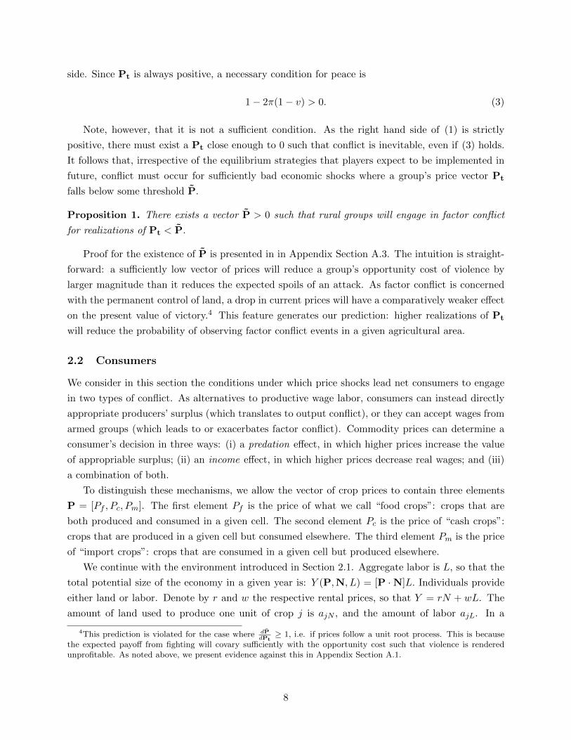
side. Since Pt is always positive, a necessary condition for peace is

1− 2π(1− v) > 0. (3)

Note, however, that it is not a sufficient condition. As the right hand side of (1) is strictly

positive, there must exist a Pt close enough to 0 such that conflict is inevitable, even if (3) holds.

It follows that, irrespective of the equilibrium strategies that players expect to be implemented in

future, conflict must occur for sufficiently bad economic shocks where a group’s price vector Pt

falls below some threshold P.

Proposition 1. There exists a vector P > 0 such that rural groups will engage in factor conflict

for realizations of Pt < P.

Proof for the existence of P is presented in in Appendix Section A.3. The intuition is straight-

forward: a sufficiently low vector of prices will reduce a group’s opportunity cost of violence by

larger magnitude than it reduces the expected spoils of an attack. As factor conflict is concerned

with the permanent control of land, a drop in current prices will have a comparatively weaker effect

on the present value of victory.4 This feature generates our prediction: higher realizations of Pt

will reduce the probability of observing factor conflict events in a given agricultural area.

2.2 Consumers

We consider in this section the conditions under which price shocks lead net consumers to engage

in two types of conflict. As alternatives to productive wage labor, consumers can instead directly

appropriate producers’ surplus (which translates to output conflict), or they can accept wages from

armed groups (which leads to or exacerbates factor conflict). Commodity prices can determine a

consumer’s decision in three ways: (i) a predation effect, in which higher prices increase the value

of appropriable surplus; (ii) an income effect, in which higher prices decrease real wages; and (iii)

a combination of both.

To distinguish these mechanisms, we allow the vector of crop prices to contain three elements

P = [Pf , Pc, Pm]. The first element Pf is the price of what we call “food crops”: crops that are

both produced and consumed in a given cell. The second element Pc is the price of “cash crops”:

crops that are produced in a given cell but consumed elsewhere. The third element Pm is the price

of “import crops”: crops that are consumed in a given cell but produced elsewhere.

We continue with the environment introduced in Section 2.1. Aggregate labor is L, so that the

total potential size of the economy in a given year is: Y (P,N, L) = [P ·N]L. Individuals provide

either land or labor. Denote by r and w the respective rental prices, so that Y = rN + wL. The

amount of land used to produce one unit of crop j is ajN , and the amount of labor ajL. In a

4This prediction is violated for the case where dPdPt≥ 1, i.e. if prices follow a unit root process. This is because

the expected payoff from fighting will covary sufficiently with the opportunity cost such that violence is renderedunprofitable. As noted above, we present evidence against this in Appendix Section A.1.

8

competitive equilibrium, farms earn zero profits:

rajN + wajL = Pj , (4)

where Pj is the internationally determined price of one unit. Net consumers u maximize consump-

tion. Indirect utility is therefore a function of prices and wages: Vu(P, w).

The first key addition to this environment is the existence of an appropriation sector for con-

sumers: property rights are sufficiently weak to enable net consumers (or groups of net consumers)

to appropriate surplus from landowners through the technology of output conflict. This can be

chosen as an alternative to productive wage labor, as in Dal Bo and Dal Bo (2011). Denote by

LQ the share of labor in the appropriation sector, and by Q(LQ) the fraction of total output that

is redistributed from the productive sector to the appropriation sector, where the function Q(LQ)

is positive, continuous and strictly concave due to congestion effects, so that Q(L) < 1. The total

amount of appropriated production is therefore Q(LQ)[P ·N](L− LQ). A net consumer’s decision

to appropriate is one that satisfies the following condition:

Q(LQ)[P ·N](L− LQ)

LQ> [1−Q(LQ)]w, (5)

where the left hand side represents the individual payoff from appropriation, given by the value

of appropriated goods per unit of labor allocated to that sector, and right hand side is the payoff

from one of unit of productive work net of appropriation.

Net consumers will appropriate rather than work productively as long as it is profitable to do

so. Denoting by A the left hand side of (5), and by W the right hand side, the equilibrium level

of appropriation will be reached when A = W. Our goal is to determine how shocks to Pf , Pc,

and Pm will affect this equilibrium. If dAdPj− dW

dPj> 0, then the equilibrium level of output conflict

Q(LQ) will increase.

In Appendix A.4, we derive how changes in prices for food crops, cash crops, and import crops

affect conflict. We summarize these results here.

1. First, in food-producing cells, higher food prices Pf will increase the incidence of output

conflict in the short run. The intuition is straightforward: higher food prices increase the value

of output that accrues to landowners (generating a predation effect), while simultaneously

decreasing the real wage of laborers in the short run (generating an income effect). This

combination of effects increases the profitability of output conflict relative to productive

wage labor (Proposition 2 ).

2. Second, the effect of cash-crop prices Pc on equilibrium output conflict is lower than the effect

of food-crop prices Pf on equilibrium output conflict. This is because increases in Pc and Pf

both increase the value of appropriable surplus, generating a predation effect, but only Pf

will reduce real wages through an income effect (Proposition 3 ).

3. Finally, in consumer cells, higher imported food crops Pm will increase both output conflict

9

and factor conflict. In this case, Pm generates an income effect only. In keeping with a

broad literature showing that poor households undertake costly or risky behaviors in response

to income shocks that they cannot otherwise smooth (de Janvry et al., 2006; Dupas and

Robinson, 2012; Miguel, 2005), this will increase the likelihood that poor consumers will (i)

supply labor to local armed groups, which facilitates more factor conflict battles (Observation

1 ); and (ii) engage in output conflict, where output can be construed in a general sense as

appropriable property of positive value (Observation 2 ).

2.3 Summary

Table 1 summarizes the main theoretical predictions.5

Table 1: Theoretical predictions

Factor conflict Output conflict

Food-producing cells dConflictdPf

< 0 dConflictdPf

> 0

Food-consuming cells dConflictdPm

> 0 dConflictdPm

> 0

In food-producing cells, higher food prices will reduce factor conflict, as rural groups choose to

farm rather than to attack neighboring territory. At the same time, higher food prices will also

increase output conflict, as net consumers appropriate increasingly valuable surplus while their real

wages fall.

In food-consuming cells, higher prices reduce real wages. Consumers at the margin of a target

consumption level are therefore more likely to accept a living wage from armed groups in conflict

zones (which translates to more factor conflict); and to engage in interpersonal crime or looting

(which translates to more output conflict).

3 Data and measurement

3.1 Structure

We construct a panel grid dataset to form the basis of our main empirical analysis, consisting

of 10,229 arbitrarily drawn 0.5 X 0.5 decimal degree cells (around 55km × 55km at the equator)

covering the continent of Africa. The unit of analysis is the cell-year. The cell resolution is presented

graphically in Appendix Figure A1.

5We omit the distinction between food crops and cash crops for simplicity. We also do not consider the prospectof producers engaging in output conflict, as the opportunity cost of doing so is equal to the value of output thatwould be contested.

10

3.2 Conflict

Main factor conflict measure: UCDP Factor Conflict Theory dictates that the measure

of factor conflict must capture large-scale conflict battles associated with the permanent control of

territory, as distinct from transitory appropriation of food.6 The Uppsala Conflict Data Program

(UCDP hereafter) Georeferenced Event Dataset project is particularly suitable. It represents a spa-

tially disaggregated edition of the well-known UCDP country-level conflict dataset used frequently

in the literature. It records events involving “the use of armed force by an organised actor against

another organised actor, or against civilians, resulting in at least 1 direct death” (Sundberg and

Melander, 2013, pp.4). Moreover, it includes only dyads that have crossed a 25-death threshold

in a single year of the 1989-2010 series.7 The data are recorded from a combination of sources,

including local and national media, agencies, NGOs and international organizations. A two-stage

coding process is adopted, in which two coders use a separate set of procedures at different times

to ensure that inconsistencies are reconciled and the data are reliable. Conflict events are coded for

the most part with precision at the location-day level. We aggregate to the cell-year level, coding

the variable as a one if any conflict event took place, and zero otherwise. This reduces the potential

for measurement error to bias results, and is in line with the literature.8

Summary statistics for this measure of conflict incidence are presented in the top panel of

Table 2. The unconditional probability of observing a factor conflict event in a cell-year is 2.7%,

while the standard deviation is relatively large at 0.162. The row immediately beneath displays the

corresponding onset statistics, defined as I(Conflictit = 1 | Conflictit−1 = 0), where i is a cell.

This sample contains all zeros plus onset years only. Conditional on peace at t− 1, conflicts occur

with probability of 1.4%. Beneath this again are offset statistics, defined as I(Conflictit+1 =

0 | Conflictit = 1). This is the equivalent of measuring the additive inverse of the persistence

probability. Conditional on conflict in a given cell-year, the probability of peace the following

year is 53.5%. Hence, this sample consists of all conflict years only. The sample average also

indicates that time dependence is unlikely to be a first order concern in the analysis, given that a

(thin) majority of conflict events are followed by peace. Nevertheless, we model onset and offset

separately in the formal analysis, in part as a means of assuaging concerns of autocorrelation, and

in part due to our theory. (In robustness tests, we also operate an alternative measure of factor

conflict from the ACLED dataset; see Appendix B.2).

Main output conflict measure: ACLED Output Conflict Following our theory, the output

conflict measure must capture violence over the appropriation of surplus. These events are likely

6In fact, this definition can be relaxed: our measure of factor conflict need only capture battles in which thecontested resource is not food.

7For example, battles between the UNRF II and the Ugandan government crossed the 25-death threshold in 1997,therefore events in 1996 and 1998 in which deaths d were 0 < d < 25 are also included.

8For each event, UCDP records the headline of the associated news article. Examples include: “Five said killed,250 houses torched in clashes over land in central DRC.” BBC Monitoring Africa, 9/21/2007; “Tension runs high inwest Ivory Coast cocoa belt. [20 killed.]” Reuters, 11/14/2002; “Tribes in Chad feud over land around well, 50 dead.”Reuters, 11/23/2000.

11

to be more transitory and less organized than large-scale factor conflict battles over the permanent

control of territory. For this, the Armed Conflict Location and Event Data (ACLED) project

provides an appropriate measure, covering the period 1997-2013. Like the UCDP project, ACLED

records geocoded conflict events from a range of media and agency sources. Of eight conflict event

categories included in the data, we discard all of the organized group “battle” categories and are

left with two remaining forms of violence: “riots and protests” and “violence against civilians”.

We allow the output incidence measure to equal 1 if any of these two events occur in a cell-year,

and 0 otherwise. Each classification includes unorganized violence by any form of group, including

unnamed mobs. This definition captures incidences of food riots, farm raids and crop theft, as well

as more general rioting and looting. No fatalities are necessary for events to be included in the

data. Unconditional output conflict probability is 5%.9

Micro-level output conflict from Afrobarometer We turn to the Afrobarometer survey se-

ries for micro-level measures of interpersonal output violence. The first four rounds yield over

65,000 responses across 19 countries to questions on whether or not individuals experience theft or

violence in the preceding year. In our formal analysis, we replace years with biannual time periods

in order to increase our temporal variation. This produces 13 periods from 1999 to 2009. The data

are collected as repeated cross-sections. In Table 2, we see that over 30% of respondents report

having experienced theft in the past year, while 13% have been victims of violence.10 In validation

tests (discussed in Appendix Section C.4), we show that the ACLED output conflict variable is

significantly correlated with both Afrobarometer survey measures, while the UCDP factor conflict

variable is correlated with neither. The Afrobarometer dataset also permits us to investigate the

first stage relationship between prices and poverty.

The upper panel of Figure 2 displays a time plot of the two main cell-level conflict event vari-

ables. On the vertical axis is the count of cells in which at least one conflict event occurs. UCDP

Factor Conflict runs from 1989 to 2010, and ACLED Output Conflict runs from 1997 to 2013. Note

that output conflict does not appear to vary with factor conflict, and is at no stage less frequent.

9ACLED data observations are accompanied by a brief note on the nature of each event. The output conflict eventscontain 3438 mentions of “riot-” (i.e., including “rioters”, “rioting”, and so on), or 0.39 for each time our outputconflict incidence variable takes a value of 1; 1302 mentions of “raid-” (0.15); 1083 mentions of “loot-” (0.12); 1173mentions of “thief”, ”thieve-”, “theft”, “steal-”, ”stole-”, “crime”, “criminal” or “bandit” (0.13); and 383 mentionsof “food” (0.04). Examples of specific notes are: “Around 25 MT of assorted food commodities to be distributed by aLNGO were looted from its storage facility in Bacad Weyne in the night of 31/07/2011.” (Somalia); “A dozen armedmen looted and pillaged food stocks in Boguila. After shooting their weapons in the air and attacking food stores, thebandits vanished within 45 minutes”. (Central African Republic)

10The respective questions are: ”Over the past year, how often (if ever) have you or anyone in your family: Hadsomething stolen from your house?” and ”Over the past year, how often (if ever) have you or anyone in your family:Been physically attacked?”

12

3.3 Prices

To study the causal effect of price variation on conflict, we require price data with at least three

general properties: variation over time; variation that is not endogenous to local conflict events

and/or determined by local factors that might jointly affect prices and conflict; and variation

that significantly affects real income at the household level in opposing directions across producers

and consumers. Our approach is to construct local price series that combine plausibly exogenous

temporal variation in global crop prices with local-level spatial variation in crop production and

consumption patterns.

The middle and lower panels of Figure 2 present sets of global crop price series covering 1989

to 2013, our period of analysis. The prices are taken from the IMF International Finance Statis-

tics series and the World Bank Global Economic Monitor (described in more detail in Appendix

Section B.1). The top panel displays three important staple food crops for African consumers and

producers: maize, wheat and rice, with prices in the year 2000 set to an index value of 100. Immedi-

ately apparent are sharp spikes in 1996 and, more notably, 2008 and 2011. Only wheat falls short of

an index value of 300 in this period. In the lower panel, we present a selection of three non-staples

(“cash crops” henceforth): coffee, cocoa and tobacco. These exhibit more heterogeneity, though

coffee and cocoa prices reach high points toward the end of the series, before falling through 2012

and 2013. For both sets of crops, our study period captures historically important variation.

Variation in global crop prices is plausibly exogenous to local conflict events in Africa. As

our sample consists of African countries only, we avoid serious concerns that cell-level conflict

events directly affect world food prices—the entire continent of Africa accounts for only 5.9% of

global cereal production over our sample period. Nevertheless, other factors could affect both

simultaneously. The World Bank (2014) posits a range of likely explanations for food price spikes

in 2008-09 and 2010-11. For instance, the surge in wheat prices is attributed to weather shocks

in supplier countries like Australia and China, while the concurrent maize price shock is jointly

explained by rising demand for ethanol biofuels and high fructose corn syrup, as well the effect of

La Nina weather patterns on supply in Latin America. Although this set of correlates is broad,

they are unlikely to influence our conflict measures through the same confluence of spatial and

temporal variation as our price indices. For example, it is unlikely that a dry spell in Argentina

could influence concurrently violence in rural and urban Uganda in opposing directions, other than

through an effect on world food prices. Notwithstanding this, we variously control for country-year

fixed effects, country time-trends, weather conditions, and oil prices in our formal analysis.

Finally, several studies evaluate large impacts of food price shocks on household welfare and

consumption in developing countries. For example, Alem and Soderbom (2012) show that a 92%

food price increase in Ethiopia between 2007 and 2008 significantly reduced consumption in poor

urban households. Using survey data from 18 African countries in 2005 and 2008, Verpoorten et al.

(2013) find that higher international food prices are simultaneously associated with lower and higher

consumption in urban and rural households respectively. This resonates with our own analysis in

the Appendix Section C.4, where we use Afrobarometer survey data to identify opposing effects of

13

higher consumer and producer prices on self-reported poverty indices. Ivanic et al. (2012) focus

on the 2010-11 spike, evaluating the effect of price changes for 38 commodities on extreme poverty

in 28 countries. They find that the shock pulled 68 million net consumers below the World Bank

poverty line of $1.25, while 24 million were pushed out of poverty through the producer mechanism.

Producer Price Index To compute producer prices, we combine temporal variation in world

prices with rich high-resolution spatial variation in crop-specific agricultural land cover circa 2000.

The spatial data come from the M3-Cropland project, described in detail by Ramankutty et al.

(2008). The authors develop a global dataset of croplands by combining two different satellite-

based datasets with detailed agricultural inventory data to train a land cover classification dataset.

The method produces spatial detail at the 5 min level (around 10km at the equator), which we

aggregate to our 0.5 degree cell level. Table 2 displays summary statistics on cropland coverage:

63% of cells contain cropland area larger than zero, while cropland as a share of the total area of

the continent is 7.2%. Figure 3 presents crop-specific maps for a selection of six major commodities

(maize, rice, wheat, sorghum, cocoa and coffee).

Our producer price index is the dot product of a vector of crop-specific cell area shares and the

corresponding vector of global crop prices, with each crop weighted by the extent to which it is

traded internationally by the country in which the cell falls. For cell i, country c and year t the

price index is given by

PPIict =

n∑j=1

(Pjt ×mjc + xjc

yjc︸ ︷︷ ︸trade weight

× Njic︸︷︷︸crop land share

) (6)

where crops j . . . n are contained in a set of 11 major traded crops that feature in the M3-Cropland

dataset and for which international prices exist. Trade weights are defined as the sum of imports

and exports divided by total domestic production for a given crop, averaged over our entire sample

period and Winsorized to form a time invariant weight varying from 0 to 1.11 Inclusion of these

weights ensures that our cell-specific index is not affected by variation in world prices of crops that

are neither imported nor exported. Global crop-specific prices taken from the IMF International

Finance Statistics series and the World Bank Global Economic Monitor and indexed at 100 in the

year 2000.12 In addition to this aggregated index, we also compute disaggregated variants that

measure only food crop prices Pf (those which constitute more than 1% of calorie consumption in

the entire sample) and cash crops Pc (the rest). The index varies over time only due to plausibly

exogenous international price changes; all other components are fixed.

Consumer Price Index The consumer price index we construct is similar in structure to the

producer price index, only the spatial variation instead comes from country-level data on food

11Trade and production statistics are taken from the FAO Statistics Division, accessible at http://faostat3.fao.org/home/E as at August 30th, 2015.

12Appendix Section B.1 presents the the descriptions and sources for the price data in more detail.

14

consumption from the FAO Food Balance Sheets. Food consumption is calculated as the calories

per person per day available for human consumption for each primary commodity. It is obtained by

combining statistics on imports, exports and production, and corrected for quantities fed to livestock

and used for seed, and for estimated losses during storage and transportation. Processed foods are

standardized to their primary commodity equivalent. Although the procedure is harmonized by

the FAO, gaps in quality are still likely to emerge across countries and over time. Partly for this

reason, we construct time-invariant consumption shares based on averages over the series 1985-

2013.13 These are similar to the crop shares Njic above, only that crop shares in this instance

represent calories consumed of crop j as a share of total calories consumed per person in a given

country over the series.

Formally, the consumer price index in cell i, country c and year t is given by:

CPIct =

n∑j=1

(Pjt ×mjc + xjc

yjc︸ ︷︷ ︸trade weight

× θjc︸︷︷︸crop calorie share

) (7)

where crops j . . . n are contained in a set of 18 crops that are consumed in Africa and for which

world prices exist, making up 56% of calorie consumption in the sample, and containing important

staples such as maize, wheat, rice and sorghum, as well as sugar and oil palm, which are used to

process other foods. Again, temporal variation comes only from the price component.

3.4 Other data

In Table 2, Urban area % is share of each cell area that is classified as urban by the SEDAC

project at Columbia University. The same source provides data on Population (estimated for the

year 2000) and Distance to city (measured in 1000s of km).14 Luminosity is a dummy variable

indicating whether or not light density within cells is visible from satellite images taken at night

during 2007 and 2008. These data are increasingly used as measures of subnational economic

development, given the relative dearth of quality data in less developed regions, and in particular

those affected by civil conflict (see Michalopoulos and Papaioannou, 2013, for a discussion on the

particular suitability of nighttime lights as measure for economic development in Africa).15

Finally, Appendix Figure A2 plots the FAO Global Food Price Index (the most widely used

index of its type) from 1990 to 2014. Spikes in 1996, 2008 and 2011 are consistent with the raw

price data introduced above.

13Incorporating data from 1985 onwards allows for lags in the formal analysis.14SEDAC datasets are downloadable at: http://sedac.ciesin.columbia.edu/data/sets/browse. Accessed Au-

gust 10th, 2015.15Under the assumption that luminosity measures economic development with a lag, we look to measure it at a

relatively late stage in our series, being careful to avoid the period from 2010 onward due to the peaks in conflictobserved in the ACLED dataset. We opt for a time invariant measure based on imagery from 2007 and 2008. Theoriginal data come from the Defense Meteorological Satellite Program’s Operational Linescan System that reportsimages of the earth at night captured from 20:30 to 22:00 local time. We take our sample from Michalopoulos andPapaioannou (2013).

15

4 Estimation framework

The standard empirical approach to estimating the impact of income shocks on conflict takes some

variation of the form:

conflictct = αc + βnPt + γc × trendt + εct (8)

where the outcome is an indicator for conflict incidence in country c and year t; αc captures

country fixed effects, accounting for all time-invariant country characteristics that explain civil

conflict; γc × trendt is a country-specific linear time trend included to capture all time-varying

factors that exhibit an analogous trend to conflict in country c; and εct is the disturbance term,

which is allowed to be serially correlated at the country level. The Pt term on the right hand side

represents an exogenous income shock variable. In the case of food prices, that could take the form

of the FAO world food price index, as in Hendrix and Haggard (2015) in their analysis of urban

unrest, or could be a climate-related income shock, as in Miguel et al. (2004).

As noted above, this approach fails to account for potential opposing effects of prices on produc-

ers and consumers within a given country, likely leading to attenuated estimates of βn. Furthermore,

it makes it difficult to distinguish between the opportunity cost and state capacity mechanisms as

structural explanations for any significant result. To overcome these barriers to inference, we in-

stead require an empirical model that explicitly accounts for the opposing effects of world food

prices on producers’ and consumers’ real wages.16

Factor conflict To study factor conflict, we propose a cell-level variant of equation (8), replacing

the general price term with the producer and consumer price indices as follows:

factor conflictict = αi +

2∑k=0

βpt−kPPIict−k +

2∑k=0

βct−kCPIct−k + γc × trendt + εict (9)

where the outcome is factor conflict in cell i measured as incidence, onset or offset binary variables;

αi represents cell fixed effects; PPI is the producer price index; CPI is the consumer price index;

the fourth term is the country-specific time trend; and the final term is the error, which we cluster

along two dimensions to allow for serial correlation at the cell-level and spatial correlation across

cells within a country.17 We sum price effects over three years to account for delayed effects of

past shocks, or potentially for displacement effects where shock hasten conflict that would have

happened anyway.18 We estimate the specification with both a linear probability model (LPM)

as well as conditional logit, preferring LPM for the main analysis as it allows for more flexible

specifications and a clear interpretation of the coefficients; results are qualitatively similar either

way. In line with our theoretical predictions, when the outcome is factor conflict incidence or onset

we expect that βp will be negative, and βc will be positive. When the outcome is factor conflict

16We explore the quantitative implications of this “naive” approach in Section 5.4 below.17We also present results where the error term is allowed to be spatially and serially correlated in groups of

contiguous cells, following Conley (1999)18Results are not sensitive to the choice of k = {0, 1, 2}.

16

offset, we expect the opposite.

The identifying assumption in Equation 9 is that, after accounting for time-invariant factors

at the cell level and common trending factors at the country level, variation in consumer and

producer prices are not correlated with other unobserved factors that also affect conflict. One

potential concern is that unobserved shocks that are not picked up by the country trends could

be correlated with both crop prices and conflict. To account for this, we control for some of these

potential confounds (such as local weather and oil price indices) in robustness tests, and we also

estimate an alternate form of Equation 9 that includes country-year fixed effects γct:

factor conflictict = αi +2∑

k=0

βpt−kPPIict−k + γct + εict (10)

Here, βp is estimated off within-country-year variation in prices and conflict, eliminating concern

about common time shocks. The cost to this approach is that we can no longer include consumer

prices, as these do not vary within-country in a given year.19

Output conflict For output conflict, our theory predicts (i) that rising food prices will increase

incidence in food-producing cells, in contrast to case of factor conflict; (ii) that this effect will be

larger for food crop price shocks than for cash crop price shocks; and (iii) that increases in the

prices of imported food crops will lead to more output conflict. We test these predictions with the

following specifications:

output conflictict = αoi +2∑

k=0

βpft−kPPIfoodict−k +

2∑k=0

βpct−kPPIcashict−k

+

2∑k=0

βmt−kCPIct−k + γc × trendt + eict (11)

and

output conflictict = αoi +

2∑k=0

βpft−kPPIfoodict−k +

2∑k=0

βpct−kPPIcashict−k + γct + eict, (12)

where PPIfood is a component of the producer price index that contains information only on food

commodities that constitute more than 1% of total average consumption in our sample (capturing

Pf from the theoretical model). These include the major staples of maize, wheat, rice and sorghum.

The PPIcash component picks up the remaining cash crops such as coffee, tea and tobacco (cap-

turing Pc from the model). Equation (11) includes the consumer index CPI to capture the impact

of prices net of the production effects (Pm in the model). Equation (12) includes country-year fixed

effects, leaving only the two subnational producer price indices. According to the model, βpf and

19In later specifications, we use our theory to introduce heterogeneity across cells that permits the inclusion of boththe consumer price index and country-year fixed effects.

17

βm will be positive, and βpf > βpc.20

5 Results

5.1 Factor conflict

Main results In all regressions, price indices are measured in terms of the average within-cell

(i.e., temporal) standard deviation. Panel A in Table 3 presents results from regressions that omit

the consumer price index and include country × year fixed effects. The producer price index used in

column (1) omits trade weights, and the sample therefore includes cells from countries that do not

feature in the FAO dataset. Column (2) includes trade weights in the index. These specifications

are repeated for conflict onset and offset in the following columns in order to decompose the conflict

incidence effects in (1) and (2). In both incidence specifications, higher producer prices significantly

reduce the risk of factor conflict. The magnitudes are large: a one (within-cell) standard deviation

rise in producer prices lowers the probability of factor conflict by 15.4% of the mean without trade

weights, and by 17.7% of the mean with trade weights. Both estimates are significant at the 1%

level with Conley standard errors. When errors are (two-way) clustered, the trade-weight estimate

is significant at the 5% level and the without-trade-weight estimate is significant at the 1% level.

Both estimates are driven jointly by a lower onset risk and by a higher offset probability (i.e. a

reduction in conflict duration).

Panel B in Table 3 presents the main results that include the consumer price index. Three facts

are particularly noteworthy. First, higher consumer prices significantly increase the duration of

factor conflict. A standard deviation rise in prices reduces the probability of a conflict ceasing by

16.5% and 13.7% with and without trade weights respectively, but the effect on conflict onset is not

significant.21 This is consistent with the idea that rising prices force low-income net consumers to

join existing armed groups rather than launch new conflicts. Second, the magnitude of the producer

effects is larger across the board than in Panel A. This is consistent with the idea that the latter

estimates are biased downward due to omitted variable bias. Third, producer and consumer price

effects are significantly different from each other in all six specifications. This is consistent with

our main model prediction on factor conflict.

In Appendix Section C.1, we explore rthe obustness of these main results to the inclusion of

weather and oil price controls, to alternate ACLED-based measures of territorial change, to different

levels of aggregation, to explicitly modeling spatial spillovers, and to a conditional logit rather than

a linear probability model estimator. Our main results are robust to all of these variants.

The upper panel of Figure 4 presents visual output based on a variant of the specification

estimated in column (1). The regression includes quadratic fits of the producer and the consumer

price indices (without lags), as well as cell fixed effects and country-year time trends. The figure

20The predictions are with respect to conflict incidence and onset; the opposite sign is predicted when conflict offsetis the outcome variable.

21Unless otherwise stated, results presented hereafter are based on models with trade weights in the price indices.

18

support a linear treatment of the main effects.

Heterogeneity Our model also provides guidance on a source of heterogeneity in the consumer

price effect that we can test in the data. We outline conditions necessary for high food prices to

cause net consumers to join armed conflict groups: they must have few assets for dissaving; they

must have no access to credit or insurance; and they must be earning a lower wage than that offered

by the armed conflict group. In short, we should not expect to find the same impact of consumer

prices on factor conflict in more economically developed cells, all else equal.

Following a now-voluminous literature, we proxy local economic development by using satellite-

based measures of luminosity at night, coding a luminosity variable equal to unity if a grid cell

showed non-zero luminosity in 2007-08. The impact of the consumer price index on factor conflict

is therefore predicted to be lower in cells where luminosity = 1. It is conceivable also that in the

event of negative price shocks, farmers who are proximate to local non-agricultural labor markets

will be less likely to join armed groups than those who do not. If we assume that lit cells are more

likely than dark cells to contain employment opportunities outside of the agricultural sector (all

else equal), then the impact of the producer price index on factor conflict also ought to be closer

to zero where luminosity = 1.

Introducing the luminosity variable allows us to estimate a variant of equation 10 that contains

CPIct−k×luminosityic, PPIict−k×luminosityic and country × year fixed effects, as the interaction

generates variation in the consumer price index at the subnational level. To that end, this exercise

serves as both a robustness exercise as well as a test of theoretical implications.

We are cautious of several factors that may impede our interpretation of these interaction effects.

First, the interaction variable might simply capture the fact that lit cells are likely to contain larger

populations, which is necessary for conflict to occur in the first place. We thus control for cell-

year level CPI and PPI × population interactions in all specifications.22 Second, global price

pass-through is likely to be larger in lit cells than in dark ones, even controlling for population,

as economic development may reflect more trade openness. This would bias the effect of the

luminosity interaction terms towards zero, as we are predicting that economic development mutes

the effect of prices on violence (while the passthrough story implies the opposite). We attempt to

capture this by creating a proxy for market remoteness, measured by the distance in 1000kms to

the (next) nearest lit cell. Third, the luminosity variable is correlated with other factors that might

be associated with conflict through alternative mechanisms. We consider three: distance to capital

city, which captures the possibility that state counterinsurgency capacity is weaker the farther

one is from the capital; mountain terrain, with may facilitate insurgency; and the sophistication of

precolonial governance in the ethnic homeland containing a given cell, measured by Murdock (1957)

as the degree of political centralization, and found by Michalopoulos and Papaioannou (2013) to

22We compute the cell-level population variable using data from the Socioeconomic Data and Applications Center(SEDAC) project at Columbia University. Datasets are downloadable at: http://sedac.ciesin.columbia.edu/

data/sets/browse.

19

be correlated strongly with contemporary economic development.23

The results of this test are presented in Table 4. Column (1) features a model with country

time trends, cell fixed effects, and prices × population as controls; in column (2) we add country

× year fixed effects; and in column (3) we add the rich battery of controls described above. Con-

flict incidence is the dependent variable In all three specifications. The main finding is that, in

specifications with country × year fixed effects, a one standard deviation rise in consumer prices

significantly increases factor conflict in dark cells by 19-20% compared to more economically devel-

oped lit cells. We also note substantial heterogeneity in the impact of the PPI—from −48% in dark

cells to −20.8% in lit cells in column (3)—but these estimates are narrowly outside of conventional

levels of statistical significance.

Taken together, this exercise supports an implication of theoretical model: that the effect of

consumer price shocks on factor conflict is weaker in more economically developed areas. We also

find suggestive evidence that lower producer prices are less likely to spark conflict when farmers

have recourse to proximate non-agricultural labor markets. Both forms of heterogeneity are proxied

by nighttime luminosity from satellite images. This finding suggests that is it not only economic

shocks that relate to conflict, but also the interaction of shocks and levels.

5.2 Output conflict: ACLED

Main results In Table 5, we present the impact of the aggregated PPI and the CPI on output

conflict to allow for a comparison with the factor conflict results. Columns (1) and (2) display

results from specifications with country × year fixed effects (CYFE) and without the CPI. In

contrast to the case of factor conflict, we see that a one standard deviation rise in producer prices

leads to an increase in the probability of output conflict of 14.4% and 15.1% with and without

trade weights respectively. In (3) and (4), the impact of the CPI is 14.4% and 8.0%. All estimates

are significant at the 1% level.

The lower panel of Figure 4 presents visual results from a regression of output conflict on the

producer price index, the consumer price index (both quadratic fits), a country time trend and

cell fixed effects. In contrast to the upper panel, the producer price effect slopes upward. Taken

together, the two panels corroborate the predictions outlined in Table 1.

Table 6 and Appendix Table A8 present results from the specifications described in Section 4,

in which the producer price index is separated into food crops (Producer Price Index: Food Crops)

and cash crops (Producer Price Index: Cash Crops). Six models are featured: one without trade

weights and one with trade weights for each of the output conflict incidence, onset and onset

outcome. Higher food prices lead to a significant and economically large increase in output conflict

incidence and onset, whether with Conley standard errors or with errors clustered by cell and by

country-year. Focusing on column (2) in Table 6, a standard deviation increase in food prices raises

the probability of output conflict incidence by 16.6%. By contrast, cash crop prices have no clear

23Data on distance to capital city and mountain terrain are taken from the PRIO GRID dataset; data on pre-colonialpolitical centralization is taken from Michalopoulos and Papaioannou (2013).

20

impact. Consistent with our predictions, both effects are significantly different from each other

at the 1% level in all incidence and onset regressions, although this is not the case in the offset

regressions, where both effect are close to zero. Again in line with our theory, the consumer price

index also enters with a large and significant coefficient: a standard deviation rise leads to a 7.9%

increase in output conflict incidence, and analogous results are shown for onset and offset.

In Appendix Table A8, we omit the consumer price index and include country × year fixed

effects, finding similar results.24 As in case of factor conflict above, we test for robustness to the

inclusion of potential weather and oil confounds, to higher levels of aggregation, and to alternate

estimators, and find our results quantitatively and qualitatively robust in each case (see Appendix

C.2).

We also explore whether our measure of output conflict is just picking up “food riots” that

may be driven as much by a desire to provoke government policy changes than by a desire to

directly appropriate property from others (Bellemare, 2015). This interpretation is supported by

Hendrix and Haggard (2015) and Bates and Carter (2012), who find that governments frequently

alter policies in favor of consumers in the wake of price shocks. Food riots in this context will

occur in urban centers where government authorities can be expected plausibly to respond, and we

therefore interact our consumer price index with two different measures of urbanization in order to

detect whether results are differentially driven by urban unrest.

Results are shown in Table A13 and described in more detail in Appendix C.2. Using either

an area-based or population-based definition of whether a cell is “urban”, we find that the effect

of higher CPI on output conflict remains positive and significant in non-urban areas. The effect in

urban areas is larger than the rural effect using the area-based measure, but is indistinguishable

using the population-based measure. We conclude that our main output conflict results are not

driven by urban food riots or protests designed to create unrest and agitate for policy reforms.

We also investigate whether the contrasting impact of producer food crop prices on both out-

comes can be fully explained by the different sample periods or data collection projects. Results

suggest that this is not the case, with findings qualitatively unchanged on the sample restricted to

the same set of years (see Appendix Table A14).

5.3 Output conflict: Afrobarometer

In this section, we incorporate data on interpersonal conflict from multiple rounds of the Afro-

barometer household survey project. Merging our high resolution panel grid with Afrobarometer

permits an alternative strategy to investigate the relationship between food prices and output con-

flict, as well as a direct way to assess the assumed “first stage” relationship between food price

movements and income movements, as assumed in our theory. We describe how we process and

merge the Afrobarometer data in Appendix Section C.4.

In Table A15, we examine the effect of the producer and consumer price indices on three different

24The results in Appendix Table A8 also show that Conley standard errors are smaller than two-way clusterederrors, which are presented in the main text.

21

self-reported poverty measures, controlling for survey round fixed effects, country fixed effects, a

country-specific time trend, the age of the respondent, age squared, education level, gender, urban

or rural primary sampling unit, and a vector of 0.5 degree cell-level crop-specific land area shares,

so that the producer price index is not picking up time-invariant features of agricultural production.

We find that a one standard deviation increase in the CPI raises the probability that a respondent

is above the median poverty index value by 12.2%, or from 45% to 50.5% at the mean. We see

that an equivalent change in the PPI has a negligible effect on the overall poverty index using

the full sample, but that higher producer prices are associated with lower self-reported poverty

for respondents who report farming as their primary source of income. These results are broadly

consistent with the assumptions of our theory: higher food prices represent negative income shocks

for consumers, and positive shocks for producers.

We also confirm that our Afrobarometer measures of interpersonal conflict—which include

whether individuals over the previous year report (i) having been victims of theft; (ii) having

been victims of physical assault; (iii) or having partaken in “protest marches” (which includes

demonstrations, riots or looting)—are more likely picking up output conflict rather than factor

conflict. We regress each binary indictor on our cell-level ACLED Output Conflict variable in three

specifications: one bivariate, one with survey round fixed effects and country fixed effects, and

one that adds the UCDP Factor Conflict measure in order to determine if the survey measures

are also (or instead) capturing factor conflict. In eight of the nine specifications, the survey mea-

sures correlate significantly with ACLED Output Conflict Variable. The exception is the bivariate

protest variable regression. The UCDP Factor Conflict variable does not enter significantly in any

specification.

Food prices and output conflict in Afrobarometer Proposition 2 implies that higher food

prices will cause net consumers to appropriate output in food-producing areas. From whom do

they appropriate? In the model, we imply that output violence is perpetrated against landowners.

In the data, we can approximate this by identifying commercial farmers, who number 6,751 (11%)

of the 59,871 respondents to the question on occupation. Moreover, we can also include traders

(7%) as potential victims of output violence, relaxing the assumption that output is traded only

by producers at the farm gate. We focus specifically on the theft and violence outcomes, as they

most directly correspond to the theoretical concept of output violence.

The main disadvantage of the micro-level Afrobarometer data is that we do not observe the

same farmers in different periods, meaning we cannot control for individual unit fixed effects as in

the cell-level analysis. This raises the possibility that unobserved individual factors may explain

why commercial farmers respond differently to price shocks than do other survey respondents. To

overcome this problem, we compare whether the impact of higher prices on reported conflict among

farmers/traders is higher in food-producing cells than in cash-crop-producing cells. According to

our model, output conflict rises in the PPI for food crops because the value of appropriable output

increases while real wages simultaneously decline. By contrast, the PPI for cash crops will raise the

22

value of appropriable output without causing a simultaneous decline in real wages. We can estimate

the difference in these effects with a framework similar in concept to a triple difference approach.

Two specifications are estimated for each of the theft and violence outcomes. In the first, we

control for country fixed effects and for crop-specific cell area shares in order to account for fixed

differences between areas that grow different crops.25 We also control for occupation, and for the

set of controls listed in the previous subsection, including a country-specific time trend and fixed

effects for countries and survey rounds. In the second specification, we control for cell fixed effects—

therefore holding all cell-level time-invariant characteristics fixed—as well as country × period fixed

effects and the individual controls. That allows us to compare only the effect of price changes on

farmers/traders between food-producing cells and cash crop producing cells within countries.

Table 7 shows our main results. In column (1), we present the country fixed effects model with

theft as the outcome. We first note that traders are significantly more likely than other respondents

to be victims of theft when food prices rise in food-producing cells. By contrast, farmers and traders

are both less likely to be victims of theft when cash crop prices rise in cash-crop-producing cells.

Finally, the consumer price index also enters with a positive (but noisy) coefficient, indicating that

food prices increase theft across the full sample (i.e., in cells where food is imported). The second

panel presents treatment effects, standard errors and the associated p-values for the impact of food

crop prices compared to cash crop prices on both farmers and traders. We see that the impact

of the food crop PPI relative to the cash crop PPI on theft against both farmers and traders is

large and significant. Standard effects can be derived from the third panel: food crop farmers are

14.3% more likely than cash crop farmers to be victims of theft following a standard deviation rise

in respective commodity prices in terms of the dependent variable mean (p-value = 0.006). The

equivalent effect for traders is 15.1% (p-value = 0.017). In column (2) we add cell fixed effects and

country × period fixed effects. The food price treatment effect is now 16.2% for farmers (p-value

= 0.005) and 13.5% for traders (p-value = 0.021). Again, both farmers and traders are less likely

to be victims of theft when cash crop prices rise, and are more likely to be victims when food crop

prices rise.

In columns (3) and (4), we present evidence for an analogous effect on violence. While theft is

targeted against both farmers and traders in food-producing cells, violence is directed exclusively

at farmers. Focusing on column (3), commercial food crop farmers are 19.1% more likely than cash

crop farmers to be victims of physical assault following a standard deviation rise in prices. The

p-value for the treatment effect is 0.007. Adding cell fixed effects and country × period fixed effects

in column (4) makes little difference (16.2%, p-value = 0.01). The consumer price index estimate

is again not significant.

While remarkable in their own right, these results provide robust support for our theoretical

account of output conflict. Higher food prices in food-crop cells substantially increase the likelihood

that commercial farmers will experience theft and violence relative to equivalent changes to cash

crop prices in cash-crop cells. We attribute this effect to the role of food prices as an income deflator

25For example, less remote cells may grow more cash crops for export.

23

for net-consumers, owing fundamentally to the relative price-inelasticity of demand for food.

5.4 Naıve estimates

In our main analysis we make critical distinctions between what can be broadly defined as consumer

effects and producer effects of crop prices on violence. We implement this empirically in two ways:

(i) harnessing cell-level data to separate the impacts of producer prices and consumer prices; and

(ii) separating factor conflict from output conflict.

In this section, we explore the ramifications of ignoring these differential effects by instead

using the country-level data and catch-all conflict and price measures commonly used in prior

literature.26 We first present results from the naıve specification (8), where the outcome variable

alternates between the (country-level) incidence of UCDP conflict and the combined categories of

the ACLED conflict events, and the price variable alternates between the aggregated producer and

consumer price indices. This reflects a common approach taken to estimate the impact of producer

and consumer price shocks on country-level conflict respectively.

As shown in the first column of Panels A and B in Table 8, none of the estimated effects on

UCDP conflict are distinguishable from zero at standard confidence levels. The null effects are due

jointly to attenuation bias caused by the omission of the “opposing” price variable, and partly by

the reduction in efficiency caused by the country-level aggregation of the conflict dummy variables.

In Panel C we include both price variables in order to quantify these two sources of error. For

example, the PPI impact on UCDP conflict in the full cell-level specification is −17.2% (p=0.001);

in the naive regression it is −1.1% (p=0.795).

In the second column, we replace the outcome variable with the ACLED measure that captures

all categories of recorded conflict events, as in Harari and La Ferrara (2014). Both coefficients

are again indistinguishable from zero. Were any of them significantly larger than zero, we would

not be able to distinguish between three competing mechanisms: the consumer price impact on

factor conflict, the consumer price impact on output conflict, or the producer price impact on

output conflict—in effect, any combination of the three cells in Table 1 that predict a positive sign.

Including both indices simultaneously does not resolve the ambiguity.

We conclude that failing to account for important distinctions between producer and consumer

prices, between factor and output conflict, and between country- and cell-level analysis leads to a

muddled account of the relationship between world food prices and conflict in Africa.

6 Discussion and conclusion

6.1 Magnitudes and projections

We illustrate the magnitude of our main estimates in two exercises. First, we offer back-of-the-

envelope estimates of the impact of a change in crop prices identical to that which occurred between

26We note that Bazzi and Blattman (2014) control for a country-specific consumption index in their country-levelanalysis of export prices and conflict.

24

2004 and 2008. The consumer price impact on factor conflict incidence is +16.4% in terms of the

sample mean, while the producer effect is −16.6%. This implies that in consumer cells with no

production, the risk of factor conflict increased substantially over the period due to the observed

price increases, while effects roughly netted out for cells with both production and consumption.

Given that 63% of cells report non-zero production, we estimate an Africa-wide average effect of

the 2004-08 food price increase on factor conflict of +16.4 − 16.6(0.633) = +5.89%. For output

conflict, we estimate an average consumer price impact of +27.4% across all cells from the food

price increase (through the income effect), and a producer price impact of +19.6% in producer cells

(through the predation effect), giving a weighted average impact of around +40%.

In the second exercise, we apply leading projections of future grain prices to our estimates.

The International Food Policy Research Institute (IFPRI) (Nelson et al., 2010) presents a range of

scenarios for maize, rice and wheat prices in 2050. All three are projected to rise across all scenarios,

due largely to continued global economic and population growth on the demand side, and to the

effects of climate change on the supply side. The baseline scenario in the absence of climate change

is based on income projections from the World Bank and population projections from the UN. We

interpret the projected impact of climate change on supply as the mean of four scenarios outlined

in the original analysis. We estimate the impact of these price movements on factor conflict and

output conflict through both the producer price effect and the consumer price effect. For all four

estimates, we present a “perfect climate mitigation” scenario in which all greenhouse gas emissions

cease in 2000 and the climate momentum in the system is halted, in addition to the mean climate

change scenario.

The projections are displayed in Figure 5. Each projection begins in 2010 with the probability

of conflict normalized to 100. The 2010 unconditional probability is 2.15% for factor conflict, and

4.9% for output conflict. In the upper panel, we show that the change in grain prices from 2010-

2050 will generate a producer price effect on factor conflict of around −28% with climate change,

and −14% without. At the same time, higher prices will generate a consumer price effect on factor

conflict of +30% (+15%). In all cells but those with above-average levels of food production, prices

in 2050 will lead to a higher probability of large-scale factor conflict events. The weighted average

effect is +12%, about half of which can be explained by climate change.

The lower panel presents the projected impact of 2050 prices on output conflict. The producer

price effect is +27% with climate change, and +14% without. The consumer price effect is +42%

(+17%). This implies a weighted average effect of +59%, around two-thirds of which is explained

by climate change.

It is important to acknowledge the limitations of this partial equilibrium exercise. We do not

model the direct impact of changes to global population, income and climate on conflict; rather, we

model their indirect impacts through prices using parameters estimated in our 1989-2013 sample.

Nevertheless, the exercise suggests that future prices will lead to more political instability in the

form of factor conflict (particularly in consumer areas), and to more predation in the form of output

conflict (particularly in producer areas). Mitigating entirely the effect of climate change would mute

25

over half of the overall effect.

6.2 Concluding remarks

We draw a number of conclusions on the economic origins of violence in Africa. First, we identify

a large causal effect of income shocks on civil conflict. Consistent with emerging research on

subnational conflict events from Harari and La Ferrara (2014), Berman and Couttenier (2015) and

Dube and Vargas (2013), our results help to resolve ambiguity in the large body of existing country-

level studies. Moreover, in identifying opposing effects of prices on the behavior of consumers and

producers within countries, we offer one explanation for attenuated estimates in this literature.

Second, we advance knowledge on causal mechanisms. We exploit exogenous variation in world

prices that generates opposing subnational income shocks. The corresponding impacts on violence

are inconsistent with one common explanation for the inverse country-level correlation between

income and civil conflict, in which GDP is considered an approximation of a state’s capacity to

deter or repress insurgency. Our results point instead to an important role for individual income

and substitution effects. Civil conflict in Africa responds to changes in household-level economic

payoffs and opportunity costs.

Third, we formalize theoretical and empirical distinctions between different forms of conflict.

In food-producing cells, higher prices reduce the incidence of “factor conflict” over the permanent

control of territory. This, we argue, is because rural groups profit from harvesting crops rather

than launching attacks. Conversely, higher prices raise the incidence of “output conflict” over the

appropriation of surplus. This is because higher food prices raise the value of appropriable surplus

while simultaneously lowering real wages for net consumers. In cells where food-crops are only

consumed, higher prices increase both forms of conflict. Our results suggest that future research

on the economic roots of conflict should distinguish between varieties of conflict, as the failure to

do so could lead to further attenuation.

Fourth, we highlight the importance of a spatially disaggregated approach to the economics of

civil conflict. Our cell-level data permit tests of theoretical predictions for which country-level data

are not suitable. We also disaggregate further to the individual level in order to validate our cell-

level results, finding firstly that food price shocks have opposing effects on poverty for farmers and

consumers; and, second, that food price shocks increase self-reported theft and violence perpetrated

against commercial farmers relative to equivalent changes in cash crop prices.

We interpret our results with caution. The confirmation that economic shocks shape civil conflict

by no means precludes a significant causal role for political or social grievances. Indeed, it is difficult

to imagine that civil conflict is not partly driven by non-economic factors. Nevertheless, we do reject

claims that the link between income and conflict is unimportant or spurious. Similarly, our findings

do not rule out the potential importance of the state counterinsurgency capacity mechanism in other

contexts.

Finally, we note potentially important policy implications of our results. Our sample covers an

entire continent over several years, assuaging serious concerns about external validity. Moreover,

26

our source of variation is naturally occurring, and is likely by all accounts to exhibit substantial

volatility in future as changing demands from a rising global middle class coincides with the impact

of climate change on food supply. Our results indicate that a locally tailored policy response will

be key to minimizing violence in the wake of price shocks in either direction. Incentives to work

rather than to fight can prevent farmers from joining armed groups in rural areas. This could take

the form of local workfare programs that shift from urban to rural regions as prices fall; or through

insurance products where payouts are triggered when global prices drop to a critical level. At the

same time, regionally-managed strategic buffer stocks could shelter consumers from the deleterious

impacts of critically high global prices. To that end, our results could inform an early-warning

prediction tool to assist in mitigating the impact of future price shocks on violence in Africa.

References

Abadie, A. and Gardeazabal, J. (2003). The economic costs of conflict: A case study of the basque

country. American Economic Review, 93(1):113–132.

Alem, Y. and Soderbom, M. (2012). Household-level consumption in urban ethiopia: the effects of

a large food price shock. World Development, 40(1):146–162.

Anselin, L. (2013). Spatial econometrics: methods and models, volume 4. Springer Science &

Business Media.

Bates, R. and Carter, B. (2012). Public policy, price shocks, and civil war in developing countries.

Working Paper, Harvard University.

Bazzi, S. and Blattman, C. (2014). Economic shocks and conflict: Evidence from commodity prices.

American Economic Journal: Macroeconomics, 6(4):1–38.

Bellemare, M. F. (2015). Rising food prices, food price volatility, and social unrest. American

Journal of Agricultural Economics, 97(1):1–21.

Berman, N. and Couttenier, M. (2015). External shocks, internal shots: The geography of civil

conflicts. The Review of Economics and Statistics, 97(4):758–776.

Besley, T. and Persson, T. (2010). State capacity, conflict, and development. Econometrica,

78(1):1–34.

Besley, T. J. and Persson, T. (2008). The incidence of civil war: Theory and evidence. Working

Paper 14585, National Bureau of Economic Research.

Bruckner, M. and Ciccone, A. (2010). International commodity prices, growth and the outbreak of

civil war in sub-saharan africa*. The Economic Journal, 120(544):519–534.

Burke, M., Hsiang, S. M., and Miguel, E. (2015). Climate and conflict. Annual Review of Economics,

7(1):577–617.

27

Chassang, S. and Padro i Miquel, G. (2009). Economic shocks and civil war. Quarterly Journal of

Political Science, 4(3):211–228.

Chetty, R. and Looney, A. (2006). Consumption smoothing and the welfare consequences of social

insurance in developing economies. Journal of Public Economics, 90(12):2351–2356.

Ciccone, A. (2011). Economic shocks and civil conflict: A comment. American Economic Journal:

Applied Economics, 3(4):215–27.

Collier, P., Elliott, V. L., Hegre, H., Hoeffler, A., Reynal-Querol, M., and Sambanis, N. (2003).

Breaking the Conflict Trap : Civil War and Development Policy. Number 13938 in World Bank

Publications. The World Bank.

Collier, P. and Hoeffler, A. (2004). Greed and grievance in civil war. Oxford Economic Papers,

56(4):563–595.

Collier, P. and Hoeffler, A. (2005). Resource rents, governance, and conflict. Journal of Conflict

Resolution, 49(4):625–633.

Conley, T. G. (1999). Gmm estimation with cross sectional dependence. Journal of econometrics,

92(1):1–45.

Cotet, A. M. and Tsui, K. K. (2013). Oil and conflict: What does the cross country evidence really

show? American Economic Journal: Macroeconomics, 5(1):49–80.

Dal Bo, E. and Dal Bo, P. (2011). Workers, Warriors, And Criminals: Social Conflict In General

Equilibrium. Journal of the European Economic Association, 9(4):646–677.

Dasgupta, P. (1997). Nutritional status, the capacity for work, and poverty traps. Journal of

Econometrics, 77(1):5 – 37.

de Janvry, A., Finan, F., Sadoulet, E., and Vakis, R. (2006). Can conditional cash transfer programs

serve as safety nets in keeping children at school and from working when exposed to shocks?

Journal of Development Economics, 79(2):349–373.

Dell, M., Jones, B. F., and Olken, B. A. (2014). What do we learn from the weather? the new

climate-economy literature. Journal of Economic Literature, 52(3):740–98.

Dercon, S. (2004). Growth and shocks: evidence from rural ethiopia. Journal of Development

Economics, 74(2):309–329.

Dickey, D. A. and Fuller, W. A. (1979). Distribution of the estimators for autoregressive time series

with a unit root. Journal of the American statistical association, 74(366a):427–431.

Dillon, B. and Barrett, C. (in press 2015). Global oil prices and local food prices: Evidence from

east africa. American Journal of Agricultural Economics.

28

Djankov, S. and Reynal-Querol, M. (2010). Poverty and civil war: Revisiting the evidence. Review

of Economics and Statistics, 92(4):1035–1041.

Dube, O. and Vargas, J. (2013). Commodity price shocks and civil conflict: Evidence from colom-

bia*. The Review of Economic Studies.

Dupas, P. and Robinson, J. (2012). The (hidden) costs of political instability: Evidence from

Kenya’s 2007 election crisis. Journal of Development Economics, 99(2):314–329.

Eck, K. (2012). In data we trust? a comparison of ucdp ged and acled conflict events datasets.

Cooperation and Conflict, 47(1):124–141.

Elliott, G., Rothenberg, T. J., and Stock, J. H. (1996). Efficient Tests for an Autoregressive Unit

Root. Econometrica, 64(4):813–36.

Fearon, J. D. (1995). Rationalist explanations for war. International Organization, 49:379–414.

Fearon, J. D. and Laitin, D. D. (2003). Ethnicity, insurgency, and civil war. American Political

Science Review, null:75–90.

Fjelde, H. (2015). Farming or fighting? agricultural price shocks and civil war in africa. World

Development, 67:525 – 534.

Friedman, M. (1957). A Theory of the Consumption Function. National Bureau of Economic

Research, Inc.

Ghobarah, H. A., Huth, P., and Russett, B. (2003). Civil wars kill and maim people long after the

shooting stops. American Political Science Review, 97(02):189–202.

Gould, E. D., Weinberg, B. A., and Mustard, D. B. (2002). Crime Rates And Local Labor Mar-

ket Opportunities In The United States: 1979-1997. The Review of Economics and Statistics,

84(1):45–61.

Gurr, T. (1970). Why Men Rebel. Paradigm Publishers.

Harari, M. and La Ferrara, E. (2014). Conflict, climate and cells: A disaggregated analysis.

Hart, C. E., Lence, S. H., Hayes, D. J., and Jin, N. (2015). Price mean reversion, seasonality, and

options markets. American Journal of Agricultural Economics.

Hendrix, C. S. and Haggard, S. (2015). Global food prices, regime type, and urban unrest in the

developing world. Journal of Peace Research, 52(2):143–157.

Horowitz, D. (1985). Ethnic Groups in Conflict. University of California Press.

Hsiang, S. M., Burke, M., and Miguel, E. (2013). Quantifying the influence of climate on human

conflict. Science, 341(6151):1235367.

29

Humphreys, M. and Weinstein, J. M. (2008). Who fights? the determinants of participation in

civil war. American Journal of Political Science, 52(2):436–455.

Ivanic, M., Martin, W., and Zaman, H. (2012). Estimating the short-run poverty impacts of the

2010-11 surge in food prices. World Development, 40(11):2302 – 2317.

Jappelli, T. and Pistaferri, L. (2010). The consumption response to income changes. Annual Review

of Economics, 2(1):479–506.

Koubi, V., Spilker, G., Bhmelt, T., and Bernauer, T. (2014). Do natural resources matter for

interstate and intrastate armed conflict? Journal of Peace Research, 51(2):227–243.

Michalopoulos, S. and Papaioannou, E. (2013). Pre-colonial ethnic institutions and contemporary

african development. Econometrica, 81(1):113–152.

Miguel, E. (2005). Poverty and witch killing. The Review of Economic Studies, 72(4):1153–1172.

Miguel, E. and Satyanath, S. (2011). Re-examining economic shocks and civil conflict. American

Economic Journal: Applied Economics, 3(4):228–32.

Miguel, E., Satyanath, S., and Sergenti, E. (2004). Economic shocks and civil conflict: An instru-

mental variables approach. Journal of Political Economy, 112(4):725–753.

Modigliani, F. and Ando, A. K. (1957). Tests of the life cycle hypothesis of savings: Comments and

suggestions1. Bulletin of the Oxford University Institute of Economics Statistics, 19(2):99–124.

Morduch, J. (1995). Income smoothing and consumption smoothing. The Journal of Economic

Perspectives, 9(3):pp. 103–114.

Morduch, J. (1999). Between the state and the market: Can informal insurance patch the safety

net? The World Bank Research Observer, 14(2):187–207.

Murdock, G. P. (1957). World ethnographic sample. American Anthropologist, 59(4):664–687.

Nelson, G. C., Rosegrant, M. W., Palazzo, A., Gray, I., Ingersoll, C., Robertson, R., Tokgoz, S.,

Zhu, T., Sulser, T. B., Ringler, C., Msangi, S., and You, L. (2010). Food Security, Farming, and

Climate Change to 2050: Scenarios, Results, Policy Options. International Food Policy Research

Institute.

Ng, S. and Perron, P. (1995). Unit root tests in arma models with data-dependent methods for the

selection of the truncation lag. Journal of the American Statistical Association, 90(429):268–281.

Oster, E. (2004). Witchcraft, weather and economic growth in renaissance europe. Journal of

Economic Perspectives, 18(1):215–228.

Paxson, C. H. (1992). Using Weather Variability to Estimate the Response of Savings to Transitory

Income in Thailand. American Economic Review, 82(1):15–33.

30

Raleigh, C., Linke, A., Hegre, H., and Karlsen, J. (2010). Introducing acled: An armed conflict

location and event dataset: Special data feature. Journal of Peace Research, 47(5):651–660.

Ramankutty, N., Evan, A. T., Monfreda, C., and Foley, J. A. (2008). Farming the planet: 1.

geographic distribution of global agricultural lands in the year 2000. Global Biogeochemical

Cycles, 22(1):n/a–n/a. GB1003.

Ravallion, M. and Chaudhuri, S. (1997). Risk and Insurance in Village India: Comment. Econo-

metrica, 65(1):171–184.

Ross, M. L. (2015). What have we learned about the resource curse? Annual Review of Political

Science, 18(1):239–259.

Sarsons, H. (2015). Rainfall and conflict: A cautionary tale. Journal of Development Economics,

115:62–72.

Sundberg, R. and Melander, E. (2013). Introducing the ucdp georeferenced event dataset. Journal

of Peace Research, 50(4):523–532.

Tollefsen, A. F., Strand, H., and Buhaug, H. (2012). Prio-grid: A unified spatial data structure.

Journal of Peace Research, 49(2):363–374.

Townsend, R. (1994). Risk and insurance in village india. Econometrica, 62(3):539–91.

Udry, C. (1994). Risk and insurance in a rural credit market: An empirical investigation in northern

nigeria. Review of Economic Studies, 61(3):495–526.

Udry, C. (1995). Risk and saving in northern nigeria. The American Economic Review, 85(5):pp.

1287–1300.

Verpoorten, M., Arora, A., Stoop, N., and Swinnen, J. (2013). Self-reported food insecurity in

africa during the food price crisis. Food Policy, 39:51 – 63.

Wang, D. and Tomek, W. G. (2007). Commodity prices and unit root tests. American Journal of

Agricultural Economics, 89(4):873–889.

World Bank (2014). Food price watch. Technical report.

31

Figures

Figure 1: Factor Conflict, Output Conflict and FAO Global Food Price Index

.01

.02

.03

.04Pr

(Fac

tor C

onflic

t = 1

)

100 150 200FAO Global Food Price Index

Producer cellsConsumer cells

0

.05

.1

.15

Pr(O

utpu

t Con

flict =

1)

100 150 200 250FAO Global Food Price Index

Producer cellsConsumer cells

Notes: Producer cells are cells where cropland area > 0. Consumer cells are cells wherecropland area = 0. Factor conflict is equal to 1 if any UCDP Factor Conflict events take placein a given cell-year, and zero otherwise. Output conflict is equal to 1 if any ACLED OutputConflict events take place in a given cell-year, and zero otherwise. These data are introducedformally in section 3. Epanechnikov kernel; bandwith 20.

32

Figure 2: Conflict and Price Variables, 1989-2013

200

400

600

800

1000

1200

Confl

ict c

ells

1990 1995 2000 2005 2010 2015Year

ACLED Output ConflictUCDP Factor Conflict

100

150

200

250

300

350

Price

Inde

x

1990 1995 2000 2005 2010 2015Year

Maize Wheat Rice

0

100

200

300

400

Price

Inde

x

1990 1995 2000 2005 2010 2015Year

Coffee CocoaTobacco

Notes: Conflict cells is the count of cells in which at least one conflict event took place in agiven year. Price data are taken from IMF and World Bank sources (2000 = 100). See TableA1.

33

Figure 3: A Selection of Crop Maps

Notes: This figure shows M3 Cropland data for a selection of six crops. The percent cell scaleindicates the share of each cell’s land that is covered by a given crop

34

Figure 4: Impact of Prices on Factor Conflict and Output Conflict (Quadratic Fit)

-.01

0

.01Pr

(UCD

P Fa

ctor

Con

flict =

1) R

esid

uals

-2 -1 0 1 2Price Index (Standard Deviations) Residuals

Producer Price IndexConsumer Price Index

-.02

-.01

0

.01

.02

Pr(A

CLED

Out

put C

onflic

t = 1

) Res

idua

ls

-2 -1 0 1 2Price Index (Standard Deviations) Residuals

Producer Price IndexConsumer Price Index

Notes: In the upper panel, the outcome variable is UCDP Factor Conflict Incidence; in thelower panel, the outcome is ACLED Output Conflict Incidence. The Price Index variablesare standardized with mean = 0 and (temporal) standard deviation = 1. The regressions alsoinclude country time trends and cell fixed effects. Quadratic fits are shown.

35

Figure 5: Impact of Projected Change to Maize, Rice and Wheat Prices from 2010 to 2050

80

100

120

140

UCDP

Fac

tor C

onflic

t (20

10 =

100

)

2010 2020 2030 2040 2050Year

Producer effect with climate changeProducer effect with perfect mitigation

80

100

120

140

UCDP

Fac

tor C

onflic

t (20

10 =

100

)2010 2020 2030 2040 2050

Year

Consumer effect with climate changeConsumer effect with perfect mitigation

80

100

120

140

ACLE

D O

utpu

t Con

flict (

2010

= 1

00)

2010 2020 2030 2040 2050Year

Producer effect with climate changeProducer effect with perfect mitigation

80

100

120

140

ACLE

D O

utpu

t Con

flict (

2010

= 1

00)

2010 2020 2030 2040 2050Year

Consumer effect with climate changeConsumer effect with perfect mitigation

Price projections are from the International Food Policy Research Institute (Nelson et al.,2010). The perfect mitigation scenario assumes all greenhouse gas emissions cease in 2000 andthe climate momentum in the system is halted. Unconditional probabilities of factor conflictand output conflict in 2010 are 2.15% and 4.9% respectively. Both are normalized to 100.

36

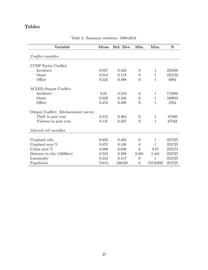
Tables

Table 2: Summary statistics: 1989-2013

Variable Mean Std. Dev. Min. Max. N

Conflict variables

UCDP Factor ConflictIncidence 0.027 0.162 0 1 225038Onset 0.014 0.119 0 1 222159Offset 0.535 0.499 0 1 6083

ACLED Output Conflict:Incidence 0.05 0.219 0 1 173893Onset 0.028 0.166 0 1 169953Offset 0.452 0.498 0 1 8762

Output Conflict: Afrobarometer surveyTheft in past year 0.313 0.464 0 1 67500Violence in past year 0.131 0.337 0 1 67533

Selected cell variables

Cropland cells 0.633 0.482 0 1 255725Cropland area % 0.072 0.138 0 1 255725Urban area % 0.009 0.039 0 0.87 255575Distance to city (1000km) 0.519 0.299 0.001 1.441 255725Luminosity 0.224 0.417 0 1 255725Population 74415 236429 0 10740200 255725

37

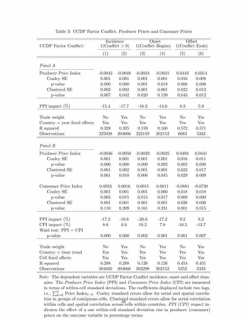
Table 3: UCDP Factor Conflict, Producer Prices and Consumer Prices

UCDP Factor Conflict:Incidence

1(Conflict > 0) 1(Onset

Conflict Begins)Offset

1(Conflict Ends)

(1) (2) (3) (4) (5) (6)

Panel A

Producer Price Index -0.0042 -0.0048 -0.0024 -0.0021 0.0443 0.0314Conley SE 0.001 0.001 0.001 0.001 0.016 0.008

p-value 0.000 0.000 0.001 0.018 0.006 0.000Clustered SE 0.002 0.002 0.001 0.001 0.022 0.012

p-value 0.007 0.042 0.020 0.139 0.043 0.012

PPI impact (%) -15.4 -17.7 -16.3 -14.6 8.3 5.9

Trade weight No Yes No Yes No YesCountry × year fixed effects Yes Yes Yes Yes Yes YesR squared 0.328 0.325 0.159 0.160 0.572 0.571Observations 225038 204666 222159 202152 6083 5333

Panel B

Producer Price Index -0.0046 -0.0050 -0.0029 -0.0025 0.0494 0.0441Conley SE 0.001 0.001 0.001 0.001 0.016 0.011

p-value 0.000 0.000 0.000 0.002 0.002 0.000Clustered SE 0.001 0.002 0.001 0.001 0.023 0.017

p-value 0.001 0.010 0.006 0.045 0.029 0.009

Consumer Price Index 0.0023 0.0016 0.0015 0.0011 -0.0881 -0.0730Conley SE 0.001 0.001 0.001 0.000 0.018 0.018

p-value 0.005 0.015 0.015 0.017 0.000 0.000Clustered SE 0.001 0.001 0.001 0.001 0.026 0.030

p-value 0.116 0.209 0.161 0.231 0.001 0.015

PPI impact (%) -17.2 -18.6 -20.0 -17.2 9.2 8.2CPI impact (%) 8.6 6.0 10.2 7.8 -16.5 -13.7Wald test: PPI = CPI

p-value 0.000 0.000 0.002 0.001 0.001 0.007

Trade weight No Yes No Yes No YesCountry × time trend Yes Yes Yes Yes Yes YesCell fixed effects Yes Yes Yes Yes Yes YesR squared 0.288 0.288 0.126 0.126 0.454 0.451Observations 204820 204666 202298 202152 5352 5333

Note: The dependent variables are UCDP Factor Conflict incidence, onset and offset dum-mies. The Producer Price Index (PPI) and Consumer Price Index (CPI) are measuredin terms of within-cell standard deviations. The coefficients displayed include two lags,i.e.,

∑2k=0 Price Indext−k. Conley standard errors allow for serial and spatial correla-

tion in groups of contiguous cells. Clustered standard errors allow for serial correlationwithin cells and spatial correlation across cells within countries. PPI (CPI) impact in-dicates the effect of a one within-cell standard deviation rise in producer (consumer)prices on the outcome variable in percentage terms.

38

Table 4: UCDP Factor Conflict, Prices and Luminosity

UCDP Factor Conflict: Incidence: 1(Conflict > 0)

(1) (2) (3)

Producer Price Index -0.0117 -0.0112 -0.0130SE 0.006 0.007 0.008p-value 0.054 0.094 0.102

Producer Price Index × luminosity 0.0089 0.0087 0.0073SE 0.005 0.005 0.005p-value 0.102 0.110 0.153

Consumer Price Index 0.0030SE 0.001p-value 0.005

Consumer Price Index × luminosity -0.0038 -0.0054 -0.0052SE 0.003 0.003 0.003p-value 0.157 0.083 0.079

PPI impact (%) at luminosity = 0 -43.5 -41.4 -48.0PPI impact (%) at luminosity = 1 -10.6 -9.2 -20.8

CPI impact (%) at luminosity = 0 11.0CPI impact (%) at luminosity = 1 -3.1 -19.9 -19.2

Country × time trend Yes N/A N/ACountry × year fixed effects No Yes YesCell FE Yes Yes YesExtra controls No No YesR squared 0.288 0.325 0.325Observations 204666 204666 204666

Note: The dependent variables is UCDP Factor Conflict incidence.The Producer Price Index (PPI) and Consumer Price Index(CPI) are measured in terms of within-cell standard deviations.The coefficients displayed include two lags, i.e.,

∑2k=0 Price

Indext−k. Standard errors allow for serial correlation within cellsand spatial correlation within countries. PPI (CPI) impact in-dicates the effect of a one within-cell standard deviation rise inproducer (consumer) prices on the outcome variable in percent-age terms. Luminosity = 1 if any light is visible at night fromsatellite images in a given cell. All specifications include controlsfor interaction effects between prices and population. Extra con-trols indicate controls for interactions between prices and threeadditional covariates: cell-level terrain, cell-level distance to thecapital city, and pre-colonial political centralization, measuredas the degree of jurisdictional hierarchy beyond the local level inthe pre-colonial ethnic polity associated with a given cell.39

Table 5: ACLED Output Conflict Incidence, Combined ProducerPrices and Consumer Prices

ACLED Output Conflict: Incidence: 1(Conflict > 0)

(1) (2) (3) (4)

Producer Price Index 0.0076 0.0073 0.0095 0.0079Conley SE 0.001 0.001 0.001 0.001

p-value 0.000 0.000 0.000 0.000Clustered SE 0.003 0.003 0.003 0.002

p-value 0.007 0.008 0.000 0.001

Consumer Price Index 0.0072 0.0040Conley SE 0.001 0.001

p-value 0.000 0.000Clustered SE 0.002 0.001

p-value 0.000 0.001

PPI impact (%) 15.1 14.4 18.9 15.8CPI impact (%) 14.4 8.0

Trade weight No Yes No YesCountry × time trend N/a N/a Yes YesCountry × year FE Yes Yes No NoCell FE Yes Yes Yes YesR squared 0.399 0.397 0.373 0.371Observations 173876 158151 158270 158151

Note: The dependent variable is a dummy for ACLED OutputConflict incidence. The Producer Price Index (PPI) and Con-sumer Price Index (CPI) are measured in terms of within-cellstandard deviations. The coefficients displayed include twolags, i.e.,

∑2k=0 Price Indext−k. Conley standard errors allow

for serial and spatial correlation in groups of contiguous cells.Clustered standard errors allow for serial correlation withincells and spatial correlation across cells within countries. PPI(CPI) impact indicates the effect of a one standard deviationrise in producer (consumer) prices on the outcome variable inpercentage terms.

40

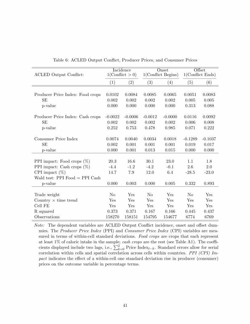
Table 6: ACLED Output Conflict, Producer Prices, and Consumer Prices

ACLED Output Conflict:Incidence

1(Conflict > 0) 1(Onset

Conflict Begins)Offset

1(Conflict Ends)

(1) (2) (3) (4) (5) (6)

Producer Price Index: Food crops 0.0102 0.0084 0.0085 0.0065 0.0051 0.0083SE 0.002 0.002 0.002 0.002 0.005 0.005p-value 0.000 0.000 0.000 0.000 0.313 0.088

Producer Price Index: Cash crops -0.0022 -0.0006 -0.0012 -0.0000 0.0116 0.0092SE 0.002 0.002 0.002 0.002 0.006 0.008p-value 0.252 0.753 0.478 0.985 0.071 0.222

Consumer Price Index 0.0074 0.0040 0.0034 0.0018 -0.1289 -0.1037SE 0.002 0.001 0.001 0.001 0.019 0.017p-value 0.000 0.001 0.013 0.015 0.000 0.000

PPI impact: Food crops (%) 20.3 16.6 30.1 23.0 1.1 1.8PPI impact: Cash crops (%) -4.4 -1.2 -4.2 -0.1 2.6 2.0CPI impact (%) 14.7 7.9 12.0 6.4 -28.5 -23.0Wald test: PPI Food = PPI Cash

p-value 0.000 0.003 0.000 0.005 0.332 0.893

Trade weight No Yes No Yes No YesCountry × time trend Yes Yes Yes Yes Yes YesCell FE Yes Yes Yes Yes Yes YesR squared 0.373 0.371 0.167 0.166 0.445 0.437Observations 158270 158151 154795 154677 6774 6769

Note: The dependent variables are ACLED Output Conflict incidence, onset and offset dum-mies. The Producer Price Index (PPI) and Consumer Price Index (CPI) variables are mea-sured in terms of within-cell standard deviations. Food crops are crops that each representat least 1% of caloric intake in the sample; cash crops are the rest (see Table A1). The coeffi-cients displayed include two lags, i.e.,

∑2k=0 Price Indext−k. Standard errors allow for serial

correlation within cells and spatial correlation across cells within countries. PPI (CPI) Im-pact indicates the effect of a within-cell one standard deviation rise in producer (consumer)prices on the outcome variable in percentage terms.

41

Table 7: Afrobarometer Output Conflict: Triple Difference

Theft Violence

(1) (2) (3) (4)

Producer Price Index: Food crops -0.0101 0.0284 -0.0000 0.0089SE 0.007 0.005 0.005 0.009p-value 0.158 0.000 0.997 0.331

Producer Price Index: Food crops × farmer 0.0082 0.0097 0.0098 0.0067SE 0.008 0.008 0.006 0.005p-value 0.336 0.216 0.080 0.150

Producer Price Index: Food crops × trader 0.0242 0.0258 0.0007 0.0009SE 0.012 0.014 0.009 0.006p-value 0.043 0.064 0.938 0.894

Producer Price Index: Cash crops -0.0037 -0.0131 0.0044 -0.0139SE 0.012 0.013 0.008 0.009p-value 0.753 0.332 0.564 0.138

Producer Price Index: Cash crops × farmer -0.0365 -0.0409 -0.0152 -0.0145SE 0.012 0.012 0.006 0.004p-value 0.003 0.001 0.016 0.001

Producer Price Index: Cash crops × trader -0.0230 -0.0167 -0.0077 -0.0051SE 0.015 0.010 0.016 0.012p-value 0.115 0.087 0.636 0.685

Consumer Price Index 0.0401 -0.0363SE 0.030 0.027p-value 0.186 0.173

PPI Food − PPI Cash treatment effect: farmers 0.0446 0.0506 0.0250 0.0212SE 0.016 0.017 0.009 0.008p-value 0.006 0.005 0.007 0.010

PPI Food − PPI Cash treatment effect: traders 0.0472 0.0425 0.0084 0.0059SE 0.020 0.018 0.019 0.015p-value 0.017 0.021 0.665 0.696

PPI impact: Food (%) -3.2 9.1 -0.0 6.8× farmer 2.6 3.1 7.5 5.1× trader 7.7 8.2 0.5 0.7

PPI impact: Cash (%) -1.2 -4.2 3.4 -10.6× farmer -11.7 -13.1 -11.6 -11.1× trader -7.4 -5.3 -5.9 -3.9

CPI impact (%) 12.8 -27.8Country × time trend Yes N/a Yes N/aCountry × period fixed effects No Yes No YesControls Yes Yes Yes YesArea fixed effects Country Cell Country CellSurvey round fixed effects Yes Yes Yes YesR squared 0.036 0.069 0.033 0.058Observations 39873 39036 39925 39090

Note: The dependent variables are binary responses to survey questions that ask whetherindividuals over the previous year (i) have been victims of theft; (ii) have been victims ofphysical assault. The Producer Price Index (PPI) and Consumer Price Index (CPI) vari-ables are measured in terms of within-cell standard deviations. Food crops are crops thateach represent at least 1% of caloric intake in the sample; cash crops are the rest (see Table

A1). The coefficients displayed include four lags, i.e.,∑4

k=0 Price Indext−k, where eacht is a six-month period. Farmer indicates that the respondent is a commercial farmer;trader indicates that the respondent is a trader, hawker or vendor. Standard errors allowfor serial correlation and spatial correlation within cells. PPI (CPI) Impact (%) indicatesthe effect of one within-cell standard deviation rise in producer (consumer) prices on theoutcome variable in percentage terms.

42

Table 8: Summary of Naive Regression Results

UCDP Conflict ACLED Conflict

Panel A: Producer Price Index

Producer Price Index -0.0054 0.0102SE (0.021) (0.007)p-value 0.795 0.165impact (%) -1.1 1.1

Panel B: Consumer Price Index

Consumer Price Index 0.0251 0.0197SE (0.023) (0.013)p-value 0.282 0.134impact (%) 5.1 2.2

Panel C: Both Indices

Producer Price Index -0.0326 -0.0048SE (0.023) (0.012)p-value 0.155 0.690impact (%) -6.7 -0.5

Consumer Price Index 0.0435 0.0223SE (0.029) (0.019)p-value 0.135 0.244impact (%) 8.9 2.5

Note: This table summarizes results from six separate country-level re-gressions that each include controls for country fixed effects and country-specific time trends. The outcome variables respectively measure the inci-dence of UCDP conflict events and the combined ACLED conflict events.In Panel A, only the PPI is included; in Panel B, only the CPI is in-cluded; in Panel C, both the PPI and the CPI are included. The coef-ficients displayed include two lags, i.e.,

∑2k=0 Price Indext−k. Standard

errors are clustered at the country level. Impact (%) indicates the effectof a within-cell one standard deviation rise in producer (consumer) priceson the outcome variable in percentage terms.

43

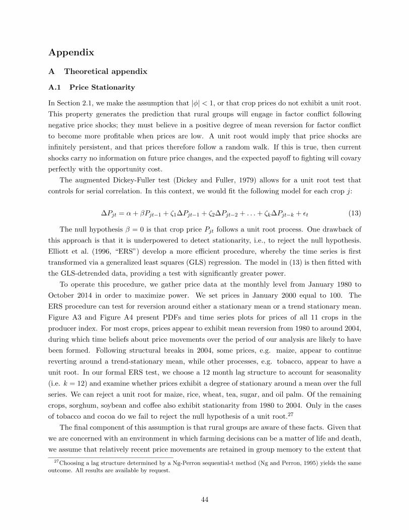
Appendix

A Theoretical appendix

A.1 Price Stationarity

In Section 2.1, we make the assumption that |φ| < 1, or that crop prices do not exhibit a unit root.

This property generates the prediction that rural groups will engage in factor conflict following

negative price shocks; they must believe in a positive degree of mean reversion for factor conflict

to become more profitable when prices are low. A unit root would imply that price shocks are

infinitely persistent, and that prices therefore follow a random walk. If this is true, then current

shocks carry no information on future price changes, and the expected payoff to fighting will covary

perfectly with the opportunity cost.

The augmented Dickey-Fuller test (Dickey and Fuller, 1979) allows for a unit root test that

controls for serial correlation. In this context, we would fit the following model for each crop j:

∆Pjt = α+ βPjt−1 + ζ1∆Pjt−1 + ζ2∆Pjt−2 + . . .+ ζk∆Pjt−k + εt (13)

The null hypothesis β = 0 is that crop price Pjt follows a unit root process. One drawback of

this approach is that it is underpowered to detect stationarity, i.e., to reject the null hypothesis.

Elliott et al. (1996, “ERS”) develop a more efficient procedure, whereby the time series is first

transformed via a generalized least squares (GLS) regression. The model in (13) is then fitted with

the GLS-detrended data, providing a test with significantly greater power.

To operate this procedure, we gather price data at the monthly level from January 1980 to

October 2014 in order to maximize power. We set prices in January 2000 equal to 100. The

ERS procedure can test for reversion around either a stationary mean or a trend stationary mean.

Figure A3 and Figure A4 present PDFs and time series plots for prices of all 11 crops in the

producer index. For most crops, prices appear to exhibit mean reversion from 1980 to around 2004,

during which time beliefs about price movements over the period of our analysis are likely to have

been formed. Following structural breaks in 2004, some prices, e.g. maize, appear to continue

reverting around a trend-stationary mean, while other processes, e.g. tobacco, appear to have a

unit root. In our formal ERS test, we choose a 12 month lag structure to account for seasonality

(i.e. k = 12) and examine whether prices exhibit a degree of stationary around a mean over the full

series. We can reject a unit root for maize, rice, wheat, tea, sugar, and oil palm. Of the remaining

crops, sorghum, soybean and coffee also exhibit stationarity from 1980 to 2004. Only in the cases

of tobacco and cocoa do we fail to reject the null hypothesis of a unit root.27

The final component of this assumption is that rural groups are aware of these facts. Given that

we are concerned with an environment in which farming decisions can be a matter of life and death,

we assume that relatively recent price movements are retained in group memory to the extent that

27Choosing a lag structure determined by a Ng-Perron sequential-t method (Ng and Perron, 1995) yields the sameoutcome. All results are available by request.

44

stationarity can be detected while present.

A.2 Bargaining

Chassang and Padro i Miquel (2009) characterize the role of bargaining in a perfect information

environment with offensive advantages. We begin with same set up as that described in Section 2.1,

except for two differences. First, groups now begin with unequal landholdings, so that group 1

controls N2 + λ, and group 2 controls N

2 − λ. Second, we make the assumption, without loss of

generality, that the game has a duration of only one period.

Groups can engage in bargaining in order to avert conflict. A transfer will avert conflict if and

only if neither side has an incentive to deviate following the transfer. Only then can groups credibly

commit to peace (Fearon, 1995). Let T represent the transfer that group 1 can give group 2 to

deter an attack. The condition for group 1 to prefer this to conflict is therefore

P · (N

2+ λ−T) > π(1− v)[P ·N].

The left hand side is the value of group 1’s post-transfer landholding. The right hand side

represents the expected payoff from launching a unilateral attack, where again π is the probability

of victory for the attacker, and v is the opportunity cost of conflict.

For peace to prevail, the transfer must also generate a situation in which group 2 also prefers

post-transfer peace to the expected payoff from a unilateral attack. This condition is given by

P · (N

2− λ+ T) > π(1− v)[P ·N].

It follows that the transfer must satisfy

P · N2> π(1− v)[P ·N]. (14)

The is the condition for peace in the presence of bargaining. Two observations are noteworthy.

First, λ does not appear in the condition. The initial distribution of land does not determine

conflict. Second, the set of parameters for which there exists a transfer T that avoids conflict is

the same set of parameters for which an equal distribution of land N2 guarantees peace. Peace is

therefore only attainable if there exists no profitable unilateral deviation when both groups have

equal landholdings. This holds for any initial land distribution.

The intuitive interpretation is that bargaining allows groups who are satisfied with their peaceful

status quo to avoid war by transferring land to a dissatisfied group. Hence, bargaining can avoid

war only in situations where one group is satisfied and the other is not. In this case of perfect

information, bargaining can therefore only assuage the threat of conflict that is driven by unequal

landholdings. When condition (14) does not hold, bargaining cannot affect the prospect of violence

caused by the first-mover advantage.

45

Rearrange condition (14), conflict occurs if

π > πw ≡ 1

2(1− v). (15)

Peace is destabilized only if the first-mover advantage is substantial. Indeed, as noted in Chas-

sang and Padro i Miquel (2009), there exists an offensive advantage for π ∈ (12 , πs) in which no

conflict will occur because fighting entails an opportunity cost v. The larger it is, the larger the

first-mover advantage needs to be in order to generate violence.

A.3 Threshold P

In this section, we characterize the threshold P below which realizations of P lead to conflict by

applying Chassang and Padro i Miquel (2009) to our setting. Consider the continuation value of

peace as the highest solution to the following equation:

V P = F (P)1

2

[E(P ·N | P < P)(1− v) + δV A

]+

(1− F (P)

)[E(P · N

2| P > P) + δV P

].

With probability F (P), the realization of P falls below P, and war ensues. Solving for V P

yields

V P =Y

2(1− δ)−vF (P)E(P · N2 | P < P)

1− δ(

1− F (P)) (16)

The future value of playing peace in this equilibrium equals the value of playing peace forever

minus the expected cost of war that will occur as soon as Pt < P. This is decreasing in P because

the larger is the threshold P, the higher the probability that conflict will occur. This increases the

losses for two reasons: first, conflict occurs sooner in expectation, hence costs are less discounted;

second, a higher threshold P implies that the expected value of the resources lost in the war is

larger.

The optimal threshold P is the lowest value of Pt that satisfies (1) with equality. We substitute

in (2) and (16) and rearrange to find

P =δ

1− 2π(1− v)

[(2π − 1)

P

1− δ+vF (P)E(P | P < P)

1− δ(

1− F (P)) ]

. (17)

Existence of P is guaranteed because the right hand side is always strictly positive, bounded

and continuous.28 In contrast, the left hand side can take any value in (0,+∞). It follows that

there are values of P that can be higher or lower than the right hand side. We can then say that, for

π < πW , the most efficient subgame perfect equilibrium is given by the smallest positive solution

to (17). As above, for any first-mover advantage that yields π > πW , there is no equilibrium that

28The right hand side can written as δ[πV A−V P ]1−2π(1−v)

, which has an upper bound δπ1−2π(1−v)

P·N1−δ .

46

avoids war at t = 1, for any P1.

Note that the equilibrium threshold is increasing in π and δ, and decreasing in v. This implies

that conflict is more likely to occur in the presence of higher offensive advantages and, interestingly,

higher levels of patience. The latter can be explained by the fact that the costs of conflict are

immediate, while the potential spoils are realized into the future. Finally, and intuitively, the

likelihood of war is decreasing in the opportunity cost of fighting.

A.4 Deriving consumer effects of food crops, cash crops, and imported food crops

In this section, we derive how changes in the prices of food crops, cash crops, and import crops

affect conflict. These results are summarized in Section 2.2 of the main text.

Food crops We begin with Pf , the price of food crops that are both produced and consumed in

a given cell. Again denoting by A the left hand side of (5), and by W the right hand side, we first

make the simple observation that

dAdPf

=Q(LQ)Nf (L− LQ)

LQ> 0. (18)

Higher food crop prices increase the payoff from appropriation.

In determining the effect of Pf on W, we exploit a fundamental property of food: it is essential

to survival, and cannot be substituted. We therefore assume without loss of generality that the

price elasticity of demand is zero, and characterize the real wage rate as wPf

. If nominal wages are

rigid in the short run, we obtain:

dWdPf

= −[1−Q(LQ)

]w

P 2f

< 0. (19)

Proposition 2. In food-producing cells, higher food prices Pf will increase the incidence of output

conflict in the short run.

The proof comes from (18) and (19). Equation (18) must be positive, as LQ < L is a necessary

condition for appropriation to exist. Without it, there would be no output to appropriate. By

contrast, equation (19) must be negative, yielding a clear prediction. We obtain the same qualitative

outcome if nominal wages adjust fully to higher prices such that real wages are unchanged, asdAdPf− dW

dPf= dA

dPf> 0.29

29While it is not a critical assumption, Ivanic et al. (2012) do suggest that the 2011 food price spike reduced netconsumers’ real wages in rural regions. However, in the longer run nominal wages will rise with higher prices by anamount determined by factor markets. Taking this into account, we can quantify the total effect of the price changeon real wages as:

Pf (1−Q(LQ)) dwdPf− (1−Q(LQ))w

P 2f

(20)

where dwdPf

=1−aN dr

dPf

aL, which is obtained from taking the total differential of equation (4). If price increases are paid

47

The intuition of Proposition 2 is straightforward: higher food prices increase the value of output

that accrues to landowners (generating a predation effect), while simultaneously decreasing the real

wage of laborers in the short run (generating an income effect). This combination of effects increases

the profitability of output conflict relative to productive wage labor.30

Cash crops We now consider the effect of a change in Pc, the price of crops that are produced

in a given cell but consumed elsewhere. The key feature of Pc is that it will not feature as a wage

deflator, in contrast to the case above. It can thus be considered as a non-food crop like tobacco or

cotton, or edible crops that do not contribute significantly to caloric intake, such as tea or coffee.

As in the case above, higher prices will increase the value of appropriable surplus by an amount:

dAdPc

=Q(LQ)Nc(L− LQ)

LQ> 0. (21)

However, higher prices will also increase real wages by an amount:

dWdPc

=[1−Q(LQ)

][1− aN drdPc

aL

], (22)

which is larger than zero provided aNdrdPc

< 1; in other words, as long as landowners do not accrue

fully the gains from higher prices.31 We thus have a predation effect in (21) caused by the rise in

value of appropriable output, but also a positive income effect in (22) caused by an increase in real

wages in the productive sector. This generates an ambiguous effect overall: higher cash crop prices

Pc may increase or decrease output conflict. We can say with confidence that the effect of Pc on

output conflict will be lower than the effect of Pf .

Proposition 3. The effect of cash-crop prices Pc on equilibrium output conflict is lower than the

effect of food-crop prices Pf on equilibrium output conflict.

This is because Pc and Pf both increase the value of appropriable surplus, generating a predation

effect, but only Pf will reduce real wages; Pc will increase real wages provided aNdrdPc

< 1.

Import crops We finally consider the effect of a change in Pm, the price of imported food crops.

By definition, import crop prices will only affect conflict in net consumer cells. As crop m is not

produced domestically, the nominal values of both the spoils of appropriation and of the productive

sector wage are unaffected by a price change. However, as both are deflated by Pm, and as A = Win equilibrium, it follows that:

fully to land, i.e. if aNdrdPf

= 1, then (20) is the same as (19). As aNdrdPf

falls, (20) approaches zero.30If we relax the assumption of a single productive sector to include also non-agricultural productive activities, we

would expect the average magnitude of the effect to be even larger. This is because, for workers in the non-farmsector, nominal wages will be slower to increase with food prices, resulting in a larger decline in real terms.

31Dube and Vargas (2013) find that higher coffee prices reduce conflict in Colombia for this reason. In Dal Bo andDal Bo (2011), this is because coffee prices are relatively labor intensive.

48

dAdPm

= − AdP 2

m

=dWdPm

= − WdP 2

m

. (23)

Income is spent on food, and so as prices rise, the real value of appropriation declines in concert

with real wages. We therefore have no substitution effect between appropriation and wage labor:

a change in Pm generates a pure income effect only.

Under what conditions will this cause consumers to engage in conflict? To answer this, we

must first consider optimal responses to food price shocks. In Appendix Section A.5, we make the

following points: (i) agents are unwilling to substitute food consumption intertemporally; (ii) in

order to maintain food consumption in the wake of price shocks, therefore, agents must have access

to savings, credit, or insurance; (iii) absent these mechanisms, agents must resort to costly coping

strategies (Chetty and Looney, 2006).

We proceed in the spirit of this final point, as financial markets are relatively undeveloped in

Africa. To illustrate, consider a net consumer earning a fixed nominal wage wl from productive

activities. Indirect utility V (Pm, wl) depends on the price of food items (produced elsewhere) and

wage income. Consumption is determined by the budget constraint wl ≥ PmC, and C ≥ bCc; that

is, consumption must be weakly greater than a target caloric intake.32 If this restriction is violated,

utility is 0.33 We therefore assume without loss of generality that u seeks to maximize utility

at time t, and we abstract from future concerns. Denote by P lm the price of food that prevents

utility-maximizing consumers with income wl from achieving consumption C ≥ bCc. That is,

V (P lm, wl) = 0.

We first consider the effect of Pm on factor conflict by introducing to the environment the

existence of armed group activity.34 Armed groups offer to potential fighters a wage ww. For

(wage) fighters, expected utility is therefore given by:

E[V w(Pm, w

w, φu)]

= V (Pm, ww)− φu,

where φu ∈ (0, φ∗u] can be considered as the expected cost for consumer u of incurring physical of

psychic harm in battle, and E[V w(Pm, w

w, φ∗u)]

= 0 for any Pm. Importantly, φu has no direct

effect on u’s current budget constraint. Denote by lu ∈ {0, 1} the decision to allocate labor either

to productive activities or armed fighting, where l = 1 implies that he chooses to work in the

productive sector. The net consumer therefore faces the following problem:

maxlu∈{0,1}

Vu = lu(V (Pm, wl)) + (1− lu)(V (Pm, w

w)− φu). (24)

32This condition may reflect the desire to avoid a poverty trap of the type discussed in Dasgupta (1997).33This set up could be described with a standard Stone-Geary functional form, where C ≥ γ is the subsistence

consumption requirement, and wl ≥ pγ the budget constraint.34This can be caused by a realization Pct < P for export cash crops such as cocoa beans, rubber, cotton or tobacco,

or through another exogenous mechanism.

49

Rearranging the solution, he will fight if

V (Pm, ww)− V (Pm, w

l) > φu. (25)

In other words, net consumers will fight if the war wage premium offsets the expected cost of

fighting. This admittedly simple condition gives rise to the following observation: if wl ≥ ww, then

net consumers will not fight, for any Pm, φu. We obtain this result from our characterization of φu,

which is strictly positive.

The more interesting case arises when wl < ww, i.e., when agents earn a wage lower than that

offered by armed groups. We are specifically interested in the effect of food prices on the decision to

fight in this context. It is here that our assumption of nonlinearity in consumption comes to effect.

Without it, rising prices would have an ambiguous effect on u’s choice: a higher P ′m would impose

a proportionate drop in real wages from both war (ww

P ′m) and productive activities ( w

l

P ′m), rendering

the decision unchanged (as in (23)). But if we explicitly take the target consumption constraint

into account, a clearer picture emerges.

Consider a price increase to P lm. We can say with certainty that P lm < Pwm, as wl < ww. This

yields a “fighting condition” for net consumers as follows:

V (P lm, ww)− V (P lm, w

l) > φu. (26)

The first term must be positive, as P lm < Pwm. Wages are sufficiently high to guarantee subsistence,

which yields a strictly positive utility. The second term is 0 by definition: wl cannot return positive

utility when prices reach P lm. The decision to fight, therefore, is determined by the condition

V (P lm, ww) > φu, which is true when φu < φ∗u. In other words, net consumers will fight as long

as the expected value of doing so yields any utility larger than 0. Only those who expect with

probability 1 to incur costs φ∗u will be indifferent between fighting and not fighting.35 Other net

consumers for whom wl < ww will join the armed group, provided they do not have access to

superior outside options, including conventional consumption-smoothing instruments.

Observation 1. In the absence of financial consumption-smoothing instruments, a realization of

imported food crop price Ptm ≥ P lm will increase the probability that net consumers earning w ≤ wl

will join factor conflict groups.

The intuition is straighforward. Higher food prices force those close to subsistence to increase

their labor supply in order to maintain a target consumption level. In the absence of alternative

options, this can imply incurring significant costs. It is worth reflecting on three striking empirical

examples. First, de Janvry et al. (2006) find that Mexican households withdraw children from

education as a response to adverse income shocks. Second, Dupas and Robinson (2012) find that

transactional sex workers in Kenya engage in riskier—and more lucrative—sexual behavior following

35This is because u(0) ≤ E[u(0)]: a positive probability of any utility larger than 0 dominates a guaranteed utilityof 0.

50

an income shock caused by widespread political violence in 2007. Finally, Miguel (2005) finds that

weather shocks in Tanzania lead to a large spike in “witch” killings—the murder of elderly women,

typically by relatives.36 All three of these risk-coping mechanisms share the same properties of φ:

they are each costly, whether in terms of future income, expected health or social health, but they

also each permit an expansion of the current budget constraint that allows marginal households to

achieve a target consumption level. In our setting, we make the connection between these costly

coping mechanisms and the decision to join armed conflict groups in battle.

The same logic can be applied to the decision to engage in output conflict. Higher food prices

induce those at the margin of a target consumption level to engage in costly or risky activities in

order to maintain consumption. In this case, food is not produced domestically, and consumers turn

to property crime (which may also take the form of riots and looting) as a means of appropriating

goods.37 This gives an analogous prediction as follows:

Observation 2. In the absence of financial consumption-smoothing instruments, a realization of

staple food crop prices Ptm ≥ P lm will increase the probability that net consumers earning w ≤ wl

will engage in output conflict.

A.5 Consumption and intertemporal substitution

A large literature examines the optimal response to income variation over the life cycle through the

lens of consumption smoothing, or the process of saving and dissaving in order to maintain a high

marginal utility of consumption.38 However, it does not necessarily follow that perfect consumption

smoothing is always optimal in context of price variation. If consumers expect prices to be lower

in future, it may be optimal to reduce consumption in the present period. For example, consider a

utility function with constant relative risk aversion:

U(Cjt) =

C1jt−σ1−σ for σ > 0, σ 6= 1

ln Cjt for σ = 1, (27)

where Cjt is consumption of staple food j in time t, Pjt is the price of j, and σ is the risk aversion

parameter. Under the assumption of perfect capital markets, intertemporal substitution can be

determined by

CjtCjt+1

=

(Pjt+1

Pjt

) 1σ

.

Thus, consumption at t relative to future consumption is inversely related to the price at t relative

to the future price. The extent to which consumers will adjust current consumption is determined

36Oster (2004) identifies analogous behavior in the context of temperature shocks in medieval Europe, reinforcingthe case that there is little inherently “African” about costly coping strategies in the face of extreme poverty.

37This is akin to Gould et al. (2002), who find that lower wages for unskilled men in the US drove crime rates inthe 1980s and 1990s.

38This follows seminal contributions on the permanent income and life cycle hypotheses by Friedman (1957) andModigliani and Ando (1957) respectively. A recent review is provided in Jappelli and Pistaferri (2010).

51

by σ, the measure of risk aversion. A lower σ implies a higher substitution effect. Our assumption

reflects evidence in Alem and Soderbom (2012): in the context of staple food consumption in Africa,

σ is high, and consumers are less willing to substitute across periods.

This implies that consumers require liquidity to maintain a target caloric intake for a given

price increase. For those with access to savings, insurance or credit, this may be achieved. For

those without recourse to these instruments, relative consumption must decrease in proportion to

the price change so that expenditure does not exceed nominal income earned in period t, unless

other avenues are pursued.

Given that our focus is on Africa, formal financial services are not assumed to be available

to a significant portion of our sample. We must then ask, how prevalent are informal smooth-

ing instruments in developing countries? Early work by Paxson (1992) and Townsend (1994) in

India, and by Udry (1994, 1995) in Nigeria, suggests a significant role for time series (savings)

and cross-sectional (insurance) smoothing mechanisms, to the extent that Morduch (1995) ques-

tions the relative efficiency of publicly provided formal alternatives. However, subsequent research

challenges this interpretation on two complementary counts. First, consumption appears to be

strongly affected by income shocks, particularly within poor subgroups (Ravallion and Chaudhuri,

1997; Morduch, 1999; Dercon, 2004). Second, observed consumption changes may not capture the

severity of household welfare costs induced by income shocks. This reflects the argument in Chetty

and Looney (2006): for households that are close to subsistence (that is, a high σ case) and that do

not have access to financial smoothing instruments, a target consumption level must be maintained

through costly coping strategies.

B Data appendix

B.1 Price data

Table A1 presents the descriptions and sources for each raw price variable used to construct the

price indices in the analysis. For each crop price, we present the exact description provided by

the source. In the third column, we indicate whether the data came from the IMF International

Finance Statistics or the World Bank Global Economic Monitor. In the following column we

indicate whether or not the crop constituted part of the consumer index. In the final column, we

indicate whether or not the crop constituted part of the producer index, and if so, whether we

coded it as a food crop (which each occupy over 1% of calories consumed in a country over the

series), or a cash crop (the rest). For crops with more than one potential price measure (i.e., coffee

and tobacco), we compute indices using the the average value.

B.2 Alternate factor conflict measure

In robustness tests, we also operate an alternative measure of factor conflict. It consists of a subset

of the Armed Conflict Location and Event Data (ACLED) project, running from 1997 to 2013 (see

Raleigh et al., 2010). Like the UCDP project, ACLED records geocoded conflict events from a range

52

of media and agency sources. Of eight conflict event categories included in the data, we include

only battles in which non-state actors have won territory (category 2). This has the advantage of

capturing events that are consistent our theoretical definition of factor conflict. However, with a

sample mean of only 0.04%, it is a somewhat rare event in the data, reflecting the possibility that

it represents a small subset of factor conflict events over the period. Broadening the measure to

incorporate other battle types would run the risk of including events that fall within the scope of

output conflict, as the threshold for inclusion is significantly lower than that of our preferred UCDP

measure (Eck, 2012).39

C Additional results

C.1 Robustness of factor conflict results

Additional covariates Tables A2 to Table A4 include potentially important omitted variables.

We note above that global prices are affected by weather events in producer countries. If those

weather events are associated with global weather patterns, such as the El Nino Southern Oscil-

lation (ENSO), then it could be the case that local weather events generate a correlation between

global prices and the error term (Burke et al., 2015). We therefore introduce a set of weather

variables. Temperature is the cell-year mean temperature in degrees celsius, based on monthly

meteorological statistics from the US National Oceanic and Atmosphere Administration. Drought

variables are aggregated Standardized Precipitation Index (SPI6) measures that indicate within

cell-year deviations in precipitation based on monthly data. Moderate drought indicates that there

were at least three consecutive months in which rainfall was more than 1 standard deviation below

long term (six-month) levels; severe drought indicates that there were at least two months during

which rainfall was more than 1.5 standard deviations below long term levels; and extreme drought

indicates that both of these criteria were met in a cell-year. These data are provided by the Global

Precipitation Climatology Centre, and converted to grid format by the PRIO-GRID project (Tollef-

sen et al., 2012). Table A3 presents results from specifications that include these covariates where

standard errors are two-way clustered to allow for serial correlation at the cell-level and spatial

correlation at the country level. Table A4 presents results with Conley standard errors that allow

for serial and spatial correlation in groups of contiguous cells, which is likely to be more appropriate

given the localized nature of weather patterns. We see evidence that high temperatures and severe

drought do increase the probability of factor conflict incidence. Neither price index estimate is

significantly affected by their inclusion.

Ross (2015) documents a large body of evidence suggesting a link between oil production and

conflict. Although global oil prices are not believed to be causally related to global food prices

(see Dillon and Barrett, 2015), a spurious correlation could nonetheless bias our price estimates.

We therefore test three mechanisms through which oil prices can affect cell-level factor conflict

in Table A4. First, higher prices in oil producing cells could increase violence by either funding

39This would lead to non-classical measurement error that would bias our producer price estimate toward zero.

53

insurgency (Collier and Hoeffler, 2004) or provoking predation (Dube and Vargas, 2013). Second,

higher prices in oil producing countries could also strengthen a state’s capacity to repel violence,

generating a negative impact on conflict (Fearon and Laitin, 2003). Third, higher oil prices could

increase violence through the same inflationary channel we explore in this study in the context of

food. We obtain geocoded data on the location of oil fields in Africa from the PRIO Petroleum

Dataset.40 We combine this with IMF data on world oil prices to estimate a specification with

three oil variables: an oil price × cell-level dummy for the presence of an oil field; an oil price ×country-level dummy for oil producers; and an oil price variable that varies independently. We also

add a second specification containing the cell-level interaction and country × year fixed effects. We

present both models for incidence, onset and offset. We first note that the producer index estimate

remains largely unaffected across specifications. The consumer price index effect is significant in the

onset specification, but not in the equivalent offset model. The cell-level oil price measure has no

significant effect on factor conflict; the country-level price measure has a negative effect, consistent

with the state capacity interpretation of analogous results in Bazzi and Blattman (2014); and the

oil price variable increases conflict incidence while controlling for production effects—a result we

interpret as consistent with our consumer price effect.

Additional robustness Several alternative specifications are estimated for robustness. In Ta-

ble A5, we compare models with UCDP Factor Conflict and ACLED Territorial Change as out-

comes. In the first column we analyze ACLED Territorial Change over the maximum sample period

from 1997 to 2013. Both price indices enter with the expected signs, but neither coefficient is sig-

nificant at conventional levels. In columns (2) and (3) we set both side-by-side over the intersection

of sample years (1997-2010). We note that PPI and CPI impacts in terms of the outcome mean are

very similar: -28% and 1.1% for the ACLED measure and -25.3% and -1% for the UCDP measure.

In both models PPI effects are significant; the p-values for the CPI effects are similar; and difference

between the PPI and CPI effects are also significant. This exercise indicates that the main results

of this study are likely not driven by fixed features of the two data-collection organizations.

In Table A6, we aggregate our spatial unit of analysis from 0.5 degree × 0.5 degree cells to 1

degree× 1 degree cells. The outcome variable now indicates that a conflict event took part in a given

cell of roughly 110km × 110km, and the producer price index is averaged over four of the baseline

cells. This loss of information can be expected to push the estimates toward zero. However, this

exercise can also address concerns that the high degree of spatial resolution is artificially increasing

the magnitude of the producer price coefficients. In addition to this adjustment, we explicitly model

spatial dependence in the producer price index. This is achieved by first generating a symmetric

weighting matrix W, which ascribes a value of 1 to all eight contiguous cells, and a value of 0

otherwise. A spatial lag of producer prices is then created by multiplying this matrix by the vector

of observations.41 This is a spatial Durbin model (Anselin, 2013), and is applied in a similar

40The dataset contains information on all known on-shore oil and gas deposits throughout the world. It can beaccessed at https://www.prio.org/Data/Geographical-and-Resource-Datasets/Petroleum-Dataset

41We also include the sum of temporal lags in the spatial lag variable.

54

set-up by Harari and La Ferrara (2014) in their disaggregated analysis of weather and conflict in

Africa. We also include Conley standard errors (in groups of contiguous cells) as well as two-way

clustered errors (at the level of the cell and the country-year). A unit increase in the spatial

lag variable reflects a unit increase in any of the eight contiguous cells. The results indicate the

following: although standard errors are larger, the PPI still increases factor conflict incidence and

duration in our preferred country × year models; producer prices in neighboring 1 degree cells do

not significantly influence conflict in a given cell; and the CPI effects are largely unaffected given

that they vary at the country-year level.

In Table A7, we present results from a fixed effects conditional logit estimation. The main results

are qualitatively similar, although now higher producer prices significantly reduce the duration of

factor conflict only, and the opposite is true for consumer prices, as in the main specification. These

specifications include a common trend and no country × year fixed effects in order for the models

to converge. The sample size is also significantly smaller, as the CL estimator discards cells that

exhibit no change in the outcome variable over the series.

C.2 Robustness of output conflict results

Table A8 presents results from the baseline output conflict regression that includes country × year

fixed effects and therefore excludes the CPI variable. These results reinforce the main findings, and

are discussed in Section 5 of the main text.

In Table A9 and Table A10, we reintroduce the weather and oil price variables that are described

above. Firstly, we note that the main results are mostly unchanged. Higher food crop prices lead to

large and significant increases in output conflict in food-producing areas. Higher cash crop prices

lead to negligible changes in output conflict in cash crop producing areas. The coefficients for the

consumer price index are large and significant in the weather regressions, but are smaller and not

significant when all three oil price variables are included. Interestingly, however, higher oil prices for

consumers—i.e., controlling for production at both the cell and country level—significantly increase

output conflict incidence and duration, a result we interpret as consistent with our model. We also

find that higher oil prices have an additional effect on output conflict in oil-producing cells.

In Table A11 we repeat the spatial Durbin model aggregated to 1 degree cells and including both

Conley and two-way clustered standard errors. Models with and without CYFEs are presented for

each one of the the incidence, onset and offset outcomes. Again, βpc < βpf in all incidence and

onset regressions, while the coefficients are not significantly different in the offset regressions. In

most cases, a higher PPI for food crops increases output conflict and higher PPI for cash crops

reduces output conflict. The CPI has a large effect on incidence, onset and duration. Focusing on

the CYFE regressions in columns (2), (4) and (6), we see some evidence that a rising PPI for food

crops in neighboring cells reduces conflict duration, perhaps reflecting the possibility that output

conflict shifts to neighboring cells when crop prices are higher there.

In Table A12 we present results from a FE conditional logit estimator with and without trade

weights for each of the three outcomes. On this occasion we lose around three quarters of our

55

observations, as cells that do not exhibit changes in the dependent variable over the series do not

contribute to the log-likelihood. P-values are slightly above the 10% threshold on the PPI food

crop coefficient when trade weights are not included, while estimates are extremely noisy when

weights are used. The cash crop producer price index is never associated with more violence. The

coefficients on the the two PPI measures are significantly different (in the expected direction) in

the incidence and onset regressions when trade weights are not used. The consumer price index

estimate is also consistent with the LPM results.

Is output conflict just “food riots”? Our theory above predicts that the effect of higher

consumer prices on output conflict is positive because agents will engage in such conflict as a

means of maintaining a target consumption level. However, work by Bellemare (2015) and others

show that higher food prices can cause “food riots” that may be driven as much by a desire to

provoke government policy changes than by a desire to directly appropriate property from others,

an interpretation supported by Hendrix and Haggard (2015) and Bates and Carter (2012), who

find that governments frequently alter policies in favor of consumers in the wake of price shocks.

Food riots in the context above will occur in urban centers where government authorities can be

expected plausibly to respond. Output conflict, according to our theory, can happen anywhere

there are poor consumers and where there is appropriable property. We therefore interact our

consumer price index with two measures of urbanization in order to detect these differences. The

first measures the share of each cell area that is classified as urban by the SEDAC project at

Columbia University introduced above; the second captures the population share that is classified

as urban. Evidence of a significant interaction term is consistent with this protest riot explanation

(although it does not rule out the possibility that output conflict is more pervasive in cities).

However, a significant coefficient on the CPI term strongly suggests that the overall effect is not

explained fully by protest riots.

Results are given in Table A13. In column (1), both the interaction term CPI × urban area

and the CPI term are significantly different from zero (the respective p-values are 0.00 and 0.03).

In the 90th percentile of urbanization, a standard deviation rise in the CPI in increases output

conflict by 12%; when urban area is equal to zero, the same change still increases output conflict by

4.6%. In column (2), we add CYFEs and remove the CPI term. We see that, while the interaction

term is still significant, it is also smaller. In columns (3) and (4) the interaction term CPI ×urban population is used as a substitute, and we find that its effect is statistically indistinguishable

from zero irrespective of whether CYFEs are included. Taken together, these results suggest that

the main output conflict results are not driven by urban food riots or protests designed to create

unrest and agitate for policy reforms. Output conflict occurs in non-urban as well as urban areas,

consistent with our main theoretical prediction. The additional effect in urban areas is consistent

not only with the idea that consumers demonstrate to provoke policy changes, but also with the

idea that output conflict is higher in cities due to a wider prevalence of appropriable property.

56

C.3 Comparisons between output and factor conflict

In Table A14 we compare our results on output conflict and on factor conflict over the same

period in order to investigate whether the contrasting impact of producer food crop prices on both

outcomes can be fully explained by the different sample periods or data collection projects. We

compare the effects of all three price variables—PPI for food crops, PPI for cash crops and the

CPI—on all three outcome variables: ACLED Output Conflict, ACLED Territorial Change and

UCDP Factor Conflict. For each outcome we run two specifications: one using the full available

sample (1997-2013 for ACLED variables and 1989-2010 for UCDP variables), and one using only

the intersection of years (1997-2010). In all cases we limit our attention to conflict incidence.

Consistent with the model’s predictions, we note that (i) only in the ACLED Territorial Change

and UCDP Factor Conflict regressions is there a significant difference between the (total) PPI effect

and the CPI effect; (ii) only in the output conflict regression is there a significantly positive effect

of the food crop PPI on conflict. We see clear differences in the effects of the PPI variables between

columns (1) and (3) (both ACLED outcomes over the same period) and between (2) and (6)

(ACLED Output Conflict and UCDP Factor Conflict) over the same period.

C.4 Afrobarometer results

To merge the Afrobarometer data with our main dataset, we make two important adjustments.

First, we replace years with half-year periods as our unit of temporal analysis. Our indices are thus

constructed with average world prices over six months (January to June and July to December).42

This expands the number of temporal data points from 9 to 13. Second, we aggregate our spatial

unit of analysis from 0.5 degree cells to 1 degree cells. This ensures that regressions with cell

fixed effects will have more statistical power. Without aggregation, we would have to discard

information on 9,855 observations from cells that feature in only one round. Moreover, 15,424

observations would be from cells that only feature in two periods. By aggregating, we discard only

3,929 single-cell observations, while only 8,100 observations are in cells that feature twice.

Food prices and self-reported poverty In Table A15, we examine the effect of the producer

and consumer price indices on three different self-reported poverty measures. In columns (1)-(4),

the outcome variable is a poverty index that combines answers to survey questions on how often the

respondent has gone without access to food, water, health, electricity and income. We split the 25-

point index so that zero indicates below or at the median score, and a value of 1 indicates above the

median. In columns (5)-(8) the outcome variable indicates that the household has frequently gone

without income over the preceding year, and in columns (9)-(12) the outcome variable indicates

that the household has frequently gone without food over the preceding year. We estimate linear

probability models for all specifications.

In column (1), we control for survey round fixed effects, country fixed effects, a country-specific

time trend, the age of the respondent, age squared, education level, gender, urban or rural primary

42We adjust our lags accordingly in regressions

57

sampling unit, and a vector of 0.5 degree cell-level crop-specific land area shares to ensure that

the producer price index is not picking up time-invariant features of agricultural production. We

cluster standard errors at the cell level. A one standard deviation increase in the CPI raises the

probability that a respondent is above the median poverty index value by 12.2%, or from 45% to

50.5% at the mean. The equivalent results for income poverty and food poverty in columns (4)

and (7) confirm that households do not adjust exclusively to higher food prices via a substitution

effect.

In column (1) we also see that an equivalent change in the PPI has a negligible effect on the

overall poverty index, a result at odds with our prediction. One possible explanation for this

finding is that higher producer prices alleviate poverty only for those in the agricultural sector.

Our micro-level data permits a direct test of this hypothesis, as respondents are asked to list their

occupation in the first three rounds of the survey. Of the 59,871 respondents, 17,999 (30%) are

farmers of any type. This allows us to include an interaction between the PPI and an indicator

that the respondent is a farmer. We add country × period fixed effects and present alternative

specifications with country fixed effects (2) and cell fixed effects (3). The results in either case are

more clear: higher producer prices significantly lower the probability that farmers report above-

median poverty index scores relative to non-farmers, although the magnitude (∼ 1%) is not large.

Overall, these results broadly consistent with the assumptions of our theory: higher food prices

represent negative income shocks for consumers, and positive shocks for producers.

Validation tests In Table A16, we test for consistency between our cell-level and individual-

level measures of output conflict. Our individual measures are binary responses to survey questions

that ask whether individuals over the previous year (i) have been victims of theft; (ii) have been

victims of physical assault; (iii) have partaken in “protest marches”, which may take the form of

demonstrations or of mass output conflict in the form of riots or looting. We regress each indictor

on our cell-level ACLED Output Conflict Variable in three specifications: one bivariate, one with

survey round fixed effects and country fixed effects, and one that adds the UCDP Factor Conflict

measure in order to determine if the survey measures are also (or instead) capturing factor conflict.

In eight of the nine specifications, the survey measures correlate significantly with ACLED Output

Conflict Variable. The exception is the bivariate protest variable regression. The UCDP Factor

Conflict variable does not enter significantly in any specification.

58

Appendix Figures

Figure A1: Cell Resolution

●

● ● ● ● ● ● ● ● ● ● ● ● ● ● ●

● ● ● ● ● ● ● ● ● ● ● ● ● ● ● ● ● ● ● ●

● ● ● ● ● ● ● ● ● ● ● ● ● ● ● ● ● ● ● ● ● ● ● ●

● ● ● ● ● ● ● ● ● ● ● ● ● ● ● ● ● ● ● ● ● ● ● ● ● ● ●

● ● ● ● ● ● ● ● ● ● ● ● ● ● ● ● ● ● ● ● ● ● ● ● ● ● ● ● ● ● ● ● ● ● ● ●

● ● ● ● ● ● ● ● ● ● ● ● ● ● ● ● ● ● ● ● ● ● ● ● ● ● ● ● ● ● ● ● ●

● ● ● ● ● ● ● ● ● ● ● ● ● ● ● ● ● ● ● ● ● ● ● ● ● ● ● ● ● ● ● ● ● ● ● ● ●

● ● ● ● ● ● ● ● ● ● ● ● ● ● ● ● ● ● ● ● ● ● ● ● ● ● ● ● ● ● ● ● ● ● ● ● ● ● ●

● ● ● ● ● ● ● ● ● ● ● ● ● ● ● ● ● ● ● ● ● ● ● ● ● ● ● ● ● ● ● ● ● ● ● ● ● ● ● ● ● ● ● ● ● ● ● ● ●

● ● ● ● ● ● ● ● ● ● ● ● ● ● ● ● ● ● ● ● ● ● ● ● ● ● ● ● ● ● ● ● ● ● ● ● ● ● ● ● ● ● ● ● ● ● ● ● ● ● ● ● ● ● ● ●

● ● ● ● ● ● ● ● ● ● ● ● ● ● ● ● ● ● ● ● ● ● ● ● ● ● ● ● ● ● ● ● ● ● ● ● ● ● ● ● ● ● ● ● ● ● ● ● ● ● ● ● ● ● ● ● ● ● ● ●

● ● ● ● ● ● ● ● ● ● ● ● ● ● ● ● ● ● ● ● ● ● ● ● ● ● ● ● ● ● ● ● ● ● ● ● ● ● ● ● ● ● ● ● ● ● ● ● ● ● ● ● ● ● ● ● ● ● ● ● ● ● ● ● ● ● ● ● ● ● ●

● ● ● ● ● ● ● ● ● ● ● ● ● ● ● ● ● ● ● ● ● ● ● ● ● ● ● ● ● ● ● ● ● ● ● ● ● ● ● ● ● ● ● ● ● ● ● ● ● ● ● ● ● ● ● ● ● ● ● ● ● ● ● ● ● ● ● ● ● ● ● ● ● ● ● ● ● ● ● ● ● ● ● ● ●

● ● ● ● ● ● ● ● ● ● ● ● ● ● ● ● ● ● ● ● ● ● ● ● ● ● ● ● ● ● ● ● ● ● ● ● ● ● ● ● ● ● ● ● ● ● ● ● ● ● ● ● ● ● ● ● ● ● ● ● ● ● ● ● ● ● ● ● ● ● ● ● ● ● ● ● ● ● ● ● ● ● ● ● ● ● ● ●

● ● ● ● ● ● ● ● ● ● ● ● ● ● ● ● ● ● ● ● ● ● ● ● ● ● ● ● ● ● ● ● ● ● ● ● ● ● ● ● ● ● ● ● ● ● ● ● ● ● ● ● ● ● ● ● ● ● ● ● ● ● ● ● ● ● ● ● ● ● ● ● ● ● ● ● ● ● ● ● ● ● ● ● ● ● ● ● ● ●

● ● ● ● ● ● ● ● ● ● ● ● ● ● ● ● ● ● ● ● ● ● ● ● ● ● ● ● ● ● ● ● ● ● ● ● ● ● ● ● ● ● ● ● ● ● ● ● ● ● ● ● ● ● ● ● ● ● ● ● ● ● ● ● ● ● ● ● ● ● ● ● ● ● ● ● ● ● ● ● ● ● ● ● ● ● ● ● ●

● ● ● ● ● ● ● ● ● ● ● ● ● ● ● ● ● ● ● ● ● ● ● ● ● ● ● ● ● ● ● ● ● ● ● ● ● ● ● ● ● ● ● ● ● ● ● ● ● ● ● ● ● ● ● ● ● ● ● ● ● ● ● ● ● ● ● ● ● ● ● ● ● ● ● ● ● ● ● ● ● ● ● ● ● ● ● ● ● ● ●

● ● ● ● ● ● ● ● ● ● ● ● ● ● ● ● ● ● ● ● ● ● ● ● ● ● ● ● ● ● ● ● ● ● ● ● ● ● ● ● ● ● ● ● ● ● ● ● ● ● ● ● ● ● ● ● ● ● ● ● ● ● ● ● ● ● ● ● ● ● ● ● ● ● ● ● ● ● ● ● ● ● ● ● ● ● ● ● ● ● ●

● ● ● ● ● ● ● ● ● ● ● ● ● ● ● ● ● ● ● ● ● ● ● ● ● ● ● ● ● ● ● ● ● ● ● ● ● ● ● ● ● ● ● ● ● ● ● ● ● ● ● ● ● ● ● ● ● ● ● ● ● ● ● ● ● ● ● ● ● ● ● ● ● ● ● ● ● ● ● ● ● ● ● ● ● ● ● ● ● ● ● ● ● ●

● ● ● ● ● ● ● ● ● ● ● ● ● ● ● ● ● ● ● ● ● ● ● ● ● ● ● ● ● ● ● ● ● ● ● ● ● ● ● ● ● ● ● ● ● ● ● ● ● ● ● ● ● ● ● ● ● ● ● ● ● ● ● ● ● ● ● ● ● ● ● ● ● ● ● ● ● ● ● ● ● ● ● ● ● ● ● ● ● ● ● ● ● ● ●

● ● ● ● ● ● ● ● ● ● ● ● ● ● ● ● ● ● ● ● ● ● ● ● ● ● ● ● ● ● ● ● ● ● ● ● ● ● ● ● ● ● ● ● ● ● ● ● ● ● ● ● ● ● ● ● ● ● ● ● ● ● ● ● ● ● ● ● ● ● ● ● ● ● ● ● ● ● ● ● ● ● ● ● ● ● ● ● ● ● ● ● ● ● ●

● ● ● ● ● ● ● ● ● ● ● ● ● ● ● ● ● ● ● ● ● ● ● ● ● ● ● ● ● ● ● ● ● ● ● ● ● ● ● ● ● ● ● ● ● ● ● ● ● ● ● ● ● ● ● ● ● ● ● ● ● ● ● ● ● ● ● ● ● ● ● ● ● ● ● ● ● ● ● ● ● ● ● ● ● ● ● ● ● ● ● ● ● ● ● ● ●

● ● ● ● ● ● ● ● ● ● ● ● ● ● ● ● ● ● ● ● ● ● ● ● ● ● ● ● ● ● ● ● ● ● ● ● ● ● ● ● ● ● ● ● ● ● ● ● ● ● ● ● ● ● ● ● ● ● ● ● ● ● ● ● ● ● ● ● ● ● ● ● ● ● ● ● ● ● ● ● ● ● ● ● ● ● ● ● ● ● ● ● ● ● ● ● ● ●

● ● ● ● ● ● ● ● ● ● ● ● ● ● ● ● ● ● ● ● ● ● ● ● ● ● ● ● ● ● ● ● ● ● ● ● ● ● ● ● ● ● ● ● ● ● ● ● ● ● ● ● ● ● ● ● ● ● ● ● ● ● ● ● ● ● ● ● ● ● ● ● ● ● ● ● ● ● ● ● ● ● ● ● ● ● ● ● ● ● ● ● ● ● ● ● ● ● ● ●

● ● ● ● ● ● ● ● ● ● ● ● ● ● ● ● ● ● ● ● ● ● ● ● ● ● ● ● ● ● ● ● ● ● ● ● ● ● ● ● ● ● ● ● ● ● ● ● ● ● ● ● ● ● ● ● ● ● ● ● ● ● ● ● ● ● ● ● ● ● ● ● ● ● ● ● ● ● ● ● ● ● ● ● ● ● ● ● ● ● ● ● ● ● ● ● ● ● ● ●

● ● ● ● ● ● ● ● ● ● ● ● ● ● ● ● ● ● ● ● ● ● ● ● ● ● ● ● ● ● ● ● ● ● ● ● ● ● ● ● ● ● ● ● ● ● ● ● ● ● ● ● ● ● ● ● ● ● ● ● ● ● ● ● ● ● ● ● ● ● ● ● ● ● ● ● ● ● ● ● ● ● ● ● ● ● ● ● ● ● ● ● ● ● ● ● ● ● ● ● ● ●

● ● ● ● ● ● ● ● ● ● ● ● ● ● ● ● ● ● ● ● ● ● ● ● ● ● ● ● ● ● ● ● ● ● ● ● ● ● ● ● ● ● ● ● ● ● ● ● ● ● ● ● ● ● ● ● ● ● ● ● ● ● ● ● ● ● ● ● ● ● ● ● ● ● ● ● ● ● ● ● ● ● ● ● ● ● ● ● ● ● ● ● ● ● ● ● ● ● ● ● ● ● ●

● ● ● ● ● ● ● ● ● ● ● ● ● ● ● ● ● ● ● ● ● ● ● ● ● ● ● ● ● ● ● ● ● ● ● ● ● ● ● ● ● ● ● ● ● ● ● ● ● ● ● ● ● ● ● ● ● ● ● ● ● ● ● ● ● ● ● ● ● ● ● ● ● ● ● ● ● ● ● ● ● ● ● ● ● ● ● ● ● ● ● ● ● ● ● ● ● ● ● ● ● ● ●

● ● ● ● ● ● ● ● ● ● ● ● ● ● ● ● ● ● ● ● ● ● ● ● ● ● ● ● ● ● ● ● ● ● ● ● ● ● ● ● ● ● ● ● ● ● ● ● ● ● ● ● ● ● ● ● ● ● ● ● ● ● ● ● ● ● ● ● ● ● ● ● ● ● ● ● ● ● ● ● ● ● ● ● ● ● ● ● ● ● ● ● ● ● ● ● ● ● ● ● ● ● ● ● ●

● ● ● ● ● ● ● ● ● ● ● ● ● ● ● ● ● ● ● ● ● ● ● ● ● ● ● ● ● ● ● ● ● ● ● ● ● ● ● ● ● ● ● ● ● ● ● ● ● ● ● ● ● ● ● ● ● ● ● ● ● ● ● ● ● ● ● ● ● ● ● ● ● ● ● ● ● ● ● ● ● ● ● ● ● ● ● ● ● ● ● ● ● ● ● ● ● ● ● ● ● ● ● ● ● ●

● ● ● ● ● ● ● ● ● ● ● ● ● ● ● ● ● ● ● ● ● ● ● ● ● ● ● ● ● ● ● ● ● ● ● ● ● ● ● ● ● ● ● ● ● ● ● ● ● ● ● ● ● ● ● ● ● ● ● ● ● ● ● ● ● ● ● ● ● ● ● ● ● ● ● ● ● ● ● ● ● ● ● ● ● ● ● ● ● ● ● ● ● ● ● ● ● ● ● ● ● ● ● ● ● ● ● ●

● ● ● ● ● ● ● ● ● ● ● ● ● ● ● ● ● ● ● ● ● ● ● ● ● ● ● ● ● ● ● ● ● ● ● ● ● ● ● ● ● ● ● ● ● ● ● ● ● ● ● ● ● ● ● ● ● ● ● ● ● ● ● ● ● ● ● ● ● ● ● ● ● ● ● ● ● ● ● ● ● ● ● ● ● ● ● ● ● ● ● ● ● ● ● ● ● ● ● ● ● ● ● ● ● ● ● ●

● ● ● ● ● ● ● ● ● ● ● ● ● ● ● ● ● ● ● ● ● ● ● ● ● ● ● ● ● ● ● ● ● ● ● ● ● ● ● ● ● ● ● ● ● ● ● ● ● ● ● ● ● ● ● ● ● ● ● ● ● ● ● ● ● ● ● ● ● ● ● ● ● ● ● ● ● ● ● ● ● ● ● ● ● ● ● ● ● ● ● ● ● ● ● ● ● ● ● ● ● ● ● ● ● ● ●

● ● ● ● ● ● ● ● ● ● ● ● ● ● ● ● ● ● ● ● ● ● ● ● ● ● ● ● ● ● ● ● ● ● ● ● ● ● ● ● ● ● ● ● ● ● ● ● ● ● ● ● ● ● ● ● ● ● ● ● ● ● ● ● ● ● ● ● ● ● ● ● ● ● ● ● ● ● ● ● ● ● ● ● ● ● ● ● ● ● ● ● ● ● ● ● ● ● ● ● ● ● ● ● ● ●

● ● ● ● ● ● ● ● ● ● ● ● ● ● ● ● ● ● ● ● ● ● ● ● ● ● ● ● ● ● ● ● ● ● ● ● ● ● ● ● ● ● ● ● ● ● ● ● ● ● ● ● ● ● ● ● ● ● ● ● ● ● ● ● ● ● ● ● ● ● ● ● ● ● ● ● ● ● ● ● ● ● ● ● ● ● ● ● ● ● ● ● ● ● ● ● ● ● ● ● ● ● ● ● ● ● ● ●

● ● ● ● ● ● ● ● ● ● ● ● ● ● ● ● ● ● ● ● ● ● ● ● ● ● ● ● ● ● ● ● ● ● ● ● ● ● ● ● ● ● ● ● ● ● ● ● ● ● ● ● ● ● ● ● ● ● ● ● ● ● ● ● ● ● ● ● ● ● ● ● ● ● ● ● ● ● ● ● ● ● ● ● ● ● ● ● ● ● ● ● ● ● ● ● ● ● ● ● ● ● ● ● ● ● ● ●

● ● ● ● ● ● ● ● ● ● ● ● ● ● ● ● ● ● ● ● ● ● ● ● ● ● ● ● ● ● ● ● ● ● ● ● ● ● ● ● ● ● ● ● ● ● ● ● ● ● ● ● ● ● ● ● ● ● ● ● ● ● ● ● ● ● ● ● ● ● ● ● ● ● ● ● ● ● ● ● ● ● ● ● ● ● ● ● ● ● ● ● ● ● ● ● ● ● ● ● ● ● ● ● ● ● ●

● ● ● ● ● ● ● ● ● ● ● ● ● ● ● ● ● ● ● ● ● ● ● ● ● ● ● ● ● ● ● ● ● ● ● ● ● ● ● ● ● ● ● ● ● ● ● ● ● ● ● ● ● ● ● ● ● ● ● ● ● ● ● ● ● ● ● ● ● ● ● ● ● ● ● ● ● ● ● ● ● ● ● ● ● ● ● ● ● ● ● ● ● ● ● ● ● ● ● ● ● ● ● ● ● ● ● ●

● ● ● ● ● ● ● ● ● ● ● ● ● ● ● ● ● ● ● ● ● ● ● ● ● ● ● ● ● ● ● ● ● ● ● ● ● ● ● ● ● ● ● ● ● ● ● ● ● ● ● ● ● ● ● ● ● ● ● ● ● ● ● ● ● ● ● ● ● ● ● ● ● ● ● ● ● ● ● ● ● ● ● ● ● ● ● ● ● ● ● ● ● ● ● ● ● ● ● ● ● ● ● ● ● ● ● ● ●

● ● ● ● ● ● ● ● ● ● ● ● ● ● ● ● ● ● ● ● ● ● ● ● ● ● ● ● ● ● ● ● ● ● ● ● ● ● ● ● ● ● ● ● ● ● ● ● ● ● ● ● ● ● ● ● ● ● ● ● ● ● ● ● ● ● ● ● ● ● ● ● ● ● ● ● ● ● ● ● ● ● ● ● ● ● ● ● ● ● ● ● ● ● ● ● ● ● ● ● ● ● ● ● ● ● ● ● ● ●

● ● ● ● ● ● ● ● ● ● ● ● ● ● ● ● ● ● ● ● ● ● ● ● ● ● ● ● ● ● ● ● ● ● ● ● ● ● ● ● ● ● ● ● ● ● ● ● ● ● ● ● ● ● ● ● ● ● ● ● ● ● ● ● ● ● ● ● ● ● ● ● ● ● ● ● ● ● ● ● ● ● ● ● ● ● ● ● ● ● ● ● ● ● ● ● ● ● ● ● ● ● ● ● ● ● ● ● ● ● ●

● ● ● ● ● ● ● ● ● ● ● ● ● ● ● ● ● ● ● ● ● ● ● ● ● ● ● ● ● ● ● ● ● ● ● ● ● ● ● ● ● ● ● ● ● ● ● ● ● ● ● ● ● ● ● ● ● ● ● ● ● ● ● ● ● ● ● ● ● ● ● ● ● ● ● ● ● ● ● ● ● ● ● ● ● ● ● ● ● ● ● ● ● ● ● ● ● ● ● ● ● ● ● ● ● ● ● ● ● ● ●

● ● ● ● ● ● ● ● ● ● ● ● ● ● ● ● ● ● ● ● ● ● ● ● ● ● ● ● ● ● ● ● ● ● ● ● ● ● ● ● ● ● ● ● ● ● ● ● ● ● ● ● ● ● ● ● ● ● ● ● ● ● ● ● ● ● ● ● ● ● ● ● ● ● ● ● ● ● ● ● ● ● ● ● ● ● ● ● ● ● ● ● ● ● ● ● ● ● ● ● ● ● ● ● ● ● ● ● ● ● ● ●

● ● ● ● ● ● ● ● ● ● ● ● ● ● ● ● ● ● ● ● ● ● ● ● ● ● ● ● ● ● ● ● ● ● ● ● ● ● ● ● ● ● ● ● ● ● ● ● ● ● ● ● ● ● ● ● ● ● ● ● ● ● ● ● ● ● ● ● ● ● ● ● ● ● ● ● ● ● ● ● ● ● ● ● ● ● ● ● ● ● ● ● ● ● ● ● ● ● ● ● ● ● ● ● ● ● ● ● ● ● ● ● ●

● ● ● ● ● ● ● ● ● ● ● ● ● ● ● ● ● ● ● ● ● ● ● ● ● ● ● ● ● ● ● ● ● ● ● ● ● ● ● ● ● ● ● ● ● ● ● ● ● ● ● ● ● ● ● ● ● ● ● ● ● ● ● ● ● ● ● ● ● ● ● ● ● ● ● ● ● ● ● ● ● ● ● ● ● ● ● ● ● ● ● ● ● ● ● ● ● ● ● ● ● ● ● ● ● ● ● ● ● ● ● ● ● ● ● ● ●

● ● ● ● ● ● ● ● ● ● ● ● ● ● ● ● ● ● ● ● ● ● ● ● ● ● ● ● ● ● ● ● ● ● ● ● ● ● ● ● ● ● ● ● ● ● ● ● ● ● ● ● ● ● ● ● ● ● ● ● ● ● ● ● ● ● ● ● ● ● ● ● ● ● ● ● ● ● ● ● ● ● ● ● ● ● ● ● ● ● ● ● ● ● ● ● ● ● ● ● ● ● ● ● ● ● ● ● ● ● ● ● ● ● ● ● ●

● ● ● ● ● ● ● ● ● ● ● ● ● ● ● ● ● ● ● ● ● ● ● ● ● ● ● ● ● ● ● ● ● ● ● ● ● ● ● ● ● ● ● ● ● ● ● ● ● ● ● ● ● ● ● ● ● ● ● ● ● ● ● ● ● ● ● ● ● ● ● ● ● ● ● ● ● ● ● ● ● ● ● ● ● ● ● ● ● ● ● ● ● ● ● ● ● ● ● ● ● ● ● ● ● ● ● ● ● ● ● ● ● ● ● ● ●

● ● ● ● ● ● ● ● ● ● ● ● ● ● ● ● ● ● ● ● ● ● ● ● ● ● ● ● ● ● ● ● ● ● ● ● ● ● ● ● ● ● ● ● ● ● ● ● ● ● ● ● ● ● ● ● ● ● ● ● ● ● ● ● ● ● ● ● ● ● ● ● ● ● ● ● ● ● ● ● ● ● ● ● ● ● ● ● ● ● ● ● ● ● ● ● ● ● ● ● ● ● ● ● ● ● ● ● ● ● ● ● ● ● ● ● ● ● ●

● ● ● ● ● ● ● ● ● ● ● ● ● ● ● ● ● ● ● ● ● ● ● ● ● ● ● ● ● ● ● ● ● ● ● ● ● ● ● ● ● ● ● ● ● ● ● ● ● ● ● ● ● ● ● ● ● ● ● ● ● ● ● ● ● ● ● ● ● ● ● ● ● ● ● ● ● ● ● ● ● ● ● ● ● ● ● ● ● ● ● ● ● ● ● ● ● ● ● ● ● ● ● ● ● ● ● ● ● ● ● ● ● ● ● ● ● ● ● ●

● ● ● ● ● ● ● ● ● ● ● ● ● ● ● ● ● ● ● ● ● ● ● ● ● ● ● ● ● ● ● ● ● ● ● ● ● ● ● ● ● ● ● ● ● ● ● ● ● ● ● ● ● ● ● ● ● ● ● ● ● ● ● ● ● ● ● ● ● ● ● ● ● ● ● ● ● ● ● ● ● ● ● ● ● ● ● ● ● ● ● ● ● ● ● ● ● ● ● ● ● ● ● ● ● ● ● ● ● ● ● ● ● ● ● ● ● ● ●

● ● ● ● ● ● ● ● ● ● ● ● ● ● ● ● ● ● ● ● ● ● ● ● ● ● ● ● ● ● ● ● ● ● ● ● ● ● ● ● ● ● ● ● ● ● ● ● ● ● ● ● ● ● ● ● ● ● ● ● ● ● ● ● ● ● ● ● ● ● ● ● ● ● ● ● ● ● ● ● ● ● ● ● ● ● ● ● ● ● ● ● ● ● ● ● ● ● ● ● ● ● ● ● ● ● ● ● ● ● ● ● ● ● ● ● ● ● ●

● ● ● ● ● ● ● ● ● ● ● ● ● ● ● ● ● ● ● ● ● ● ● ● ● ● ● ● ● ● ● ● ● ● ● ● ● ● ● ● ● ● ● ● ● ● ● ● ● ● ● ● ● ● ● ● ● ● ● ● ● ● ● ● ● ● ● ● ● ● ● ● ● ● ● ● ● ● ● ● ● ● ● ● ● ● ● ● ● ● ● ● ● ● ● ● ● ● ● ● ● ● ● ● ● ● ● ● ● ● ● ● ● ● ● ● ● ● ● ● ● ● ● ●

● ● ● ● ● ● ● ● ● ● ● ● ● ● ● ● ● ● ● ● ● ● ● ● ● ● ● ● ● ● ● ● ● ● ● ● ● ● ● ● ● ● ● ● ● ● ● ● ● ● ● ● ● ● ● ● ● ● ● ● ● ● ● ● ● ● ● ● ● ● ● ● ● ● ● ● ● ● ● ● ● ● ● ● ● ● ● ● ● ● ● ● ● ● ● ● ● ● ● ● ● ● ● ● ● ● ● ● ● ● ● ● ● ● ● ● ● ● ● ● ● ● ● ● ● ● ● ●

● ● ● ● ● ● ● ● ● ● ● ● ● ● ● ● ● ● ● ● ● ● ● ● ● ● ● ● ● ● ● ● ● ● ● ● ● ● ● ● ● ● ● ● ● ● ● ● ● ● ● ● ● ● ● ● ● ● ● ● ● ● ● ● ● ● ● ● ● ● ● ● ● ● ● ● ● ● ● ● ● ● ● ● ● ● ● ● ● ● ● ● ● ● ● ● ● ● ● ● ● ● ● ● ● ● ● ● ● ● ● ● ● ● ● ● ● ● ● ● ● ● ● ● ● ● ● ● ● ● ●

● ● ● ● ● ● ● ● ● ● ● ● ● ● ● ● ● ● ● ● ● ● ● ● ● ● ● ● ● ● ● ● ● ● ● ● ● ● ● ● ● ● ● ● ● ● ● ● ● ● ● ● ● ● ● ● ● ● ● ● ● ● ● ● ● ● ● ● ● ● ● ● ● ● ● ● ● ● ● ● ● ● ● ● ● ● ● ● ● ● ● ● ● ● ● ● ● ● ● ● ● ● ● ● ● ● ● ● ● ● ● ● ● ● ● ● ● ● ● ● ● ● ● ● ● ● ● ● ●

● ● ● ● ● ● ● ● ● ● ● ● ● ● ● ● ● ● ● ● ● ● ● ● ● ● ● ● ● ● ● ● ● ● ● ● ● ● ● ● ● ● ● ● ● ● ● ● ● ● ● ● ● ● ● ● ● ● ● ● ● ● ● ● ● ● ● ● ● ● ● ● ● ● ● ● ● ● ● ● ● ● ● ● ● ● ● ● ● ● ● ● ● ● ● ● ● ● ● ● ● ● ● ● ● ● ● ● ● ● ● ● ● ● ● ● ● ● ● ● ● ● ● ● ● ● ● ●

● ● ● ● ● ● ● ● ● ● ● ● ● ● ● ● ● ● ● ● ● ● ● ● ● ● ● ● ● ● ● ● ● ● ● ● ● ● ● ● ● ● ● ● ● ● ● ● ● ● ● ● ● ● ● ● ● ● ● ● ● ● ● ● ● ● ● ● ● ● ● ● ● ● ● ● ● ● ● ● ● ● ● ● ● ● ● ● ● ● ● ● ● ● ● ● ● ● ● ● ● ● ● ● ● ● ● ● ● ● ● ● ● ● ● ● ● ● ● ● ● ● ● ● ● ● ●

● ● ● ● ● ● ● ● ● ● ● ● ● ● ● ● ● ● ● ● ● ● ● ● ● ● ● ● ● ● ● ● ● ● ● ● ● ● ● ● ● ● ● ● ● ● ● ● ● ● ● ● ● ● ● ● ● ● ● ● ● ● ● ● ● ● ● ● ● ● ● ● ● ● ● ● ● ● ● ● ● ● ● ● ● ● ● ● ● ● ● ● ● ● ● ● ● ● ● ● ● ● ● ● ● ● ● ● ● ● ● ● ● ● ● ● ● ● ● ● ● ● ● ● ● ●

● ● ● ● ● ● ● ● ● ● ● ● ● ● ● ● ● ● ● ● ● ● ● ● ● ● ● ● ● ● ● ● ● ● ● ● ● ● ● ● ● ● ● ● ● ● ● ● ● ● ● ● ● ● ● ● ● ● ● ● ● ● ● ● ● ● ● ● ● ● ● ● ● ● ● ● ● ● ● ● ● ● ● ● ● ● ● ● ● ● ● ● ● ● ● ● ● ● ● ● ● ● ● ● ● ● ● ● ● ● ● ● ● ● ● ● ● ● ● ● ● ● ● ● ● ●

● ● ● ● ● ● ● ● ● ● ● ● ● ● ● ● ● ● ● ● ● ● ● ● ● ● ● ● ● ● ● ● ● ● ● ● ● ● ● ● ● ● ● ● ● ● ● ● ● ● ● ● ● ● ● ● ● ● ● ● ● ● ● ● ● ● ● ● ● ● ● ● ● ● ● ● ● ● ● ● ● ● ● ● ● ● ● ● ● ● ● ● ● ● ● ● ● ● ● ● ● ● ● ● ● ● ● ● ● ● ● ● ● ● ● ● ● ● ● ● ● ● ●

● ● ● ● ● ● ● ● ● ● ● ● ● ● ● ● ● ● ● ● ● ● ● ● ● ● ● ● ● ● ● ● ● ● ● ● ● ● ● ● ● ● ● ● ● ● ● ● ● ● ● ● ● ● ● ● ● ● ● ● ● ● ● ● ● ● ● ● ● ● ● ● ● ● ● ● ● ● ● ● ● ● ● ● ● ● ● ● ● ● ● ● ● ● ● ● ● ● ● ● ● ● ● ● ● ● ● ● ● ● ● ● ● ● ● ● ● ● ● ● ●

● ● ● ● ● ● ● ● ● ● ● ● ● ● ● ● ● ● ● ● ● ● ● ● ● ● ● ● ● ● ● ● ● ● ● ● ● ● ● ● ● ● ● ● ● ● ● ● ● ● ● ● ● ● ● ● ● ● ● ● ● ● ● ● ● ● ● ● ● ● ● ● ● ● ● ● ● ● ● ● ● ● ● ● ● ● ● ● ● ● ● ● ● ● ● ● ● ● ● ● ● ● ● ● ● ● ● ● ● ● ● ● ● ●

● ● ● ● ● ● ● ● ● ● ● ● ● ● ● ● ● ● ● ● ● ● ● ● ● ● ● ● ● ● ● ● ● ● ● ● ● ● ● ● ● ● ● ● ● ● ● ● ● ● ● ● ● ● ● ● ● ● ● ● ● ● ● ● ● ● ● ● ● ● ● ● ● ● ● ● ● ● ● ● ● ● ● ● ● ● ● ● ● ● ● ● ● ● ● ● ● ● ● ● ● ● ● ● ● ● ● ●

● ● ● ● ● ● ● ● ● ● ● ● ● ● ● ● ● ● ● ● ● ● ● ● ● ● ● ● ● ● ● ● ● ● ● ● ● ● ● ● ● ● ● ● ● ● ● ● ● ● ● ● ● ● ● ● ● ● ● ● ● ● ● ● ● ● ● ● ● ● ● ● ● ● ● ● ● ● ● ● ● ● ● ● ● ● ● ● ● ● ● ● ● ● ● ● ● ● ● ● ● ● ●

● ● ● ● ● ● ● ● ● ● ● ● ● ● ● ● ● ● ● ● ● ● ● ● ● ● ● ● ● ● ● ● ● ● ● ● ● ● ● ● ● ● ● ● ● ● ● ● ● ● ● ● ● ● ● ● ● ● ● ● ● ● ● ● ● ● ● ● ● ● ● ● ● ● ● ● ● ● ● ● ● ● ● ● ● ● ● ● ●

● ● ● ● ● ● ● ● ● ● ● ● ● ● ● ● ● ● ● ● ● ● ● ● ● ● ● ● ● ● ● ● ● ● ● ● ● ● ● ● ● ● ● ● ● ● ● ● ● ● ● ● ● ● ● ● ● ● ● ● ● ● ● ● ● ● ● ● ● ● ● ● ● ● ● ● ● ●

● ● ● ● ● ● ● ● ● ● ● ● ● ● ● ● ● ● ● ● ● ● ● ● ● ● ● ● ● ● ● ● ● ● ● ● ● ● ● ● ● ● ● ● ● ● ● ● ● ● ● ● ● ● ● ● ● ● ● ● ● ● ● ● ● ● ● ● ● ● ● ● ● ● ● ● ●

● ● ● ● ● ● ● ● ● ● ● ● ● ● ● ● ● ● ● ● ● ● ● ● ● ● ● ● ● ● ● ● ● ● ● ● ● ● ● ● ● ● ● ● ● ● ● ● ● ● ● ● ● ● ● ● ● ● ● ● ● ● ● ● ● ● ● ● ● ● ● ● ● ●

● ● ● ● ● ● ● ● ● ● ● ● ● ● ● ● ● ● ● ● ● ● ● ● ● ● ● ● ● ● ● ● ● ● ● ● ● ● ● ● ● ● ● ● ● ● ● ● ● ● ● ● ● ● ● ● ● ● ● ● ● ● ● ● ● ● ● ● ● ● ● ● ●

● ● ● ● ● ● ● ● ● ● ● ● ● ● ● ● ● ● ● ● ● ● ● ● ● ● ● ● ● ● ● ● ● ● ● ● ● ● ● ● ● ● ● ● ● ● ● ● ● ● ● ● ● ● ● ● ● ● ● ● ● ● ● ● ● ● ● ● ● ● ●

● ● ● ● ● ● ● ● ● ● ● ● ● ● ● ● ● ● ● ● ● ● ● ● ● ● ● ● ● ● ● ● ● ● ● ● ● ● ● ● ● ● ● ● ● ● ● ● ● ● ● ● ● ● ● ● ● ● ● ● ● ● ● ● ● ● ● ● ● ● ●

● ● ● ● ● ● ● ● ● ● ● ● ● ● ● ● ● ● ● ● ● ● ● ● ● ● ● ● ● ● ● ● ● ● ● ● ● ● ● ● ● ● ● ● ● ● ● ● ● ● ● ● ● ● ● ● ● ● ● ● ● ● ● ● ● ● ● ● ●

● ● ● ● ● ● ● ● ● ● ● ● ● ● ● ● ● ● ● ● ● ● ● ● ● ● ● ● ● ● ● ● ● ● ● ● ● ● ● ● ● ● ● ● ● ● ● ● ● ● ● ● ● ● ● ● ● ● ● ● ● ● ● ● ● ● ● ●

● ● ● ● ● ● ● ● ● ● ● ● ● ● ● ● ● ● ● ● ● ● ● ● ● ● ● ● ● ● ● ● ● ● ● ● ● ● ● ● ● ● ● ● ● ● ● ● ● ● ● ● ● ● ● ● ● ● ● ● ● ● ● ● ● ● ●

● ● ● ● ● ● ● ● ● ● ● ● ● ● ● ● ● ● ● ● ● ● ● ● ● ● ● ● ● ● ● ● ● ● ● ● ● ● ● ● ● ● ● ● ● ● ● ● ● ● ● ● ● ● ● ● ● ● ● ● ● ● ● ● ● ●

● ● ● ● ● ● ● ● ● ● ● ● ● ● ● ● ● ● ● ● ● ● ● ● ● ● ● ● ● ● ● ● ● ● ● ● ● ● ● ● ● ● ● ● ● ● ● ● ● ● ● ● ● ● ● ● ● ● ● ● ● ● ● ● ● ●

● ● ● ● ● ● ● ● ● ● ● ● ● ● ● ● ● ● ● ● ● ● ● ● ● ● ● ● ● ● ● ● ● ● ● ● ● ● ● ● ● ● ● ● ● ● ● ● ● ● ● ● ● ● ● ● ● ● ● ● ● ● ● ● ● ●

● ● ● ● ● ● ● ● ● ● ● ● ● ● ● ● ● ● ● ● ● ● ● ● ● ● ● ● ● ● ● ● ● ● ● ● ● ● ● ● ● ● ● ● ● ● ● ● ● ● ● ● ● ● ● ● ● ● ● ● ● ● ● ●

● ● ● ● ● ● ● ● ● ● ● ● ● ● ● ● ● ● ● ● ● ● ● ● ● ● ● ● ● ● ● ● ● ● ● ● ● ● ● ● ● ● ● ● ● ● ● ● ● ● ● ● ● ● ● ● ● ● ● ● ● ● ●

● ● ● ● ● ● ● ● ● ● ● ● ● ● ● ● ● ● ● ● ● ● ● ● ● ● ● ● ● ● ● ● ● ● ● ● ● ● ● ● ● ● ● ● ● ● ● ● ● ● ● ● ● ● ● ● ● ● ● ●

● ● ● ● ● ● ● ● ● ● ● ● ● ● ● ● ● ● ● ● ● ● ● ● ● ● ● ● ● ● ● ● ● ● ● ● ● ● ● ● ● ● ● ● ● ● ● ● ● ● ● ● ● ● ● ● ● ● ●

● ● ● ● ● ● ● ● ● ● ● ● ● ● ● ● ● ● ● ● ● ● ● ● ● ● ● ● ● ● ● ● ● ● ● ● ● ● ● ● ● ● ● ● ● ● ● ● ● ● ● ● ● ● ● ● ● ●

● ● ● ● ● ● ● ● ● ● ● ● ● ● ● ● ● ● ● ● ● ● ● ● ● ● ● ● ● ● ● ● ● ● ● ● ● ● ● ● ● ● ● ● ● ● ● ● ● ● ● ● ● ● ● ●

● ● ● ● ● ● ● ● ● ● ● ● ● ● ● ● ● ● ● ● ● ● ● ● ● ● ● ● ● ● ● ● ● ● ● ● ● ● ● ● ● ● ● ● ● ● ● ● ● ● ● ● ● ●

● ● ● ● ● ● ● ● ● ● ● ● ● ● ● ● ● ● ● ● ● ● ● ● ● ● ● ● ● ● ● ● ● ● ● ● ● ● ● ● ● ● ● ● ● ● ● ● ● ● ● ● ● ● ●

● ● ● ● ● ● ● ● ● ● ● ● ● ● ● ● ● ● ● ● ● ● ● ● ● ● ● ● ● ● ● ● ● ● ● ● ● ● ● ● ● ● ● ● ● ● ● ● ● ● ● ● ● ●

● ● ● ● ● ● ● ● ● ● ● ● ● ● ● ● ● ● ● ● ● ● ● ● ● ● ● ● ● ● ● ● ● ● ● ● ● ● ● ● ● ● ● ● ● ● ● ● ● ● ● ● ● ●

● ● ● ● ● ● ● ● ● ● ● ● ● ● ● ● ● ● ● ● ● ● ● ● ● ● ● ● ● ● ● ● ● ● ● ● ● ● ● ● ● ● ● ● ● ● ● ● ● ● ● ● ● ●

● ● ● ● ● ● ● ● ● ● ● ● ● ● ● ● ● ● ● ● ● ● ● ● ● ● ● ● ● ● ● ● ● ● ● ● ● ● ● ● ● ● ● ● ● ● ● ● ● ● ● ● ●

● ● ● ● ● ● ● ● ● ● ● ● ● ● ● ● ● ● ● ● ● ● ● ● ● ● ● ● ● ● ● ● ● ● ● ● ● ● ● ● ● ● ● ● ● ● ● ● ● ● ● ● ●

● ● ● ● ● ● ● ● ● ● ● ● ● ● ● ● ● ● ● ● ● ● ● ● ● ● ● ● ● ● ● ● ● ● ● ● ● ● ● ● ● ● ● ● ● ● ● ● ● ● ● ●

● ● ● ● ● ● ● ● ● ● ● ● ● ● ● ● ● ● ● ● ● ● ● ● ● ● ● ● ● ● ● ● ● ● ● ● ● ● ● ● ● ● ● ● ● ● ● ● ● ● ● ●

● ● ● ● ● ● ● ● ● ● ● ● ● ● ● ● ● ● ● ● ● ● ● ● ● ● ● ● ● ● ● ● ● ● ● ● ● ● ● ● ● ● ● ● ● ● ● ● ● ● ● ● ●

● ● ● ● ● ● ● ● ● ● ● ● ● ● ● ● ● ● ● ● ● ● ● ● ● ● ● ● ● ● ● ● ● ● ● ● ● ● ● ● ● ● ● ● ● ● ● ● ● ● ● ● ●

● ● ● ● ● ● ● ● ● ● ● ● ● ● ● ● ● ● ● ● ● ● ● ● ● ● ● ● ● ● ● ● ● ● ● ● ● ● ● ● ● ● ● ● ● ● ● ● ● ● ● ● ● ●

● ● ● ● ● ● ● ● ● ● ● ● ● ● ● ● ● ● ● ● ● ● ● ● ● ● ● ● ● ● ● ● ● ● ● ● ● ● ● ● ● ● ● ● ● ● ● ● ● ● ● ● ● ●

● ● ● ● ● ● ● ● ● ● ● ● ● ● ● ● ● ● ● ● ● ● ● ● ● ● ● ● ● ● ● ● ● ● ● ● ● ● ● ● ● ● ● ● ● ● ● ● ● ● ● ● ●

● ● ● ● ● ● ● ● ● ● ● ● ● ● ● ● ● ● ● ● ● ● ● ● ● ● ● ● ● ● ● ● ● ● ● ● ● ● ● ● ● ● ● ● ● ● ● ● ● ● ● ● ● ●

● ● ● ● ● ● ● ● ● ● ● ● ● ● ● ● ● ● ● ● ● ● ● ● ● ● ● ● ● ● ● ● ● ● ● ● ● ● ● ● ● ● ● ● ● ● ● ● ● ● ● ● ● ●

● ● ● ● ● ● ● ● ● ● ● ● ● ● ● ● ● ● ● ● ● ● ● ● ● ● ● ● ● ● ● ● ● ● ● ● ● ● ● ● ● ● ● ● ● ● ● ● ● ● ● ● ● ● ● ●

● ● ● ● ● ● ● ● ● ● ● ● ● ● ● ● ● ● ● ● ● ● ● ● ● ● ● ● ● ● ● ● ● ● ● ● ● ● ● ● ● ● ● ● ● ● ● ● ● ● ● ● ● ● ● ● ● ● ●

● ● ● ● ● ● ● ● ● ● ● ● ● ● ● ● ● ● ● ● ● ● ● ● ● ● ● ● ● ● ● ● ● ● ● ● ● ● ● ● ● ● ● ● ● ● ● ● ● ● ● ● ● ● ● ● ● ● ●

● ● ● ● ● ● ● ● ● ● ● ● ● ● ● ● ● ● ● ● ● ● ● ● ● ● ● ● ● ● ● ● ● ● ● ● ● ● ● ● ● ● ● ● ● ● ● ● ● ● ● ● ● ● ● ● ● ● ● ●

● ● ● ● ● ● ● ● ● ● ● ● ● ● ● ● ● ● ● ● ● ● ● ● ● ● ● ● ● ● ● ● ● ● ● ● ● ● ● ● ● ● ● ● ● ● ● ● ● ● ● ● ● ● ● ● ● ● ● ● ● ●

● ● ● ● ● ● ● ● ● ● ● ● ● ● ● ● ● ● ● ● ● ● ● ● ● ● ● ● ● ● ● ● ● ● ● ● ● ● ● ● ● ● ● ● ● ● ● ● ● ● ● ● ● ● ● ● ● ● ● ● ● ● ● ●

● ● ● ● ● ● ● ● ● ● ● ● ● ● ● ● ● ● ● ● ● ● ● ● ● ● ● ● ● ● ● ● ● ● ● ● ● ● ● ● ● ● ● ● ● ● ● ● ● ● ● ● ● ● ● ● ● ● ● ● ● ● ● ●

● ● ● ● ● ● ● ● ● ● ● ● ● ● ● ● ● ● ● ● ● ● ● ● ● ● ● ● ● ● ● ● ● ● ● ● ● ● ● ● ● ● ● ● ● ● ● ● ● ● ● ● ● ● ● ● ● ● ● ● ● ● ● ● ● ● ●

● ● ● ● ● ● ● ● ● ● ● ● ● ● ● ● ● ● ● ● ● ● ● ● ● ● ● ● ● ● ● ● ● ● ● ● ● ● ● ● ● ● ● ● ● ● ● ● ● ● ● ● ● ● ● ● ● ● ● ● ● ● ● ● ●

● ● ● ● ● ● ● ● ● ● ● ● ● ● ● ● ● ● ● ● ● ● ● ● ● ● ● ● ● ● ● ● ● ● ● ● ● ● ● ● ● ● ● ● ● ● ● ● ● ● ● ● ● ● ● ● ● ● ● ● ● ● ●

● ● ● ● ● ● ● ● ● ● ● ● ● ● ● ● ● ● ● ● ● ● ● ● ● ● ● ● ● ● ● ● ● ● ● ● ● ● ● ● ● ● ● ● ● ● ● ● ● ● ● ● ● ● ● ● ● ● ● ● ● ●

● ● ● ● ● ● ● ● ● ● ● ● ● ● ● ● ● ● ● ● ● ● ● ● ● ● ● ● ● ● ● ● ● ● ● ● ● ● ● ● ● ● ● ● ● ● ● ● ● ● ● ● ● ● ● ● ● ● ● ● ●

● ● ● ● ● ● ● ● ● ● ● ● ● ● ● ● ● ● ● ● ● ● ● ● ● ● ● ● ● ● ● ● ● ● ● ● ● ● ● ● ● ● ● ● ● ● ● ● ● ● ● ● ● ● ● ● ● ●

● ● ● ● ● ● ● ● ● ● ● ● ● ● ● ● ● ● ● ● ● ● ● ● ● ● ● ● ● ● ● ● ● ● ● ● ● ● ● ● ● ● ● ● ● ● ● ● ● ● ● ● ● ● ●

● ● ● ● ● ● ● ● ● ● ● ● ● ● ● ● ● ● ● ● ● ● ● ● ● ● ● ● ● ● ● ● ● ● ● ● ● ● ● ● ● ● ● ● ● ● ● ● ● ● ● ●

● ● ● ● ● ● ● ● ● ● ● ● ● ● ● ● ● ● ● ● ● ● ● ● ● ● ● ● ● ● ● ● ● ● ● ● ● ● ● ● ● ● ● ● ● ● ● ● ● ● ●

● ● ● ● ● ● ● ● ● ● ● ● ● ● ● ● ● ● ● ● ● ● ● ● ● ● ● ● ● ● ● ● ● ● ● ● ● ● ● ● ● ● ● ● ● ● ● ● ● ● ● ●

● ● ● ● ● ● ● ● ● ● ● ● ● ● ● ● ● ● ● ● ● ● ● ● ● ● ● ● ● ● ● ● ● ● ● ● ● ● ● ● ● ● ● ● ● ● ● ● ● ● ● ●

● ● ● ● ● ● ● ● ● ● ● ● ● ● ● ● ● ● ● ● ● ● ● ● ● ● ● ● ● ● ● ● ● ● ● ● ● ● ● ● ● ● ● ● ● ● ● ● ● ● ● ●

● ● ● ● ● ● ● ● ● ● ● ● ● ● ● ● ● ● ● ● ● ● ● ● ● ● ● ● ● ● ● ● ● ● ● ● ● ● ● ● ● ● ● ● ● ● ● ● ● ● ● ●

● ● ● ● ● ● ● ● ● ● ● ● ● ● ● ● ● ● ● ● ● ● ● ● ● ● ● ● ● ● ● ● ● ● ● ● ● ● ● ● ● ● ● ● ● ● ● ● ● ● ●

● ● ● ● ● ● ● ● ● ● ● ● ● ● ● ● ● ● ● ● ● ● ● ● ● ● ● ● ● ● ● ● ● ● ● ● ● ● ● ● ● ● ● ● ● ● ● ● ● ●

● ● ● ● ● ● ● ● ● ● ● ● ● ● ● ● ● ● ● ● ● ● ● ● ● ● ● ● ● ● ● ● ● ● ● ● ● ● ● ● ● ● ● ● ● ● ● ● ● ●

● ● ● ● ● ● ● ● ● ● ● ● ● ● ● ● ● ● ● ● ● ● ● ● ● ● ● ● ● ● ● ● ● ● ● ● ● ● ● ● ● ● ● ● ● ● ● ● ● ●

● ● ● ● ● ● ● ● ● ● ● ● ● ● ● ● ● ● ● ● ● ● ● ● ● ● ● ● ● ● ● ● ● ● ● ● ● ● ● ● ● ● ● ● ● ● ●

● ● ● ● ● ● ● ● ● ● ● ● ● ● ● ● ● ● ● ● ● ● ● ● ● ● ● ● ● ● ● ● ● ● ● ● ● ● ● ●

● ● ● ● ● ● ● ● ● ● ● ● ● ● ● ● ● ● ● ● ● ● ● ● ● ● ● ● ● ● ● ● ● ● ●

● ● ● ● ● ● ● ● ● ● ● ● ● ● ● ● ● ● ● ● ● ● ● ● ● ● ● ● ● ● ● ● ● ● ● ●

● ● ● ● ● ● ● ● ● ● ● ● ● ● ● ● ● ● ● ● ● ● ● ● ● ● ● ● ● ● ● ● ● ● ● ●

● ● ● ● ● ● ● ● ● ● ● ● ● ● ● ● ● ● ● ● ● ● ● ● ● ● ● ● ● ● ● ● ● ● ●

● ● ● ● ● ● ● ● ● ● ● ● ● ● ● ● ● ● ● ● ● ● ● ● ● ● ● ● ● ● ● ● ● ●

● ● ● ● ● ● ● ● ● ● ● ● ● ● ● ● ● ● ● ● ● ● ● ● ● ● ● ● ● ● ● ● ●

● ● ● ● ● ● ● ● ● ● ● ● ● ● ● ● ● ● ● ● ● ● ● ● ● ● ● ● ● ● ●

● ● ● ● ● ● ● ● ● ● ● ● ● ● ● ● ● ● ● ● ● ● ● ● ● ● ● ● ●

● ● ● ● ● ● ● ● ● ● ● ● ● ● ● ● ● ● ● ● ● ● ● ● ● ● ● ●

● ● ● ● ● ● ● ● ● ● ● ● ● ● ● ● ● ● ● ● ● ● ● ● ● ● ● ●

● ● ● ● ● ● ● ● ● ● ● ● ● ● ● ● ● ● ● ● ● ● ● ● ● ●

● ● ● ● ● ● ● ● ● ● ● ● ● ● ● ● ● ● ● ● ● ● ● ●

● ● ● ● ● ● ● ● ● ● ● ● ● ● ● ● ● ● ● ● ● ● ●

● ● ● ● ● ● ● ● ● ● ● ● ● ● ● ● ● ● ● ● ●

● ● ● ● ● ● ● ● ● ● ● ● ● ● ● ● ● ● ● ● ●

● ● ● ● ● ● ● ● ● ● ● ● ● ● ● ● ● ● ●

● ● ● ● ● ● ● ● ● ● ● ● ● ● ● ●

● ● ● ● ● ●

●

Note: each point is the centroid of a 0.5 × 0.5 degree cell.

59

Figure A2: FAO Global Food Price Index Series from 1999-2013

60

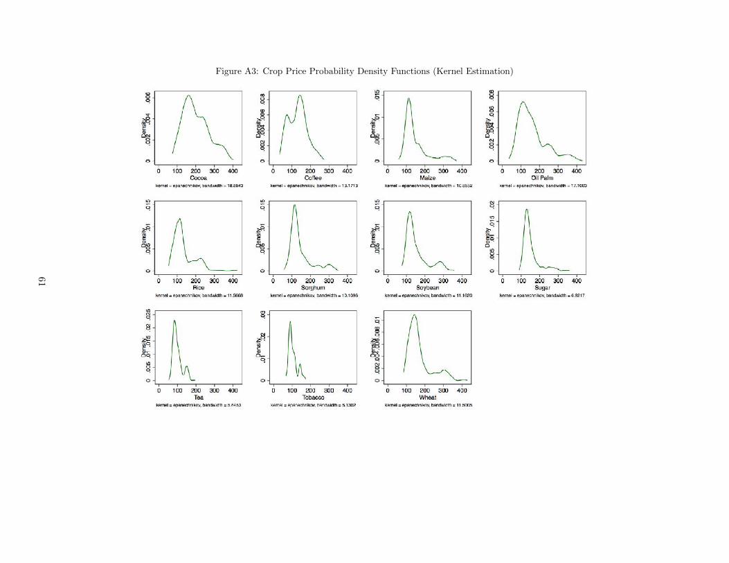
Figure A3: Crop Price Probability Density Functions (Kernel Estimation)

61

Figure A4: Crop Price Monthly Series (2000M01 = 100)

62

Appendix Tables

63

Table A1: Price Variables

Crop Description (from source) Source Consumer crop Producer crop

Bananas Central American and Ecuador, FOB U.S. Ports,US$ per metric ton

IMF Yes

Barley Canadian No.1 Western Barley, spot price, US$per metric ton

IMF Yes

Cocoa International Cocoa Organization cash price, CIFUS and European ports, US$ per metric ton

IMF Yes Yes (cash)

Coconut oil Philippines/Indonesia, bulk, c.i.f. Rotterdam,US$ per metric ton

WB Yes

Coffee 1 Robusta, International Coffee Organization NewYork cash price, ex-dock New York, US cents perpound

IMF Yes Yes (cash)

Coffee 2 Other Mild Arabicas, International Coffee Orga-nization New York cash price, ex-dock New York,US cents per pound

IMF Yes Yes (cash)

Maize U.S. No.2 Yellow, FOB Gulf of Mexico, U.S. price,US$ per metric ton

IMF Yes Yes (food)

Nuts Groundnuts (peanuts), 40/50 (40 to 50 count perounce), cif Argentina, US$ per metric ton

IMF Yes

Oil palm Malaysia Palm Oil Futures (first contract forward)4-5 percent FFA, US$ per metric ton

IMF Yes Yes (food)

Olive Olive Oil, extra virgin less than 1% free fatty acid,ex-tanker price U.K., US$ per metric ton

IMF Yes

Orange Miscellaneous oranges CIF French import price,US$ per metric ton

IMF Yes

Rice 5 percent broken milled white rice, Thailand nom-inal price quote, US$ per metric ton

IMF Yes Yes (food)

Sorghum Sorghum (US), no. 2 milo yellow, f.o.b. Gulf ports,US$ per metric ton

WB Yes Yes (food)

Soybean Chicago Soybean futures contract (first contractforward) No. 2 yellow and par, US$ per metricton

IMF Yes Yes (food)

Sugar 1 Free Market, Coffee Sugar and Cocoa Exchange(CSCE) contract no.11 nearest future position, UScents per pound

IMF Yes Yes (food)

Sugar 2 U.S. import price, contract no.14 nearest futuresposition, US cents per pound (Footnote: No. 14revised to No. 16)

IMF Yes Yes (food)

Sunflower Sunflower Oil, US export price from Gulf of Mex-ico, US$ per metric ton

IMF Yes

Tea Mombasa, Kenya, Auction Price, From July 1998,Kenya auctions, Best Pekoe Fannings. Prior, Lon-don auctions, c.i.f. U.K. warehouses, US cents perkilogram

IMF Yes Yes (cash)

Tobacco Any origin, unmanufactured, general import , cif,US$ per metric ton

WB No Yes (cash)

Wheat No.1 Hard Red Winter, ordinary protein, FOBGulf of Mexico, US$ per metric ton

IMF Yes Yes (food)

64

Table A2: UCDP Factor Conflict Results with Weather Covariates

Incidence1(Conflict > 0) 1(

OnsetConflict Begins)

Offset1(Conflict Ends)

(1) (2) (3) (4) (5) (6)

Producer Price Index -0.0050 -0.0048 -0.0024 -0.0021 0.0431 0.0302SE 0.002 0.002 0.001 0.001 0.017 0.012p-value 0.010 0.041 0.049 0.142 0.011 0.016

Consumer Price Index 0.0017 0.0011 -0.0690SE 0.001 0.001 0.030p-value 0.190 0.229 0.023

Temperature 0.0063 0.0093 0.0014 0.0051 -0.0222 0.0003SE 0.003 0.004 0.002 0.002 0.041 0.052p-value 0.060 0.038 0.509 0.036 0.590 0.995

Moderate drought -0.0036 -0.0027 -0.0014 -0.0023 0.0197 0.0169SE 0.005 0.005 0.003 0.003 0.064 0.061p-value 0.486 0.571 0.675 0.462 0.757 0.782

Severe drought 0.0058 0.0076 0.0022 0.0026 -0.1607 -0.1937SE 0.005 0.005 0.003 0.003 0.099 0.108p-value 0.217 0.096 0.438 0.353 0.107 0.075

Extreme drought -0.0028 0.0039 0.0003 0.0019 0.0600 -0.0283SE 0.004 0.004 0.003 0.002 0.056 0.052p-value 0.526 0.305 0.907 0.414 0.285 0.587

PPI impact (%) -18.4 -17.6 -16.9 -14.4 8.1 5.7CPI impact (%) 6.1 7.6 -12.9Wald test: PPI = CPI

p-value 0.000 0.002 0.010

Country × time trend Yes N/A Yes N/A Yes N/ACountry × year fixed effects No Yes No Yes No YesCell fixed effects Yes Yes Yes Yes Yes YesR squared 0.288 0.325 0.126 0.160 0.371 0.492Observations 204336 204336 201821 201821 4612 4479

Note: The dependent variables are UCDP Factor Conflict incidence, onset and offset dum-mies. The Producer Price Index (PPI) and Consumer Price Index (CPI) are measuredin terms of within-cell standard deviations. The coefficients displayed include two lags,i.e.,

∑2k=0 Price Indext−k. Standard errors allow for serial correlation within cells and

spatial correlation across cells within countries. PPI (CPI) impact indicates the effectof a one standard deviation rise in producer (consumer) prices on the outcome variablein percentage terms. Temperature is the cell-year mean temperature in degrees celsius;moderate drought indicates that there were at least three consecutive months in whichrainfall was more than 1 standard deviation below long term (six-month) levels; severedrought indicates that there were at least two months during which rainfall was morethan 1.5 standard deviations below long term levels; and extreme drought indicates thatboth of these criteria were met in a cell-year.

65

Table A3: UCDP Factor Conflict Results with Weather Covariates, Conley SEs

UCDP Factor Conflict:Incidence

1(Conflict > 0) 1(Onset

Conflict Begins)Offset

1(Conflict Ends)

(1) (2) (3) (4) (5) (6)

Producer Price Index -0.0050 -0.0048 -0.0024 -0.0021 0.0431 0.0302Conley SE 0.001 0.001 0.001 0.001 0.011 0.008p-value 0.000 0.000 0.002 0.020 0.000 0.000

Consumer Price Index 0.0017 0.0011 -0.0690Conley SE 0.001 0.000 0.018p-value 0.014 0.021 0.000

Temperature 0.0063 0.0093 0.0014 0.0051 -0.0222 0.0003Conley SE 0.002 0.002 0.001 0.002 0.028 0.042p-value 0.000 0.000 0.242 0.001 0.420 0.994

Moderate drought -0.0036 -0.0027 -0.0014 -0.0023 0.0197 0.0169Conley SE 0.004 0.003 0.003 0.003 0.062 0.056p-value 0.337 0.436 0.604 0.374 0.752 0.762

Severe drought 0.0058 0.0076 0.0022 0.0026 -0.1607 -0.1937Conley SE 0.003 0.003 0.002 0.002 0.096 0.095p-value 0.081 0.018 0.344 0.261 0.093 0.041

Extreme drought -0.0028 0.0039 0.0003 0.0019 0.0600 -0.0283Conley SE 0.003 0.003 0.002 0.002 0.047 0.045p-value 0.365 0.170 0.871 0.333 0.199 0.531

PPI impact (%) -18.4 -17.6 -16.9 -14.4 8.1 5.7CPI impact (%) 6.1 7.6 -12.9Wald test: PPI = CPI

p-value 0.002 0.001 0.005

Country × time trend Yes N/A Yes N/A Yes N/ACountry × year fixed effects No Yes No Yes No YesCell fixed effects Yes Yes Yes Yes Yes YesR squared 0.288 0.325 0.126 0.160 0.453 0.572Observations 204336 204336 201822 201822 5329 5329

Note: The dependent variables are UCDP Factor Conflict incidence, onset and offset dum-mies. The Producer Price Index (PPI) and Consumer Price Index (CPI) are measuredin terms of within-cell standard deviations. The coefficients displayed include two lags,i.e.,

∑2k=0 Price Indext−k. Standard errors allow for serial and spatial correlation in

groups of contiguous cells. PPI (CPI) impact indicates the effect of a one standard de-viation rise in producer (consumer) prices on the outcome variable in percentage terms.Temperature is the cell-year mean temperature in degrees celsius; moderate drought in-dicates that there were at least three consecutive months in which rainfall was morethan 1 standard deviation below long term (six-month) levels; severe drought indicatesthat there were at least two months during which rainfall was more than 1.5 standarddeviations below long term levels; and extreme drought indicates that both of these cri-teria were met in a cell-year.

66

Table A4: UCDP Factor Conflict Results with Oil Covariates

Incidence1(Conflict > 0) 1(

OnsetConflict Begins)

Offset1(Conflict Ends)

(1) (2) (3) (4) (5) (6)

Producer Price Index -0.0052 -0.0048 -0.0024 -0.0021 0.0348 0.0301SE 0.002 0.002 0.001 0.001 0.015 0.012p-value 0.011 0.046 0.058 0.152 0.018 0.013

Consumer Price Index 0.0017 0.0033 -0.0238SE 0.002 0.002 0.040p-value 0.473 0.059 0.551

Oil price × oil cell 0.0000 0.0000 0.0000 -0.0000 -0.0007 -0.0006SE 0.000 0.000 0.000 0.000 0.000 0.001p-value 0.635 0.666 0.972 0.892 0.106 0.263

Oil price × oil country -0.0001 -0.0001 0.0004SE 0.000 0.000 0.001p-value 0.034 0.048 0.537

Oil price 0.0075 0.0022 -0.0600SE 0.004 0.003 0.046p-value 0.050 0.423 0.190

PPI impact (%) -19.3 -17.9 -16.9 -14.3 6.5 5.6CPI impact (%) 6.3 22.6 -4.5Wald test: PPI = CPI

p-value 0.007 0.000 0.235

Country × time trend Yes N/A Yes N/A Yes N/ACountry × year fixed effects No Yes No Yes No YesCell fixed effects Yes Yes Yes Yes Yes YesR squared 0.288 0.325 0.126 0.160 0.380 0.493Observations 204666 204666 202151 202151 4614 4479

Note: The dependent variables are UCDP Factor Conflict incidence, onset and offset dum-mies. The Producer Price Index (PPI) and Consumer Price Index (CPI) are measuredin terms of within-cell standard deviations. The coefficients displayed include two lags,i.e.,

∑2k=0 Price Indext−k. Standard errors allow for serial correlation within cells and

spatial correlation across cells within countries. PPI (CPI) impact indicates the effectof a one standard deviation rise in producer (consumer) prices on the outcome variablein percentage terms. Oil cell is a dummy indicating the presence of an oil field in a givencell, and oil country is a dummy indicating that there is an oil field in the given country.

67

Table A5: Alternative Factor Conflict Comparisons

Incidence 1(Conflict > 0)

(1) (2) (3)

Producer Price Index -0.0003 -0.0012 -0.0068SE 0.000 0.001 0.002p-value 0.540 0.098 0.003

Consumer Price Index 0.0004 0.0000 -0.0003SE 0.000 0.000 0.001p-value 0.169 0.874 0.835

PPI impact (%) -6.5 -28.0 -25.3CPI impact (%) 8.8 1.1 -1.0Wald test: PPI = CPI

p-value 0.154 0.083 0.002

Country × time trend Yes Yes YesCell fixed effects Yes Yes YesSample 1997-2013 1997-2010 1997-2010Dep. Var. Territory Territory FactorSource ACLED ACLED UCDPR squared 0.115 0.139 0.359Observations 158151 130242 130242

Note: The dependent variable Territory is taken from theACLED project, and is equal to 1 if a battle takes place inwhich territorial control is transferred. The dependent vari-able Factor is UCDP Factor Conflict. The Producer PriceIndex (PPI) and Consumer Price Index (CPI) are measuredin terms of within-cell standard deviations. The coefficientsdisplayed include two lags, i.e.,

∑2k=0 Price Indext−k. Stan-

dard errors allow for serial correlation within cells and spa-tial correlation across cells within countries. PPI (CPI)impact indicates the effect of a within-cell one standard de-viation rise in producer (consumer) prices on the outcomevariable in percentage terms.

68

Table A6: UCDP Factor Conflict: 1 Degree Aggregation with Spatially Lagged PPI

UCDP Factor Conflict:Incidence

1(Conflict > 0) 1(Onset

Conflict Begins)Offset

1(Conflict Ends)

(1) (2) (3) (4) (5) (6)

Producer Price Index -0.0039 -0.0054 -0.0007 -0.0016 0.0205 0.0250Conley SE 0.002 0.002 0.002 0.002 0.014 0.012

p-value 0.069 0.010 0.718 0.388 0.146 0.042Clustered SE 0.003 0.003 0.002 0.002 0.016 0.013

p-value 0.194 0.072 0.717 0.397 0.212 0.057

Producer Price Index × W -0.0001 -0.0021 -0.0021 -0.0024 0.0090 0.0030Conley SE 0.003 0.003 0.002 0.003 0.015 0.016

p-value 0.979 0.958 0.409 0.354 0.557 0.849Clustered SE 0.004 0.005 0.003 0.004 0.018 0.017

p-value 0.984 0.974 0.486 0.503 0.621 0.859

Consumer Price Index -0.0019 0.0005 -0.0810Conley SE 0.001 0.001 0.020

p-value 0.138 0.625 0.000Clustered SE 0.002 0.002 0.027

p-value 0.449 0.785 0.003

PPI impact (%) -5.4 -7.6 -1.5 -3.6 3.2 3.9PPI ×W impact (%) -0.1 0.2 -4.6 -5.4 1.4 0.5CPI impact (%) -2.6 1.1 -12.7Wald test: PPI = CPI

p-value 0.639 0.642 0.004

Country × time trend Yes N/A Yes N/A Yes N/ACountry × year fixed effects No Yes No Yes No YesCell fixed effects Yes Yes Yes Yes Yes YesR squared 0.325 0.411 0.170 0.249 0.280 0.431Observations 54010 53968 53887 53843 3571 3417

Note: The dependent variables are UCDP Factor Conflict incidence, onset and offset dum-mies. The Producer Price Index (PPI) and Consumer Price Index (CPI) are measuredin terms of within-cell standard deviations. The coefficients displayed include two lags,i.e.,

∑2k=0 Price Indext−k. Conley standard errors allow for serial and spatial correla-

tion in groups of contiguous cells. Clustered standard errors allow for serial correlationwithin cells and spatial correlation across cells within countries. PPI (CPI) impact in-dicates the effect of a one standard deviation rise in producer (consumer) prices on theoutcome variable in percentage terms. W is a spatial weighting matrix; the spatial lagPPI ×W measures the PPI in all eight neighboring cells.

69

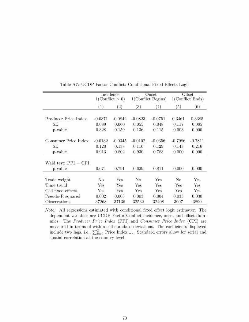
Table A7: UCDP Factor Conflict: Conditional Fixed Effects Logit

Incidence1(Conflict > 0) 1(

OnsetConflict Begins)

Offset1(Conflict Ends)

(1) (2) (3) (4) (5) (6)

Producer Price Index -0.0871 -0.0842 -0.0823 -0.0751 0.3461 0.3385SE 0.089 0.060 0.055 0.048 0.117 0.085p-value 0.328 0.159 0.136 0.115 0.003 0.000

Consumer Price Index -0.0132 -0.0345 -0.0102 -0.0356 -0.7986 -0.7811SE 0.120 0.138 0.116 0.129 0.143 0.216p-value 0.913 0.802 0.930 0.783 0.000 0.000

Wald test: PPI = CPIp-value 0.671 0.791 0.629 0.811 0.000 0.000

Trade weight No Yes No Yes No YesTime trend Yes Yes Yes Yes Yes YesCell fixed effects Yes Yes Yes Yes Yes YesPseudo-R squared 0.002 0.003 0.003 0.004 0.033 0.030Observations 37268 37136 32532 32408 3907 3890

Note: All regressions estimated with conditional fixed effect logit estimator. Thedependent variables are UCDP Factor Conflict incidence, onset and offset dum-mies. The Producer Price Index (PPI) and Consumer Price Index (CPI) aremeasured in terms of within-cell standard deviations. The coefficients displayedinclude two lags, i.e.,

∑2k=0 Price Indext−k. Standard errors allow for serial and

spatial correlation at the country level.

70

Table A8: ACLED Output Conflict and Disaggregated Producer Prices

ACLED Output Conflict:Incidence

1(Conflict > 0) 1(Onset

Conflict Begins)Offset

1(Conflict Ends)

(1) (2) (3) (4) (5) (6)

Producer Price Index: Food crops 0.0083 0.0077 0.0072 0.0062 0.0076 0.0092Conley SE 0.001 0.001 0.001 0.001 0.002 0.002

p-value 0.000 0.000 0.000 0.000 0.001 0.000Clustered SE 0.003 0.002 0.002 0.002 0.004 0.004

p-value 0.001 0.002 0.000 0.001 0.061 0.026

Producer Price Index: Cash crops -0.0026 -0.0019 -0.0014 -0.0008 0.0118 0.0160Conley SE 0.001 0.001 0.001 0.001 0.004 0.004

p-value 0.023 0.123 0.223 0.491 0.001 0.000Clustered SE 0.002 0.002 0.002 0.002 0.007 0.008

p-value 0.225 0.404 0.461 0.676 0.082 0.043

PPI Impact: Food crops 16.6 15.3 25.5 21.9 1.7 2.0PPI Impact: Cash crops -5.2 -3.7 -5.0 -2.9 2.6 3.5Wald test: PPI Food = PPI Cash

p-value 0.000 0.002 0.000 0.004 0.522 0.370

Trade weight No Yes No Yes No YesCountry × year fixed effects Yes Yes Yes Yes Yes YesCell FE Yes Yes Yes Yes Yes YesR squared 0.399 0.397 0.195 0.196 0.545 0.550Observations 173876 158151 169933 154677 7410 6625

Note: The dependent variables are ACLED Output Conflict incidence, onset and offset dum-mies. The Producer Price Index (PPI) variables are measured in terms of within-cell standarddeviations. Food crops are crops that each represent at least 1% of caloric intake in the sam-ple; cash crops are the rest (see Table A1). The coefficients displayed include two lags, i.e.,∑2

k=0 Price Indext−k. Conley standard errors allow for serial and spatial correlation in groupsof contiguous cells. Clustered standard errors allow for serial correlation within cells and spa-tial correlation across cells within countries. PPI Impact indicates the effect of a within-cellone standard deviation rise in producer prices on the outcome variable in percentage terms.

71

Table A9: ACLED Output Conflict, Producer Prices and Consumer Prices: with WeatherCovariates

ACLED Output Conflict:Incidence

1(Conflict > 0) 1(Onset

Conflict Begins)Offset

1(Conflict Ends)

(1) (2) (3) (4) (5) (6)

Producer Price Index: Food crops 0.0084 0.0077 0.0065 0.0062 0.0079 0.0090SE 0.002 0.002 0.002 0.002 0.005 0.004p-value 0.000 0.002 0.000 0.001 0.110 0.028

Producer Price Index: Cash crops -0.0008 -0.0018 -0.0001 -0.0008 0.0099 0.0165SE 0.002 0.002 0.002 0.002 0.008 0.008p-value 0.695 0.426 0.937 0.695 0.190 0.037

Consumer Price Index 0.0038 0.0018 -0.0960SE 0.001 0.001 0.018p-value 0.001 0.016 0.000

Temperature -0.0143 0.0063 -0.0070 0.0050 0.1436 0.0600SE 0.005 0.005 0.003 0.003 0.036 0.045p-value 0.002 0.181 0.046 0.150 0.000 0.185

Moderate drought 0.0218 0.0152 0.0140 0.0080 -0.0932 -0.0487SE 0.007 0.007 0.005 0.005 0.065 0.067p-value 0.001 0.020 0.007 0.100 0.149 0.470

Severe drought 0.0008 -0.0051 0.0018 -0.0031 -0.0345 0.1210SE 0.005 0.005 0.004 0.004 0.092 0.103p-value 0.872 0.310 0.654 0.417 0.707 0.242

Extreme drought 0.0099 0.0024 0.0118 0.0049 -0.0351 -0.0246SE 0.007 0.006 0.005 0.005 0.065 0.069p-value 0.155 0.696 0.028 0.303 0.589 0.722

PPI impact: Food crops (%) 16.6 15.3 22.8 21.9 1.7 2.0PPI impact: Cash crops (%) -1.6 -3.5 -0.5 -2.8 2.2 3.6CPI impact (%) 7.6 6.5 -21.3Wald test: PPI Food = PPI Cash

p-value 0.003 0.002 0.005 0.004 0.763 0.325

Country × time trend Yes N/a Yes N/a Yes N/aCountry × year fixed effects No Yes No Yes No YesCell FE Yes Yes Yes Yes Yes YesR squared 0.372 0.397 0.167 0.197 0.442 0.551Observations 157896 157896 154424 154424 6760 6618

Note: The dependent variables are ACLED Output Conflict incidence, onset and offset dummies.The Producer Price Index (PPI) and Consumer Price Index (CPI) variables are measured interms of within-cell standard deviations. Food crops are crops that each represent at least 1%of caloric intake in the sample; cash crops are the rest (see Table A1). The coefficients dis-

played include two lags, i.e.,∑2

k=0 Price Indext−k. Standard errors allow for serial correlationwithin cells and spatial correlation across cells within countries. PPI (CPI) Impact indicatesthe effect of a one standard deviation rise in producer (consumer) prices on the outcome vari-able in percentage terms. Temperature is the cell-year mean temperature in degrees celsius;moderate drought indicates that there were at least three consecutive months in which rainfallwas more than 1 standard deviation below long term (six-month) levels; severe drought indi-cates that there were at least two months during which rainfall was more than 1.5 standarddeviations below long term levels; and extreme drought indicates that both of these criteriawere met in a cell-year.

72

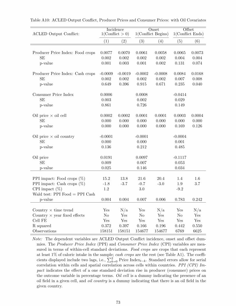
Table A10: ACLED Output Conflict, Producer Prices and Consumer Prices: with Oil Covariates

ACLED Output Conflict:Incidence

1(Conflict > 0) 1(Onset

Conflict Begins)Offset

1(Conflict Ends)

(1) (2) (3) (4) (5) (6)

Producer Price Index: Food crops 0.0077 0.0070 0.0061 0.0058 0.0065 0.0073SE 0.002 0.002 0.002 0.002 0.004 0.004p-value 0.001 0.003 0.001 0.002 0.131 0.074

Producer Price Index: Cash crops -0.0009 -0.0019 -0.0002 -0.0008 0.0084 0.0168SE 0.002 0.002 0.002 0.002 0.007 0.008p-value 0.649 0.396 0.915 0.671 0.235 0.040

Consumer Price Index 0.0006 0.0008 -0.0414SE 0.003 0.002 0.029p-value 0.861 0.726 0.149

Oil price × oil cell 0.0002 0.0002 0.0001 0.0001 0.0003 0.0004SE 0.000 0.000 0.000 0.000 0.000 0.000p-value 0.000 0.000 0.000 0.000 0.169 0.126

Oil price × oil country -0.0001 -0.0001 -0.0004SE 0.000 0.000 0.001p-value 0.136 0.212 0.485

Oil price 0.0191 0.0097 -0.1117SE 0.009 0.007 0.053p-value 0.025 0.146 0.034

PPI impact: Food crops (%) 15.2 13.8 21.6 20.4 1.4 1.6PPI impact: Cash crops (%) -1.8 -3.7 -0.7 -3.0 1.9 3.7CPI impact (%) 1.2 3.0 -9.2Wald test: PPI Food = PPI Cash

p-value 0.004 0.004 0.007 0.006 0.783 0.242

Country × time trend Yes N/a Yes N/a Yes N/aCountry × year fixed effects No Yes No Yes No YesCell FE Yes Yes Yes Yes Yes YesR squared 0.372 0.397 0.166 0.196 0.442 0.550Observations 158151 158151 154677 154677 6769 6625

Note: The dependent variables are ACLED Output Conflict incidence, onset and offset dum-mies. The Producer Price Index (PPI) and Consumer Price Index (CPI) variables are mea-sured in terms of within-cell standard deviations. Food crops are crops that each representat least 1% of caloric intake in the sample; cash crops are the rest (see Table A1). The coeffi-cients displayed include two lags, i.e.,

∑2k=0 Price Indext−k. Standard errors allow for serial

correlation within cells and spatial correlation across cells within countries. PPI (CPI) Im-pact indicates the effect of a one standard deviation rise in producer (consumer) prices onthe outcome variable in percentage terms. Oil cell is a dummy indicating the presence of anoil field in a given cell, and oil country is a dummy indicating that there is an oil field in thegiven country.

73

Table A11: ACLED Output Conflict: 1 Degree Aggregation with Spatially Lagged PPI

Incidence1(Conflict > 0) 1(

OnsetConflict Begins)

Offset1(Conflict Ends)

(1) (2) (3) (4) (5) (6)

Producer Price Index: Food crops 0.0060 0.0066 0.0107 0.0113 0.0035 -0.0024Conley SE 0.004 0.003 0.004 0.003 0.005 0.004

p-value 0.093 0.013 0.003 0.000 0.493 0.539Clustered SE 0.004 0.004 0.003 0.003 0.006 0.006

p-value 0.174 0.119 0.001 0.000 0.533 0.683

Producer Price Index: Cash crops -0.0106 -0.0127 -0.0090 -0.0109 0.0183 0.0152Conley SE 0.005 0.004 0.004 0.004 0.007 0.008

p-value 0.019 0.001 0.034 0.007 0.009 0.059Clustered SE 0.004 0.004 0.004 0.005 0.008 0.009

p-value 0.011 0.004 0.042 0.017 0.029 0.105

Producer Price Index: Food crops ×W 0.0090 0.0007 0.0058 -0.0002 0.0193 0.0273Conley SE 0.004 0.003 0.004 0.003 0.009 0.006

p-value 0.022 0.804 0.135 0.943 0.031 0.000Clustered SE 0.005 0.005 0.005 0.005 0.014 0.011

p-value 0.078 0.885 0.254 0.961 0.156 0.011

Producer Price Index: Cash crops ×W 0.0159 0.0010 0.0158 0.0031 -0.0211 -0.0129Conley SE 0.005 0.005 0.005 0.005 0.008 0.012

p-value 0.001 0.845 0.001 0.554 0.009 0.282Clustered SE 0.005 0.008 0.006 0.007 0.013 0.015

p-value 0.002 0.901 0.005 0.647 0.105 0.389

Consumer Price Index 0.0255 0.0162 -0.1769Conley SE 0.002 0.001 0.012

p-value 0.000 0.000 0.000Clustered SE 0.004 0.003 0.021

p-value 0.000 0.000 0.000

PPI impact: Food crops (%) 4.3 4.8 12.0 12.6 0.6 -0.4PPI impact: Cash crops (%) -7.7 -9.2 -10.1 -12.2 3.3 2.8PPI × W impact: Food crops (%) 6.5 0.5 6.5 -0.3 3.5 5.0PPI × W impact: Cash crops (%) 11.6 0.7 17.7 3.5 -3.8 -2.4CPI impact (%) 18.5 18.1 -32.3Wald test: PPI Food = PPI Cash

p-value 0.008 0.003 0.001 0.000 0.157 0.136

Country × time trend Yes N/a Yes N/a Yes N/aCountry × year fixed effects No Yes No Yes No YesCell fixed effects Yes Yes Yes Yes Yes YesR squared 0.417 0.488 0.207 0.284 0.313 0.495Observations 41735 41701 41644 41608 5407 5240

Note: The dependent variables are ACLED Output Conflict incidence, onset and offset dummies.The Producer Price Index (PPI) and Consumer Price Index (CPI) variables are measured in termsof within-cell standard deviations. Food crops are crops that each represent at least 1% of caloricintake in the sample; cash crops are the rest (see Table A1). The coefficients displayed include two

lags, i.e.,∑2

k=0 Price Indext−k. Standard errors allow for serial correlation within cells and spatialcorrelation across cells within countries. PPI (CPI) Impact indicates the effect of a one standarddeviation rise in producer (consumer) prices on the outcome variable in percentage terms. W is aspatial weighting matrix; the spatial lag PPI ×W measures the PPI in all eight neighboring cells.

74

Table A12: ACLED Output Conflict: Conditional Fixed Effects Logit

Incidence1(Conflict > 0) 1(

OnsetConflict Begins)

Offset1(Conflict Ends)

(1) (2) (3) (4) (5) (6)

Producer Price Index: Food crops 0.0292 -0.0085 0.0304 0.0068 -0.0000 0.0486SE 0.020 0.045 0.019 0.039 0.016 0.036p-value 0.139 0.849 0.107 0.860 0.998 0.179

Producer Price Index: Cash crops -0.0221 -0.0084 -0.0161 -0.0098 0.0492 0.0274SE 0.021 0.026 0.019 0.022 0.020 0.034p-value 0.301 0.749 0.394 0.655 0.013 0.420

Consumer Price Index 0.3646 0.2601 0.1572 0.0906 -0.6686 -0.5787SE 0.150 0.161 0.106 0.119 0.170 0.208p-value 0.015 0.105 0.138 0.447 0.000 0.005

Wald test: PPI = CPIp-value 0.073 0.999 0.114 0.764 0.035 0.714

Trade weight No Yes No Yes No YesTime trend Yes Yes Yes Yes Yes YesCell fixed effects Yes Yes Yes Yes Yes YesPseudo-R squared 0.063 0.055 0.058 0.055 0.148 0.133Observations 42092 42058 37870 37837 5462 5457

Note: All regressions estimated with conditional fixed effect logit estimator. The dependentvariables are ACLED Output Conflict incidence, onset and offset dummies. The ProducerPrice Index (PPI) and Consumer Price Index (CPI) variables are measured in terms ofwithin-cell standard deviations. The coefficients displayed include two lags, i.e.,

∑2k=0 Price

Indext−k. Standard errors allow for serial and spatial correlation at the country level.

75

Table A13: ACLED Output Conflict, Producer Prices and Consumer Prices: UrbanRiots

ACLED Output Conflict: Incidence: 1(Conflict > 0)

(1) (2) (3) (4)

Producer Price Index: Food crops 0.0036 0.0029 0.0078 0.0071SE 0.002 0.002 0.002 0.003p-value 0.088 0.175 0.002 0.005

Producer Price Index: Cash crops -0.0003 -0.0015 -0.0006 -0.0018SE 0.002 0.002 0.002 0.002p-value 0.898 0.497 0.761 0.407

Consumer Price Index 0.0023 0.0039SE 0.001 0.001p-value 0.032 0.001

Consumer Price Index × urban area 0.2071 0.2038SE 0.049 0.048p-value 0.000 0.000

Consumer Price Index × urban population 0.0000 0.0000SE 0.000 0.000p-value 0.384 0.378

CPI impact (%) at urban area = 0 4.6CPI impact (%) at urban area 90th pctile 12.0 7.3

CPI impact (%) at urban pop = 0 7.8CPI impact (%) at urban pop 90th pctile 8.2 0.4

Country × time trend Yes N/a Yes N/aCountry × year fixed effects No Yes No YesCell FE Yes Yes Yes YesR squared 0.373 0.399 0.371 0.397Observations 158049 158049 158151 158151

Note: The dependent variables are ACLED Output Conflict incidence, onset andoffset dummies. The Producer Price Index (PPI) and Consumer Price Index(CPI) variables are measured in terms of within-cell standard deviations. Foodcrops are crops that each represent at least 1% of caloric intake in the sample;cash crops are the rest (see Table A1). The coefficients displayed include two lags,i.e.,

∑2k=0 Price Indext−k. Standard errors allow for serial correlation within cells

and spatial correlation across cells within countries. PPI (CPI) Impact indicatesthe effect of one within-cell standard deviation rise in producer (consumer) priceson the outcome variable in percentage terms. Urban area is the percentage of agiven cell area classified as urban; urban population is the percentage of a givencell’s population classified as living in urban areas.

76

Table A14: Comparison of Effects on Output Conflict and Factor Conflict Incidence

ACLEDOutput Conflict

ACLEDTerritorial Change

UCDPFactor Conflict

(1) (2) (3) (4) (5) (6)

Producer Price Index: Food crops 0.0084 0.0017 0.0002 -0.0001 -0.0042 -0.0058SE 0.002 0.003 0.000 0.000 0.002 0.002p-value 0.000 0.519 0.256 0.242 0.041 0.017

Producer Price Index: Cash crops -0.0006 0.0013 -0.0008 -0.0030 -0.0025 -0.0040SE 0.002 0.003 0.001 0.002 0.002 0.002p-value 0.753 0.653 0.312 0.055 0.110 0.049

Consumer Price Index 0.0040 -0.0001 0.0003 0.0000 0.0016 -0.0003SE 0.001 0.001 0.000 0.000 0.001 0.001p-value 0.001 0.921 0.226 0.986 0.206 0.826

PPI Impact: Food crops 16.6 3.4 4.9 -2.9 -15.6 -21.3PPI Impact: Cash crops -1.2 2.6 -19.6 -71.7 -9.4 -14.6CPI impact (%) 7.9 -0.2 7.9 0.1 5.9 -1.0Wald test: PPI (total) = CPI

p-value 0.260 0.437 0.218 0.037 0.000 0.000Wald test: PPI Food = PPI Cash

p-value 0.003 0.925 0.229 0.067 0.547 0.599

Sample 1997-2013 1997-2010 1997-2013 1997-2010 1989-2010 1997-2010Country × time trend Yes Yes Yes Yes Yes YesCell fixed effects Yes Yes Yes Yes Yes YesR squared 0.371 0.395 0.115 0.140 0.288 0.359Observations 158151 130242 158151 130242 204666 130242

Note: All three dependent variables measure conflict incidence: 1(Conflict > 0). The dependent variableTerritorial Change is taken from the ACLED project, and is equal to 1 if a battle takes place in which ter-ritorial control is transferred. The Producer Price Index (PPI) and Consumer Price Index (CPI) variablesare measured in terms of within-cell standard deviations. Food crops are crops that each represent at least1% of caloric intake in the sample; cash crops are the rest (see Table A1). The coefficients displayed in-clude two lags, i.e.,

∑2k=0 Price Indext−k. Standard errors allow for serial correlation within cells and spatial

correlation across cells within countries. PPI (CPI) Impact indicates the effect of one within-cell standarddeviation rise in producer (consumer) prices on the outcome variable in percentage terms.

77

Table A15: Afrobarometer: Prices and Poverty

Poverty: index Poverty: income Poverty: food

(1) (2) (3) (4) (5) (6) (7) (8) (9)

Producer Price Index -0.0004 0.0011 0.0094 -0.0022 -0.0021 0.0036 -0.0049 -0.0015 0.0059SE 0.002 0.004 0.007 0.002 0.002 0.005 0.002 0.003 0.006p-value 0.878 0.766 0.191 0.197 0.382 0.471 0.020 0.619 0.284

Producer Price Index × farmer -0.0046 -0.0048 -0.0007 -0.0013 -0.0029 -0.0040SE 0.002 0.002 0.002 0.001 0.002 0.002p-value 0.023 0.010 0.648 0.375 0.160 0.054

Consumer Price Index 0.0552 0.0531 0.0599SE 0.033 0.021 0.027p-value 0.091 0.014 0.029

PPI impact (%) -0.1 0.2 2.1 -0.4 -0.3 0.6 -1.4 -0.4 1.7PPI impact × farmer (%) -1.0 -1.1 -0.1 -0.2 -0.8 -1.1CPI impact (%) 12.2 8.6 17.4

Country × time trend Yes N/a N/a Yes N/a N/a Yes N/a N/aCountry × period fixed effects No Yes Yes No Yes Yes No Yes YesControls Yes Yes Yes Yes Yes Yes Yes Yes YesArea FE Country Country Cell Country Country Cell Country Country CellSurvey round fixed effects Yes Yes Yes Yes Yes Yes Yes Yes YesR squared 0.130 0.156 0.202 0.145 0.148 0.180 0.107 0.119 0.160Observations 66946 41133 41121 66543 40860 40848 66836 41059 41047

Note: The dependent variables as follows: Poverty: index indicates that a household has an above-median score on a 25-pointpoverty index that measures access to food, water, health, electricity and income; Poverty: income indicates that a householdhas frequently gone without income over the preceding year; Poverty: food indicates that a household has frequently gone with-out food over the preceding year. Columns (1), (4) and (6) have larger sample sizes as data on occupation is not available inall rounds. The Producer Price Index (PPI) and Consumer Price Index (CPI) variables are measured in terms of within-cellstandard deviations. Food crops are crops that each represent at least 1% of caloric intake in the sample; cash crops are therest (see Table A1). The coefficients displayed include four lags, i.e.,

∑4k=0 Price Indext−k, where each t is a six-month period.

Standard errors allow for serial and spatial correlation within cells. PPI (CPI) Impact indicates the effect of one within-cellstandard deviation rise in producer (consumer) prices on the outcome variable in percentage terms.

78

Table A16: Afrobarometer: Output Conflict Validation Tests

Theft Violence Protest

(1) (2) (3) (4) (5) (6) (7) (8) (9)

ACLED Output Conflict 0.0758 0.0447 0.0428 0.0594 0.0251 0.0223 0.0106 0.0166 0.0167SE 0.012 0.011 0.012 0.010 0.007 0.007 0.009 0.007 0.007p-value 0.000 0.000 0.000 0.000 0.000 0.001 0.252 0.013 0.014

UCDP Factor Conflict 0.0104 0.0165 -0.0027SE 0.022 0.021 0.016p-value 0.641 0.437 0.867

ACLED Output Conflict (%) 24.2 14.3 13.7 45.4 19.2 17.1 7.8 12.2 12.2UCDP Factor Conflict (%) 3.3 12.6 -2.0

Country fixed effects No Yes Yes No Yes Yes No Yes YesSurvey round fixed effects No Yes Yes No Yes Yes No Yes YesR squared 0.006 0.021 0.022 0.006 0.023 0.024 0.000 0.021 0.021Observations 67500 67500 67500 67533 67533 67533 67028 67028 67028

Note: The dependent variables are binary responses to survey questions that ask whether individuals over theprevious year (i) have been victims of theft; (ii) have been victims of physical assault; (iii) have partaken in“protest marches”. The coefficients displayed include lags that cover the previous year, i.e.,

∑2k=0 Conflictt−k,

where each t is a six-month period. Standard errors allow for serial and spatial correlation within cells.

79