The Economic Stimulus Payments of 2008 and the Aggregate Demand for Consumption*

Christian Broda Duquesne Capital Management and NBER Jonathan A. Parker Northwestern University and NBER

Working draft, December 2012 Abstract: This paper uses the randomized timing of the disbursement of the Economic Stimulus Payments (ESPs) of 2008 and a supplemental survey of households in the Nielsen Consumer Panel to estimate the causal effect of the receipt of an ESP on measured household spending. Household spending rises by ten percent the week of receipt, and roughly four percent during the two months during and following receipt. Spending effects are large and significant only for households without high past income or without adequate liquid wealth. Among households that knew the amount of their ESP prior to receipt, there are no significant increases in spending at the different times that households report learning the amount. These results and the timing of disbursements imply a partial-equilibrium increase in aggregate demand caused by the distribution of ESPs that is significant in the second quarter of 2008 and statistically weak but still economically significant in the third quarter.

* We thank the Kellogg School of Management at Northwestern University, the Initiative for Global Markets at the University of Chicago, and the Zell Center at the Kellogg School of Management for funding. Parker thanks the Laboratory for Applied Economics and Policy at Harvard for funding. For helpful comments on our research, we thank: Jordi Gali, Greg Kaplan, Nicholas Souleles, two anonymous referees on our grant application; participants at seminars at the Board of Governors of the Federal Reserve System, and Harvard; and participants at the Journal of Monetary Economics – Swiss National Bank – Study Center Gerzensee Conference, October 2012. We would also like to thank Ed Grove, Matt Knain and Molly Hagen at ACNielsen for their careful explanation of the ACNielsen Homescan survey and the data. The results contained in this paper do not reflect the views of AC Nielsen. This paper replaces the earlier analysis in Broda and Parker (2008). Contact author Parker: Kellogg School of Management, Northwestern University, http://www.kellogg.northwestern.edu/ faculty/parker/htm/

1

Early in 2008, in response to slowing economic growth, the Federal government passed the

Economic Stimulus Act (ESA) of 2008. A combination of $100 billion in tax rebates and $50 billion

in business investment incentives, the Act was designed to increase demand for investment and

consumption goods and services, and so raise national output and combat the recession that began in

December 2007. The tax rebates, called economic stimulus payments (ESPs), averaged just under

$1000 per recipient and were sent to 130 million U.S. tax filers in the spring and summer of 2008.

This paper asks whether the receipt of the ESPs in 2008 caused households to increase their spending.

On the one hand, around the time of the ESP program measured aggregate consumption is

relatively smooth while measured disposable income rises and falls sharply with the disbursement of

ESPs, providing “no evidence that the stimulus has had any impact in raising consumption” (Taylor

(2010); see also Feldstein (2008)). And according to the theory typically embedded in most

macroeconomic models used to study the effects of fiscal stabilization policy – the textbook rational

expectations Life-cycle/Permanent-income Hypothesis (LCPIH) – the arrival of a predictable ESP

should cause no change in spending.

On the other hand, the majority of previous research finds that consumption expenditures rise

in response to predictable, predetermined and plausibly-exogenous changes in household-level

income.1 Most immediately relevant, Johnson, Parker, and Souleles (2006), Agarwal, Lui, and

Souleles (2007), and Johnson, Parker, and Souleles (2009) all find significant spending responses to

the receipt of previous Federal tax rebates. Households when surveyed about what they would do or

have done with tax rebates report spending a significant fraction (Shapiro and Slemrod (1995 and

2003) and Coronado, Lupton, and Sheiner (2006)). And significant spending responses are consistent

with a number of alternative theories, such those in which households are impatient and face financial

frictions, in which households have limited attention, or in which households use mental accounts.

In this paper, we follow the Johnson, Parker, and Souleles (2006) methodology and measure

the effect of the receipt of the ESPs of 2008 on the demand for consumption by measuring the change

in the timing of the spending of a household caused by the timing of the receipt of its ESP, and then

aggregating these changes using the temporal distribution of ESPs as reported by the U.S. Treasury

1See for example Jonathan A. Parker (1999), Nicholas S. Souleles (1999, 2002), and Chang-Tai Hsieh (2003), or the reviews of Deaton (1992), Browning and Lusardi (1996), Johnson, Parker, and Souleles (2006), and Jappelli and Pistaferri (2010).

2

and several different extrapolations from the goods we observe to a broader measure of spending.

We emphasize ‘receipt’ because we do not measure the impact of any change in spending that is

uncorrelated with the time of receipt, such as increase in spending on the date of announcement or

reduced spending in the future uncorrelated with receipt. We emphasize ‘demand’ because the

calculation is purely partial equilibrium and omits any multiplier or crowding-out effects of the policy

(although our findings are useful for modeling and understanding the general equilibrium effects of

the Economics Stimulus Act).

First, in terms of measuring the change in spending caused by the receipt of an ESP at the

household level, our main identification strategy takes advantage of the fact that the law randomized

the disbursement of ESPs over time. Because it was not administratively possible for the IRS to mail

all rebate checks or letters accompanying direct deposits at once, rebates were mailed out to

households during a nine-week period between mid-May and the end of July, or deposited into

households’ accounts in one of the first three weeks of May. Among mailed checks and among

deposited funds, the particular week in which the funds were disbursed depended on the second-to-

last digit of the taxpayer's Social Security number, a number that is effectively randomly assigned.2

We use this randomization to identify the causal effect of the receipt of an ESP by comparing

the spending patterns of households that received the ESP earlier to those of households that received

it later within each method of disbursement. This identifies the causal effect of the receipt of an ESP

because this variation in timing of receipt is unrelated to differential characteristics of households

receiving the rebate at different times and that might affect household spending differentially, such as

differences is seasonal spending patterns, contemporaneous changes in wealth, information about

future income, or monetary policy. To be clear, when ESA was implemented, households adjusted

their spending to the ESA and to the macroeconomic effects of both the ESA and their changes in

spending. We measure the extent to which, in this new world with the ESA in place and each

household’s budget constraint fixed at its new level, the temporal pattern of spending differs for

households that received their ESPs at different times but are otherwise (in expectation) identical. If

so, we infer that the receipt of the ESP caused this change in the timing of spending, and so we

measure the household-level impulse response of spending to the receipt of an ESP.

2 The last four digits of a Social Security number (SSN) are assigned sequentially to applicants within geographic areas (which determine the first three digits of the SSN) and a “group” (the middle two digits of the SSN).

3

To implement this strategy, we conducted a survey of roughly 60,000 households in Nielsen’s

consumer panel (NCP, formerly Homescan consumer panel). The NCP contains annual information

on household demographics and income, and weekly information on spending on a set of household

goods. Participating households are given barcode scanners which they use to report spending on

trips to purchase households goods and to answer occasional surveys designed by Nielsen and

typically used to study the efficacy of marketing campaigns. In conjunction with Nielsen, we

designed a multi-wave survey using this existing survey technology to collect information on the date

of arrival of the first ESP for each household, as well as its amount and whether it arrived by check or

direct deposit. In addition, we asked households several other questions designed to allow us to

measure what factors are associated with stronger or weaker spending responses to the arrival of an

ESP and are therefore in turn useful both for the design of future policy and for understanding the

theoretical implications of our findings.

On average, we find that a household’s spending rises on receipt of an ESP and remains

elevated for some time. Across specifications, we find that households raise their spending on NCP-

measured household goods in the week of receipt by roughly 10 percent of average weekly spending,

about 1.5 percent of the average ESP, or around $14. This spending effect decays slowly over the

following weeks, so that over seven weeks, the receipt of a payment causes 3 to 5 percent more

spending, roughly 4 percent of the ESP, or 30 to 50 dollars spent on covered items. There is no

significant change in spending prior to receipt, lending support to our methodology. To increase

information on lagged spending effects, we next study a monthly impulse response, which imposes

some smoothness on the response of spending to the receipt of an ESP, and with estimation of fewer

parameters comes more statistical precision. These estimates confirm the main finding, and also

suggest continued spending at lower levels for several months, but the estimates of longer lagged

spending effects lack precision across specifications.

Turning to the aggregate effects, we estimate the increase in demand for goods during and

shortly after the program caused by the receipt of the ESPs by using the household-level impulse

responses and the timing of the aggregate disbursements of the ESPs as reported by the Treasury

Department. We then scale up these estimates by the ratio of the goods we measure to household-

level expenditures on all goods measures in the CEX. These calculations imply significant aggregate

spending effects: the disbursement of the ESPs directly raised the demand for consumption by

4

between 0.5 and 1.0 percent in the second quarter of 2008 and by 0.16 to 1.81 percent in the third

quarter of 2008.

Finally, to inform both the macroeconomic modeling of household behavior and the targeting

of future rebate programs, we investigate which households spent their ESPs. We find that

households in the bottom third of the income distribution had large spending responses to the arrival

of an ESP, while households in the top third spent negligible amounts. More notably, almost all the

spending response comes from households reporting that they had low liquid wealth – less than

enough to support two months of expenditures; households reporting higher levels of liquid wealth

spend negligible amounts. This suggests that the proximate causes of high propensities to spend are

liquidity constraints and that the deeper cause is whatever factors cause so many households to be

near the constraint (e.g. impatience, self-control problems, poor ability to smooth consumption, etc.).

This finding also suggests that targeting funds to low-income households is a more effective way to

generate spending than a more broadly targeted rebate program.

In a contemporaneous paper, Parker, Souleles, Johnson and McClelland (2011) (PSJM) also

study the increased aggregate demand caused by the receipt of the 2008 ESPs.3 Due to a larger

sample size and better measurement, the present study is able to identify a significant average

spending effect of the receipt of an ESP using only random variation and to provide more precise

estimates of the importance of low income and low asset holding for the magnitude of the response.

PSJM however measures the spending effects on a greater share of total spending. In the

specifications with sufficient power, PSJM finds slightly larger effects than the present paper: a 4.5

percent increases in household nondurable spending in response to the receipt of a rebate during the

three months of receipt, and an increase in aggregate demand of 1.3 to 2.3 percent in the second

quarter of 2008 and 0.6 to 1.0 percent in the third.

Several other papers exploit the same random variation to show how other economic

outcomes are affected by the receipt of tax rebate. The arrival of an ESP also causes lower usage of

payday loans by households using loans before receipt (Bertrand and Morse (2009)), a higher rate of

bankruptcy (Gross, Notowidigdo, and Wang (2012)), and a higher rate of death (Evans and Moore

(2011)). Finally Bureau of Labor Statistics (2009), Shapiro and Slemrod (2009), and Sahm, Shapiro,

3 Our paper is also related to a methodologically distinct literature that measures these change in spending that occurs on announcement or concurrent with changes in tax policy (e.g. Blinder (1981), Poterba (1988)).

5

and Slemrod (2010) report that 20 – 30 percent of households report that they mainly spent their

ESPs, numbers that are consistent with the present paper’s findings.4

This paper is structured as follows. The following section describes the ESP program, and

Section II describes the Nielsen Consumer Panel data and our supplemental survey. Section III

presents our estimation methodology and Section IV contains our main results about the average

effect of an ESP. Section VI gives estimates of the implied direct macroeconomic effect of the

payment. Section VII analyzes how the response to the ESPs differs across households, and a final

section concludes.

I. The 2008 Economic Stimulus Payments

The Economic Stimulus Act of 2008, passed by Congress in January and signed into law on

February 13, 2008, authorized the distribution of stimulus payments consisting of a basic payment

and -- conditional on eligibility for the basic payment -- a supplemental payment of $300 per child

that qualified for the child tax credit. 5 The basic payment was generally the maximum of $300 ($600

for couples filing jointly) and a taxpayer’s tax liability up to $600 ($1,200 for couples). Households

without tax liability received basic payments of $300 ($600 for couples), so long as they had at least

$3,000 of qualifying income (which includes earned income and Social Security benefits, as well as

certain Railroad Retirement and veterans’ benefits). Further, the ESP was reduced by five percent of

the amount by which adjusted gross income (AGI) exceeded a threshold of $75,000 of for individuals

and $150,000 for couples. Thus the amount was zero both for low-income households which had

neither positive net income tax liability nor sufficient qualifying income and for households with high

enough incomes.6 As a whole, the ESP program distributed around $100 billion dollars to about 130

million eligible taxpayers, which is about double the size of the 2001 rebate program, which sent

about $38 billion to 90 million taxpayers.

In terms of timing, the disbursement of ESPs over time was effectively randomized

conditional on disbursement by paper check or direct deposit. Within each method of delivery, the

week that the payment was disbursed was determined by the last two digits of the recipient’s Social

Security number which can be treated as random, as discussed in the introduction. For recipients that

4 This alternative methodology does not find greater spending by low-income or low wealth households. 5 See Auerbach and Gale (2009) for a description of fiscal policy in 2008. 6 All income information was based on tax returns for year 2007. If subsequently a household’s tax year 2008 data implied a larger payment, the household could claim the difference on its 2008 return filed in 2009. However, if the 2008 data implied a smaller payment, the household did not have to return the difference.

6

had provided the IRS with their personal bank routing number (i.e., for direct deposit of tax refunds),

the stimulus payments were disbursed electronically over a three-week period ranging from the end of

April to the middle of May.7 The IRS mailed a statement to each household informing it about the

deposit a couple of business days before the electronic transfer of funds.8 The Supplemental

Appendix contains an example of this letter. For recipients that did not provide a personal bank

routing number, the ESPs were disbursed by paper checks over a nine-week period ranging from the

middle of May to the middle of July.9 The IRS sent a notification letter one week before the check

was mailed. Table 1 shows the schedule of ESP disbursement.

According to the Department of the Treasury (2008), $78.8 billion in ESPs were disbursed

during the second quarter of 2008, which corresponds to about 2.2% of GDP or 3.1% of personal

consumption expenditures in that quarter, and $15 billion in ESPs were disbursed during the third

quarter, which corresponds to about 0.4% of GDP or 0.6% of personal consumption expenditures.

II. Household-level data on expenditures and ESP receipt

To measure the relation between ESPs and expenditures, we use information from Nielsen’s

Consumer Panel (NCP) for 2008 – formerly Nielsen’s Homescan Consumer Panel. The 2008 NCP is

a panel survey of U.S. households that tracks spending mainly on household goods with Universal

Product Codes (UPCs, which we will refer to as “barcodes”). The data employed in this study is a

combination of data licensed from Nielsen and data available through the Kilts-Nielsen Data Center

at The University of Chicago Booth School of Business.

7 The ESP was directly deposited only to a personal bank account, a debit card, or a “stored value card” from a personal tax preparer. The payment was mailed for any tax return for which the IRS had the tax preparer’s routing number, as for example would occur as part of taking out a ‘refund anticipation loan’ or paying a tax preparation fee from a refund. These situations are common, representing about a third of the tax refunds (not rebates) delivered via direct deposit in 2007. 8 Banks also get notified a couple of days before the date of funds transfer, and some banks showed the amount on the beneficiary's bank account a day or more before the actual credit date. For example, some EFTs deposited on Monday April 28 were known to the banks on Thursday April 24, and some banks seem to have credited accounts on Friday. 9 Taxpayers who filed their tax returns after April 15 received their ESPs either in their allotted time based on their SSN, or as soon as possible after this date (about two weeks after they would receive a refund). Taxpayers filing their return after the extension deadline, October 15, were not eligible for ESPs. Since 92 percent of taxpayers typically file at or before the normal April 15th deadline (Slemrod et al., 1997) and the vast majority of late returns occur close to the extension deadline, there should be very few EPSs that are distributed during the main program that have their distribution date set by the lateness of the return. Finally, due to human and computer error, about 350,000 households (less than 1%) did not receive the child tax credit component of their ESP with their main ESP. The IRS took steps to identify these households and sent all affected households paper checks for the amount due based on just the child credit starting in early July. Since we only survey households about the first ESP received, this non-randomized second ESP is not in our data. Some of our households might have been surprised by the small size of their first ESP.

7

Households in the NCP are given barcode scanners and asked to use them at the conclusion of

every shopping trip to input the total amount spent and then to scan the items they purchase. For

individual items, if the purchases were made at a store with Scantrack technology, the price is

automatically downloaded from the store’s database. Otherwise the household enters the price paid

using the keypad on the scanner. The household also enters any deals or coupons used that might

affect the price paid. Barcodes are concentrated in grocery, drugstore and mass-merchandise sectors,

and so the recorded expenditures cover goods such as food and drug products, small appliances and

electronic goods, and mass merchandise products excluding apparel.10

The expenditure data thus include, the price paid, total quantity, and date of purchase for

every (reported) item with a barcode as well as the date and total amount spent for every (reported)

shopping trip for household items. In addition, the data contain some information about the stores

from which items were purchased. Finally, households are also surveyed when they are added to the

panel and toward the end of each calendar year about a number of characteristics including

demographics and income in the previous calendar year.

In exchange for regularly uploading information, participants are entered in prize drawings

and receive Nielsen points that can be accumulated and used to purchase gifts or ‘prizes’ from a

catalogue. Participants also get newsletters and personalized tips and reminders via email and/or

mail. Low performing households are dropped. About 75% of Nielsen households are retained from

year to year. While the sample is not representative, when recruiting participants, Nielsen seeks to

add new households with characteristics that make the panel more representative along the nine

demographic dimensions of the US population (including income).11 Nielsen also produces weight

that make the sample representative of the U.S. population along these dimensions.

While the NCP is limited in the scope of spending that it covers, it has numerous benefits for

the purpose at hand. First, while we do not use the large amount of detail available on products

(approximately 700,000 different goods are purchased at some point by household in the sample), the

use of scanners in real time and administrative price data increase the accuracy of reported

expenditures.12 The temporal precision increases the precision of the measurement of spending

10 Overall, the expenditure data cover around 40 percent of all expenditure on goods in the CPI. Note, this is not a statement about the dollar share of these goods relative to the dollar cost of one “basket” of CPI. In contrast, the Consumer Expenditure Survey covers about 85 percent of household expenditures. See Broda and Weinstein (2008). 11 That said, unweighted, the sample we use is heavily tilted towards low income households (see Section VII). 12 In contrast, the Consumer Expenditure Survey asks households to recall all expenditures in a three-month period at some point during the following month.

8

responses which increases the statistical power of the analysis. Second, the NCP is relatively large.

While there were about 120,000 households in the consumer panel at any point in 2008, only about

half of these households meet the static reporting requirement used by Nielsen to define actively

participating households for the period January to April 2008. This implies that the regular reporting

NCP panel has just under ten times the number of households as the Consumer Expenditure Survey

(CEX). The final advantage of the NCP is that Nielsen has in place a system to survey the

households in the NCP. Nielsen typically uses these supplemental surveys to conduct marketing

studies for corporate clients and sells their resulting analyses of the data and survey results to these

clients. We used this technology to conduct a supplemental survey about the receipt of the ESPs of

2008 and license the raw data for our own analysis.

Our supplemental survey was fielded in multiple waves, with each wave following the

standard procedures that ACNielsen uses to survey the consumer panel households. For households

with internet access and who were in communication with Nielsen by email, the survey was

administered in three waves in a web-based form; for households without access and in contact with

Nielsen by US mail the survey was administered in two waves in a paper/barcode scanner form, since

the distribution time was slower and the preparation time greater. Repeated surveying was

conditional on earlier responses.

The survey has two parts, each of which was to be answered by “the adult most

knowledgeable about your household's income tax returns.” Part I contains a question asking

households about their liquid assets (as well as four other questions about behavior not used in this

paper). Households completing part I of the survey (household characteristics) in any wave were not

asked Part I again. Part II first describes the ESP program and then asks “Has your household

received a tax rebate (stimulus payment) this year?” Households responding “Yes” were then asked

about the amount and date of arrival of their ESP, whether it was received by check or direct deposit,

when they learned that they were getting the payment, and the amount of spending that receipt caused

across categories of goods. Households reporting ESP information were not re-surveyed.13

Households responding “No, and we are definitely not getting one” were not asked further questions

and received no further surveys. Households responding “No, but we are expecting to,” or “No, and I

13 The survey thus only measures the first ESP received by a household, or, if more than one was received prior to answering Part II of the survey, the household was instructed to report the larger. The decision not to allow reporting multiple ESPs and not to re-survey households that report ESPs significantly reduced the cost of the survey at the cost of missing only a few ESPs. In the CEX for example, only about 5% of households and 10% of recipients report receiving multiple ESPs.

9

am unsure whether we will get any,” or “Not sure/don’t know” were not asked further questions but

were re-surveyed with part II (if not the final wave).

In terms of timing, the surveys covered the main period during which ESPs were distributed

with random timing (reported in Table 1). On May 29, 2008, households that had access to the

internet were sent by email a request to take the survey with a link, the amount of Nielsen points they

would earn by participating, and the deadline by which they must respond. Those who had not

responded were sent reminder emails with links on May 30, June 5, and June 11 and the survey wave

closed on June 16. Those households not responding and those whose responses dictate that they

should be re-surveyed with Part II of the survey were re-surveyed in a second wave with an email

request on June 26, received up to three reminders, and had the survey close on July 16. A third wave

of the on-line survey ran from July 25 to August 18. Households that did not have access to the

internet were first sent surveys by mail on June 18, received up to five reminders by telephone

conditional on non-response (roughly every 6 days with the last one on July 17), and the survey

closed on July 19. Non-respondents and those whose responses dictate it were re-surveyed in a

second wave mailed on July 25, received up to five reminders, and the survey closed on September 9,

2008. The Supplementary Appendix gives the time-plan, contact letter and email, mail and on-line

surveys, and response rates.

The repeated nature of the survey implies that the recall window for the ESP is relatively

short: one month for the email/web survey when it is first fielded and just over one and a half months

for the mail/scanner survey when it first arrives.14 The survey was administered to all households

meeting a Nielsen static reporting requirement for January through April 2008, which amounted to

46,620 households by email/web and 13,243 by mail/barcode scanner.15 For both types of survey, the

response rates were 72% to the first wave, and 80% after all waves, giving 48,409 survey responses

(of which some are invalid).

To proceed to analysis of the data, we drop all households from the analysis that: i) do not

report receiving an ESP (roughly 20 percent of the respondents); ii) do not report a date of ESP

receipt; iii) report not having received an ESP in one survey and then in a later survey report

receiving an ESP prior to their response to the earlier survey; iv) report receiving an ESP after the

14 In contrast, the CEX collects ESP information like it collects expenditure information, with a three month retrospective survey asked during the following month. 15 Thus we survey 79% by email/web. According to the October 2009 Current Population Survey, 69% of households have computer access at home (U.S. Census Bureau, Population Division, Education & Social Stratification Branch http://www.census.gov/population/www/socdemo/computer/2009.html).

10

date they submitted the survey; v) report receiving an ESP by direct deposit (by mail) outside the

period of the randomized disbursement by direct deposit (mail), and households not reporting means

of receipt and reporting receiving an ESP outside both periods of randomized disbursement. With

respect to this last cut, we allow a two day grace period for reporting relative to survey submit dates,

and a seven day grace period for misreporting relative to the period of randomization (and do not

adjust the reported date of receipt). These cuts reduce the sample to 28,937 households. This

selection is not random. But it is (presumably) uncorrelated with the randomization, and so creates

no bias for estimation of the average spending effect in the remaining sample. Given heterogeneity in

treatment effect however, invalid survey responses may create bias for population inference if there

are differences in treatment effects between these dropped households and those not dropped. The

maintained assumption is that this bias is small enough to be neglected.

These responses are merged with the information on total spending on each trip taken by each

household during 2008 from the KILTS NCP which includes only households that meet the Nielsen

static reporting requirement for 2008. These data are made weekly and weeks in which no

expenditures are reported are considered to be weeks with zero expenditures, with the exception that

if a household stops reporting expenditure during 2008. We consider spending data from that point

on missing rather than zero for these ending weeks of the year.16

All analysis uses special population weights that Nielsen produced for the sample of

households that both meet the NCP static reporting requirement for expenditures for the year 2008

and respond in some survey wave that the household received an ESP or that they did not and are not

going to. That is, these weights drop from consideration households who only have don’t

know/unsure responses and households who at the end of the survey (meaning at least two weeks

after the end of the main ESP program) are still expecting an ESP.17 The weights scale up the

observed number of households in each cell based on the interaction of nine demographic groupings -

- including family structure, four income groups, and three occupation categories -- to match the

2000 Census population in each cell.

Table 2 shows summary statistics for the data and sample used. In terms of spending, average

(weighted) weekly spending in the baseline, static sample is $152. In comparison, in the 2008 CEX

Survey, average spending on a broad measure of nondurable goods is about 2.8 times the NCP

16 This has almost no effect on the results as the average number of weeks of valid data is 51.7 and the minimum 40. 17 This last category is very small and one could argue should not have been excluded for the purposes of Figure 1.

11

spending level, and CEX spending on total expenditures is about 5.4 larger (or roughly $400 per

week and $800 per week in the CEX respectively). The weekly spending of households receiving

ESPs by mail is about $15 less than that of households receiving an ESP by direct deposit. The

average ESP conditional on receiving one is $909. Households receiving ESP by direct deposit on

average have higher ESPs by about $180, consistent with their having on average 0.4 larger

households.18 This difference is also similar to that found in the CEX: the average ESP in the CEX

Survey is $940 and the average ESP received by direct deposit is $180 more than the average

received by check.19

Table 3 shows the distribution of the amount of ESP. As in the pattern of actual

disbursements, most ESPs are clustered at multiple of $300.20 And ESPs received by electronic

transfer of funds tend to be for slightly higher amounts. These features of the distributions of EFTs

line up well with those in similar surveys conducted by the SIPP and the CEX (see Parker et al.

(2010)). Finally, Table 4 shows the temporal distribution of reported ESPs by week. The survey

allowed households to report ESPs only during April, May, June and July, and the sample further

restricts to reports within the period of randomization appropriate for the reported means of receipt.

One way to judge how representative the sample is and how well the survey measures ESPs is

to compare over time the weighted, summed survey totals to the known aggregate amounts disbursed.

Figure 1 plots the reported amounts aggregate by week using weights and contrasts these weekly

amounts with the amounts reported in the Treasury Daily Statements during the same period. For this

analysis, in addition to the weights we use in the rest of the paper, we also make use of a second

special weight based on the sample of households with valid responses to the ESP survey, as

described earlier, but applied to all households not just those meeting the NCP annual static reporting

requirement. Relative to the Daily Treasury Statements, the survey of NCP households captures the

same broad pattern of disbursement (except for the delay in payments due to the July 4 holiday). The

cumulative amounts from the NCP survey display similar total ESP payments early in the period of

randomization, but slightly lower levels later. This pattern is consistent with time in the mail for

18 Each additional child eligible for the CTC leads to $300 larger ESP, while most married couples receives $600 more than the equivalent single-headed household. 19 The average household sizes, both among recipients and on-time recipients, are very similar to those in the CEX Survey. 20 Households in the mail survey were prompted by the example of $600 as part of reminding them how to enter a dollar amount on their barcode scanner. There was no amount prompt in the on-line survey.

12

mailed checks, and probably indicates delays in households noticing the payment for electronically

deposited checks.

In sum, the ESP survey and the Homescan samples find very similar amounts and

distributions of reported ESP amounts to that found in the CEX and a similar but slightly delayed

pattern to that reported by the Treasury department about disbursements.

III. Empirical methodology

We use the following specification to examine the average impact of the receipt of an ESP on

spending for household i in week t receiving a payment by method m:

Ci,t = µi + (L) ESPi,t + m,t + i,t (1)

where Ci,t is either the dollar amount of spending in week t for household i or the ratio of that level of

spending to the average weekly spending of that household during 2008 prior to the ESP

disbursements (the first twelve weeks of the year). µi is a household-specific intercept that captures

differences in the average level of spending across households. ESPi,t, the key stimulus payment

variables, is either a dummy variable indicating whether any payment was received by household i in

week t or that dummy variable times the average amount of the ESP received, where the average is

different by method of receipt m. (.) is a lead and lag polynomial (L is the lag operator), so that

(L) ESPi,t represents the sum of a coefficient times the contemporaneous ESPi,t and a series of

coefficients times lags and potentially leads of ESPi,t . To ensure consistency, the (L) cover all

possible lags in the sample. The (L) are the key parameters of interest and measure the spending

effects of the ESP prior to its arrival, upon its arrival, and following its arrival. The variable m,t is

an indicator variable for the method of disbursement (whether the household reported an ESP

delivered by mail or by direct deposit) interacted with an indicator variable for each week. Thus, m,t

is an effect which absorbs any seasonal or average changes in spending for each group of recipients

separately. Finally, i,t captures all expenditures unexplained by the previous factors. Standard

errors are adjusted to allow for arbitrary heteroskedasticity and within-household serial correlation.

Identification of the key parameters of interest requires that the variation in ESPi,t be

uncorrelated with all other factors that might influence household expenditure besides the receipt-

driven variation of interest. Since the timing of the ESP mailing is effectively random, we exploit

only variation in timing of ESP receipt (not amount) among recipients in each method of

disbursement. We do this by replacing actual ESP amount with its average for the group in question,

13

by removing individual effects to remove difference in the average level of spending, and by

controlling for the average spending of recipients by mail and recipients by direct deposit separately

in each period. Selection into method of disbursement raises the possibility of correlation between

type and average treatment effect. Such a correlation would not bias estimates of average effects

within type, nor of the average effect across the two groups.

We also run these regressions separately for different households by characteristics like asset

levels or income levels. For these analyses, the main question of interest is whether there are

differences in average treatment effect between households with different characteristics.

Selection into the NCP and/or nonrandom missing data would bias population inference of

average treatment effects if it were correlated with treatment effect. While the experiment provides

randomization that aids identification, we can only estimate the causal effect of ESP receipt for the

population of households represented by those in the NCP that respond to our survey with valid

responses. Use of the NCP weights ensures that the sample is representative along several observable

measures, but the potential for bias remains.

This experimental methodology is distinct from traditional tests of the LCPIH that use

estimates of predictable changes in income and the time-series moments derived from first-order

conditions to test the null hypothesis/moment restriction that the effect of an anticipated income

change on spending is zero. Instead, we use the randomized timing of ESP receipt to provide

orthogonality between the residual and the timing of ESP receipt. This alternative approach allows

estimation of the causal effect of the receipt of a pre-announced income change on spending

independent of the theory being tested. Our approach does still provide a direct test of the rational

expectations LCPIH without constraints since the passage of ESA 2008 predates the experiment.

IV. The average response of spending to the receipt of an ESP

We begin by identifying the average effect of the receipt of an ESP on spending in the sample

of all households from all available variation in timing, including that due to different method of

disbursement. That is, we estimate equation 1 with m,t =t,. We do not restrict (.) so that we

estimate weekly responses, and we include two leads of the ESP variable. The coefficient on the

leads, contemporaneous ESP variable and the first 6 lags are reported in the first three columns of

Table 5.

14

First, on average, there is a highly statistically significant increase in spending on NCP

household goods upon arrival of an ESP. For example, the first column reports coefficients from a

regression of total spending (in dollars per week) on the lead and lag polynomial of an indicator

variable for week of ESP receipt so that the reported coefficients are interpreted as the dollar

spending caused by the receipt of an ESP in that week. Households on average increase their

spending by a reasonably precisely estimated 15 dollars in the week that the ESP arrives. The second

column show the results of switching the dependent variable to dollars spent as a percent of average

weekly spending in the first 12 weeks of the year, which gives a spending effect in the week of arrival

of just under 10 percent of average weekly spending. Given average weekly spending of $152, these

percentages imply spending effects consistent with those in the column that give more weight to

higher average spending households.

The third column reports the most important specification for later analysis. Dollar spending

is regressed on the lead/lag polynomial of the indicator variable for receipt times the average amount

of ESP. Thus, these coefficients measure the average propensity to spend out of the ESP. In the

week that the ESP arrives, its arrival causes a highly significant increase in spending of 1.7 percent of

the ESP. Again, this is consistent with other columns given an average ESP of $909.

The arrival effect is quite sharp. There is no evidence of any greater spending in either of the

two weeks before the arrival of the ESP in any specification. In the week before the arrival, two of the

three columns show positive effects, but all are economically and statistically small. This suggests

that there is very little reporting error for date of receipt, as for example due to recall error, at least

after removing the clearly erroneous reports.

While there is no spending effect of receipt immediately before receipt, there is a continued

spending effect for weeks after receipt. This spending effect declines slightly the week after arrival

and continues declining reasonably smoothly so that the coefficients on weekly spending in all

specifications are all longer individually statistically significant by the third week. The last row of the

table reports the spending effects over the seven weeks starting the week of receipt: the cumulative

dollar spending (columns 1, $50), the percent increase in spending over the period (column 2, 4

percent of spending), and the total share of the ESP spent (column 3, 5 percent of the ESP).

The second triplet of columns in Table 4 show the results of including the full set of week

controls interacted with method of receipt, m,t, so that the two different methods of disbursement are

treated as two separate experiments. The results in the second three columns are very similar to those

15

in the first three columns. Using only experimental variation in timing, the point estimates of the

contemporaneous spending effect of receipt are slightly lower but still highly significant: 13 dollars,

10 percent of spending, and 1.4 percent of the ESP on average. There are no significant spending

effects prior to receipt. And over seven weeks, the cumulative spending effects are statistically

significant 29 dollars, 3.8 percent of spending, and 3.2 percent of the ESP on average.

To be clear, none of the estimated effects of ESP receipt on spending measure the extent to

which spending may have changed as the ESP program was developed, announced, and the details

fleshed out and made public. Such changes in response to the dissemination of information are

orthogonal to the variation we use to identify the spending effects and so are not estimated by our

method. Thus, as discussed, any such spending effects are necessarily omitted from these estimates

and our later aggregate calculations.

These results are reasonably robust. Similar patterns emerge (adjusting for average spending)

when restricting to households reporting spending in at least half the weeks or in every week, and

when trimming the top and bottom 1% of spending. Similar percentage changes and spending effects

relative to average dollar spending are found using as a measure of weekly spending the more volatile

and smaller measure of spending constructed as the sum of all individual items purchased instead of

the sum of all total trip spending. With this dependent variable, we can also use a larger sample of

households that includes those that do not meet the Nielsen static reporting requirement for the year.

While statistical precision is slightly lower and dollar spending is lower, the statistical significance

and pattern of coefficients remains the similar as a share of average spending reported.

Finally, these results, while not directly comparable are also not inconsistent with the findings

of PSJM using the CEX.21 In the CEX, during the three months of receipt, households are estimated

to increase spending by 2.1 – 4.5 percent of spending or 12 -30 percent of their ESPs on a broad

measure of nondurable goods. These estimates cover 2.8 times the spending in the NCP and cover a

period twice as long.

Are there further small but measurable spending effects of receipt of an ESP? To investigate

this question, we smooth the impulse response to the receipt of an ESP by making β(L) constant

across four-week periods, starting the contemporaneous month with the week of receipt. By

21 The CEX data do not include drugstore items which are a significant part of NCP spending. The NCP obviously excludes a large part of spending measured in the CEX.

16

estimating fewer parameters, we may add precision to longer-term spending effects of the receipt of

an ESP.

Table 6 shows the results of these monthly impulse responses. Consider first the first three

columns. The increase in spending caused by the receipt of an ESP is estimated to be 42 dollars in

the month following receipt. This is consistent with Table 5, where the first column implies an

increase of 41 dollars. In each of the first, second and third month after the month of receipt, spending

is estimated to be increased by $10, although none are statistically significant spending effects.

Measured as percent changes in spending, the lagged effects are all estimated to be negative. Finally,

in the third column, the lagged effects are all statistically insignificant but suggest a continued one

percent of the ESP amount spent in each of the months following. The statistical uncertainty implies

that the five month cumulative spending estimates are all statistically insignificant.

All but the second column of Table6 shows more persistent effects of ESP receipt that tend to

decline over time, but the coefficient estimates are statistically insignificant, except for those in the

last column.22 The cumulative effects are however closer to statistically significant and suggest

continued spending over the months following receipt. We return to this issue when we study

differences in responses across different groups of households.

V. The average response of spending to learning about an ESP

In this section, we investigate whether households that learned about the ESP at different

times, increased their spending upon learning about the ESP. In addition to surveying households

about the actual receipt of the ESP, we asked them after they reported an ESP “Was this about the

amount your household was expecting?” Households could respond, no they were surprised to get

any, no and it was less than they were expecting, or no and it was more than they were expecting.

They could also respond yes and that they had known the approximate amount since February, since

March, since April, or they had only learned about it recently. Finally a household could respond

“not sure/don’t know.”

We estimate equation (1) but replacing ESP with an indicator variable for whether the

household had learned about the ESP already. We restrict the sample to spending in the first 18

22 Unlike most results in the paper, some of the results of the last column of results in Table 6 are highly sensitive to outliers. Specifically, the lagged spending responses are estimated to be even higher when using all data (the remaining estimates are largely unaffected). The results shown in the table are those when dropping the top 0.1% of spending observations.

17

weeks of the year, to be before the main experiment. And we exclude households who report ‘don’t

know’ or that they were negatively surprised. Thus we contrast households that were learned about

the ESPs in different months or only recently (outside of the sample). Since the variation is monthly,

we estimate a monthly impulse response. While we use variation in timing to look for an effect,

unlike the previous section, this variation in timing is not random and so is possibly correlated with

other reasons for temporal changes in spending.

Table 7 shows that there is very little evidence of a strong spending response. All estimated

effects are economically small and statistically insignificant. That said, the LCPIH would predict only

a small increase in lifetime resources associated with the ESP and so only an economically small

spending response.

A household might not respond to news about future income due to liquidity constraints or

high costs of borrowing. To investigate whether this might explain the small estimated responses, we

make us of the liquid asset question on part I of the supplemental survey. We asked households “In

case of an unexpected decline in income or increase in expenses, do you have at least two months of

income available in cash, bank accounts, or easily accessible funds?” Note that this question is asked

of households when they are first surveyed, potentially before they report receiving an ESP in a later

survey, but after the period in which most variation in learning about ESPs occurs.

Table 8 repeats the analysis of Table 7 but only for households who answer that they have

sufficient funds. Even for households with adequate liquid wealth, there is no evidence of any

spending response upon learning about the ESP, although as noted, the variation is not exogenous and

the LCPIH would predict little spending response.

VI. The macroeconomic effect of the stimulus payments23

How economically significant are these findings? To address this question, we estimate the

increase in aggregate demand caused by the receipt of the ESPs. As discussed in the introduction,

this calculation omits any effects that are not correlated with timing of receipt, and excludes all

multiplier effects. This section measures only the effect of receipt on demand.

We aggregate the spending responses by multiplying the temporal distribution of the ESPs as

reported in the Daily Treasury Statements by the implied spending responses to receipt implied by

23 This section is work in progress – several other methodologies for scaling up Homescan expenditures to total expenditures are in progress.

18

our estimates. We then scale up these estimated dollar spending effects to account for the small share

of total spending accounted for by NCP goods. We extrapolate from the estimates in the last columns

of Tables 5 – estimates that lie at the low end of the set of estimates that we have found – and the

third column of Table 6 (only up to the third month after receipt) – estimates that lie at the large end.

And we scale up by the ratio of CEX total spending to NCP goods. This second choice assumes that

the spending is evenly distributed across types of goods. This is probably conservative for two

reasons. First, household items include more necessities that are likely to have lower spending

responses to ESP receipt. Second, PSJM find the largest spending responses in durable goods.

Using this pair of estimates to create a range of effect, we estimate that the receipt of the ESPs

directly raised the demand for consumption by between 0.5 and 1.0 percent in the second quarter of

2008 and by 0.16 to 1.81 percent in the third quarter (and a continued effect based on insignificant

point estimates from Table 6 of 0.5 percent in the fourth quarter). The large difference between the

two estimated effects in the third quarter is driven by the large difference in the assumptions about

lagged spending effects beyond week 7.

Figure 6 shows the results of subtracting the aggregate demand effect from the actual PCE

series observed in the U.S. The estimates suggest that consumption spending was maintained during

the first 9 months of the recession by the ESP program. Of course whether the ESP program’s

ultimate effect was larger or smaller than that given by the accounting calculations of Figure 2

depends on the extent of the multiplier or crowding out not included in these calculations, and on any

other effects of the ESP program on aggregate demand not correlated with the timing of receipt.

VII. Which households had stronger spending responses?

In this section we study the differential spending response of households across 2007 income

levels and across different levels of liquid wealth. Temporarily low income is more likely to be

associated with a desire to borrow from future higher income, and if unable, to be credit constrained

and consume income when it arrives. Similarly, low assets indicate an inability to draw down wealth

to raise consumption so that if a household wishes to borrow from future income it is unable and may

have a high propensity to consume from expected income increases.

While we present all specifications that we have been analyzing so far, there are differences in

the average ESP and in the average spending level across groups of households with different levels

of income and liquid assets. The specifications that use only indicators of receipt may estimate

19

different amounts of spending because the amounts of the ESP differ by group, rather than because

behavior differs by group.24 Thus we focus on the specification that regresses dollars spent on the

average amount of the ESP by group, which is the specification estimates the propensity to spend in

each group. That said, the main differences in spending rates across groups that we uncover are

reflected in all specifications, although details differ.

Income is measured in ranges in the NCP at the end of each year and remains at that reported

level in the following year. We divide the ranges into three groups representing the bottom third of

households, a middle range, and the top roughly 10 percent.25 Tables 9 and 10 show that the bottom

third of households by income – those with annual labor incomes of less than $35,000 – consume at

much greater rates than the other groups. The most important sets of results are the third triplet of

columns in each Table, as comparisons across columns are not contaminated by different average

ESP amounts across columns. Focusing on Table 9, the propensity to consume of the bottom income

group is roughly double that of the middle income group – both in the week of arrival and

cumulatively over the seven weeks – and the propensity to consume of the middle income group is

also significantly more than that of the high income group which actually has no significant spending

response at all.26 Given that the spending response is concentrated among lower-income households,

we can focus on households that are more likely to respond in the monthly analysis and perhaps

estimate more accurate measure of longer term spending responses.

The estimates in the bottom panel of Table 10 show that low income households spend

roughly 3 percent of the ESP the month of arrival and another 2 percent the following month, totaling

5 percent, about half the amounts estimated at the weekly frequency. But the estimate of the

cumulative five month spending effect is statistically and economically significant 9 percent. This is

roughly the same cumulative spending that was suggested in two months in the corresponding results

of Table 9. In sum, the results of the income splits suggest that the majority of spending is done by

low and middle income households, with no noticeable spending occurring for high income

households. The one concern with these results is that the raw (unweighted) share of the sample that

is high income is low. One the one hand, a small sample just implies low statistical power and in

these tables the low point estimates are quite low and the standard errors are not much higher than for

24 Similarly, the specification that uses the ratio of spending to typical spending may show different effects due to different typical levels of spending. 25 These ranges are a third in the weighted data, and are similar in dollar cutoffs to those used by PJSM using the CEX. 26 That is, there is also no evidence of larger propensities to spend among high income households, as found in some other studies (e.g. Parker (1999)).

20

the other groups. On the other hand, selection into or out of the survey may be more severe for high-

income households.

Turning to liquid assets, Part I of the survey contains the question “In case of an unexpected

decline in income or increase in expenses, do you have at least two months of income available in

cash, bank accounts, or easily accessible funds?” and the respondent can answer yes or no. Tables 11

and 12 show that spending responses are concentrated among those households without sufficient

liquid wealth. In the first week and couple of months, the receipt of an ESP causes households with

access to sufficient funds to cover two months of expenditure to spend on arrival and cumulatively an

economically small and statistically insignificant amount which is about one fifth of the amount spent

by households without sufficient funds (last pair of columns in the bottom panel of Table 11).

Interestingly, the months following, these differences tend to narrow, so that in our preferred

specification (last pair of columns in the bottom panel of Table 11), there are statistically and

economically significant spending effects by both groups of households, with low liquid wealth

households spending only spending 50 percent more than high liquid wealth households. This

conclusion does not hold in the middle pairs of columns, but this specification does not account for

the fact that the amount of the ESP differs across groups and the average level of spending differs

across groups.

These results are similar to those in JPS which shows larger responses for households with

low liquid wealth or low income in 2001. Agarwal, Liu, and Souleles (2007) also finds consistent

results using credit card data and direct indicators of being credit constrained; in particular, the

spending responses are largest for consumers that are constrained by their credit limits. Relative to

Agarwal et al. (2007), we observe actual receipt and not just Social Security number so that we can

measure the effect of actual treatment. Finally, Parker et al. (2011) find no evidence of greater

spending response ot the receipt of an ESP in 2008 among low wealth households in the CEX, but

their analysis lacks power.

In sum, households in the bottom third of the distribution of liquid wealth or income are the

households that spent their ESPs, while households with greater levels of income or liquid assets

spent negligible amounts on impact although more significant amounts cumulatively in some

specifications.

VIII. Conclusion

21

In normal times, monetary policy is the main instrument of stabilization policy arguably

because the effects of monetary policy are reasonably well understood and because central banks can

react rapidly to the possibility of a recession. But monetary policy has limitations -- lags in its effect,

increases in inflation, and reduced efficacy when financial institutions are capital-poor or when the

zero lower bound on nominal interest rates binds – and fiscal policy in the form of tax rebate

programs have been able to respond quickly and temporarily to economic slowdowns. But the

increased use of tax rebate programs raises two central questions. First, do these programs generate

more spending? And second, does this spending have social benefits that exceed the future costs of

the program?

This paper speaks directly to the first question. Households raised their spending when their

ESPs arrived, by ten percent in the week the payment arrived and by 4 percent over the 7 weeks

including and following arrival, and statistically weak point estimates suggest some continued

spending thereafter. Extrapolating from these results, we estimate that the receipt of the ESPs

directly raised the demand for consumption by between 0.5 and 1.0 percent in the second quarter of

2008 and by 0.16 to 1.81 percent in the third quarter of 2008, similar estimates to those found in

PSJM using the CEX Survey.

This paper speaks only indirectly to the second question. Our results imply that DSGE-based

calculations of the efficacy of fiscal policy should incorporate a significant share of households that

spend significant amounts of transfers when they arrive, a modeling assumption that would imply

behavior far different than the Ricardian assumptions typically embodied in most DSGE models used

to evaluate fiscal policies.

Relative to PJSM which uses the broader measure of consumption but smaller samples of the

CEX, we are able to measure precisely spending responses using only experimental variation in

timing of receipt, and to measure precisely differences in spending propensities across income groups

and levels of liquid saving. We find that almost all (in some cases more than all) of the spending

generated by the ESP program was due to the spending of households with incomes less than 35,000

or alternatively with liquid assets of less than two months income.

22

References

Agarwal, Sumit; Liu, Chunlin and Souleles, Nicholas S., 2007, “The Response of Consumer

Spending and Debt to Tax Rebates – Evidence from Consumer Credit Data,” Journal of

Political Economy, 115(6), December, pp. 986-1019.

Auerbach, Alan J., and Gale, William G., 2009, “Activist Fiscal Policy to Stabilize Economic

Activity,” in Financial Stability and Macroeconomic Policy, Federal Reserve Bank of Kansas

City.

Bertrand, Marianne, and Morse, Adair, 2009, What do High-Interest Borrowers Do with their Tax

Rebate?” American Economic Review, 99(2), pp. 418-23.

Blinder, Alan S., 1981, “Temporary Income Taxes and Consumer Spending,” Journal of Political

Economy, 89, pp. 26-53.

Broda, Christian, and Parker, Jonathan, 2008, “The Impact of the 2008 Tax Rebates on Consumer

Spending: Preliminary Evidence,” working paper, July.

Broda, C. and D. Weinstein, (2008) “Product Creation and Destruction: Evidence and Price

Implications,” American Economic Review, 100(3) June, pp. 691-723.

Browning, Martin and Lusardi, Annamaria, 1996, “Household Saving: Micro Theories and Macro

Facts,” Journal of Economic Literature, 34(4), pp 1797-1855.

Bureau of Labor Statistics, U.S. Department of Labor, 2009, “Consumer Expenditure Survey Results

on the 2008 Economic Stimulus Payments (Tax Rebates),” October,

(http://www.bls.gov/cex/taxrebate.htm).

CCH, 2008, “CCH Tax Briefing: Economic Stimulus Package,” February 13.

Coronado, Julia Lynn, Lupton, Joseph P., and Sheiner, Louise M., 2006, “The Household Spending

Response to the 2003 Tax Cut: Evidence from Survey Data,” working paper.

Deaton, Angus, 1992, Understanding Consumption, Oxford: Clarendon Press.

Evans, William N. and Timothy J. Moore, 2011, “The Short-Term Mortality Consequences of

Income Receipt,” Journal of Public Economics, 95(11), pp. 1410-1424.

Feldstein, Martin, 2008, “The Tax Rebate Was a Flop. Obama's Stimulus Plan Won't Work Either”

The Wall Street Journal, August 6.

Gross, Tal, Matthew J. Notowidigdo, and Jialan Wang, 2012, “Liquidity Constraints and Consumer

Bankruptcy: Evidence from Tax Rebates,” NBER Working paper 17087, February.

Hsieh, Chang-Tai, 2003, “Do Consumers React to Anticipated Income Changes? Evidence from the

23

Alaska Permanent Fund,” American Economic Review, 99, pp. 397-405.

Jappelli , Tullio and Luigi Pistaferri, 2010, “The Consumption Response to Income Changes,” NBER

Working Paper 15739, February.

Johnson, David S., Parker, Jonathan A., and Souleles, Nicholas S., 2006, “Household Expenditure

and the Income Tax Rebates of 2001,” American Economic Review, 96, pp. 1589-1610.

Johnson, David S., Parker, Jonathan A., and Souleles, Nicholas S., 2009, “The Response of

Consumer Spending to Rebates During an Expansion: Evidence from the 2003 Child Tax

Credit,” working paper, April.

Parker, Jonathan A., 1999, “The Reaction of Household Consumption to Predictable Changes in

Social Security Taxes,” American Economic Review, September, 89(4), pp. 959-973.

Parker, Jonathan A., Nicholas S. Souleles, David S. Johnson, and Robert McClelland, 2011,

“Consumer Spending and the Economic Stimulus Payments of 2008,” NBER working paper

16684, January.

Poterba, James M., 1988, “Are Consumers Forward Looking? Evidence from Fiscal Experiments,”

American Economic Review (Papers and Proceedings), May, 78(2), pp. 413-418.

Sahm, Claudia R., Shapiro, Matthew D. and Slemrod, Joel B., 2010, “Household Response to the

2008 Tax Rebates: Survey Evidence and Aggregate Implications,” in Tax Policy and The

Economy, ed. Jeffrey R. Brown, Cambridge: MIT Press.

Shapiro, Matthew D., and Slemrod, Joel B., 1995, “Consumer Response to the Timing of Income:

Evidence from a Change in Tax Withholding,” American Economic Review, March, 85, pp.

274-283.

Shapiro, Matthew D. and Slemrod, Joel B., 2003, “Consumer Response to Tax Rebates,” American

Economic Review, 85, pp. 274-283.

Shapiro, Matthew W. and Slemrod, Joel B., 2009, “Did the 2008 Tax Rebates Stimulate Spending?”

American Economic Review, May, 99(2), pp. 374-79.

Slemrod, Joel B., Christian, Charles, London, Rebecca, and Parker, Jonathan A., 1997, “April 15

Syndrome,” Economic Inquiry, October, 35(4), pp. 695-709.

Souleles, Nicholas S., 1999, “The Response of Household Consumption to Income Tax Refunds,”

American Economic Review, September, 89(4), pp. 947-958.

Souleles, Nicholas S., 2002, “Consumer Response to the Reagan Tax Cuts,” Journal of Public

Economics, 85, pp. 99-120.

24

Stephens, Melvin, Jr., 2003, “3rd of tha Month: Do Social Security Recipients Smooth Consumption

Between Checks?” American Economic Review, 93, pp. 406-422.

Stephens, Melvin, Jr., 2006, “Paycheck Receipt and the Timing of Consumption,” The Economic

Journal, August, 116/513, pp. 680-701.

Taylor, John B., 2010, “Getting Back on Track: Macroeconomic Policy Lessons from the Financial

Crisis,” Federal Reserve Bank of St. Louis Review, 92(3), May/June, pp. 165-176.

Department of the Treasury, “Daily Treasury Statement,” Washington: GPO, 2008, various issues.

Wilcox, David W., 1990, “Income Tax Refunds and the Timing of Consumption Expenditure,”

working paper, Federal Reserve Board of Governors, April.

Zeldes, Stephen P., 1989a, “Consumption and Liquidity Constraints: An Empirical Investigation,”

Journal of Political Economy, 97, pp. 305-346.

Zeldes, Stephen P., 1989b, “Optimal Consumption with Stochastic Income: Deviations from

Certainty Equivalence,” Quarterly Journal of Economics, 104(2), pp. 275-298.

25

Table 1: The timing of the disbursement of the economic stimulus payments of 2008

Panel A: Payments by electronic funds transfer

Panel B: Payments by mailed check

Last two digits

of taxpayer SSN

Date ESP funds transferred to

account by

Last two digits of taxpayer

SSNDate check to be received by

00 – 20 May 2 00 – 09 May 16

21 – 75 May 9 10 – 18 May 23

76 – 99 May 16 19 – 25 May 30

26 – 38 June 6

39 – 51 June 13

52 – 63 June 20

64 – 75 June 27

76 – 87 July 4

88 – 99 July 11

Source: Internal Revenue Service (http://www.irs.gov/newsroom/article/0,,id=180247,00.html)

Table 2: Sample statistics for 2008 weekly data

Sample:Mean std dev Mean std dev Mean std dev

ObservationsNumber of observations

Spending 152 187 144 180 160 193Spending | Spending>0 181 190 169 184 192 196

ESP amount 18 145 16 132 19 157I(ESP amount>0) 0.019 0.138 0.019 0.138 0.019 0.138ESP amount | amount >0 909 525 817 492 999 541

HouseholdsNumber of households

I(Income < 20,0000) 0.14 0.34 0.17 0.38 0.10 0.30I(20,000 Inc<50,0000) 0.37 0.48 0.40 0.49 0.35 0.48I(Income ≥ 100,0000) 0.15 0.36 0.13 0.34 0.16 0.37Household size 2.6 1.5 2.4 1.4 2.8 1.5I(Number children>0) 0.37 0.48 0.29 0.45 0.45 0.50I(Children under 6>0) 0.15 0.35 0.10 0.30 0.19 0.39

Notes: All samples include only households that meet the standard Homescan static reporting requirement for the year, and are in the ESP survey and report receiving an ESP with valid date information and within the period of experimental variation in ESP payments. The final two samples also require a valid report of method of ESP receipt. For all samples, the means of ESP are conditional on a valid reported mean. All samples statistics are weighted by the survey weight for those households meeting the annual static reporting requirement in the sample of responses to the ESP survey as described in the text.

Static reporting sample with only ESPs by mail

Static sample with only ESPs by direct depositStatic reporting sample

1,123,786 589,602 530,577

21,752 11,409 10,273

Table 3: The distribution of reported economic stimulus payment amounts

Percent of Percent of Percent ofESP value Number ESPs Number ESPs Number ESPs0<ESP<300 348 1.6 231 2.1 116 1.1ESP=300 2,783 13.0 1,835 16.4 936 9.2300<ESP<600 626 2.9 356 3.2 266 2.6ESP=600 7,414 34.7 4,030 36.0 3,359 33.1600<ESP<900 402 1.9 211 1.9 187 1.8ESP=900 809 3.8 326 2.9 481 4.7900<ESP<1200 304 1.4 172 1.5 132 1.3ESP=1200 5,201 24.3 2,818 25.2 2,372 23.41200<ESP<1500 153 0.7 67 0.6 86 0.8ESP=1500 1,440 6.7 566 5.1 871 8.61500<ESP<1800 124 0.6 36 0.3 88 0.9ESP=1800 1,197 5.6 374 3.3 820 8.11800<ESP<2100 42 0.2 14 0.1 28 0.3ESP=2100 362 1.7 98 0.9 263 2.62100<ESP<2400 26 0.1 4 0.0 22 0.2ESP=2400 100 0.5 23 0.2 77 0.82400<ESP<2700 8 0.0 2 0.0 6 0.1ESP=2700 17 0.1 2 0.0 15 0.12700<ESP<3000 2 0.0 2 0.0 0 0.0ESP=3000 5 0.0 3 0.0 2 0.0ESP>3000 16 0.1 9 0.1 7 0.1

Static sample Static sample with only

ESPs by mailStatic sample with only ESPs by direct deposit

See notes to Table 2

Table 4: The temporal distribution of reported economic stimulus payments

Mean ESP Num (%) of week's Mean ESP Num (%) of week's Mean ESP Num (%) of week'

amount | amount>0 obs with amount>0 amount | amount>0 obs with amount>0 amount | amount>0 obs with amount>0April 20 967 163 (1) - - 967 163 (2)April 27 982 1315 (6) 708 19 (0) 988 1295 (13)May 4 974 4854 (23) 715 203 (2) 987 4643 (46)May 11 997 3693 (17) 858 462 (4) 1,014 3225 (32)May 18 957 1504 (7) 875 685 (6) 1,026 808 (8)May 25 890 803 (4) 890 800 (7) - -June 1 845 943 (4) 846 937 (8) - -June 8 802 1345 (6) 803 1336 (12) - -June 15 807 1737 (8) 806 1727 (15) - -June 22 797 1418 (7) 797 1415 (13) - -June 29 842 1066 (5) 842 1064 (10) - -July 6 799 1400 (7) 800 1398 (13) - -July 13 766 926 (4) 766 921 (8) - -July 20 757 212 (1) 757 212 (2) - -

Static sample Static sample with only ESPs by mailStatic sample with only ESPs by

direct deposit

See notes to Table 2.

Week starting

Table 5: The spending response of the average household by week Time dummes Time x method of receipt dummies

Dollars spent on indicator of ESP

($ spent)

Spending as pct of pre-treatment spending on

indicator of ESP (% chg in spending)

Dollars spent on avgerage ESP/100 (MPC %)

Dollars spent on indicator of ESP

($ spent)

Spending as pct of pre-treatment spending on

indicator of ESP (% chg in spending)

Dollars spent on avgerage ESP/100 (MPC %)

Two weeks before -0.4 -1.52 -0.02 -0.5 -0.99 -0.03(1.6) (1.31) (0.18) (1.8) (1.47) (0.20)

Week before 1.1 -0.89 0.12 0.1 -0.25 0.01(1.7) (1.33) (0.19) (1.9) (1.54) (0.22)

Contemporaneous week 15.2 9.83 1.66 13.0 9.97 1.42(2.0) (1.54) (0.22) (2.2) (1.73) (0.25)

First week after 13.1 8.87 1.45 9.6 8.25 1.09(1.8) (1.45) (0.21) (2.1) (1.79) (0.25)

Second week after 7.0 3.19 0.75 3.6 2.53 0.40(1.8) (1.39) (0.20) (2.1) (1.75) (0.25)

Third week after 6.2 2.85 0.69 2.8 2.27 0.34(1.8) (1.45) (0.20) (2.2) (1.80) (0.26)

Fourth week after 3.8 1.28 0.44 0.7 0.70 0.11(1.8) (1.44) (0.20) (2.2) (1.84) (0.26)

Fifth week after 2.3 1.45 0.28 -0.2 0.96 -0.03(1.7) (1.50) (0.19) (2.3) (1.92) (0.27)

Sixth week after 1.7 2.58 0.18 -0.4 2.25 -0.10(1.8) (1.62) (0.20) (2.4) (2.15) (0.28)

49.2 4.30 5.44 29.1 3.84 3.22(7.1) (0.87) (0.79) (10.6) (1.32) (1.27)

Notes: All regressions also include household fixed effects. The sample includes only households that report valid ESP information during tperiod of the experimental variation, and meet the standard Homescan static reporting requirement for the year. The second triple of columns also require a valid report of method of ESP receipt, and for all samples, the means of ESP are conditional on a valid reported mean. All samples statistics are weighted by the weight for households reporting ESPs in the supplemental survey and meeting the annual static reporting requirement.

Seven week cumulative dollar increase, average pct. increase,

and cumulative MPC in pct.

Table 6: The spending response of the average household by monthTime dummes Time x method of receipt dummies

Dollars spent on indicator of ESP

($ spent)

Spending as pct of pre-treatment spending on

indicator of ESP (% chg in spending)

Dollars spent on average ESP/100 (MPC %)

Dollars spent on indicator of ESP

($ spent)

Spending as pct of pre-treatment spending on

indicator of ESP (% chg in spending)

Dollars spent on average ESP/100 (MPC %)

First month before 2.0 -2.11 0.32 6.8 -1.08 0.97(4.7) (1.08) (0.53) (5.9) (1.26) (0.68)

Contemporaneous month 37.5 4.78 4.16 38.5 6.54 4.72(6.4) (1.56) (0.71) (8.3) (1.86) (0.97)

First month after 9.5 -0.44 1.22 19.9 2.89 2.86(8.1) (1.98) (0.90) (10.8) (2.38) (1.25)

Second month after 9.1 -0.70 1.22 16.0 1.52 2.63(10.1) (2.34) (1.11) (13.1) (2.82) (1.50)

Third month after 7.9 -0.91 1.12 17.5 1.82 3.01(11.7) (2.77) (1.29) (15.5) (3.38) (1.76)

Fourth month after 2.3 -1.30 0.63 23.4 2.94 4.04(13.8) (3.22) (1.52) (17.9) (3.93) (2.02)

66.3 0.29 8.36 115.4 3.14 17.24(47.0) (2.26) (5.20) (61.4) (2.70) (7.00)

Notes: All coefficients are reported as monthly rates. All regressions also include household fixed effects. Regressions using the dollar amount of spending exclude the top 0.1% of spending observations. All samples innclude only households that report valid ESP information during the period of the experimental variation, and meet the standard Homescan static reporting requirement for the year. The second triple of columns also require a valid report of method of ESP receipt. For all samples, the means of ESP are conditional on a valid reported mean. All samples are weighted by the weight for households reporting ESPs in the supplemental survey and meeting the annual static reporting requirement.

Five month cumulative dollar increase, average pc increase, and cumulative MPC in pct.

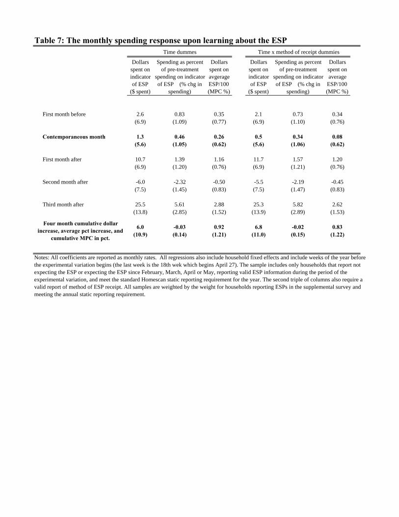
Table 7: The monthly spending response upon learning about the ESPTime dummes Time x method of receipt dummies

Dollars spent on indicator of ESP

($ spent)

Spending as percent of pre-treatment

spending on indicator of ESP (% chg in

spending)

Dollars spent on avgerage ESP/100 (MPC %)

Dollars spent on indicator of ESP

($ spent)

Spending as percent of pre-treatment

spending on indicator of ESP (% chg in

spending)

Dollars spent on average

ESP/100 (MPC %)

First month before 2.6 0.83 0.35 2.1 0.73 0.34(6.9) (1.09) (0.77) (6.9) (1.10) (0.76)

Contemporaneous month 1.3 0.46 0.26 0.5 0.34 0.08(5.6) (1.05) (0.62) (5.6) (1.06) (0.62)

First month after 10.7 1.39 1.16 11.7 1.57 1.20(6.9) (1.20) (0.76) (6.9) (1.21) (0.76)

Second month after -6.0 -2.32 -0.50 -5.5 -2.19 -0.45(7.5) (1.45) (0.83) (7.5) (1.47) (0.83)

Third month after 25.5 5.61 2.88 25.3 5.82 2.62(13.8) (2.85) (1.52) (13.9) (2.89) (1.53)

6.0 -0.03 0.92 6.8 -0.02 0.83(10.9) (0.14) (1.21) (11.0) (0.15) (1.22)

Notes: All coefficients are reported as monthly rates. All regressions also include household fixed effects and include weeks of the year before the experimental variation begins (the last week is the 18th wek which begins April 27). The sample includes only households that report not expecting the ESP or expecting the ESP since February, March, April or May, reporting valid ESP information during the period of the experimental variation, and meet the standard Homescan static reporting requirement for the year. The second triple of columns also require a valid report of method of ESP receipt. All samples are weighted by the weight for households reporting ESPs in the supplemental survey and meeting the annual static reporting requirement.

Four month cumulative dollar increase, average pct increase, and

cumulative MPC in pct.

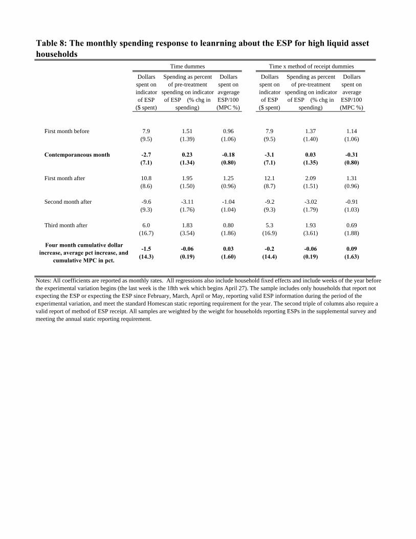
Time dummes Time x method of receipt dummies

Dollars spent on indicator of ESP

($ spent)

Spending as percent of pre-treatment

spending on indicator of ESP (% chg in

spending)

Dollars spent on avgerage ESP/100 (MPC %)

Dollars spent on indicator of ESP

($ spent)

Spending as percent of pre-treatment

spending on indicator of ESP (% chg in

spending)

Dollars spent on average

ESP/100 (MPC %)

First month before 7.9 1.51 0.96 7.9 1.37 1.14(9.5) (1.39) (1.06) (9.5) (1.40) (1.06)

Contemporaneous month -2.7 0.23 -0.18 -3.1 0.03 -0.31(7.1) (1.34) (0.80) (7.1) (1.35) (0.80)

First month after 10.8 1.95 1.25 12.1 2.09 1.31(8.6) (1.50) (0.96) (8.7) (1.51) (0.96)

Second month after -9.6 -3.11 -1.04 -9.2 -3.02 -0.91(9.3) (1.76) (1.04) (9.3) (1.79) (1.03)

Third month after 6.0 1.83 0.80 5.3 1.93 0.69(16.7) (3.54) (1.86) (16.9) (3.61) (1.88)

-1.5 -0.06 0.03 -0.2 -0.06 0.09(14.3) (0.19) (1.60) (14.4) (0.19) (1.63)

Four month cumulative dollar increase, average pct increase, and

cumulative MPC in pct.

Notes: All coefficients are reported as monthly rates. All regressions also include household fixed effects and include weeks of the year before the experimental variation begins (the last week is the 18th wek which begins April 27). The sample includes only households that report not expecting the ESP or expecting the ESP since February, March, April or May, reporting valid ESP information during the period of the experimental variation, and meet the standard Homescan static reporting requirement for the year. The second triple of columns also require a valid report of method of ESP receipt. All samples are weighted by the weight for households reporting ESPs in the supplemental survey and meeting the annual static reporting requirement.

Table 8: The monthly spending response to leanrning about the ESP for high liquid asset households

Table 9: Heterogeneity in weekly spending response by previous income

Time dummes

Income <35,000

35,000< Income <70,000

70,000< Income

Income <35,000

35,000< Income <70,000

70,000< Income

Income <35,000

35,000< Income <70,000

70,000< Income

Week before 0.7 2.4 -0.8 -1.9 -0.4 -0.5 0.12 0.25 -0.08(2.4) (2.7) (3.7) (2.2) (2.0) (2.8) (0.40) (0.27) (0.32)

Contemporaneous week 21.7 15.7 6.3 16.0 10.6 1.9 3.55 1.56 0.53(3.3) (3.2) (3.9) (2.7) (2.4) (2.9) (0.55) (0.33) (0.34)

First week after 17.2 13.0 7.3 13.5 7.4 4.9 2.78 1.29 0.70(2.7) (2.9) (4.1) (2.5) (2.3) (2.8) (0.44) (0.30) (0.36)

65.7 47.2 23.8 6.8 3.6 1.8 10.90 4.68 2.16(10.7) (10.9) (15.9) (1.6) (1.3) (1.6) (1.76) (1.11) (1.41)

Share answering 0.34 0.58 0.08 0.34 0.58 0.08 0.34 0.58 0.08

Time x method of receipt dummies

Income <35,000

35,000< Income <70,000

70,000< Income

Income <35,000

35,000< Income <70,000

70,000< Income

Income <35,000

35,000< Income <70,000

70,000< Income

Week before 1.0 0.6 -2.5 0.5 -2.3 0.5 0.19 0.03 -0.22(2.7) (3.1) (4.1) (2.5) (2.4) (3.1) (0.45) (0.33) (0.37)

Contemporaneous week 20.5 12.8 3.4 18.1 8.0 2.2 3.32 1.26 0.31(3.5) (3.7) (4.3) (3.0) (2.8) (3.2) (0.58) (0.39) (0.38)

First week after 15.9 8.8 1.5 15.3 4.1 3.8 2.69 0.87 0.18(2.9) (3.4) (4.8) (3.2) (2.9) (3.3) (0.49) (0.36) (0.44)

62.9 27.8 -15.7 9.0 0.9 0.7 10.60 2.58 -1.38(14.3) (17.4) (24.8) (2.2) (2.2) (2.4) (2.47) (1.89) (2.28)

Share answering 0.34 0.58 0.08 0.34 0.58 0.08 0.34 0.58 0.08

Notes: See notes for first table of weekly results. ESP averages are taken within groups, so that MPC's represent true differences across groups in propensity to spend from the average ESP for that group.

Dollars spent on average ESP/100 (MPC percent)

Dollars spent on indicator of ESP (dollars spent)

Spending as percent of pretreatment spending on indicator of ESP (percent change in spending)

Dollars spent on average ESP/100 (MPC percent)

Dollars spent on indicator of ESP (dollars spent)

Spending as percent of pretreatment spending on indicator of ESP (percent change in spending)

Seven week cumulative dollar increase, average pct. increase,

and cumulative MPC in pct.

Seven week cumulative dollar increase, average pct. increase,

and cumulative MPC in pct.

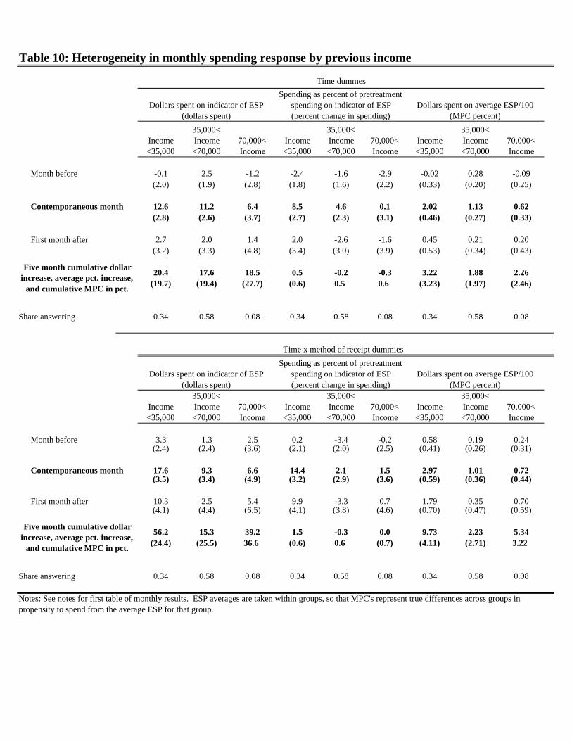
Table 10: Heterogeneity in monthly spending response by previous income

Time dummes

Income <35,000

35,000< Income <70,000

70,000< Income

Income <35,000

35,000< Income <70,000

70,000< Income

Income <35,000

35,000< Income <70,000

70,000< Income

Month before -0.1 2.5 -1.2 -2.4 -1.6 -2.9 -0.02 0.28 -0.09(2.0) (1.9) (2.8) (1.8) (1.6) (2.2) (0.33) (0.20) (0.25)

Contemporaneous month 12.6 11.2 6.4 8.5 4.6 0.1 2.02 1.13 0.62(2.8) (2.6) (3.7) (2.7) (2.3) (3.1) (0.46) (0.27) (0.33)

First month after 2.7 2.0 1.4 2.0 -2.6 -1.6 0.45 0.21 0.20(3.2) (3.3) (4.8) (3.4) (3.0) (3.9) (0.53) (0.34) (0.43)

20.4 17.6 18.5 0.5 -0.2 -0.3 3.22 1.88 2.26(19.7) (19.4) (27.7) (0.6) 0.5 0.6 (3.23) (1.97) (2.46)

Share answering 0.34 0.58 0.08 0.34 0.58 0.08 0.34 0.58 0.08

Time x method of receipt dummies

Income <35,000

35,000< Income <70,000

70,000< Income

Income <35,000

35,000< Income <70,000

70,000< Income

Income <35,000

35,000< Income <70,000

70,000< Income

Month before 3.3 1.3 2.5 0.2 -3.4 -0.2 0.58 0.19 0.24(2.4) (2.4) (3.6) (2.1) (2.0) (2.5) (0.41) (0.26) (0.31)

Contemporaneous month 17.6 9.3 6.6 14.4 2.1 1.5 2.97 1.01 0.72(3.5) (3.4) (4.9) (3.2) (2.9) (3.6) (0.59) (0.36) (0.44)

First month after 10.3 2.5 5.4 9.9 -3.3 0.7 1.79 0.35 0.70(4.1) (4.4) (6.5) (4.1) (3.8) (4.6) (0.70) (0.47) (0.59)

56.2 15.3 39.2 1.5 -0.3 0.0 9.73 2.23 5.34(24.4) (25.5) 36.6 (0.6) 0.6 (0.7) (4.11) (2.71) 3.22

Share answering 0.34 0.58 0.08 0.34 0.58 0.08 0.34 0.58 0.08

Notes: See notes for first table of monthly results. ESP averages are taken within groups, so that MPC's represent true differences across groups in propensity to spend from the average ESP for that group.

Dollars spent on average ESP/100 (MPC percent)

Dollars spent on indicator of ESP (dollars spent)

Spending as percent of pretreatment spending on indicator of ESP (percent change in spending)

Dollars spent on average ESP/100 (MPC percent)

Dollars spent on indicator of ESP (dollars spent)

Spending as percent of pretreatment spending on indicator of ESP (percent change in spending)

Five month cumulative dollar increase, average pct. increase,

and cumulative MPC in pct.

Five month cumulative dollar increase, average pct. increase,

and cumulative MPC in pct.

Table 11: Heterogeneity in weekly spending response by liquid assetsIn case of an unexpected decline in income or increase in expenses, do you have at

least two months of income available in cash, bank accounts, or easily accessible funds?

Time dummes

Answer: Yes No Yes No Yes No

Week before 0.5 1.9 -0.9 -0.8 0.03 0.23(2.1) (2.7) (1.7) (2.2) (0.24) (0.29)

Contemporaneous week 6.6 27.6 3.5 19.2 0.69 3.00(2.4) (3.4) (1.8) (2.8) (0.27) (0.37)

First week after 5.0 24.7 4.0 16.1 0.58 2.66(2.2) (3.1) (1.7) (2.6) (0.25) (0.34)

23.2 83.5 1.7 7.8 2.58 9.06(8.6) (12.1) (1.0) (1.6) (0.97) (1.33)

Share answering 0.60 0.40 0.60 0.40 0.60 0.40

Times x method of receipt dummies

Answer: Yes No Yes No Yes No

Week before -0.3 1.4 0.3 -0.6 -0.10 0.24(2.4) (3.1) (1.9) (2.6) (0.28) (0.35)

Contemporaneous week 5.1 25.5 4.3 18.9 0.53 2.77(2.6) (3.9) (2.0) (3.2) (0.30) (0.43)

First week after 2.9 20.4 4.5 14.3 0.31 2.27(2.6) (3.7) (2.0) (3.4) (0.30) (0.42)

11.7 56.3 2.7 5.6 1.24 6.12(12.5) (18.9) (1.4) (2.6) (1.53) (2.23)

Share answering 0.60 0.40 0.60 0.40 0.60 0.40

Dollars spent on avgerage ESP/100

(MPC %)

Dollars spent on indicator of ESP

($ spent)

Spending as pct of pre-treatment spending on indicator of ESP pct.

chg in spending)

Dollars spent on avgerage ESP/100

(MPC %)

Dollars spent on indicator of ESP

($ spent)

Spending as pct of pre-treatment spending on

indicator of ESP (pct. chg in spending)

Seven week cumulative dollar increase, average pct. increase, and cumulative

MPC in pct.

Notes: See notes for first table of weekly results. ESP averages are taken within groups, so that MPC's represent true differences across groups in propensity to spend from the average ESP for that group.

Seven week cumulative dollar increase, average pct. increase, and cumulative

MPC in pct.

In case of an unexpected decline in income or increase in expenses, do you have at

least two months of income available in cash, bank accounts, or easily accessible funds?

Time dummes

Answer: Yes No Yes No Yes No

Month before -0.3 2.6 -2.9 -0.7 0.00 0.29(1.6) (2.1) (1.3) (1.8) (0.18) (0.23)

Contemporaneous month 5.1 19.4 0.6 11.5 0.58 2.13(2.1) (2.9) (1.8) (2.9) (0.24) (0.32)

First month after 1.8 4.3 -1.6 1.6 0.20 0.54(2.6) (3.7) (2.3) (3.6) (0.29) (0.40)

19.7 28.4 -0.1 0.4 2.22 3.63(15.7) (21.2) 0.4 (0.6) (1.75) (2.32)

Share answering 0.60 0.40 0.60 0.40 0.60 0.40

Times x method of receipt dummies

Answer: Yes No Yes No Yes No

Month before 1.7 3.8 -1.8 0.1 0.27 0.39(1.9) (2.7) (1.5) (2.2) (0.23) (0.30)

Contemporaneous month 6.3 20.5 1.8 14.3 0.82 2.32(2.7) (3.8) (2.1) (3.4) (0.32) (0.44)

First month after 5.3 8.3 0.3 7.1 0.72 1.10(3.4) (4.9) (2.8) (4.4) (0.40) (0.56)

32.9 47.2 -0.1 1.3 4.56 6.67(19.5) (28.8) 0.4 (0.7) (2.27) (3.23)

Share answering 0.60 0.40 0.60 0.40 0.60 0.40

Five month cumulative dollar increase, average pct. increase, and cumulative

MPC in pct.

Notes: See notes for first table of weekly results. ESP averages are taken within groups, so that MPC's represent true differences across groups in propensity to spend from the average ESP for that group.

Five month cumulative dollar increase, average pct. increase, and cumulative

MPC in pct.

Table 12: Heterogeneity in monthly spending response by liquid assets

Dollars spent on avgerage ESP/100

(MPC %)

Dollars spent on indicator of ESP

($ spent)

Spending as pct of pre-treatment spending on indicator of ESP pct.

chg in spending)

Dollars spent on avgerage ESP/100

(MPC %)

Dollars spent on indicator of ESP

($ spent)

Spending as pct of pre-treatment spending on

indicator of ESP (pct. chg in spending)

26

Figure 1: Economic stimulus payments during 2008 as reported by the Treasury and in the raw survey data

Notes: Data from Daily Treasury Statements, April through December 2008 and Nielsen Homescan consumer panel and Economic Stimulus Payment Survey. Homescan statistics are weighted using weights generated for surveyed households with or without static annual reporting requirement for expenditures scaled up by an aggregate factor to account for missing, don't know, and invalid survey data.

0

5

10

15

20

25billions of dollars

Total amounts from Daily TreasuryStatements

Homescan, all surveyed households

Homescan, surveyed households meetingannual reporting requirement

weeks, Sunday to Saturday, dated by starting Sunday