The Education Risk Premium∗†

Kartik Athreya‡and Janice Eberly§

July 2010, revised December 22, 2010

Abstract

College graduates earn substantially higher lifetime income than do workers who do not graduate

college. This skill premium is both persistently high and has increased over time. Nonetheless, the skill

premium has not been accompanied by exceedingly high college enrollment rates: close to one-third of

all high-school graduates currently do not enroll in any form of college.

In this paper, we reconcile observed college enrollment with a high skill premium. We show that when

households face empirically observed failure and earnings risk, even skill premia in excess of current levels

should not be associated, ceteris paribus, with far higher enrollment rates than seen now. We also show

that subsidies to college likely play a very important role in the size of the response of enrollment to skill

premia.

Our findings help explain what Altonji, Baradwaj, and Lange (2008b) term the “anemic” response of

enrollment to changes in the skill premium, and arise from the following simple and intuitive mechanism.

The presence of failure risk generates asymmetric changes in the net return to college investment: those

with low failure risk see a large increase in expected returns, but are inframarginal because they will enroll

under most circumstances. Those with high failure risk see a much smaller increase in expected returns,

and hence remain largely inframarginal. Lastly, despite this dampening effect of risk on enrollment, we

also show that education subsidies of various forms are sufficiently effective to be positive NPV projects

from the point of view of a tax-paying public.

∗Very Preliminary and Incomplete. Do not cite. Do not circulate.†We thank Debbie Lucas and Felipe Schwartzman for useful discussions. We thank Brian Gaines for assistance.‡Federal Reserve Bank of Richmond.§Northwestern University and NBER.

1

1 Introduction

The skill premium is one of the most robust empirical facts in economics. An individual who has completed

college can expect to earn over her lifetime between 1.5 and 1.7 times as much in present value terms as her

non-college-educated counterpart.1 Human capital therefore appears to generate an enormous premium, and

one that far exceeds that historically available on financial market (traded) equity. At its peak, the financial

market equity premium identified by Mehra and Prescott (1985) averaged 6%. By nearly all estimates, the

college premium has consistently averaged approximately twice that much: between 10 and 15%, depending

on the measure used (see, e.g. Goldin and Katz (2000)). A second striking observation concerns the

magnitude of the response of enrollment to changes in the college premium. When measured by the ratio of

hourly wages of skilled to unskilled workers, the college premium increased by nearly 20% between 1980 and

1996 (see Autor, Katz, and Krueger (1998)). However, enrollment did not respond substantially. Over the

period 1979-2005, even though the fraction of young adults (29 years and younger) with a college degree rose

by 9 percentage points (23% to 32%), the increase in male enrollment accounted only for one percentage

point (Bailey and Dynarski (2009)).

The broad trends in college enrollment and the skill premium are shown in Figure 1. At a glance, one

sees that even though enrollment is currently at its historically highest level, approximately one-third of all

high-school completers still do not immediately proceed to any form of college.

Figure 1: Recent Trends in Enrollment Rates and Skill Premia

1See e.g., Restuccia and Urrutia (2004), or Heckman (2007).

1

Averett and Burton (1996) argue further that changes in wage premia by themselves had little effect

on female enrollment rates growing over this period, perhaps reflecting other, more transitional phenomena

arising from broader social changes. Bound, Loevenheim, and Turner (2007) report similar results, showing

not only that enrollment rates failed to rise substantially, but that they even fell for some groups. Moreover,

as documented by these authors, the completion rate for current cohorts has fallen, and those who do

complete appear to take longer to do so. As a result, the overall response of enrollment–and subsequent

skill formation–to changes skill premium itself is typically described as “anemic,” as argued by Altonji,

Bharadwaj, and Lange (2008).

How should one interpret these observations? Should one take the observed premium to college com-

pleters and the apparent insensitivity of enrollment to increases in skill premia as reflective of important

constraints facing households considering investments in human capital? Or, instead, do these features re-

flect compensation for, and responses to, an investment opportunity that is lumpy, irreversible, and most

crucially, risky? The goal of this paper is to address the preceding by posing and answering two more spe-

cific questions. First, what does theory predict that enrollment rates across various ex-ante heterogeneous

groups should be under a given skill premium? Second, given the underlying joint distribution of wealth and

collegiate-preparedness, how large should one expect the response of enrollment of a representative cohort to

be in the face of changes in the college premium?

Our findings are as follows. First, we will demonstrate that a fairly simple model of college enrollment

that is quantitatively accurate in its representation of the lumpiness, irreversibility, and risk inherent in the

college entrance decision can reconcile the high rates on return available to those who succeed with observed

rates of enrollment, as well as the observation that changes in skill premia have not been met with by “large”

changes in enrollment. In particular, we will show that an investment in human capital is unlikely to be a

good deal for significant portions of the US population, even at rates of return that appear, a priori, to be

extremely high, and even when no one is constrained with respect to financing college. Second, we will show

that the underlying heterogeneity in failure risk and wealth is such that a large share of potential college

enrollees are inframarginal with respect to the skill premia. In other words, our benchmark model suggests

that those who did not enroll in college have been, by and large, those who still would not enroll even when

the skill premium increases. Moreover, even to the extent that increases in skill premia increase enrollment

rates, the incremental populations will be increasingly less well-prepared, and will therefore fail at higher

rates than the cohorts who enrolled in the pre-increase period. As a result, the effective increase in the stock

of skilled labor associated with from an increase in the skill premium will be reduced by this composition

effect. Third, our model suggests that current higher education policy, particularly the large direct subsidies

which reduce the out-of-pocket costs for all enrollees irrespective of need or preparedness, are playing an

2

important role. The model shows that as a quantitative matter, when faced with observed skill premia, but

subsidy rates that are much lower than current levels, far fewer would enroll than currently do.

Our emphasis above on the role of uninsurable risks associated with the collegiate investment decision

is motivated by four related pieces of evidence. First, there is abundant evidence for “completion risk,”

measured by the probability that a student will fail to complete college. Failure rates at public 4-year

colleges, which account for the majority of undergraduate enrollment, are approximately 50% (see e.g. Bound,

Loevenheim, and Turner (2007), and NCES (2001)). Second, the uncertainty over eventual completion is

not quickly resolved: it takes, at the median, two years of foregone earnings, and explicit costs of tuition to

realize an earnings stream that may deliver a near zero return. Third, from all available evidence, the return

to partial completion of college is low (i.e. attending but not obtaining a diploma); early documentation

includes Psacharapoulous and Layard (1974), and more recently Hungerford and Solon (1987). Lange and

Topel (2006) argue forcefully that the most reasonable interpretation of this is that students learn about

their future productivity. These authors also take the data as suggesting that the bulk of learning takes

place in the latter parts of college. The lumpiness of initial investment along with the poor returns to non-

completors render failure risk potentially very important to would-be enrollees. Fourth, even upon completing

college, a vast literature, starting perhaps most famously with Lillard and Willis (1978) and continuing to

the present (e.g. Heathcote, Storesletten, and Violante (2009)) has documented the presence of significant

uninsurable idiosyncratic risk (in addition to aggregate risk) in the returns to human capital. Even the

successful college completer is not guaranteed anything. In particular, even college educated households face

earnings processes with substantial persistent (and by several accounts, e.g. Hryshko (2010), nearly unit

root) uninsurable shocks. It is therefore entirely possible for relatively young college graduates to receive

earnings shocks that immediately, and substantially, lower the expected present value of remaining lifetime

income. Finally, the persistence of these shocks also makes them inherently difficult to self-insure as well,

making the absence of market-based insurance more problematic.

One key aspect of our analysis is that we do not impose frictions on credit markets. In part this is because

of the existence of significant policy interventions aimed at ameliorating credit-related impediments to college

financing. In particular, the statutory availability of federally subsidized student loans in amounts capable

of covering the entire cost of most four-year degree-granting institutions (Stafford loans, plus the PLUS

loan program), and the most detailed measurement of borrowing constraints for college-bound households

available to date, that of Carneiro and Heckman (2002), both cast serious doubt on the strength of borrowing

constraints. The latter in particular finds that few households are meaningfully “borrowing constrained” at

the time they decide on collegiate enrollment. Thus, the most commonly cited constraint, that of limits on

the ability of enrollees to borrow, seems unlikely to be a quantitatively important barrier to investment.

3

While the high observed rates of return to investment in human capital cannot easily be ascribed directly

to credit market frictions, credit will in general interact with the frictions we emphasize. Specifically, lever-

age magnifies the impact of uninsurable risks. For a household with currently low wealth and non-trivial

failure risk, for example, financing education with a fundamentally non-contingent instrument, such as debt,

magnifies the risk of failure. Were default possible, this is precisely the type of event in which the bankruptcy

option would be most beneficial to households. It is therefore critical that U.S. government-guaranteed stu-

dent loans are explicitly non-dischargeable in bankruptcy.2 As a result, an enrollee who experiences failure

must lower long-run consumption even more than they otherwise might have to, while also smoothing the

transition. Ex-ante, the lottery over future consumption (especially in the near-term) induced by debt-

financed college enrollment, ceteris paribus, makes college less attractive. We will show that even without

direct credit constraints, students do not always go to college even when the financial returns appear to be

positive.

These results explain why college enrollment is not universal, even when the rate of return appears to

be high, and why enrollment appears insensitive to further increases in the skill premium. Students expect

to receive the skill premium upon college completion. By contrast, education subsidies and financial aid are

conditional only on enrollment, not on completion. Hence, the dampening role of failure risk is reduced,

because students receive the aid regardless of graduation or not. We show that indeed such policies are

somewhat effective in promoting enrollment. Importantly, even accounting for failure risk, we show that

these policies are often positive NPV investment projects from the point of view of the tax-paying public.

The policies counter failure-risk-aversion and encourage a sufficient amount of enrollment and completion

to be self-financing out of subsequent tax revenue. Of course, a fundamental friction in the model is failure

risk itself, so we conclude by examining the benefits of reducing failure probabilities (rather than policies to

counter a given distribution of failure probabilities).

The vast literature on human capital acquisition has long emphasized its importance (see e.g. Altonji

et al. (2008), Goldin and Katz (2008)). Leveling access to education has been viewed as among the least

distortionary ways in which to encourage greater equality within society. To the extent that unequal access to

human capital acquisition is to blame for subsequent inequality in earnings and wealth, expanding educational

opportunities directly limits the growing dispersion in income and wealth that now occurs dramatically over

the life-cycle (see e.g. Storesletten, Telmer, and Yaron (2004)). Of course, education has also long been

viewed as an engine of growth, both through direct effects on the accumulation of a factor of production, but

also through indirect “spillover” effects which hold the promise of increasing returns and thereby efficiency2Recent legislation has allowed for more income-based repayment options to make student loans more equity-like. However,

these options are available only under limited circumstances. In practice, the Department of Education does enforce the

no-bankruptcy rule, making it the largest U.S. garnisher of wages behind the IRS.

4

gains. Our model addresses the first issue, but abstracts from any growth externalities.

Our work is related most closely to early work of Altonji (1993), Chen (2001), and more recently to a

series of quantitative general equilibrium models of higher education. The latter include important papers

of Heckman, Lochner and Taber (1998a,b), and Restuccia and Urrutia (2004). Most recently, related work

includes He (2005), Akyol and Athreya (2005), Garriga and Keightley (2007), Gallipoli, Meghir, and Violante

(2010), Ionescu (2009), Schiopu (2009), and Castex (2009, 2010). Several of the preceding papers study higher

education decisions in settings where enrollees may fail. Aside from our work, fewer papers, however, feature

both failure risk and rate of return risk, with some examples including Chen (2001), Restuccia and Urrutia

(2004) and Akyol and Athreya (2005). A paper that is highly complementary to ours is that of Ionescu and

Chatterjee (2010) who study the problem of how to insure against college failure risk, and in turn, show that

an insurance program can increase enrollment rates substantially—suggesting that risk is indeed a relevant

consideration in enrollment decisions.

The main distinctions between our paper and existing work are twofold. First, while our model structure

shares features in common with existing work, we employ the model rather differently. The previously cited

general equilibrium work first specifies policies, and then aims at understanding their (long-run) implications

for prices (and allocations). By contrast, our approach is to first specify prices–and all other objects that

are parametric to the individual agent–and then analyze the individual-level enrollment decision and ask

what, when aggregated, such decisions should lead one to expect vis-a-vis enrollment and failure.

The approach taken here allows us to address a question of central interest to us: to what extent is a given

skill premium by itself responsible for, or capable of, explaining observed enrollment rates? Relatedly, we ask

to what extent such rates are dependent in important ways on other aspects of the household’s environment,

such as subsidies or need-based aid. Our approach also will help shed light on why certain constellations

of skill premia and policy may not be sustainable as long-run outcomes, as they might be associated with

extremely high or low enrollment rates. A main finding of the model suggests that the current skill premium

is not even close to sufficient for generating observed enrollment. Instead, it is only when current skill premia

are combined with observed rates of subsidies and need-based aid that one generates reasonable enrollment

rates. The insufficiency of the skill premium to spur enrollment is initially surprising, but we will show that

it follows fairly naturally from the presence of risk and heterogeneity in household wealth and preparedness.

Our second innovation is in the modeling structure, which employs the richest model of both failure-

and rate-of-return risk of which we are aware. We are motivated in particular by estimates of Chen (2001)

showing that both transitory and persistent risk components are important in accounting for the rate of

return to college, and our model accommodates both forms of risk.3

3A third, and more minor, distinction between our approach and the preceding literature is that we choose parameters

directly to match their empirically observable counterparts, rather than calibrating parameters such that the model generates

5

2 Model

We study the decision problem of a household in an environment in which college investment carries the three

classes of risk discussed above. First, students must decide whether or not to enroll in college, given failure

risk. Second, subsequent to completion of college investment, and regardless of its success, households will

choose consumption and savings, given earnings risk. Third, all potential enrollees are restricted to the use

of pure non-defaultable debt if their personal resources at the time of enrollment are insufficient to finance

college investment, exposing them to leverage risk.

2.1 Preferences

Households go through three phases in life: they are born Young at which point they make human capital

investment decisions, they work as Adults, and then they are Retirees. Households are Young for K model

periods, to reflect the period between high school and successful college completion. Households then become

workers for J periods, which will be set to reflect the length of time between the age at college completion

and retirement age. Young and Adult households order stochastic processes over consumption using a

standard time-separable CRRA utility function. As Retirees, households value resources taken according to

a “retirement felicity function”, φ, that is defined on wealth xR taken into retirement. All households have

a common discount factor β and discount exponentially.

The general problem for the Young household is to choose consumption ckKk=1 and make risky human

capital investment (enrollment) decisions. Their enrollment decisions will leave them with a human capital

level h ∈ HS,SC,C corresponding either to high school (HS), some college (SC), or college (C) attainment

which, to avoid clutter, we will suppress in the notation below wherever it is obvious. The realized human

capital attainment conditional on the enrolling will depend on the realization of uncertainty over college

completion. When Adults, households then choose consumption cjJj=1, and then wealth xR with which to

enter retirement.

Denote by Θ(Ψ) the set of feasible combinations (ck, cj, xR), given initial state Ψ. The household’s

optimization problem is then:

sup(ck,cj,xR)∈Θ(Ψ)

E0

JXj=1

βjc1−σj

1− σ+ φ(xR) (1)

matching moments. We will show that nonetheless, this parsimonious structure accounts well for the behavior of enrollment

in college and its response to changes in the skill premium. Some details: Ionescu (2009) abstracts from both failure risk and

subsequent riskiness of returns to human capital, which are the risks of central interest in this paper. Ionescu and Chatterjee

(2010), by constrast, allow for failure and moral hazard in effort while enrolled. The model is stylized, and like Ionescu (2009),

abstracts from earnings risk. In addition, for policy analysis, the reader is directed to the particularly rich models of Garriga

and Keigthley (2007) and Gallipoli et al. (2010) who begin, unlike us, by calibrating their model to match enrollment behavior.

6

Retirement felicity as a function of retirement wealth takes the same form as preferences over consumption

in working life, but also includes a weighting factor ν, which will be calibrated.

φ(xR) = νx1−σR

1− σ(2)

This approach is taken in Athreya (2008) and Akyol and Athreya (2010), and offers a convenient way

of generating consumption and wealth accumulation during working life that generates the appropriate

valuations of the college investment given a young agent’s state. It is particularly useful given our focus on

the early-life decision problem of households who face a given skill premium and earnings and failure risk,

as such decisions will remain insensitive to the temporally distant events of retirement.

2.2 Endowments

All agents are endowed with one unit of time, which they supply inelastically.

2.2.1 Labor Income

Young and Adult households face stochastic productivity shocks to their labor supply. Because households

do not value leisure, they are modeled as simply receiving stochastic endowments of the single consumption

good in each period. The income process faced by households in the model is intended to represent precisely

those risks which remain, net of (i) all private insurance mechanisms and (ii) all non-means-tested public

insurance programs, such as the US unemployment insurance system.

A key aspect of our approach is to specify an empirically accurate description of the risk to income,

subsequent to the enrollment decision. The work of Chen (2001) in particular is suggestive in its assessment

of the role played especially by persistent income risk in creating a premium, and thereby being fundamentally

in the nature of a compensating differential, for investment in college. We disaggregate log endowments into

three components: an age-specific mean of log income μj , persistent shocks, zj , and transitory shocks, uj .4

All components of income will depend on the eventual education attainment of an agent, h. Our specification

follows Hubbard et al. (1994), and specifies log income for a household with human capital h to evolves as:

ln yhj = μhj + zhj + u

hj (3)

where

zhj = ρhzj−1 + ηhj , ρh ≤ 1, j ≥ 2 (4)

4Standard specifications of this, are, e.g. Hubbard et al. (1995), Storesletten et al. (2004), Huggett and Ventura (2000).

7

lnuhj ∼ i.i.d N(0,σ2u,h), ln ηhj ∼ i.i.d. N(0,σ2η,h), uhj , ηhj independent (5)

In addition, all household begin life as unskilled households, h = HS, and receive their initial realization

of the persistent shock, z1, from a distribution with different variance than at all other ages. That is,

z1 = ξ (6)

where

ln ξh ∼ N(0,σ2ξ) (7)

The income process can be interpreted as follows. To reflect heterogeneity prior to any direct exposure

to labor market risk, households first draw a realization of the persistent shock z1 from the random variable

ξ with distribution N(0,σ2ξ). In subsequent periods, household non-asset income is determined as the sum

of the the unconditional mean of log income μj , the innovation to the persistent shock ηj and the transitory

shock, uj . The shocks to labor earnings during working age will depend on the human capital level of agents,

to reflect the fact that the risk-characteristics of labor earnings appear to differ systematically by human

capital level (e.g. Chen (2001), Hubbard et. al. (1994, 1995), and Storesletten, Telmer, Yaron (2004)).

2.2.2 Means-Tested Transfer Income

Our model also allows for means-tested transfers, τ(·), represented as a function of current age j, net assets

xj , and income level yj = exp(μj+ zj+ uj). Including this is potentially relevant as it is a source of wealth to

households that may be large enough to alter the decisions of related to college investment. In the benchmark

model, transfers will not depend explicitly on age. Transfers are specified as in the seminal work of Hubbard

et al. (1995):

τ(j, xj , yj) = max0, τ − (max(0, xj) + yj) (8)

and what follows is detailed in Athreya (2008).

2.2.3 Retirement Income

As we stated earlier, households select retirement savings according to the function φ(xR). Following Athreya

(2008), a household’s wealth level at retirement is then the sum of the household’s personal savings xJ+1

and the baseline retirement benefit xτ

xR = xJ+1 + xτ (9)

8

This amount xτ is the wealth level that, when annuitized at the discount rate Rf , and adjusted for the

probability of survival for k periods, πk, yields a flow of income each period equal to the societal minimum

consumption floor τ .5 That is, minimal retirement wealth xτ solves:

KXk=1

πkxτ(Rf )k

= τ (10)

2.3 Young Households and The College Investment Decision

As described above, Young households make decisions for K periods. In the first period, households first

draw income shocks which inform them of their potential income if they decide not to enroll in college. If

they enroll in college, they cannot work. If their private wealth is insufficient to fund college investment,

they must borrow by issuing non-defaultable personal debt. Given the knowledge of both the explicit costs

of college, as well as the level of earnings that will be foregone, households make the decision to enroll or

not in college. If they enroll, they must attend college for τ1 < K periods before they learn whether or not

they will succeed. If they are informed that they will succeed, they have the option to invest the remainder

of their time τ2 ≡ K − τ1 in college, after which they will enter working life as a Skilled agent. Not all

households who are informed of success may choose to continue; they receive earnings shocks in each period,

and a sufficiently high and persistent realization of this random variable may make the expected payoff from

“dropping out” greater than that of continuing. Simultaneously with college investment, Young households

choose consumption and savings. Those choosing to drop out and those failing to succeed then draw income

from the shock process applicable to those with “some college.” Thus, the investment is lumpy, as it does

not offer partial returns for partial investment. Lastly, after τ2 periods, Young households transition to

being Adults, after which they solve a life-cycle consumption savings problem in the face of stochastic,

education-dependent earnings. The preceding structure therefore captures the central features which make

human capital investment risky: leverage, completion risk, lumpiness, irreversibility, and risky returns given

completion.

2.3.1 Recursive Formulation

Given the timing described above, the recursive formulation is straightforward. The state of the household

can be expressed as follows. First, let k and a denote age and household resources at the beginning of the

period. For Young agents the wealth level a should be thought of as the transfer that college-bound children

are expect to receive from their parents. Next, let zτ1 and uτ2 represent the persistent and transitory shocks

to earnings received by households, respectively. Lastly, h and π denote human capital and failure risk,5See again, Athreya (2008) for details.

9

respectively. The state of a household is summarized by the vector x = (k, a, zτ1 , uτ1 , h,π), and to avoid

clutter, in what follows we will refer to the household state by x.

In the first period of being Young, households make the decision to enroll in post-secondary education

by comparing the value of enrollment V E(x) with the value of not enrolling V NE(x). Therefore, we denote

the maximal utility attainable by a young agent in the first period of youth as:

V Y1(x) = max(V E(x), V NE(x))

The value of enrolling is itself the solution to the following problem:

V E(x) = max

∙c1−α − 11− α

+ βτ1¡πEz,uV

F (x0) + (1− π)Ez,uVS(x0)

¢¸subject to the budget constraint if they enroll:

c+ qa0 + τ1Φpvt1 [1− γneed(x)− γmerit(x)− γdirect] ≤ a0

a0 > a

In the preceding, π denotes the probability of failure faced by the enrollee, and V F (·), and V S(·) are the

values of failure and success, respectively, in the first phase of college. The first phase of college takes τ1 units

of time, and therefore future payoffs are discounted accordingly via the term βτ1 . The term Φpvt1 > 0 denotes

the cost of college, prior to all subsidies directly received by educational institutions from state, local, and

Federal sources. Direct subsidies are denoted γdirect, and apply to all enrollees. The terms γneed1 and γmerit1

denote further proportional reductions in the private cost of college arising from need- and merit-based aid,

respectively. Lastly, a0 denotes the wealth or resources available to an enrollee (in general, much of this will

represent parental resources), and in the event that an agent does not enroll, they can earn y(x) as labor

earnings. Insurance markets against income risk are also incomplete, and all agents are endowed with the

ability to save their risk-free assets in a form which earns them return 1/q.

All enrolling students will learn after a period τ1 whether they are performing well enough to successfully

complete college, or must leave. If they remain in college, there is no more uncertainty, and the enrollee

graduates in τ2 units of time. However, since the agent receives a productivity draw in each period, even

those who succeed in the first part of college may choose to drop out. The state vector of a household in the

second phase of Young life is given by: x = (k, a0, zτ1 , uτ1 , h)

These options result in the following value functions. First, the maximal value attainable after a failure

from college, V F (·), satisifies the following recursion:

10

V F (x) = max

∙c1−α

1− α+ βτ2Ez,uV

A(x0)

¸and the flow constraint faced by the household if they fail is:

c+ qa0 ≤ a+ τ2ySC(x)

a0 > a

Next, the value of success in the first phase of college is given by:

V S(x) = max(V C(x), V D(x))

with V C(·) and V D(·) denoting the values of choosing to continue in college, or drop out, respectively. Let

V A(·) denote the value function applicable to Adults. These value functions are given as follows.

V C(x) = max

∙c1−α

1− α+ βτ2Ez,uV

A(x0)

¸subject to the budget constraint that applies to continuing students:

c+ qa0 + τ2Φpvt2 [1− γneed2 (x)− γmerit2 (x)− γdirect] ≤ a

a0 > a

For those choosing to drop out, the value function is:

V D(x) = max

∙c1−α

1− α+ βτ2Ez,uV

A(x0)

¸and the flow constraint they face if they choose to dropout is:

c+ qa0 ≤ a+ τ2ySC(x)

a0 > a

If an agent chooses not to enroll, their decision problem collapses to a standard consumption-savings

problem. In the first period of being Young, they attain a value function that satisfies:

V NE(x) = max

∙c1−α

1− α+ βEz,uV

Y2(x0)

¸

11

where V Y2(·) denotes the maximal value attainable as an agent in the second period of being Young. The

constraint households face in the first period of being Young, if they choose not to enroll is:

c+ qa0 ≤ a+ τ1yHS(x)

a0 > a

In the second period of being Young, given the continuation value V A(·), optimal decisions imply that

V Y2(·) satisfies:

V Y2(x) = max

∙c1−α

1− α+ βEz,uV

A(x0)

¸subject to the associated constraints:

c+ qa0 ≤ a+ τ2yHS(x)

a0 > a

2.4 Adults

Once agents are Adults, they face a finite horizon consumption savings problem, given an income process

which fluctuates about a deterministically evolving mean that reflects the accumulation of experience and

human capital over the life-cycle. Both the shock processes and the evolution of the mean earnings process

will reflect educational attainment. Therefore, optimal decision making of adults will satisfy the Bellman

equation:

V A(x) = max

∙c1−α

1− α+ βEz,uV

A(x0)

¸subject to the flow budget constraint

c+ qa0 ≤ a+ yh(x)

a0 > a

Lastly, in the period immediately prior to retirement, households’ optimal decisions satisfy:

V A(x) = max

∙c1−α

1− α+ βφ(xR)

¸

12

subject to the flow budget constraint

c+ xR ≤ a+ yh(x)

xR > 0

2.5 Aggregating Individual Decisions to Enrollment and Failure Rates

As clarified at the outset, our primary focus will be on understanding the investment decision of a cohort of

young enrollees. To do this, we solve for the flow of new enrollees predicted by theory, under a given expected

skill premium, educational policy, and the joint density of failure risk and available resources for college.

We will show that despite the seeming attractiveness of college from the perspective of risk-neutrality, once

risk-aversion and empirically reasonable measures of failure are taken into account, significant portions of

the population will elect not to enroll in college at current skill-premia.

Given any constellation of behavioral parameters, income process parameters, and educational policy

parameters, household optimization will generate decision rules governing college enrollment. These decision

rules will of course be functions of the household’s state vector. Therefore, the aggregate enrollment flow of

any new cohort of Young agents will depend on the joint distribution describing how Young households are

distributed over the values of these state variables. Letting Γ(x) denote the (cumulative) joint distribution

of Young households over the state vector, and I(·) an indicator function over enrollment in college, the

aggregate enrollment rate, Φ, is given by:

Φ ≡ZI(V E(x) > V NE(x))dΓ

Similarly, the aggregate failure rate is given by:

Π ≡Zf(π|x)dΓ

2.6 Parameters

There are three classes of parameters in the model: those related to preferences, those related to education,

and those related to income and its risks. There are only two preference parameters, the annual discount

factor β, which is set to 0.96, and risk-aversion σ, which is set to 3, as is standard. We turn next to

education-related parameters.

13

2.6.1 Education Related Parameters

To calibrate the investment in education, we choose parameters governing college completion, the cost of

attendance, and student preparedness and resources. We emphasize that we do not set any of the following

parameters to help the model match observables. They are all assigned values based on direct measures

from data. The first parameter is given by the data on the difference in average after-tax lifetime earnings,

which is based on findings of Restuccia and Urrutia (2004) and Chatterjee and Ionescu (2010), is set to 1.5.

The next two parameters are those governing median time-to-failure and time to subsequent completion,

τ1 and τ2, respectively. The next two parameters specify the average subsidy γdirect that is received by

public higher education institutions and the private cost of college Φpvt1 . Turning next to the distribution

of wealth available to potential enrollees, the fifth and sixth parameters specify the mean μa0 and median

mediana0 of the distribution of initial wealth for Youths, which is assumed to be log normal, in line with

SCF data. Similarly, as an empirical matter, the marginal distribution of standardized test scores, e.g. the

SAT, is given by a normal distribution, whose mean and standard deviation we denote by μSAT and σSAT .

This distribution is then translated into a risk of failure that is set to match observed failure rates across

institutions with varying mean SAT scores. We also do not a priori restrict the distributions of standardized

test performance and household resources to be independent. To allow for dependence in a tractable manner,

we assume that these two objects are jointly lognormal, and therefore specify the covariance between test

scores and family resources, which we denote by cov(SAT, a0). The final parameter we choose is the

(common) borrowing limit available to households, denoted by a.

Starting with the parameters governing college completion, the median time to failure is parameterized

according to Fang (2006), as is identical to Akyol and Athreya (2005) (who use NCES data), and is set to

τ1 = 2. Following ([10], Table D-1), college completion time is set at five years, which implies τ2 = 3.6 That

is, college takes five years to complete, and failure, if it occurs, does so at the end of the second year. In the

section on Robustness, we will allow for alternative failure times, and also for a more gradual resolution of

failure uncertainty. The real resource cost of college, Ψpvt1 , is set to match the mean “sticker price” of college.

The upper and lower bounds for this come from adding, or leaving out, room and board. If the former, the

annual cost is approximately $30,393 at 4-year private colleges; if the latter, the cost falls to $21,588.7 The

cost of college to an enrollee is denoted Ψpvt1 = θμcolly where θ is a fraction of mean annual income of college-

educated households. The latter is $75,000 (Census (2007)). Using the midpoint for college costs, we set

θ = 0.35. The level of direct subsidization, prior to any need- or merit-based aid available to those enrolling,

is set to match that prevailing at public four year institutions. It is denoted by γdirectbenchmark, and is measured6The Department of Education compiles a set of studies each estimating the distribution of completion times, and nearly all

of them place the median completion time at 5 years. See http://www2.ed.gov/pubs/CollegeForAll/completion.html7Source: NCES(2008), available at: http://nces.ed.gov/programs/digest/d08/tables/dt08_332.asp

14

by Caucutt and Kumar (2006) at 0.425. Chatterjee and Ionescu (2010) measure the cost of public 4 year

college to be closer to $8000, implying a similar, but slightly higher subsidy rate closer to 0.5. However, some

other measures suggest higher rates of subsidization. In particular, if we measure subsidization rates as the

ratio of the costs of tuition and fees at public four-year colleges relative to that at private four-year colleges,

the rate is 0.72 ($5,950/$21,588, NCES (2008)). The out of pocket cost for tuition and fees in the model is

given by θμcolly γdirectbenchmark. Under our benchmark parameterization, this yields an average cost (tuition plus

fees) of approximately $11,100 annually. To parameterize need-based aid, we follow Clayton and Dynarski

(2007), and employ a simple linear function with two parameters governed by (i) the maximal Pell grant of

$4,000, and (ii) the constant reduction in Pell grants as a linear function of family resources, a0, set such

that it completely disqualifies households with income greater than $50,000.

To set the limit on borrowing by enrollees, as mentioned at the outset, we are guided by the work of

Carneiro and Heckman (2002) who argue that widespread borrowing constraints for education are implausi-

ble. Moreover, there exists at present an explicit set of guaranteed loan programs to finance any amount in

excess of the so-called “Expected Family Contribution.” These are the PLUS loan programs.8 We therefore

will set the debt limit to always allow a household to finance the entire cost of college, given the set of

subsidies that are in place. Specifically, given the costs of college inclusive of all subsidies, we set a, the

borrowing limit that enrolling households face at a = −P2i=1 τ iΨ

pvt1 γdirect.

Since the joint distribution of initial enrollee wealth and enrollee failure risk is specified as bivariate

log-normal, it is governed by five parameters. The first two, which give the distribution of SAT scores is

taken from the College Board, and yields value for the mean and standard deviation of total (critical writing

plus mathematics) SAT scores as μSAT =1000 and σSAT =200, respectively.9 The mean score is also close

(by construction) to the median score.

The available wealth of enrollees will reflect not only their own private resources, if any, but also parental

transfers. The latter, however, are not obviously proxied for by parental wealth, since the willingness of

parents to make such transfers is not directly observable. For the same reason, the level and covariance of

familial resources available to potential enrollees (not just those who ultimately enroll) with test scores is

not well-measured in the data. We use the Survey of Consumer Finances (SCF) from 2004 to compute the

moments of the wealth distribution of households whose head is the median age of the parents of college-

bound students. This yields a lognormal distribution of enrollee initial familial resources with mean μa0=

$40,000 and a median mediana0 = $20,000. Our parameterization specifies that the median transfer to an

enrollee from within the family is on the order of twice median annual household income, and so is not likely8See http://www.fafsa.ed.gov/what010.htm9These numbers are the mean and standard deviation of the total score on the Critical Reading and Mathematics sections

of the SAT. The raw data are here: http://professionals.collegeboard.com/profdownload/sat-percentile-ranks-composite-cr-m-

2010.pdf

15

to understate the actual transfer. As a result, our parameterization is not likely to overstate the benefits

of cost-reductions for college simply by making households counterfactually wealth-poor. This choice is

disciplined by the proportion who receive Pell grants, and the conditional mean of grants among this group.

With respect to the covariance of resources and test scores, it is plausible that while not perfectly positive,

wealth and parental education are strongly correlated and that the latter is in turn correlated with failure

risk (see e.g. Athreya and Akyol (2006) and the references therein). Letting νSAT denote SAT score, we set

cov(νSAT , a0) = 0.3 in our benchmark, which is the midpoint measured of the range estimated by Castex

(2009) for the correlation between “Family Income” and “Ability” (as measured by AFQT) in the NLSY79

and 97. These values are also consistent with students’ self-reported wealth in the demographic section of

the SAT data reported by the College Board. However, because family income and resources available to

enrolling students may not be the same thing, we will examine the effects of alternatives in the Robustness

section. Lastly, to map SAT scored into failure risk, we use observed data on institution-level failure rates

by SAT score to estimate a linear map that takes the percentile of the test scores g(νSAT ) into a probability

of failure as follows: π = 1−λgrad g(νSAT ); where λgrad=0.9.10 We specify g(·) such that the top percentile

of SAT scores will fail with probability (1-λgrad), while the first percentile will fail with probability λgrad.

Table 11 displays the benchmark specification of all education-related parameters in the model.10While in principle there is an issue of selection here, in particular coming from the possibility that those who take the SAT

are disproportionately well-prepared, this is not likely to alter our conclusions, for two reasons. First, there are several states

in the US in which SAT participation rates are very high, and in Maine for instance, it is 100%. The moments of the score

distributions from these states are very similar to that seen amongst only the enrollees at large state universities. Second, if

the bias were to be important, the risk facing most students is actually even greater, making non-enrollment rates even easier

to account for.

16

Main Model Parameters

Parameter Value

Skill Premium 1.5 (Restuccia and Urrutia (2004))

τ1 2 (Fang(2006))

τ2 3 (Bound, Loevenheim, Turner (2007))

θ 0.35 (NCES(2008), Authors’ Calculation)

γdirectbenchmark 0.425 ((Caucutt and Kumar (2005), NCES (2008))

γneed $4,800-0.4a0 (Clayton and Dynarski (2007))

μSAT 1000 (College Board (2010))

σSAT 200 (College Board (2010))

mediana0 $20,000 (SCF 2004)

μa0 $40,000 (SCF 2004)

cov(SAT, a0) 0.3 (Castex (2009))

λgrad 0.9 (Authors’ Calculation from College Board)

a −P2i=1 τ iΨ

pvt1 γdirect

(11)

2.6.2 Income Parameters

Income risk is assigned entirely standard values employed in the literature. We follow Hubbard, Skinner, and

Zeldes (1994), Table A.2, who express age-specific means of after-tax labor income for the three education

groups are given by simple polynomials that are cubic in age. Throughout the paper, we maintain the

assumption that subsidies represent a negligible portion of total government expenditures, and therefore

have negligible tax consequences. The parameters for the stochastic process for shocks to earnings are

described in equations 3 through 7, and summarized below.

Income Risk Parameters

Parameter\Education Level HS Some Coll Coll

σu 0.15 0.15 0.15

ση 0.16 0.16 0.11

σξ 0.5 0.5 0.5

ρ 0.95 0.95 0.95

(12)

3 Results: Enrollment and Risk

First, we provide simple measures of internal rates of return to college. These calculations are sufficient for a

risk-neutral decision maker to choose whether or not to attend college. We then study the implications of our

benchmark model, in which decision makers are risk-averse and prefer intertemporally smooth consumption.

The main focus of our analysis will be to examine the effects of risk on the decision making process of

17

individual agents, and in turn, to show that aggregate implications of our model for college investment,

especially for overall enrollment and failure rates, are very close to the data. This is striking, as no parameters

in the model were set to help match these facts. This gives us confidence that our model indeed captures

the salient forces, especially those related to failure risk. Given this, our final section develops predictions

for the likely consequences of various policies aimed at encouraging collegiate enrollment.

3.1 Risk-Neutrality

We first abstract from risk, and present and compute measures of the “internal rate of return” (IRR). Such

measures will, given the high average skill premium, provide an indication of the “attractiveness” of college.

Indeed, such measures lie behind the intuitive view that college enrollment should be nearly universal and

that failure to enroll is a symptom of resource misallocation.

Internal Rates of Return under US Subsidies

failure risk π = 0.03 π = 0.26 π = 0.50 π = 0.74 π = 0.98

IRR 0.0648 0.0585 0.0486 0.0301 -0.0426(13)

Table 13 reports the discount rate at which a risk-neutral agent with given failure probability π and

direct tuition subsidy rate of 42.5 percent would be just indifferent between enrolling in college or not.

When failure risk is low, say 3 percent, a risk-neutral agent would invest in college for any discount rate

below 6.48 percent. The results indicate that failure risk meaningfully alters the expected benefits from

enrollment. Nonetheless, it is true that for all but the least likely to succeed, a risk-neutral investor would

choose to attend. Even at failure risks of nearly 75%, the internal rate of return exceeds the risk-free rate.

In this sense, the risk-neutral perspective does indeed generate the conclusion that college makes financial

sense for the vast majority of students. If this is so, and if borrowing constraints are so unimportant, why

is the observed enrollment rate fully 30 percentage points short of universal attendance? Our contention is

that the answer lies in the interaction of modest levels of risk-aversion with the lumpy and risky investment

characterizing college, which we now examine.

3.2 Risk-Aversion, Failure-Risk, and the College Investment Decision: TheBenchmark Model

While risk-neutrality is perhaps appropriate as a guide for firms evaluating investment projects, or for

households considering “local” gambles, investment in college is neither conducted by firms, nor is it local

in size. Moreover, as we noted at the outset, many households are not wealthy at the time of the enrollment

decision. These households will have to borrow (being unable to issue equity claims on the fruits of their

18

human capital). Given the size of debts needed for many to finance college, leverage in the relevant amounts

carries a potentially serious risk. For all these reasons, it is a priori likely that risk-aversion plays a significant

role in governing decisions. We therefore turn now to the role played by failure risk by using the model of

enrollment decision-making.

We begin by studying the performance of the benchmark model. This holds fixed all education policies

such as subsidies, need-based, and merit-based aid at currently observed values. We will show that the

model does a good job at describing the decisions of an entering cohort. Specifically, we compare the

model’s performance along two dimensions: enrollment and failure rates.11 Turning first to the unconditional

moments, we see that the model does quite well, as seen next in Tables 14 and 15.

Unconditional Enrollment and Failure Rates

Enroll Rate (Φ) Failure Rate (Π)

Model 0.67 0.45

Data (Bailey/Dynarski (2009)) 0.74 0.43

(14)

Turning next to the more disaggregated relationship between preparedness (as measured by the SAT)

and enrollment rates, we find that the model again does well at generating aggregate enrollment with the

“right” enrollees. The data are taken from Chatterjee and Ionescu (2010).

Enrollment Rates and Test Scores

SAT <900 901-1100 1101− 1250 ≥ 1251Model 33% 86% 97% 97%

Data(Chatterjee/Ionescu (2010)) – 89% 95% 96%

(15)

The key finding from the preceding two tables is that the benchmark model successfully approximates

both aggregate enrollment and failure rates, without being targeted to do so. We now use the model to obtain

predictions for the main question of interest: what should one expect for the enrollment response to a change

in skill premia?

3.3 Failure Risk and The Response of Enrollment to Changes in the Skill Pre-mium

Having described the performance of the benchmark model, and some of its properties, we now turn to one of

the main questions posed at the outset: how should a given cohort’s enrollment behavior change in response

to an increase in the skill premium? The assessment of many (see e.g., Altonji et al. (2008)) is that the11See Bailey and Dynarski (2009), Table 1, for enrollment data, and Table 4 for completion rates. We use the rates reported for

the 1988 birth cohort for enrollment, and the 1982 birth cohort for completion (to allow for suitable length of time to determine

completion). Similar estimates are found in Bound, Loevenheim, and Turner (2007). For example, for completion rates, see

their Table 1 with the 8-year completion rate (proportion of enrollees with bachelor’s degree within 8 years of graduating high

school) among the 1988 NELS cohort being 45.3% and that for the NLS72 group being higher at 51.1%.

19

enrollment response to the steady increase in the skill premium over the 1970s and 1980s has been “anemic.”

Such a view has motivated a variety of policy responses, most notably a substantial increase in Pell Grant

generosity. We use our quantitative model to provide an answer to just how large such a response should

have been expected. Each row gives a value of the skill premium, measured by the ratio of skilled worker

income to unskilled income. Each column gives the enrollment rate in college for a given value of failure

probability. The final column integrates over the distribution of types (in terms of their failure probabilities)

to give the aggregate enrollment rate for a given skill premium.

Enrollment Rates, by Skill Premium and Failure ProbabilityLifetime Prem\π 0.03 0.18 0.34 0.50 0.66 0.82 0.98 Φ

1.4 0.88 0.94 0.93 0.76 0.16 0.00 0.00 0.56

1.5 (benchmark) 1.00 0.97 0.96 0.89 0.33 0.00 0.00 0.67

1.6 1.00 0.98 0.98 0.94 0.47 0.01 0.00 0.74

1.7 1.00 0.99 0.99 0.96 0.56 0.01 0.00 0.77

1.8 1.00 1.00 0.99 0.98 0.70 0.02 0.00 0.82

The final column shows that increases in the skill premium of the magnitude observed, say from 1.5

to 1.7, should not be expected to generate an enormous increase in enrollments; our model predicts that,

ceteris paribus, enrollment should be ten percentage points higher, going from 0.67 to 0.77. As the skill

premium rises further, the response of aggregate enrollment is even smaller: increases in the skill premium

from 1.6 to 1.7 to 1.8, raise enrollments by only three to five percentage points for each increment. These

modest increases in aggregate enrollments mask some dramatic responses for particular groups, however. For

example, taking again the group with failure probability of 66%, the model predicts that enrollment under

the higher skill-premium of 1.7 will be 0.56, compared with the enrollment rate of 0.33 predicted to follow

from a skill-premium of 1.5.

3.4 A Punchline: Most USHouseholds are Inframarginal To College Investment

Taken as a whole, our findings help explain what Altonji, Baradwaj, and Lange (2008b) term the “anemic”

response of enrollment to changes in the skill premium, and arise from the following simple and intuitive

mechanism. The presence of failure risk generates asymmetric changes in the net return to college investment:

those with low failure risk see a large increase in expected returns, but are inframarginal because they will

enroll under most circumstances. Those with high failure risk see a much smaller increase in expected

returns, and hence remain largely inframarginal.

The overall importance of failure risk is seen again in the fact that while a substantial proportion of

households are inframarginal with respect to the return to college, those who are marginal are overwhelmingly

those for whom college investment is genuinely risky–in the sense of carrying a high variance of future utility.

Households who are quite sure to fail or succeed do not face meaningful risk: the variance of future utility

20

induced by an investment in college is low. And as such, the mean return, roughly speaking, will dominate

decision making. In turn, movements in the skill premium are not likely to matter. Specifically, well-prepared

enrollees face low failure risk and so already receive a high rate of return from college under any skill premium

in the approximate vicinity of the current one. Similarly, the ability of the skill premium to meaningfully

alter mean returns for the ill-prepared is minimal. The only remaining question is then: how large is the set

of marginal households? The answer provided by the model is: not very big.

4 Why are So Many Inframarginal? Higher Education Policy and

the Enrollment Decision

We have shown above that incorporating quantitatively reasonable wealth and preparedness heterogeneity

into a model of college investment can account reasonably well for both the level of college enrollment (far less

than universal, even with apparently extremely high returns) and its failure to increase even when the skill

premium rises further. We now ask about the role being played by policy in driving such a large fraction

of each cohort of potential enrollees to be inframarginal with respect to changes in the return to college

investment. Our answer here is that this role is large.

Before addressing the effect of changes in skill premia across different subsidy rates, we first evaluate the

power of direct subsidies to alter decision making under a given skill premium (in this case, the benchmark

lifetime earnings premium of 1.5). Given our primary focus on understanding the decision-making process

leading to college enrollment, we now display enrollment rates and the enrollment decision rule as a function

of both subsidies and preparedness. The Figure 2 documents enrollment rates across subsidy rates and SAT

scores (as a proxy for preparedness levels). This figure shows that under current skill-premia, college is not

financially attractive at low levels of subsidies for even for very well-prepared students, as even top SAT-

scorers enroll at rates below 20% when college is unsubsidized. However, as subsidies rise, the well-prepared

enroll at high rates, while those with middling scores enroll at lower rates. When subsidies reach 50%, in

the broad range of empirically-observed rates for public colleges, students with median scores enroll at very

high rates while less-well-prepared students hardly enroll at all. In essence, Figure 2 shows that the drop-off

of enrollment for less-well-prepared students is very steep, because even subsidized education is not desirable

if the failure probability is too high. The “steepness” of the enrollment surface reflects the fundamental

message of the paper: most are inframarginal. In other words, unless a large mass of household types are

located at a “ridge” where the slope of the surface in any direction is steep (particularly in the direction of

subsidies) one should not expect changes in the underlying environment to yield large changes in enrollment.

21

0

500

1000

1500

0

0.2

0.4

0.6

0.80

0.2

0.4

0.6

0.8

1

SAT Score

Enrollment Rates by SAT score and subsidy rate

Subsidy Rate

Enro

llmen

t Rat

e

Figure 2: Subsidy Policy, Failure Risk, and Enrollment Rates

22

4.1 Wealth and Enrollment: Seeing that Risk Matters

Having described the predictions of our model for the aggregate enrollment behavior of a cohort across

subsidies and failure risk, we turn now to understanding the decisions that underlie the aggregates seen in

Figure 2. In particular, we show “iso-enrollment” contours across three dimension: failure risk, subsidies,

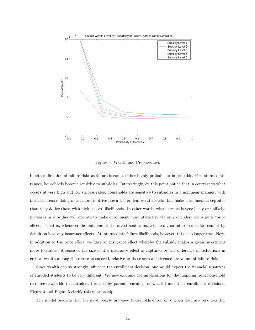
and wealth. Figure 3 is perhaps the most important figure in this paper. It shows the “critical” levels

of personal wealth at which investment in college becomes desirable as a function of the failure risk of an

enrollee, for a variety of subsidy levels. The lowest line is associated with the highest subsidy rate, and the

relationship is monotone. We emphasize three results from this figure.

First, college is not a “no-brainer.” There are many households for whom an unsubsidized investment

in college is simply not financially worthwhile. As can be seen from the figure, if one fixes a wealth level,

then looking across failure risk, we see that for enrollees with a success probability of less than 30%, it takes

a subsidy in excess of 50% before low-wealth households (e.g. those with assets less than $50,000) find it

worthwhile to invest in college.

Second, wealth and preparedness are very clearly substitutes in influencing the decision to enroll. This

is not what would obtain under risk-neutrality: recall that the model does not impose any borrowing con-

straints. Therefore, personal wealth would, under risk neutrality play no role in the investment decision. The

fact that it seems, on the contrary, to play a substantial role in the enrollment decisions of poorly-prepared

households, holding the subsidy fixed, is consistent with risk playing an important role. Moreover, as a

quantitative matter, the relationship is highly nonlinear. Starting in the neighborhood of the unconditional

mean of failure risk in the economy (approximately 54%), we see that under benchmark subsidy rates (the

red line) that an enrollee with no internal wealth would be just indifferent to enrolling or not. But, a less

well-prepared student, with a success probability of 0.25, will only enroll if he has in excess of $10,000 in per-

sonal wealth. As failure probabilities rise, the requisite internal wealth rises rapidly. Subsidies do not change

the qualitative nature of decisions, but alter the threshold level of internal wealth significantly. Under the

lowest subsidy rates, an average would-be enrollee requires approximately $30,000 more internal wealth than

she would under the most generous subsidy regime. This gap persists for even very well-prepared students,

but shrinks for those least-prepared. Intuitively, as the likelihood of failure grows, the subsidy acts as a form

of wealth, as all households wish to enroll, while the subsidy can do little to alter the expected net benefit

for those likely to fail. Moreover, those with a low likelihood of success will face heavy debts from enrolling

unless they have significant internal funds; hence, the vertical distance between critical wealth levels grows

with failure risk. For the highest failure risk however, the subsidy has little influence as the expected return

is deeply negative.

Third, and perhaps most suggestive of the role of risk is that the gap between critical wealth levels shrinks

23

0.1 0.2 0.3 0.4 0.5 0.6 0.7 0.8 0.9 1-5

0

5

10

15

20x 105 Critical Wealth Level by Probability of Failure, Across Direct Subsidies

Probability of Success

Crit

ical

Wea

lth

Subsidy Level 1Subsidy Level 2Subsidy Level 3Subsidy Level 4Subsidy Level 5

Figure 3: Wealth and Preparedness

in either direction of failure risk: as failure becomes either highly probable or improbable. For intermediate

ranges, households become sensitive to subsidies. Interestingly, on this point notice that in contrast to what

occurs at very high and low success rates, households are sensitive to subsidies in a nonlinear manner, with

initial increases doing much more to drive down the critical wealth levels that make enrollment acceptable

than they do for those with high success likelihoods. In other words, when success is very likely or unlikely,

increases in subsidies will operate to make enrollment more attractive via only one channel: a pure “price

effect.” That is, whenever the outcome of the investment is more or less guaranteed, subsidies cannot by

definition have any insurance effects. At intermediate failure likelihoods, however, this is no longer true. Now,

in addition to the price effect, we have an insurance effect whereby the subsidy makes a given investment

more tolerable. A sense of the size of this insurance effect is captured by the difference in reductions in

critical wealth among those sure to succeed, relative to those seen at intermediate values of failure risk.

Since wealth can so strongly influence the enrollment decision, one would expect the financial resources

of enrolled students to be very different. We now examine the implications for the mapping from household

resources available to a student (proxied by parents’ earnings or wealth) and their enrollment decisions.

Figure 4 and Figure 5 clarify this relationship.

The model predicts that the most poorly prepared households enroll only when they are very wealthy.

24

0

500

1000

1500 0

0.2

0.4

0.6

0.8

0

1

2

3

4

x 10 5

Subsidy Rate

The Mean Wealth of Enrollees By Preparedness

SAT Score

Mea

n W

ealth

Figure 4: The Mean Wealth of Enrollees

25

0200

400600

8001000

12001400 0

0.2

0.4

0.6

0.8

0

1

2

3

4

5

x 104

Subsidy Rate

The Mean Wealth of Non-Enrollees by Preparedness

SAT Score

Mea

n W

ealth

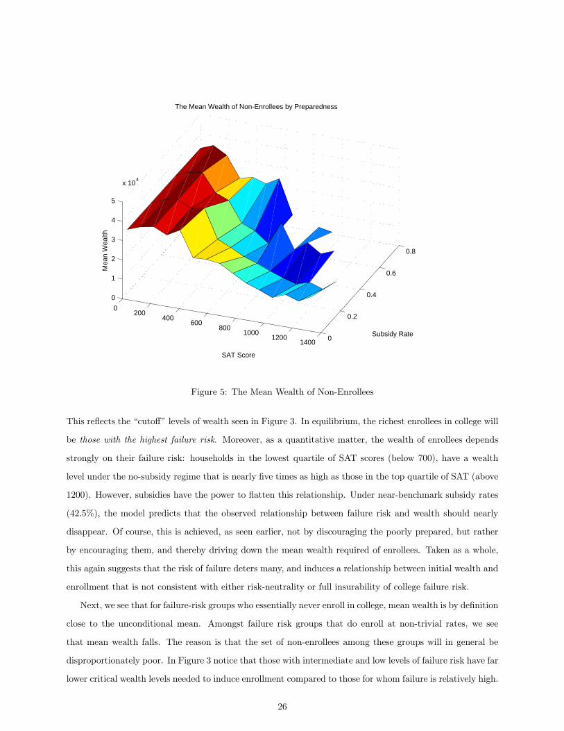
Figure 5: The Mean Wealth of Non-Enrollees

This reflects the “cutoff” levels of wealth seen in Figure 3. In equilibrium, the richest enrollees in college will

be those with the highest failure risk. Moreover, as a quantitative matter, the wealth of enrollees depends

strongly on their failure risk: households in the lowest quartile of SAT scores (below 700), have a wealth

level under the no-subsidy regime that is nearly five times as high as those in the top quartile of SAT (above

1200). However, subsidies have the power to flatten this relationship. Under near-benchmark subsidy rates

(42.5%), the model predicts that the observed relationship between failure risk and wealth should nearly

disappear. Of course, this is achieved, as seen earlier, not by discouraging the poorly prepared, but rather

by encouraging them, and thereby driving down the mean wealth required of enrollees. Taken as a whole,

this again suggests that the risk of failure deters many, and induces a relationship between initial wealth and

enrollment that is not consistent with either risk-neutrality or full insurability of college failure risk.

Next, we see that for failure-risk groups who essentially never enroll in college, mean wealth is by definition

close to the unconditional mean. Amongst failure risk groups that do enroll at non-trivial rates, we see

that mean wealth falls. The reason is that the set of non-enrollees among these groups will in general be

disproportionately poor. In Figure 3 notice that those with intermediate and low levels of failure risk have far

lower critical wealth levels needed to induce enrollment compared to those for whom failure is relatively high.

26

While we do not present it here, at the margin, such households are likely to generate substantial increases

in human capital as subsidies rise, even though their enrollment rates remain low even at high subsidy rates.

We revisit this feature below in the context of the fiscal implications of human capital subsidies. The converse

occurs at high wealth levels, whereby enrollment is consistently high, even at low subsidy rates, while failure

rates are high. For example, under the highest subsidy level, the children of the richest households enroll at

rates exceeding 70%, but those who enroll actually complete at only a 50% rate.

4.2 Enrollment Responses to Changes in Skill Premia: Policy Matters

The results thus far are suggestive of current policy playing a strong role in driving enrollment, and that

successive increases in subsidies will be met with by shrinking, though strictly positive, changes in enrollment

rates. We now turn to the issue of the extent to which enrollment responses to skill premium are altered by

the subsidy policy in place. The results are striking, and are presented below in Table 16:

Enrollment Rate by Subsidy Levels, as the Skill Premium Rises

Skill Premium γdirect = 0.0 γdirect = 0.425 γdirect = 0.75

1.4 0.10 0.57 0.74

1.5 0.18 0.67 0.83

1.6 0.22 0.74 0.86

1.7 0.26 0.77 0.88

1.8 0.30 0.82 0.89

(16)

Two points follow from the results in Table 16. First, skill premia do not appear to be capable of

explaining enrollment by themselves. The unsubsidized cost of college, along with reasonable measures of

the distributions of failure risk and parental resources available to potential enrollees, leaves most households

ambivalent about college–even at high skill premia. Second, when direct subsidies rise from low levels to

higher ones (γdirect = 0 to 0.425) subsidies to higher education matter a great deal for household decisions.

However, at subsidies and skill premia near current levels, additional subsidization (from γdirect = 0.425

to 0.75) does not meaningfully change the response to further increases in the skill premium. This is seen

clearly by comparing the bottom two rows of the Table 16. The message, once again, is that a skill premium

of near 1.5 or greater means that most households are inframarginal with respect to further increases in

expected wages. In other words, both “tails” of the failure risk distribution are inframarginal: those with

high failure risk find that an increase in the skill premium only slightly increases the expected return to

college enrollment.

One way of summarizing the information above is that subsidies matter far more than skill premia

for enrollment. The unsubsidized enrollment rate under the highest skill premium we study (1.8) is far

lower than the enrollment obtaining under the lowest skill premium (1.4) with a 75% subsidy. Relatedly,

27

changes in enrollment only when overall education subsidy policy is very stringent. Under current or higher

subsidization rates, however, changes in skill premia should not be expected to bring forth important changes

in enrollment: the marginal households have been exhausted. One implication of this finding is that if one

views a substantial component of increases in skill-premia arising from shifts in the “demand” for skilled

labor inputs, then it is likely that the net result, barring an increase in subsidization, will be only modest

increases in enrollment. Moreover, given the increasing marginality of the additional enrollee, the resulting

skill formation will likely be even smaller.12 As a result, the model suggests that increases in skill premia

followed by stable enrollment rates may well be a possibilty.

4.3 Subsidies, Grants and Aggregate Enrollment and Failure Rates

Historically, the most important policy aimed at encouraging college enrollment has been the creation of

public college and universities that feature heavily subsidized tuition, and living expenses. In fall 2010, 74%

of college students are enrolled at public colleges and universities (NCES 2010). Having shown above that

subsidies governed the size of the response to skill premia by governing the size of the marginal population,

we now use our model to briefly assess the likely effect of subsidy policies on aggregate enrollment and

completion rates under the benchmark skill premium. Recall that in our model, direct subsidies will not

only reduce the cost of college, but will also reduce the risk faced by students. Subsidies reduce the amount

of wealth devoted, or the amount of borrowing required, to finance college. Given precautionary motives to

avoid low-wealth states, this alters the risk associated with college attendance. Both effects will be larger

for students who are wealth-poor, less-well-prepared, or both.

The enrollment rates as a function of wealth and preparedness, along with the underlying behavior of the

joint distribution of SATs and initial wealth imply the following for aggregate enrollment rates and failure

rates, as a function of subsidies.

Unconditional Enrollment and Failure Rates: Benchmark Skill Premium

Subsidy Rate(γdirect) Enroll Rate (Φ) Failure Rate (Π) Mean Failure Prob (μΠ)

0.0 0.18 0.34 0.54

0.25 0.53 0.42 0.54

0.425 0.67 0.45 0.54

0.5 0.75 0.47 0.54

0.75 0.83 0.48 0.54

(17)

This table integrates enrollment decisions over the underlying joint distribution of SAT scores and initial

wealth available to households of typical enrollment age. As the subsidy rate rises, enrollment responds

strongly. This subsidy is universally available to all students, and (unlike the skill premium) is received12 In the longer run, the net effect of the preceding is likely to lead to greater inequality.

28

regardless of whether or not the student graduates. As more students attend, the selection becomes less

favorable, so the aggregate failure rate rises also. This suggests that while enrollees may be willing to enroll,

that taxpayers as a whole may lose, a question we now turn to.

4.4 Need-Based Aid

The direct subsidies we have studied so far are, by construction, received by all enrollees, and so are a

blunt policy instrument. It is of interest to examine the effectiveness of need-based aid to alter decisions.

Our decision model allows predictions about the long-run effects of changes in such aid. As mentioned in

the Calibration section, we employ a simple representation, based on Dynarski and Clayton (2008) that

provides a good approximation of need-based aid. Specifically, all households face a maximum amount of

need-based aid (what they would get if their familial resources were zero) of $4000. Given this maximum,

the Pell program essentially deducts two-thirds of any additional resources from the maximum amount. As

a result, Pell benefits reach zero at roughly $40000 of household resources. In 2010, the maximal benefit

was increased to approximately $5550, with the reduction for additional resources remaining unchanged. We

therefore look at the effects arising from three levels of maximal Pell grant, $4,100 (‘Pell Level 1’) , $4,800

(‘Pell Level 2’—the benchmark), and $5550 (‘Pell Level 3’). To parallel the earlier discussion, we first show

that the Pell program, which essentially augments household wealth—is likely to have meaningful effects on

the critical wealth levels of households that render them indifferent to enrolling or not. In Figure 6 we see

two things. First, that under current skill premia, for any given subsidy rate, the higher the Pell grant, the

lower the critical wealth level that makes college worthwhile. Second, the higher the subsidy rate, the less

that the Pell grant matters, as is natural.

The overall impact of the Pell program depends not just on the wealth thresholds described above, but

also on the characteristics of the joint distribution of wealth and standardized test scores. The following

Table shows the results for these values of the Pell program for all the agent types in the economy. Given

the positive correlation between wealth and collegiate preparedness, the recipients of need-based aid will

disproportionately be drawn from a relatively less well-prepared population. The following Table shows the

model’s predictions for the response of enrollment by failure-risk type to systematic increases in the generosity

of the Pell Grant program. Each row of the table gives the enrollment rate for a given maximum Pell grant,

varying across failure probabilities in each column. The final column integrates over the distribution of

failure probabilities to give the aggregate enrollment rate.

Enrollment rate by Failure Risk and Pell Grant Maximum

29

0 0.1 0.2 0.3 0.4 0.5 0.6 0.7 0.8-1

-0.5

0

0.5

1

1.5x 105 Critical Wealth Level by Subsidy 1 Level, Across Pell Levels

Subsidy 1 Level

Crit

ical

Wea

lth

Pell Level 1Pell Level 2Pell Level 3

Figure 6: Subsidies and Pell Grants

Pell Max \π 0.03 0.18 0.34 0.50 0.66 0.82 0.98 Φ

$4,100 1.00 0.97 0.94 0.86 0.25 0.00 0.00 0.65

$4,800 (benchmark) 1.00 0.97 0.96 0.89 0.33 0.00 0.00 0.67

$5,550 1.00 0.97 0.98 0.90 0.40 0.00 0.00 0.71

The results in the final column suggest that under the benchmark parameterization, modest increases in

need-based aid of the magnitude we have observed can be expected to generate modest increases in enroll-

ment. The issue here is that the increase in need-based aid is small compared to the subsidy already available

(57% in the benchmark). Once again, these results highlight the inframarginality to college investment of

most households. Students with low wealth and a good chance of success are already enrolled (see the first

four columns above), while those with weak preparedness tend not to enroll (see the last two columns with

π = 0.82 and higher). A small grant does not, for most potential enrollees, overcome the cost of school which

must be paid even if graduation is not attained. Nonetheless, we see that a substantial change for enrollees

with a failure risk of π = 0.66.

30

5 The Fiscal Implications of College Financial-Aid: Are College

Subsidies a Good Investment for Taxpayers?

In this section, we evaluate the value of subsidies from a more narrow fiscal perspective by measuring the

return the government (and hence, taxpayers) receive for investments in the human capital of young cohorts

that arise from our model of enrollment decisions. We will hold the skill premium fixed throughout, something

that allows for comparability across subsidy rates, but also provides a good approximation given that the

flow of new enrollees, in whom we are interested, will constitute only a small proportion of the overall stock

of college-educated workers.

Specifically, we calculate the net present value (in per student terms) arising from the initial investment

in educational subsidies, followed by increased income tax receipts for the remainder of working life, collected

from those who succeed. At low levels of subsidies, the NPV of college subsidies may increase as subsidies

rise. This is because, as we showed earlier (see, e.g. Figure 3), low wealth can present a serious barrier to even

well-prepared students without borrowing constraints. As a result, if potential enrollees respond strongly to

subsidies, the net payoff to taxpayers can be positive: many marginal enrollees will be well-prepared, will

therefore succeed frequently at college, and given the high skill premium and non-trivial average tax rate

that applies, will repay the taxpayers in excess of the initial investment. Of course, not all will succeed,

and in fact, as subsidies get larger, enrollees will, as seen earlier, be progressively less well-prepared. As

a result, even abstracting from the potential for lower ex-post returns to college among those with higher

ex-ante failure probabilities, a government will eventually be financing more poorly prepared students. Still,

the NPV may still remain positive even at very high subsidy rates, something which crucially depends on

the size of the skill premium. Eventually the marginal payoff from increasing the subsidy or need-based aid

is likely to begin to decline.

The specific calculations we make are the following. For a given value of need-based aid, γneed, and given

a subsidy rate γdirect, the population (measure) of young agents μYπ of failure-type π, and the full annual

unsubsidized cost of college, Φpvt1 , we first solve the model to obtain enrollment rates Φπ for each failure-risk

group. Given this, we then calculate the total present value of public investment in a college-bound student

as follows:

Ipublic(γdirect,π|γneed) = μYπ Φπ[γdirectΨpvt1 τ1 + (1− π)γdirectΨpvt2 τ2]

That is, the total cost to the fiscal authority is the per-enrollee expenditure in the first part of college,

γdirectΨpvt1 τ1, and if the student is successful, which occurs with probability π, again in the second part of

college, γdirectΨpvt2 τ2 times the total number (measure) of enrollees of failure-risk-type π, μYπ Φπ.

The revenue generated by this public-sector investment is the flow of additional tax revenues received by

31

the fiscal authority in taxes implied by the skill-premium multiplied by the tax rate. Denote by ωC_pre−taxj

and ωjHS_pre_tax the pre-tax age-specific mean levels of earnings for college- and high-school-educated

households, respectively. Assuming that the taxes T ∈ [0, 1] are levied as flat proportions on labor earnings

alone, and given a public-sector discount factor Q, we have the present value of flows arising from a subsidy

level γ to a failure-risk-type π as Ωpublic:

Ωpublic(γ,π) =JXj=1

Qj(ωC_pre−taxj − ωj

HS_pre_tax)μYπ Φπ(1− π)T

The net present value to the public of a subsidy program of generosity γ targeted at failure-risk-group π

is then simply:

NPV (γ,π) = −Ipublic(γdirect,π|γneed) +Ωpublic(γ,π)

As stated earlier, we assume that the incremental increase to taxes arising from an expansion of the

subsidy program are negligible. Therefore, we present calculations under the presumption of an overall flat

tax rate T of 25% that remains constant across subsidy levels. We set Q = 0.96 to reflect a 4% discount rate

by the government.13

5.1 Direct Subsidies and Merit Aid

Since the most common way to reduce the cost of college is to provide subsidized tuition, we first examine

the net present value implications of providing subsidies, and collect the results in the Table 18. Each row

of the table gives the NPV as calculated above for a given subsidy rate. Each column gives the NPV for a

given failure probability cohort. By looking at a column alone, we can also measure the NPV of giving aid

to a particular preparedness cohort, which is a version of merit-based aid. In other words, fix a class of agent

in terms of failure risk, and fix a subsidy regime. Then ask: “given that the set of agents with such failure

j risk, facing such a subsidy i, currently enroll at rate Φij , what is the net present value to the government

of giving this class of youth this subsidy?”14 Of course, the issue for the government-as-investor is whether

the incremental enrollees (those enrolling in response to the change in subsidy) subsequently earn enough to

offset the public’s investment in their education. This is because under any given subsidy regime, many will

be inframarginal. Therefore, we will present the changes in NPV (γ,π) arising from systematic increases in

subsidy levels. The results are given below.13This is equivalent to the discount rate of the agent for simplicity, and also to reflect the notion that much of the failure

risk faced by agents is diversifiable from the point of view of the government. This should not suggest, however, that the

government’s investment is risk-free. The stream of tax revenue has systematic risk, which the government bears and should

be priced. We include higher discount rates in our robustness calculations to allow for this risk.14Of course, under a subsidy rate of zero, the net present value is positive, and simply represents the present value of tax

collections from a given cohort (of a given failure-risk type) over their lifetime. Once the subsidy is strictly positive, these

benefits get partially offset by the costs of providing the subsidy.

32

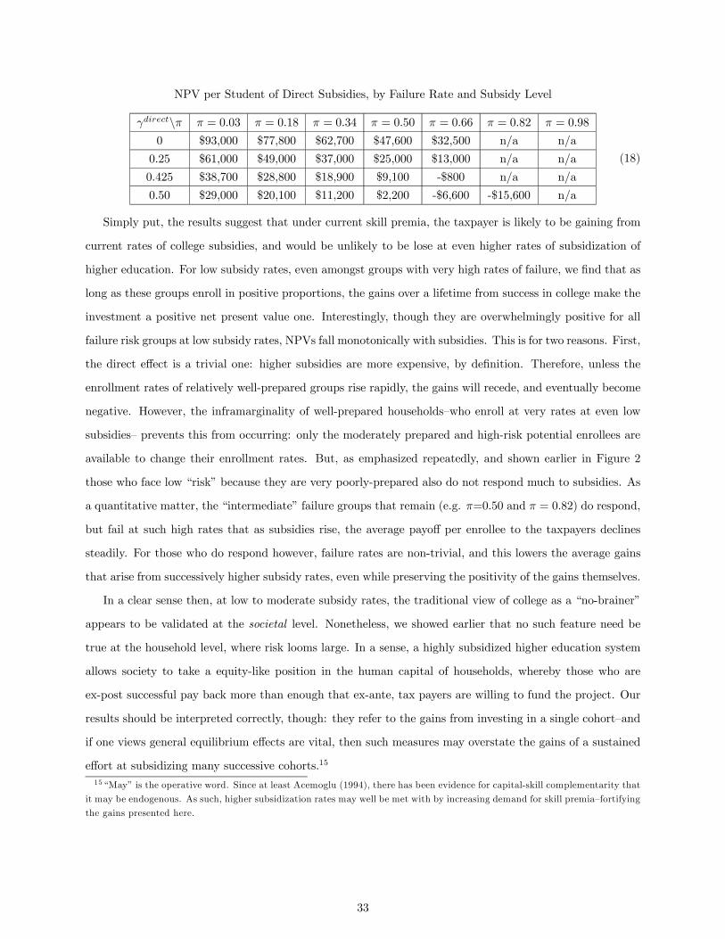
NPV per Student of Direct Subsidies, by Failure Rate and Subsidy Level

γdirect\π π = 0.03 π = 0.18 π = 0.34 π = 0.50 π = 0.66 π = 0.82 π = 0.98

0 $93,000 $77,800 $62,700 $47,600 $32,500 n/a n/a

0.25 $61,000 $49,000 $37,000 $25,000 $13,000 n/a n/a

0.425 $38,700 $28,800 $18,900 $9,100 -$800 n/a n/a

0.50 $29,000 $20,100 $11,200 $2,200 -$6,600 -$15,600 n/a

(18)

Simply put, the results suggest that under current skill premia, the taxpayer is likely to be gaining from

current rates of college subsidies, and would be unlikely to be lose at even higher rates of subsidization of

higher education. For low subsidy rates, even amongst groups with very high rates of failure, we find that as

long as these groups enroll in positive proportions, the gains over a lifetime from success in college make the

investment a positive net present value one. Interestingly, though they are overwhelmingly positive for all

failure risk groups at low subsidy rates, NPVs fall monotonically with subsidies. This is for two reasons. First,

the direct effect is a trivial one: higher subsidies are more expensive, by definition. Therefore, unless the

enrollment rates of relatively well-prepared groups rise rapidly, the gains will recede, and eventually become

negative. However, the inframarginality of well-prepared households—who enroll at very rates at even low

subsidies— prevents this from occurring: only the moderately prepared and high-risk potential enrollees are

available to change their enrollment rates. But, as emphasized repeatedly, and shown earlier in Figure 2

those who face low “risk” because they are very poorly-prepared also do not respond much to subsidies. As

a quantitative matter, the “intermediate” failure groups that remain (e.g. π=0.50 and π = 0.82) do respond,

but fail at such high rates that as subsidies rise, the average payoff per enrollee to the taxpayers declines

steadily. For those who do respond however, failure rates are non-trivial, and this lowers the average gains

that arise from successively higher subsidy rates, even while preserving the positivity of the gains themselves.

In a clear sense then, at low to moderate subsidy rates, the traditional view of college as a “no-brainer”

appears to be validated at the societal level. Nonetheless, we showed earlier that no such feature need be

true at the household level, where risk looms large. In a sense, a highly subsidized higher education system

allows society to take a equity-like position in the human capital of households, whereby those who are

ex-post successful pay back more than enough that ex-ante, tax payers are willing to fund the project. Our

results should be interpreted correctly, though: they refer to the gains from investing in a single cohort—and

if one views general equilibrium effects are vital, then such measures may overstate the gains of a sustained

effort at subsidizing many successive cohorts.15

15 “May” is the operative word. Since at least Acemoglu (1994), there has been evidence for capital-skill complementarity that

it may be endogenous. As such, higher subsidization rates may well be met with by increasing demand for skill premia—fortifying

the gains presented here.

33

5.2 Universal Tuition Subsidies

The preceding results are important to policy decisions in cases where the subsidy can be targeted by failure

risk. In essence, limiting subsidies to particular subgroups on the basis of the NPV calculations would

function as merit-based aid. Now, we consider the case in which the government has no such ability, and

instead must offer a subsidy rate that is accessible to all enrollees. Naturally, this will shrink the overall NPV

of such a change, as the enrollment responses of the poorly-prepared will factor in along with the increased

enrollment, at least at low subsidy levels, of the well-prepared. Specifically, the calculation we present is

as follows. Let P (π|enroll) denote the probability of a household being of failure-type k, given that it has

enrolled. This is an input that allows then to compute the overall measure (size) of each failure group in

the pool of enrollees. Given this, the unconditional expected NPV, E(NPV ), to government just takes the

NPVs for each failure risk group (holding fixed the subsidy), and then weights each group by the preceding

probability distribution. That is, we define E(NPV ) =P

πNPV (γ,π)P (π|enroll). We now assess the payoff

to the public’s investment in a universal subsidization scheme for higher education. The results are reported

in following Table.

Direct Subsidies and Unconditional NPV, by Failure Rate

γdirect E(NPV ) Φ Π

0.00 $44,400 0.18 0.34

0.25 $23,500 0.53 0.42

0.425 $8,800 0.68 0.45

0.50 $1,300 0.75 0.46

(19)

The main finding here is that this reflects, in yet another way, the importance of the size of the infra-

marginal population. Namely, as the subsidy goes up, this number stays essentially flat, mainly because the

well-prepared students enroll at extremely high rates, and the higher the subsidy, the more badly-prepared

enrollees there are (as seen by the failure rates in the third column). Nonetheless, current subsidy rates

appear to be substantially positive NPV.

However, on balance, the most noticeable feature is the fact that an unrestricted subsidy program pro-

duces substantial gains, even at high subsidy rates, and even when the aggregate failure rate is high. The

results are driven by the fact that the high skill premium, even when college success is remote ex-ante, trump

the costs of failure—especially when these costs are automatically truncated by the fact that failure occurs

relatively early in the college experience. Hence, subsidies encourage more experimentation, and even when

few succeed, the payoff to success is high.

34

6 How much are programs that alter failure risks likely to be

worth?

The results presented thus far have all been aimed at understanding the role played by failure risk in a setting

in which the underlying distribution of preparation has been taken as given. However, the efficacy of the

policy changes we have considered have all depended importantly on their interaction with the distribution

of college success. Given the centrality of failure risk, it may be most important to instead better understand

the extent to which altering the distribution of collegiate-preparedness may in fact be the relevant policy

instrument. Such programs might involve more rigorous high-school curricula, as well as more active inter-

vention into the pre-collegiate experiences of potential entrants. Our model allows features three sources

of risk: initial wealth, the randomly determined ability to complete college, and the waiting time for the

uncertainty over collegiate success to resolve itself. We will focus on understanding the extent to which the

latter two would be worth pursuing.

Specifically, we conduct two classes of experiments. First, we consider the gains available from putting

in place measures that will detect an inability to complete college at an earlier date. That is, we consider

the effect on enrollment and NPVs from reductions in τ1, the date at which students learn weather they will

succeed or fail in college. We then allow for changes in the overall preparedness of high-school completers.

Specifically, we study allocations obtained from a setting in which a given SAT score is associated with a

κ−percent reduction in the likelihood of failure. Here again, we will ask the extent to which there are gains

available, and compare them to the gains from increased subsidies.

[TO BE COMPLETED]

6.1 Implications of Fiscal Federalism

We noted earlier that one of the most important college subsidy programs is the existence of modestly priced

state colleges and universities. The fiscal implications of this subsidy require a different parameterization of

our fiscal model, since most states have lower tax rates than the 25% we use above. These states ultimately

recoup their investment under the presumption that those who are subsidized remain in state an pay taxes.

To examine this hypothesis, we consider outcomes from a variety of settings for the two parameters that

govern the NPV reaped (or paid) by a given state. These are, respectively, the state’s share of subsidies ψs,

and the state’s tax rate relative to overall tax rates, τs. The results are given for the NPV arising from a

regime in which the benchmark subsidy of 42.5% is in place.

[TO BE COMPLETED]

35

7 Conclusions

We have shown that a high and increasing college skill premium can be reconciled with the observed level and

response of college enrollment, which has been termed “anemic” by higher education researchers. Empirically

reasonable measures of college failure risk and income uncertainty deter enrollment when potential students

are uninsured and especially when they are also leveraged. The model replicates both the observed enrollment

rate of college graduates, their subsequent failure experience once in college, and the manner in which the

enrollment rates responds to increases in the skill premium.

Our findings, especially those that examine household decision-making, emphasize that while the return

to higher education is high, it is not a safe investment for many households. The deterrent effect of risk

survives the ability of agents to feasibly debt finance college with student loans. The main force here is that

debt makes higher education riskier for student borrowers, suggesting that alternatives that are mindful of

risk may be more effective. In turn, the focus of the policy experiments we consider is on direct subsidies

and need-based aid, both of which help lower the risk over future utility induced by college.

Ideally, as was noted many years ago by Milton Friedman, equity financing is one way to reduce failure

risk, because the equity “investor” shares some of the risk with the student. While we have not explicitly

modeled equity-financing of higher education, its risk-sharing properties are implicit in both the direct

subsidy programs and need-based grant aid we consider. In particular, this is effectively what the government

does when it subsidizes education and then recoups its investment through income taxation that is either

neutral (flat-rate) or progressive. Under a flat-rate tax system of empirically reasonable magnitudes, we have

shown that these investments tend to be positive NPV to the government: the present value of a share of

the skill premium exceeds the cost of the subsidy provided.

While our results emphasize the impact of failure risk, as a given, on the enrollment decision, we are

currently examining the effect of reducing failure risk, by increasing student preparedness directly. We expect

that the impact of improving student preparedness would be large in our model.

Two further caveats are in order. First, we have assumed that the skill premium, and indeed all of the

parameters in the model, are fixed and known to potential students in advance. Uncertainty about the skill

premium, and in particular the possibility that it may decline, may further deter enrollment. The financial

aid policy parameters are also fixed. However, subsidy parameters are only relevant for the period while in

college, and so this imposes a weaker assumption than the lifetime skill premium we have assumed. However,

we do assume that loans continue to be non-dischargeable and that other long run features of student lending

do not change.

Second, we have also abstracted from substantial and interesting heterogeneity among schools. We have

parameterized the enrollment decision to a public four-year institution. Public higher education enrolls the

36

majority of college students (74% of all college students), so we view this parameterization as capturing

the cost structure facing the marginal student deciding whether or not to enroll in college. Those who

enroll in more expensive schools face higher costs, so we assume that they would surely have enrolled in the

”cheaper” school that we model and hence this variation does not change our calculations of the enrollment

rate. Nonetheless, the structure we employ could be used to model the distribution of students across schools,

where the returns to attending various schools could vary along with their costs. This would be an interesting

extension and application of the framework we develop here.

37

References

[1] [To be completed!]

[2] Abel, Andrew, and Janice Eberly, “Q Theory Without Adjustment Costs & Cash Flow Effects Without

Financing Constraints,” working paper, 2001.

[3] Akyol, A., and K.Athreya, 2005, “Risky Higher Education and Subsidies,” Journal of Economic Dy-

namics and Control, 29(6), 979-1023.

[4] Altonji, J., 1993. The Demand for and Return to Education When Education Outcomes are Uncertain.

Journal of Labor Economics 11, 48-83.

[5] Altonji, Joseph G., Prashant Bharadwaj, and Fabian Lange (2008), “Changes in the Characteristics of

American Youth: Implications for Adult Outcomes”, NBER Working Paper 13883.

[6] Altonji, Joseph G., Prashant Bharadwaj, and Fabian Lange (2008b), The anemic response of skill

investment to skill premium growth, www.voxeu.org., acceessed 8/10/09/

[7] Autor, David, L. Katz, and A. Krueger, 1998, “Computing Inequality: Have Computers Changed the

Labor Market?,” Quarterly Journal of Economics, 113(4), 1169-1213.

[8] Averett, S, and M.Burton, 1996, “College Attendance and the College Wage Premium: Differences by

Gender”, Economics of Education Review, 15(1), 37-49.

[9] Bailey, M, and S. Dynarski, 2009, “Inequality in Postsecondary Attainment: An Historical Perspective”,

Working Paper, Brookings Institution

[10] Bound, J., M. Loevenheim, and S. Turner, 2007, “Understanding the Decrease in College Completion

Rates and Increased Time to the Baccalaureate Degree,” Population Studies Center Research Report

07-626.

[11] Castex, G., 2009, “Accounting for the College Attendance Profile,” mimeo, University of Rochester

[12] Castex, G., 2010, “College Risk and Return”, mimeo, University of Rochester

[13] Carneiro, P., and J.Heckman, 2002, “The Evidence on Credit Constraints in Post-Secondary Schooling,

112, 705-734.

[14] Caucutt, E., and Kumar, K., 2003. Higher Education Subsidies and Heterogeneity: A Dynamic Analysis.

Journal of Economic Dynamics and Control 27, 1459-1502.

38

[15] Chen, S., 2001. Is Investing in College Education Risky? University of Rochester and SUNY Albany.

Mimeo.

[16] Clayton, J, and Dynarski, S. 2007, “College Grants on a Postcard: A Proposal for Simple and Predictable

Student Aid” (with Susan M. Dynarski). Hamilton Project Discussion Paper 2007-01. Washington, DC:

The Brookings Institution.

[17] Fang, H., 2006, “Disentangling The College Wage Premium: Estimating a Model with Endogenous

Education Choices”, International Economic Review, 47(4), 1151-1185.

[18] Gallipoli, G., Meghir, C., and Violante, G, 2010, “Education Decisions and Policy Interventions: A

General Equilibrium Evaluation” NYU Working Paper

[19] Goldin, C., and L. Katz, 2008, The Race Between Education and Technology, Harvard University Press,

Cambridge, MA.

[20] Heckman, J., Lochner, L., and Taber, C. 1998a, “Explaining Rising Wage Inequality: A Dynamic Gen-

eral Equilibrium Model of Labor Earnings with Heterogeneous Agents,” Review of Economic Dynamics,

1: 1, 1-58.

[21] Heckman, J., Lochner, L., and Taber, C. 1998b, “General Equilibrium Treatment Effects: A Study of

Tuition Policy”, American Economic Review P&P 88:2

[22] Heathcote, J., Storesletten, K., Violante, G., 2005. “Two Views of Inequality Over the Life Cycle,”

Journal of the European Economic Association 3, 765-775.

[23] He, H., 2009, “What Drives the Skill Premium: Technological Change or Demographic Variation?”,

Working Paper, University of Hawaii at Manoa, 2009-11.

[24] Hubbard, G., Skinnner, J., Zeldes, S., 1994, “The Importance of Precautionary Motives in Explaining

Individual and Aggregate Saving,” Carnegie-Rochester Conference Series on Public Policy, 40(1), 59-125.

[25] Hubbard, G., Skinnner, J., Zeldes, S., 1995. “Precautionary Saving and Social Insurance.” Journal of

Political Economy 103, 360-99.

[26] Huggett, M., Ventura, G., 2000. Understanding Why High Income Households Save More Than Low

Income Households. Journal of Monetary Economics 45, 361-397.

[27] Hryshko, D., 2010, “RIP to HIP: The Data Reject Heterogeneous Labor Income Profiles” mimeo,

University of Alberta.

39

[28] Hungerford, T., and G.Solon, 1987, “Sheepskin Effects in the Returns to Education”, The Review of

Economics and Statistics, 69(1), 175-77.

[29] Ionescu, F., 2009, “Risky College Investment under Alternative Bankruptcy Regimes for Student Loans”

Working paper, 2009-01, Colgate University.

[30] Ionescu, F., and S. Chatterjee, 2010, “Insuring College Failure Risk,” Working Papers, 10-1, Federal

Reserve Bank of Philadelphia.

[31] Lange, F., and R. Topel, 2006, “The Social Value of Education and Human Capital”, Handbook of

Education Economics, 1.

[32] Layard, R., and G. Psacharapoulos, 1974, “The Screening Hypothesis and the Returns to Education”,

Journal of Political Economy, 82(5), 985-98.

[33] Lillard, L., and Willis, R.J., 1978, “Dynamic Aspects of Earning Mobility”, Econometrica, 46(5), 985-

1012.

[34] Mehra, R, and Prescott, E. 1985 The Equity Premium: A Puzzle, Journal of Monetary Economics

[35] Restuccia, D., and Urrutia, C., 2004. Intergenerational Persistence of Earnings: The Role of Early and

College Education. American Economic Review.

[36] Storesletten, K., Telmer C., Yaron A., 2004. Consumption and Risk-Sharing over the Life Cycle. Journal

of Monetary Economics 51, 609-33.

40

8 Appendix: Robustness [to be completed]

8.1 Sensitivity to Risk and The Roles of Risk-Aversion and Discounting

8.1.1 Risk-Aversion

8.1.2 Discounting

8.2 The Importance of Household Wealth on the Fiscal Consequences of PublicSupport for College

All of these effects are enhanced in settings where the wealth of enrolling households is relatively lower, and

stunted in the opposite case.

8.3 The Interaction of Failure Risk and Low Familial Resources

In this section we demonstrate that initial wealth has important effects on enrollment decisions. We study

enrollment in the case where the distribution of parental resources available to enrollees at the time of

enrollment is halved from that used in the benchmark. Specifically, median parental transfers are lowered

to $5000, while the mean is set to $10,000. The most prominent form way to deal with the presence of

households with low availability of resources has been to ensure that guaranteed loan programs exist to

finance college, and the need-based aid for college is that provided by the Federal Pell Grant program. We

first assess the likely impact of direct subsidies..

41