The Effects of Upcoding, Cream Skimming

and Readmissions on the Italian Hospitals

Efficiency: a Population–based Investigation

Paolo Berta†, Giuditta Callea§∗, Gianmaria Martini§ and Giorgio Vittadini†

June 2009†CRISP, University of Milan Bicocca, Department of Quantitative Methods, Italy, §University of

Bergamo, Department of Economics and Technology Management, Italy

AbstractIn this paper we analyze the effects of some distortions induced byprospective payment system, i.e. Upcoding, Cream Skimming andReadmissions, on hospitals’ technical efficiency. We estimate a pro-duction function using a population–based dataset composed by allactive hospitals in an Italian region during the period 1998–2007. Weshow that cream skimming and upcoding have a negative impact onhospitals’ technical efficiency, while readmissions have a positive ef-fect. Moreover, we find that private hospitals are more engaged incream skimming than public and not–for–profit ones, while we observeno ownership differences regarding upcoding. Not–for–profit hospitalshave the highest readmission index. Last, not–for–profit and publichospitals have the same efficiency levels, while private hospitals havethe lowest technical efficiency.

JEL classification: C51, I11, I18, L33Keywords: Upcoding, Cream Skimming, Readmission, Hospital Technical Efficiency, Ownership.

∗Correspondence to: G. Callea, University of Bergamo, Viale Marconi 5, 24044 DALMINE (BG),

Italy, email: giuditta.callea@unibg.it. The authors are grateful to Luca Merlino and Carlo Zocchetti for

the great support in building the dataset and assessing the research project, and to Massimo Filippini,

Michael Kuhn and Rosella Levaggi for the helpful comments. Moreover, the paper received very helpful

comments from two anonymous referees. Callea and Martini acknowledge financial aid support from the

Italian Ministry of Education (MIUR) and the University of Bergamo. Paolo Berta and Giorgio Vittadini

acknowledge financial support from the Italian Ministry of University (MUR), CRISP and Lombardia

Informatica.

1

1 Introduction

In many industrialized countries, the Prospective Payment System (PPS) is a

pillar of the health care sector. Under PPS hospitals receive a pre–determined

rate for each admission. Each patient is classified into a Diagnosis Related

Group (DRG) according to the clinical information reported in the Hospital

Discharge Chart (HDC). The PPS has been adopted, in place of incurred

cost reimbursement, to improve the sector’s efficiency by introducing financial

incentives aimed at encouraging a more cost-efficient management of medical

care.1 However, under this reimbursement scheme, the hospitals’ managers

have also the incentives to adopt some opportunistic practices (Barbetta et

al. (2007), p. 82), which, in turn, may affect hospitals’ technical efficiency.

The literature has provided several theoretical contributions on these dis-

tortions (e.g. Ellis (1998), Barros (2003)), but little evidence is available on

their magnitude and on their effect on hospitals’ technical efficiency. This pa-

per is an attempt to fill this gap, by targeting three goals: first, we develop an

econometric analysis to investigate how these distortions influence hospitals’

production function. Second we investigate whether private, not–for–profit

and public hospitals exhibit behavioral differences on these distortions. Last,

taking into account the impact of the distortions on the production frontier,

we analyze whether there is a difference in technical efficiency among public,

not–for–profit and private hospitals. To achieve these goals, we design some

indices for computing the magnitude of each distortion at the hospital level.

We focus on three distortions: upcoding, cream skimming and readmis-

sions. The upcoding practice consists in classifying a patient in a DRG that

produces a higher reimbursement.2 Several definitions of cream skimming in

1As stated by Barbetta et al. (2007), many contributions, especially those investigating

the US market, point out that a reimbursement system based on incurred costs does not

provide incentives to both cost containment and price competition among hospitals.2Simborg (1981) defines upcoding or “DRG creep” as a “deliberate and systematic shift

1

the health care sector are available in literature. Ellis (1998) points out that

cream skimming consists in the selection of the more lucrative patients;3 Lev-

aggi and Montefiori (2003) distinguish between cream skimming as treatment

selection (i.e. “horizontal” cream skimming) and cream skimming as patient

selection within the same ailment group (i.e. “vertical” cream skimming).

Under the first practice, the hospital chooses to provide only the more lucra-

tive and less severe treatments. Given the features of our dataset, we focus

only on the horizontal definition of cream skimming, i.e. treatment cream

skimming. Last, the readmission practice implies that the same patient is

discharged and admitted again after a short period, so that the hospital

receives for the same treatment more than one reimbursement.

Our investigation revealed several interesting empirical results. First, we

show that upcoding and cream skimming have a negative impact on the

hospitals’ output, hence decreasing their overall production frontier. Fur-

thermore, readmissions have a positive impact, implying that those hospitals

more engaged in this practice have a higher output. However this increase in

the total number of treatments might be due to an opportunistic managerial

behavior and not to an efficiency effect. Second, we find evidence that, dif-

ferently from Wilson and Jadlow (1982), not–for–profit hospitals exhibit the

same level of technical efficiency than public ones, while private hospitals are

less efficient (even if we observe that they tend to converge to the efficiency of

the other two types at the end of the observed period, as shown by Vitaliano

in a hospitals reported case–mix to improve reimbursement” by changing the order of the

principal and secondary diagnoses.3Ellis (1998) highlights that payment incentives influence both the intensity of services

and the patients who are treated. Moreover he identifies three strategies that providers

may adopt in response to PPS: “creaming”, “skimping” and “dumping”. The former

strategy is defined as the “over–provision of services to low severity patients”; skimping is

instead the “under–provision of services to high severity patients”; dumping is the “explicit

avoidance of high severity patients”.

2

and Toren (1996) and Sloan (2000)). Third, private hospitals are involved in

cream skimming at a much higher rate than public and not–for–profit ones.

Fourth, there is no ownership difference in upcoding, while the use of this

distortion is increasing during the period of investigation across all hospital’s

types. Fifth, not–for–profit hospitals show the highest adoption of readmis-

sion practice. Last, the regional technical efficiency has an increasing trend

during 1998–2007.

We achieve these results by applying an econometric analysis to a bal-

anced panel consisting of the entire population of 134 Italian hospitals active

in the Lombardy Region during the period of 1998–2007.4 In Italy health

care is managed at a regional level, and many differences exist across regions.

In this paper the analysis of the distortions’ impact on hospitals’ technical

efficiency has been applied to the wealthiest and most populated Italian re-

gion.5

We run our analysis on a comprehensive dataset based on administrative

data, which covers the main inputs and outputs at hospital level for the en-

tire regional population. Hence we are able to estimate a hospital production

function, and to measure its efficiency by computing the deviation from the

maximum achievable target (i.e. its efficiency score). We adopt stochastic

frontier models and, in order to test the robustness of our results to different

model specifications, we estimate a production function under two functional

forms and two econometric models. Concerning the functional specification,

we consider both a Cobb Douglas and a Translog production function. Cobb

Douglas form involves a smaller number of parameters to estimate (hence

4Lombardy has 9.5 million inhabitants (16% of the total) and produces 25% of the

Italian GDP.5The Italian National Health Service (NHS) is controlled by two levels of public author-

ities: the National Government, who states the main guidelines of the health care sector;

the Regions, which have the responsibility for the local organization and administration

of the health care sector.

3

reducing the risk of near–multicollinearity) but imposes a constant elastic-

ity of input substitution. Translog form does not impose any technological

restriction and therefore is very flexible.

Regarding the econometric models, we consider the Random Effects Model

(henceforth RE) proposed by Pitt and Lee (1981) and the True Random Ef-

fects Model (henceforth TRE) developed by Greene (2005a, 2005b). The

former model estimates a time invariant efficiency level for each hospital.

Hence it does not consider whether a hospital has became more or less ef-

ficient during the period of analysis. In the TRE model, efficiency is not

constant over time and it is possible to distinguish it from latent hospital

heterogeneity.

Our work is linked to a limited number of investigations that have stud-

ied the adoption of PPS induced distortions by different hospitals’ ownership

forms. Silverman and Skinner (2004) try to estimate whether the use of up-

coding is influenced by the type of hospital ownership in US hospitals. They

consider only four DRGs and show that upcoding is higher in private hos-

pitals. Dafny (2005) finds instead that US hospitals respond to changes in

the DRG tariffs primarily by upcoding patients. The analysis we perform ex-

pands upon these insights in several ways. First, we propose a different proxy

to measure upcoding. Second, we consider all the possible DRG pairs with

and without complications. Third, we expand the scale of previous analyses

by running a population–based investigation, which covers about 20 million

admissions. Fourth, we use data on comorbidity at patient level using the

Elixhauser Index.6 Cutler (1995) finds evidence, only for some DRGs, of a

6In medicine comorbidity describes the presence in a patient of other diseases in ad-

dition to the primary one. Several indexes have been developed to quantify comorbidity

(see de Groot et al. (2003)). The most widely used are the Charlson Comorbidity Index

(see Charlson et al. (1987)) and the Elixhauser Index (see Elixhauser et al. (1998)). They

consider the coded presence of some secondary diagnoses not linked with the principal

one (i.e. the main reason of admission), such as heart attacks, chronic pulmonary disease,

4

trend increase in the readmission rate in the US after the introduction of the

PPS. Our contribution extends his analysis by computing the readmission

rate for all the possible DRGs, and by proposing a refinement of the read-

mission’s proxy. Louis et al. (1999) provide evidence of the impact of the

PPS on readmissions in Italy. They show that the introduction of PPS does

not give rise to an increase in readmission rate. However, the proxy they

adopt to compute this distortion may be too wide for medical conditions.

Our contribution, to the best of our knowledge, is the first to estimate the

impact of PPS distortions on hospitals’ technical efficiency.

The paper is organized as follows: in Section 2 we show the proxies

adopted to compute the PPS distortions, in Section 3 we present the econo-

metric models. The features of the dataset are reported in Section 4, while

Section 5 presents both some evidence on the distribution of upcoding, cream

skimming and readmissions according to hospital ownership and the esti-

mated hospitals’ technical efficiency. Furthermore, it investigates whether

there is a difference in technical efficiency among public, not–for–profit and

private hospitals. The main conclusions of the paper are reported in Section

6, which ends up our contribution.

2 The PPS induced distortions

As mentioned previously, we focus on three distortions: upcoding, cream

skimming and readmissions. Our first step in the analysis is to design some

diabetes, cancer, AIDS. The Elixhauser Index considers a list of 30 comorbidities, while

the Charlson Comorbidity Index is limited only to a list of 17. Recent studies (see South-

ern et al. (2004)) point out that the Elixhauser comorbidity measurement outperforms

the Charlson model in predicting mortality. We adopt the Comorbidity Software, Ver-

sion 3.3 developed as part of the Healthcare Cost and Utilization Project (HCUP) by the

Agency for Healthcare Research and Quality (AHRQ (2008)) to compute the Elixhauser

comorbidity.

5

proxies to compute them.

2.1 The upcoding index

Concerning upcoding, we can start from the contributions provided by Dafny

(2005) and Silverman and Skinner (2004). Dafny (2005) adopts the following

proxy to compute upcoding: she considers all the DRG pairs with and with-

out complications and defines upcoding as the ratio of hospitals’ discharges

in the DRGs with complications over the total number of discharges in the

DRG pair (i.e. the sum of discharges with and without complications in a

given DRG pair). Her contribution shows that the management changes the

intensity of upcoding in response to variation in the prices reimbursed under

the PPS, but it does not take into account that the total number of dis-

charges with complications may be influenced, on top of upcoding, also by

the patient’s sickness status. If the health status of the population becomes

worse, hospitals may register a higher number of patients with complications.

Silverman and Skinner (2004) do consider the patient’s health status,

but do not disentangle it from the proxy they propose for upcoding. They

study only four DRGs concerning general respiratory ailments, one of which

has a DRG weight much higher than the others because of the presence of

complications. Their proxy for upcoding is given by the ratio of hospital’s

discharges in the DRG with complications and higher DRG weight over the

sum (in the same hospital) of the discharges in all the four DRGs considered.

In order to take into account the patient’s sickness status, Silverman and

Skinner (2004) compare the difference in the hospitals’ trends for upcoding

and patients’ health status, using as a proxy the Charlson Comorbidity Index.

They observe different trends and, consequently, conclude that the increasing

trend in upcoding is mainly due to opportunistic behavior.

We believe that, to identify upcoding, it is necessary to disentangle the

share of hospital’s discharges with complications between those due to the

6

patients’ sickness status and those induced by the opportunistic managerial

behavior. Only the latter can be classified as upcoding. The Comorbodity

Index (CI, with 0 ≤ CI ≤ 1) is a good indicator of the patient health status

at the time of admission. Hence we define sCit =

yCit

yCit+yNC

itas the share of

discharges with complications (yCit ) over the total number of discharges with

and without complications (yCit + yNC

it ) in hospital i at time t.7

This share is then compared with the same share computed at the regional

level, i.e. sCt . The ratio

sCit

sCt

shows whether hospital i at period t is treating

more complicated cases than the regional average (i.e. the ratio is greater

than 1) or not. Furthermore we divide this ratio by the comorbidity index

CIit (computed using the Elixhauser Index (1998)); the result is as proxy

of the hospital’s upcoding activity.8 This implies the following index for

upcoding:

UPCODit =sC

it

sCt

× 1

CIit

(1)

2.2 The treatment cream skimming index

The literature does not provide, to the best of our knowledge, any attempts

to estimate the treatment cream skimming. Hence what we present below

7Version 19th (14th) of the Grouper software (the application produced by 3M and

adopted to assign the DRG to each discharge) identifies 118 (112) pairs of DRGs with and

without complications. Hence upcoding is a distortion that may only arise in only 236

DRGs out of about 500.8As an example, let us suppose that hospital i has sC

it

sCt

= 1.5, as well as hospital j.

Furthermore, CIi = 0.5, i.e. in hospital i the comorbidity index is equal to 50%, which

means that half of the patients are admitted with long–term health problems. Then from

(1) hospital i upcoding activity is equal to 3. On the contrary, CIj = 0.8, i.e. in hospital j

80% of the patients have health problems. Hospital j upcoding activity is equal to 1.875.

The two hospitals have the same number of complicated cases but the former makes 60%

more upcoding than the latter.

7

should be considered as a first attempt to compute it. As mentioned before,

with this distortion the management chooses the treatments to provide. In

order to compute it, we assume that the opportunistic behavior (which is

unobservable) is less likely the higher the number of DRGs per ward provided

by a hospital. If hospital i has the same number of wards than hospital j

but less DRGs per ward, it is likely that treatment selection is occurring, i.e.

hospital i is focusing on some DRGs. Hence our cream skimming index is

given by the following expression:9

CRSKit =

1 if NDRGit

NWARDit≥(

NDRGt

NWARDt

)90

2 if(

NDRGt

NWARDt

)10

< NDRGit

NWARDit<(

NDRGt

NWARDt

)90

3 if NDRGit

NWARDit≤(

NDRGt

NWARDt

)10

(2)

where NDRGit is the total number of DRGs with more than 10 discharges

during a year treated in hospital i at time t,10 and NWARDit represents the

total number of wards in hospital i at time t and(

NDRGt

NWARDt

)q

is the qth per-

centile of the regional distribution of the ratio between these two indicators

in period t (with q = {10, 90}). The ratio between the number of DRGs and

wards takes into account the relationship between the breadth of the hospi-

tal’s inpatient activity and the hospital size. The higher the ratio, the less

treatment cream skimming is observed in the hospital. The underlying idea is

that the lower the number of DRGs treated per ward in a hospital, the more

specialized the hospital is. However, a high value of CRSKit may be due

both to health services concentration and to the selection of the more lucra-

tive activities. To distinguish these effects we compare the hospital’s number

9The proposed specification has been designed after several interviews performed with

regional health officers in charge of the PPS.10In order to reduce the risk of underestimating cream skimming in a specific hospital

we consider only the usual hospital activity, and so we rule out the DRGs only occasionally

treated, i.e. those few discharges on a specific DRG that are treated only under exceptional

circumstances. The threshold has been fixed at 10 discharges per year.

8

of DRGs per ward with the regional distribution of the same ratio. Hence,

we design two dummy variables which identify hospitals with a high degree

of cream skimming, i.e. hospitals with CRSKH = 1, and hospitals showing

a medium degree of cream skimming, i.e. hospitals with CRSKM = 2.11

2.3 The readmission index

In this case the opportunistic behavior consists in readmitting a patient after

a short time in order to get further reimbursements. Cutler (1995), that

analyzes the impact on the patient’s sickness status after the introduction

of PPS in the US of some variables related with the treatments provided by

the hospitals, computes it as the number of discharges in the same hospital

during a year. However, since this proxy is computed at hospital level, it may

include a readmission due to a different disease from the initial one, which

cannot be classified as a distortion.

We believe that two features have to be present for a readmission being

classified as the result of a managerial opportunistic behavior: (1) the read-

mission has to be for the same disease of the initial admission; (2) it should

occur quite shortly after the first discharge. Hence the proxy we adopt for

readmission is the following one:

READMit =yit,∆

yit

(3)

where yit,∆ represents the total number of readmissions in the same hospital

for the same Major Diagnostic Category (MDC) and within ∆ days from the

date of the initial discharge, while yit is the total number of admissions in

hospital i at time t.

In Section 5 we will provide some descriptive evidence regarding the dis-

11We have also run the analysis shown in Section 5 with a continuous index of cream

skimming, and we have found no difference in the results.

9

tortion indexes presented in this Section, and we will investigate whether

there exist behavioral differences according to the hospital ownership types.

3 The estimation of technical efficiency

Efficiency is a concept related with measuring the performance of a pro-

ductive unit. The latter may be investigated under two perspectives: (1)

whether the unit is not wasting resources, i.e. it is producing the maximum

feasible level of output given the amount of inputs involved in the produc-

tion process (technical efficiency); (2) whether the unit is choosing the best

technology given the vector of input prices, i.e. it is minimizing the produc-

tion costs (allocative efficiency). In this paper, given that our dataset covers

information about inputs and outputs and not on factors’ prices, we focus

on technical efficiency. Economic theory underlines that technical efficiency

is linked with a frontier, which is called production function, i.e. the locus

yielding the maximum achievable output for a given set of inputs.

A production frontier may be estimated using parametric methods (e.g.

COLS or Stochastic Frontiers) and non–parametric methods (e.g. Data En-

velopment Analysis–DEA). DEA methods are linear programming techniques

with two major drawbacks: they do not allow for statistical inference and

they do not specify a functional form mapping the relation between inputs

and outputs. COLS is a parametric method which does not distinguish be-

tween inefficiency and random disturbances. This distinction is instead pos-

sible with Stochastic Frontier Analysis (SFA).

Since the original contribution of Aigner et al. (1977), SFA has been

widely applied to measure hospitals’ efficiency.12 However this is the first

attempt to identify the impact of some PPS induced distortions on hospi-

12For a review of studies using stochastic frontier analysis in the health care sector see

Hollingsworth (2003) and Rosko and Mutter (2007).

10

tals’ production. In order to investigate the hospitals’ technical efficiency

we perform a two–steps analysis: first, we estimate a stochastic frontier and

identify the impact of the distortions on the hospitals’ output. Second, we

investigate whether the estimated efficiency scores depend upon the different

ownership types, i.e. we want to assess if there is an efficiency gap among

private, not–for–profit and public hospitals. This target is achieved by test-

ing whether there exists a significant difference among the mean efficiency

scores of the different hospital types.

We estimate a stochastic frontier by applying two econometric methods:

a RE model with time invariant efficiency scores (Pitt and Lee (1981)) and

a TRE model with time variant efficiency scores (Greene (2005a, 2005b)),

which allows also to disentangle hospitals’ heterogeneity and relative effi-

ciency. Under the RE stochastic frontier model we estimate the following

equation:

yit = α + βxit + vit − ui (4)

where i indicates hospital i and t = 1,...,T denotes the year. The dependent

variable yit is the observed output of hospital i in period t, α is a constant,

β a vector of parameters and xit an observed vector of covariates for hospital

i in period t. The error term is split into two components: the term vit rep-

resents the white noise residuals, while the term ui represents the hospitals’

inefficiency score–which is constant during the period of investigation–and

has to be estimated by the model. The error component vit is a two–sided

disturbance capturing the effect of noise, while the error component ui is a

one–sided non negative and normally distributed disturbance reflecting the

effect of inefficiency. The model is estimable by maximizing the log–likelihood

function of the half normal stochastic frontier (see Greene (2005b), p. 283).

When we apply the TRE model we estimate the following function:

11

yit = α + βxit + wi + vit − uit (5)

where wi is hospital i’s specific unobserved random heterogeneity effect (with

normal distribution), vit is the white noise error term and uit ≥ 0 is hospital

i’s time varying inefficiency (with half normal distribution). The model is

estimable by maximum simulated likelihood (see Greene (2005b), p. 288).

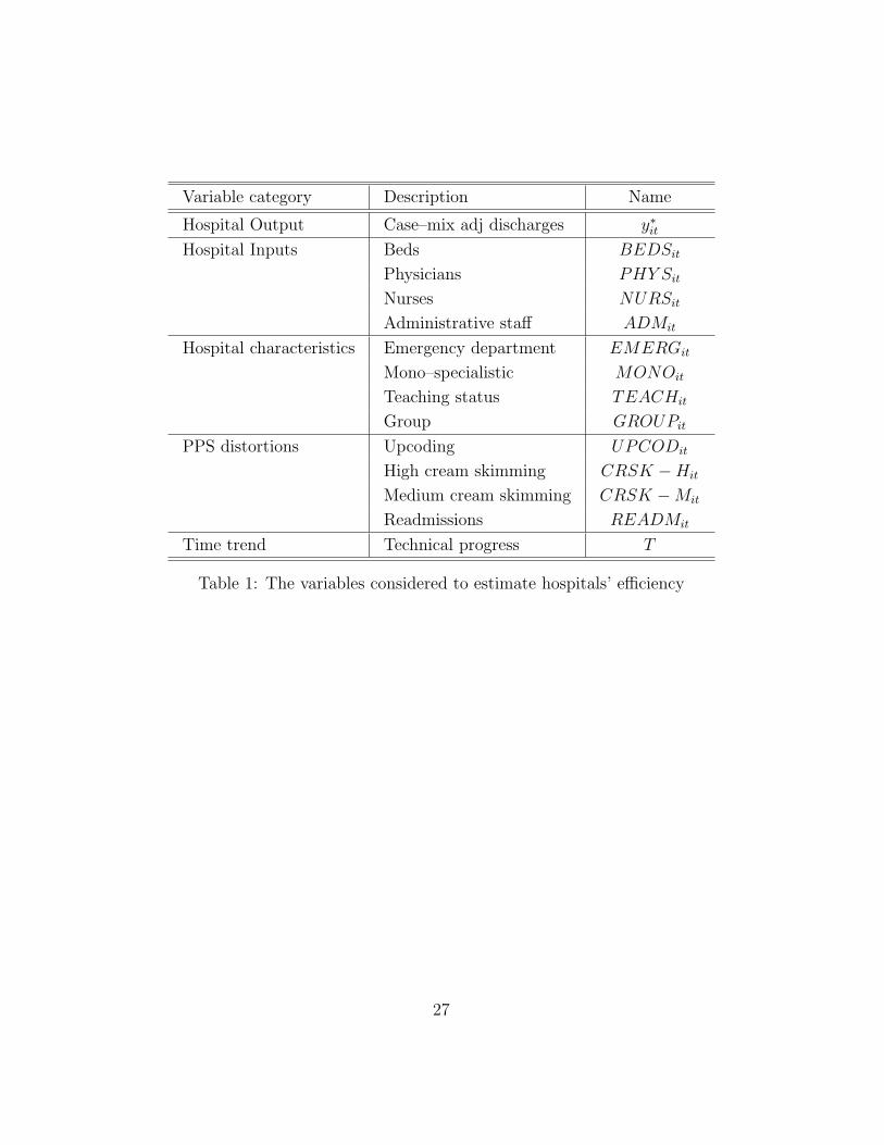
The variables we consider to estimate hospitals’ efficiency are shown in

Table 1. The hospitals’ output is the dependent variable. Following Cleverley

(2002), we consider the number of discharges adjusted both for case–mix and

for the weight of day–care and outpatient activities on the overall hospital

activity.13 Hence the hospital output is given by the following expression:

y∗it = yINit ×

(1 +

RDCit + ROUT

it

RINit

)× AW IN

it (6)

with y∗it being the total number of discharges case–mix adjusted, yINit the

total number of inpatient discharges, RDCit the day–care revenues, ROUT

it the

outpatient revenues, RINit the inpatient revenues and AWit the average DRG

weight for inpatient activity of hospital i at time t.

[Table 1 here]

The input variables concern beds (BEDS), hospital staff divided among

physicians (PHY S), nurses (NURS) and administrative staff (ADM).14

13The available dataset does not split the personnel utilization among inpatient, day–

care and outpatient activities. Hence it is necessary to consider an output that aggregates

all the hospital’s activities. Furthermore, during the observed period day–care and outpa-

tient activities have grown consistently; hence it is necessary to consider their weight in

the overall hospital output.14All labour variables are computed as full time equivalent employees. The information

does not include temporary workers, which may lead to an underestimation of this input,

particularly in private hospitals.

12

Moreover, we include some distinctive hospital features, such as the presence

of an emergency department (the dummy EMERG = 1 if the department

is present), the concentration of health services in the treatment of only one

pathology (the dummy MONO = 1 for cardiological, neurological, oncologic

and orthopaedic hospitals), the presence of a University within the hospital

(the dummy TEACH = 1 if the hospital has a university teaching status)

and the management of more than one hospital under the same authority

(the dummy GROUP = 1 if the hospital belongs to a group). The dis-

tribution of these variables in our sample is described in the next Section.

Furthermore, we consider the three distortions described before, i.e. upcod-

ing (UPCOD), high and medium cream skimming (CRSKH and CRSKM)

and readmissions (READM), and a time variable T representing the linear

trend in technological progress.15

Once we have estimated the hospitals’ efficiency score (which is time

invariant in the RE model and time variant in the TRE one), we analyze

the impact of ownership on efficiency. Following Singh and Coelli (2001)

we consider the estimated efficiency scores for public, private and private

not–for–profit hospitals and we apply the Kruskal–Wallis test to check for

significant differences.

As mentioned previously, we consider two functional forms for the pro-

duction frontier, a Cobb Douglas model and a Translog model. Under the

Cobb Douglas model, the equation we estimate is as follows:

log(y∗it) = α +4∑

j=1

βjlog(xjit) +4∑

l=1

γlzlit +4∑

k=1

δkdkit + ζT (7)

where xjit is the input j (i.e. beds, physicians, nurses and administrative

15Concerning the variable READM , the estimation has been performed with ∆=45

following the suggestions of the regional health care officers. In Lombardy Region, since

1998 the regional reimbursement system bears a reduction in the unit reimbursement in

case of a readmission within 45 days.

13

staff) in hospital i at period t, zlit is the characteristic l (i.e. the dummies

for the presence of an emergency department, of a mono–specialistic activity,

of a teaching activity and of belonging to a group) in hospital i at period

t, dkit is the level of distortion k (i.e. upcoding, the two dummies for cream

skimming and readmissions) in hospital i at period t and T is the time trend.

Furthermore, we also adopt a Translog functional form (see Christensen

et al. (1973)) for the production function, and in this case the model we

estimate is the following one:

log(y∗it) = α +4∑

j=1

βjlog(xjit) +1

2

4∑j=1

4∑h=1

βjhlog(xjit)log(xhit)+

+4∑

l=1

γlzlit +4∑

k=1

δkdkit + ζT

(8)

where, differently from the Cobb Douglas functional form displayed in ex-

pression (7), we also estimate both the possible interactions between the

hospital’s inputs and their second order effects. The results will be displayed

in Section 5.

4 The dataset

We investigate a large administrative dataset covering the full population of

patients and hospitals operating in the Lombardy Region, with over 20,000,000

admissions, between 1998 and 2007. Since our information come from ad-

ministrative data we can analyze our research questions over the entire pop-

ulation and not only over a sample; hence we do not incur in the sample

selection error component (Imai et al. (2008)).

The data are provided by the Health Care Department of the Lombardy

Region. We extracted the data concerning all the Hospital Discharge Charts,

which include information regarding the patient (gender, age, residence), the

hospital (regional code) and the admission (DRG, length of stay, principal

14

and secondary diagnosis–from which comorbidity is computed–, principal and

secondary procedures). This dataset has been linked with another database–

always provided by the Lombard Health Care Department–regarding all the

hospital’s features (beds, physicians, nurses, ownership, presence of emer-

gency unit, etc.).16

In 1997 there has been a deep institutional change in the Italian National

Health Service (NHS) that has resulted in a gradual re–balancing of respon-

sibilities, from the central system to the regions, in financing and organizing

health care services. Lombardy has been the first Region to implement,

through its 1997 Regional Health Reform Act, an innovative health care

model that favors competition among hospitals, with the aim to improve the

quality of health care services across the territory, to increase the patients

hospitals choice set, as well as to reduce health care costs. No major changes

have instead been implemented during the observed period.

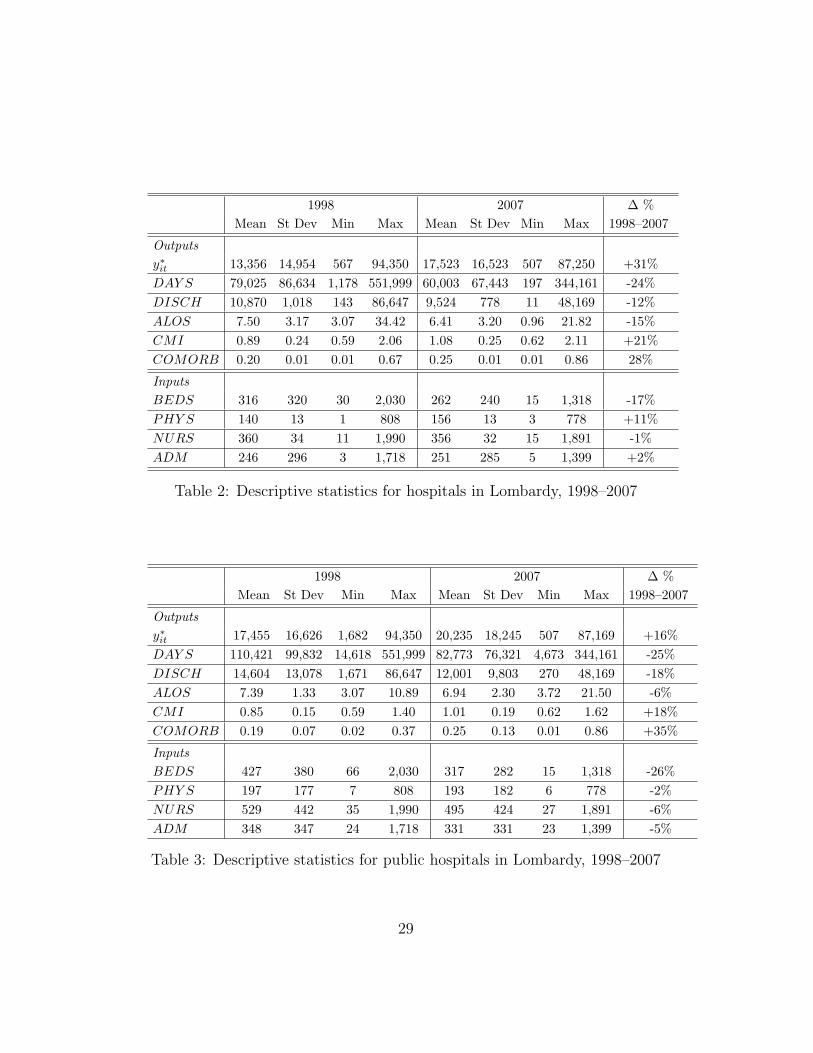
Table 2 shows some descriptive statistics concerning the whole dataset.

The total number of discharges adjusted for case–mix and for hospital activi-

ties (i.e. y∗it as defined in (6)) has increased during the period (+31%), as well

as the case–mix index (CMI +21%); on the contrary we observe a decrease

both in the length of stay (DAY S, -24%), in the average length of stay

(ALOS, -15%) and in the total number of inpatient discharges (DISCH,

-12%). This evidence is consistent with the insights reported in literature

concerning some general effects of the introduction of PPS (i.e. a reduction

in ALOS and number of discharges, compensated by an increase in the day–

care and outpatient treatments). Furthermore, we observe an increase in the

case–mix and a worsening of the patient health status: the comorbidity in-

dex (COMORB) increases by 28% during the period. Regarding inputs, the

16Information are recorded in Access. The data are not public under Italian privacy law.

The Health Care Department of the Lombardy Region may be contacted for discussing

the provision of the data with the aim of scientific publications.

15

total number of beds decreased over the period (-17%), showing that the sys-

tem was running in over–capacity at the beginning of the period. Among the

staff, nurses are the only staff category with a small decrease over the period

(-1%), while physicians show a robust increase (+11%). A small increase

(+2%) is observed for administrative staff. Italian hospitals have mainly

expanded the employment of physicians.

[Table 2 here]

In 2007 emergency units are active in 65% of hospital, while only 6% of

them can be classified as mono–specialistic organization. Academics activity

is performed by 10% of the hospitals and 60% of them are part of a group.

In the dataset, about 54% of the 134 hospitals active in Lombardy are

public (72), while about 34% are private (46). The remaining 12% is given by

not–for–profit organizations (16).17 The ownership distribution is constant

over the period, showing that no mergers and acquisitions among hospitals

(which are a frequent event in the US)18 are planned in Italy. The not–

for–profit hospitals are concentrated in the Milan county (60% of the total

not–for–profit ones); other hospitals of this ownership type are in the Como

county (20%), in Pavia (13%) and Brescia (7%). In the other Lombard coun-

ties there are no not–for–profit hospitals. Private hospitals are instead active

in all the Lombardy counties, as well as the public ones. The distribution

17We follow the classification adopted by Barbetta et al. (2007), and consider as public

both Aziende Ospedaliere (hospital enterprises) and Istituti di Ricovero e Cura a Carattere

Scientifico Pubblici (public research hospitals); we classify as not–for–profit hospitals both

Istituti di Ricovero e Cura a Carattere Scientifico Privati (private research hospitals) and

Ospedali Classificati (hospitals run by religious bodies); private hospitals are the private

accredited ones. As stated by Sloan (2000), the main distinction between private and

not–for–profit organization lies in the distribution of accounting profits. The latter do not

distribute such profit. Public hospital are controlled by the regional or local governments.18See Krishnan (2001) and Vita and Sacher (2001)

16

of private and public hospitals across the counties follows the population

distribution.

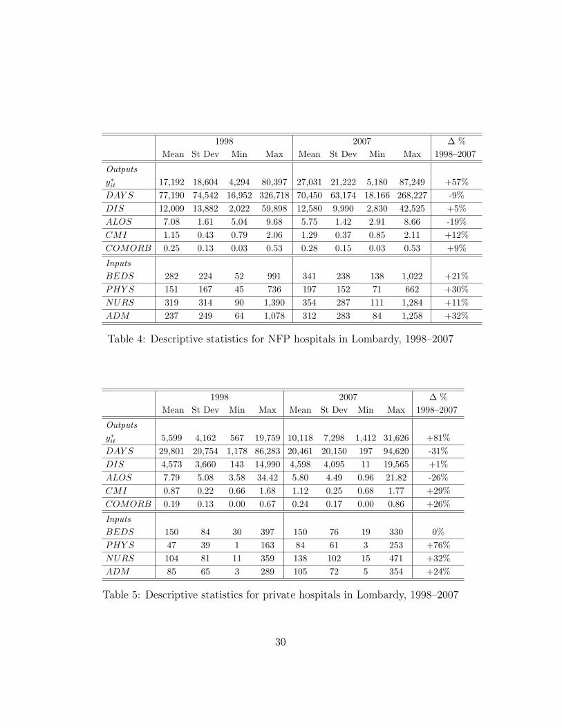
Table 3 presents the descriptive statistics regarding only the public hos-

pitals active in Lombardy during the observed period. Furthermore, Tables

4 and 5 display the same data, respectively, for not–for–profit and private

hospitals. It is interesting to point out that, while in 1998 public (private)

hospitals produced the highest (lowest) level of case–mix and activity–mix

adjusted output, at the end of the period not–for–profit hospitals registered

the highest output level (while private hospitals have always the lowest).

This swap is not observed if we focus on discharges; not–for–profit hospitals

have the highest case–mix index both at the beginning and at the end of

the period, while private ones have always the lowest. Not–for–profit hospi-

tals have also the highest comorbidity index; public hospitals have a higher

comorbidity index than private ones in 2007.

If we look at inputs, we observe that while public hospitals have the

highest number of beds and of physicians in 1998, not–for–profit ones register

the highest inputs’ levels in 2007. Private hospitals have always the lowest

number of beds and physicians. The largest number of nurses is always

observed in public hospital, as well as administrative staff. Private hospitals

have always the lowest employment level.

[Table 3 here]

[Table 4 here]

[Table 5 here]

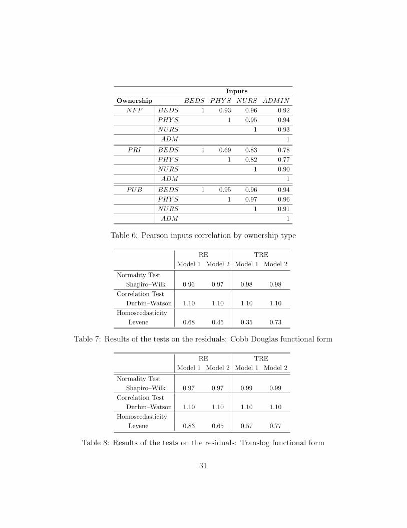
Table 6 displays the inputs Pearson correlation index for ownership type.

While there is a high positive correlation between beds and the different

staff types (and among the number of physicians, nurses and administrative

staff) in not–for–profit and public hospitals, the correlation between beds

17

and physicians is only 0.69 in private ones. The correlation between beds

and nurses is 0.83 in private hospitals, and between beds and administrative

staff is only 0.78. Moreover the correlation indices among staff are always

lower than those observed in the other two hospital types. All these data

suggest that private not–for-profit hospitals are very similar to public ones,

while private hospitals are smaller and with a lower employment/beds ratio.

[Table 6 here]

5 Results

In this Section we present the results of the empirical analysis. We split the

evidence in two parts. First (5.1) we display some descriptive statistics about

the distribution of the three distortions for ownership type. Second (5.2), we

present the estimates of the efficient frontier and the impact of the distortions

on hospitals’ output and we test whether there exists an ownership ranking

according to the estimated efficiency scores.19

5.1 The distribution of PPS across hospitals with different own-

ership

We now present some empirical evidence concerning the distribution of the

three PPS distortions in not–for–profit, private and public hospitals, and

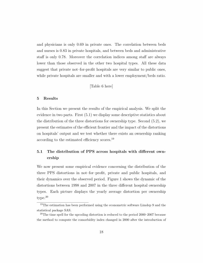
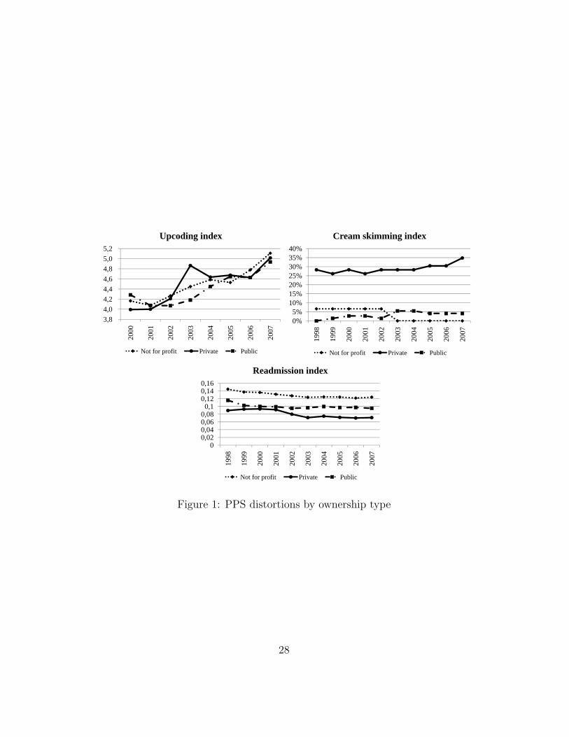
their dynamics over the observed period. Figure 1 shows the dynamic of the

distortions between 1998 and 2007 in the three different hospital ownership

types. Each picture displays the yearly average distortion per ownership

type.20

19The estimation has been performed using the econometric software Limdep 9 and the

statistical package SAS.20The time spell for the upcoding distortion is reduced to the period 2000–2007 because

the method to compute the comorbidity index changed in 2000 after the introduction of

18

[Figure 1 here]

It is evident that the behavior of the three hospital types regarding the

distortions is heterogeneous.21 The three hospital types demonstrate a rather

uniform behavior concerning upcoding, differently from Silverman and Skin-

ner (2004) and Dafny (2005), who reported a higher upcoding activity in

private hospitals. In our dataset private hospitals were more engaged in

this practice only during the period 2003–2005. In the remaining years their

behavior was similar to that of the other hospitals. Moreover, we observe

an increasing trend in this distortion and a convergence among the different

ownership types during the period of investigation.22

The index for treatment cream skimming is much higher for private hos-

pitals, while this distortion is small in not–for–profit and public hospitals.

Moreover, the convergence between the two latter types seems to increase

with time and their activity concerning this distortion seems to decrease.

This new insight confirms some expectations among the profession (i.e. pri-

vate hospitals do select the treatments), but it is the first attempt to quantify

them. Another interesting result is that not–for–profit and public hospitals

exhibit the same very low level of treatment cream skimming.23

Figure 1 also shows the general trend for the readmission distortion.

All the indices decrease over the period. Not–for–profit hospitals produce

the 14th version of the DRG Grouper, and this modification does not allow to compare

the statistics for 1998–1999 with the remaining years.21We have performed Kruskal–Wallis tests for difference in the mean, which confirm the

behavioral distinctions reported here.22The spike observed for private hospitals in 2003 is due to a change in the reimbursement

method that may have allowed a higher upcoding activity during that year. More severe

checks implemented after 2003 by regional health officers have limited this chance.23This evidence is different from Sloan (2000), which argues that for–profit and not–

for–profit hospitals are far more alike than different. It is closer to Silverman and Skinner

(2004), and the difference between for–profit and not–for–profit hospitals may be due to

the presence of altruism (Newhouse (1970)) and vocational purposes.

19

a higher distortion, while the private ones show the lowest level. We provide

two possible explanations for this evidence: (1) More severe controls on the

activity of private hospitals on this distortion, which may be more easily

checked by the regulator than the previous ones. (2) As mentioned pre-

viously, two effects could have an impact on readmissions: reputation and

opportunistic behavior. The reputation effect may be stronger if we con-

sider not–for–profit and public hospitals (see Newhouse (1970), Hansmann

(1980)): they have more readmissions because of a better reputation. The

latter induces a highest share of less healthy patients, which require repeated

and more frequent treatments.

5.2 The estimates of technical efficiency for Italian hospitals

In this Section we present the estimates of efficiency for Italian hospitals and

we observe whether there is a difference according to the ownership types.

As mentioned previously, for each functional form, i.e. Cobb Douglas and

Translog, we estimated two econometric specifications: the RE model and

the TRE model. Moreover, for each functional form and for each econometric

specification, we performed two different regressions including different sets

of covariates: Model 1 considers only input variables, hospital characteristics

(i.e. presence of emergency department, specialization, etc.) and the time

trend, while Model 2 includes also the proxies for the distortions.

The Shapiro and Wilk (1965) normality test on the dependent variable

(i.e. the case–mix adjusted discharges) shows that there is no evidence of non–

normality of this sample (see Tables 7–8).24 Moreover, the Levene test shows

that the residuals are homoscedastic.25 The Durbin–Watson test reveals a

24The p–values associated with the W statistic are higher than the critical value of 0.01;

thus as stated by Shapiro and Wilk (1965) p. 606, “there is no evidence of non–normality

of this sample”.25The p–values associated to the Levene statistic are higher than the critical value of

20

lack of correlation among the residuals.26 Finally, the Variance Inflation

Factor (VIF) index for input multicollinearity shows that inputs are not

influenced by multicollinearity.27

[Table 7 here]

[Table 8 here]

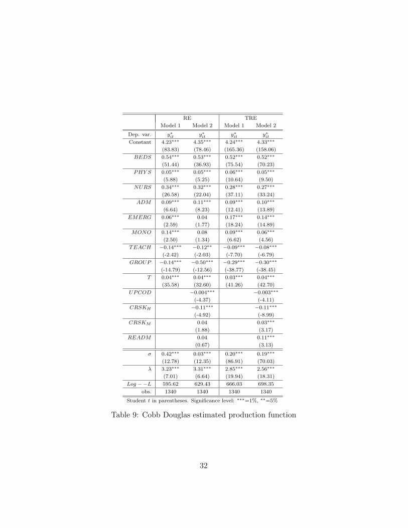
The econometric results shown in Tables 9 and 10 are robust to the dif-

ferent specifications, with very few exceptions. In all the models the input

variables are highly significant with positive coefficients, with the exception

of administrative staff under the Translog functional form.28

[Table 9 here]

[Table 10 here]

Regarding hospital’s characteristics, the presence of an emergency depart-

ment increases the efficiency under both econometric models. It seems that,

by having emergency unit, hospitals are able to admit more patients, and of-

ten the more complicated ones. As expected, mono–specialistic hospitals are

more efficient than multi–specialist ones. The presence of academics activity

within the hospitals has a negative impact on the production frontier under

0.01; thus we can accept the null hypothesis of homoscedasticity.26The Durbin–Watson test signals correlation among the residuals if the statistics as-

sumes values D ≤ 1 or D ≥ 3.27The VIF indexes are the following: VIF(log(BEDS))=6.53, VIF(log(MED))=8.73

and VIF(log(ADM))=7.31. The rule proposed by Kutner et al. (2004) is that a value of

V IF ≥ 10 is an indication of potential multicollinearity problems.28The two input variables having the highest impact on the hospitals’ output are the

number of beds and nurses in the Cobb Douglas models, while physicians have the lowest

coefficient. In the RE model the sum of the input coefficients is consistent with increasing

returns to scale, while in the TRE model we observe decreasing returns to scale.

21

the Cobb Douglas functional form, while there is no statistically significant

effect under the Translog model. If more than one hospital is controlled by

the same authority production is lower: analyzed hospitals have some diffi-

culties to deal with multiplant technologies. The sign of the time variable,

capturing the shift in technology, shows an increase in the production frontier

over the observed period.

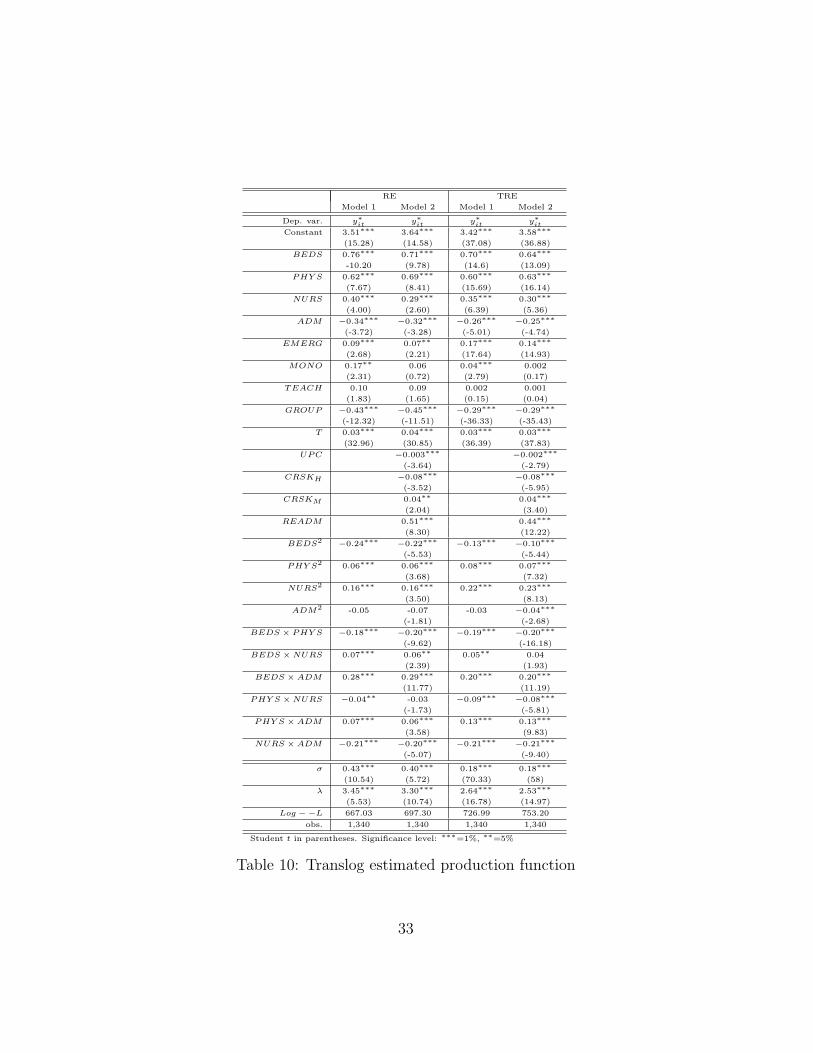
Table 10 presents the estimated production function for the Translog

functional form. In general all the previous results are replicated; the second

order and interaction terms are almost completely statistically significant. A

negative coefficient is observed for the interaction between beds and physi-

cians, physicians and nurses and nurses and administrative staff. A positive

interaction is instead estimated for beds and nurses, beds and administrative

staff and physicians and administrative staff.

Last, we analyze the impact on hospitals’ efficiency of the three distor-

tions. Upcoding and treatment cream skimming reduce the hospitals’ ef-

ficiency in all the models. This means that hospitals with high upcoding

either suffer of a Leibenstein X–inefficiency factor since they obtain higher

revenues thanks to the distortions (see Leibenstein (1966)), or they choose to

treat less cases to justify the presence of treatments with high DRG weights.29

Regarding treatment cream skimming, again the possible explanations may

be a Leibenstein X–inefficiency factor and the lower number of discharges

due to treatment selection (i.e. the management chooses to focus the activity

on some treatments but this effect is not compensated by the reduction in

discharges due to the restriction in the number of DRGs treated).

29Leibenstein introduces the theory of inefficiency generated from non–competition. It

may be summarized as follows: “For a variety of reasons people and organizations normally

work neither as hard or as effectively as they could. In situations where competitive

pressure is light, many people will trade the disutility of greater effort, or search for the

utility of feeling less pressure and of better interpersonal relations.” Essentially, there will

be a slack in cost control and in the amount of effort put in by management and workers.

22

Readmissions have a strong positive impact on efficiency, because, as

expected, this practice increases the hospital’s output; however, it might be

that this is due to an opportunistic behavior (not to an efficiency effect).

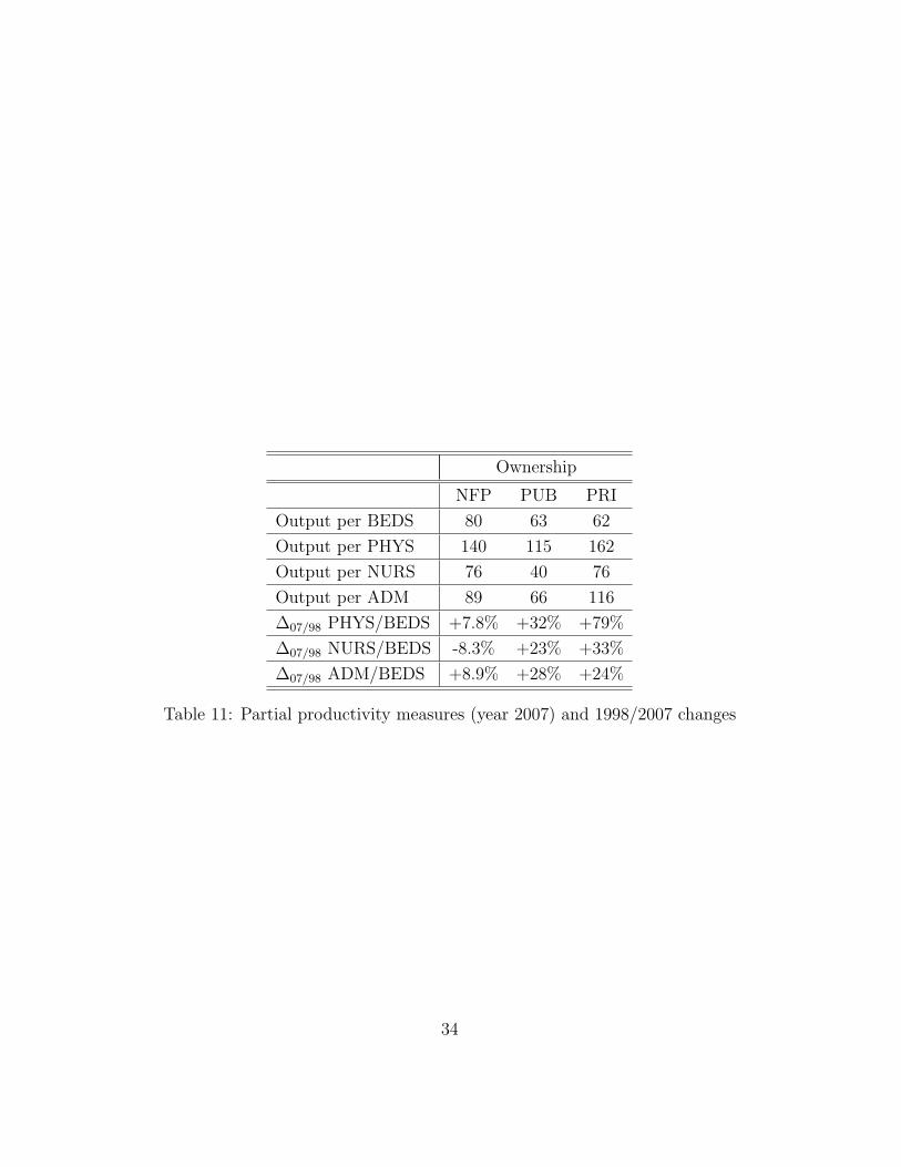
We can now analyze the efficiency ranking according to the hospital own-

ership. If we compute the partial productivity measures (see Table 11), i.e.

output produced per input, we observe that private hospitals have the largest

values for physicians, nurses and administrative staff, while public structures

have the lowest measures. On the contrary, the ranking is the opposite if we

consider beds.

[Table 11 here]

A more robust analysis can be performed using the estimated efficiency

scores. Table 12 shows the average estimated efficiency score for public, not–

for–profit and private hospitals under the two econometric models and for

the Translog functional form (the same results hold for the Cobb Douglas

function form). We consider the efficiency scores (i.e. Exp(−ui), ui ≥ 0)

estimated using only the inputs as covariates.

Under the RE model–where a time invariant efficiency score is estimated

for each hospital–the average efficiency score of public hospitals is greater

than that of not–for–profit hospitals; the lowest average is for private ones.

Table 12 also displays the Kruskal–Wallis test for statistically significant dif-

ferences in the ownership average efficiency scores. Based on these tests,

the null hypothesis of no difference between the technical efficiency scores of

the two ownership types is investigated. Under the RE model the null hy-

pothesis is rejected only for public and private hospitals, i.e. public hospitals

are statistically more efficient than private ones. No statistically significant

difference is observed between public and not–for–profit hospitals.

Hence public hospitals are technically more efficient than private ones,

as shown by Puig–Junoy (1998) for Spanish hospitals and Zuckerman et al.

23

(1994) for the US ones, and differently from Wilson and Jadlow (1982). This

ranking can be explained by considering the estimated input coefficients,

the partial productivity measures and the inputs correlation across owner-

ship types. Private hospitals have the lowest partial productivity measure

for beds, which is the input with the largest coefficient in the estimated

production frontier. For these reasons they have the lowest ranking in tech-

nical efficiency. If we consider that private hospitals exhibit also the lowest

correlation between beds and personnel, this implies that they employ less

physicians, nurses and administrative staff per beds. This is probably the

strategy adopted by managers of private hospitals to reduce labour costs.

If we consider the TRE model, where a time–variant efficiency score is

estimated, we can observe whether there are any ownership differences in

the efficiency trends. We find that at the beginning of the period public and

not–for–profit hospitals are more efficient than private ones. On the contrary,

at the end of the period (year 2007) no significant difference among the

average efficiency scores of the three ownership types is observed (as shown

by Vitaliano and Toren (1996), Sloan (2000) and Barbetta et al. (2007)).

Hence the regional system has became more uniform according to technical

efficiency estimates. This is probably due to a more stringent regulation,

since the fulfillments required in order to be part of the mixed health care

regional system have been tightened over the period.

[Table 12 here]

6 Conclusions

This paper provides some indices to measure three typical PPS distortions:

upcoding, treatment cream skimming and readmissions. Moreover, these

distortions are introduced as covariates to investigate the efficiency of Italian

hospitals.

24

The main results are the following. First, readmissions are the most

relevant distortion, since they significantly increase hospitals’ output. Sec-

ond, cream skimming and upcoding have a negative impact on efficiency.

Third, private hospitals are particularly engaged in treatment cream skim-

ming, while this distortion is very low in public and not–for–profit hospi-

tals. Fourth, no ownership differences are observed if we look at upcoding

(differently from Silverman and Skinner (2004) and Dafny (2005)), while

not–for–profit hospitals make more readmissions than public hospitals, and

the private ones have very low indices. Fifth, not–for–profit and public hos-

pitals show a similar technical efficiency level, and are more efficient than

private ones at the beginning of the observed period, while no differences are

observed at the end of the period.

We can draw some policy implications from the above results. First,

since upcoding and cream skimming have a negative impact on efficiency, the

policy maker may anticipate that hospitals with high upcoding and cream

skimming indices have some spare capacity (e.g. too many beds) or more

personnel than that required under technical efficiency. This inefficient re-

sources’ utilization is due to the management’s decision to specialize in the

most lucrative treatments. Hence we suggest that the policy maker should

use the incentive mechanism in order to try to correct these distortions. One

possibility could be the adoption of a reimbursement scheme where the price

paid for DRGs with complications (which may be affected by upcoding) is

inversely related to the level of the distortion.

Second, hospitals with high readmission index use all the available inputs,

since readmissions have a positive impact on technical efficiency. However,

they adopt an opportunistic behavior to increase the total reimbursement.

In this case the policy maker should rise the penalty reduction in the re-

imbursement rate (already implemented in the regional health care service

we analyzed) in case of a readmission occurred in the same hospital, for the

25

same DRG and shortly after the first admission.

This paper is a first attempt to estimate the impact of some distortions

induced by the PPS on technical efficiency. Further research is needed on

designing better indices to estimate the distortions (and to include others,

e.g. early discharges), and to identify the determinants of the opportunistic

behavior. Furthermore, it is necessary to extend the analysis to hospital’s

costs and revenues, to identify whether the PPS has achieved the goal of costs

containment and if there a different ranking among the different ownership

structures. Last, different regional systems may be considered to control for

cross–regional differences.

26

Variable category Description Name

Hospital Output Case–mix adj discharges y∗itHospital Inputs Beds BEDSit

Physicians PHY Sit

Nurses NURSit

Administrative staff ADMit

Hospital characteristics Emergency department EMERGit

Mono–specialistic MONOit

Teaching status TEACHit

Group GROUPit

PPS distortions Upcoding UPCODit

High cream skimming CRSK −Hit

Medium cream skimming CRSK −Mit

Readmissions READMit

Time trend Technical progress T

Table 1: The variables considered to estimate hospitals’ efficiency

27

5,2

Upcoding index40%

Cream skimming index

4 44,6 4,8 5,0

20%25%30%35%

3,8 4,0 4,2 4,4

0%5%

10%15%

,

2000

2001

2002

2003

2004

2005

2006

2007

Not for profit Private Public

0%19

98

1999

2000

2001

2002

2003

2004

2005

2006

2007

Not for profit Private Public

0,140,16

Readmission index

0 040,060,08

0,10,120,14

00,020,04

1998

1999

2000

2001

2002

2003

2004

2005

2006

2007

1 1 2 2 2 2 2 2 2 2

Not for profit Private Public

Figure 1: PPS distortions by ownership type

28

1998 2007 ∆ %Mean St Dev Min Max Mean St Dev Min Max 1998–2007

Outputsy∗it 13,356 14,954 567 94,350 17,523 16,523 507 87,250 +31%DAY S 79,025 86,634 1,178 551,999 60,003 67,443 197 344,161 -24%DISCH 10,870 1,018 143 86,647 9,524 778 11 48,169 -12%ALOS 7.50 3.17 3.07 34.42 6.41 3.20 0.96 21.82 -15%CMI 0.89 0.24 0.59 2.06 1.08 0.25 0.62 2.11 +21%COMORB 0.20 0.01 0.01 0.67 0.25 0.01 0.01 0.86 28%

InputsBEDS 316 320 30 2,030 262 240 15 1,318 -17%PHY S 140 13 1 808 156 13 3 778 +11%NURS 360 34 11 1,990 356 32 15 1,891 -1%ADM 246 296 3 1,718 251 285 5 1,399 +2%

Table 2: Descriptive statistics for hospitals in Lombardy, 1998–2007

1998 2007 ∆ %Mean St Dev Min Max Mean St Dev Min Max 1998–2007

Outputsy∗it 17,455 16,626 1,682 94,350 20,235 18,245 507 87,169 +16%DAY S 110,421 99,832 14,618 551,999 82,773 76,321 4,673 344,161 -25%DISCH 14,604 13,078 1,671 86,647 12,001 9,803 270 48,169 -18%ALOS 7.39 1.33 3.07 10.89 6.94 2.30 3.72 21.50 -6%CMI 0.85 0.15 0.59 1.40 1.01 0.19 0.62 1.62 +18%COMORB 0.19 0.07 0.02 0.37 0.25 0.13 0.01 0.86 +35%

InputsBEDS 427 380 66 2,030 317 282 15 1,318 -26%PHY S 197 177 7 808 193 182 6 778 -2%NURS 529 442 35 1,990 495 424 27 1,891 -6%ADM 348 347 24 1,718 331 331 23 1,399 -5%

Table 3: Descriptive statistics for public hospitals in Lombardy, 1998–2007

29

1998 2007 ∆ %Mean St Dev Min Max Mean St Dev Min Max 1998–2007

Outputsy∗it 17,192 18,604 4,294 80,397 27,031 21,222 5,180 87,249 +57%DAY S 77,190 74,542 16,952 326,718 70,450 63,174 18,166 268,227 -9%DIS 12,009 13,882 2,022 59,898 12,580 9,990 2,830 42,525 +5%ALOS 7.08 1.61 5.04 9.68 5.75 1.42 2.91 8.66 -19%CMI 1.15 0.43 0.79 2.06 1.29 0.37 0.85 2.11 +12%COMORB 0.25 0.13 0.03 0.53 0.28 0.15 0.03 0.53 +9%

InputsBEDS 282 224 52 991 341 238 138 1,022 +21%PHY S 151 167 45 736 197 152 71 662 +30%NURS 319 314 90 1,390 354 287 111 1,284 +11%ADM 237 249 64 1,078 312 283 84 1,258 +32%

Table 4: Descriptive statistics for NFP hospitals in Lombardy, 1998–2007

1998 2007 ∆ %Mean St Dev Min Max Mean St Dev Min Max 1998–2007

Outputsy∗it 5,599 4,162 567 19,759 10,118 7,298 1,412 31,626 +81%DAY S 29,801 20,754 1,178 86,283 20,461 20,150 197 94,620 -31%DIS 4,573 3,660 143 14,990 4,598 4,095 11 19,565 +1%ALOS 7.79 5.08 3.58 34.42 5.80 4.49 0.96 21.82 -26%CMI 0.87 0.22 0.66 1.68 1.12 0.25 0.68 1.77 +29%COMORB 0.19 0.13 0.00 0.67 0.24 0.17 0.00 0.86 +26%

InputsBEDS 150 84 30 397 150 76 19 330 0%PHY S 47 39 1 163 84 61 3 253 +76%NURS 104 81 11 359 138 102 15 471 +32%ADM 85 65 3 289 105 72 5 354 +24%

Table 5: Descriptive statistics for private hospitals in Lombardy, 1998–2007

30

InputsOwnership BEDS PHY S NURS ADMIN

NFP BEDS 1 0.93 0.96 0.92PHY S 1 0.95 0.94NURS 1 0.93ADM 1

PRI BEDS 1 0.69 0.83 0.78PHY S 1 0.82 0.77NURS 1 0.90ADM 1

PUB BEDS 1 0.95 0.96 0.94PHY S 1 0.97 0.96NURS 1 0.91ADM 1

Table 6: Pearson inputs correlation by ownership type

RE TREModel 1 Model 2 Model 1 Model 2

Normality TestShapiro–Wilk 0.96 0.97 0.98 0.98

Correlation TestDurbin–Watson 1.10 1.10 1.10 1.10

HomoscedasticityLevene 0.68 0.45 0.35 0.73

Table 7: Results of the tests on the residuals: Cobb Douglas functional form

RE TREModel 1 Model 2 Model 1 Model 2

Normality TestShapiro–Wilk 0.97 0.97 0.99 0.99

Correlation TestDurbin–Watson 1.10 1.10 1.10 1.10

HomoscedasticityLevene 0.83 0.65 0.57 0.77

Table 8: Results of the tests on the residuals: Translog functional form

31

RE TRE

Model 1 Model 2 Model 1 Model 2

Dep. var. y∗it y∗it y∗it y∗itConstant 4.23∗∗∗ 4.35∗∗∗ 4.24∗∗∗ 4.33∗∗∗

(83.83) (78.46) (165.36) (158.06)

BEDS 0.54∗∗∗ 0.53∗∗∗ 0.52∗∗∗ 0.52∗∗∗

(51.44) (36.93) (75.54) (70.23)

PHY S 0.05∗∗∗ 0.05∗∗∗ 0.06∗∗∗ 0.05∗∗∗

(5.88) (5.25) (10.64) (9.50)

NURS 0.34∗∗∗ 0.32∗∗∗ 0.28∗∗∗ 0.27∗∗∗

(26.58) (22.04) (37.11) (33.24)

ADM 0.09∗∗∗ 0.11∗∗∗ 0.09∗∗∗ 0.10∗∗∗

(6.64) (8.23) (12.41) (13.89)

EMERG 0.06∗∗∗ 0.04 0.17∗∗∗ 0.14∗∗∗

(2.59) (1.77) (18.24) (14.89)

MONO 0.14∗∗∗ 0.08 0.09∗∗∗ 0.06∗∗∗

(2.50) (1.34) (6.62) (4.56)

TEACH −0.14∗∗∗ −0.12∗∗ −0.09∗∗∗ −0.08∗∗∗

(-2.42) (-2.03) (-7.70) (-6.79)

GROUP −0.14∗∗∗ −0.50∗∗∗ −0.29∗∗∗ −0.30∗∗∗

(-14.79) (-12.56) (-38.77) (-38.45)

T 0.04∗∗∗ 0.04∗∗∗ 0.03∗∗∗ 0.04∗∗∗

(35.58) (32.60) (41.26) (42.70)

UPCOD −0.004∗∗∗ −0.003∗∗∗

(-4.37) (-4.11)

CRSKH −0.11∗∗∗ −0.11∗∗∗

(-4.92) (-8.99)

CRSKM 0.04 0.03∗∗∗

(1.88) (3.17)

READM 0.04 0.11∗∗∗

(0.67) (3.13)

σ 0.42∗∗∗ 0.03∗∗∗ 0.20∗∗∗ 0.19∗∗∗

(12.78) (12.35) (86.91) (70.03)

λ 3.23∗∗∗ 3.31∗∗∗ 2.85∗∗∗ 2.56∗∗∗

(7.01) (6.64) (19.94) (18.31)

Log −−L 595.62 629.43 666.03 698.35

obs. 1340 1340 1340 1340

Student t in parentheses. Significance level: ∗∗∗=1%, ∗∗=5%

Table 9: Cobb Douglas estimated production function

32

RE TRE

Model 1 Model 2 Model 1 Model 2

Dep. var. y∗it y∗it y∗it y∗itConstant 3.51∗∗∗ 3.64∗∗∗ 3.42∗∗∗ 3.58∗∗∗

(15.28) (14.58) (37.08) (36.88)

BEDS 0.76∗∗∗ 0.71∗∗∗ 0.70∗∗∗ 0.64∗∗∗

-10.20 (9.78) (14.6) (13.09)

PHY S 0.62∗∗∗ 0.69∗∗∗ 0.60∗∗∗ 0.63∗∗∗

(7.67) (8.41) (15.69) (16.14)

NURS 0.40∗∗∗ 0.29∗∗∗ 0.35∗∗∗ 0.30∗∗∗

(4.00) (2.60) (6.39) (5.36)

ADM −0.34∗∗∗ −0.32∗∗∗ −0.26∗∗∗ −0.25∗∗∗

(-3.72) (-3.28) (-5.01) (-4.74)

EMERG 0.09∗∗∗ 0.07∗∗ 0.17∗∗∗ 0.14∗∗∗

(2.68) (2.21) (17.64) (14.93)

MONO 0.17∗∗ 0.06 0.04∗∗∗ 0.002

(2.31) (0.72) (2.79) (0.17)

TEACH 0.10 0.09 0.002 0.001

(1.83) (1.65) (0.15) (0.04)

GROUP −0.43∗∗∗ −0.45∗∗∗ −0.29∗∗∗ −0.29∗∗∗

(-12.32) (-11.51) (-36.33) (-35.43)

T 0.03∗∗∗ 0.04∗∗∗ 0.03∗∗∗ 0.03∗∗∗

(32.96) (30.85) (36.39) (37.83)

UPC −0.003∗∗∗ −0.002∗∗∗

(-3.64) (-2.79)

CRSKH −0.08∗∗∗ −0.08∗∗∗

(-3.52) (-5.95)

CRSKM 0.04∗∗ 0.04∗∗∗

(2.04) (3.40)

READM 0.51∗∗∗ 0.44∗∗∗

(8.30) (12.22)

BEDS2 −0.24∗∗∗ −0.22∗∗∗ −0.13∗∗∗ −0.10∗∗∗

(-5.53) (-5.44)

PHY S2 0.06∗∗∗ 0.06∗∗∗ 0.08∗∗∗ 0.07∗∗∗

(3.68) (7.32)

NURS2 0.16∗∗∗ 0.16∗∗∗ 0.22∗∗∗ 0.23∗∗∗

(3.50) (8.13)

ADM2 -0.05 -0.07 -0.03 −0.04∗∗∗

(-1.81) (-2.68)

BEDS × PHY S −0.18∗∗∗ −0.20∗∗∗ −0.19∗∗∗ −0.20∗∗∗

(-9.62) (-16.18)

BEDS × NURS 0.07∗∗∗ 0.06∗∗ 0.05∗∗ 0.04

(2.39) (1.93)

BEDS × ADM 0.28∗∗∗ 0.29∗∗∗ 0.20∗∗∗ 0.20∗∗∗

(11.77) (11.19)

PHY S × NURS −0.04∗∗ -0.03 −0.09∗∗∗ −0.08∗∗∗

(-1.73) (-5.81)

PHY S × ADM 0.07∗∗∗ 0.06∗∗∗ 0.13∗∗∗ 0.13∗∗∗

(3.58) (9.83)

NURS × ADM −0.21∗∗∗ −0.20∗∗∗ −0.21∗∗∗ −0.21∗∗∗

(-5.07) (-9.40)

σ 0.43∗∗∗ 0.40∗∗∗ 0.18∗∗∗ 0.18∗∗∗

(10.54) (5.72) (70.33) (58)

λ 3.45∗∗∗ 3.30∗∗∗ 2.64∗∗∗ 2.53∗∗∗

(5.53) (10.74) (16.78) (14.97)

Log −−L 667.03 697.30 726.99 753.20

obs. 1,340 1,340 1,340 1,340

Student t in parentheses. Significance level: ∗∗∗=1%, ∗∗=5%

Table 10: Translog estimated production function

33

Ownership

NFP PUB PRI

Output per BEDS 80 63 62

Output per PHYS 140 115 162

Output per NURS 76 40 76

Output per ADM 89 66 116

∆07/98 PHYS/BEDS +7.8% +32% +79%

∆07/98 NURS/BEDS -8.3% +23% +33%

∆07/98 ADM/BEDS +8.9% +28% +24%

Table 11: Partial productivity measures (year 2007) and 1998/2007 changes

34

Average efficiency scores

Ownership RE TRE

1998 2007

Not–for–profit 0.73 0.86 0.87

Private 0.68 0.78 0.85

Public 0.76 0.87 0.87

Kruskal–Wallis tests

RE model

Hypothesis P–value Critical value Decision

TEPRI = TENFP 0.51 0.05 Accepted

TEPRI = TEPUB 0.003 0.05 Rejected

TEPUB = TENFP 0.53 0.05 Accepted

TRE model–year 1998

Hypothesis P–value Critical value Decision

TEPRI = TENFP 0.03 0.05 Rejected

TEPRI = TEPUB 0.00 0.05 Rejected

TEPUB = TENFP 0.52 0.05 Accepted

TRE model–year 2007

Hypothesis P–value Critical value Decision

TEPRI = TENFP 0.85 0.05 Accepted

TEPRI = TEPUB 0.18 0.05 Accepted

TEPUB = TENFP 0.20 0.05 Accepted

Table 12: Average efficiency scores and Kruskal–Wallis test significance for

ownership types

35

References

• Agency for Healthcare Research and Quality, 2008, Healthcare Cost

and Utilization Project, Comorbidity Software Version 3.3, http://www.hcup-

us.ahrq.gov/toolssoftware/comorbidity/comorbidity.jsp.

• Aigner, D.J., Lovell, C.A.K. and P. Schmidt, 1977, Formulation and

Estimation of Stochastic Frontier Production Function Models, Journal

of Econometrics, 6, 21–37.

• Barbetta, G.P., Turati, G. and A.M. Zago, 2007, Behavioral differ-

ences between public and private not–for–profit hospitals in the Italian

national health service, Health economics, 16, 75–96.

• Barros, P., 2003, Cream-skimming, incentives for efficiency and pay-

ment system, Journal of Health Economics, 22, 419–443.

• Charlson, M.E., Pompei, P., Ales, K.A. and C.R. MacKenzie, 1987,

A new method of classifying prognostic comorbidity in longitudinal

studies: development and validation, Journal of Chronic Diseases, 40,

373–383.

• Cleverley, W.O., 2002, The hospital cost index: A new way to assess

relative cost-efficiency, Healthcare Financial Management.

• Christensen, L., Jorgenson, D. and L. Lau, 1973, Transcendental loga-

rithmic production frontiers, The Review of Economics and Statistics,

55, 28–45.

36

• Cutler, D.M., 1995, The incidence of adverse medical outcomes under

prospective payment, Econometrica, 63, 29–50.

• Dafny, L.S., 2005, How do hospitals respond to price changes?, Amer-

ican Economic Review, 95, 1525–1547.

• de Groot, V., Beckerman, H., Lankhorst, G. and L. Bouter, 2003, How

to measure comorbidity: a critical review of available methods, Journal

of Clinical Epidemiology, 56, 221-229.

• Elixhauser, A., Steiner, C., Harris, D.R., and R.M. Coffey, 1998, Co-

morbidity measures for use with administrative data, Medical Care, 36,

8–27.

• Ellis, R.P., 1998, Creaming, skimping and dumping: provider compe-

tition on the intensive and extensive margins, Journal of Health Eco-

nomics, 17, 537-555.

• Imai, K., King, G. and E.A. Stuart, 2008, Misunderstandings between

experimentalists and observationalists about causal inference, Journal

of the Royal Statistical Society: Series A, 171, 481–502.

• Greene W., 2005a, Fixed and random effects in stochastic frontier mod-

els, Journal of Productivity Analysis, 23, 7-32.

• Greene, W., 2005b, Reconsidering heterogeneity and inefficiency: al-

ternative estimators for stochastic frontier models, Journal of Econo-

metrics, 126, 269–303.

• Hansmann, H.B., 1980. The role of nonprofit enterprise, Yale Law

Review, 89, 835901.

37

• Hollingsworth, B., 2003, Non–parametric and parametric applications

measuring efficiency in health care, Health Care Management Science,

6, 203-218.

• Krishnan, R., 2001, Market restructuring and pricing in the hospital

industry, Journal of Health Economics, 20, 213–237.

• Kutner, M., Nachtsheim, C. and J. Neter, 2004, Applied Linear Regres-

sion Models, 4th edition, McGraw-Hill Irwin.

• Levaggi, R. and Montefiori, M., 2003, Horizontal and vertical cream

skimming in the health care market, DISEFIN Working Paper No.

11/2003, Available at SSRN: http://ssrn.com/abstract=545583

• Leibenstein, H., 1966, Allocative efficiency vs “X–efficiency”, American

Economic Review, 56, 392–415.

• Louis, D.Z., Yuen, E.J., Braga, M., Cicchetti, A., Rabinowitz, C.,

Laine, C. and J.S. Gonnella, 1999, Impact of a DRG–based hospital

financing system on quality and outcomes of care in Italy, Health Ser-

vices Research, 34, 405-415.

• Newhouse, J., 1970. Towards a theory of non–profit institutions: an

economic model of a hospital, American Economic Review, 60, 64-74.

• Pitt, M., Lee, L., 1981, The measurement and sources of technical

inefficiency in the Indonesian weaving industry, Journal of Development

Economics, 9, 43-64.

• Puig–Junoy, J., 1998, Technical efficiency in the clinical management

of critically ill patients, Health Economics, 7, 263–277.

38

• Rosko, M.D., Mutter, R.L., Stochastic frontier analysis of hospital in-

efficiency: a review of empirical issues and an assessment of robustness,

Medical Care Research and Review, 65, 131-166.

• Shapiro, S.S. and M.B. Wilk, 1965, An analysis of variance test for

normality (complete samples), Biometrika, 52, 591-611.

• Silverman, E., Skinner, J., 2004, Medicare upcoding and hospital own-

ership, Journal of Health Economics, 23, 369–389.

• Simborg, D.W., 1981, DRG creep: a new hospital–acquired disease,

The New England Journal of Medicine, 304(26), 1602–1604.

• Singh, S., Coelli, T., 2001. Performance of dairy plants in the coop-

erative and private sectors in India, Annals of Public and Cooperative

Economics, 72, 453–479.

• Sloan, F., 2000, Not–for–profit ownership and hospital behavior, in

A.J. Culyer, J.P. Newhouse (eds.), In Handbook of Health Economics,

Volume I. Amsterdam: Elsevier.

• Southern, D.A., Quan, H. and W.A. Ghali, 2004, Comparison of the

Elixhauser and Charlson/Deyo Methods of Comorbidity Measurement

in Administrative Data, Medical Care, 42, 355–360.

• Vita, M., Sacher, S., 2001, The competitive effects of not–for–profit

hospital mergers: a case study, Journal of Industrial Economics, 49,

63–84.

• Vitaliano, D.F., Toren, M., 1996, Hospital cost and efficiency in a

regime of stringent regulation, Eastern Economic Journal, 22, 161–175.

39

• Wilson, G.W., Jadlow, J.M., 1982, Competition, profit incentives, and

technical efficiency in the provision of nuclear medicine services, Bell

Journal of Economics, 13, 472-482.

• Zuckerman, S., Hadley, J. and L. Iezzoni, 1994, Measuring hospital

efficiency with frontier cost functions, Journal of Health Economics,

13, 255-280.

40