The Effects of Vocational Rehabilitation forPeople with Mental Illness

David DeanUniversity of Richmond

John PepperUniversity of Virginia

Robert SchmidtUniversity of Richmond

Steven Stern∗

University of Virginia

June 14, 2013

1 Introduction

The public-sector Vocational Rehabilitation (VR) program is a $3 billion federal-state partnership designed to provide employment-related assistance to personswith disabilities. While thought to play an important role in helping per-sons with disabilities to engage in gainful employment and possibly reducingdisability insurance roles (Loprest, 2007), very little is known about the longterm-effi cacy of VR in the United States. The last published economic evalu-ation of the U.S. public-sector VR program is from over 10 years ago (Dean,Dolan, and Schmidt,1999).1

In this paper, we study the impact of the VR program using a unique paneldata source on all persons who applied for services in the state of Virginiain State Fiscal Year 2000. Combining these data with a structural model ofservice provision, we are able to estimate the long-term impact of VR services

∗We would like to thank Joe Ashley, John Phelps, Kirsten Rowe, Ann Stanfield, VladMednikov, and Jim Rothrock from Virginia Department of Rehabilition Services (DRS), PaulO’Leary of the Social Security Administration, David Stapleton, other members of the Na-tional Institute of Disability and Rehabilitation Research (NIDRR) Advisory Group, JeffSmith, and workshop participants at the ASSA Meetings, the Summer Econometric SocietyMeetings, APPAM, and the University of Maryland for excellent help and advice and RachelFowley for excellent research assistance. The DRS, the Virginia Department of Medical Assis-tive Services, the NIDRR, and the University of Virginia Bankard Fund for Political Economyprovided generous financial support. All errors are ours.

1Although certainly informative, the earlier studies have a number of methodological short-comings and have only limited relevance to the current VR system which serves a clientelewith a much wider range of impairments. Other early evaluations include Conley (1969); Bel-lante, (1972); Worrall (1978); Berkowitz (1988); Dean and Dolan (1991). Several more recentstudies evaluate the European active labor market programs for persons with disabilities (e.g.,Raum and Torp, 2001; Bratberg, Grasdal, and Risa, 2002; Frolich, Heshmati, and Lechner,2004; Aakvik, Heckman, and Vytlacil, 2005; and Bewley, Dorset, and Salis, 2007).

1

on employment, earnings, and disability insurance receipt. These results arethen used to simulate the distribution of rates-of-return on VR services.Given that the impact of VR services is thought to differ by the type of

limitation (Dean and Dolan,1991; Baldwin 1999; Dean, Dolan, and Schmidt,1999; and Marcotte, Wilxox-Gok, and Redmond, 2000), we focus on VR clientsdiagnosed with mental illness, an increasingly important part of the VR case-load. Originally established in 1919 to provide restorative services to personswith primarily physical disabilities, the program’s emphasis has shifted in recentdecades to serve persons with cognitive impairments or mental illness. Whilecomprising an ever-larger share of the VR clientele, the latter group has turnedout to be particularly hard to serve. As the Government Accountability Offi ce(2005) notes, persons classified with mental or psycho-social impairments makeup almost one-third of VR program exiters nationwide in 2003 but, at 30%, hadthe lowest employment rate outcome of all groups served.2 Consequently, anincreasing share of VR expenditure, along with research and practice in the VRand mental health fields, has been concentrated on increasing the employabilityof persons with mental health problems.3

Importantly, our administrative data from the 2000 applicant cohort in Vir-ginia is much richer than that used in previous analyses. Other economic analy-ses of VR effi cacy (see Conley, 1969; Bellante, 1972; Worrall, 1978; Nowak,1983) have relied almost exclusively on the Rehabilitation Service Adminis-tration’s RSA-911 Case Service Report of nationwide closures from the VRprogram. The problems with evaluations based on these RSA-911 data aremanifold. First, a censoring problem arises because the RSA-911 sample frameis drawn from cohorts of cases terminated from the program during the sameyear. This is a significant drawback for a program with a wide variation inprogram duration that results in comparing cohorts who applied for servicesover different time periods. By focusing on an applicant cohort, we avoid thiscensoring problem. Second, the RSA-911 reports earnings only at two points:1) self-reported weekly earnings at the time of referral to the VR program and2) following three months of employment if employed. As Loprest (2007) notes,these analyses suffered from the RSA-911’s lack of longitudinal earnings. In

2Kessler et al. (2001) estimates that more than 25% of U.S. adults had a mental illnessin the previous year, with 7% having a major depressive disorder and 18% having anxietydisorders. The prevalence of mental illness among adults in the United States imposes severeemployment consequences with unemployment rates for persons with severe mental illnessestimated to be as high as 95% (Mueser, Salyers, and Mueser, 2001).

3The increased emphasis on achieving competitive employment outcomes for persons withmental health disorders has led to numerous studies published in the VR literature thatexamine specific interventions for persons with varying degrees of mental illness. See Bond,Drake, and Becker (2001) for a review of such analyses or Cook et al. (2005); Burns et al.(2007); or Campbell et al. (2010) for descriptions of specific experiments. These investigationstypically consist of small clinical trials of a specific intervention of supported employmentversus the more traditional VR practice of .train and place.. Such randomized clinical studiesare typically of short duration and thus lack suffi cient information on longer-term employmentoutcomes. Ultimately, this type of analysis is not suited for evaluating the on-going VRprogram, which legally is not allowed to engage in randomized control studies using federalsupport.

2

our data, we observe quarterly employment and earnings data as well as VRservice data from 1995 to 2008. Thus, using data on individual quarterly em-ployment and earnings prior to, during, and after service receipt, we examineboth the short- and long-term effects of VR services. Finally, evaluations usingthe RSA data classify clients as either receiving or not receiving substantial VRservices. In practice, however, VR agencies provide a wide range of differentservices which are likely to have very different labor market effects. Using theadministrative data from Virginia, we examine the impact of specific types ofservices rather than just a single treatment indicator. In particular, followingDean et al. (2002), we aggregate VR services into six types — diagnosis andevaluation, training, education, restoration, maintenance and other —and allowthese six services to have different labor market effects.Another important contribution afforded by the richness of our data is that

we evaluate the impact of VR services on the receipt of payments from the SocialSecurity Administration’s Disability Insurance (DI) and Supplemental SecurityIncome (SSI) programs. As the enrollment and costs of disability insuranceprograms have grown over the past two decades, there has been growing interestin whether VR programs might serve to reduce the number of persons receivingDI/SSI benefits (e.g., Autor and Duggan, 2010; Stapleton and Marin, 2012).This is especially true for persons with mental illness who constitute the largestand most rapidly expanding subgroup of DI/SSI program beneficiaries (Drakeet al., 2009). If VR services improve labor market outcomes of potential DI/SSIbeneficiaries, some clients may choose to fully participate in the labor marketrather than take up DI/SSI. Yet, VR programs may instead lead to an increasein take-up by serving to help clients understand the DI/SSI programs and rules(Stapleton and Martin, 2012). Although there are a handful of studies assessingthe correlation between VR services and DI/SSI receipt (e.g., Hennessey andMueller, 1995; Tremblay et al., 2006; Rogers, Bishop, and Crystal, 2005; andStapleton and Erickson, 2004), research on the impact of VR on DI/SSI receiptis limited (Stapleton and Marin, 2012).Finally, we formalize and estimate a structural model of endogenous ser-

vice provision and labor market outcomes. Except for controlling for observedcovariates, the existing literature does not address the selection problem thatarises if unobserved factors associated with VR service receipt are correlatedwith latent labor market outcomes. Hotz (1992) provides a framework for theGovernmental Accountability Offi ce that laid out several options for evaluationof the public-sector VR program in a non-experimental setting that includedboth parametric and non-parametric techniques to control for the problem ofselection bias inherent in such voluntary programs. Although several studiesof the European active labor market programs for persons with disabilities in-corporated such methodologies (e.g., Raum and Torp, 2001; Bratberg, Grasdal,and Risa, 2002; Frolich, Heshmati, and Lechner, 2004; and Aakvik, Heckman,and Vytlacil, 2005), evaluations of VR programs in the U.S. have not kept upwith the significant advances made during the past two decades in evaluations of

3

manpower training programs (see, for example, Imbens and Wooldridge, 2009).4

We address the selection problem using instrumental variables that are assumedto impact service receipt but not the latent labor market outcomes, pre-programlabor market outcomes that control for differences between those who will andwill not receive services, and a formal structural model of the selection process.The paper proceeds as follows: Section 2 describes the economic model used

throughout the paper. We construct a multivariate discrete choice model forservice provision choices. We augment that with a probit-like employment equa-tion and an earnings equation. We allow for correlation of errors among all ofthe equations. Next, we describe the three sources of data used in our analysisin Section 3 and the econometric methodology used to estimate the model fromSection 2 in Section 4. Estimation results are presented in Section 5, and arate-of-return analysis is presented in Section 6. Our results imply generallyhigh rates of return but with significant variation in returns across people withvarying characteristics. We also find the VR services increase the probabilityof DI/SSI receipt.

2 Model

Let y∗ij be the value for individual i of participating in VR service j, j = 1, 2, .., J ,and define yij = 1

(y∗ij > 0

)be an indicator for whether i receives service j.

Assume that

y∗ij = Xyi βj + uyij + εij , (1)

εij ∼ Logistic

where Xyi is a vector of exogenous explanatory variables, and u

yij is an error

whose structure is specified below.Next, we introduce three equations associated with the value of working,

log-quarterly earnings, and the value of received DI/SSI payments. Let z∗it bethe value to i of working in quarter t, and define zit = 1 (z∗it > 0). Assume that

z∗it = Xzitγ +

K∑k=1

dik

J∑j=1

αzjkyij + uzit + υzit (2)

where Xzit is a vector of (possibly) time-varying, exogenous explanatory vari-

ables, dik is a dummy variable equal to one iff the amount of time between thelast quarter of service receipt and t is between time nodes τk and τk+1,5 and

4Dean and Dolan (1991) follow advances in the more general field of manpower trainingevaluation at the time (see, for example, Ashenfelter, 1978; Bassi, 1984; and Heckman andHotz, 1989), but do not address the problem of selection on unobservables. Selection is thoughtto be a central problem in addressing the impact of job training programs (Card and Sullivan,1988; LaLonde, 1995; Friedlander, Greenberg, and Robins, 1997; and Imbens and Wooldridge,2009). Aakvik, Heckman, and Vytlacil (2005) find that that this selection problem plays animportant role in the evaluation of a Norwegian VR training program.

5 In effect, we allow for level spline effects for service effects on labor market outcomes.

4

uzit is an error whose structure is specified below. The time periods implied bythe nodes we use are a) 2 or more quarters before service, b) 1 quarter beforeservice, c) 1 quarter after service to 8 quarters after service, and d) 9 or morequarters after service. Next let wit be the log quarterly earnings of i at t, andassume that

wit = Xwit δ +

K∑k=1

dik

J∑j=1

αwjkyij + uwit + υwit (3)

where variables are defined analogously to equation (2). Next, let r∗it bethe value to i of receiving SSI or DI payments in quarter t, and define rit =1 (r∗it > 0). Assume that

r∗it = Xritψ +

K∑k=1

dik

J∑j=1

αrjkyij + urit + υrit (4)

where variables also are defined analogously to equation (2).6 This is the firstpaper to jointly model VR services, employment outcomes, and DI/SSI receipt.Finally, assume that

uyij = λyj1ei1 + λyj2ei2, (5)

uzit = λz1ei1 + λz2ei2 + ηzit,

uwit = λw1 ei1 + λw2 ei2 + ηwit,

urit = λr1ei1 + λr2ei2 + ηrit,

ηzit = ρηηzit−1 + ζzit,

ηwit = ρηηwit−1 + ζwit,

ηrit = ρηηrit−1 + ζrit, ζzit

ζwitζrit

∼ iidN [0,Ωζ ] ,(ei1ei2

)∼ iidN [0, I] ,

υzit ∼ iidN [0, 1] ,

υwit ∼ iidN[0, σ2w

], and

υrit ∼ iidN [0, 1] .

We include the (ei1, ei2) to allow for two common factors affecting all depen-

dent variables with factor loadings(λyjk, λ

zk, λ

wk , λ

rk

)2k=1

. We also allow for

serial correlation and contemporaneous correlation in the labor market errors

6The specification in equation (4) ignores all of the issues associated with actually apply-ing for and being awarded disability benefits (e.g., see Kreider, 1998, 1999; Benitez-Silva etal., 1999; French and Song, 2012) or controlling for measurement error in disability and itsinteraction with disability benefits (e.g., see Benitez-Silva et al., 1999) because these are notthe focus of this work.

5

(ηzit, ηwit, η

rit). The covariance matrix implied by this error structure is presented

in the online Appendix (1).7 See Dean et al. (2013a) for a similar structureapplied to people with cognitive impairments.

3 Data

We use three main sources of data: a) the administrative records for the statefiscal year (SFY) 2000 applicant cohort of the Virginia Department of Rehabil-itative Services (DRS), b) the quarterly administrative records on labor marketactivity of the Virginia Employment Commission (VEC) from 1995 to 2008 forthose people in the DRS data, and c) the quarterly administrative records of theSocial Security Administration on Social Security Disability Insurance (SSDI)and Supplemental Security Income (SSI) benefit receipt from 1995 to 2008 forthose people in the DRS data. We also merge these files with data from theBureau of Economic Analysis on county-specific employment patterns. Eachof these is discussed in turn below.

3.1 DRS Data

3.1.1 DRS Sample Frame

Our starting point is the administrative records of the Virginia DRS for the10323 individuals who applied for vocational rehabilitative (VR) services in SFY2000 (July 1, 1999 - June 30, 2000). Our analysis focuses on 1555 DRS clientswith mental illnesses. We exclude individuals for the reasons specified in Table1. The criterion associated with having a mental illness used for sample selectionis that the primary or secondary diagnosis listed in the administrative recordsmust be a mental illness in at least one quarter while the individual has an opencase; this may be the first case in 2000, or it may be a subsequent case. Nothaving a mental illness is the single most important reason for exclusion fromour estimation sample, resulting in 6476 excluded observations. Because weneed diagnoses for each case, we exclude 94 observations where primary and/orsecondary diagnosis was missing as well. We also excluded 71 individuals withneither any service records nor employment records.8

We focus on the “base case”defined as an individual’s initial case in SFY2000, recognizing that individuals can have multiple “service spells”or “cases,”

7The online appendices for this paper can be found athttp://people.virginia.edu/~sns5r/resint/vocrehstf/vocreh.html.

8While it could be the case that such individuals applied to DRS and withdrew for somereason and were also never employed, we were concerned about including such observationsbecause there was a reasonable chance of a problem with the merging of the DRS and VECdata. To the degree that we excluded valid observations, we are biasing our results towardfinding no effect for DRS services because the excluded observations would have been recordedas having no employment and no change in employment before and after service had weincluded them while, as can be seen in Figure .4, the average lifetime employment pathdisplays declining employment.

6

Cause# ObsLost

Proportionof Total # Remaining

Applicants in SFY 2000 10323Missing or Questionable SSN 81 0.008 10242Died While in Program 65 0.006 10177Missing Gender or Date of Birth 1 0.000 10176Not in Virginia 59 0.006 10117Not Mentally Ill 6476 0.640 3641Missing Primary Disability 87 0.024 3554Missing Secondary Disability 7 0.002 3547Initial Service Spell before SFY 2000 1220 0.344 2327Age Younger than 21 Years 701 0.301 1626Neither Service nor Employment Record 71 0.044 1555Number Remaining in Sample 1555 0.151

Table 1: Missing Value Analysis

each of which includes an application and administrative closure. We have ad-ministrative information between SFY 1987 and 2007 that allows us to identifythese multiple service spells and exclude observations where the individual’s firstservice spell was prior to SFY 2000. We do this to avoid bias associated withleft censoring (e.g., Heckman and Singer, 1984a). In particular, if the subsam-ple of people who enroll in services more than once is different than those whoenroll only once, then those people who had service spells prior to SFY 2000will have unobservable characteristics different than those whose first spell is inSFY 2000.

3.1.2 DRS Data for Service Provision

Upon application, an individual’s case is assigned to a counselor who assessesthe individual’s eligibility for the program. This assessment typically includesa diagnosis of the impairment. The case may be administratively closed at thispoint because the impairment is deemed insuffi ciently severe or too severe orbecause the individual withdraws from further consideration for VR eligibility.Beyond assessment and some counseling, these individuals receive few, if any,services.By contrast, for those accepted for service, the counselor and individual de-

velop an individualized plan for employment (IPE) which specifies the array ofservices to be provided. Services can include, for example, restorative medicalcare, vocational counseling and guidance, training (both vocational and rehabil-itative), education, job search and placement, and/or assistive services. Someindividuals drop out before completing the program, possibly having receivedlittle or no services beyond the development of an IPE.Services can be provided to an individual in any combination of three ways:

a) internally by DRS personnel, b) as a “similar benefit”purchased or providedby another governmental agency or not-for-profit organization with no charge toDRS, and/or c) as a “purchased service”through an outside vendor using DRSfunds. The DRS administrative records provide access to dates, quantities,

7

costs, and types of purchased services. Purchased service expenditures wererecorded for 70% of base cases. However, there are two separate administrativefiles with information about purchased services, and one of the two providesno information about expenditures. Thus, in Table 2, below, we disaggregateservices into those with recorded positive expenditures and those without.The DRS administrative data do not, however, reveal the same detailed

information for in-house services or similar benefits. Instead, we measure non-purchased service provision using three additional sources of service information.First, DRS reports on the provision of similar benefits (but not timing or cost)for the Rehabilitation Service Administration RSA-911 Case Service Report dueat the end of the federal fiscal year for all cases closed during that year. Useof this information is complicated by several factors, the most important beingthat the two indicators included for each service category sometimes provideinconsistent information. We impose the condition that this source identifiesthe provision of similar benefits only if both indicators designate service provi-sion. Second, we observe data on in-house benefits provisions from the WoodrowWilson Rehabilitation Center (WWRC), a state agency that provides compre-hensive, individualized services with an employment objective. The WWRCreceives an annual block grant from DRS which it administers autonomously.When appropriate, DRS refers individuals to WWRC for rehabilitative services.The WWRC provided us with service information for this type of in-house bene-fit. Finally, data on in-house service provisions are found using DRS accountingvouchers. Although vouchers with positive dollar values comprise the source ofdata on purchased services, some in-house services are triggered by a voucherwith a zero-dollar amount. We use such vouchers to identify non-counselor, in-house service provision. Although there may be some classification errors, thesethree additional sources of information cover all non-purchased service expensesexcept for in-house counselor services.These measures of purchased and non-purchased service receipt are used in

the service receipt equation (equation (1)), the labor market equations (equa-tions (2) and (3)), and the DI/SSI equation (equation (4)). However, if theonly source of service receipt is in-house and/or similar benefits, then the βjcoeffi cients in equation (1) are multiplied by a service-choice “in-house ser-

vice/similar benefits”parameter (to be estimated), and the(αzjk, α

wjk, α

rjk

)co-

effi cients in equations (2), (3), and (4) are multiplied by an outcomes “in-houseservice/similar benefits”parameter (to be estimated). This allows both the ser-vice choice decisions, labor market, and DI/SSI outcomes to depend upon thesource of the service (i.e, purchased vs. non-purchased).There are 76 separate services provided by DRS, other state agencies, and

1252 vendors.9 Following Dean et al. (2002), we aggregate these services into thesix service types listed in Table 2. As discussed above, diagnosis & evaluation10

9Of the 1252 vendors, 73 are employment service organizations which receive roughly halfof total purchased-service dollars, usually in the form of job coach services or supportedemployment.10We put variable names in a different font to avoid confusion.

8

are provided at intake in assessing eligibility and developing an IPE and possiblylater in the form of job counseling and placement services. Training includesvocationally-oriented expenditures including those for on-the-job training, jobcoach training, work adjustment, and supported employment. Education in-cludes tuition and fees for a GED (graduate equivalency degree) program, avocational or business school, a community college, or a university. Restorationcovers a wide variety of medical expenditures including dental services, hear-ing/speech services, eyeglasses and contact lenses, drug and alcohol treatments,psychological services, surgical procedures, hospitalization, prosthetic devices,and other assistive devices. Maintenance includes cash payments to facilitateeveryday living and covers such items as transportation, clothing, motor vehi-cle and/or home modifications, and services to family members. Other servicesconsists of payments outside of the previous categories such as for tools andequipment.There are two sources of service information one with expenditure informa-

tion and the other without expenditure information (with some overlap).11 Wedisaggregate these in first panel of Table 2; the second column corresponds toonly those cases where there was no overlap and no expenditure data. Thesecond panel reports the those people who were included in our data sourcewith nonpurchased services.1213

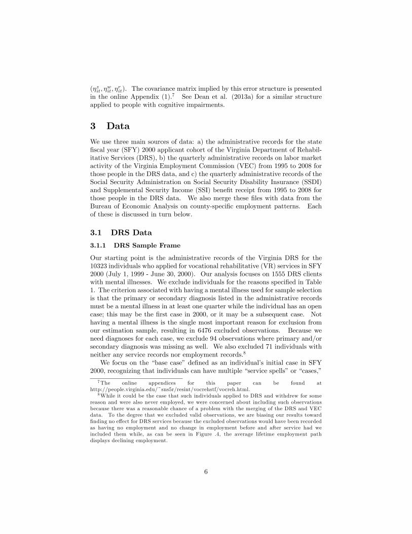
Diagnostic and evaluation services are purchased in 54.7% of the base cases.Purchased services are provided in less than 40% of the cases for every otherservice type. This should be qualified by noting that 16% of applicants arenot accepted into the program, and another 30% drop out after acceptancebut before receiving substantive services. Of the remaining applicants, 80% areprovided a purchased service other than for diagnosis & evaluation. The secondcolumn of Table 2 provides information on the proportion of individuals whoreceive non-purchased services. With the exception of diagnostic & evaluation,the frequency of the receipt of nonpurchased services is very small.A high proportion of clients receive multiple services during the same service

spell. For example, while the most common service combination in the initialservice spell is diagnosis & evaluation with no other service (d), the next mostcommon is diagnosis & evaluation along with restoration (dr), and diagnosis

11 If a particular service type is in both sources, we report the individual as receiving theservice only once.12For example, for diagnosis & evaluation, 6% of the sample had some evidence of receipt

of a nonpurchased service while having no evidence of receipt of a purchased service.13The RSA-911 classifies service receipt into 22 categories. Eighteen of these categories

either map uniquely into DTERMO or have no services reported for this cohort. The remainingfour RSA categories include multiple DTERMO categories. For example, the RSA categorydiagnostic and treatment (D&T) includes both the diagnosis & evaluation category and therestoration category. Using D&T as an example, 6 of the 75 DRS purchased service (PS)categories map into diagnosis & evaluation, and 14 map into restoration. For the individualsflagged by RSA codes as having received D&T, we count the number who received a servicein one or more of the 6 PS codes (call this number, D) and the number in one or moreof the 14 restoration codes (call this number, R). We then assign a probability that anindividual designated in the RSA-911 file as receiving D&T receives diagnosis & evaluationas 0.55 = D/(D +R) and restoration as 0.45 = R/(D +R).

9

NonpurchasedServices Only

Total w/ PositiveExpenditures

w/ ZeroExpenditures

w/ PositiveProbabilities

Diagnosis & Evaluation 0.547 0.477 0.070 0.060Training 0.372 0.362 0.010 0.100Education 0.132 0.131 0.001 0.156Restoration 0.319 0.318 0.001 0.108Maintenance 0.301 0.300 0.001 0.123Other Service 0.234 0.232 0.002 0.140

Table 2: Proportion Receiving DRS Purchased andNonpurchased Service by Type

Service Type

Purchased Services

& evaluation along with training (dt) is the fourth most common. Given thefrequency with which clients receive multiple services, it is critical for us toallow for the possibility of receipt of multiple services. Thus, the structureof the service choice in equation (1) is multivariate discrete choice rather thanpolychotomous discrete choice.Throughout much of the analysis, we measure labor market outcomes relative

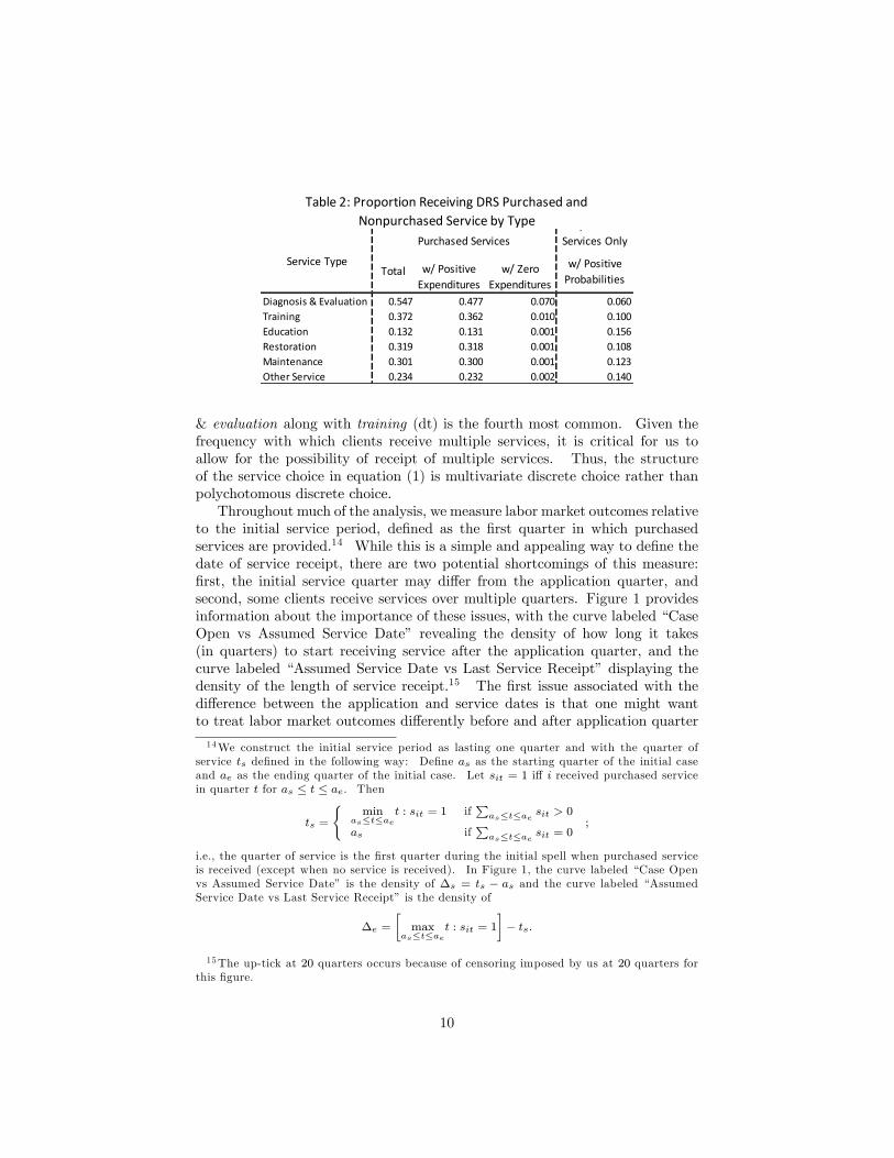
to the initial service period, defined as the first quarter in which purchasedservices are provided.14 While this is a simple and appealing way to define thedate of service receipt, there are two potential shortcomings of this measure:first, the initial service quarter may differ from the application quarter, andsecond, some clients receive services over multiple quarters. Figure 1 providesinformation about the importance of these issues, with the curve labeled “CaseOpen vs Assumed Service Date” revealing the density of how long it takes(in quarters) to start receiving service after the application quarter, and thecurve labeled “Assumed Service Date vs Last Service Receipt” displaying thedensity of the length of service receipt.15 The first issue associated with thedifference between the application and service dates is that one might wantto treat labor market outcomes differently before and after application quarter

14We construct the initial service period as lasting one quarter and with the quarter ofservice ts defined in the following way: Define as as the starting quarter of the initial caseand ae as the ending quarter of the initial case. Let sit = 1 iff i received purchased servicein quarter t for as ≤ t ≤ ae. Then

ts =

min

as≤t≤aet : sit = 1 if

∑as≤t≤ae sit > 0

as if∑as≤t≤ae sit = 0

;

i.e., the quarter of service is the first quarter during the initial spell when purchased serviceis received (except when no service is received). In Figure 1, the curve labeled “Case Openvs Assumed Service Date” is the density of ∆s = ts − as and the curve labeled “AssumedService Date vs Last Service Receipt” is the density of

∆e =

[max

as≤t≤aet : sit = 1

]− ts.

15The up-tick at 20 quarters occurs because of censoring imposed by us at 20 quarters forthis figure.

10

00.05

0.10.15

0.20.25

0.30.35

0.4

0 5 10 15 20 25Difference in Quarters

Density of Differences BetweenRelevant Service Spell Quarters

Case Open vsAssumed ServiceDate

Assumed ServiceDate vs Last ServiceReceipt

Figure 1: Density of Differences Between Relevant Service Spell Quarters

(e.g., the Ashenfelter dip). Instead, we focus on a one-quarter pre-service dip inour specification of the model (see Section 2).The figure shows that 44% startreceiving services in the application quarter and 83% start within 2 quarters.Meanwhile, 3% of DRS clients receive initial services 12 or more quarters afterthe application date. Thus, this issue may not matter that much given theconcentration near zero. The second issue associated with the length of spellsis that there may be a significant difference in labor market outcomes whileservice is being received and after it is finished. In our specification of themodel, we distinguish between outcomes 8 or fewer quarters after service and 9or more quarters after service. Figure 1 shows that 56.1% receive services for 3quarters or less and only 19.1% of applicants are still receiving service after 8quarters. Thus, for the most part, one can interpret the results for 9 or morequarters as being post-service receipt.16

3.1.3 DRS Data for Explanatory Variables

Table 3 provides the sample moments for the explanatory variables comingfrom the DRS data to be used in the analysis. While many of the variablesare standard for this type of analysis, some are unusual and included becauseof the nature of the people being considered. Special education is a dummyvariable equal to 1 for those observations where the respondent received sometype of special education; 2.5% of the respondents received such education.Education information is missing for 10.3% of the sample. Rather than exclude

16One alternative way to define post-service outcomes would be to use the closing date ofthe service spell as the end of service. This is the case for most of the literature (e.g., Deanand Dolan, 1991). The problem with this approach is that counselors do not close casesnecessarily when service provision ends. Another way is to model the transition associatedwith the end of purchased service receipt. We think this is an important long-term researchgoal but beyond the goals of this paper. Alternatively, one could just use the end of servicereceipt as the quarter defining the beginning of relevant labor market outcomes; we weresomewhat concerned with endogeneity issues associated with the length of service receipt andlater labor market outcomes. While our approach has issues associated with it as well, itssimplicity makes it a good place to start exploration of the data.

11

such observations, instead we included a dummy variable for when educationinformation was missing.There are a number of indicators of physical and mental disabilities in the

DRS data. We use four dummy variables, each equal to one if the individual’sprimary or secondary disability at intake in the base SFY 2000 case was diag-nosed as a musculoskeletal impairment, a learning disability, a mental illness,and a substance abuse problem.17 The meaning of mental illness as an ex-planatory variable is that, at the time of application to DRS, the individual’sprimary or secondary diagnosis was mental illness.18 An individual’s coun-selor also assesses the significance of the disability. Three levels are identified:not significant (used as the base level), significant, and most significant. Wealso constructed a dummy for serious mental illness (SMI) based on detaileddiagnostic codes.19

While some variables such as married and # dependents may be endogenous,we follow the literature (e.g., Keith, Regier, and Rae, 1991; Ettner, Frank, andKessler, 1997) and include them anyway as significant indicators of inclusionin society and responsibility. We include a dummy for receipt of governmentfinancial assistance even though it may be endogenous. However, for this pop-ulation, one can work without losing one’s government assistance or having itreduced up to relatively high earnings thresholds. Finally, we include two trans-portation variables: transportation available and has driver’s license. Raphaeland Rice (2002) worries about the endogeneity of these variables and finds thatcontrolling for endogeneity with some reasonable instruments has little effect onthe estimated effect of transportation on employment but makes its effect onwages disappear.To identify the impact of services on labor market outcomes and DI/SSI

receipt, we exploit two instrumental variables that are correlated with the treat-ment assignment but not included in the labor market equations (2) and (3) orthe DI/SSI receipt equation (4). These instruments are the proportion of otherclients in our cohort for the individual’s counselor receiving a particular serviceand the proportion of other clients in our cohort for the individual’s field offi cereceiving a particular service. These variables are transformed as is describedin the online Appendix (2).The properties of these instruments depend upon the distribution of client

size in our sample across counselors and field offi ces20 and the distribution of

17The existence of visual, hearing/speech, internal disabilities, and other miscellaneous dis-abilities and cognitive impairments were available in the data but not common enough or notvarying enough with dependent variables to measure precise effects. So they were not usedin the analysis.18Those in the sample with this explanatory variable equal to zero have a primary or

secondary diagnosis of mental illness at some other point of re-entry into the DRS system inthe future.19Sometimes, SMI is defined in terms of the loss of functionality caused by mental health

problems (U.S. Dept. HHS, 1999). Our data do not provide us with enough information toconstruct such a measure. Instead, we just take the two mental health diagnoses, schizophre-nia and psychosis, among those we observe and define them, for this paper, as having SMI.It is essentially a parsimonious way to aggregate more specific mental health diagnoses.20For example, if most counselors and/or field offi ces had only one client, then this method-

12

Variable Mean Std Dev Variable Mean Std DevMale 0.404 0.491 TypeWhite 0.710 0.454 Musculoskeletal Disability 0.170 0.376Education 10.718 4.931 Learning Disability 0.046 0.209Special Education 0.025 0.156 Mental Illness 0.950 0.218Education Missing 0.103 0.304 Substance Abuse Problem 0.151 0.358Age (Quarters/100) 1.427 0.407Married 0.178 0.383 Extent# Dependents 0.804 1.171 Significant 0.619 0.486Transportation Available 0.741 0.438 Most Significant 0.275 0.446Has Driving License 0.678 0.467 SMI 0.236 0.425Receives Govt Assistance 0.191 0.300

Table 3: Moments of Explanatory VariablesSocio­Demographic Variables Disability Variables

the proportion of clients receiving each service. Figures 2 and 3 provide someinformation about these distributions. In Figure 2, we see that there is signifi-cant variation in the size of counselor caseloads and field offi ce caseloads. Forexample, 43% of counselors have caseloads from our cohort of 5 or less, and7.3% have caseloads of 20 or more. Analogously, 36.7% of field offi ces havecaseloads from our cohort of 10 or less, and 20.5% have caseloads of 50 or more.

Figure 3 shows the empirical distribution of proportion of clients for eachfield offi ce receiving each service. For example, for diagnosis & evaluation,10.4% provide the service to 18.2% of their clients or less, and 4.2% provide itfor all of their clients. Figure 3 shows that diagnosis & evaluation is the mostcommonly provided service, followed by training, then restoration and mainte-nance, then other services, and then education. In fact, except for restorationand maintenance and some choices at very low levels of provision, each curvestochastically dominates the ones behind it across offi ces. The distributions forcounselors have similar properties.There is strong evidence of important variation in behavior across counselors

and across field offi ces.21 We reject the null hypothesis that the joint densityof services within offi ces does not vary across offi ces using a likelihood ratiotest. The test statistic is 407.44 (with 245 df and normalized value of 7.33).We also can test the null hypothesis that each offi ce provides each service inthe same proportion, one at a time, using a likelihood ratio test. The teststatistic is 575.39 (with 294 df and a normalized value of 11.60). For counselors,the analogous test statistics are 970.60 (with 785 df and a normalized value of4.68) and 3836.94 (with 942 df and a normalized value of 66.70). The factthat there is significant variation in the provision of services across offi ces andcounselors make our instrument viable. Whether these instruments satisfy otheridentification restrictions is evaluated in Section 4.2.

ology would not be useful.21While there is significant positive correlation across counselor and offi ce effects, there is

enough independent variation between them to accurately estimate their effects on serviceprovision.

13

0

0.1

0.2

0.3

0.4

0.5

0.6

0.7

0.8

0.9

1

0 20 40 60 80 100 120 140

# Cases

Distribution of # Cases/Office and # Cases/Counselor

# Cases/Office

# Cases/Counselor

Figure 2: Distribution of # Cases/Offi ce and # Cases/Counselor

0.0

0.2

0.4

0.6

0.8

1.0

0.0 0.2 0.4 0.6 0.8 1.0Proportion

Distribution of Proportions Receiving Different Services by Office

Diagnosis & Evaluation

Training

Education

Restoration

Maintenance

Other Services

Figure 3: Distribution of Proportions Receiving Different Services by Offi ce

3.2 VEC Data

One of the unique and valuable features of this analysis is that we have infor-mation from an administrative data source about individual quarterly earningsprior to, during, and after service receipt. Earlier economic analyses of VReffi cacy (Conley, 1969; Bellante, 1972; Worrall, 1978; Nowak, 1983) relied al-most exclusively on the RSA-911 Case Service Report of nationwide closuresfrom the VR program. At the time, the 911 form reported earnings only attwo points: 1) self-reported weekly earnings at the time of referral to the VRprogram and 2) following two months of employment. The latter figure is avail-able only for that portion of VR cases closed “with an employment outcome.”More recent analyses, published almost entirely in the rehabilitation literature(e.g., Cimera, 2010), utilize the same RSA-911 earnings measure, albeit nowcollected after three months of employment. In contrast, this study uses datagleaned from quarterly employment records provided by employers to the Vir-ginia Employment Commission (VEC) for purposes of determining eligibilityfor unemployment insurance benefits.The DRS provided the VEC with identifiers from the universe of 10323 appli-

cants for DRS services in SFY 2000. The VEC returned to DRS a longitudinalfile containing employment data for 9041 individuals having at least one quar-ter of “covered”employment during the 47-quarter period spanning July 1995through March 2009, a “hit rate” of 88%. The remaining 12% in this cohortwere either a) unemployed or out of the labor force for this entire interval orb) employed in jobs that are not covered by the VEC (e.g., were self-employed

14

2001 2002Neither SSA nor VEC show earnings 31% 35%SSA shows earnings, VEC does not 12% 12%VEC shows earnings, SSA does not 1% 1%Both SSA & VEC show earnings 57% 52%

Mean SSA Earnings $9,117 $9,859Mean SSA ­ VEC Difference $510 $616

Table 4: Comparison between SSA and VECEmployment Records

or worked out of state, for federal employers, for very small-sized firms, or atcontingent-type jobs that do not provide benefits).We explored the coverage issue through an arrangement with the Social Se-

curity Administration (SSA) whereby they matched VEC earnings (aggregatedto a calendar year) to calendar-year SSA earnings for all SFY 2000 applicants.22

Table 4 summarizes these results for the 9913 individuals with an identificationmatch. For the two calendar years following SFY 2000 (the fiscal year of appli-cation), the SSA and VEC agreed on employment status for 87% of individuals.VEC records missed employment covered by SSA for 12% of the individuals inboth 2001 and 2002. For those individuals where both SSA and VEC reportearnings, VEC earnings levels fall short of SSA levels by 5.6% in 2001 and 6.2%in 2002.23 Although formally accounting for these coverage errors is beyond thescope of this paper, the results in Table 4 suggests that any resulting biasesshould be minimal for the earnings equations but may be more important forthe employment regressions. Unfortunately, our agreement with the SSA didnot allow us to assess whether these errors varied by VR service receipt. If theerrors are exogenous, the resulting estimates will be consistent. Otherwise, theextent of the bias in non-linear models is diffi cult to assess, especially when theerrors are systematic.Employers report aggregate earnings in a given quarter to the VEC. Re-

call that equations (2) and (3) model employment and earnings impacts in fourseparate periods offset from the date of first service. Because the date of first

22This analysis was not limited to applicants with mental illness diagnoses.23Data from the National Health Interview Survey 2004 Adult Sample (NHIS) show that,

for the United States as a whole, people with mental illness have probabilities of working forthe federal government and being self-employed of 2.7% and 7.8%, respectively; correspondingnumbers for those without mental illness are 3.0% and 8.4%, respectively. However, becauseof its proximity to Washington, DC and its large number of military facilities, Virginia hasan unusually high proportion of federal workers; using data from the Bureau of EconomicAnalysis (2010b), the proportion of employed individuals in Virginia working for the federalgovernment (including the military) in 2000 was 7.6%, while the NHIS data implies that itwas 3.3% for the United States in 2004. If we conclude that 7.8% + (7.6/3.3) ∗ 2.7% = 14.2%of Virginians with mental illness either work for the federal government or are self-employed,this accounts for all of the discrepancy between SSA earnings and VEC earnings in the 2ndrow of Table 4.

15

Before Initial Service Quarter After Initial Service QuarterVariable # Obs Mean Std Dev # Obs Mean Std DevEmployment 31427 0.35 0.477 58763 0.275 0.446Log Quarterly Earnings 11003 7.082 1.492 16145 7.519 1.398

Table 5: Moments of Employment and Earnings Variables

0

0.1

0.2

0.3

0.4

0.5

0.6

­16 ­12 ­8 ­4 0 4 8 12 16 20 24 28 32 36

Rate

Quarter Relative to Date of Application

Employment Rates

Not Treated

Treated

Figure 4: Employment Rates

service can fall anywhere within a quarter, that quarter is excluded from theanalysis other than for use as a period of demarcation separating pre-servicefrom post-service periods. Depending upon the date of first service, this align-ment procedure results in 16 to 19 quarters of pre-service earnings periods and28 to 31 quarters post-service quarters for individuals in this cohort.In our analysis, we try to explain two labor market outcome variables: em-

ployment and log quarterly earnings. Employment is a binary measure of work-ing in a particular quarter in the labor market and is modeled in equation (2).We also measure log quarterly earnings in equation (3). While it would bevaluable to be able to decompose quarterly earnings into wage level and hours,this is not possible in the VEC data. Table 5 provides information on samplesizes and on the moments of employment data and earnings data disaggregatedbetween quarters before and after initial service provision. The sample sizes arequite large and allow us to estimate labor market outcome effects with high pre-cision. One can see that employment rates decline after service provision andquarterly earnings increase (conditional on working). However, as is shownin Section 5, these aggregate facts hide what is really happening and how itdepends on service receipt.Figures 4 and 5 display quarterly employment rates and earnings (conditional

on employment), respectively, for SFY 2000 applicants who receive substantiveVR services and those that do not receive substantial services. We refer tothese two groups as the treated and untreated, respectively. In these figures,quarters are measured relative to application date (not the initial service date)so that quarter 0 is the quarter of application, quarter −4 is one year prior toapplication, and quarter 4 is one year post-application.Perhaps the most striking finding is seen in Figure 4 which shows that, prior

to the application quarter, the employment rates of the treated and untreated

16

0

1000

2000

3000

4000

5000

6000

7000

­16 ­12 ­8 ­4 0 4 8 12 16 20 24 28 32 36

AverageQtrlyEarnings

Quarter Relative to Date of Application

Average Quarterly Earningsfor the Employed

Not Treated

Treated

Figure 5: Average Quarterly Earnings for the Employed

are nearly identical, with a modest Ashenfelter dip in the pre-application quar-ter, but, just after the application quarter, the treated experience a pronouncedincrease in employment rates. For example, one year prior to the applicationquarter, the employment rates are 0.42 for both the untreated and treated,while, one year after the application, the analogous employment rates are 0.35for the untreated and 0.46 for the treated. About one year after the application,the employment rates for both the treated and untreated start to decline, buta gap continues between the two groups. After nine years, the employmentrates of around 0.20 are notably less than the rates in SFY 2000. The observedpost-application increase in employment rates for treated clients may be due toVR services, but it may also reflect endogenous factors. This selection problemwill be addressed using the structural model developed in Section 2.While there is notable association between DRS services receipt and em-

ployment, there is no such relationship with earnings. Figure 5 shows thatquarterly earnings among the employed are almost identical for the treated andthe untreated throughout. Thus, the data reveal that VR treatment servicesare associated with a sharp, substantial, and sustained increase in employmentbut no discernible change in quarterly earnings among the employed.Figures 4 and 5 also shed some light on the appropriate assumption about

the length of the Ashenfelter dip. Depending on the program being evaluated,the pre-program dip in employment and earnings has been generally found tostart between one quarter and one year prior to participation in the program(Heckman et al., 1999; Mueser et al., 2007). For our sample, Figures 4 and5 reveal a dip in earnings in the first quarter prior to the initial service re-ceipt. Thus, we account for the Ashenfelter dip using a one quarter pre-serviceindicator in employment and earnings equations.

3.3 SSA Data

A Memorandum of Agreement (MOA) between the Social Security Adminis-tration (SSA) and the Virginia Department of Rehabilitative Services (DRS)allowed us to obtain monthly SSI (Supplemental Security Income) and DI (Dis-ability Insurance) payments for individuals in our cohort over the period of our

17

analysis. We aggregate SSI and SSDI benefit recipiency into a single binary in-dicator of receipt of disability benefits from either source. We do this becausethe criterion for determining which of the two one receives is about prior accu-mulation of social security benefits, and, for this paper, that is a second-orderissue. In our sample, we observe receipt of disability benefits in 38.4% of theperson/quarters. The correlation of disability benefit receipt and work activity(measured as a binary variable) is −0.293, and the person-specific correlation is−0.189.

3.4 BEA Data

Labor market outcomes may be influenced by local labor market conditions.Though there are no measures of local labor market conditions in either theDRS data or the VEC data, the DRS data contain geographic identifiers sothat we can match each DRS client with their county of residence. The Bureauof Economic Analysis (BEA) provides information on population size and num-ber of people employed, disaggregated by age and county (BEA, 2010a). Weconstruct measures of log employment rates using county level data. Detailsare included in the online Appendix (3).

4 Econometric Methodology

4.1 Likelihood Function

The parameters of the model are θ = (θy, θz, θw, θr,Ωζ) where

θy =(βj , λ

yj1, λ

yj2

)Jj=1

,

θz =(γ, λz1, λ

z2, ρ

zη,[αzjk]Jj=1

),

θw =(δ, λw1 , λ

w2 , ρ

wη , σ

2w,[αwjk]Jj=1

), and

θr =(ψ, λr1, λ

r2, ρ

rη,[αrjk]Jj=1

).

We estimate the parameters of the model using maximum simulated likelihood(MSL). The likelihood contribution for observation i is

Li =

∫Li (ui) dG (ui | Ω) (6)

where

Li (ui) = Lyi (uyi )

T∏t=1

Lzwrit (uzit, uwit, u

rit) ,

Lyi (uyi ) =

J∏j=1

expXyi βj + uyij

1 + exp

Xyi βj + uyij

, (7)

18

Lzwrit (uzit, uwit, u

rit) =

[L0it (uzit, u

wit)]1−zit [

L1it (uzit, uwit)]zit

L2it (urit) , (8)

L0it (uzit, uwit) = 1− Φ

Xzitγ +

K∑k=1

dik

J∑j=1

αzjkyij + uzijt

, (9)

L1it (uzit, uwit) =

1

σwφ

(wit −Xw

it δ −∑Kk=1 dik

∑Jj=1 α

wjkyij − uwit

σw

)· (10)

Φ

Xzitγ +

K∑k=1

dik

J∑j=1

αzjkyij + uzijt

,

L2it (urit) = Φ

Xritψ +

K∑k=1

dik

J∑j=1

αrjkyij + urijt

rit

· (11)

1− Φ

Xritψ +

K∑k=1

dik

J∑j=1

αrjkyij + urijt

1−rit ,and G (ui | Ω) is the joint normal density with covariance matrix Ω describedin the online Appendix (1). While, in general, it is diffi cult to evaluate themultivariate integral in equation (6), it is straightforward to simulate the in-tegral using well-known methods described in Stern (1997). The functionalform of the conditional likelihood contribution associated with observed pro-gram choices, Lyi (uyi ) in equation (7), follows from the assumption in equation(1) that the idiosyncratic errors are iid logit. The functional form of the con-ditional likelihood contribution for labor market outcomes and DI/SSI receipt,Lzwrit (uzit, u

wit, u

rit) in equations (8), (9), (10), and (11) follow from the normal-

ity assumption for (υzit, υwit, υ

rit) and the trivariate normality assumption for

(ζzit, ζwit, ζ

rit) in equation (5). The log likelihood function is

L =

n∑i=1

logLi.

In theory, the parameter estimates are consistent only as the number of inde-pendent draws used to simulate the likelihood contributions goes off to infinity.However, Börsch-Supan and Hajivassiliou (1992) shows that MSL estimates per-form well for small and moderate numbers of draws as long as good simulationmethods are used,24 and Geweke (1988) shows that the simulation error occur-ring in simulation-based estimators is of order (1/n) when antithetic accelerationis used.24We simulate all errors except for η and ε with antithetic acceleration (Geweke, 1988) and

then compute likelihood contributions condition on the simulated errors. This is similar tosimulation methods described in Stern (1992) and McFadden and Train (2000).

19

4.2 Identification

There are two relevant notions of identification in this model. First, there is thegeneral question of identification of model parameters in any nonlinear model.Second, service receipt, labor market outcome variables, and DI/SSI receipt arelikely to be endogenous. With respect to the first issue, covariation in the databetween dependent variables and explanatory variables identifies many of themodel parameters. For example, covariation between male and participationin training identifies the βj coeffi cient in equation (1) associated with the malefor j = training. Similarly, the covariation between white and employmentstatus identifies the γ coeffi cient in equation (2) associated with white, and thecovariation between white and log quarterly earnings identifies the δ coeffi cientin equation (3) associated with white. Similar sample covariances identify para-meters for DI/SSI recipiency in equation (4). Second moment parameters suchas Ωζ in equation (5) are identified by corresponding second sample moments.Two approaches are used to address the second identification problem. First,

as in a difference-in-difference design, we control for pre-treatment labor marketdifferences and DI/SSI receipt between those who do and do not receive services.If the differences in unobserved factors that confound inference in equations (2),(3) and (4), uit, are fixed over time, then controls for the observed pre-treatmentlabor market differences and DI/SSI receipt address the endogenous selectionproblem (see Meyer, 1995; Heckman, LaLonde, and Smith, 1999, Section 4).Second, we include two instruments in equation (1) that are excluded from

equations (2), (3) and (4). As described in Sections 3.1.3 and the online Appen-dix (2), our choice of instruments for service j is the propensity of an individual’scounselor to assign other clients to service j and the propensity of an individual’sfield offi ce to assign other clients to service j.25 Excluding these instrumentsfrom the labor market and DI/SSI equations seems sensible, and, as illustratedin Section 3.1.3, they are strongly correlated with service receipt. However,for these variables to be valid instruments it must also be the case that theyare exogenous. While one can never be certain this holds, there are good rea-sons to think it is a reasonable assumption especially given that we conditionthe analysis on the client’s observed limitations and county level unemploymentrates. Most notably, DRS clients have limited ability to select their field offi ce orcounselor; the field offi ce is determined by the residential location of the client,and, conditional on observed limitations, counselors are randomly assigned.26

So, unless clients relocate to take advantage of the practices of particular fieldoffi ces, the assignment to offi ces and counselors is effectively random conditionalon the observed limitations of clients. A threat to the validity of these instru-ments may arise if variation in the availability of jobs where training (or otherDRS services) is productive might jointly affect labor market outcomes and the

25Doyle (2007), Arrighi et al. (2010), Clapp et al. (2010), Maestas, Mullen, and Strand(2012), and Dean et al. (2013a, 2013b) and use a similar instrument in other applications.26Counselors are assigned by offi ce policy that does not involve client choice. For example,

some field offi ces assign counselors to balance caseload across counselors, some have counselorswho specialize in mental illness, and some assign counselors by client locale.

20

average behavior of counselors and field offi ces. Including measures of local la-bor market conditions directly in equations (2) and (3) should address this issue.A final concern arises if there is significant unobserved variation in the abilityof counselors to match clients with jobs, thus affecting both his/her decisionsabout what type service to offer clients and later success in the labor market.We assume that these types of effects are not important in our analysis.Importantly, our approach for addressing the endogenous selection of ser-

vices represents a substantial advance over the existing literature where thepast research (often using RSA-911 data) generally relies on limited controls forpre-program earnings and assumes service participation is otherwise exogenous.Along with Aakvik, Heckman, and Vytlacil (2005) and Dean et al. (2013a,2013b), this is the first study to identify the impact of VR services on labormarket outcome using both a history of pre-program earnings and plausiblyexogenous instrumental variables.

5 Estimation Results

5.1 Estimates of Impact of VR Services

We divide up the discussion of parameter estimates into separate components.We begin by examining the estimated effect of services on labor market out-comes. Table 6 presents the estimates and associated standard errors for theeffect of services on employment, and Table 7 presents the analogous results forlog quarterly earnings. For each labor market outcome, the effects are allowedto vary across the six different service types and across different time periodsrelative to the initial service quarter. Given our rich labor market data, weare able to estimate both short-run (the first two years) and long-run (morethan two years) effects of services and account for pre-service outcomes in thequarter prior to services as well as two or more quarters prior to the initialservice. As noted in Section 4.2, inclusion of pre-treatment periods is a wayto account for the effect of endogenous selection into services. This method ofcontrolling for selection, which is the central idea of the difference-in-differencedesign, is used extensively in the literature (e.g., Meyer, 1995; Heckman et al.,1999). The quarter immediately prior to initial service provision is separatedout because this quarter seems likely to have a distinct impact on selection andbecause of the well-documented variation in labor market behaviors just priorto the application period —the Ashenfelter dip (Ashenfelter, 1978; Heckman etal., 1999).The first two columns of Tables 6 and 7, which display estimates for the

quarters prior to the initial service, reveal evidence that selection is endoge-nous. Nearly all of the coeffi cients associated with periods two or more quartersprior to the initial service are substantial and statistically different than zero, theone exception being the coeffi cient on restoration in the log quarterly earningsequation. For training and maintenance, the estimates reveal that those peoplewith mental illness provided training services have lower pre-treatment employ-

21

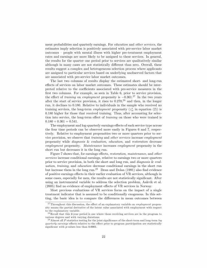
ment probabilities and quarterly earnings. For education and other services, theestimates imply selection is positively associated with pre-service labor marketoutcomes —people with mental illness with higher pre-treatment employmentrates and earnings are more likely to be assigned to these services. In general,the results for the quarter one period prior to services are qualitatively similaralthough in many cases are not statistically different than zero. Overall, theseresults suggest a complex and heterogeneous selection process where applicantsare assigned to particular services based on underlying unobserved factors thatare associated with pre-service labor market outcomes.The last two columns of results display the estimated short- and long-run

effects of services on labor market outcomes. These estimates should be inter-preted relative to the coeffi cients associated with pre-service measures in thefirst two columns. For example, as seen in Table 6, prior to service provision,the effect of training on employment propensity is −0.361.27 In the two yearsafter the start of service provision, it rises to 0.270,28 and then, in the longerrun, it declines to 0.180. Relative to individuals in the sample who received notraining services, the long-term employment propensity (z∗it in equation (2)) is0.180 higher for those that received training. Thus, after accounting for selec-tion into service, the long-term effect of training on those who were trained is0.180 + 0.361 = 0.541.The employment and log-quarterly earnings effects of each service type across

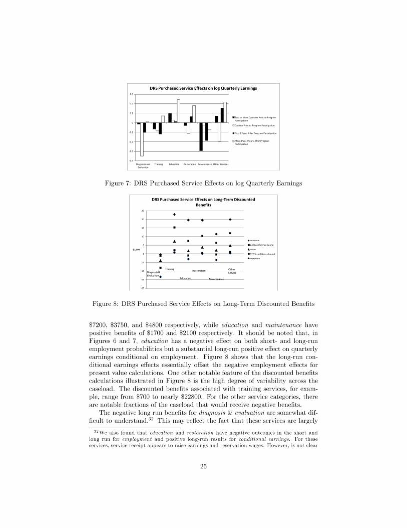
the four time periods can be observed more easily in Figures 6 and 7, respec-tively. Relative to employment propensities two or more quarters prior to ser-vice provision, we observe that training and other services increase employmentpropensity while diagnosis & evaluation, education, and restoration decreaseemployment propensity. Maintenance increases employment propensity in theshort run but decreases it in the long run.Figure 7 shows that, for earnings effects, restoration, maintenance, and other

services increase conditional earnings, relative to earnings two or more quartersprior to service provision, in both the short and long run, and diagnosis & eval-uation, training, and education decrease conditional earnings in the short runbut increase them in the long run.29 Dean and Dolan (1991) also find evidenceof positive earnings effects in their earlier evaluation of VR services, although insome cases, especially for men, the results are not statistically significant. Afterusing an instrumental variable to address the selection problem, Aakvik et al.(2005) find no evidence of employment effects of VR services in Norway.Most previous evaluations of VR services focus on the impact of a single

treatment indicator that is assumed to be conditionally exogenous. In this set-ting, the basic idea is to compare the differences in mean outcomes between

27Throughout this discussion, the effect of an explanatory variable on employment propen-sity means the partial derivative of the latent value associated with employment with respectto the explanatory variable.28Recall that this 2-year period is one where those receiving services are in the program to

various degrees and with varying durations.29Almost all F -statistics testing for the joint significance of the short-term and long-term log

quarterly earnings effects relative to the effect prior to program participation are statisticallysignificant with p-values less than 0.0001.

22

VariableDiagnosis & Evaluation 0.280 ** 0.091 0.052 ** ­0.182 **

(0.008) (0.081) (0.014) (0.007)Training ­0.361 ** ­0.168 * 0.270 ** 0.180 **

(0.010) (0.101) (0.017) (0.008)Education 0.283 ** 0.175 ­0.016 0.170 **

(0.014) (0.134) (0.025) (0.010)Restoration 0.275 ** 0.461 ** 0.258 ** 0.148 **

(0.010) (0.092) (.018) (0.008)Maintenance ­0.217 ** ­0.222 ** ­0.163 ** ­0.291 **

(0.011) (0.113) (0.019) (0.009)Other Services 0.156 ** ­0.035 0.284 ** 0.205 **

(0.011) (0.122) (0.020) (0.009) Notes:

2.Single­starred items are statistically significant at the 10% level, and double­starred items are statistically significant at the 5% level.

Table 6: DRS Purchased Service Participation Effects onEmployment PropensityTwo or More

QuartersPrior toService

Participation

QuarterPrior toService

Participation

First 2 YearsAfter ServiceParticipation

More than 2Years After

ServiceParticipation

1.Standard errors are in parentheses.

­0.5

­0.4

­0.3

­0.2

­0.1

0

0.1

0.2

0.3

0.4

0.5

0.6

Diagnosis andEvaluation

Training Education Restoration Maintenance Other Services

DRS Purchased Service Effects on Employment Propensity

Two or More Quarters Prior to ProgramParticipation

Quarter Prior to Program Participation

First 2 Years After Program Participation

More than 2 Years After Program Participation

Figure 6: DRS Purchased Service Effects on Employment Propensity

23

VariableDiagnosis & Evaluation ­0.017 ** ­0.349 ** ­0.102 ** 0.015

(0.013) (0.107) (0.025) (0.011)Training ­0.065 ** ­0.086 ­0.120 ** 0.071 **

(0.017) (0.159) (0.031) (0.014)Education 0.096 ** 0.027 0.011 0.242 **

(0.022) (0.186) (0.042) (0.017)Restoration ­0.028 * ­0.116 0.064 ** 0.178 **

(0.015) (0.123) (0.031) (0.013)Maintenance ­0.293 ** ­0.027 ­0.187 ** ­0.076 **

(0.018) (0.169) (0.033) (0.013)Other Services 0.070 ** ­0.199 0.154 ** 0.216 **

(0.017) (0.176) (0.032) (0.014) Notes:

2.Standard errors are in parentheses.3.Single­starred items are statistically significant at the 10% level, and double­starred items are statistically significant at the 5% level.

Table 7: DRS Purchased Service Participation Effects on LogQuarterly Earnings

Two or MoreQuartersPrior toService

Participation

QuarterPrior toService

Participation

First 2 YearsAfter

ServiceParticipation

More than 2Years After

ServiceParticipation

1.Estimates are effects on log quarterly earnings conditional on employment.

treatment and control groups after conditioning on observed variables. Forexample, Figures 4 and 5 above, which display the unconditional mean employ-ment and earnings outcomes respectively, reveal little pre-program differences,fairly substantial positive post-treatment employment associations, and almostno relationship between treatment and earnings. The structural model esti-mated in this paper extends this approach in several important ways: first, byconditioning on observed covariates; second, by accounting for six different typesof service rather than a single treatment indicator; and finally, by using instru-mental variables in a model with endogenous service provisions. The resultsfrom the structural model estimates presented in this section suggest a muchmore complex and nuanced story, with evidence of pre- and post-program labormarket differences that vary across services, estimated employment effects thatare positive for some services and negative for others, and estimated earningseffects that are consistently positive in the long run.Because of the variation in effects over time and over labor market out-

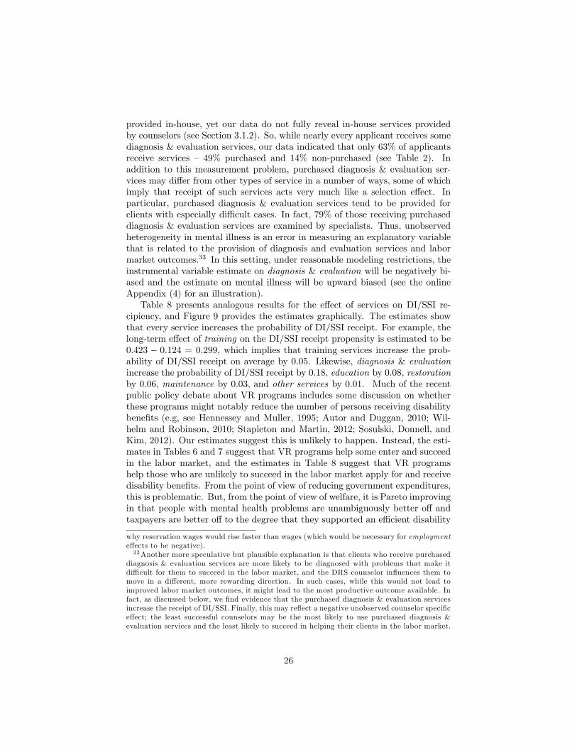
comes seen in Figures 6 and 7, it is diffi cult to infer the long-run benefits ofeach service. Figure 8 reports the mean present value for 10 years of earningsflows (measured in $1000) excluding service costs , a 95% confidence range,30

and the minimum and maximum present value of each service.31 Except fordiagnosis & evaluation, all of the services have positive long-run benefits. Onaverage, training, restoration, and other services have benefits on the order of

30The 95% confidence range provides information about the variation in benefits across in-dividuals caused by the nonlinearity of the model and variation in other explanatory variables.31We use a quarterly discount factor of 0.95. Because the distribution of benefits is highly

skewed, the normal approximation is not appropriate. Instead, we report the 0.025 and 0.975quantiles of the empirical distribution.

24

­0.4

­0.3

­0.2

­0.1

0

0.1

0.2

0.3

Diagnosis andEvaluation

Training Education Restoration Maintenance Other Services

DRS Purchased Service Effects on log Quarterly Earnings

Two or More Quarters Prior to ProgramParticipation

Quarter Prior to Program Participation

First 2 Years After Program Participation

More than 2 Years After ProgramParticipation

Figure 7: DRS Purchased Service Effects on log Quarterly Earnings

­20

­15

­10

­5

0

5

10

15

20

25

$1,000

DRS Purchased Service Effects on Long­Term DiscountedBenefits

minimum

2.5% confidence bound

mean

97.5% confidence bound

maximum

Diagnosis &Evaluation

Training

Education

Restoration

Maintenance

OtherService

Figure 8: DRS Purchased Service Effects on Long-Term Discounted Benefits

$7200, $3750, and $4800 respectively, while education and maintenance havepositive benefits of $1700 and $2100 respectively. It should be noted that, inFigures 6 and 7, education has a negative effect on both short- and long-runemployment probabilities but a substantial long-run positive effect on quarterlyearnings conditional on employment. Figure 8 shows that the long-run con-ditional earnings effects essentially offset the negative employment effects forpresent value calculations. One other notable feature of the discounted benefitscalculations illustrated in Figure 8 is the high degree of variability across thecaseload. The discounted benefits associated with training services, for exam-ple, range from $700 to nearly $22800. For the other service categories, thereare notable fractions of the caseload that would receive negative benefits.The negative long run benefits for diagnosis & evaluation are somewhat dif-

ficult to understand.32 This may reflect the fact that these services are largely

32We also found that education and restoration have negative outcomes in the short andlong run for employment and positive long-run results for conditional earnings. For theseservices, service receipt appears to raise earnings and reservation wages. However, is not clear

25

provided in-house, yet our data do not fully reveal in-house services providedby counselors (see Section 3.1.2). So, while nearly every applicant receives somediagnosis & evaluation services, our data indicated that only 63% of applicantsreceive services — 49% purchased and 14% non-purchased (see Table 2). Inaddition to this measurement problem, purchased diagnosis & evaluation ser-vices may differ from other types of service in a number of ways, some of whichimply that receipt of such services acts very much like a selection effect. Inparticular, purchased diagnosis & evaluation services tend to be provided forclients with especially diffi cult cases. In fact, 79% of those receiving purchaseddiagnosis & evaluation services are examined by specialists. Thus, unobservedheterogeneity in mental illness is an error in measuring an explanatory variablethat is related to the provision of diagnosis and evaluation services and labormarket outcomes.33 In this setting, under reasonable modeling restrictions, theinstrumental variable estimate on diagnosis & evaluation will be negatively bi-ased and the estimate on mental illness will be upward biased (see the onlineAppendix (4) for an illustration).Table 8 presents analogous results for the effect of services on DI/SSI re-

cipiency, and Figure 9 provides the estimates graphically. The estimates showthat every service increases the probability of DI/SSI receipt. For example, thelong-term effect of training on the DI/SSI receipt propensity is estimated to be0.423 − 0.124 = 0.299, which implies that training services increase the prob-ability of DI/SSI receipt on average by 0.05. Likewise, diagnosis & evaluationincrease the probability of DI/SSI receipt by 0.18, education by 0.08, restorationby 0.06, maintenance by 0.03, and other services by 0.01. Much of the recentpublic policy debate about VR programs includes some discussion on whetherthese programs might notably reduce the number of persons receiving disabilitybenefits (e.g, see Hennessey and Muller, 1995; Autor and Duggan, 2010; Wil-helm and Robinson, 2010; Stapleton and Martin, 2012; Sosulski, Donnell, andKim, 2012). Our estimates suggest this is unlikely to happen. Instead, the esti-mates in Tables 6 and 7 suggest that VR programs help some enter and succeedin the labor market, and the estimates in Table 8 suggest that VR programshelp those who are unlikely to succeed in the labor market apply for and receivedisability benefits. From the point of view of reducing government expenditures,this is problematic. But, from the point of view of welfare, it is Pareto improvingin that people with mental health problems are unambiguously better off andtaxpayers are better off to the degree that they supported an effi cient disability

why reservation wages would rise faster than wages (which would be necessary for employmenteffects to be negative).33Another more speculative but plausible explanation is that clients who receive purchased

diagnosis & evaluation services are more likely to be diagnosed with problems that make itdiffi cult for them to succeed in the labor market, and the DRS counselor influences them tomove in a different, more rewarding direction. In such cases, while this would not lead toimproved labor market outcomes, it might lead to the most productive outcome available. Infact, as discussed below, we find evidence that the purchased diagnosis & evaluation servicesincrease the receipt of DI/SSI. Finally, this may reflect a negative unobserved counselor specificeffect; the least successful counselors may be the most likely to use purchased diagnosis &evaluation services and the least likely to succeed in helping their clients in the labor market.

26

VariableDiagnosis & Evaluation ­0.562 ** ­0.139 0.244 ** 0.667 **

(0.014) (0.151) (0.019) (0.008)Training 0.124 ** 0.574 ** 0.592 ** 0.423 **

(0.015) (0.189) (0.027) (0.009)Education ­0.176 ** 0.383 0.471 ** 0.345 **

(0.026) (0.282) (0.044) (0.013)Restoration ­0.691 ** ­0.779 ** ­0.699 ** ­0.161 **

(0.019) (0.236) (0.025) (0.009)Maintenance ­0.179 ** ­0.009 0.193 ** 0.054 **

(0.016) (0.202) (0.028) (0.010)Other Services ­0.545 ** ­0.318 ­0.366 ** ­0.391 **

(0.018) (0.230) (0.031) (0.010) Notes:

2.Standard errors are in parentheses.3.Single­starred items are statistically significant at the 10% level, and double­starred items are statistically significant at the 5% level.

Table 8: DRS Purchased Service Participation Effects on DI/SSIParticipation PropensityTwo or More

QuartersPrior toService

Participation

QuarterPrior toService

Participation

First 2 YearsAfter

ServiceParticipation

More than 2Years After

ServiceParticipation

1.Estimates are effects on DI/SSI Participation Propensity.

­1

­0.8

­0.6

­0.4

­0.2

0

0.2

0.4

0.6

0.8

Diagnosis andEvaluation

Training Education Restoration Maintenance Other Services

DRS Purchased Service Effects on DI/SSI Propensity

Two or More Quarters Prior to ProgramParticipation

Quarter Prior to Program Participation

First 2 Years After Program Participation

More than 2 Years After ProgramParticipation

Figure 9: DRS Purchased Service Effects on DI/SSI Propensity

benefits program in the first place.

5.2 Estimates of the Impact of Covariates

Estimates of the effects of demographic characteristics on the propensity to usedifferent services (y∗ijt in equation (1)) are provided in the online Appendix (5).For the most part, the observed characteristics do not have statistically signifi-cant effects on service receipt, but there are some interesting exceptions. We findthat clients with learning disabilities (0.680) and those receiving government as-sistance (0.491) are more likely to receive diagnosis & evaluation services. Theprobability of receiving training is higher for persons with government assis-tance (0.777) but lower for men (−0.315) and for those with musculoskeletaldisabilities (−0.489) and/or substance abuse problems (−0.373). The receipt ofeducation increases for those with more education (0.082) and for those with

27

Std ErrCounselor Effect 0.344 ** 0.103Office Effect 0.767 ** 0.069Missing Counselor EffectsDiagnosis & Evaluation ­0.431 0.350Training 0.105 0.421Education ­0.753 * 0.433Restoration ­0.486 0.362Maintenance ­0.360 0.410Other Services ­0.393 0.409 Notes:

Estimate

Table 9: Counselor and Office Effectson Service Receipt

1.Single­starred items are statisticallysignificant at the 10% level, and double­starreditems are statistically significant at the 5% level.2.Other than those reported, missing counselorand field office effects parameters wereexcluded because of multicollinearityproblems.

access to transportation and a driver’s license (0.679). Interestingly, however,there is no statistically significant effect associated with having a serious mentalillness or a significant disability.34

Table 9 presents estimates of counselor and offi ce effects as defined in theonline Appendix (2). There are two types of coeffi cient estimates reported inthe table: a) the counselor and offi ce effects and b) the missing counselor effects.The counselor and offi ce effects should be interpreted as ∂Ey∗ij/∂ei where y

∗ij is

the latent variable associated with receipt of service j in equation (1) and ei isthe counselor or offi ce effect defined in the online Appendix (2); note that theseare restricted to be the same across different services. The missing counseloreffects are the effect on y∗ij when the relevant counselor does not have enoughother clients to compute a set of counselor effects.35 These counselor and offi ceinstrumental variables turn out to have large and statistically significant effectson service provision across clients. One should note that we are controlling for apretty full set of demographic characteristics. So it is unlikely that these resultsreflect variation in the mix of clients across counselors and/or field offi ces.Table 10 reports the effects of the demographic, socioeconomic, and disability-

related characteristics on the three labor market outcomes of interest (z∗it inequation (2), wit in equation (3), and r∗it in equation (4)). For labor marketoutcomes, almost all of the estimates are statistically significant. Many of theestimates are as expected including positive effects of being white on employ-ment propensity (0.157) and log quarterly earnings (0.362) as well as positiveeffects of education on employment propensity (0.024) and log quarterly earn-

34The education missing variable is statistically significantly negative across almost allservices. It turns out that almost all of the individuals with education missing were closedduring the application process. Thus, in an important sense, causation for this variable runsthe other way.35We allow missing counselor effects to vary over services. However, we restrict missing

offi ce effects coeffi cients to be zero because there are not enough cases and those that existare too highly correlated with missing counselor effects to estimate both with any precision.

28

ings (0.053). The two transportation variables also have positive impacts onboth labor market outcomes. The local labor market employment rate increasesemployment probabilities but decreases conditional earnings, suggesting that itmight have been useful to include a measure of local wage rates. Some of the de-mographic and socioeconomic parameter estimates are counterintuitive. In par-ticular, having a serious mental illness (SMI) increases employment propensity(0.194), receipt of special education increases log quarterly earnings (0.259),36

while being married decreases both employment propensity (−0.322) and logquarterly earnings (−0.138). The marriage effects can occur through incomeeffects associated with having a spouse.The diagnosis of a mental illness in the “base case” versus being initially

diagnosed with mental illness in a subsequent application for VR services hasa negative effect on employment propensity (−0.210) while increasing log quar-terly earnings (0.399). Meanwhile, the disability severity-related variables havethe expected signs, with negative effects of significant and most significant dis-abilities (relative to mild) on both labor market outcomes. Unlike its impact onservice provision, the SMI estimates are explaining a significant amount of vari-ation in labor market outcomes. SMI, by itself, increases employment (0.194)and increases log quarterly earnings (0.964). For males and whites, there areadded interaction effects, all adversely affecting labor market outcomes. How-ever, overall, the estimates with respect to SMI effects are hard to explain.Education interacted with SMI has negative effects, and age interacted withSMI has mixed but statistically significant effects on outcomes. Baldwin (2005)estimates the effect of mood disorder, anxiety disorder, and adjustment disor-der on employment probabilities and finds an average reduction in employmentprobability on the order of 0.3 (see McKeithen and Stern, 2007, for calculations).Our estimates imply smaller effects, at least for significant mental health prob-lems similar to those considered by Baldwin. A big part of the reason for thisis probably that our sample consists only of people who have been identified ashaving a mental health problem while Baldwin (2005) uses the SIPP sample.For DI/SSI receipt, almost all of the effects are statistically significant and

with expected signs, also. For example, the probability a client takes-up DI/SSIis estimated to decrease for white (−0.114), education (−0.044), and trans-portation available (−0.068). Surprises are married (0.484), learning disability(−0.166), and local employment rate (0.050).So far all of the discussion has concerned the effect of purchased services on

labor market outcomes. In fact, DRS also provides some services in-house, andother services sometimes are paid for by other organizations, and, as discussedin Section 3.1.2, we have some information about those other services. Usingthis data, we allow the effects of covariates on the receipt of such services to beproportionate to their effect for service choice in equation (1) and their effect foremployment propensity in equation (2) as reported in Table 6, for conditionallog quarterly earnings in equation (3) as reported in Table 7, and for DI/SSI36Special education programs have been found to improve schooling outcomes (Hanushek et

al., 2002) and are associated with the use of supported employment services linked to higherearnings (Drake et al., 2009).

29

Variable Std Err Std Err Std Err

Constant 0.052 ** 0.021 5.311 ** 0.032 ­3.338 ** 0.026Male 0.024 ** 0.006 0.360 ** 0.008 ­0.036 ** 0.007White 0.157 ** 0.007 0.362 ** 0.009 ­0.114 ** 0.009Education 0.024 ** 0.001 0.053 ** 0.001 ­0.044 ** 0.001Special Education ­0.014 0.027 0.259 ** 0.032 ­0.019 0.024Education Missing 0.423 ** 0.013 0.626 ** 0.020 ­0.438 ** 0.015Age/100 ­0.701 ** 0.007 0.043 ** 0.009 1.358 ** 0.010Married ­0.322 ** 0.007 ­0.138 ** 0.009 0.484 ** 0.009# Dependents 0.061 ** 0.002 0.064 ** 0.003 ­0.063 ** 0.003Transportation Available 0.122 ** 0.007 0.089 ** 0.009 ­0.068 ** 0.007Has Driving License 0.213 ** 0.007 0.333 ** 0.010 ­0.175 ** 0.007Receives Govt Assistance ­0.332 ** 0.008 ­0.237 ** 0.012 1.753 ** 0.009Musculoskeletal Disability 0.097 ** 0.007 0.130 ** 0.009 0.036 ** 0.009Learning Disability 0.406 ** 0.012 0.225 ** 0.015 ­0.166 ** 0.015Mental Illness ­0.210 ** 0.012 0.399 ** 0.018 ­0.016 0.013Substance Abuse 0.213 ** 0.007 0.086 ** 0.010 ­0.366 ** 0.009Disability Significant ­0.027 ** 0.009 ­0.170 ** 0.012 0.664 ** 0.011Disability Most Significant ­0.112 ** 0.010 ­0.280 ** 0.013 1.147 ** 0.012SMI 0.194 ** 0.028 0.964 ** 0.038 1.083 ** 0.032Male * SMI ­0.094 ** 0.012 ­0.521 ** 0.017 0.513 ** 0.014White * SMI ­0.535 ** 0.012 ­0.482 ** 0.018 0.815 ** 0.014Education * SMI ­0.019 ** 0.001 ­0.047 ** 0.002 0.044 ** 0.001Age/100 * SMI 0.236 ** 0.015 ­0.083 ** 0.021 ­1.249 ** 0.016Local Employment Rate 0.185 ** 0.067 ­0.185 ** 0.068 0.050 ** 0.011

DI/SSI ReceiptEstimate

Note: Single­starred items are statistically significant at the 10% level, and double­starred items arestatistically significant at the 5% level.

Employment Log Quarterly EarningsEstimate Estimate

Table 10: Labor Market and DI/SSI Effects

receipt in equation (4) as reported in Table 8. The estimated proportion forservice choice propensity is 0.824∗∗ (0.280), and the estimated proportion for theeffect of services on employment propensity, conditional log quarterly earnings,and DI/SSI receipt propensity is 0.432∗∗ (0.033); i.e., decisions about usingnonpurchased services are similar to those for purchased services (because 0.824is not statistically significantly different from 1.0), and the effect on such serviceson labor market outcomes and DI/SSI receipt is 43.2% of that for purchasedservices.

5.3 Estimates of the Covariance Structure

Our model has a rich error covariance structure, as seen in equation (5). Thisallows for the possibility that unobservables associated with service provisionare correlated with unobservables associated with labor market outcomes. Thefactor loadings for Factor 1 in Table 11 demonstrate no statistically significantcorrelations between the errors associated with the provision of all service typesand the error associated with employment propensity. However, the correla-tion between the errors for employment propensity and log quarterly earningsis positive (0.556 and 0.436) and the correlation between the errors for employ-ment and DI/SSI receipt are negative (0.556 and −0.225). This suggests thatthere is some unobserved personal characteristic, maybe ability, that increasesemployment probabilities and conditional earnings but decreases DI/SSI receiptprobabilities.Meanwhile, the factor loadings for Factor 2 imply negative correlation be-

tween the errors associated with log quarterly earnings and DI/SSI receipt

30

Variable Std Err Std ErrDiagnosis & Evaluation ­0.055 0.065 ­0.032 0.069Training 0.006 0.085 ­0.065 0.083Education ­0.064 0.109 ­0.152 0.110Restoration ­0.039 0.075 ­0.143 * 0.083Maintenance ­0.056 0.086 0.197 ** 0.088Other Services 0.022 0.088 ­0.257Employment 0.556 ** 0.003 ­0.002 0.003Log Quarterly Earnings 0.436 ** 0.004 ­0.116 ** 0.004SSI/DI ­0.225 ** 0.003 1.652 ** 0.005 Notes:

2.The identifying condition associated with the factor loadings is thatthe factor loadings for the six different services are orthogonal. Weimpose this condition by computing the factor loading for factor 2 onother services as a function of the other 11 relevant factor loadings. Thefactor loadings associated with labor market outcomes are not part ofthe orthogonality condition.

Table 11: Covariance Factor LoadingsFactor 1 Factor 2

Estimate Estimate

1.Single­starred items are statistically significant at the 10% level, anddouble­starred items are statistically significant at the 5% level.

Variable Std Err Variable Std ErrVar(ζ1) 0.041 ** 0.000 Var(ζ2) 0.008 ** 0.004

Cov(ζ1,ζ2) 0.018 ** 0.005 Cov(ζ2,ζ3) ­0.018 ** 0.005

Cov(ζ1,ζ3) ­0.040 ** 0.000 Var(ζ3) 0.041 ** 0.0000.000 σw 1.281 ** 0.003

Note: Double­starred items are statistically significant at the 5% level.

EstimateTable 12: Other Covariance Terms

Estimate

(−0.116 and 1.652). This suggests another unobserved characteristic, perhapssome other component of ability, increasing log quarterly earnings and decreas-ing DI/SSI receipt but having no real impact on employment propensity. Theestimates of the factor loadings for service provision imply that neither unob-served component has any meaningful effect on service provision except formaintenance which is positively correlated with DI/SSI receipt (0.197 and1.652).The estimates of the other elements of the error structure are reported in Ta-

ble 12. All of the estimated covariance terms are relatively small and dominatedby the factor structure terms in Table 11. The estimate of the log earningserror σw is quite large, implying that a standard deviation in quarterly earningsdue to unobserved factors is on the order of $8546. It is unclear how much ofthis variation is due to variation in wages and how much is due to variation inhours. Baldwin (2005) finds wage effects on the order of −0.2 (see McKeithenand Stern, 2007, for calculations) but does not estimate hours effects.

31

5.4 Specification Tests

We use standard goodness-of-fit tests to measure how well we are predictingservice provision probabilities. For each service, we decompose the sampleinto 40 cells, each of length 0.025, stratified by the predicted probability ofservice receipt.37 Then we construct the standard χ2 test statistic. For serviceprovision probabilities, we fail to reject the null that the model predictions equalobserved probabilities at the 5% percent significant level.We perform the same test for employment probabilities disaggregated into

probabilities before and after service receipt.38 The test statistics are χ231 =288.29 for employment probabilities before service receipt and χ232 = 109.87 foremployment probabilities after service receipt. Both of these are highly signifi-cant implying a poor fit. Figure 10 plots the deviations between predicted andsample employment probabilities for the two periods. Deviations between the45 line and the other two sample lines at any particular predicted probabilityrepresent that part of employment probability that we are not predicting. Themodel does a good job predicting employment probabilities both periods upto a predicted probability of about 0.7, after which the fit worsens. Overall,while we are basically grouping individuals into the correct range of employmentprobabilities, there is some concern that, between 0.2 and 0.5, we are underesti-mating employment probabilities prior to VR service receipt and overestimatingit after VR service receipt; this may have a large effect on our rate-of-returnanalysis later in Section 6.Finally, for DI/SSI receipt, the test statistics are χ235 = 368.8 for DI/SSI

probabilities before service receipt and χ238 = 1218.1 for DI/SSI probabilitiesafter service receipt. However, the curves analogous to Figure 10 look extremelysimilar to those in Figure 10 (once smoothed);39 they fit very well until predictedprobabilities above 0.7 (where there many fewer observations).Also, using a series of Lagrange Multiplier (LM) tests, we consider allowing

for interactions among pairs of services in the labor market outcome equations.While the nonlinearity of the model creates some interactions, it may not beappropriate to rely strictly on the model structure. These LM tests, however,suggests that is not important to allow for service interactions. Similarly, wetest for interactions between demographic characteristics (male and white) andservices, but find no evidence of such interactions.

6 Rate of Return

The preceding analysis suggests that, except for purchased diagnosis & eval-uation services, observed DRS services have long-run positive effects on labormarket outcomes (see Figure 8). In this section, we examine the social welfareimplications of VR services by comparing the estimated benefits and costs of

37For each test, some cells are empty and therefore not used.38Before service receipt includes the quarter before receipt, and after service receipt includes

both quarters in the first two years after receipt and the longer run.39The graph for DI/SSI receipt is available in the online Appendix (6).

32

0

0.1

0.2

0.3

0.4

0.5

0.6

0.7

0.8

0.9

1

0 0.2 0.4 0.6 0.8 1

Sample Probability

Predicted Probability

Predicted and Sample Employment Probabilities

Before

After

45° Line

Figure 10: Predicted and Sample Employment Probabilities

the program. The primary monetary benefits and costs of VR services are es-timated using our model and the DRS data on the costs of purchased services.There are, however, many factors for which we do not have direct evidence onthe associated costs. In particular, the costs of nonpurchased services are notobserved in the DRS data file. For these items, we present more speculativeevidence.We simulate the private labor market benefits to DRS clients using the struc-

tural model estimates summarized in Section 5.40 In particular, we compute themean present discounted value of the provided services relative to the value ofreceiving no services using both a 5- and 10-year post-treatment observationperiod for those individuals who received some service and using an annual dis-count factor of 0.987. The estimated mean discounted benefits are $1942 with astandard deviation of $3726 using the 5-year window and $4124 with a standarddeviation of $7677 using a 10-year window.A more accurate estimate of the mean discounted benefits of VR services

may be found by excluding diagnosis & evaluation services from the benefitscomputation. As noted in Section 5, the estimated long-run benefits associateddiagnosis & evaluation services is likely to be downward biased. While the extentof this bias is unknown, there is no reason to think that these services have anegative effect. Thus, setting the benefits of diagnosis & evaluation to zero will

40This simulation has a similar structure to the one used to compute marginal effects inSection 5.1 (see Figure 8). But here we compute the present discounted value of the ac-tual treatments provided by DRS rather than a conjectured treatment for single service, j.Formally, we first compute the short- and long-run effect of the program for each individual:

∆i = vik (yi)− vik (0)

where vik (yi) is the estimated labor market earnings under the realized services yi and vik (0)is the estimated earnings that would be observed if no services were provided.

33

lead to a conservative and more accurate estimate of the long-run benefits. Inthis scenario, we estimate that the mean discounted benefits are $4233 with astandard deviation of $3678 using the 5-year window and $8374 with a standarddeviation of $7744 using a 10-year window.While these estimated benefits are derived directly from the structural model,

there are several reasons they may not reflect the true social benefits of VRservices. First, some of the estimated earning benefits may reflect the displace-ment of non-VR participants, particularly if VR services do not improve theVR participant skills or the job matching process. In general, however, trainingprograms for low-skilled workers are not thought to cause notable labor marketdisplacements (see Lalonde, 1995). Second, VR services may lead to other so-cial benefits associated with the increased attachment to the labor market andthe resulting reduction in use of the social welfare system. While society doesnot benefit from reduced transfer payments or increased tax revenues —taxpayergains exactly offset VR participant losses (except for changes in deadweight loss)— social benefits may result from reduced administrative cost associated withwelfare programs and increased VR participant utility due to reduced welfaredependence (Lalonde, 1995), improved health status, and access to health careinsurance. At the same time, the deadweight costs of taxations may changeif welfare receipt and tax payments change. . Likewise, we do not include theestimated positive impact of VR services on DI/SSI receipt. Finally, there issubstantial heterogeneity in the discounted benefits across the VR participants,suggesting that there may be a great deal of variation in the overall benefitsestimates (see Figure 8). Many of the clients are estimated to have negativebenefits from VR services.As noted in Section 3, DRS services are provided in any combination of three

ways: a) internally by DRS personnel, b) as a “similar benefit”(i.e., purchasedor provided by another governmental agency or not-for-profit organization withno charge to DRS), and/or c) as a purchased service through an outside vendorusing DRS funds. The DRS data report purchased services but not in-houseservices or “similar benefits.”Table 13 displays the mean costs of purchased ser-vices for each service. Interestingly, the average cost for training is substantiallyless than the mean long-term discounted marginal benefit of $7700 (see Figure8). Overall, the mean costs of purchased services among all 1260 clients whouse purchased services equals $1903 with a standard deviation of $1372. Thesemean cost estimates have not been discounted, and thus will be inflated to theextent the purchased services are provided over long periods.The DRS data do not provide information on the costs other than purchased

services (missing are DRS-provided services, “similar benefits,”and the cost ofadministrating the program). To estimate these costs, we use information onDRS spending by fiscal year as reported to the US Social Security Administra-tion. These reports summarize information on aggregate administrative costs,DRS-provided counseling, guidance, and placement service costs, purchased ser-vice cost, WWRC costs, and size of the caseload for each fiscal year. Exceptfor the WWRC reports, these reports do not provide information on the costs

34

ServiceMean

ExpenditureStd

DeviationDiagnosis & Evaluation $290 $567Training $1,712 $2,946Education $1,538 $2,668Restoration $730 $1,226Maintenance $839 $2,302Other Services $247 $1,123

Table 13: Moments of Expenditure Dataon Purchased Services Conditional on

Positive Expenditure

Note: Moments do not include cost ofnonpurchased services.

associated with “similar benefits.”41 While there is some variation in the distrib-ution of costs across years, in general, non-purchased service and administrativecosts account for 45% of total expenditures, reflecting an average cost per clientof roughly $200 per month.

While these reports do not provide information specific to the different im-pairment groups, this auxiliary information can be used to infer the cost forour sample of applicants with mental illnesses. Two different approaches areused. In the first, we anchor on the fact that purchased services account for55% of total VR costs. Given that purchased service costs for our sample av-erage $1903 per client receiving purchased services, fixed costs are estimatedto be $1560 (≈ ($1903/0.55) − $1903) per client. In the second, we anchor onthe fact that the average costs of administration and non-purchased services is$200 per client-month. Given that the average service spell length is 6 quarters,these costs are estimated to be $3600 (= 3 ∗ 6 ∗ 200) per client. These twoestimates reflect our uncertainty about the costs of non-purchased services andadministration. Cases of individuals with mental illness may differ from thegeneral population in both average purchased service expenditures and averagespell lengths. So, if cases of individuals with mental illness have low averagepurchased services relative to non-purchased service costs, the first approachwould be downward-biased. If instead, such cases have relatively low averagecosts associated with administration or non-purchased services, the second ap-proach would be upward-biased. Finally, note that we do not compute separateestimates based on client-specific information on purchased services and spelllength. We choose to use only an average “fixed”cost because the model and

41The fraction of clients estimated to receive (non-WWRC) similar benefits range frombetween 9% for other services to 16% for education services, but in general these services areprovided in combination with DRS purchased services. The fraction of clients only receivingsimilar benefits varies from 3-4% for diagnosis & evaluation, training, and restoration, to 5-6%for maintenance and other, and to 8% for education.

35

estimation procedure used to infer benefits does not allow actual expendituresto affect labor market outcomes.Comparing these estimated costs and benefits reveals that DRS services

provided to mentally ill people have a substantial positive return especially inthe longer run. In total, our preferred estimates, which exclude diagnosis &evaluation, imply that mean benefits range from $4233 for the short run to$8374 for the long run, while mean costs range from $3200 to $5000. Thus,even under the most conservative assumptions about the costs of services, thelong-run social benefit is estimated to exceed costs by 67%.

We also can compute the rate of return for each person receiving servicesin our sample. The results of this exercise are reported in Figure 11. Foreach sample individual receiving some service, we compare the expected flow ofbenefits they would get with the service package they received relative to theflow of benefits they would get with no services. We approximate cost as42

f +

J∑j=1

yijcj

where f is a combination of administrative costs and average (unobserved) in-house service and “similar benefits” costs, yij is an indicator for receipt ofservice j by person i (as defined in equation (1)), and cj is the average costassociated with service j computed as the ratio of “mean expenditure”and “%with positive expenditure”in Table 13.Figure 11 shows the distribution of quarterly rates of return for six scenarios:

three with f = $1560 and three with f = $3600; and, for each assumption aboutf , we consider a) a 10-year horizon excluding diagnosis & evaluation, b) a 10-year horizon including diagnosis & evaluation, and c) a 5-year horizon excludingdiagnosis & evaluation.43 Two general lessons emerge from this figure. First, itis clear that earnings flows in years 6 through 10 have a significant impact onestimated rates of return, at least for conventional rates of return.44 Thus, it isimportant to use long panels of earnings data such as ours when estimating ratesof return.45 Second, it is clear that exclusion of diagnosis & evaluation has a

42An alternative is to use actual cost for each individual. The attractive feature of such anapproach is that there is significant variation in cost even conditional on the set of servicesreceived. However, we choose to use only average costs for each service because, in themodel and estimation procedure, we do not allow actual expenditures to affect labor marketoutcomes.43Note that, when excluding diagnosis & evaluation, we a) ignore observations receiving

only diagnosis & evaluation and b) ignore all costs and benefits associated with receipt ofdiagnosis & evaluation.44At very high rates of return, later years become irrelevant because of the implied heavy

discounting. For example, at a 20% quarterly rate of return, the discount factor associatedwith earnings 6 years in the future is 0.013.45Estimated rates for returns for non-VR government training programs aimed at econom-

ically disadvantaged people also tend to be sensitive to short versus long horizons, and varywidely across programs, demographics, and studies. In some cases, these training programsare found to have average rates of return that are negative. But, in many others, the averageannual rates of return are in excess of 100% (Friedlander, 1997; and LaLonde, 1995).

36

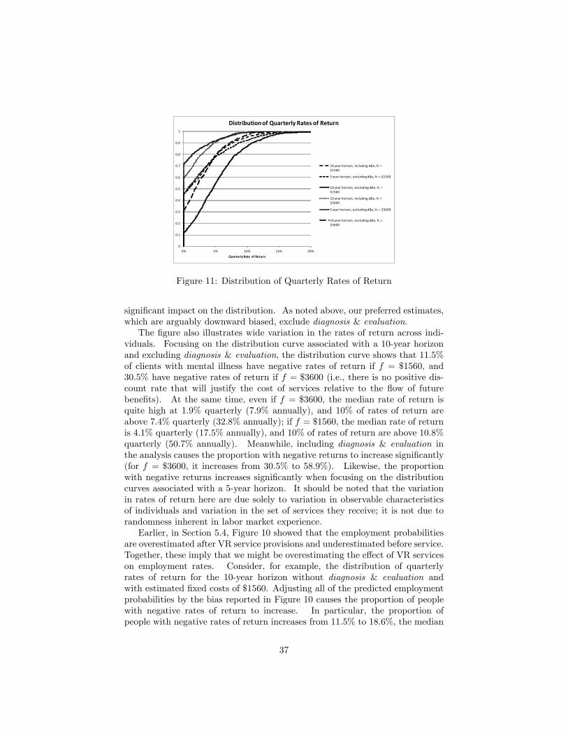
0

0.1

0.2

0.3

0.4

0.5

0.6

0.7

0.8

0.9

1

0% 5% 10% 15% 20%Quarterly Rate of Return

Distribution of Quarterly Rates of Return

10 year horizon, including d&e, fc =$1560

5 year horizon, excluding d&e, fc = $1560

10 year horizon, excluding d&e, fc =$1560

10 year horizon, including d&e, fc =$3600

5 year horizon, excluding d&e, fc = $3600

10 year horizon, excluding d&e, fc =$3600

Figure 11: Distribution of Quarterly Rates of Return

significant impact on the distribution. As noted above, our preferred estimates,which are arguably downward biased, exclude diagnosis & evaluation.

The figure also illustrates wide variation in the rates of return across indi-viduals. Focusing on the distribution curve associated with a 10-year horizonand excluding diagnosis & evaluation, the distribution curve shows that 11.5%of clients with mental illness have negative rates of return if f = $1560, and30.5% have negative rates of return if f = $3600 (i.e., there is no positive dis-count rate that will justify the cost of services relative to the flow of futurebenefits). At the same time, even if f = $3600, the median rate of return isquite high at 1.9% quarterly (7.9% annually), and 10% of rates of return areabove 7.4% quarterly (32.8% annually); if f = $1560, the median rate of returnis 4.1% quarterly (17.5% annually), and 10% of rates of return are above 10.8%quarterly (50.7% annually). Meanwhile, including diagnosis & evaluation inthe analysis causes the proportion with negative returns to increase significantly(for f = $3600, it increases from 30.5% to 58.9%). Likewise, the proportionwith negative returns increases significantly when focusing on the distributioncurves associated with a 5-year horizon. It should be noted that the variationin rates of return here are due solely to variation in observable characteristicsof individuals and variation in the set of services they receive; it is not due torandomness inherent in labor market experience.Earlier, in Section 5.4, Figure 10 showed that the employment probabilities

are overestimated after VR service provisions and underestimated before service.Together, these imply that we might be overestimating the effect of VR serviceson employment rates. Consider, for example, the distribution of quarterlyrates of return for the 10-year horizon without diagnosis & evaluation andwith estimated fixed costs of $1560. Adjusting all of the predicted employmentprobabilities by the bias reported in Figure 10 causes the proportion of peoplewith negative rates of return to increase. In particular, the proportion ofpeople with negative rates of return increases from 11.5% to 18.6%, the median

37

quarterly return decreases from 4.1% to 3.2% (13.4% annual rate of return), and10% of quarterly rates of return still are 8.8% (40.2% annual rate of return).However, this bias correction should be interpreted as suggestive because itdoes not control for other sources of bias and because we have not computedthe standard error of the bias correction.

7 Conclusions

Recently, there have been a number of state-level return on investment eval-uations of VR services produced by economic consulting firms or universityresearch bureaus (e.g., Heminway and Rohani, 1999; Uvin, Karaaslani, andWhite, 2004; Hollenbeck and Huang, 2006; Kisker et al., 2008; and Wilhelmand Robinson, 2010).46 By comparing outcomes of a “treated”and “untreated”group, as we do in Figures 4 and 5, these studies tend to find large positive re-turns to VR services. An evaluation of Utah’s VR program, for example, foundthat the public benefits of the program, measured in dollars, exceed the cost bya factor of 5.64 (Wilhelm and Robinson, 2010). These reports, however, have anumber of serious shortcomings which are addressed in this paper, including a)identification problems; b) problems caused by censored data; c) the selectionproblem; and d) heterogeneity in the caseload and in the services provided. Ouranalysis of the Virginia VR program addresses important limitations of theserecent studies. First, using the model described in Section 2, we formally ac-count for the possibility that selection into the treatment is endogenous. Asnoted above, a simple comparison of mean outcomes among treated and un-treated clients may be spurious due to selection, and conditioning on observedcovariates is not likely to address this problem credibly. Our results suggestthat selection plays an important role in inferences on the effect of VR services.Second, by focusing on clients with mental illnesses, we allow the estimatedeffects of treatment to vary with the clients’ limiting conditions. In contrast,these state-level reports do not distinguish between clients with mental illness,cognitive impairments, and physical impairments. Arguably, the effects of theprogram are heterogeneous, and restricting the impact to be constant across allgroups may lead to biased inferences. Third, unlike these earlier evaluations, weexamine the impact of specific types of services rather than just a single treat-ment indicator. We find that services do, in fact, have very different impacts onlabor market effects. Finally, we observe labor market and disability insuranceoutcomes many years before and after the provision of VR services. In thisanalysis, being able to estimate the long-run return is critical as it significantlydiffers from the short-run return.46These state level studies condition the analysis on observed covariates. In some cases (Hol-

lenbeck and Huang, 2006), researchers use statistical matching estimators based on propensityscores, initially developed by Rosenbaum and Rubin (1983) and incorporated in other man-power training program evaluations (e.g., Heckman, Ichimura, and Todd,1997; Dehejia andWahba, 1999). All of these analyses, however, invoke a conditional independence assumptionthat the outcome is independent of provision of services.

38

Our results suggest a complex picture of the impact of VR services on labormarket outcomes and DI/SSI receipt. Pre-program labor market differences varyacross the six service types, estimated employment effects are positive for someservices (e.g., training) and negative for others (e.g., education), and estimatedearnings effects are consistently positive. When combining the employment andearnings effects together, we find that, except for diagnosis & evaluation, allof the other service types have positive long-run effects. On average, training,restoration, and other services have benefits on the order of $7200, $3750, and$4800 respectively, while education and maintenance have positive benefits of$1700 and $2100 respectively. Overall, we find that VR services have a positiveaverage return, with mean long-run benefits of $4124 or $8374, depending uponhow one interprets diagnosis & evaluation results, and mean costs between$3460 and $5060. We also find, however, much variation in the return acrossVR participants. Depending upon how one estimates fixed costs (and excludingdiagnosis & evaluation), between 11.5% (f = $1560) and 30.5% (f = $3600) ofVR participants with mental illness have negative long-run rates of return, halfhave long-run annual rates of return in excess of between 17.5% (f = $1560)and 7.7% (f = $3600), and 10% have annual long-run annual rates of returnin excess of between 50.7% (f = $1560) and 32.8% (f = $3600). Finally,our results suggests that VR programs are unlikely to reduce the burgeoninggrowth in DI/SSI roles. To the contrary, we find that these services increase theprobability VR clients take-up DI/SSI.

References

[1] Aakvik, A., J. Heckman, and E. Vytlacil (2005). “Estimating TreatmentEffects For Discrete Outcomes When Responses To Treatment Vary: AnApplication to Norwegian Vocational Rehabilitation Programs.”Journal ofEconometrics. 125: 15-51.

[2] Arrighi, Y., B. Davin, A. Trannoy, and B. Ventelou (2010). “Un Effet Prixdans la Demande d’APA.”Unpublished manuscript.

[3] Ashenfelter, Orley (1978). “Estimating the Effect of Training Programs onEarnings.”Review of Economics and Statistics. 60: 47-57.

[4] Autor, David and Mark Duggan (2010). Supporting Work: A Proposal forModernizing the U.S. Disability Insurance System. Hamilton Project.

[5] Baldwin, Marjorie (1999). “The Effects of Impairments on Employmentand Wages: Estimates from the 1984 and 1990 SIPP.”Behavioral Sciencesand the Law. 17: 7-27.

[6] Baldwin, Marjorie (2005). “Explaining the Differences in Employment Out-comes Between Persons With andWithout Mental Disorders.”Unpublishedmanuscript.

39

[7] Bassi, L. (1984). “Estimating the Effect of Training with Non RandomSelection.”Review of Economics and Statistics. 66: 36-43.

[8] Bell, S., L. Orr, J. Blomquist, and G. Cain (1995). Program Applicants asa Comparison Group in Evaluating Training Programs. Upjohn Institutefor Employment Research.

[9] Bellante, D. (1972). “A Multivariate Analysis of a Vocational Rehabilita-tion Program.”Journal of Human Resources. 7: 226-241.

[10] Benitez-Silva, Hugo, Moshe Buchinsky, Hiu Man Chan, John Rust, andSofia Sheidvasser. (1999). “An Empirical Analysis of the Social SecurityApplication, Appeal and Award Process.”Labour Economics. 6: 147-178.

[11] Berkowitz, E. (1988). “The Cost-Benefit Tradition in Vocational Rehabili-tation.”Measuring the Effi ciency of Public Programs: Costs and Benefitsin Vocational Rehabilitation. (ed.) E. Berkowitz. Temple University Press,10-28.

[12] Bewley, Helen, Richard Dorsett, and Sergio Salis (2007). The Impact ofPathways to Work on Work, Earnings and Self-Reported Health in the April2006 Expansion Areas. Research Report No 601. Department for Work andPensions: London.

[13] Bond, G., R. Drake, and D. Becker (2001). “An Update on RandomizedControlled Trials of Evidence-Based Supported Employment.”PsychiatricRehabilitation Journal. 31(4): 280-290.

[14] Börsch-Supan, Axel and Vassilis Hajivassiliou (1992). “Health, Children,and Elderly Living Arrangements: A Multiperiod-Multinomial ProbitModel with Unobserved Heterogeneity and Autocorrelated Errors.”Top-ics in the Economics of Aging. (ed.) David Wise. Chicago and London: U.of Chicago Press, 79-104.

[15] Bratberg, E., A. Grasdal, and A. Risa. (2002). “Evaluating Social Policyby Experimental and Nonexperimental Methods.”Scandinavian Journal ofEconomics. 104(1): 147-171.

[16] Bureau of Economic Analysis (2010a). http://www.bea.gov/regional/docs/footnotes.cfm?tablename=CA04.

[17] Bureau of Economic Analysis (2010b). http://www.bea.gov/regional/docs/footnotes.cfm?tablename=CA25.

[18] Burns, Tom, Jocelyn Catty, Thomas Becker, Robert Drake, Angelo Fioritti,Martin Knapp, Christoph Lauber, Wulf Rössler, Toma Tomov, Jooske vanBusschbach, Sarah White, Durk Wiersma, Connie Geyer, Marsha Koletsi,Pascale Lissouba, Miles Rinaldi, Ulrike Ehiosun, Rana Kalkan, Reinhold

40

Kilian, Denise Manchisi, Astrid Niersman, Ingeborg Warnke, Dimitar Ger-manov, Adelina Comas, Claire Curran, and Anita Patel (2007). “The Effec-tiveness of Supported Employment for People with Severe Mental Illness:A Randomized Controlled Trial.”Lancet. 370(9593): 1146-1152.

[19] Butler, Richard, William Johnson, and Marjorie Baldwin (1995). “Man-aging Work Disability: Why First Return to Works is Not a Measure ofSuccess.”Industrial and Labor Relations Review. 48(3): 452-469.

[20] Campbell, Kikuko, Gary Bond, Robert Drake, Gregory McHugo, and HaiyiXie (2010). “Client Predictors of Employment Outcomes in High-FidelitySupported Employment: A Regression Analysis.”Journal of Nervous andMental Disease. 198(8): 556-563.

[21] Cimera, R. (2010). “The National Cost-Effi ciency of Supported Employeeswith Intellectual Disabilities: 2002 to 2007.”American Journal on Intel-lectual and Developmental Disabilities. 115: 19-29.

[22] Clapp, Christopher, Amalia Miller, John Pepper, and Steven Stern (2010).“Evaluation of Programs for High Risk Youth in Virginia.” Unpublishedmanuscript.

[23] Conley, R. (1969). “A Benefit Cost Analysis of the Vocational Rehabilita-tion Program." Journal of Human Resources. 4: 226-252.

[24] Cook, Judith, Anthony Lehman, Robert Drake, William McFarlane, PaulGold, H. Stephen Leff, Crystal Blyler, Marcia Toprac, Lisa Razzano, JaneBurke-Miller, Laura Blankertz, Michael Shafer, Susan Pickett-Schenk, andDennis Grey (2005). “Integration of Psychiatric and Vocational Services: AMultisite Randomized, Controlled Trial of Supported Employment.”Amer-ican Journal of Psychiatry. 162(10): 1948-1956.

[25] Currie, Janet and Bridget Madrian (1999). “Health, Health Insurance, andthe Labor Market.”Handbook of Labor Economics, Volume 3. (eds.) OrleyAshenfelter and David Card. Amsterdam : Elsevier.

[26] Dean, David and Robert Dolan (1991). “Fixed-Effects Estimates of Earn-ings Impacts for the Vocational Rehabilitation Program”Journal of HumanResources. 26(2): 380-391.

[27] Dean, David, Robert Dolan, and Robert Schmidt (1999). “Evaluating theVocational Rehabilitation Program Using Longitudinal Data: Evidence fora Quasi-experimental Research Design.”Evaluation Review. 23(2):162-189.

[28] Dean, David, Robert Dolan, Robert Schmidt, Paul Wehman, John Kregel,and Grant Revell (2002). “A Paradigm for Evaluation of the Federal-StateVocational Rehabilitation Program.”Achievements and Challenges in Em-ployment Services for People with Disabilities: The Longitudinal Impact ofWorkplace Supports. (eds.) John Kregel, David Dean, and Paul Wehman.

41

Richmond: Virginia Commonwealth University Rehabilitation Researchand Training Center on Workplace Supports.

[29] Dean, David, John Pepper, Robert Schmidt, and Steven Stern (2013a).“The Effects of Vocational Rehabilitation for People with Cognitive Im-pairments.”Unpublished manuscript.

[30] Dean, David, John Pepper, Robert Schmidt, and Steven Stern (2013b).“The Effects of Youth Transition Programs on Labor Market Outcomes.”Unpublished manuscript.

[31] Dehejia, R. and S. Wahba (1999). “Causal Effects in Non-ExperimentalStudies: Reevaluating the Evaluation of Training Programs.” Journal ofthe American Statistical Association. 94(448): 1053-1062.

[32] Doyle, Joseph (2007). “Child Protection and Child Outcomes: Measuringthe Effects of Foster Care.”American Economic Review. 97(5): 1583-1610.

[33] Drake, Robert, Jonathan Skinner, Gary Bond, and Howard Goldman(2009). “Social Security and Mental Illness: Reducing Disability With Sup-ported Employment.”Health Affairs. 28(3): 761-770.

[34] Ettner, Susan, Richard Frank, and Ronald Kessler (1997). “The Impact ofPsychiatric Disorders on Labor Market Outcomes.” Industrial and LaborRelations Review. 51(1): 64-81.

[35] French, Eric and Jae Song. (2012). “The Effect of Disability InsuranceReceipt on Labor Supply: A Dynamic Analysis.”Unpublished Manuscript.

[36] Friedlander, Daniel, David Greenberg, and Philip Robins (1997). “Evaluat-ing Government Training Programs for the Economically Disadvantaged.”Journal of Economic Literature. 35(4), 1809-1855.

[37] Frolich, M., A. Heshmati, and M. Lechner (2004). “A MicroeconometricEvaluation of Rehabilitation of Long-Term Sickness in Sweden.” Journalof Econometrics. 19: 375—396.

[38] Geweke, John (1988). “Antithetic Acceleration of Monte Carlo Integrationin Bayesian Inference.”Journal of Econometrics. 38(1/2): 73-89.

[39] Governmental Accountability Offi ce (2005) “Vocational Rehabilitation:Better Measures and Monitoring Could Improve the Performance of theVR Program.”Washington, D.C.

[40] Hanushek, Eric, John Kain, and Steven Rivkin (2002). “Inferring ProgramEffects for Special Populations: Does Special Education Raise Achievementfor Students with Disabilities?”Review of Economics and Statistics. 84(4):584-599.

42

[41] Heckman, J. and V. Hotz (1989). “Choosing Among Alternative Nonexper-imental Methods for Estimating the Impact of Social Programs: The Caseof Manpower Training.” Journal of the American Statistical Association.84: 862-874.

[42] Heckman, J., H. Ichimura, and P. Todd (1997). “Matching as an Economet-ric Estimator: Evidence from Evaluating a Job Training Program.”Reviewof Economic Studies. 65: 261-294.

[43] Heckman, James, Robert LaLonde, and Jeffrey Smith (1999). “The Eco-nomics and Econometrics of Active Labor Market Programs.”Handbookof Labor Economics Volume 3A. (eds.) Orley Ashenfelter and David Card.Amsterdam: North-Holland. 1865-2097.

[44] Heckman, James and Burton Singer (1984a). “Econometric DurationAnalysis.”Journal of Econometrics. 24: 63-132.

[45] Heminway, Derek and Faranak Rohani (1999). A Cost-Benefit Analysisof the Employment of People with Disabilities in Florida: Final Report.Educational Services Program.

[46] Hennessey, John and L. Scott Muller (1995). “The Effect of VocationalRehabilitation and Work Incentives on Helping the Disabled-Worker Ben-eficiary Back to Work.”Social Security Bulletin. 58(1): 15-28.

[47] Hollenbeck, Kevin and Wei-Jang Huang (2006). Net Impact and Benefit-Cost Estimates of the Workforce Development System in Washington State.Kalamazoo, MI: W.E. Upjohn Institute for Employment Research.

[48] Hotz, V. (1992). “Design Analysis Plan for the GAO Study of the Voca-tional Rehabilitation Program.”Correspondence with the GAO ProgramEvaluation and Methodology Division, 1-10.

[49] Imbens, Guido and Jeffrey Wooldridge (2009). “Recent Developments inthe Econometrics of Program Evaluation.”Journal of Economic Literature.47(1): 5—86.

[50] Keith, Samuel, Darrel Regier, and Donald Rae (1991). Psychiatric Dis-orders in America: The Epidemiologic Catchment Area Study. (eds.) LeeRobins and Darrel Regier. MacMillan: New York.

[51] Kessler, R., P. Berglund, M. Bruce, J. Koch, E. Laska, P. Leaf, R. Mander-scheid, R. Rosenheck, E. Walters, and P. Wang (2001). “The Prevalenceand Correlates of Untreated Serious Mental Illness.”Health Services Re-search. 36(6 Pt 1): 987-1007.

[52] Kimmel, Jean and Thomas Kniesner (1998). “New Evidence on Labor Sup-ply: Employment versus Hours Elasticities by Sex and Marital Status.”Journal of Monetary Economics. 42: 289-301.

43

[53] Kisker, E., G. Strech, J. Vetter, and C. Foote (2008). Evaluating Reha-bilitation Services in Oklahoma: An Analysis of Program Impacts and ofBenefit/Costs. Oklahoma Department of Rehabilitative Services.

[54] Kreider, Brent (1998). “Workers’ Applications to Social Insurance Pro-grams when Earnings and Eligibility are Uncertain.”Journal of Labor Eco-nomics. 16(4): 848-877.

[55] Kreider, Brent (1999). “Social Security Disability Insurance: Applications,Awards, and Lifetime Income Flows.”Journal of Labor Economics. 17(4):784-827.

[56] Kreider, Brent and John Pepper (2007). “Disability and Employment:Reevaluating the Evidence in Light of Reporting Errors.” Journal of theAmerican Statistical Association. 102(478): 432-41.

[57] LaLonde, Robert (1995). “The Promise of Public Sector-Sponsored Train-ing Programs.”Journal of Economic Perspectives. 9(2), 149-168.

[58] Loprest, P. (2007). Strategic Assessment of the State of the Science in Re-search on Employment for Individuals with Disabilities. National Institutefor Disability and Rehabilitation Research. Contract GS23F8198H.

[59] Maestas, Nicole, Kathleen Mullen, and Alexander Strand (2012). “DoesDisability Insurance Receipt Discourage Work? Using Examiner Assign-ment to Estimate Causal Effects of SSDI Receipt.” Unpublished manu-script.

[60] Marcotte D., V. Wilxox-Gok, and D. Redmond (2000). “The Labor MarketEffects of Mental Illness: The Case of Affective Disorders.”The Economicsof Disability. (eds.) D. Salkever and A. Sorkin. Greenwich, CT: JAI Press.

[61] McFadden, Daniel and Kenneth Train (2000). “Mixed MNL Models forDiscrete Response.”Journal of Applied Econometrics. 15(5): 447-470.

[62] McKeithen, Amelia and Steven Stern (2007). “The Costs and Benefits ofMental Healthcare.”http://www.people.virginia.edu/~sns5r/resint/psychtstf/mentalhealthbenefits.pdf.

[63] Meyer, Bruce (1995). “Natural and Quasi-Experiments in Economics.”Journal of Business and Economic Statistics. 13(2):151—162.

[64] Mueser, K., M. Salyers, and P. Mueser (2001). “A Prospective Analysis ofWork in Schizophrenia.”Schizophrenia Bulletin. 27: 281-296.

[65] Mueser, Peter, Kenneth Troske, and Alexey Gorislavky (2007). “UsingState Administrative Data to Measure Program Performance.”Review ofEconomics and Statistics. 89(4): 761-783.

44

[66] Nowak, L. (1983). “A Cost Effectiveness Evaluation of the Federal/StateVocational Rehabilitation Program Using a Comparison Group.” TheAmerican Economist. 27: 23-29.

[67] Raphael, Steven and Lorien Rice (2002). “Car Ownership, Employment,and Earnings.”Journal of Urban Economics. 52(1): 109-130.

[68] Raaum, O. and H. Torp (2001). “Labor Market Training in Norway —Ef-fects on Earnings.”Labour Economics. 8(5): 207-247.

[69] Rogers, J., M. Bishop, and M. Crystal (2005). “Predicting RehabilitationOutcome for Supplemental Security Income and Social Security DisabilityInsurance Recipients: Implications for Consideration with the Ticket toWork Program.”Journal of Rehabilitation. 71(3): 5-10.

[70] Rosenbaum, P. and D. Rubin (1983). “The Central Role of the PropensityScore in Observational Studies for Casual Effects.”Biometrika. 70: 41-55.

[71] Sosulski, Marya, Chandra Donnell, and Woo Jong Kim (2012). “Disabilityand Employee Benefits Receipt: Evidence from the U.S. Vocational Re-habilitation Services Program.” Journal of Social Work in Disability andRehabilitation. 11(1): 33-54.

[72] Stapleton, David and William Erickson (2004). Characteristics of Incen-tives: Why Do Employment Outcomes for the SSA Beneficiary Clients ofVR Agencies Differ, on Average, from Those of Other Clients? Washing-ton DC: Cornell University Institute for Policy Research.

[73] Stapleton, David and Frank Martin (2012). “Vocational Rehabilitationon the Road to Social Security Disability: Longitudinal Statistics fromMatched Administrative Data.”Unpublished manuscript.

[74] Stern, Steven (1992). “A Method for Smoothing Simulated Moments ofDiscrete Probabilities in Multinomial Probit Models.”Econometrica. 60(4):943-52.

[75] Stern, Steven (1997). “Simulation-Based Estimation.”Journal of EconomicLiterature. 35(4): 2006-2039.

[76] Stern, Steven (2010). “Moments and Extrema of Estimated Marginal Ef-fects for ‘The Effects of Vocational Rehabilitation for People with MentalIllness.”http://www.people.virginia.edu/~sns5r/resint/wrkdisstf/deanstruct.html.

[77] Tremblay, T., j. Smith, H. Xie, and R. Drake (2006). “Effect of BenefitsCounseling Services on Employment Outcomes for People with PsychiatricDisabilities.”Psychiatric Services. 57(6): 816-821.

45

[78] U.S. Dept. of Health and Human Services, Substance Abuse and Men-tal Health Services Administration (1999). “Estimation Methodology forAdults With Serious Mental Illness (SMI).” Federal Register. 64(121):33890-33897.

[79] U.S. Dept. of Health and Human Services, National Center for Health Sta-tistics (2004). National Health Interview Survey.

[80] Uvin, J., D. Karaaslani, and G. White (2004). Evaluation of Massachusetts’Public Vocational Rehabilitation Program: Final Report. Massachusetts Re-habilitation Commission.

[81] Wilhelm, S. and J. Robinson (2010). Utah State Offi ce of RehabilitationEconomic Impact Study. The University of Utah Center for Public Policyand Administration.

[82] Worrall, John (1978). “A Benefit-Cost Analysis of the Vocational Rehabil-itation Program.”Journal of Human Resources. 13: 285-298.

46