NBER WORKING PAPER SERIES

THE EFFECT OF AIR POLLUTION ON INVESTOR BEHAVIOR:EVIDENCE FROM THE S&P 500

Anthony HeyesMatthew NeidellSoodeh Saberian

Working Paper 22753http://www.nber.org/papers/w22753

NATIONAL BUREAU OF ECONOMIC RESEARCH1050 Massachusetts Avenue

Cambridge, MA 02138October 2016

Anthony Heyes receives ongoing financial support from the Canada Research Chair (CRC) program operated by the Government of Canada for his work in environmental economics. He is also part-time Professor of Economics at the University of Sussex. We are grateful to Josh Graff Zivin, Michaela Pagel, Juan-Pablo Montero, Roberton Williams III, Bernard Sinclair-Desgagne, Charles Mason and seminar participants at University of Paris, University of Wisconsin at Madison and CIRANO Montreal for constructive discussions. Errors are ours. The views expressed herein are those of the authors and do not necessarily reflect the views of the National Bureau of Economic Research.

NBER working papers are circulated for discussion and comment purposes. They have not been peer-reviewed or been subject to the review by the NBER Board of Directors that accompanies official NBER publications.

© 2016 by Anthony Heyes, Matthew Neidell, and Soodeh Saberian. All rights reserved. Short sections of text, not to exceed two paragraphs, may be quoted without explicit permission provided that full credit, including © notice, is given to the source.

The Effect of Air Pollution on Investor Behavior: Evidence from the S&P 500Anthony Heyes, Matthew Neidell, and Soodeh SaberianNBER Working Paper No. 22753October 2016JEL No. G02,J24,Q53

ABSTRACT

We provide detailed empirical evidence of a direct effect of air pollution on the efficient operation of the New York Stock Exchange, linking short-term variations in fine particulate matter (PM2.5) in Manhattan to movements in the S&P 500. The effects are substantial – a one standard deviation increases in ambient PM2.5 reduces same-day returns by 11.9% in our preferred specification – and remarkably robust to a variety of specifications and a battery of robustness and falsification checks. Furthermore, the intra-day effects that we observe are difficult to reconcile with competing hypotheses. Despite investors being dispersed geographically we find strong evidence that the effect is strictly local in nature, consistent with the high concentration of market influencers in New York. While we are agnostic as to the underlying mechanism, we provide evidence suggestive of the role of decreased risk tolerance operating through pollution-induced changes in mood or cognitive function.

Anthony HeyesDepartment of EconomicsUniversity of OttawaFaculty of Social Sciences120 University, Room 9029Ottawa CANADA K1N 6N5Anthony.Heyes@uottawa.ca

Matthew NeidellDepartment of Health Policy and ManagementColumbia University722 W 168th Street, 6th FloorNew York, NY 10032and NBERmn2191@columbia.edu

Soodeh SaberianDepartment of EconomicsUniversity of Ottawa120 University PrivateOttawa, Canada K1N 6N5saberian.soodeh@gmail.com

2

1. Introduction

Despite the long-standing theoretical appeal of the efficient market hypothesis

(Fama, 1965), researchers have uncovered significant empirical deviations from it.

Findings have included unexplained movements in aggregate prices, such as excessive

price volatility (Shiller, 1981) and the equity premium puzzle (Mehra and Prescott,

1985), inadequate incorporation of new information (Roll, 1984), the inexplicable role of

location specific factors (Froot and Dabora, 1999), and the influence of trader emotions

due to external stimuli (Saunders, 1993; Kamstra et al., 2003; Cueva at al., 2015).

Building on emerging economic evidence that links air pollution with a wide range of

human impacts, including cognition, mood and worker productivity (Graff Zivin and

Neidell, 2012; Chang et al., 2016; Lavy et al., 2014), we push this one step further by

looking at the effect of local air pollution on stock market returns. While we remain

largely agnostic on the precise mechanisms at play, we hypothesize that pollution

decreases the risk attitudes of investors via short-term changes in brain and/or physical

health.

Specifically, we estimate the effect of plausibly exogenous short-run changes in

fine particulate matter (PM2.5) in Manhattan over a 15 year period on daily returns of the

S&P 500, one of the most commonly used benchmarks for the overall New York Stock

Exchange (NYSE).2 The stocks quoted on the S&P 500 come from firms widely

differentiated by activity and geography, making it unlikely that daily variations in the

fundamentals that determine the fair value of those firms could be correlated with daily

2 Some recent correlational studies on air pollution and investor behavior include Lepori (2016), Li and Peng (2016), and Demir and Ersan (2016). Our analysis extends on this research through extensive attention to potential sources of confouding.

3

variations in air quality in the vicinity of Wall Street. We control flexibly for a wide

range of potentially-confounding meteorological considerations and other air pollutants

to isolate the effect of PM2.5 from competing environmental factors. Furthermore, by

controlling for time-specific factors using day of week fixed effects and year-by-week

fixed effects, our analysis excludes many additional potential confounding factors, such

as the well-established effect of length of day on investor mood (Kamstra et al., 2003).

We find a significant negative effect of PM2.5 on S&P 500 returns. In our

preferred specification, a one standard deviation increase in daily ambient PM2.5

concentrations causes a statistically significant 11.9% reduction in daily percentage

returns. The magnitude is comparable to estimates of the effect of variations in daily

weather conditions on returns (Goetzmann and Zhu, 2005; Hirshleifer et al., 2003). The

result proves remarkably robust to a variety of different assumptions about confounding

and a variety of falsification checks. We drill further into the data by conducting an intra-

day analysis. We find that PM2.5 concentrations throughout the day, but not the other

environmental variables, affect returns; this pattern is consistent with PM2.5 having indoor

penetration rates of over 90%, making it difficult to reconcile with competing hypotheses.

Critics of such local-based effects point out that any inefficient behavior by

Manhattan-based investors creates arbitrage opportunities for those located elsewhere.

This would imply our results are spurious, and air quality in New York City serves as a

proxy for more general changes in the fundamental value of stocks traded in the S&P

500. Since these stocks come from firms whose activities are widely dispersed across the

country and beyond, we can explore this threat by testing specifically for a local effect.

Using data from all pollution monitors across the U.S., we find that pollution in New

4

York City has by far the largest effect and is the only significant one. This makes it

implausible that unobserved variations in macroeconomic conditions – which could in

theory influence air quality and stock price movements simultaneously – are driving the

results. This points to the primacy of the attitudes of Manhattan-based market-makers, or

the particular concentration of investors and those exercising discretion in investment

decisions who work in and around Wall Street, in influencing price movements

(consistent with Goetzmann and Zhu, 2005).

Although several candidate mechanisms may explain the results, we investigate

the potential role that pollution-induced changes in risk aversion may play by examining

the effects of PM2.5 on movements in the volatility index (VIX). The VIX, which

measures the expected stock market volatility, is widely considered a measure of fear

amongst traders. We find that increases in PM2.5 lead to increases in the VIX.

Furthermore, decomposing the VIX into its risk and uncertainty elements, we find that

the effects only exist for the ‘pure’ risk aversion component. These findings suggest that

pollution-induced changes in risk appetite may be an important part of the story.

The results are important for at least two reasons. First, recent research on the

effect of pollution on worker productivity has focused either on work in outdoor settings

and/or in low skilled occupations (Graff Zivin and Neidell, 2012; Chang et al., 2016). As

such, the existing results are only pertinent for a small subset of employment in the U.S.

and comparably developed economies. By focusing on financial market professionals, we

extend this to include a set of indoor workers in a highly-skilled, cognitively-demanding

occupation, suggesting the detrimental effect of pollution on workplace performance is

even more widespread than previously believed.

5

Second, at a macroeconomic level, an effect of pollution on stock returns points to

another channel through which a polluted natural environment undermines the efficient

operation of a modern economy. Stock price variations send investment signals across the

whole of the U.S. and international economy - that is their purpose - and a well-

functioning stock market is a fundamental foundation for the efficiency claims made for

market-based economies. Thus, a significant impact of pollution upon daily returns

implies departure from the efficient markets hypothesis. In short, variations in air quality

in Manhattan – by affecting the investment sentiments of NYSE-based traders – causes

inefficient price signals rippling out across the wider economy.

The rest of the paper is laid out as follows. In Section 2 we review the evidence

that points to a link from individual exposure to PM2.5 to stock market returns. In Section

3 we outline data sources. In Section 4 we set out our empirical strategy. Section 5

presents the main results and those from a series of robustness checks. Section 6

concludes.

2. Pollution Exposure and Stock Market Returns

In order for daily local pollution levels to influence stock market returns on the

same day, a link from local pollution to an aspect of decision making relevant for stock

market returns must exist. In this section, we describe several mechanisms that might

underpin such a link. Though later we will have something to say about the possible role

of risk appetite, the contribution of this paper is not to choose between mechanisms, as a

number of the candidates might sensibly be expected to work in the same direction.

6

In brief, we posit that changes in air pollution have a variety of well-established

impacts on the human body and mind. These changes can affect investor decision making

via changes in factors such as risk appetite, choice bracketing behavior and mood. Such

changes in decisions by marginal investors or market-makers – physically located in New

York – affect movements in prices on the NYSE.

2.1. Pollution and health

We focus on fine particulate matter (PM2.5), which consists of solid and liquid

particles in the air less than 2.5 micrometers in diameter. Although natural sources, such

as forest fires, contribute to PM2.5 levels in New York City, the bulk of PM2.5 comes from

anthropogenic sources resulting from fossil fuel combustion by automobiles, industry,

and commercial and residential heat sources. According to the United States

Environmental Protection Agency, about 70% of PM2.5 in the city comes from sources

outside the urban area (US EPA 2004a, Figure 5), transported by wind and air

movements from the surrounding region.

Wall Street traders face PM2.5 exposure at various times during the day. Although

spending time outdoors, such as when traveling to work, is one important period of

exposure, indoor time is also pertinent. Given its diminutive size, PM2.5 easily enters

buildings, with penetration ranging from 70–100 percent (Thatcher and Layton, 1995;

Ozkaynak et al., 1996; Vette et al., 2001). Unlike other common air pollutants - which

either remain outside or break down very rapidly once indoors - going inside reduces

one’s exposure to PM2.5 only minimally.

7

The tiny sizes of the particles that make up PM2.5 also make this pollutant

particularly pernicious. It penetrates deep into human lungs and passes beyond into the

circulatory system to induce both respiratory and cardiovascular effects (Seaton et al.,

1995). A large body of toxicological and epidemiological evidence suggests that

exposure to PM2.5 harms a range of health outcomes (see US EPA 2004b for a review).

These risks may manifest themselves in clearly defined episodes, such as asthma attacks

and heart attacks, which lead to hospitalizations and mortality (Dockery and Pope, 1994;

Pope, 2000). They also lead to more subtle effects, such as changes in blood pressure,

irritation in the ear, nose, throat, and lungs, and mild headaches (Pope, 2000; Sorenson et

al., 2003); Ghio et al., 2000). These milder effects, which arise from exposure to lower

levels of PM2.5, are generally unobserved by the econometrician – they typically do not

lead to healthcare encounters – and in some cases may be largely unnoticed even by the

individual experiencing them. These more subtle effects may instead show up in, for

example, diminished work performance (Chang et al., 2016).

Symptoms from PM2.5 exposure can arise soon after exposure, but can also

sustain for hours and even days afterwards. This points to the need the need to allow for

contemporaneous and lagged effects of pollution in our analysis.

More recent evidence also links PM2.5 with cognitive effects. While cognitive

effects may arise indirectly through impaired respiratory functioning, a direct route exists

through changes in blood flow and circulation (Pope and Dockery, 2006). For example,

since the brain consumes a large fraction of the oxygen needs of the body, any

deterioration in blood supply can affect cognitive output (Clarke et al., 1999).

8

Furthermore, unlike other pollutants, the size of PM2.5 also allows it to travel up the

olfactory axon and enter the brain directly (Wang et al., 2007).

Empirical evidence documents cognitive effects on humans shortly after

exposure. Lavy et al. (2014) show that increased same-day PM2.5 in the vicinity of an

exam venue significantly decreases exam scores of Israeli students in the standardized

national Bagrut test. Archsmith et al. (2016) show that the decision-making accuracy of

Major League Baseball umpires falls as ambient PM2.5 in the vicinity of the baseball

stadium increases on game-day. In recent experimental evidence, Allen et al. (2016)

randomly assigned professional-grade employees to work in simulated office

environments with artificially manipulated indoor air quality.3 They found that cognitive

scores - particularly in the domains of ‘strategy’ and ‘information usage’ - declined

significantly on days with worse indoor air quality.

2.2. Health and decision making

The changes in health of the body and brain induced by pollution exposure can

affect decision-making in various ways. Indirectly, health can affect decision-making

through changes in resource allocation (Grossman, 1972). More directly, health can

affects one’s mood and emotions through the physical discomfort caused by the onset of

illness, which can affect decision making.

While the effects of cognition on some dimensions of decision-making are self-

evident – decision-making is in itself a cognitive function – there are additional channels

relevant for investor behavior. Dohmen et al. (2010) elicited measures of risk appetite 3 The study did not investigate PM2.5 directly but instead studied volatile organic compounds - a key precursor for PM2.5 in urban centers - and carbon dioxide.

9

and time preference, finding that risk appetite and degree of patience were increasing in

how well a subject scored in a cognitive task administered on the same day. While they

offer the theory of ‘choice bracketing’ – making decisions by comparing choices in

isolation rather than as a group – as an explanation for this effect (Tversky and

Kahneman, 1981), bracketing may also be part of the change in decision-making induced

by diminished cognition. For example, Rabin and Weizsacker (2010) and Abeler and

Marklein (2016) show that improved math performance, an important part of an

investor’s toolkit, reduces narrow bracketing.

2.3. Decision making and stock market returns

There is a well-established link from changes in risk aversion to financial decision

making. Increased risk aversion leads investors to shift away from risky assets such as

stocks, which lowers the returns on the market. An exogenous increase in risk aversion

among a subset of investors would be expected to reduce same-day return. This occurs as

the newly more risk averse investors move to reduce their risk exposure. Patience is also

long viewed as an essential ingredient in stock choices; it enables investors to focus on

the long term and ride out the short-run ups and downs. Similarly, choice bracketing can

also affect the type of stocks chosen as traders shift away from more complex choices

into simpler choices with lower returns.

More generally much of the recent behavioral finance literature focuses on the

emotional and visceral influences on financial behavior - how trading is influenced by

“how people are feeling.” The link from mood to stock returns has been the subject of a

large and robust literature; see Saunders (1993) and the subsequent studies. Central to

10

these articles is the notion that changes in mood induced by the weather affect the

decisions of investors, in particular inducing them to shift to safer bets. Again, the effect

of mood is conjectured to work through induced increases in risk aversion (see, for

example, Kamstra (2003)).

Last, it is worth making explicit that the proposed link hinges on the existence of

a local effect from air quality. Although many traders are physically present at the NYSE,

others are located elsewhere and trade electronically. Moreover, even those physically

present on the trading floor might be receiving instructions from people located anywhere

in the world. Consistent with Saunders (1993), we assume that the marginal investors

trade in New York, such that traders physically present can be expected to significantly

influence stock prices. In addition, even those geographically dispersed investors need to

contract with a physically present trader, and traders seek to affect prices in favor of their

investors (Hirshleifer et al., 2003).

A counter-acting effect is that the inefficient behavior of local investors creates an

arbitrage opportunity for investors outside the city (Goetzmann and Zhu, 2005; Loughran

and Schultz, 2004; Jacobsen and Marquering, 2008; Chang et al., 2008; Cao and Wei,

2005). To the extent that this counter-action were perfect we would see no net effect of

local air quality on aggregate returns, suggesting that the null hypothesis would prevail.

We will take great care to build a convincing case for a local effect of PM2.5

concentrations on stock market returns in the same location.

3. Data

The central part of our analysis exploits daily level data from a variety of sources.

11

3.1 Stock market returns

The main dependent variable of interest is the daily percentage returns on the U.S.

S&P 500. The S&P 500 index, the most widely-cited NYSE index, is designed to

measure performance of the broad domestic economy through changes in the aggregate

market value of 500 stocks representing all major industries.

We use the value-weighted daily records from January 2000 through November

2014 to compute the daily returns.4 We obtain the data on the S&P 500 from Datastream

(https://forms.thomsonreuters.com/datastream/). Table 1 shows the daily percentage

return of .025 over the sample period, a value comparable to previous estimates.

In our investigation of risk aversion as a potential mechanism we use the Chicago

Board Options Exchange (CBOE) Volatility Index (VIX). The VIX represents the

expected range of movement in the S&P 500 index over the next year. It is a widely used

proxy for market risk aversion, popularly referred to as the “fear index” or the “investor

fear gauge” (Coudert and Gex, 2008; Whaley, 2009). The daily VIX index data is

obtained from Factset (http://www.factset.com/) for the same dates as the S&P 500.

Table 1 also reports the daily mean VIX of 21.22.

Given the time-series nature of the data we first seek to verify the stationarity of

each series to rule out the possibility of spurious results due to time trends. We begin

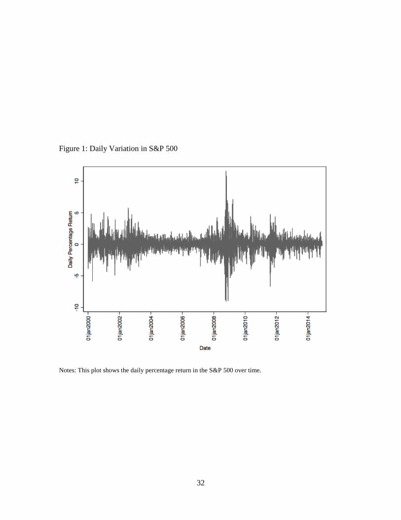
with a graphical analysis. Figure 1 plots the daily percentage return of the S&P 500 for

the study period. Although the plot shows significant activity around major stock events,

4 We begin our analysis in 2000 because this is when PM2.5 became routinely reported on a daily basis from the pollution monitor we use.

12

it appears stationary in pattern, a finding consistent with previous studies.5 The results of

a Dickey-Fuller test presented in Table 1 indicate that we can formally reject the null

hypothesis of the existence of a unit root. Likewise, Figure 2 plots the daily VIX price

for the study period. The increase in VIX around the financial crisis supports the

construct validity of this measure. Again there is no obvious drift present, a finding also

supported by the results of a Dickey-Fuller test presented in Table 1.

3.2 Air quality and weather

Air quality data is obtained from the New York State monitoring network

designed to comply with the federal regulations set forth by the US Environmental

Protection Agency. We collect hourly measures of PM2.5, carbon monoxide, and ozone at

the Division Street monitoring station in Lower Manhattan (monitor number 36-061-

0134), the station closest to the NYSE (located only 0.72 miles away).6

Weather data is obtained from two sources. Hourly observations for air

temperature, dew point, air pressure and wind speed are retrieved from the Air Quality

System (AQS) of the US Environmental Protection Agency. They are drawn from the

weather monitoring station at Susan Wagner High School, Staten Island (monitor number

36-085-0067), which is the closest station to the NYSE with consistent data throughout

our study period. Data for cloud cover and precipitation come from LaGuardia airport

5 We performed an analysis omitting the period of the financial crisis (October to December 2008 inclusive) and estimates were largely undisturbed. 6 In a robustness check instead of using the pollution measure from the closest air quality monitoring station we use a measure of Manhattan-average pollution levels by constructing an inverse distance-weighted average level of PM2.5 records at the three monitoring stations within 10 miles of the NYSE (until December, 2006, there were only two monitoring stations within 10 miles of the NYSE). Results using the Manhattan average were very close to those presented here.

13

monitoring station (monitor number USW00014732) of the Quality Controlled Local

Climatological Database of the National Oceanic and Atmospheric Administration

(NOAA).

For all environmental variables, we compute the daily average as the twenty-four

hour period from 4:00 PM to 3:59 PM to match the end of the NYSE trading day. Rather

than start the daily measure when the NYSE opens, we allow for the possible delay in

effects within a day from PM2.5 exposure, as the effects of PM2.5 take some time before

manifesting. This definition also excludes concentrations that arise after trading closes,

which logically can have no effect. In addition we perform a more flexible analysis by

using all environmental variables in two-hour blocks.

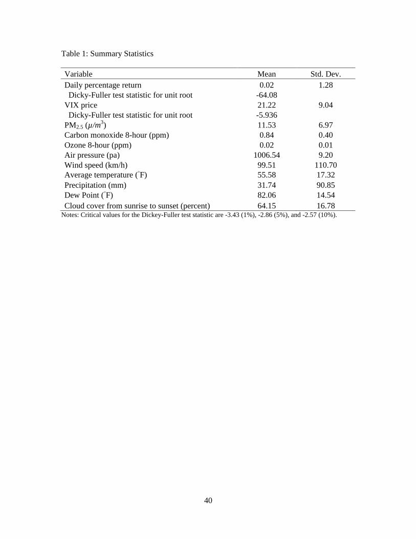
Table 1 presents summary statistics for all environmental variables. Air quality

has improved greatly in New York over time. The mean daily PM2.5 over the time period

is 11.53, below the annual air quality standards of 15 that applied at this time.7 The

maximum PM2.5 during this period is 75.86, with 66 days where daily values exceeded

the daily air quality standard of 35.

4. Econometric Model

To investigate the effect of PM2.5 levels on daily returns, we estimate the

following equation via ordinary least squares (OLS):

(1) rt = β0 + β1rt−1 + β2rt−2 + β3PM2.5t + Wtβ4 + Ptβ5 + Φt + εt.

7 The current annual standard is 12.0.

14

The variable rt is the S&P 500 percent return on date t. Following standard practice, we

include two lags of the dependent variables (rt−1 and rt−2) to control for any residual auto-

correlation.8 The independent variable of interest is the daily measure of fine particulate

matter, PM2.5. Our main interest lies in the parameter β3, which relates daily PM2.5 to

daily stock market returns.

Weather conditions are known to influence stock market returns. We control for

them in the vector Wt which contains temperature, dew point, precipitation, wind speed,

air pressure and cloud cover. The vector Pt contains measures of other pollutants that

might have an independent effect on returns: daily mean measures of 1-hour ozone and 8-

hour carbon monoxide.

The vector Φt contains various time fixed-effects. It includes day of the week

dummy variables to flexibly allow for different returns throughout the week. It also

includes a “tax dummy” that indicates the first five trading days and the last trading day

of the tax year to account for tax-loss selling.9 Moreover, it includes year-by-week

dummy variables to capture seasonality and other temporal patterns.10 Amongst other

things, the year-by-week dummy variables serve to control fully for any possible impact

of length of day on returns, of the sort studied by Kamstra et al. (2003) and pursuant

8 For examples see Goetzmann and Zhu, 2005; Loughran and Schultz, 2004; Jacobsen and Marquering, 2008; Chang et al., 2008; Kamstra et al., 2003; Saunders, 1993; Hirshleifer et al., 2003. 9 Consistent with the tax-loss selling hypothesis, US firms have been show to experience higher returns during the first few trading days of January (Reinganum, 1983). 10 The seasonality of stock market returns is well-established (Kamstra et al., 2012; Heston and Sadka, 2008; Wang et al., 1997; and Kohers and Patel, 1999). However, the results of Levy and Yagil, 2012; Brusa and Liu (2004) point to year-by-week dummies as the most appropriate controls in this setting.

15

literature. Finally, εt is an error term that allows for arbitrary serial correlation within a

week using Newey-West standard errors.11

Our main assumption for identifying β3 is that PM2.5 is uncorrelated with ε

conditional on the covariates included. One potential threat is that stock market returns

are driven by the fundamentals of a firm – none of which we observe – and

environmental policy affects these fundamentals (as well as PM2.5). For example,

complying with environmental policy might raise the general operating costs to a firm,

leading to worker layoffs and plant closure, but also lower pollution levels. While such an

argument might have credibility if we were studying annualized or other lower frequency

data, our focus on high-frequency (daily and even hourly) variation in PM2.5 eliminates

this concern. Also note that the firms that comprise the S&P500 have headquarters and

operations all over the country and the wider world. What we identify is a specifically

local effect, as we link air quality particular to New York to stock price movements, and

not air quality at other locations.

A second concern is that PM2.5 is correlated with other local environmental

influences that vary on a daily basis, such as weather and other pollutants. As already

noted, weather has a well-known relationship with stock returns. It is also seems

plausible that other pollutants might affect returns through similar mechanisms as PM2.5.

To limit this concern, we control directly for weather and co-pollutants in equation (1).

Furthermore, for temperature and humidity - which we expect to be the most likely

confounders - we control flexibly by way of a series of indicator ‘bins’ of width 2.5

degrees. This allows for possible threshold effects and other non-linearity in impacts. 11 Using different lengths of time for the Newey-West correction had a minimal impact on our standard errors.

16

Moreover, the year-by-week indicators also further control for weather to the extent that

it is constant within a week. For example, weather is highly serially correlated over a few

days, so controlling for the year-week allows us to compare different PM2.5 levels within

that small time period where weather remains stable. To further challenge the

specification we conduct a pair of further tests. First, a sensitivity analysis where we

exclude all meteorological variables and co-pollutant controls. Second, to further probe

the possibility that we are failing to adequately capture the effect of rain we re-estimate

our preferred specification on that subsample of days where realized precipitation was

zero.

We further isolate the role of PM2.5, as opposed to other daily varying

confounders, by performing intra-day analysis using hourly data. The advantage of this

specification is that, because the NYSE is a climate controlled environment, most

environmental factors do not penetrate indoors. Of the environmental factors we

consider, PM2.5 is the only one that penetrates effectively. Therefore, we would expect

weather and co-pollutant conditions at, say, 10am to have no effect on returns, whereas

PM2.5 levels at 10am should have an effect on returns, if it has an effect at all.12

The upper panel in Figure 3 plots daily PM2.5 levels and the lower panel the daily

PM2.5 residuals after controlling for weather controls and time dummies. The lower panel

makes clear that there is plenty of variation in pollution levels that is independent of

weather conditions. It is this variation that underpins our identification.

12 Our continued focus on daily returns is inconsequential for the hourly analysis: any effect on hourly returns should be reflected in daily returns. Note that we cannot predict the differential magnitude of the hourly effects since this would require us to know the speed at which exposure translates into changes in decision making.

17

5. Results

5.1 Main Results

Table 2 contains our main results, with the estimates in column 1 corresponding

with equation (1). The coefficient on PM2.5 of -.0171 is statistically significant at the 1%

level. This estimate indicates that a one unit increase in PM2.5 decreases the daily

percentage returns by 1.7%. Put differently, a one standard deviation increase in PM2.5

decreases the daily percentage returns by 11.9%, a substantial effect on daily NYSE

returns.

As PM2.5 can remain in the body for several days and may have a delayed effect

on health, in columns two and three we include one and two lags of PM2.5, respectively.

Since we are already controlling for lagged returns, this specification will capture any

cumulative effects to the extent they exist. Although the lags are also negative in

direction, they do not obtain statistical significance at conventional levels. Furthermore,

the contemporaneous effect remains more or less unchanged, suggesting the immediacy

of the effects of PM2.5 on returns.

As a falsification test, we add one and two leads of PM2.5. Pollution in the future

should not affect returns today, so finding an effect from future returns would suggest

model misspecification. Shown in columns four and five, we find that the coefficients on

the leads are small in size, mixed in sign, and never statistically significant. Again the

coefficient on contemporaneous PM2.5 remains more or less unchanged.

5.2 Sensitivity analysis

18

A concern already noted is the possible confounding role played by weather

variables and other pollutants. We already include a wide suite of controls (including

flexible controls for temperature and dew point) in the main specification, but to further

probe this issue we conduct three robustness checks, with the results summarized in

Table 3.

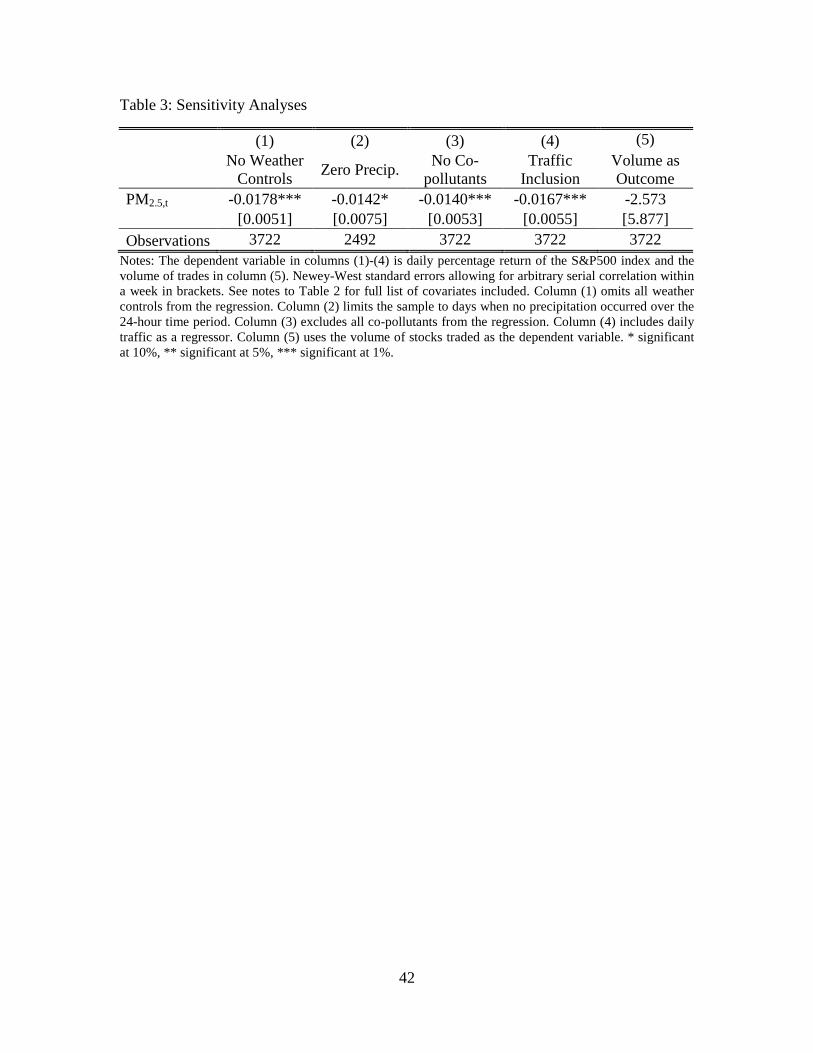
First, we exclude all weather variables entirely. If weather variables correlated

with PM2.5 are important confounders then omitting them should appreciably change our

results. The results of this exercise, summarized in column 1, shows minimal changes in

our estimates, from -.0171 to -.0178. This suggests that although weather may have an

influence on returns it is not in a way that is correlated with PM2.5.13 While we cannot

rule out some other unobserved meteorological confounder, the fact that omitting the six

major meteorological factors does not disturb our result limits this concern.

Second, we dig deeper into the possible confounding role of precipitation.

Precipitation may impact mood directly, and also plays an important role in influencing

PM2.5 levels. As a further check we conduct a sub-sample analysis by limiting ourselves

to days on which no precipitation occurred.14 The results, shown in column three, provide

an estimate of -.0145, again quite close to our original estimate. This suggests that

precipitation is unlikely to be a major source of confounding.

In column 3 we present the results of a third exercise, similar to the first except

now focusing on the role of co-pollutants. Since many pollutants have short-term health

impacts, and fossil fuels contribute to their formation, it is possible that we are falsely

13 We present the coefficients for weather in the appendix table and the hourly analysis. 14 Recall that we have defined a day not by the calendar but as the twenty four hour block of time from 4 PM one day to 4 PM the next.

19

attributing some of the effect of those to PM2.5. Again, although we cannot test whether

other, unobserved pollutants confound this relationship, we can test the extent to which

the pollutants we do observe confound this relationship. Excluding the co-pollutant

controls from the regression causes the estimate on our coefficient of interest to rise from

-.0171 to -.0205. This rather minimal change suggests that other pollutants are unlikely to

represent a source of omitted variable bias.

Another potential concern is the role of traffic; traffic increases pollution, but can

also lead to stress, which may affect returns. To assess this, we add to our regression

daily traffic data, obtained from the 3 traffic monitors located in Manhattan.15 Shown in

column (4) of Table 3, adding traffic scarcely affects the coefficient on PM2.5, suggesting

traffic is not a source of confounding.

An additional concern in interpreting our results is that the volume of stocks

traded may also change as a result of in response to pollution, potentially conflating our

estimates as both a volume and a price effect. To assess this possibility, we re-estimate

equation (1) using the volume of stocks traded as the dependent variable. Shown in

column (5) of Table 3, we find a small, statistically insignificant relationship between

PM2.5 and trade volume. Furthermore, if we include trade volume as a covariate in our

main specification, the coefficient on PM2.5 remains largely similar (not shown). These

results suggest that our results are capturing a pure price effect.

15 Continuous volume traffic data is obtained from the Department of Transportation (DOT) for the New York Metropolitan Transportation Council (NYMTC), available at https://www.dot.ny.gov/divisions/engineering/technical-services/highway-data-services/hdsb. The traffic monitors are Manhattan Span (id: 040920), Exit 29A Manhattan Bridge (id: 104745), and Manhattan Bridge Over (id: 127951).

20

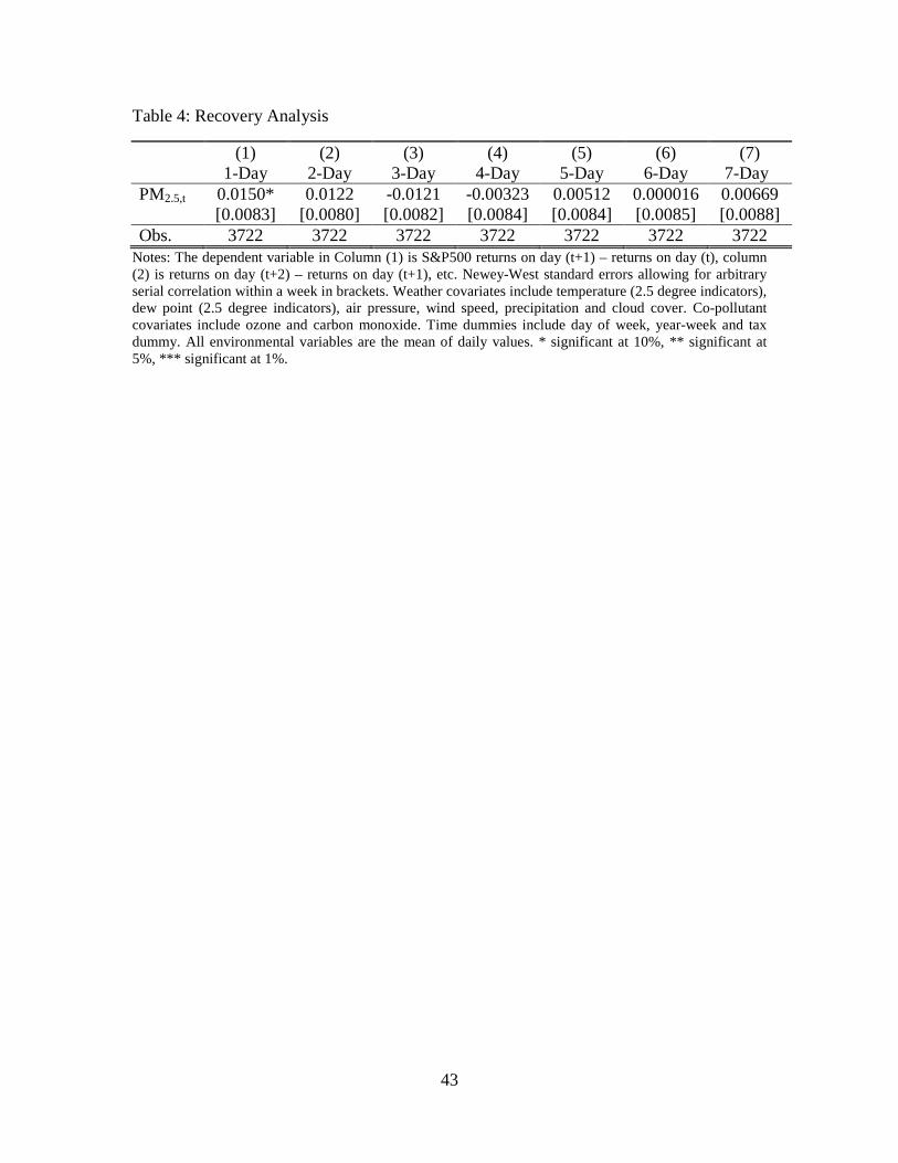
Although we hypothesize that PM2.5 affects stocks prices through investor

behavior, the fundamental value of each stock has not changed. Therefore, stock prices

should recover in the days after an increase in pollution occurs. To assess this, we replace

the dependent variable in equation (1) with future S&P 500 returns. If the stock market

recovers, then we expect pollution today to have a positive effect on returns in the future.

Table 4 presents results consistent with this. Returns on day t+1 are positive and

statistically significant, and completely offset the negative effect from day t. As we move

further into the future the coefficients are all statistically insignificant, and become

increasingly smaller in magnitude.

5.3 Placebo tests

A potential challenge to our inference is that unobserved macroeconomic changes

may impact both PM2.5 levels in New York and NYSE price movements. Exogenously

occurring positive macroeconomic news today might lead to both a rise in the price of

stocks and at the same time an increase in pollution in urban centers as real economic

activity expands. Failing to account for such news in our regression could lead us to

claim a spurious causal relationship from air pollution to stock price movements.

Although this seems unlikely given the high frequency of data used, to further limit any

such concerns we execute two placebo checks.16

First, we re-estimate our preferred specification 43 times, in each case replacing

the New York PM2.5 series with the analogous series from each of 43 other US cities. We

16 Note that macroeconomic fluctuations, to the extent they might bias our results, would likely bias them downward. Insofar as the story just told was to pass muster, it would imply a positive association between daily PM2.5 and stock price movements, whereas our analysis generates negative coefficients throughout.

21

chose those cities that (a) were over 250 miles from New York City and (b) were such

that data was available to provide daily measures for 80% of days in our study period.17

Insofar as macroeconomic variations mattered, we would expect these to be reflected in

air quality in cities across the country, not just in New York, and so would expect to

detect pollution levels in other locations affecting S&P 500 returns. The upper panel in

Figure 4 plots the estimated coefficients on the respective PM2.5 placebo series by city. 28

of the placebo series generate a positive coefficient, 15 negative. In terms of size all are

much smaller than the baseline estimate using the New York series – the next largest

coefficient is -.00646, which is a third of the size of our main estimate. The lower panel

plots the associated p-values for the placebo PM2.5 coefficients and show that none obtain

significance at the 10% level, and only a small number at the 20% level. Together this

leads us to conclude that the effect we identify is indeed a local one.

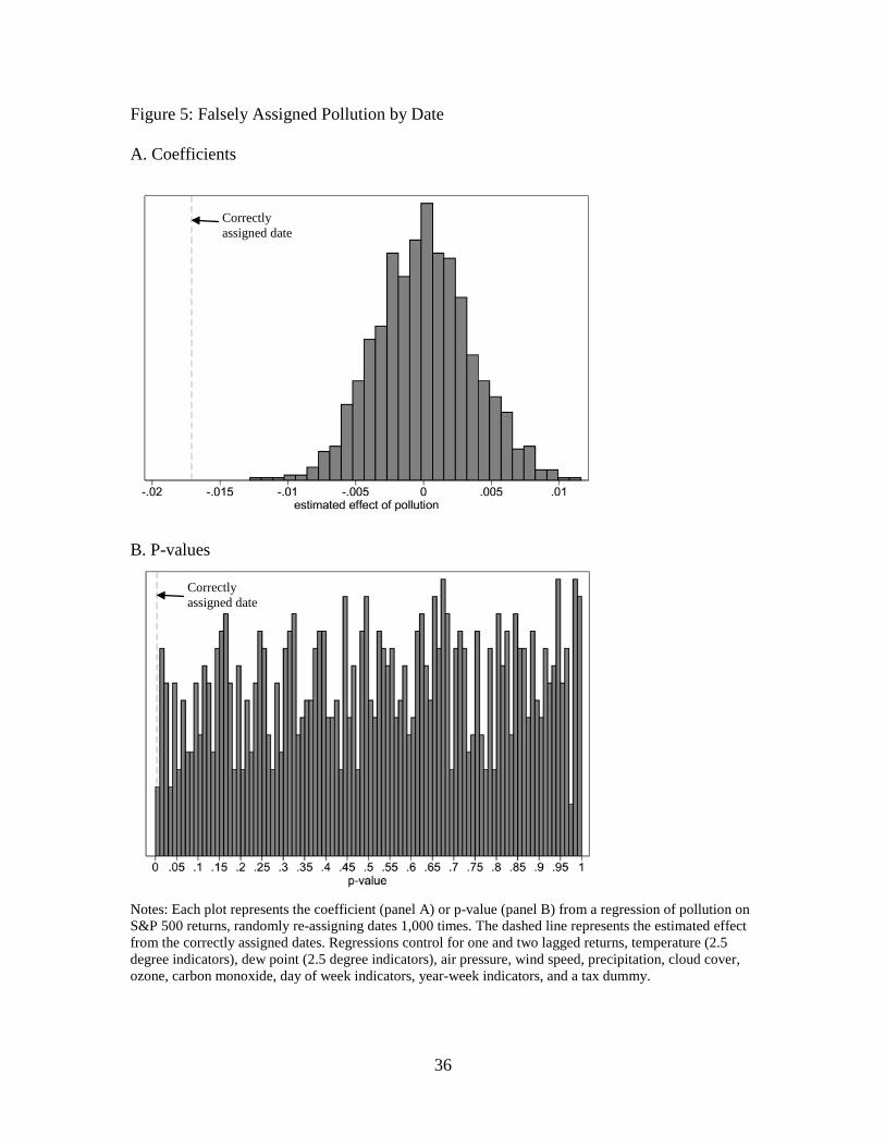
As a second test, we conduct a similar exercise by replacing the same-day New

York PM2.5 series with the series taken from that same city but on 1,000 different,

randomly-selected dates. We do this by randomly re-ordering the PM2.5 values within

New York, and re-estimating the preferred version of the model but using the falsely

assigned PM2.5 levels. Insofar as our claim of a contemporaneous effect of air quality on

investor behavior and stock market outcomes is valid, we would not expect this placebo

series to have significant explanatory power. Figure 5 confirms that this is indeed the

case. The upper panel plots the estimated coefficients on the placebo series, ordered by

magnitude. It can be seen that roughly half generate positive coefficients, half negative.

17 Some locations monitor PM2.5 every 3 or 6 days. We excluded cities less than 250 miles from New York because they could reasonably be affected by New York activity. Nonetheless, the estimates using data from these closer cities also supported our results (available upon request).

22

The lower panel again plots the associated p-values, and we observe that in 40 out of

1,000 cases the placebo series prove significant at the 5% level. This is roughly what we

would expect of the coefficient estimates obtained for a series of irrelevant regressors

inserted in turn into the regression.

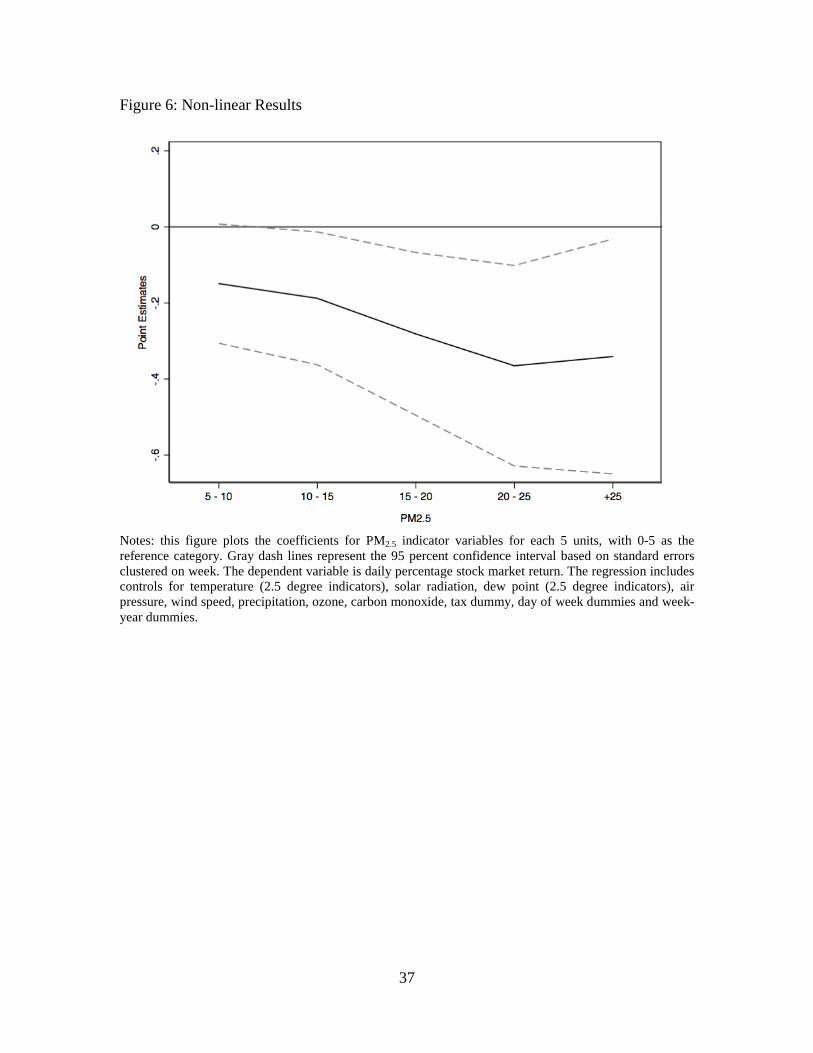
5.4 Non-linear estimates

In our baseline specification we have assumed a linear relationship between PM2.5

and investor behavior. We probe for possible non-linearity by including separate

indicators for every 5 µg/m3 of PM2.5 (with > 25 as the highest bin). In addition to

enabling us to test for any non-linearity, such as threshold effects, this also serves as a

robustness check: if PM2.5 affects returns, then higher levels of PM2.5 should have larger

effects. The results from this analysis, shown in Figure 6, while somewhat noisy,

generally support a linear effect of PM2.5 as the coefficients are nearly monotonically

increasing in PM2.5. Only estimates from the two highest bins are statistically significant,

though both are below the current daily air quality standard of 35 µg/m3. This suggests

that effects arise even when PM2.5 complies with environmental regulations.

5.5 Intra-day analysis

While the central results thus far presented rely on daily variations in pollution

and weather, the fine-grained nature of the data gives us the opportunity to explore intra-

day effects. Since exposure to the elements can have nearly immediate effects, we

investigate this by constructing average pollution and weather measures over two-hour

time blocks. Using these measures, we modify equation (1) as follows:

23

(2) rt = β0 + β1rt−1 + β2rt−2 + ∑jβ3jPM2.5tj + ∑jWtjβ4j + ∑jPtjβ5j + Φt + εt.

In this equation, we enter PM2.5, weather (W), and other pollutants (P) in two-hour

blocks, ranging from j = 12:00 AM – 1:59 AM to 10:00 PM to 11:59 AM.18

The key feature of this analysis is the difference in the ability of environmental

variables to penetrate indoors. Investors are largely outdoors when traveling to work at

the NYSE and thus exposed to all elements at that time. Once on the trading floor, the

climate-controlled environment in the NYSE significantly reduces exposure though does

not eliminate all sources. In fact, of the variables considered we only expect PM2.5 to

have an effect during the day because of its high indoor penetration rates.19 Therefore, we

only expect weather to affect traders during commuting hours while PM2.5 might affect

traders even once indoors.

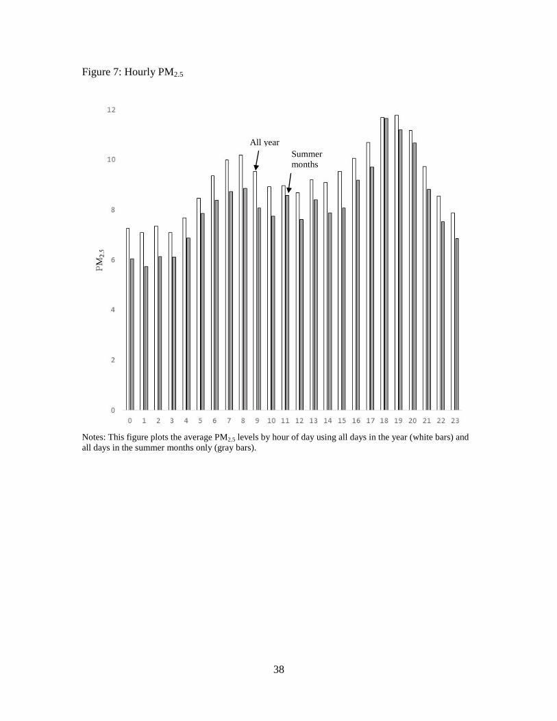
One concern with this analysis is whether there is sufficient independent variation

in hourly pollution. Figure 7 plots average hourly PM2.5, both for the entire year and only

for the summer months (July and August). Two immediate patterns suggest ample

variation in PM2.5. First, PM2.5 peaks at 8 AM and at 7 PM, a very different pattern from

temperature, which peaks midday. Second, PM2.5 levels decrease in the summer, again

very different from temperature, which increases in the summer.

18 To keep the number of coefficients feasible, we restrict all environmental variables to enter linearly. Note that solar radiation is entered daily rather than hourly. 19 For example, imagine a day that has a constant temperature of 85F and constant PM2.5 level of 10 µg/m3 every. As workers travel to the office they are exposed to both this temperature and PM2.5 level. Once workers reach the NYSE, the temperature to which they are exposed changes to that indoors at the climate-controlled exchange, while the PM2.5 to which they are exposed remains approximately unchanged.

24

Note that we cannot predict the relative magnitudes of the hourly PM2.5 responses

for three reasons. One, penetration rates are not 100%, and we do not have measures of

indoor PM2.5 at the exchange. Two, although the effects from PM2.5 can be expected to

reveal themselves in the first few hours after exposure, we cannot pinpoint the exact time

at which it affects workers. Three, there may be cumulative effects from PM2.5 exposure

within the day that we cannot disentangle with an additively separable model.20

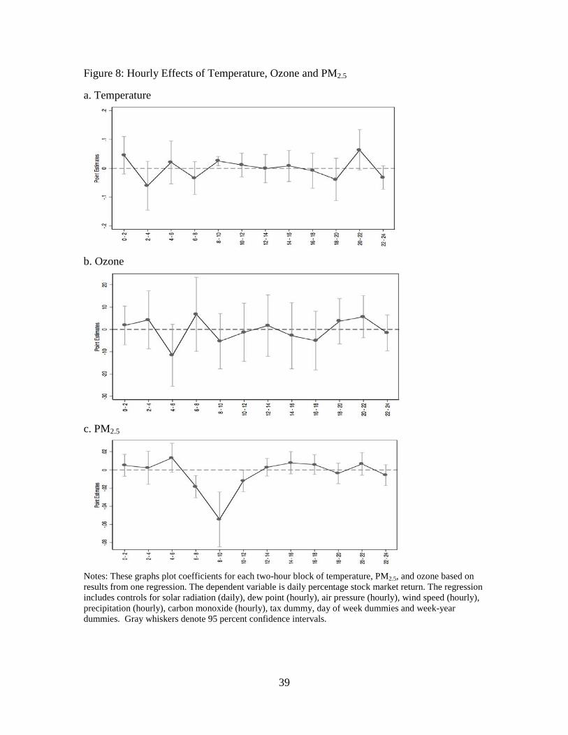
In Figure 8 we display estimates from equation 2 for the hourly measures of

PM2.5, temperature and ozone.21 Several findings stand out. First, consistent with prior

literature, temperature has a significant and positive effect, but only from 8 – 10 AM,

prime commuting hours. Warmer temperature on the journey to work - the usual story

would say - improves mood, reduces risk aversion and so in turn increases daily returns.

Second, ozone, a pollutant that does not penetrate indoors (and is not generally believed

to have cognitive effects) is never statistically significant. Third, PM2.5 has a statistically

significant effect from 6 – 8 AM, 8 – 10 AM, and 10 AM – 12 PM, which include a

period after traders and most other financial professionals are at work. The effect

becomes considerably smaller throughout the afternoon, possibly reflecting the delay

with which PM2.5 affects the body. Last, as expected we do not see effects in the evening

hours after the exchange has closed, a finding consistent with our lead tests from Table 2.

These hourly results further support our contention that PM2.5 has a causal effect on stock

market returns.

20 A richer model with interactions terms is not feasible given the number of additional variables and the correlation in PM2.5 through the day. 21 Intra-day results for all environmental variables are available upon request.

25

5.6 Exploring risk aversion as mechanism

In Section 2 we summarized research that potentially links human exposure to

PM2.5 to decreased returns via increased risk aversion. Though we recognize the

possibility of other mechanisms - and indeed it may be that several mechanisms are at

work simultaneously - in this section we probe the idea that pollution-induced changes in

risk appetite may be playing a role by using data on the VIX index, a widely used proxy

for market risk aversion (Coudert and Gex, 2008); Whaley, 2009).

We estimate our main regressions using the VIX index as the dependent variable.

Our hypothesis of risk aversion as a potential mechanism underpinning our central results

would imply a positive coefficient on PM2.5. Table 5 reports the results from this analysis,

repeating the structure in Table 2. Consistent with our hypothesis, we find that PM2.5 has

a statistically significant positive relationship with the VIX. It implies that a one unit

increase in PM2.5 concentration increases the value of VIX by 1.9%. Similar to our

previous results, we find that adding leads and lags of PM2.5 does not substantially alter

our findings.

While the VIX is commonly used as a proxy for risk aversion, it reflects both

changes in taste for risk and in anticipated market volatility. We decompose the overall

measure into these two elements, referred to as the ‘risk aversion’ and ‘uncertainty’

components, respectively (Bekaert et al., 2013).22 The results of re-estimation using each

of those components as dependent variables in turn are presented in Table 6. They

indicate that PM2.5 significantly increases the pure risk aversion component, but is

22 Following Bekeart et al (2013) we regress realized variance (computed using daily percentage returns) on the 22-day lagged squared VIX and realized variance. The fitted value from this regression is the estimated measure of ‘uncertainty’ and the residual is our ‘risk aversion’ proxy.

26

statistically unrelated to the uncertainty component. Sensitivity analyses including leads

and lags (not shown) mirror previous results that only contemporaneous PM2.5 matters.23

While not definitive, these results support pollution-induced risk aversion as a possible

mechanism linking changes in PM2.5 to changes in stock market returns.

6. Conclusion

The efficient markets hypothesis is a central tenet of neoclassical economics. We

provide the first empirical evidence of a causal link from air quality and the efficient

operation of financial markets. In particular, poor air quality in the city in which a stock-

market is based causes market prices to diverge from prices based on fundamentals.

When Manhattan-based traders are exposed to higher levels of PM2.5, the return on the

S&P 500 on that day is lowered. This is consistent with an induced fall in risk appetite

among a subset of traders, plausible given existing research on the role short-term

exposure to air pollution can have on brain health, cognition and risk attitude. The effects

are economically significant - a one standard deviation increases in ambient PM2.5

concentrations reduces same-day returns by 11.9% in our preferred specification - and

prove robust to a variety of specifications and a battery of robustness and falsification

checks. In the daily analysis which is central in the paper we take particular care to

isolate the role of pollution from weather factors - already known to affect mood and

trading behavior - using a variety of methods. Furthermore, the intra-day effects that we

observe are difficult to reconcile with competing hypotheses.

23 Results are also robust to the confounding sensitivity analysis done in Table 3.

27

Investors are widely dispersed. There is however a very strong concentration of

those who exercise financial discretion working in offices in New York - not just those

trading at the NYSE but wealth managers and other market-influencers more generally

(for example Blackrock, the world’s largest wealth management company is Manhattan-

based). Furthermore the market-making activities are largely New York based. As such

we were particularly careful to investigate the geography of the effect. The results point

to a strictly local effect, as pollution levels in a wide set of other American cities are

unrelated to S&P 500 returns. This also rules out that the analysis is picking up

unaccounted for variations in macroeconomic circumstances that contemporaneously

influence stock market and pollution levels across cities.

The results can be seen as interesting on a number of levels. First, they provide

further evidence of the ubiquitous influence that the natural environment has on

important social and economic outcomes. Variations in the quality of air in Manhattan

systematically distort investment signals being sent out across the whole economy.

Second, if we consider returns as a metric for the productivity of an NYSE trader, the

results point to a detrimental effect of diminished air quality on the work performance of

this class of employee, so significantly extending the insight of recent research showing

similar impacts on the productivity of low-skilled workers.

28

7. Bibliography

Abeler, J. and F. Marklein (2016). Fungibility, Labels and Consumption. Forthcoming Journal of the European Economic Association. Allen, J. G., P. MacNaughton, U. Satish, S. Santanam, J. Vallarino and J. D. Spengler (2016). Associations of Cognitive Function Scores with Carbon Dioxide, Ventilation and Volatile Organic Compound Exposure in Office Workers: A Controlled Exposure Study of Green and Conventional Office Environments. Environmental Health Perspective 124(6). Archsmith, J., A. Heyes, A. and S. Saberian (2016). Air Quality and Error Quantity: Pollution and Performance in a High-skilled, Quality-focused Occupation. Mimeograph, Department of Economics, University of California at Davis. Bekaert, G., M. Hoerova and M. L. Duca (2013). Risk, Uncertainty and Monetary Policy. Journal of Monetary Economics 60(7): 771–788. Benjamin, D. J., O. Heffetz, M. S. Kimball and A. Rees-Jones (2012). What Do You Think Would Make You Happier? What Do You Think You Would Choose? American Economic Review 102(5): 2083–2110. Bouman, S. and B. Jacobsen (2002). The Halloween Indicator, ‘Sell in May and Go Away’: Another Puzzle. American Economic Review 92(5): 1618–1635. Brusa, J. and P. Liu (2004). The Day-of-the-week and the Week-of-the-month Effect: An Analysis of Investors’ Trading Activities. Review of Quantitative Finance and Accounting 23(1): 19–30. Campbell, J. Y., S. Grossman and J. Wang (1993). Trading Volume and Serial Correlation in Stock Returns. Quarterly Journal of Economics 108(4): 905–940. Chang, S., S. Chen, R. K. Chou and Y. H. Lin (2008). Weather and Intraday Patterns in Stock Returns and Trading Activity. Journal of Banking and Finance 32(9): 1754–1766. Chang, T., J. Graff Zivin, T. Gross, T. and M. J. Neidell (2016). Particulate Pollution and the Productivity of Pear Packers. Forthcoming American Economic Journal: Economic Policy. Cao, M. and J. Wei (2005). An Expanded Study on the Stock Market Temperature Anomaly. Research in Finance 22: 73–112. Clarke, D. and L. Sokoloff (1999). Circulation and Energy Metabolism of the Brain, Chapter 31 in Eds. G. Siegel and B. Agranoff, Basic Neurochemistry (sixth edition) Raven Press: New York.

29

Coudert, V. and M. Gex (2008). Does Risk Aversion Drive Financial Crises? Testing the Predictive Power of Empirical Indicators. Journal of Empirical Finance 15(2): 167–184. Cueva, C., R. E. Roberts, T. Spencer, N. Rani, M. Tempest, P. Tobler and A. Rustichini (2015). Cortisol and Testosterone Increase Financial Risk-taking and May Destabilize Markets. Nature (Scientific Reports) Article Number 11206. Demir, Ender and Oguz Ersan (2016). “When stock market investors breathe polluted air.” Entrepreneurship, Business and Economics 2: 705-720. Dockery, D. W. and C. A. Pope (1994). Acute Respiratory Effects of Particulate Air Pollution. Annual Review of Public Health 15(1): 107–132. Dohmen, T. J., A. Falk, D. Huffman and U. Sunde (2010). Are Risk Aversion and Impatience Related to Cognitive Ability? American Economic Review 3(100): 1238–1260. Eisenberg, T., S. Sundgren and M. T. Wells (1998). Larger Board Size and Decreasing Firm Value in Small Firms. Journal of Financial Economics 48(1): 35–54. Fama, Eugene (1965). “The Behavior of Stock-Market Prices.” The Journal of Business 38(1) Froot, Kenneth and Emil Dabora (1999). “How are stock prices affected by the location of trade?” Journal of Financial Economics 53(2). Ghio, A. J., C. Kim and R. B. Devlin (2000). Concentrated Ambient Air Particles Induce Mild Pulmonary Inflammation in Healthy Human Volunteers. American Journal of Respiratory and Critical Care Medicine 162(3): 981–988. Goetzmann, W. N. and N. Zhu (2005). Rain or Shine: Where is the Weather Effect? European Financial Management 11(5): 559–578. Grossman, M. (1972). On the Concept of Health Capital and the Demand for Health. Journal of Political Economy 80(2): 223–255. Guiso, L., P. Sapienza and L. Zingales (2014). The Value of Corporate Culture. Journal of Financial Economics 117(1): 60–76. Hirshleifer, D. and T. Shumway (2003). Good Day Sunshine: Stock Returns and The Weather. Journal of Finance 58(3): 1009–1032. Jacobsen, B. and W. Marquering (2008). Is it the Weather? Journal of Banking and Finance 32(4): 526–540. Kamstra, M. J., L. A. Kramer and M. D. Levi (2012). A Careful Re-examination of

30

Seasonality in International Stock Markets: Comment on Sentiment and Stock Returns. Journal of Banking and Finance 36(4): 934–956. Kamstra, M. J., L. A. Kramer and M. D. Levi (2003). Winter Blues: A SAD Stock Market Cycle. American Economic Review 93(1): 324–343. Kelly, P. J. and F. Meschke, F. (2010). Sentiment and Stock Returns: The SAD Anomaly Revisited. Journal of Banking and Finance 34(6): 1308–1326. Kohers, T. and J. B. Patel (1999). A New Time-of-the-month Anomaly in Stock Index Returns. Applied Economics Letters 6(2): 115–120. Lavy, V., A. Ebenstein and S. Roth (2014). “The Impact of Short Term Exposure to Ambient Air Pollution on Cognitive Performance and Human Capital Formation.” NBER Working Paper #20648. Lepori, Gabriele (2016). “Air pollution and stock returns: Evidence from a natural experiment.” Journal of Empirical Finance 35: 25-42. Levy, T. and J. Yagil (2012). “The Week-of-the-year Effect: Evidence from Around the Globe.” Journal of Banking and Finance 36(7): 1963–1974. Li, Q. and C.H. Peng (2016). “The stock market effect of air pollution: evidence from China.” Applied Economics 48(36): 3442-3461. Loughran, T. and P. Schultz (2004). Weather, Stock Returns and the Impact of Localized Trading Behavior. Journal of Financial and Quantitative Analysis 39(02): 343–364. Mehra, R. and E. C. Prescott (1985). “The Equity Premium: A Puzzle.” Journal of Monetary Economics 15 (2). Ozkaynak, H., J. Xue, J. Spengler, L. Wallace, E. Pellizzari and P. Jenkins (1995). Personal Exposure to Airborne Particles and Metals: Results from the Particle TEAM Study in Riverside, California. Journal of Exposure Analysis and Environmental Epidemiology 6(1): 57–78. Pope III, C. A. (2000). Epidemiology of Fine Particulate Air Pollution and Human Health: Biologic Mechanisms and who is at Risk? Environmental Health Perspectives 108(4): 713–723. Pope III, C. A. and D. W. Dockery (2006). Health Effects of Fine Particulate Air Pollution: Lines that Connect. Journal of the Air and Waste Management Association 56(6): 709–742. Rabin, M. and G. Weizsacker (2009). Narrow Bracketing and Dominated Choices. American Economic Review 99(4): 1508–1543.

31

Reinganum, M. R. (1983). The Anomalous Stock Market Behavior of Small Firms in January: Empirical Tests for Tax-loss Selling Effects. Journal of Financial Economics 12(1): 89–104. Roll, Richard (1984). “Orange Juice and Weather.” American Economic Review 74(5). Saunders, E. M. (1993). Stock Prices and Wall Street Weather. American Economic Review 83(5): 1337–1345. Seaton, A., D. Godden, W. MacNee and K. Donaldson (1995). Particulate Air Pollution and Acute Health Effects. Lancet 345(8943): 176–178. Shiller, Robert (1981). ““Do Stock Prices Move Too Much to Be Justified by Subsequent Changes in Dividends?” American Economic Review 71(3). Smoski, M. J., A. Rittenberg and G. S. Dichter (2011). Major Depressive Disorder is Characterized by Greater Reward Network Activation to Monetary than Pleasant Image Rewards. Psychiatry Research: Neuroimaging 194(3): 263–270. Thatcher, T. L. and D. W. Layton (1995). Deposition, Resuspension and Penetration of Particles Within a Residence. Atmospheric Environment 29(13): 1487–1497. Tversky, A. and D. Kahneman (1981). The Framing of Decisions and the Psychology of Choice. Science 211(4481): 453–458. United States Environmental Protection Agency (2004a). The Particle Pollution Report: Current Understanding of Air Quality and Emissions Through 2003. Office of Air Quality Planning and Standards. Research Triangle Park, North Carolina. United States Environmental Protection Agency (2004b). Air Quality Criteria for Particulate Matter. National Center for Environmental Assessment (NCEA). Research Triangle Park, North Carolina. Vette, A. F., A. Rea, P. Lawless, C. E. Rhodes, G Evans, V. R. Highsmith and L. Sheldon (2001). Characterization of Indoor-outdoor Aerosol Concentration Relationships During the Fresno PM Exposure Studies. Aerosol Science and Technology 34(1): 118–126. Wang, K., Y. Li and Erickson (1997). A New Look at the Monday Effect. Journal of Finance 52(5): 2171–2186. Whaley, R. E. (2009). Understanding the VIX. Journal of Portfolio Management 35(3): 98–105.

32

Figure 1: Daily Variation in S&P 500

Notes: This plot shows the daily percentage return in the S&P 500 over time.

33

Figure 2: Daily Variation in VIX

Notes: This plot shows the daily VIX price over time.

34

Figure 3: Daily Variation in PM2.5

Notes: The upper panel plots unadjusted daily PM2.5. The bottom panel plots PM2.5 adjusted for temperature (2.5 degree indicators), dew point (2.5 degree indicators), air pressure, wind speed, precipitation, cloud cover, ozone, carbon monoxide, day of week indicators, year-week indicators, and a tax dummy.

35

Figure 4: Falsely Assigned Pollution by City A. Coefficients

B. P-values

Notes: Each circle represents the coefficient (panel A) or p-value (panel B) from a regression of that city’s pollution on S&P 500 returns, controlling for one and two lagged returns, temperature (2.5 degree indicators), dew point (2.5 degree indicators), air pressure, wind speed, precipitation, cloud cover, ozone, carbon monoxide, day of week indicators, year-week indicators, and a tax dummy.

New York

New York

36

Figure 5: Falsely Assigned Pollution by Date A. Coefficients

B. P-values

Notes: Each plot represents the coefficient (panel A) or p-value (panel B) from a regression of pollution on S&P 500 returns, randomly re-assigning dates 1,000 times. The dashed line represents the estimated effect from the correctly assigned dates. Regressions control for one and two lagged returns, temperature (2.5 degree indicators), dew point (2.5 degree indicators), air pressure, wind speed, precipitation, cloud cover, ozone, carbon monoxide, day of week indicators, year-week indicators, and a tax dummy.

Correctly assigned date

Correctly assigned date

37

Figure 6: Non-linear Results

Notes: this figure plots the coefficients for PM2.5 indicator variables for each 5 units, with 0-5 as the reference category. Gray dash lines represent the 95 percent confidence interval based on standard errors clustered on week. The dependent variable is daily percentage stock market return. The regression includes controls for temperature (2.5 degree indicators), solar radiation, dew point (2.5 degree indicators), air pressure, wind speed, precipitation, ozone, carbon monoxide, tax dummy, day of week dummies and week-year dummies.

38

Figure 7: Hourly PM2.5

Notes: This figure plots the average PM2.5 levels by hour of day using all days in the year (white bars) and all days in the summer months only (gray bars).

All year Summer months

39

Figure 8: Hourly Effects of Temperature, Ozone and PM2.5

a. Temperature

b. Ozone

c. PM2.5

Notes: These graphs plot coefficients for each two-hour block of temperature, PM2.5, and ozone based on results from one regression. The dependent variable is daily percentage stock market return. The regression includes controls for solar radiation (daily), dew point (hourly), air pressure (hourly), wind speed (hourly), precipitation (hourly), carbon monoxide (hourly), tax dummy, day of week dummies and week-year dummies. Gray whiskers denote 95 percent confidence intervals.

40

Table 1: Summary Statistics Variable Mean Std. Dev. Daily percentage return 0.02 1.28 Dicky-Fuller test statistic for unit root -64.08 VIX price 21.22 9.04 Dicky-Fuller test statistic for unit root -5.936 PM2.5 (µ/m3) 11.53 6.97 Carbon monoxide 8-hour (ppm) 0.84 0.40 Ozone 8-hour (ppm) 0.02 0.01 Air pressure (pa) 1006.54 9.20 Wind speed (km/h) 99.51 110.70 Average temperature (◦F) 55.58 17.32 Precipitation (mm) 31.74 90.85 Dew Point (◦F) 82.06 14.54 Cloud cover from sunrise to sunset (percent) 64.15 16.78

Notes: Critical values for the Dickey-Fuller test statistic are -3.43 (1%), -2.86 (5%), and -2.57 (10%).

41

Table 2: Main Regression Results for the Effect of Pollution on S&P 500 Returns

(1) (2) (3) (4) (5)

Daily 1-Day Lag 2-Day Lag 1-Day Lead 2-Day Lead PM2.5,t -0.0168*** -0.0166*** -0.0180*** -0.0174*** -0.0178***

[0.0055] [0.0055] [0.0054] [0.0055] [0.0055]

PM2.5,t-1 - -0.0042 -0.0033 - -

- [0.0047] [0.0044] - -

PM2.5,t-2 - - -0.0044 - -

- - [0.0053] - -

PM2.5,t+1 - - - 0.0028 0.0033

- - - [0.0045] [0.0046]

PM2.5,t+2 - - - - -0.0021

- - - - [0.0043]

Observations 3722 3722 3722 3722 3722 Time Dummies Y Y Y Y Y

Weather Y Y Y Y Y Co-pollutants Y Y Y Y Y

Notes: The dependent variable is daily percentage return of the S&P500 index. Newey-West standard errors allowing for arbitrary serial correlation within a week in brackets. Weather covariates include temperature (2.5 degree indicators), dew point (2.5 degree indicators), air pressure, wind speed, precipitation and cloud cover. Co-pollutant covariates include ozone and carbon monoxide. Time dummies include day of week, year-week and tax dummy. All environmental variables are the mean of daily values. * significant at 10%, ** significant at 5%, *** significant at 1%.

42

Table 3: Sensitivity Analyses

(1) (2) (3) (4) (5)

No Weather Controls Zero Precip. No Co-

pollutants Traffic

Inclusion Volume as Outcome

PM2.5,t -0.0178*** -0.0142* -0.0140*** -0.0167*** -2.573

[0.0051] [0.0075] [0.0053] [0.0055] [5.877]

Observations 3722 2492 3722 3722 3722 Notes: The dependent variable in columns (1)-(4) is daily percentage return of the S&P500 index and the volume of trades in column (5). Newey-West standard errors allowing for arbitrary serial correlation within a week in brackets. See notes to Table 2 for full list of covariates included. Column (1) omits all weather controls from the regression. Column (2) limits the sample to days when no precipitation occurred over the 24-hour time period. Column (3) excludes all co-pollutants from the regression. Column (4) includes daily traffic as a regressor. Column (5) uses the volume of stocks traded as the dependent variable. * significant at 10%, ** significant at 5%, *** significant at 1%.

43

Table 4: Recovery Analysis

(1) (2) (3) (4) (5) (6) (7)

1-Day 2-Day 3-Day 4-Day 5-Day 6-Day 7-Day

PM2.5,t 0.0150* 0.0122 -0.0121 -0.00323 0.00512 0.000016 0.00669

[0.0083] [0.0080] [0.0082] [0.0084] [0.0084] [0.0085] [0.0088]

Obs. 3722 3722 3722 3722 3722 3722 3722 Notes: The dependent variable in Column (1) is S&P500 returns on day (t+1) – returns on day (t), column (2) is returns on day (t+2) – returns on day (t+1), etc. Newey-West standard errors allowing for arbitrary serial correlation within a week in brackets. Weather covariates include temperature (2.5 degree indicators), dew point (2.5 degree indicators), air pressure, wind speed, precipitation and cloud cover. Co-pollutant covariates include ozone and carbon monoxide. Time dummies include day of week, year-week and tax dummy. All environmental variables are the mean of daily values. * significant at 10%, ** significant at 5%, *** significant at 1%.

44

Table 5: The Effect of Pollution on the Volatility Index

(1) (2) (3) (4) (5) Daily 1-Day Lag 2-Day Lag 1-Day Lead 2-Day Lead

PM2.5,t 0.0198** 0.0202** 0.0209** 0.0207** 0.0218** [0.0056] [0.0057] [0.0057] [0.0056] [0.0058] PM2.5,t-1 - -0.0075 -0.0079 - - - [0.0051] [0.0051] - - PM2.5,t-2 - - 0.0021 - - - - [0.0051] - - PM2.5,t+1 - - - -0.0042 -0.0067 - - - [0.0049] [0.0048] PM2.5,t+2 - - - - -0.0094

- - - - [0.0048] Observations 3722 3722 3722 3722 3722 Time Dummies

Y Y Y Y Y

Weather Y Y Y Y Y Co-pollutants Y Y Y Y Y Notes: The dependent variable is daily volatility index (VIX). Newey-West standard errors allowing for arbitrary serial correlation within a week in brackets. Weather covariates include temperature (2.5 degree indicators), dew point (2.5 degree indicators), air pressure, wind speed, precipitation and cloud cover. Co-pollutant covariates include ozone and carbon monoxide. Time dummies include day of week, year-week and tax dummy. All environmental variables are the mean of daily values. * significant at 10%, ** significant at 5%, *** significant at 1%.

45

Table 6: Pollution and the VIX Components: Risk Aversion and Uncertainty

(1) (2) (3) (4) (5) (6) Daily 1-Day Lag 2-Day Lag Daily 1-Day Lag 2-Day Lag Risk Aversion Uncertainty PM2.5,t

0.0870*** 0.0873*** 0.0911*** -0.0062 -0.0061 -0.0059

[0.0263] [0.0267] [0.0271] [0.0046] [0.0046] [0.0047] PM2.5,t-1 - -0.00585 -0.00813 - -0.0027 -0.0028 - [0.0281] [0.0281] - [0.0046] [0.0047] PM2.5,t-2 - - 0.0116 - - 0.00037 - - [0.0249] - - [0.0039] Obs. 3700 3700 3700 3700 3700 3700 Time Dummies

Y Y Y Y Y Y

Weather Y Y Y Y Y Y Co-pollutants

Y Y Y Y Y Y

Notes: The dependent variable is VIX separated into risk aversion (column 1-3) and uncertainty (column 4-6) components. Newey-West standard errors allowing for arbitrary serial correlation within a week in brackets. Weather covariates include temperature (2.5 degree indicators), dew point (2.5 degree indicators), air pressure, wind speed, precipitation and cloud cover. Co-pollutant covariates include ozone and carbon monoxide. Time dummies include day of week, year-week and tax dummy. All environmental variables are the mean of daily values. * significant at 10%, ** significant at 5%, *** significant at 1%.