1

This is the authors’ accepted manuscript of an article

published in the Journal of Business. The definitive version is

available at:

http://www.jstor.org/page/journal/jbusiness/about.html

2

The Effect of Asymmetries on Optimal Hedge

Ratios*

Chris Brooks

The ISMA Centre, Department of Economics, University of Reading

Ólan T. Henry

Department of Economics, University of Melbourne,

Gita Persand

The ISMA Centre, Department of Economics, University of Reading

3

Abstract

There is widespread evidence that the volatility of stock

returns displays an asymmetric response to good and bad news.

This paper considers the impact of asymmetry on time varying

hedges for financial futures. An asymmetric model which allows

forecasts of cash and futures return volatility to respond

differently to positive and negative return innovations gives

superior in-sample hedging performance. However, the simpler

symmetric model is not inferior in a hold-out sample. A method

for evaluating the models in a modern risk management

framework is presented, highlighting the importance of allowing

optimal hedge ratios to be both time-varying and asymmetric.

4

1. Introduction

Over the past two decades, increases in the availability and usage of

derivative securities has allowed agents who face price risk the opportunity to

reduce their exposure. Although there are many techniques available for

reducing and managing risk, the simplest and perhaps the most widely used, is

hedging with futures contracts. A hedge is achieved by taking opposite

positions in spot and futures markets simultaneously, so that any loss

sustained from an adverse price movement in one market should to some

degree be offset by a favourable price movement in the other. The ratio of the

number of units of the futures asset that are purchased relative to the number

of units of the spot asset is known as the hedge ratio.

Since risk in this context is usually measured as the volatility of

portfolio returns, an intuitively plausible strategy might be to choose that

hedge ratio which minimises the variance of the returns of a portfolio

containing the spot and futures position; this is known as the optimal hedge

ratio. There has been much empirical research into the calculation of optimal

hedge ratios (see, for example, Cecchetti et al., 1988; Myers and Thompson,

1989; Baillie and Myers, 1991; Kroner and Sultan, 1991; Lien and Luo, 1993;

Lin et al., 1994; Strong and Dickinson, 1994; Park and Switzer, 1995).

The general consensus is that the use of multivariate generalised

autoregressive conditionally heteroscedastic (MGARCH) models yields

superior performances evidenced by lower portfolio volatilities, than either

time-invariant or rolling ordinary least squares (OLS) hedges. Cecchetti et al

(1988), Myers and Thompson (1989) and Baillie and Myers (1991), for

example, argue that commodity prices are characterised by time-varying

5

covariance matrices. As news about spot and futures prices arrives to the

market, the conditional covariance matrix, and hence the optimal hedging

ratio, becomes time-varying. Baillie and Myers (1991) and Kroner and Sultan

(1993), inter alia, employ MGARCH models to capture time-variation in the

covariance matrix and the resulting hedge ratio.

On the other hand, there is also evidence that the benefits of a time

varying hedge are substantially diminished as the duration of the hedge is

increased (e.g Lin et al., 1994). Moreover, there is evidence that the use of

volatility forecasts implied by options prices can further improve hedging

effectiveness (Strong and Dickinson, 1994).

This paper has three main aims. Firstly, we link the concept of the

optimal hedge with the notion of the News Impact Surface of Kroner and Ng

(1998). The hedging surface of the OLS model is independent of news

arriving to the market and therefore could be sub-optimal. Secondly, we

extend the models of Cecchetti et al (1988), Myers and Thompson (1989) and

Baillie and Myers (1991) to allow for time variation and asymmetry across the

entire variance covariance matrix of returns. This means that the hedge ratio

will be sensitive to the size and sign of the change in prices resulting from

information arrival. Thirdly, we adapt the methods used by Hsieh (1993) to

show how the effectiveness of hedges can be evaluated by the calculation of

minimum capital risk requirements (MCRRs). Such a procedure allows the

hedging performance of the various models to be assessed using a relevant

economic loss function as well as on pure statistical grounds.

The paper is laid out in six sections. Section two presents the

theoretical framework for deriving the hedge ratios, while section three

6

describes the data. Section four presents the empirical evidence on the

performance of each hedging model, while the fifth section outlines the

bootstrap methodology used to calculate the MCRR for each of the portfolios.

Section six concludes.

2. The Derivation of Optimal Hedge Ratios

Let tC and tF represent the logarithms of the stock index and stock

index futures prices respectively. The actual return on a spot position held

from time tt to1 is 1 ttt CCC similarly, the actual return on a futures

position is 1 ttt FFF . However, at time 1t , the expected return,

)(1 tt RE , of the portfolio comprising one unit of the stock index and units of

the futures contract may be written as

Et-1(Rt) = Et-1 (Ct)- t-1Et-1 (Ft) (1)

where t-1 is the hedge ratio determined at time t-1, for employment in period

t.1 The variance of the portfolio may be written as

CFtttFttCtp hhhh 1,

2

1,, 2 (2)

where tph , , tFh , and tCh , represent the conditional variances of the portfolio

and the spot and futures positions respectively and tCFh , represents the

conditional covariance between the spot and futures position. If the agent has

the two moment utility function

tptttptt hREhREU ,1,1 )(),( (3)

then the utility maximising agent with degree of risk aversion seeks to solve

)2(

),(max

,1,

2

1,11

,1

tCFttFttCttttt

tptt

hhhFECE

hREU

(4)

7

Solving (4) with respect to under the assumption that tF is a martingale

process such that 0)( 11111 ttttttt FFFFEFE yields *

1t , the

optimal number of futures contracts in the investor’s portfolio

tF

tCF

th

h

,

,*

1 (5)

If the conditional variance-covariance matrix is time-invariant (and if tC and

tF are not cointegrated) then an estimate of *, the constant optimal hedge

ratio, may be obtained from the estimated slope coefficient b in the regression

ttt uFbaC (6)

The OLS estimate of b = hCF / hF is also valid for the multiperiod hedge in the

case where the investors utility function is time separable.

However, it has been shown by numerous studies (see section 1 above)

that the data do not support the assumption that the variance-covariance matrix

of returns is constant over time. Therefore we follow recent literature by

employing a bivariate GARCH model which allows the conditional variances

and covariances used as inputs to the hedge ratio to be time-varying.

In the absence of transactions costs, market microstructure effects or

other impediments to their free operation, the efficient markets hypothesis and

the absence of arbitrage opportunities implies that the spot and corresponding

futures markets react contemporaneously and identically to new information.

There has been some debate in the literature as to whether this implies that the

two markets must be cointegrated. Ghosh (1993), for example, suggests that

market efficiency should imply that cash and futures are cointegrated, while

Baillie and Myers (1991) suggest that, as a consequence of possible non-

stationarity of the risk free proxy employed in the cost of carry model, this

8

need not be the case. We do not wish to enter into this debate from a

theoretical viewpoint, but suffice to say that in all ensuing analysis, we allow

for, but do not impose, a [-1 1] cointegrating vector for the two series. The

conditional mean equations of the model employed in this paper are a bivariate

Vector Error Correction Mechanism (VECM), which may be written as

tC

tF

t

C

F

C

Ci

C

Fi

F

Ci

F

Fi

i

C

F

t

t

t

ttit

i

it

C

FY

vYY

,

,

)(

,

)(

,

)(

,

)(

,

1

4

1

;;;;

(7)

Under the assumption ),0(~| ttt H , where t represents the

innovation vector in (6) and defining ht as vech(Ht), where vech(.) denotes the

vector-half operator that stacks the lower triangular elements of an NN

matrix into an 1)2/)1(( NN vector, the bivariate VECM(p) GARCH(1,1)

vech model may be written

where

Restricting the matrices A1 and B1 to be diagonal gives the model

proposed by Bollerslev, Engle and Wooldridge (1988) where each element of

the conditional variance-covariance matrix hij,t depends on past values of itself

and past values of '

11 tt . There are 21 parameters in the conditional

vec H h

h

h

h

C A vec B ht t

C t

CF t

F t

t t t( ) ( ' )

,

,

,

0 1 1 1 1 1 (8)

333231

232221

131211

1

333231

232221

131211

1

22

12

11

0 ;;

bbb

bbb

bbb

B

aaa

aaa

aaa

A

c

c

c

C

9

variance-covariance structure of the bivariate GARCH(1,1) vech model (8) to

be estimated, subject to the requirement that Ht be positive definite for all

values of t in the sample. The difficulty of checking, let alone imposing such

a restriction led Engle and Kroner (1995) to propose the BEKK

parameterisation

*

111

*'

11

*

11

'

11

*'

11

*

0

*'

0 BHBAACCH tttt (9)

The BEKK parameterisation requires estimation of only 11 parameters in the

conditional variance-covariance structure and guarantees Ht positive definite.

It is important to note that the BEKK and vec models imply that only the

magnitude of past return innovations is important in determining current

conditional variances and covariances. This assumption of symmetric time-

varying variance-covariance matrices must be considered tenuous given the

existing body of evidence documenting the asymmetric response of equity

volatility to positive and negative innovations of equal magnitude (see Engle

and Ng, 1993, Glosten, Jagannathan and Runkle, 1993, and Kroner and Ng,

1998, inter alia).

Defining 0,min, ttj , for j=futures, cash, the BEKK model in (9)

may be extended to allow for asymmetric responses as

*

11

'

11

*'

11

*

111

*'

11

*

11

'

11

*'

11

*

0

*'

0 DDBHBAACCH tttttt (10)

where

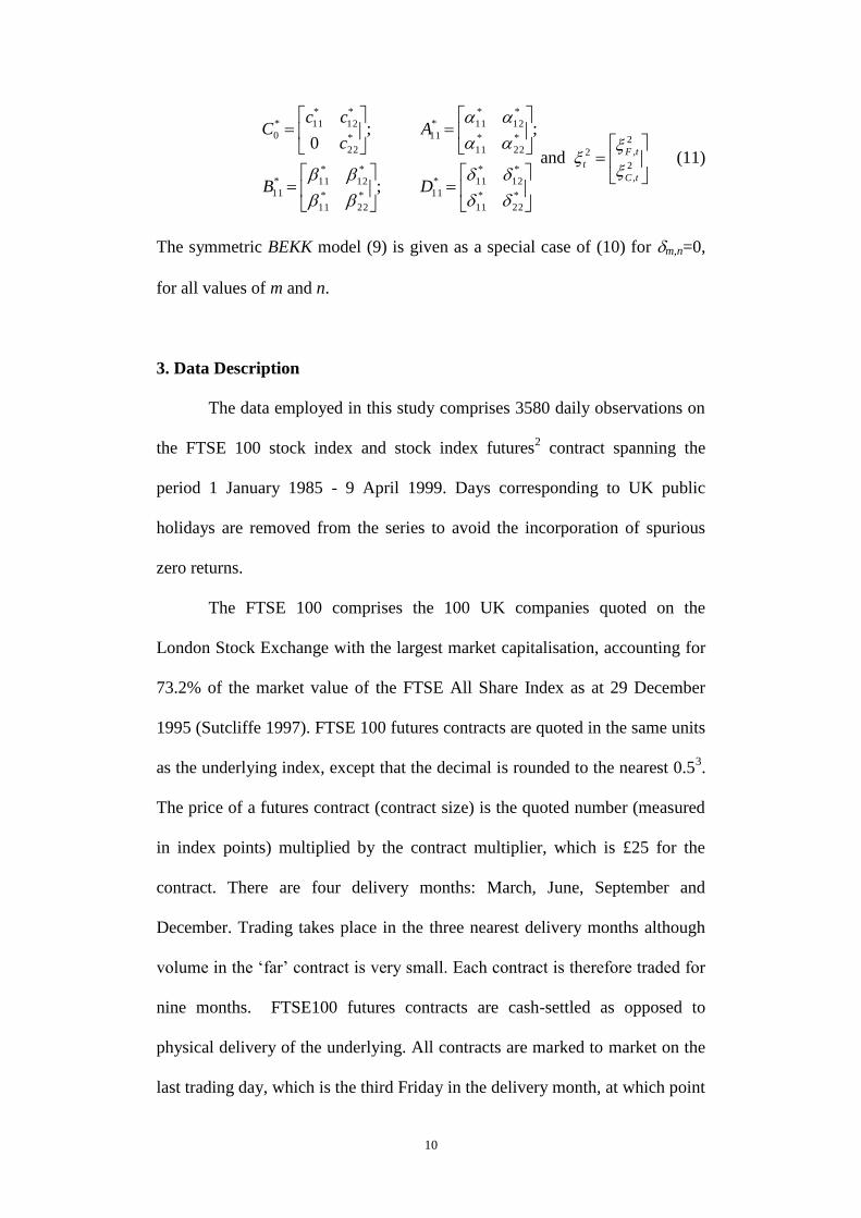
10

*

22

*

11

*

12

*

11*

11*

22

*

11

*

12

*

11*

11

*

22

*

11

*

12

*

11*

11*

22

*

12

*

11*

0

;

;;0

DB

Ac

ccC

and

2

,

2

,2

tC

tF

t

(11)

The symmetric BEKK model (9) is given as a special case of (10) for m,n=0,

for all values of m and n.

3. Data Description

The data employed in this study comprises 3580 daily observations on

the FTSE 100 stock index and stock index futures2 contract spanning the

period 1 January 1985 - 9 April 1999. Days corresponding to UK public

holidays are removed from the series to avoid the incorporation of spurious

zero returns.

The FTSE 100 comprises the 100 UK companies quoted on the

London Stock Exchange with the largest market capitalisation, accounting for

73.2% of the market value of the FTSE All Share Index as at 29 December

1995 (Sutcliffe 1997). FTSE 100 futures contracts are quoted in the same units

as the underlying index, except that the decimal is rounded to the nearest 0.53.

The price of a futures contract (contract size) is the quoted number (measured

in index points) multiplied by the contract multiplier, which is £25 for the

contract. There are four delivery months: March, June, September and

December. Trading takes place in the three nearest delivery months although

volume in the ‘far’ contract is very small. Each contract is therefore traded for

nine months. FTSE100 futures contracts are cash-settled as opposed to

physical delivery of the underlying. All contracts are marked to market on the

last trading day, which is the third Friday in the delivery month, at which point

11

all positions are deemed closed. For the FTSE100 futures contract, the

settlement price on the last trading day is calculated as an average of minute-

by-minute observations between 10:10AM and 10:30AM rounded to the

nearest 0.5.

Summary statistics for the data are displayed in panel A of table 1.

Using Dickey Fuller (1979) unit root tests, it is not possible to reject the null

hypothesis of non-stationarity for the cash and futures price series. This non-

stationarity of the price series is consistent with weak-form efficiency of the

cash and futures markets. The return series are calculated as )/(100 1 tt CC

and )/(100 1 tt FF , respectively. The returns are skewed to the left,

leptokurtic and stationary. These features are entirely in accordance with

expectations and results presented elsewhere. In the absence of a long run

relationship between tt FC and , optimal inference based upon asymptotic

theory requires the use of returns rather than price data in calculation of

estimation of dynamic hedge ratios.

Results for both Engle-Granger (1987) and Johansen (1988) tests for

cointegration are displayed in table 1.The Engle-Granger results of panel B

clearly demonstrate that the null of non-stationarity in the residuals of the

cointegrating regression is strongly rejected, for the test both with and without

a constant term. Moreover the estimated slope coefficient is very close to unity

whether the spot or futures price is the dependent variable. Similarly, the

Johansen test statistics, for both the trace and the max forms, reject the null of

no cointegrating vector, but do not reject the null of one cointegrating vector.

A restriction of the cointegrating relationship between the series to be [1 -1]

was marginally rejected at the 5% level. However, after normalising the

12

estimated cointegration vector on Ct, the estimated coefficient on Ft was -

1.006 suggesting that this rejection may not be economically important. On

close examination of the short run components of the VECM it appears that

the futures prices are weakly exogenous. A likelihood ratio test supports this

restriction. Thus while the cointegrating equilibrium is defined by both cash

and futures prices, equilibrium is restored through the cash markets. A test of

the joint hypothesis that futures prices are weakly exogenous and that the

parameters of the cointegration vector are [1,-1] was not rejected at the 5%

level of significance. Baillie and Myers (1991) argue that a perfect 1:1

association does not exist in a commodity futures hedge due to the cost of

carry, although this does not preclude some other cointegrating relationship

from existing. On balance, the data appear to be cointegrated with a [1,-1]

cointegrating vector.

4. Hedging Model Estimates, Tests and Performance

Given the evidence of a long-run or cointegrating relationship between

tt FC and the conditional mean equations are parameterised as a VECM rather

than a VAR to avoid loss of long run information.

The parameter estimates and associated residual diagnostics for the

multivariate asymmetric GARCH model are presented in table 2. Again, the

factor loading associated with the futures prices is positive indicating that the

return to equilibrium is achieved via the cash markets. A high degree of

persistence is variance in indicated in both markets. The persistence is

measured by 22

iiii for i=1,2. The statistical significance of the elements of

13

the *

11D matrix indicates the presence of asymmetries in the variance-

covariance matrix.

Kroner and Ng (1998) analyse the asymmetric properties of time-

varying covariance matrix models, identifying three possible forms of

asymmetric behaviour. Firstly, the covariance matrix displays own variance

asymmetry if tFtC hh ,, , the conditional variance of tt FC , is affected by the

sign of the innovation in tt FC . Secondly, the covariance matrix displays

cross variance asymmetry if the conditional variance of tt FC is affected by

the sign of the innovation in tt CF . Finally if the covariance of returns tCFh , is

sensitive to the sign of the innovation in return for either tt FC or then the

model is said to display covariance asymmetry.

The residual diagnostics indicate that the model was able to capture all

of the dependence on past values in both the conditional mean and conditional

variances for both the spot and futures equations. The coefficients of skewness

and excess kurtosis are much reduced relative to their values on the raw data,

again indicating a reasonable fit of the model to the two series. The robust

likelihood ratio tests suggested by Kroner and Ng (1998) to detect such

asymmetry in MGARCH models indicate that the asymmetric model provides

a superior data characterisation to the symmetric MGARCH(1,1). The final

row of table 2 tests the restriction of the asymmetric model to be symmetric;

that is, a restriction that good and bad news affect the volatility of the spot and

futures markets equally. This restriction is clearly rejected, suggesting that the

pursuit of an asymmetric model is important and may yield superior hedging

14

performance relative to a model which ignores this feature which is manifest

in the data.

The price innovations, F,tt-ttCtt ε-FFCC 1,1 and , represent

changes in information available to the market (ceteris paribus). Kroner and

Ng (1998) treat such innovations as a collective measure of news arriving to

market j between the close of trade on period t-1 and the close of trade on

period t. They define the relationship between innovations in return and the

conditional variance-covariance structure as the news impact surface, a

multivariate form of the news impact curve of Engle and Ng (1993). Figures 1

to 3 display the variance and covariance news impact surfaces from the

estimates displayed in Table 2. Following Engle and Ng (1993) and Kroner

and Ng (1998) each surface is evaluated in the region 5,5, tj for j=

futures, cash. There are relatively few extreme outliers in the data, which

suggests that some caution should be exercised in interpreting the news impact

surfaces for larger values of tj , . Despite this caveat, the asymmetry in

variance and covariance is clear from each figure.

The returns and variances for the various hedging strategies are

presented in table 3. The simplest approach, presented in the second column,

is that of no hedge at all. In this case, the portfolio simply comprises a long

position in the cash market. Such an approach is able to achieve significant

positive returns in sample, but with a large variability of portfolio returns.

Although none of the alternative strategies generate returns that are

significantly different from zero, either in sample or out of sample, it is clear

from columns 3-5 of table 3 that any hedge generates significantly less return

variability than none at all.

15

The naïve or cointegrating hedge, which takes one short futures

contract for every spot unit, but does not allow the hedge to time-vary,

generates a reduction in variance of the order of 80% in sample and nearly

90% out of sample relative to the unhedged position. Allowing the hedge ratio

to be time-varying and determined from a symmetric multivariate GARCH

model leads to a further reduction as a proportion of the unhedged variance of

5% and 2% on the in- and hold-out samples respectively. Allowing for an

asymmetric response of the conditional variance to positive and negative

shocks yields a very modest reduction in variance (a further 0.5% of the initial

value) in sample, and virtually no change out of sample.

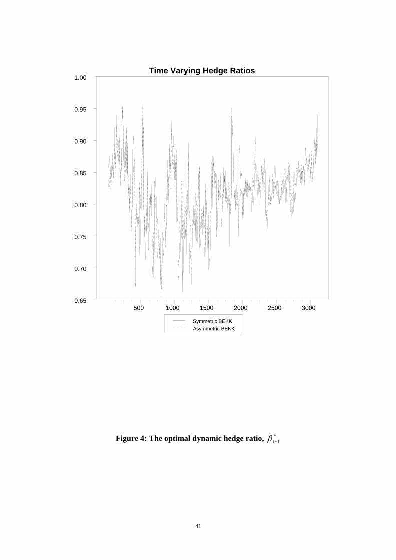
Figure 4 graphs the time varying hedge ratio from the symmetric and

asymmetric MGARCH models. The optimal hedge ratio is never greater than

0.9586 futures contracts per index contract, with an average value of 0.8177

futures contracts sold per long index contract. The variance of the estimated

optimal hedge ratio is 0.0019. Moreover the optimal hedge ratio series

obtained through the estimation of the asymmetric GARCH model appears

stationary. An ADF test (see, for example, Fuller, 1976) of the null hypothesis

*

1t ~I(1) was strongly rejected by the data (ADF=-5.7215, 5% Critical value

= -2.8630). The time varying hedge requires the sale (purchase) of fewer

futures contracts per long (short) index contract.4

The optimal hedge ratio *

1t may be linked to the arrival of news to

the market using (5) and the relevant futures price and covariance news impact

surfaces. Evaluating *

1t in the range 5,5, tj for j=futures, cash as

before gives us the response of the optimal hedge to news. Note that the

surface is drawn under the assumption that the portfolio is long the stock index

16

and the optimal hedge ratio is written in terms of the number of futures

contracts to sell. A negative optimal hedge ratio thus implies the purchase of

futures contracts. Figure 5 graphs the response of *

1t to news.

It is worth noting that *

1t responds far more dramatically to bad news

about the cash market index than to news about the future price. Negative

innovations in the cash price cause the optimal hedge ratio to increase in

magnitude towards 1. Large positive innovations in the cash price suggest a

negative hedge ratio. This might appear counter intuitive, however the surface

is drawn holding past information constant. The implication of the asymmetry

is that the hedge has very low value in bull market situations. In contrast, the

cointegrating hedge implies that the hedging surface is a plane at *

1t = =1.

One possible interpretation of the better performance of the dynamic strategies

over the naive hedge is that the dynamic hedge uses short run information,

while the cointegrating hedge is driven by long run considerations. The

performance evaluation in table 3 is in terms of one-day-ahead hedges. In the

next section we use a new criterion to judge hedging over various horizons,

including the one-day horizon.

5. Evaluating Hedging Effectiveness by Calculating Minimum Capital

Risk Requirements

Ensuring that banks hold sufficient capital to meet possible future

losses has been a topic of great import for regulators and risk managers in

recent years. A very popular approach involves the calculation of the

institution’s value at risk (VaR) inherent in its trading book positions. VaR is

an estimation of the probability of likely losses which might occur from

17

changes in market prices from a particular securities position, and the

minimum capital risk requirement (MCRR) is defined as the minimum amount

of capital required to absorb all but a pre-specified percentage of these

possible losses. We address an approach to the calculation of MCRRs which is

similar in spirit to the approach adopted in many Internal Risk Management

Models (IRMM), proposed by Hsieh (1993).5

Capital risk requirements are estimated for 1 day, 10 day, 30 day, 3

month and 6 month investment horizons by simulating the conditional

densities of price changes, using Efron’s (1982) bootstrapping methodology

based upon the multivariate GARCH(1,1) model presented in equations (7)

and (9), both with and without asymmetries, for comparison. The simulated

errors are generated by drawing randomly, with replacement, from the

standardised residuals and hence a path of future Yt ‘s can be generated,

using the estimates of , , , C0, A11, and B11 from the sample and multi-step

ahead forecasts of Ht.

A securities firm wishing to calculate the VaR of a portfolio containing

the cash and futures assets7 would have to simulate the price of the assets

when it initially opened the position. To calculate the appropriate capital risk

requirement, it would then have to estimate the maximum loss that the

position might experience over the proposed holding period.6 For example, by

tracking the daily value of a long cash and short futures position and recording

its lowest value over the sample period, the firm can report its maximum loss

for this particular simulated path of cash and futures prices. Repeating this

procedure for 20,000 simulated paths generates an empirical distribution of the

maximum loss. This maximum loss (Q) is given by:

18

Q = (x0 - x1) (12)

Where 0x is the initial value of the portfolio and x1 is the lowest simulated

value of the portfolio (for a long futures position) or the highest simulated

value (for a short futures position) over the holding period. We can express the

maximum loss as a proportion of the initial value of the portfolio as follows:

0

1

0

1x

x

x

Q (13)

In this case, since 0x is a constant, the distribution of Q will depend on the

distribution of 1x .

From expression (13), it can be seen that the distribution of 0x

Q will

depend on the distribution of 0

1

x

x. Hence, the first step is to find the 5

th

Quantile of

0

1

x

xLn :

Sd

mx

xLn

0

1

(14)

Where is the 5th

Quantile from a standard normal distribution, m is the

Mean of

0

1

x

xLn

and Sd is the Standard deviation of

0

1

x

xLn . Cross-

multiplying and taking the exponential,

x x Exponential Sd m1 0 [( ) ] (15)

therefore

Q x Exponential Sd m 0 1{ [( ) ]}

(16)

19

In this paper, we compare the MCRRs generated by the portfolios

constructed using the hedge ratios derived from the models described above.

The asymmetric multivariate GARCH model appears well specified and able

to capture the salient features of the data. Given this, we now determine what

would be an appropriate amount of capital to cover the cash and futures

portfolio derived from the hedge ratio as implied by the model. In particular,

we consider whether this portfolio minimises the need for capital, given that

all such capital is tied up in an unproductive and unprofitable fashion.

The estimated minimum capital risk requirements are presented in

tables 4 and 5 for each of the models, ignoring and allowing for asymmetries,

respectively, and are given in units of index points8. Panel A of Tables 4 and 5

present the MCRR for a short hedge (long cash, short futures). While Panel B

of the tables presents the results for a long hedge (long futures, short cash).

The most important feature of the results is that any type of hedge, even a

naïve hedge, is better than a naked exposure. Moreover, at short investment

horizons, there are large gains to be made by allowing the hedge to vary over

time. For example, the short hedge portfolio MCRR is 22.2 index points for a

naïve hedge, but only 11.8 for a Multivariate GARCH hedge. The long hedge

positions seem to be more risky overall over our out of sample period,

generating higher values at risk than the corresponding short hedges.

The gain from the use of an asymmetric model, as opposed to a

constrained symmetric model, which does not allow good and bad news to

effect returns differently, is large at short time horizons. For example, for the

symmetric time-varying short hedge, the portfolio MCRR is 11.8, while

modelling the asymmetries reduces this to 2.0. However, the benefit of these

20

more complex asymmetric and time-varying hedges, and moreover, the

benefits of hedging per se, are considerably reduced as the time horizon is

extended beyond one month. For example, the MCRR for a long hedge

calculated using asymmetric MGARCH is less than 10% of that using no

hedge at the one day horizon, but rises to more than 25% over a 6 month

hedging period. This result is in agreement with the findings of Lin et al.

(1994).

6. Conclusions

This paper sought to advance the extant literature in this field by

considering the impact of asymmetries on the hedging of stock index positions

using financial futures contracts9. We found that asymmetric models, which

allow positive and negative price innovations to affect volatility forecasts

differently, yielded improvements in forecast accuracy in sample, but not out

of sample, when evaluated using the traditional variance of realised returns

metric.

The paper also demonstrated how such hedging methodologies could

be evaluated in a modern risk management context, using a technique based

on the estimation of value at risk. Our primary finding was that allowing for

asymmetries led to considerably reduced portfolio risk at the shortest

forecasting horizons, and modest benefits when the duration of the hedge was

increased.

Our results have at least two important implications for those financial

market transactors who wish to reduce their exposure to risk using futures

contracts, and for further research in this area. First, hedge ratios which are

21

determined taking into account asymmetries in volatility are expected, in

general, to be more effective than those which do not. Second, since recent

changes in legislation in Europe have allowed market risk to be determined

using value at risk technologies under the second EC Capital Adequacy

Directive (CAD II), it is surely desirable for hedgers to measure the risk

inherent in their hedged portfolios in a similar fashion. Such procedures are

already now in widespread use in Europe as well as the US. The value at risk

approach is (or soon will be) used to assess the risk of the books of securities

firms as a whole. The use of traditional methods for assessing hedging

effectiveness, such as portfolio return variances, could be incompatible with,

and give very different results to, those based on value at risk methods.

22

Footnotes

* This paper was written while the second author was on study leave at the

ISMA Centre, Department of Economics, The University of Reading. The

development of this paper benefited from comments by the anonymous

referees and discussions with Salih Neftci, Simon Burke and Peter Summers.

The responsibility for any errors or omissions lies solely with the authors.

1 Note that we are not requiring at this stage that the hedge ratio, t-1, be time-

varying, but rather that it is determined using information to time t-1.

2 Since these contracts expire 4 times per year - March, June, September and

December - to obtain a continuous time series we use the closest to maturity

contract unless the next closest has greater volume, in which case we switch to

this contract.

3 The reason for this is that the minimum price movement (known as tick) for

the futures contract is £12.50 i.e. a change of 0.5 in the index.

4 Although, of course, a time-varying hedge may result in considerably

increased transactions costs in the likely event that such a hedge requires daily

adjustments of the futures position. We therefore cannot state categorically

that the time-varying hedge would be cheaper.

5 See also Brooks et al. (2000) for a more detailed description of this

methodology and issues in its implementation.

23

6 See Dimson and Marsh (1997) for a discussion of a number of potential

issues which a financial institution may face when calculating appropriate

levels of capital for multiple positions during periods of stress.

7 The current BIS rules state that the MCRR should be the higher of the: (i)

average MCRR over the previous 60 days or (ii) the previous trading days’

MCRR.

8 See section 3 above. Although Hsieh (1993) and Brooks et al. (2000)

measure MCRRs as a proportion of the initial value of the position, this is not

sensible in our case since by definition an appropriately hedged portfolio will

have a zero value.

9 Although the methodology could, of course, be equally applied to hedging a

position in any financial asset using futures contracts.

24

References

Baillie, R.T. and Myers, R.J. 1991. Bivariate GARCH estimation of the

optimal commodity futures hedge. Journal of Applied Econometrics 6

(April): 109-124.

Bollerslev, T., Engle, R.F. and Wooldridge, J.M. 1988. A capital asset pricing

model with time-varying covariances. Journal of Political Economy 96

(February): 116-31.

Brooks, C., Clare, A.D. and Persand, G. 2000 A word of caution on

calculating market-based capital risk requirements. Journal of Banking

and Finance forthcoming.

Cechetti, S.G., Cumby, R.E., Figlewski, S. 1988. Estimation of optimal futures

hedge. Review of Economics and Statistics 70 (November): 623-630.

Dimson, E. and P. Marsh 1997. Stress tests of capital requirements. Journal of

Banking and Finance. 21 (July): 1515-1546.

Efron, B. 1982. The Jackknife, the Bootstrap, and Other Resampling Plans,

Philadelphia, PA: Society for Industrial and Applied Mathematics.

Engle, R.F. and Granger, C.W.J. 1987. Cointegration and error correction:

representation, estimation and testing. Econometrica 55 (March): 251-

76.

25

Engle, R.F. and Ng, V. 1993. Measuring and testing the impact of news on

volatility. Journal of Finance, 48 (December): 1749-1778.

Engle, R.F. and Kroner, K. 1995. Multivariate simultaneous generalised

ARCH. Econometric Theory, 11 (March), 122-150.

Fuller, W.A. 1976. Introduction to Statistical Time Series Wiley, N.Y.

Garcia, P., Roh, J-S, and Leuthold, R.M. 1995. Simultaneously determined,

time-varying hedge ratios in the soybean complex. Applied Economics

27 (November): 1127-1134.

Ghosh, A. 1993. Cointegration and error correction models: Intertemporal

causality between index and futures prices. Journal of Futures Markets

13 (April): 193-198.

Glosten, L.R., Jagannathan, R. and Runkle, D.E. 1993. On the relation

between the expected value and the volatility of the nominal excess

return on stocks. The Journal of Finance 48 (December): 1779-1801.

Hodgson, A. and Okunev, J. 1992. An alternative approach for determining

hedge ratios for futures contracts. Journal of Business Finance and

Accounting 19 (January): 211-224

26

Hsieh, D.A. 1993. Implications of non-linear dynamics for financial risk

management. Journal of Financial and Quantitative Analysis 28

(March): 41-64.

Johansen, S. 1988. Statistical analysis of cointegration vectors Journal of

Economic Dynamics and Control 12, 231-254.

Kroner, K.F., and Ng, V.K. 1998. Modelling asymmetric co-movements of

asset returns. Review of Financial Studies, 11 (Winter): 817-844.

Kroner, K.F. and Sultan, J. 1991. Exchange rate volatility and time-varying

hedge ratios. In Rhee, S.G. and Chang, R.P. (eds.) Pacific Basin

Capital Markets Research. Elsevier, North Holland.

Lien, D. and Luo, X. 1993. Estimating multiperiod hedge ratios in

cointegrated markets. Journal of Futures Markets 13 (December): 909-

920.

Lin, J.W., Najand, M., and Yung, K. 1994. Hedging with currency futures:

OLS versus GARCH. Journal of Multinational Financial Management

4 (January): 45-67.

Myers, R.T. and Thompson, S.R. 1989. Generalised optimal hedge ratio

estimation. American Journal of Agricultural Economics 71

(November): 858-867.

27

Park, T.H. and Switzer, L.N. 1995. Bivariate GARCH estimation of the

optimal hedge ratios for stock index futures: A note. Journal of

Futures Markets 15 (February): 61-67.

Strong, R.A. and Dickinson, A. 1994. Forecasting better hedge ratios.

Financial Analysts Journal. 50 (January-February): 70-72.

Sutcliffe, C. 1997. Stock Index Futures: Theories and International Evidence.

Second Edition, Thompson Business Press, London.

28

Table 1: Summary Statistics and Cointegration Tests

Panel A: Summary Statistics for the data

ADF() ADF

Ft -1.7028 1.9982

Ct -1.0082 2.2269

Series Mean Variance Skewness Excess

Kurtosis

ΔFt 0.0392 1.1424 -1.6081 25.3160

ΔCt 0.0389 0.8286 -1.6602 25.6852

29

Panel B: Engle Granger Cointegration Tests

Ft as dependent variable

0 1 ADF() ADF

-0.0327

(0.0039)

1.0031

(0.0005)

-8.3846 -8.3859

Ct as dependent variable

0 1 ADF() ADF

0.0386

(0.0039)

0.9961

(0.0005)

-8.4026 -8.4039

Panel C: Johansen Cointegration Tests

M T

r = 0 91.75 92.58

r = 1 0.83 0.83

Likelihood Ratio Tests

H0: ’=[-1,1] H0: =[1,0] H0:’=[-1,1] | =[1,0]

5.51

[0.06]

4.4800

[0.0300]

0.06900

[0.4000]

30

Table 2: Estimates of the Multivariate Asymmetric GARCH Model

Conditional Mean Equations

tC

tF

t

C

F

C

Ci

C

Fi

F

Ci

F

Fi

i

C

F

t

t

t

ttit

i

it

P

FY

vYY

,

,

)(

,

)(

,

)(

,

)(

,

1

4

1

;;;;

)0061.0(

0257.0

)0053.0(

0759.0

)0072.0(

0225.0

)0060.0(

0078.0

1

0092.0

0238.0

0080.0

0272.0

)0110.0(

1399.0

)0089.0(

1499.0

2

0117.0

0293.0

0114.0

0352.0

0149.0

1083.0

0111.0

1225.0

3

0232.0

0032.0

0182.0

0141.0

0256.0

0084.0

0227.0

0699.0

4

0050.0

0523.0

0057.0

0518.0

0142.0

1719.0

0195.0

1636.0

2454.0

0606.6

31

Table 2 Continued:

Estimates of the Multivariate Asymmetric GARCH Model

Residual Diagnostics

Mean Variance Skewness Excess

Kurtosis

Q(10) Q2(10)

tF , -0.0023 1.0790 -0.9077

[0.0000]

12.7237

[0.0000]

13.3361

[0.2055]

2.1991

[0.9946]

tC , -0.0079 1.0438 0.4578

[0.0000]

5.9459

[0.0000]

12.0461

[0.2820]

7.6730

[0.6607]

Notes: Standard errors displayed as (.). Marginal significance levels displayed

as [.]. Q(10) and Q2(10) are are Ljung_Box tests for tenth order serial

correlation in 2

,, and tjtj zz respectively for j = F,C.

32

Table 2 Continued: Estimates of the Multivariate Asymmetric GARCH

Model

Conditional Variance-Covariance Structure

)0,min(

)0,min(;

1,

1,

1

1,

1,

1

*

11

'

11

*'

11

*

111

*'

11

*

11

'

11

*'

11

*

0

*'

0

tC

tF

t

tC

tF

t

tttttt DDBHBAACCH

)0036.0(

0131.00

)0151.0(

1488.0

)0184.0(

1680.0

*

0C

)0072.0(

9633.0

0080.0

0217.0

)0067.0(

0031.0

)0077.0(

9785.0

*

11B

)0239.0(

2144.0

0289.0

0611.0

)00170(

0305.0

)0208.0(

1198.0

*

11A

)0892.0(

2576.0

1048.0

2172.0

)0717.0(

3528.0

)0885.0(

3685.0

*

11D

H0:ij=0 for i,j=1,2 30.7106

[0.0000]

33

Table 3: Portfolio Returns

In Sample

Unhedged

= 0

Naïve Hedge

= -1

(C.I. HEDGE)

Symmetric

Time Varying

Hedge

tF

tFC

th

h

,

,

Asymmetric

Time Varying

Hedge

tF

tFC

th

h

,

,

Return 0.0389

{2.3713}

-0.0003

{-0.0351}

0.0061

{0.9562}

0.0060

{0.9580}

Variance 0.8286 0.1718 0.1240 0.1211

Out of Sample

Unhedged

= 0

Naïve Hedge

= -1

(C.I. HEDGE)

Symmetric

Time Varying

Hedge

tF

tFC

th

h

,

,

Asymmetric

Time Varying

Hedge

tF

tFC

th

h

,

,

Return 0.0819

{1.4958}

-0.0004

{0.0216}

0.0120

{0.7761}

0.0140

{0.9083}

Variance 1.4972 0.1696 0.1186 0.1188

Notes: t-Ratios displayed as {.}

34

Table 4: MCRR Estimates - Symmetric Hedging Models

Panel A: Long Cash and Short Futures

Days Unhedged Naïve Hedge Time-Varying

Hedge

1

27.851 22.175 11.763

10

211.210 99.819 96.308

20

234.215 197.217 124.214

30

358.872 238.632 167.297

60

411.058 425.661 245.312

90

513.368 499.756 293.263

180

651.402 569.952 378.451

35

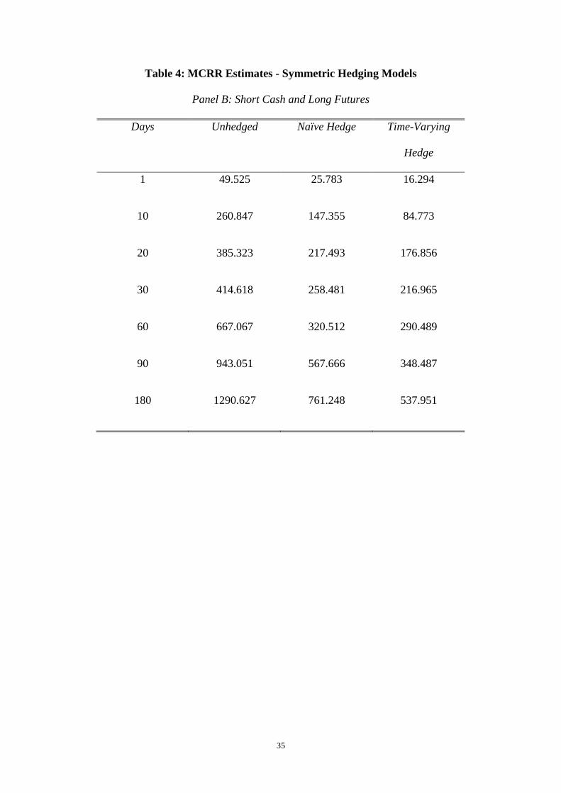
Table 4: MCRR Estimates - Symmetric Hedging Models

Panel B: Short Cash and Long Futures

Days Unhedged Naïve Hedge Time-Varying

Hedge

1

49.525 25.783 16.294

10

260.847 147.355 84.773

20

385.323 217.493 176.856

30

414.618 258.481 216.965

60

667.067 320.512 290.489

90

943.051 567.666 348.487

180

1290.627 761.248 537.951

36

Table 5: MCRR Estimates - Asymmetric Hedging Models

Panel A: Long Cash and Short Futures

Days Unhedged Naïve Hedge Time-Varying

Hedge

1

20.792 2.356 2.003

10

196.812 83.475 74.268

20

237.567 182.852 96.776

30

370.988 228.123 155.325

60

416.221 416.632 229.875

90

529.219 484.566 292.852

180

746.852 549.633 354.685

37

Table 5: MCRR Estimates - Asymmetric Hedging Models

Panel B: Short Cash and Long Futures

Days Unhedged Naïve Hedge Time-Varying

Hedge

1

46.852 8.511 3.321

10

228.562 120.256 83.523

20

415.785 176.118 105.963

30

507.952 213.963 153.523

60

717.633 315.784 221.541

90

1004.159 644.935 273.965

180

1462.774 743.226 381.522

38

Figure 1: News Impact Surface for Futures Market Volatility

39

Figure 2: News Impact Surface for Cash Market Volatility

40

Figure 3: Covariance News Impact Surface

41

Figure 4: The optimal dynamic hedge ratio, *

1t

Symmetric BEKK

Asymmetric BEKK

Time Varying Hedge Ratios

500 1000 1500 2000 2500 30000.65

0.70

0.75

0.80

0.85

0.90

0.95

1.00

42

Figure 5: Hedging Surface: The response of *

t to News