Sveriges lantbruksuniversitet Fakulteten för veterinärmedicin och husdjursvetenskap Swedish University of Agricultural Sciences Faculty of Veterinary Medicine and Animal Science

The effect of different starch levels on oxygen

consumption and nitrogen excretion of

Eurasian perch (Perca fluviatilis)

Rouzbeh Keihani

Examensarbete / SLU, Institutionen för husdjurens utfodring och vård, 407

Uppsala 2012 Degree project / Swedish University of Agricultural Sciences, Department of Animal Nutrition and Management, 407

Examensarbete, 30 hp Masterarbete Husdjursvetenskap

Degree project, 30 hp Master thesis Animal Science

Sveriges lantbruksuniversitet

Fakulteten för veterinärmedicin och husdjursvetenskap

Institutionen för husdjurens utfodring och vård Swedish University of Agricultural Sciences Faculty of Veterinary Medicine and Animal Science Department of Animal Nutrition and Management

The effect of different starch levels on oxygen consumption and nitrogen excretion of Eurasian perch (Perca fluviatilis) Rouzbeh Keihani Handledare:

Supervisor: Torbjörn Lundh

Bitr. handledare:

Assistant supervisor:

Examinator:

Examiner: Jan Erik Lindberg

Omfattning:

Extent: 30 hp

Kurstitel:

Course title: Degree project

Kurskod:

Course code: EX0551

Program:

Programme: Animal Science – Master’s Programme

Nivå:

Level: Advanced A2E

Utgivningsort:

Place of publication: Uppsala

Utgivningsår:

Year of publication: 2013

Serienamn, delnr: Examensarbete / Sveriges lantbruksuniversitet, Institutionen för husdjurens utfodring och vård, 407

Series name, part No: On-line publicering: On-line published: http://epsilon.slu.se Nyckelord: Key words: Starch, oxygen consumption, nitrogen excretion, Eurasian perch (Perca fluviatilis),

respirometry

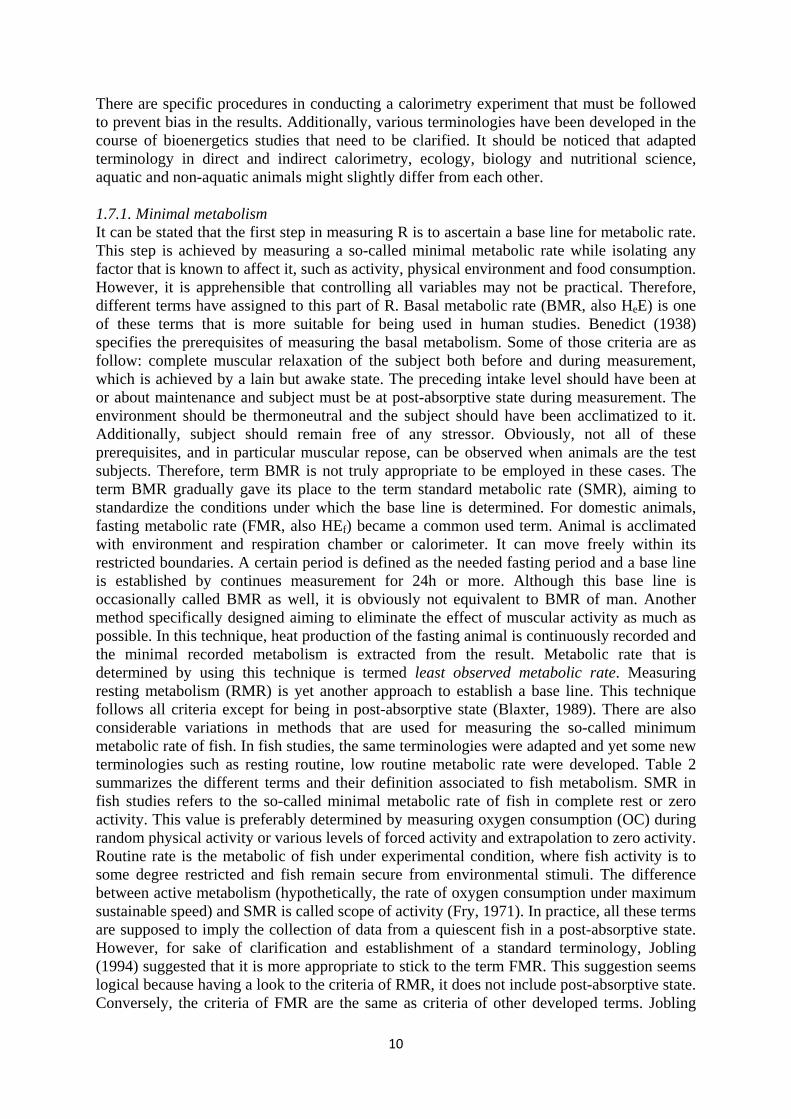
Contents Abstract .......................................................................................................................................... 1

1.Introduction ................................................................................................................................ 2

1.1. Background .......................................................................................................................... 2

1.2. Introduction of new fish species for farming in Europe ....................................................... 4

1.3. Fish as feed in aquaculture ................................................................................................... 4

1.4. Fish meal and fish oil alternatives ........................................................................................ 6

1.6. Energy loss as heat (R) ............................................................................................................ 7

1.7. Components of R: how to perform an indirect calorimetry experiment .............................. 9

1.7.1. Minimal metabolism .................................................................................................... 10

1.7.2. Feeding metabolism (RF) ............................................................................................. 11

1.8. A short review of different respirometers .......................................................................... 13

The aim of this thesis ............................................................................................................... 14

2. Materials and methods ........................................................................................................... 14

2.1. Experimental fish and acclimation ..................................................................................... 14

2.2. Facilities and measuring devices: ....................................................................................... 14

2.2.1. Respirometer ................................................................................................................ 14

2.2.2. Measurement devices ................................................................................................... 15

2.3. Experimental feed .............................................................................................................. 15

2.4. Experimental procedures .................................................................................................... 17

2.5. Calculation and statistical procedure .................................................................................. 17

3. Results ...................................................................................................................................... 18

3.1. Oxygen consumption .......................................................................................................... 18

3.2. Ammonia excretion ............................................................................................................ 20

4. Discussion ............................................................................................................................. 22

5. Conclusion ............................................................................................................................ 25

References ..................................................................................................................................... 26

Appendix ....................................................................................................................................... 33

1

Abstract Aquaculture is one of the fastest-growing and valuable industries nowadays. Because fish meal and fish oil are the major components of fish diets, there is growing concern that the rapid growth of this industry will lead to either fish meal scarcity or the depletion of marine fish population. Fish utilize parts of protein and oil in their diets only as sources of energy. Therefore, parts of the aforementioned substrates are replaceable by other sources of energy such as digestible carbohydrates. Nonetheless, fish have limited ability to assimilate carbohydras and consequently, species-based research is needed for determining the appropriate level of carbohydrates in fish diets. An indirect calorimetry study was performed on Eurasian perch using diets with four different levels of raw wheat starch (0%, 10%, 20% and 30%). We measured oxygen (OC) consumption and ammonia excretion (AE) in response to different carbohydrate levels. The OC was not significantly different between treatments but the results showed numerically decreasing values (1.62- 1.15 mg min-1 kg-1BW) with increased inclusion of starch in the diet. The fish consumed more oxygen on the second experimental days compared with the first experimental days (P=0.001).The ammonia excretion was highest in 0% and 30% Starch diets and lowest in fish fed 10% Starch, which indicated that 10% inclusion caused a protein sparing effect. Based on the results of our experiment, the inclusion of 10% raw starch in the diet of Eurasian perch appears to be beneficial and unproblematic.

2

1. Introduction

1.1. Background Aquaculture with an average annual growth of 6.1 percent from 2001 to 2009 is one of the fastest-growing and valuable industries nowadays. One hundred ninety countries worldwide are rearing over 541 aquatic species including 327 finfishes, 102 mollusks, 62 crustaceans, 6 amphibians and reptiles, 9 aquatic invertebrates and 35 algae species at present time. China, India, and Vietnam with 62.5, 6.8, and 4.6 percent of the total world aquaculture production, respectively were the largest aquaculture producers of the world in 2009 (FAO, 2009). At the same time, the European Union (EU) aquaculture production accounted for 2.3 % of the total world aquaculture products. Within EU, the largest aquaculture producer was Spain (20.6%), and it was followed by France (18.2%) and the United Kingdom (15.1%). Nonetheless, in term of production value, France took the first place with 21.5% of total EU trade value, and it was followed by the United Kingdom (16.7%), Italy (14.6%), Greece (12.2%), and Spain (12.2%). Among Scandinavian countries, Norway came first with total aquaculture production of about 960 thousand tons in 2009, followed by Denmark (40 thousand tons)and Sweden (8.5 thousand tones) (CFP, 2012). Carps were the most cultured species in 2009, and accounted for 40% of total global aquaculture production volume. White leg shrimp, Atlantic salmon, grass carp, silver carp and common carp were the world’s most profitable products (FAO, 2009). The ongoing aquaculture systems can be categorized into three groups of open, semi-closed, and closed systems. Additionally, production may take place as monoculture or polyculture/ integrated system. Open system is probably the oldest production system, where production occurs in natural bodies of water. Floats, trays, and rafts are commonly used for bivalve production and cages or net pens for finfish and sometimes crustaceans (Tidwell, 2012). Cage system is predominately used for culturing marine fish in Europe. The European Commission policy urges to install any new extension of marine aquaculture preferably 2 km away from the shores into open oceans. The main arguments are the adverse impact of inshore production on environment and the lack of inshore space. Additionally, the conflict and competition between inshore sites and tourist industry move ahead occasionally. Remote sites generally allow large-scale production without disquiet about space and resources. The future of offshore system is still unclear. Production must be run on a large scale to be economically viable, which practically leads to high initial capital costs. The same reason limits the possibility of research on these systems. Difficulties with feeding, harvesting, routine maintenance of wear and tear, possibility of fish loss, and dangerous working environment are other barriers that make the system less appealing (Sturrock, 2008). Semi closed systems consist of two forms, namely pond and raceway systems. Because of higher management and supervision abilities, the capacity of production is most often greater than open systems. Instead, the system demands higher inputs and water quality and disease could be major problems (Fornshell et al, 2012; Tidwell, 2012). Semi closed systems in most cases consumes high volume of water. Generally, two types of water usage are contemplated in aquaculture. One type is the total water usage determined by the sum of all inflows. Another type is consumptive usage, which represents the amount of water that disappears and no more is available for other purposes. Total water usage can vary from less than 2 m3 kg-1 in a fish extensive culture without water exchange to 80 m3 kg-1 for marine shrimp production pond. To have a comparative view, total water usage in trout race way is about 100 m3 kg-1 product, 3 to 10 m3 kg-1 for semi intensive pond production and 0.1 m3 kg-1 for recirculation system. The consumptive usage is the greatest in pond production. The wide exposed

3

surfaces of ponds lead to significant water loss through evaporation (1 to 5 vs. 0.1 m3 kg-1 for race way and recirculation). According to FAO (2012), the average annual growth of freshwater aquaculture production from 2000 to 2010 was 7.2%. Considering the limited availability of fresh waters on the earth, it is reasonable to infer that such consumption is a threat to the availability of freshwaters in the future (Bostock et al., 2010). The mentioned concerns encourage using alternative systems that can deploy water with higher efficiency. Recirculating aquaculture systems (RAS) gives the ability to treat water for reusing or before discharging it. The proportion of water that is treated and reused may vary from 50% to 99.9%, creating semi to full recirculation systems. Overall, the advantages of RAS are decreased land and water usage, better water quality control, better management of animal requirements, waste management, lower environmental impacts, and higher biosecurity. The main limitations of the system are perhaps high investment and operation costs, and lack of knowledge for targeted species. RAS is currently used at different levels of production in some EU countries (appendix, Table 1A) (Sturrock et al., 2008). “It’s very rewarding to see what some considered a “strange idea” six years ago, as a research priority; now, After several years of preaching in the desert, it seems we are coming close to the oasis!” (Chopin, 2006). What it is mainly known as integrated Aquaculture (IA) has a long history of practice. Various methods and species, particularly in Asia, have been introduced to this system. Nonetheless, a new style of this system has recently attracted attentions. This type of integrated system, which can be regarded as a newly emerged system, is sometimes named Integrated Multi-Trophic Aquaculture (IMTA). Terminology was developed to distinguish IMTA from polyculture and Integrated Agriculture-Aquaculture (IAA). According to Chopin (2006), polyculture can be referred to any production system that is combined species (three finfish for example), whereas production is exclusively termed IMTA when the combined species are from different trophic levels and able to use each other waste metabolites. IMTA can be highly flexible and adaptable to different environments. A simplified model of IMTA can include a fed aquaculture (finfish/ shrimp), an organic extractive species (e.g. a shellfish) to use particulate organic matters (POM), and an inorganic extractive species (e.g. seaweed) to utilize dissolved inorganic nutrients (DIN) (Figure1).

Figure 1 Schematic diagram of an integrated multi-trophic aquaculture (IMTA) operation (adapted from Chopin, 2006) Research is still in initial stages, but it has been paid remarkable attention recently. In Canada, Bay of Fundy, research showed promising results. Cultivating kelp and mussel close to salmon sites led to increased production of 46% and 50% for kelp and mussel, respectively. Study in Scotland indicates that approximately 30% of wasted nutrient from a

4

500 tons salmon farm is recovered if production is integrated by 1 hectare of alga (FAO, 2009b).

1.2. Introduction of new fish species for farming in Europe All EU countries encourage employing new species based on common fishery policy’s recommendations (see Table 2A of appendix for 10 dominant produced species in EU). Over 40 new species have been introduced for commercial production in Europe during the last 10 year. Among them, Bluefin tuna, cod, and various sea breams were the most successful introduced species. The emerged species in Sweden are mainly arctic charr, perch and pikeperch (Sturrock et al., 2008). Ministry of Agriculture (Swedish Parliament 2007), nonetheless, listed catfish, cod, and bass as species with the best development potential (review of the EU aquaculture sector, 2009). As perch was the species that we used in our experiment, some information about this fish would be pertinent to our topic. Eurasian perch (Perca fluviatilis) is a carnivore cool water fish with shoaling temperament. This fish is widely distributed in Eurasia and has been introduced to Australia, New Zealand, and South Africa as well. The family Perca contains two other species, namely Perca flavescence (yellow perch), which lives in North America, and schrenki Kessler (Balkhash perch) which is only found in the Balkhash Lake in Kazakhstan. Both yellow perch and Eurasian perch have been identified as candidates for aquaculture. For both fish, commercial landing has decreased in recent years due to legalization for conserving them. Currently, capture cannot keep pace with market demands and it has been associated with interest in commercial production of these fish (Craig, 2000). The biological characteristics make these fish suitable candidates for aquaculture. They are considered thriven species with high adaptability to new environment, high fertility rate, low spawning requirement, and rapid expansion. The life length varies from six month to 21 years. These fish have an upper temperature limit of around 29- 31 ̊ C and can endure wide ranges of environment conditions. A low temperature apparently more affects their food consumption and reproductive function more than their survivability. The physiological optimum temperature is around 22-24 ̊ C. Protein requirements of perch and salmonids are generally considered to be alike (40-50% CP for maximum growth), yet the lipid contents of salmonids diets appear to be higher (may be twice more) than perch requirements (Craig, 2000). Percids are not very active or energetic species and tolerate crowding positively. Densities as high as 50-120 kg m3 are achievable by RAS if oxygen level is kept above 4-5 mg l-1. They exhibit considerable resistance to low levels of oxygen. The reported lethal concentrations for Eurasian perch at 20-26 ˚C is 2.25 mg l-1 and 1.1-1.3 mg l-1 at 16 ̊ C. It has been reported that yellow perch beneath the ice of northern lakes of North America tolerates oxygen concentration as low as 0.25 mg l-1 at 2.5-4 ̊ C, although ice nosing under this condition was observed (Craig, 2000).

1.3. Fish as feed in aquaculture There is growing concern that the rapid development of aquaculture will increase the need for fish meal to the extent that either there will be not enough fish meal available or it will lead to the depletion of wild fish population. Therefore, debates concerning fish meal are founded on two pivotal presuppositions. First, fish meal scarcity limits the growth of aquaculture in the future. Second, high demands of fish meal leads to overfishing and depletion of wild fish. To appraise the feasibility of these assertions, we need to have a glimpse into fish meal and oil consumption by aquaculture. International fish meal and fish oil organization (IFFO) publishes a graph (Figure 2) in response to supporters of these assertions, illustrating fish

5

meal and oil consumptions under the realm of developing aquaculture. Despite the growth of aquaculture industry and elevated feed usage, the consumption of fish meal and fish oil has remained constant since 2004 and 2000, respectively. IFFO concludes that fish meal neither is a limiting factor for the expansion of aquaculture nor causes pressure on marine fish stocks. The discrepancy between aquaculture growth and fish meal consumption can be explained by several reasons. One effective reason is high price of fish meal. Another reason is costumer tendency for more sustainable products. Additionally, improved nutritional knowledge and feed conversion rate (FCR, see table 3A in appendix for current FCR) have contributed to further reduction of fish meal usage (Tacon & Metian 2008; Jackson, 2009).

Figure 2 Growth of aquaculture and fed aquaculture and use of fish meal and fish oil in aquaculture 2000-2008 (in millions of tons). Source: IFFO, 2010 Although the issue of fish meal scarcity is not currently envisaged as an impeding factor for aquaculture growth, some uncertainties about far future exist. Aquafeed industry is operating in parallel with other industries such as pork, poultry, beef, and human food industries, all competing on common resources. The aquaculture sector is the major consumer of produced fish meal and fish oil (63 and 81% in 2009, respectively; see also Figure 1A in appendix.) (Bostock et al., 2010; IFFO, 2011). The excessive dependency of aquaculture on fish meal and fish oil makes the industry highly vulnerable to any aggravation of feed price. Since 2005, the price of main feed ingredients including soybean meal, fish meal, corn, and wheat augmented by 67, 55, 124 and 130 %, respectively. Likewise, the price of main food oils rose by 250% from 2005 to 2009 (see Figure 2A in appendix). Furthermore, there is decisive evidence that fluctuations in fish meal and oil production cause ample instability in the entire feed ingredients due to extreme dependency of aquaculture to these products (Rana et al., 2009). On the other hand, according to estimates by FAO (2012), production should increase at least by 23 million tones until 2020 if the present per capita level of consumption is supposed to be maintained. Taking into account that there is no more room for increasing wild fish capture (assessments indicate that 52% of marine stocks are fully exploited and 29.9% are overexploited; FAO, 2012), this extra amount should inevitably emanate from aquaculture. Considering all the above-mentioned points as well as making allowances for the fact that marine fish population fluctuate wildly even in the absence of fishing (Gulland, 1982; Werner & Quinlan, 2002), it can be intuitively plausible to make a pre-cautionary management to reduce dependency of aquaculture to fish by-products.

6

1.4. Fish meal and fish oil alternatives Nowadays, it is comprehensively admitted that instability of global weather is increasing. Hostile conditions for production of fish by-products along with an air of uncertainty about the global market of feed ingredients have impelled specialists to develop strategies for dealing with unfortunate market-driven problems. One of the ongoing strategies is unveiling alternative energy and protein sources to replace fish meal and oil. By inference, one may surmise that studies on alternatives focus upon three main fields. 1. Feasibility studies: Testing new ingredients and scrutinizing the likely advantages and

disadvantages. 2. Allowance studies: Determining the highest possible inclusion level of an alternative

ingredient in different species. 3. Ameliorative studies: Investigating the potentials for increasing maximum allowance by

means of modification of ingredients, processing methods, etc. to overcome limiting factors.

Since now, a wide variety of alternatives has been tested by different degrees of success. Based on a general classification, fish meal/oil alternatives can be divided into two groups of plant-driven ingredients and animal-driven ingredients (Gatlin et al., 2007; Ferouz et al., 2012). Gatlin et al., (2007) specify certain characteristics for a viable plant-driven alternative. The candidate alternatives should have certain properties consisting of high accessibility, reasonable price, and allowing for easy handling, shipping, and usage. Nutritionally, an alternative should fit fish ability to digest it (i.e. low levels of fiber, starch, non-soluble carbohydrates, and anti-nutrients) and fulfill fish requirement for optimum growth and health. Some of alternatives are widely used in aquafeeds at present time. Soybean, as a typical example, is considered an economically viable substitute for fish meal in certain forms. It may incorporate into aquafeeds in forms of full-fat soybean, soy flour, soybean meal (SBM), soy protein concentrate (SPC) or soy protein isolate (SPI). Inclusion of SBM usually entitles adding some essential amino acids (EAA), chiefly lysine, methionine, and threonine. Additionally, mineral (phosphorus largely occurs in form of phytic acid) and vitamin supplements are recommended. It is worth mentioning that amino acid taurine is practically absent in all plant products. It has been suggested that this amino acid can be limiting in plant-based diets, even in species such as rainbow trout, which has ability to synthesize it (Gatlin et al., 2007). The presence of undesirable carbohydrates is yet another limiting factor in using plant seeds. Non-soluble carbohydrates such as raffinose and stachyose are not digestible for fish due to lack of α-galactosidases. Both compounds have been reported to cause increased chime viscosity, enteritis, reduced nutrient uptake and growth performance for salmonids species (Gatlin et al, 2007). There is considerable variation in fish ability to assimilate digestible/soluble carbohydrates as well. The recommended dietary level of digestible carbohydrate for cold-water carnivore and warm water omnivore fish species are up to 20% and 40%, respectively (Wilson, 1990). The difference between cold and warm water fish can be related to higher intestinal amylase activity of warm water species. It has been observed that processed (gelatinized) starch is digested with higher efficiency than native (raw) starch. Additionally, high level of dietary starch regardless of source and processing has been reported to cause dramatic reduction in starch digestibility. Again, the reason might be due to inadequate enzyme production and enzyme saturation (Stone, 2003). Apart from digestibility, fish shows some disability to clear the blood glucose at the same rate of mammals. It has

7

been reported that both high amount of digestible carbohydrate and oral administration of glucose lead to a persistent hyperglycemia in some species. A hyperglycemic fish excretes glucose in urine and through the gills (Bureau et al., 2002). Therefore, the fact that a diet is digested and absorbed cannot signify that all metabolisable energy in the given diet will be available for utilization.

1.5. Carbohydrate as a source of energy: How to evaluate

Apart from the nutritional importance of protein and oil macronutrients in synthesizing or turnover of cells and tissues, fish use both and in particular oil as energy sources. The outcome of protein catabolism as an energy source is increased amount of nitrogen excretion, which is counted as protein wastage. In addition, oil ingredients are relatively expensive sources of energy in comparison to carbohydrate (see Figure 2A of appendix). The portions of protein and oil in the diet that merely convert to energy are theoretically replaceable with digestible carbohydrates such as starch. However, as mentioned earlier, fish show limited ability to digest and utilize carbohydrates. Additionally, the variations in digestion and utilization of carbohydrate impel species-based investigation to determine the appropriate level of carbohydrate inclusion in their diets. At the same time, it can be of interest to study whether or not there is any traceable response in metabolic rate of the animal along with diet alteration. When it comes to evaluation of a diet or a new ingredient in a diet, it is the concept of energetic that often comes in focus. A balance sheet of an energy budget needs to include energy inputs and energy outputs. Additionally, it should be considered that a live organism is thermodynamically an open system, which exchanges both energy and matter with environment. In the case of non-chlorophyllous organism, the input is mainly in form of matter while the outputs are in both forms of matter and energy (Wiegert, 1968; Lucas, 1992). Based on this knowledge, the matter-energy exchange can be elucidated in a standard/basic energetic equation, C=P+R+E, where C stands for energy of the consumed food, P the energy in the growth materials (production), R the loss of energy in form of heat (R stands for respiration), and E is lost as waste products (excretory products). In addition, it is assume that work done by the animal on the environment, and vice versa, is small and ignorable. Theoretically, all parameters of the basic equation should be measured concurrently to give a complete accurate energy sheet. Practically, however, innumerable problems appear that make such target hard to accomplish. Every element of the equation can be subdivided further. In this paper, we focus on the factors that are relevant to our research, including parts of E and R. E as waste products can be subdivided to three components of energy lost in feces (F), energy lost in nitrogenous excretory products (U), and, when it is applicable, secretory products such as mucus. R can be also partitioned to standard metabolism (RS), routine metabolism (RR), feeding metabolism (RF), and active metabolism (RA) (Brafield, 1985; Calow, 1985).

1.6. Energy loss as heat (R) After absorption, nutrients are either catabolized or stored as new tissues. Catabolism of nutrients in the body is accompanied by release of some non-captured energy that exhibits itself as heat. One of the methods that are used to quantify heat loss is calorimetry. This method notably allows nutritionist to determine heat production in a relatively short-time experiment. Calorimetry can be conducted by two methods, namely direct and indirect calorimetry (Bureau et al, 2002). In the direct method, the heat production of animals is

8

determined by measuring the change in animals’ surrounding temperature. Despite the successful usage of this method in mammals, there are some hesitations in employing it for aquatic animals. High heat capacity of water, need for precise thermometers, and a possible change in temperature due to oxygenation and water exchange make it difficult to verify the results of such experiments (Brett& Groves, 1979; Lucas, 1992; Bureau et al, 2002). Therefore, indirect calorimetry is the most widely used method for calculation of heat loss in aquatic animals. This method can be carried out using two approaches. One approach is to measure only oxygen consumption during a specific time. The second approach is to expand the measurements and include carbon dioxide and nitrogen excretion as well. The first approach is more common than the second one due to difficulties in spontaneous measuring of O2, NH3, and CO2 (Brafield, 1985). To have the results of indirect calorimetry in form of energy, the total measured parameters must be multiplied by an appropriate coefficient. In the case of oxygen, the coefficient is called oxycalorific or heat coefficient of oxygen (Qox) and the results normally express in joules or calories. The value of Qox varies based on the respired substrate. To have the results of indirect calorimetry in form of energy, the total measured parameters must be multiplied by an appropriate coefficient. In the case of oxygen, the coefficient is called oxycalorific (Qox) and the results normally express in joules or calories. The value of Qox varies based on respired substrate. For example, the combustion of one mole carbohydrate leads to release of 2833 kJ energy, and combustion of one mole glucose consumes six moles (192 g) oxygen. Therefore, the Qox of carbohydrates are approximately 2833/192=14.76 J mg-1 oxygen. For protein, the calculation is based on 100g of a natural protein containing 53 % carbon (53/12 {atomic mass of carbon} ≈ 4.42 moles carbon), 7 % hydrogen (7/1=7.00 moles hydrogen), 23 % oxygen (23/16≈ 1.44 moles oxygen), and 16 % nitrogen (16/14≈ 1.14 moles nitrogen). Accordingly, as it suggested by Brafield and Llewellyn (1982), equation of protein oxidation when the excretory product is ammonia can be written as follow: (4.42 C, 7.00 H, 1.44 O, 1.14 N) + 4.6 O2 1.14 NH3 + 4.42 CO2 + 1.79 H2O + 1967 kJ. Based on this equation, oxidation of the standard protein (4.42 C, 7.00 H, 1.44 O, 1.14 N) leads to the production of 1967 kJ heat and the consumption of 4.6 moles (147.2 g) oxygen. Consequently, when protein is the target substrate and ammonia is the excretory product, it can be estimated that 13.36 J heat (Protein Qox =1967/147.2 ≈13.36 kJ g-1 =13.36 J mg-1) is released for each milligram of consumed oxygen. Additionally, 7.6 mg oxygen (1.14 moles NH3= 19.4 g and 4.6 moles O2=147.2 g; therefore, 147.2 g O2/19.4 g NH3= 7.6 g oxygen for 1 g NH3) requires for production of 1 mg NH3 according to the aforementioned formula of protein oxidation. Considering an energy content of 348.25 kJ mole-1 (20.49 kJ g-1) for NH3, 2.70 J energy (20.49 kJ g-1 / 7.6 mg) are lost for each milligram of oxygen consumed in oxidation of protein. It must be noted that because ammonia is the main excretory product of teleosts, it is assumed that ammonia loss by urea is insignificant, which may not be always the case. This ammonia energy loss is annotated by Qex (Elliott & Davison, 1975) and can be used for computing the rate of energy loss in excreta when measuring ammonia is inconvenient. A list of Qox and Qex are present in Table 1. Obviously, fish consume mixed diets; hence, a calculated Qox should be used in this situation. For instance, if the given diet has a fat to protein ratio of 7 to 3, the suitable Qox will be (7*13.72+3*13.36)/10=13.61 J mg-1 oxygen (Brafield, 1985). However, a researcher can achieve a more accurate estimate of coefficients by determining the substrates’ profiles. According to Elliott & Davison (1975), the Qoxs for carbohydrates seem to be notably constant and the Qoxs for fat vary within 2% of the mean value. Consequently, it is unlikely that the variations in profiles of these two substrates exert significant error on the total calculated Qox. Protein composition, in contrast, appears to affect the energy equivalent remarkably. Therefore, two main factors should be center of attention when Qox is calculated: first, the relative proportions of substrates in the diet; second, the composition of its protein

9

content. It must be noted that an authentic estimation of heat production entails accounting for assimilation efficiencies of substrates because the portion of digested and absorbed substrates clearly differ from their proportions in feed. Thus, analyzing the fecal material is recommended for a more reliable estimation of heat production. Concerning starving fish, a value of 4.63 kcal L-1 oxygen (13.56 J mg-1) was suggested by Brett& Groves (1979). This coefficient seems to be a value between Qox of fat and protein in fish. It was perhaps founded on the fact that a fasting animal achieves 20 to 30 % of its energy need from protein and the rest from body fat (Blaxter, 1989). Table 1 Oxycalorific coefficient (J mg-1oxygen consumed, Qox) excreta-calorific (J mg-

1oxygen consumed, Qex) and respiratory quotient (RQ) under different situation. Substrate Qox (J mg-1) Qex (J mg-1) RQ Carbohydrate 14.77a (14.76)b - 1.00d Fat 13.72ab - 0.71d Protein to ammonia 13.39a (13. 36)b 2.59a (2.70)b 0.96d Protein to urea 13.60ab 2.41a( 2.46)b 0.81e (0.84)b Starvation 13.56c - - Mixed diet Calculate (see text) - - avalues from Elliott & Davison (1975) b values from Brafield & Llewellyn, (1982) c suggestion by Brett& Groves (1979) d Brafield (1985) e value from Blaxter (1989). Supposing that the proportions of substrates in feed and feces have been specified, the actual proportion of each substrate respired by an animal is still ambiguous. Nutrients enter interconversion processes and the scope of theses conversions remains obscure when oxygen is the only measured parameter. To overcome this problem, it is essential to quantify the CO2 exhalation and ammonia excretion of fish. The value of CO2 is used to establish a respiratory quotient (RQ) for each substrate or a mixed diet. The calculation of this quotient is easy when the oxidation equations are known. Oxidation of one mole glucose will lead to consumption of six moles O2 and production of six moles CO2. Therefore carbohydrate RQ is equal to 6CO2 / 6O2=1.00. Similarly, a RQ of 0.71 is presumed for fat (i.e. Palmitic acid: 16 moles CO2 / 23 moles O2= 0.70). Referring to equation of Brafield and Llewellyn (1982) for protein oxidation, the RQ of protein is 4.42/4.6 = 0.96. If the RQ is greater than 1.00, it signifies that fat has been synthesized. Another approach for estimating the total heat loss of animals is to use the following equation: Heat production = αVO2 + βVCO2 - γN (grams). VO2 and VCO2 are the volumes of oxygen and carbon dioxide in liter, and α, β and γ are coefficients (constants) for estimation of heat production from consumed O2, produced CO2 and N, respectively (Blaxter,1989). For monogastric mammals with urea production the factors that have been established by Weir (1949) are α= 3.941 β= 1.02 and γ= 2.17 when heat production is reported in kcal (1kcal= 4.184 kJ). Another set of values were officially suggested by international consolation are α=3.866 β= 1.200 and γ= 1.431 plus -0.518 per liter of CH4 when heat production is reported in kcal (Brouwer, 1965). Brafield (1985) used the Weir’s procedure and wrote a similar equation for fish: R= 11.18A +2.61B – 9.55 N, where A, B and N are the oxygen consumed, carbon dioxide and ammonia produced (all in mg), respectively, and R is total heat loss in joules. 1.7. Components of R: how to perform an indirect calorimetry experiment

10

There are specific procedures in conducting a calorimetry experiment that must be followed to prevent bias in the results. Additionally, various terminologies have been developed in the course of bioenergetics studies that need to be clarified. It should be noticed that adapted terminology in direct and indirect calorimetry, ecology, biology and nutritional science, aquatic and non-aquatic animals might slightly differ from each other. 1.7.1. Minimal metabolism It can be stated that the first step in measuring R is to ascertain a base line for metabolic rate. This step is achieved by measuring a so-called minimal metabolic rate while isolating any factor that is known to affect it, such as activity, physical environment and food consumption. However, it is apprehensible that controlling all variables may not be practical. Therefore, different terms have assigned to this part of R. Basal metabolic rate (BMR, also HeE) is one of these terms that is more suitable for being used in human studies. Benedict (1938) specifies the prerequisites of measuring the basal metabolism. Some of those criteria are as follow: complete muscular relaxation of the subject both before and during measurement, which is achieved by a lain but awake state. The preceding intake level should have been at or about maintenance and subject must be at post-absorptive state during measurement. The environment should be thermoneutral and the subject should have been acclimatized to it. Additionally, subject should remain free of any stressor. Obviously, not all of these prerequisites, and in particular muscular repose, can be observed when animals are the test subjects. Therefore, term BMR is not truly appropriate to be employed in these cases. The term BMR gradually gave its place to the term standard metabolic rate (SMR), aiming to standardize the conditions under which the base line is determined. For domestic animals, fasting metabolic rate (FMR, also HEf) became a common used term. Animal is acclimated with environment and respiration chamber or calorimeter. It can move freely within its restricted boundaries. A certain period is defined as the needed fasting period and a base line is established by continues measurement for 24h or more. Although this base line is occasionally called BMR as well, it is obviously not equivalent to BMR of man. Another method specifically designed aiming to eliminate the effect of muscular activity as much as possible. In this technique, heat production of the fasting animal is continuously recorded and the minimal recorded metabolism is extracted from the result. Metabolic rate that is determined by using this technique is termed least observed metabolic rate. Measuring resting metabolism (RMR) is yet another approach to establish a base line. This technique follows all criteria except for being in post-absorptive state (Blaxter, 1989). There are also considerable variations in methods that are used for measuring the so-called minimum metabolic rate of fish. In fish studies, the same terminologies were adapted and yet some new terminologies such as resting routine, low routine metabolic rate were developed. Table 2 summarizes the different terms and their definition associated to fish metabolism. SMR in fish studies refers to the so-called minimal metabolic rate of fish in complete rest or zero activity. This value is preferably determined by measuring oxygen consumption (OC) during random physical activity or various levels of forced activity and extrapolation to zero activity. Routine rate is the metabolic of fish under experimental condition, where fish activity is to some degree restricted and fish remain secure from environmental stimuli. The difference between active metabolism (hypothetically, the rate of oxygen consumption under maximum sustainable speed) and SMR is called scope of activity (Fry, 1971). In practice, all these terms are supposed to imply the collection of data from a quiescent fish in a post-absorptive state. However, for sake of clarification and establishment of a standard terminology, Jobling (1994) suggested that it is more appropriate to stick to the term FMR. This suggestion seems logical because having a look to the criteria of RMR, it does not include post-absorptive state. Conversely, the criteria of FMR are the same as criteria of other developed terms. Jobling

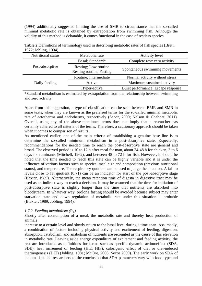
11

(1994) additionally suggested limiting the use of SMR to circumstance that the so-called minimal metabolic rate is obtained by extrapolation from swimming fish. Although the validity of this method is debatable, it comes functional in the case of restless species. Table 2 Definitions of terminology used in describing metabolic rates of fish species (Brett, 1972; Jobling, 1994)

Nutritional status Metabolic rate Activity level

Post-absorptive Basal; Standard* Complete rest: zero activity

Resting; Low routine Resting routine; Fasting Spontaneous swimming movements

Daily feeding Routine; Intermediate Normal activity without stress

Active Maximum sustained activity Hyper-active Burst performance; Escape response

*Standard metabolism is estimated by extrapolation from the relationship between swimming and zero activity. Apart from this suggestion, a type of classification can be seen between BMR and SMR in some texts, when they are known as the preferred terms for the so-called minimal metabolic rate of ectotherms and endotherms, respectively (Secor, 2009; Nelson & Chaboat, 2011). Overall, using any of the above-mentioned terms does not imply that a researcher has certainly adhered to all criteria of the terms. Therefore, a cautionary approach should be taken when it comes to comparison of results. As mentioned earlier, one of the main criteria of establishing a genuine base line is to determine the so-called minimum metabolism in a post-absorptive state. Expectedly, recommendations for the needed time to reach the post-absorptive state are general and broad. The observed period is 10 to 12 h after meal for man, about 24-48 h for chicken, 3 to 6 days for ruminants (Mitchell, 1962), and between 48 to 72 h for fish. However, it should be noted that the time needed to reach this state can be highly variable and it is under the influence of various factors such as species, meal size and composition (previous nutritional status), and temperature. The respiratory quotient can be used to judge the situation. A fall to levels close to fat quotient (0.71) can be an indicator for start of the post-absorptive stage (Baxter, 1989). Alternatively, the mean retention time of digesta in digestive tract may be used as an indirect way to reach a decision. It may be assumed that the time for initiation of post-absorptive state is slightly longer than the time that nutrients are absorbed into bloodstream. In whatever way, prolong fasting should be avoided because subject may enter starvation state and down regulation of metabolic rate under this situation is probable (Blaxter, 1989; Jobling, 1994). 1.7.2. Feeding metabolism (RF) Shortly after consumption of a meal, the metabolic rate and thereby heat production of animals increase to a certain level and slowly return to the basal level during a time span. Assumedly, a combination of factors including physical activity and excitement of feeding, digestion, absorption, catabolism, and anabolism of nutrients are recounted as the cause of this elevation in metabolic rate. Leaving aside energy expenditure of excitement and feeding activity, the rest are introduced as definitions for terms such as specific dynamic action/effect (SDA, SDE), heat increment of feeding (HiE, HIF), calorigenic effect of diet or diet-induced thermogenesis (DIT) (Jobling, 1981; McCue, 2006; Secor 2009). The early work on SDA of mammalians led researchers to the conclusion that SDA parameters vary with food type and

12

ration size, and if substrates are fed separately, the heat loss by animals corresponds to 30% of the caloric content of protein 13% of lipid and 5% of carbohydrate. In an attempt to devise a mathematical model for total metabolism of fish, Kerr (1971) wrote TC= mR, where TC is the energy cost specific to utilization of food (or in other words, SDA) R is ingested ration and m a constant within the range corresponding to a 60 to 70% of feed conversion efficiency. Weatherly (1976) used the same formula and wrote that the constant m varies with diet composition and reach a maximum of 0.3 for a pure protein diet. In another attempt, Jobling (1985), based on some new evidence (summarized in Jobling 1981, 1983), proposed a new relation between SDA and growth: RF=rP , where P is growth (production) and r the energy cost per unit growth. The difference between two views is fundamental. The first formula introduces SDA and growth as competitors. It means if a diet induces higher SDA and therefore higher loss of energy as heat, it promotes less growth. Conversely, the second formula has an interactive view to SDA and growth; the higher the growth is, higher the SDA would be. In other words, a diet that improves growth should cause higher SDA as well. Lucas (1992) brought this view into question and argued that a large proportion of protein in the diet of fish results in two effects; elevated growth and escalated SDA. Nevertheless, a pure protein diet can increase the SDA further but not growth. The conclusion that can be drawn from these discussions is that the relation between SDA and growth might be linear only under certain conditions and both of the above-mentioned relations may be true under certain circumstances. For measuring SDA, animal must be given a specified quantity of a test diet and afterward the postprandial metabolic response is recorded continuously or intermittently as long as the metabolic rate returns to a pre-defined basal rate. Using indirect calorimetry method, SDA is obtained by summation of the above-baseline oxygen consumption (OC) or produced CO2. Afterward, the total OC is multiplied by a suitable energy-converting coefficient. On which basis and for which purpose SDA is reported is very dependent on the objectives of studies. Different factors including temperature, body weight, feed quality, and quantity can influence SDA. On the other hand, the duration, magnitude, and peak of SDA (SDAMax) in response to influential factors are of interest (Jobling, 1981; McCue, 2006; Secor, 2009). A hypothetical graph of SDA when metabolic rate is plotted against post feeding time presents in Figure 3. SDA may be reported as factorial increase in metabolic rate, which may be called SDA scope or factorial scope (SDAMax/ Rs). This scope is useful when it is compared with maximal metabolic scope, and it signifies how much extra power is available for animals’ activity during feed assimilation. A more bioenergetics relevant approach for reporting SDA is SDA coefficient (CSDA). In this technique, the allotted energy to SDA (ESDA) is divided to meal energy (Emeal) and reported in percentage (CSDA= [ESDA/ Emeal] ×100). Therefore, CSDA shows the percentage of feed energy that is used for the assimilation of the given feed. CSDA is broadly used to compare study results regardless of body mass, species, meal type, and size. However, there are two main objections to such comparison. First, the relation between SDA and ingested energy is an allometric relation rather than isometric. Therefore, standardization to unit of meal energy will lead to estimation error. Second, by use of CSDA, it is assumed that SDA is independent of body mass, which is a false assumption. On this basis, CSDA can only be used trustworthily for intraspecific comparison when animals with similar body mass are fed identical diets (i.e. isoenergetic) (Beaupre, 2005; Secor and Boehm 2006; McCue2006; Secor 2009).

13

Figure 3 A hypothetical SDA graph (adapted from Jobling, 1981; Score, 2009).

1.8. A short review of different respirometers Respirometers with different designs and various methods have been used to measure SDA and gas exchange of aquatic animals. Leaving aside the tunnel respirometers that are used to measure active/swimming metabolic rate, three other types of laboratorial respirometers exist. Close/ static respirometers are mostly useful for short time measuring of OC. The main problem in using these types of respirometers is the accumulation of metabolites such as CO2 and ammonia, which may affect OC. Therefore, using them is not recommended for long time studies of OC (Forstner 1983; Steffensen, 1989). Intermittent flow-through or intermittent closed respirometers are another type of respirometers that are in use (Forstner, 1983; Fischer, 2000; Zimmermann1& Kunzmann, 2001; Schleuter et al., 2007; Eliason et al., 2008; Millidine et al., 2009; Bilberg et al, 2010; Cai et al., 2010; Vanella et al., 2010; Voutilainen et al, 2011). The design of these respirometers makes it possible to flush system intermittently and discharge the built up metabolites. These respirometers are most often equipped with automatic valves to create a combination of flushing and static states. The target parameters are measured during static state. The transit time between static and flushing state is indeed dependent on respirometer/fish size. Researcher needs to ensure that oxygen and ammonia levels remains at appropriate levels during the whole period of an experiment. The third type of respirometers is Flow-through open respirometers or continuous flow respirometers (Preez et al., 1986; Chakraborty et al, 1992; Forsberg 1997; Zakus et al, 2003; Fu et al., 2005; Fu et al, 2006; Finstad et al, 2007; Luo& Xie 2008; Stejskal et al, 2009; Pang et al., 2010; Leeuwen, 2012; Wang, 2012). In this types of respirometry, water flows constantly during the experiment. The inflow adjusts to cause certain reduction in the level of oxygen in respirometers but oxygen level will remain well above critical level. The oxygen levels of inflow and outflow water are measured continuously or periodically and the differences are reported as OC. This respirometry method has the advantage of continues measurement of OC without accumulation of waste metabolites. However, interpreting the data coming from these experiments may demand more corrections. Flow rate is a part of the calculation formula. It should remain constant during measurement and it should be continuously measured to ensure a constant rate. If open respirometers are used (i.e. a simple flow-through tank with open surface) the possibility of oxygen exchange with the environment should be considered. Another problem that may arise when using flow through system is difficulty in measuring ammonia excretion when an individual fish is placed in the respirometer.

Peak

Baseline

Time to peak Feeding

Duration Baseline (i.e.FMR)

Metab

olic r

ate

Post feeding time

SDA

14

The aim of this thesis The aim of this study was to feed fish different carbohydrate levels and evaluate whether it is possible to determine the appropriate level of carbohydrate in diet of fish by measuring energy expenditure and metabolic rate of fish through OC and ammonia excretion (AE). We hypothesized that if digestion and assimilation of high level of carbohydrate in diet exerts pressure on fish, it should lead to higher metabolic rate and heat production. We also hypothesized that ammonium excretion will be affected by different inclusion level of carbohydrate in the diet and a protein sparing effect will be observed. Conversely, if there is no difference in OC, fish can digest and utilize all levels of the given carbohydrate without problem. Additionally, we conducted this project along with a digestibility experiment for further comparison.

2. Materials and methods

2.1. Experimental fish and acclimation Eurasian perch fingerlings of second generation were bought from a commercial fish hatchery (Östgös AB, Söderköping, Sweden). The fish were reared for 18 months in the fish laboratory of the Department of Animal Nutrition and Management, SLU, Uppsala. During the rearing period, fish were fed by commercial diets (BioMar EFICO Alpha 714) and kept inside a plastic tank in a flow-through system. Four Eurasian perch, two 145g and two 150 g, were selected for this experiment. The chosen fish were transferred to four separate respirometers (see below) and held inside the chamber for 50 days before the start of measurement. Transferred fish were fed with a small amount of commercial feed by hand for one week. Afterward, fish were trained to consume commercial feed inside gelatin capsules (the capsule properties can be seen in Table 4). The capsules were placed on nets and inserted to the chambers. Additionally, a daily routine of siphoning out the feces and water change was practiced.

2.2. Facilities and measuring devices: 2.2.1. Respirometer Four square-shape respirometers were designed for this experiment. Chambers’ walls and bottoms were made of glass. Lids were made of hard transparent plastic. The chambers were part of a recirculation system which consisted of two reservoir buckets (upper and lower) with the capacity of 35L each and four 20 L chambers (35 cm (L):24 cm (H) :24cm (W)). Water flowed through pipes into chambers with aid of static pressure. Discharged water was filtered by passing through sponges and LECA balls (Light Expanded Clay Aggregate) and then collected in the bottom reservoir bucket for pumping to upper reservoir. Each chamber possessed an opening (5 cm in diameter) on the lid for inserting electrodes and feeding purposes. The inlets and outlets of all chambers were separate and independently adjustable. Each chamber was equipped with a pump to simulate the stirring effect and prevent stratification of gas content during measurement (Figure 4). A curtain was also installed in front of the chambers to secure fish from surrounding area and prevent visual stress on them.

15

Figure 4 A schematic picture of respirometers. 1.Upper reservoir bucket 2. Respirometers 3. Opening for feeding and inserting electrodes, 4. inlet, 5. Outlet, 6. Filter, 7. Sponges, 8. LECA balls, 9. Pumps for recirculating chambers water during measurement, 10. The main recirculation pump 11. Lower reservoir bucket. =Valves, Arrows show water flow direction. 2.2.2. Measurement devices Two HQ40d Portable Multi-Parameter Meter (Hach Lange AB, Sköndal, Sweden) were used for measuring oxygen level. Each meter was equipped with two IntelliCAL™ LDO101 Standard Luminescent Dissolved Oxygen Probes (detection range: 0.1 - 20.0 mg L-1, accuracy: ±0.1 mg L-1 for 0 to 8 mg L-1 and ±0.2 mg L-1 for greater than 8 mg L-1). One IntelliCAL™ PHC101 Standard Gel Filled pH Electrode connected to HQ40d was used for pH measurement. For ammonium measurement, ELIT 8 Channel Ion/pH Analyzers (NICO2000 Ltd, London, UK) and its ammonium Ion-Selective electrodes (Concentration range: 0.03 to 1.8 ppm) were used.

2.3. Experimental feed Four experimental diets with 0, 10, 20, and 30% starch contents were formulated for this study. Feed ingredients and proximate analysis are presented in Table 3. Samples of feed ingredients, and diets were analyzed with standard methods (AOAC, 1997). Dry matter was determined by drying in an oven at 1050 C for 24 h. Nitrogen content was determined by the

16

Kjeldahl method and crude protein was calculated as N x 6.25. Crude fat content was analyzed using the Soxhlet method after acid hydrolysis of the sample. Ash content was determined by incineration in a muffle furnace at 5500 C for 12 h. Gross energy (MJ kg-1) was determined with a bomb calorimeter (Calorimeter Parr 6300, Parr Instrument Company, Moline, IL, USA). Table3 Composition and proximate analyses of experimental diets

a.Vitamins (mg kg-1): , Vitamin E, 40000; K3, 2000; B1, 3000; B2, 5000; B6, 3000; B12, 4.0; B5, 6000; B9, 1000; Biotin, 50; C, 25000; Vitamin A, 500 IE/g; D3, 300 IE/g. Minerals: (mg kg-1): cobalt sulphate, 200; copper sulphate, 1000; calcium iodate, 600; manganese sulphate, 3000; zinc sulphate, 24000; calcium 220000. All diet ingredients except gelatin were initially mixed together. Gelatin was subsequently added to the pre-mixed feed ingredients and the dough was grinded with a 2mm sieve to form strings. The strings were placed inside refrigerator for 1h at 2̊ C and then dried for approximately 3h at 50̊ C. After 3 h, strings were chopped to small size pellets and transferred to the drying cabinet again for further drying (3 h or until being judged as dried). The pelleted feeds were stored at -25̊ C until being used. At feeding time, the pellets were converted to powder with a coffee grinder, and capsules were filled up with powder (Table 4). Table 4 Physical specifications and proximate analyses (g kg -1 DM) of empty gelatin capsule size 0.

a As demonstrates with provider’s website (http://www.capsuleworld.com/).

Dietary starch content (%) Ingredients (g/kg diet) 0 10 20 30 Wheat starch 0.00 100 200 300 Fish meal 500 560 500 470 Gelatin 71.4 80 71.4 67 Lipid 158.6 130 85 20 Lecithin 10 10 10 10 Titanium dioxide 5 5 5 5 Cellulose 250 121.43 123.6 123 Mineral vitamin Premixa 5 5 5 5 Proximate analysis (g/kg DM) Dry Matter % 95.50 94.30 95.10 94.90 Ash 76 82 76 74 Crude protein 445 495 453 428 Crude fat 201 197 152 84 Starch 6 92 186 284 Gross energy (MJ/kg diet) 22.46 22.06 20.08 19.41

Outer diameter (mm) 7.65a Gross energy (MJ/kg) 18.58 Height or Locked Length (mm) 21.7a DM% 87.30 Actual Volume (ml) 0.68a Ash 19 Typical Fill Weights(mg) 0.70 Powder Density

475a Crude protein 987b

Empty capsule weight (g) 0.10 Crude protein in one capsule 0.09b Capsule weight +experimental feed (g) ~0.50

17

b The values were calculated based on nitrogen conversion factor of 5.55 for gelatin.

2.4. Experimental procedures The experiment was run for five weeks. Four weeks were assigned to the test diets. One week was used for measuring FMR. The routines for each week consisted of three consecutive feeding days, one starvation day, and two sequential after feeding-measuring days. FMR values were achieved in week five after starving fish for 24 hours. Each measuring session lasted for 7 h 30 min. At the end of the experiment, a 7-h measurement was performed in the absence of fish to determine errors that might be caused by probable devices’ drift or microorganisms. Every measuring day started by feeding fish with capsules. Each fish received two capsules (0.50 g /capsule) on the feeding days and three capsules (1.50 g; ca 1% of body weight) on measuring days. Fifteen minutes were given to fish to consume the capsules. If fish did not consume the capsules during the given time, the capsules were taken out. A camera was installed to supervise feeding activity and fish behavior. Fifteen minutes after feeding feces were siphoned. At the experiment day, water from a container (150 L) outside of the recirculation system was used to change chambers’ water. The container water pH was reduced to approximately 6.50 with HCl before adding to chambers (ca 130-140ml 1M HCl to 150 L water). The reason for reducing pH was to have ammonia in ionized from, NH4+. The reaction NH3+ + H+↔NH4+ + OH- is favored toward NH4+ at pH levels less than 7 and negligible amounts of NH3+ remains in water. NH4+ is less toxic to fish compared to NH3+. In addition, our electrodes were only able to measure ammonium. Changing water with the slightly acidified water provided chambers with a pH range of 6.5 to 6.8. The water was changed by pumping up acidified water to the upper bucket from the 150 L container. Outlets were closed and respirometers were filled up with water completely. The openings of the chambers were blocked with sponges to reduce oxygen transport between the air and the water surface. The electrodes were crossed through sponges into the chambers and left in their place for the whole measurement period. Four ammonium and four oxygen electrodes (one for each chamber) were used. Just before the start of measurement, the ammonium electrodes were first immersed in a 1000 ppm standard solution (NH4Cl) for 10 minutes. Then, they were calibrated for 0.010, 0.10, 1.0, and 10.0 ppm concentrations by immersing them in the related standard solutions for 5 minutes and recording the millivolts (8-channel ion analyzer software). The signal averaging number (the number of readings that is taken and an average is produced as the final millivolt/read) for ammonium analyzer was adjusted to 300 seconds and for dissolved oxygen to 90 seconds. The first values were recorded 30min after feeding. Oxygen concentrations were recorded every 15 min and nitrogen concentrations were recorded every 30 min. When the oxygen levels were reduced to 6 mg L-

1, chambers were oxygenated by a mixture of pure oxygen and air for about 10 minutes. The chambers’ water pH was measured twice; once after changing water and another time at the end of the run. A weekly calibration for the pH electrode was performed as well. The water temperature during whole acclimatization and experimental periods were 18±1̊ C.

2.5. Calculation and statistical procedure The consumption of three capsules in measuring days was the criterion for including the obtained data from each fish in calculation. Therefore, the data from one fish was completely omitted due to refusal of feed. Microsoft Excel was used for primary calculations. The obtained values from blank (without fish) respirometers were used to correct the values of every run. OC (mg min-1 kg-1 BW) was calculated according to the formula suggested by

18

Steffensen (1989): MO2=Vr × ∆CWO2

∆t × BW, where MO2 is total oxygen consumption per unit of the

body mass (mg O2 min-1 kg-1 BW), Vr is the water volume in the respirometer minus fish volume (L) ∆CWO2 is the change in water oxygen concentration (mg O2 L-1) BW is body weight (kg), and ∆t is the time interval of measuring (min). A similar formula was used for calculation of ammonia excretion (AE(min/kg/ BW) = Vr × ∆AE

∆t × BW ). As the exact BWs of fish

before each run were not available and using any other weight should have been based on assumption, calculations were performed by the end weights of fish. The end weights for the two 145 g fish were 185 and 200 g and for the two 150 g fish were 218 and 183 g. The calculated values Data were analyzed with the Statistical Analysis System, version 9.2 (SAS Institute, Cary, NC, USA) with Proc Mixed. The model included the fixed factors of diet (0%, 10%, 20% and 30% starch) and day (day1 and day2) and the interaction between diet and day. The results are presented as Least Square means ± S.E.M. and the statistical significance level is set to P<0.05.

3. Results

3.1. Oxygen consumption No interaction between days and diets was observed. Hence, interaction was excluded from the statistical model. Table 5 presents the least square mean values of OC for the tested diets. Whereas mean values of OC decreased numerically from diet 0% to 30% Starch, the diets used in this experiment had no statistically significant impact on OC (P= 0.174). In contrast, there was a significant effect of the days on OC (P=0.001). Fish consumed more oxygen on the second days of measurements. It is reasonable to assume that the peak that occurs shortly after feeding (or in our case, shortly after the start of measurement) is a reflection of feeding, ingestion activity, and probable stress, while it was not related to diet composition. It should be noted that the observations at 45 min after feeding is equivalent with 15 min after the start of measurement. Consequently, the term feed (composition)-related peak was used in this paper to avoid confusion. The first recorded observation showed elevated OC after feeding. Afterwards, OC decreased until 3 to 4 hours after feeding (Figure 5). A second increase in OC was observed around 4 h after feeding. The magnitudes of peaks (MOP) were higher on the second days of measurements (Table 6). There was an apparent forward shift of peak times as starch level increased, which was more obvious during the first days of measurements. There was higher fluctuation in OC during the days that fish received diet 0% Starch. Table 5 Least Square Means (LSM) of two days Oxygen Consumption (OC, mg min-1 kg-

1BW) in relation to different diets. Diets P value 0% Starch 10% Starch 20% Starch 30% Starch OC 1.616a 1.490a 1.346a 1.149a 0.174 SEM1 0.138 0.137 0.137 0.137 Days 1 2 OC 1.272a 1.528b 0.001 SEM1 0.074 0.071 aValues in row with the same superscripts are not significantly different (p>0.05).

19

1SEM= Standard Error of the Mean. Table 6 Post feeding time (PFT; h:min) and magnitude of peak (MOP; mg. min-1 kg BW-1) of oxygen consumption (OC) and ammonia excretion (AE) for two days and each diet.

Diet 0%

Diet 10%

Diet 20%

Diet 30%

Day 1 Day 2 Day 1 Day 2 Day 1 Day 2 Day 1 Day 2 PFTOC 4.45 6:15 4:30 4:45 5:30 5:30 6:45 6:45 MOPOC 2.59 3.13 1.60 1.98 1.43 2.25 1.46 1.85 PFTAE 5:00 4:00 6:30 6:00 6:00 4:30 6:30 4:30 MOPAE 0.32 0.58 0.30 0.21 0.25 0.29 0.25 0.27

20

Figure 5 Oxygen consumption profiles (Mean ±SD mg. min-1. kg BW-1 OC) of Eurasian perch in two separate days for each diet in every 15 min. Post feeding time starts from 45 min after feeding.

3.2. Ammonia excretion During the two initial hours of all runs, data from the ammonium device showed no increase in water ammonium concentration (AE ≈ zero). Therefore, the results of AE are presented from 2 h after feeding and onwards. There was no or very little AE during starvation. Table 7 presents the LSM values of AE. Statistical analyses showed that only differences between mean values of diets 0% and 10% Starch were significant (P= 0.04). Consumption of diet 10% Starch led to the least AE compared to the other diets. The mean value of AE for diet 20% and 30% Starch were numerically slightly lower than AE for diet 0% Starch, and those were slightly higher than AE for diet 10% Starch, but no statistically significant difference between these diets were observed. Additionally, there was no significant difference between experimental days. Table 7 Least Square Means (LSM) of 2 days ammonia excretion (mg min-1 kg-1BW) in relation to different diets. Diets P value 0% Starch 10% Starch 20% Starch 30% Starch AE 0.21a 0.16b 0.18ab 0.20ab 0.04 SEM1 0.01 0.01 0.01 0.01 Days 1 2 AE 017a 0.20a 0.13

21

SEM1 0.01 0.01 aValues in row with the same superscripts are not significantly different (p>0.05). 1SE= Standard Error of the Mean. Around 2 h after feeding the excretion of ammonia became evident. The peaks of AE occurred 4 to 6 h after feeding (Table 6). On the second days, the peaks of measurements occurred sooner than the peaks during the first days of measurements. Diet 0% Starch had the highest peak magnitude and AE fluctuation during the second day of measurement on this diet was higher than other runs as well (Figure 6).

22

Figure 6 Ammonia excretion (AE) profiles (Mean ±SD mg. min-1. kg BW-1 AE) of Eurasian perch in two separate days for each diet in every 30 min. Post feeding time starts from 2 h after feeding.

4. Discussion Previously, it has been shown that magnitude of SDA is highly dependent upon diet composition, particularly protein content (Medland & Beamish, 1985; Beamish & Trippel, 1990 Brown & Cameron 1991, Ross et al., 1992; Fu, 2005). Research on warm-blooded (homoeothermic) animals indicates that the heat production that originated from feed consumption is identical to 30% of the caloric content of protein, 13% of lipid, and 5% of the caloric content of carbohydrates. However, these values may not directly apply to animals like fish that mostly excretes ammonia in form of ammonia and physiologically shows distinct differentiation from mammals (Smith et al., 1978). The result of our experiment showed that no significant change in OC occurs when starch level increases up to 30 % at the expense of lipid content. Even so, two factors should be taken into account here. First, as the time lengths of the conducted runs were not long enough to allow values to return to basal metabolic rate, therefore, one may be skeptical about the ineffectiveness of carbohydrate level on all parameters of SDA. The results presented in this study remain open to interpretation at least when it shows an apparent shift in time of peak and a tendency for a longer SDA duration with increased starch levels. Second, a non-significant effect on SDA can also indicate that starch was not well digested. Inadequate digestion means no utilization and hence, no effect on SDA. Some other studies have also shown the phenomenon of no or very small effect of raw starch on SDA. Fu et al. (2007) tested the effect of purified protein, carbohydrate and lipid on the SDA of catfish. Their result showed that the SDA coefficient for protein was higher than lipid (9.41% vs. 7.43%), and both were higher than the SDA

23

coefficient for raw starch, which gave a coefficient of close to zero (0.84%). In contrast, when Fu et al. (2005) gave catfish a gelatinized starch at the expense of protein (one diet contained 30% protein, 30% starch, and another diet 50% protein, 0% starch), they found no difference between SDA coefficients of the two test diets. The assumption that starch may be utilized with near 100% efficiency does not seem realistic. Conversely, presuming that carnivore fish utilize starch and protein with similar energy efficiency may be reasonable. Smith et al. (1978) tested the effect of purified nutrients on heat production of rainbow trout and Atlantic salmon, using direct calorimetry. Based on the obtained results, they concluded that the HI of carbohydrate (dextrin) and protein (casein) were not significantly different and both were higher than HI of fat. The major, but maybe not the only probable reason behind this phenomenon is the cost-effectiveness of ammonia excretion in fish. In comparison to fish that excrete about 85% of waste ammonia in form of ammonia through the gills, terrestrial homeotherms face the extra costs of synthesizing, concentrating, and excreting of urea/uric acid by the kidneys. Overall, the results obtained in the present study suggest that the tested raw starch was not digested properly and therefore caused no impact on SDA. Based on the results of AE, it seems the portion of digested starch was not enough to prevent protein from being oxidized. However, to have a clearer picture of protein-carbohydrate interaction during utilization, data on starch digestibility are needed. It is obvious from the results of this study that determining an accurate peak, particularly for OC, is not an easy task. Although the occurrence of an elevated level of OC shortly after feeding is common, the appearance of this phenomenon even during starvation can infer the existence of an additional factor besides feeding activity. Our practice to measure oxygen consumption directly inside the chamber could be an extra stressor for fish. Consequently, the combined effect of stress and feeding activity in some cases led to a relatively high oxygen consumption rate during the first hours after start of measurement. A study by Acerete et al. (2004) on Eurasian perch showed an immediate increase in cortisol levels 0.5 h after handling, a peak of secretion 2 h after handling (121 ng ml-1) and a return to the basal level (45 ng ml-1) after 4 h, as treatments compared with a control group, acclimated for 21 days. However, it should be noted that a basal level of 45 ng ml-1 for cortisol could be far away from a normal basal level. For example, trout shows a mean basal value of 1.7 ng ml-1, carp 7.4 ng ml-1, and yellow perch shows values between 4 to 8 ng ml-1. A high level of blood cortisol indicates that perch is prone to develop a chronic state to stressors under culture/ laboratory condition. Secretion of cortisol in response to stress may also lead to different secondary responses such as release of glucose and/or lactate into the blood and change in hematocrit values to overcome the increased metabolic demands. In the study of Acerete et al. (2004), increased cortisol levels were not followed by a significant increase in the blood lactate concentration. Therefore, the possibility of taking advantage from anaerobic metabolism was absent. In contrast, handling stress caused an increase in the number of red blood cells. An increase in erythrocyte numbers for enhancing the efficiency of oxygen transport is apparently the strategy that perch use in case of encountering short acute stress. Because of this strategy, alteration in oxygen consumption of perch during 2 to 3 h after stress can be expected. One of the main issues in reporting feed-related oxygen consumption is the difficulty of separating spontaneous activities from true SDA. Any type of activity by fish during measurement can change the magnitude of OC and may cause misinterpretation of peak values and feed related OC. According to Jobling (1981), this phenomenon might be well fitted to the position of responsibility for variation in reported SDA for a specific fish. In the present study, OC showed high fluctuation during the days that diet 0% Starch was given. At least one fish was more active than other fish, and the consequence of these activities appeared in higher oxygen consumption by this fish and a large SD. As shown in Figure 5,

24

the peak of OC on the second day of measurement on the diet 0% Starch appeared 6 h 15 min after feeding. This peak does not seem to be correct because the adjacent OC are not matched with this peak. Generally, a short measuring interval can help to notice sudden fluctuations while these events may simply remain invisible if measuring interval is long or reported in long interval. The fluctuations in OC suggest that fish were perhaps more active during some runs of our study. However, a sound and reliable interpretation may demand using technologies like video cameras and recording the runs. Additionally, if measuring interval is short, it should be possible to correct theses values according to adjacent OC or totally omit them from results. In the present study, the feed-related OC peak ranged from four to six hours post feeding. These results are comparable with the results of Stejskal et al. (2009) who measured perch OC every 2 h in a flow-through system and reported the occurrence of OC peak 6 h after onset of feeding. It is noteworthy that the size of ∆t seems to affect the reported/observed peak times. For instance, reporting our results on an hourly basis can lead to a 30 min to 1h forward shift of peak time. Zakus et al. (2003) reported that perch OC returned to the basal level 6 h after termination of feeding. In the present study, OC remained well above the basal level even 7 h after feeding. The aforementioned author employed continuous feeding in their study. Noble (1973) investigated the effect of continues feeding and single meal on gastric evacuation rate of young yellow perch. The results showed that the evacuation rate under continuous feeding is almost two times faster than that under single meal feeding (6 h vs. 12 h). Therefore, it might be possible that continuous feeding in study of Zakus et al. (2003) resulted in return of metabolic rate to the basal level in a shorter period. Inclusion of starch in the present study did not lead to significant change in AE, except for diet 10% Starch. Again, we must emphasize that inadequate length of the runs makes interpretation of results doubtful. However, it is interesting that only diet 10% Starch exhibited a protein sparing effect. In addition to starch, the lipid contents showed the main difference between diets. While lipid contents of diets 0% and 10% Starch were almost the same (200 g kg-1 DM), the lipid level decreased by 50 and 116 g kg-1 DM for diet 20% and 30% Starch, respectively. Assuming that the raw starch remains largely undigested, the consequence of increased level of starch would be an increase in digestible protein: energy ratio (DP: DE). In this case, there would be an alteration in the ratio of non-protein and protein source energy. As lipid content of diet 10% Starch was relatively high and similar to diet 0 % Starch, extra energy coming from starch digestion could have been enough to prevent protein oxidation (or promote protein synthesis), and consequently diminish AE. On the contrary, for diets 20% and 30%, Starch, there were not enough sources of non-protein energy when the lipid contents of the diets decreased and were not replaced by another energy source. Due to lack of non-protein energy source, the body will start to oxidize protein to cover energy needs. This hypothesis may be fortified by the numerical data achieved from AE. The data showed an increase in AE from 10% Starch to 30 % Starch and the AE of diet 30% Starch became almost similar to 0% starch (0.20 vs. 0.21mg min-1 kg-1). This reverse action is probably the reason for non-significant difference between diets 10%, 20%, and 30% Starch. Another issue that can be addressed here is the effect of starch level on its own digestibility and digestibility of other nutrients. Hemre et al. (1995) fed Atlantic salmon with different starch levels, ranging from 0% to 31%. Their results showed that digestibility of starch significantly dropped when the inclusion level reached 22% (Table 8). Moreover, increased starch level caused a decrease in lipid digestion, but the effect of inclusion level was non-significant for protein apparent digestibility. Based on this information, the undigested starch may affect lipid digestion in a similar way to dietary fiber, which can increase the viscosity of digesta and impair lipid digestion.

25

Table 8 Apparent digestibility (percentage) of dietary components in Atlantic salmon fed diets with increasing starch content. Hemre et al. (1995)

a.b Significant difference at P < 0.05 The peaks of AE in current study ranged from 4 h to 6 h 30 min after feeding. These results were not in agreement with the reported peak by Stejskal et al. (2009), which was 8 h after the onset of feeding, but were comparable to a study by Zakes et al., (2003). The latter authors reported an increase in both OC and AE 2–3 h after the start of feeding and a peak for both OC and AE 6–7 h post feeding. However, the variation between reported peaks in different studies should be considered a normal event because factors such as meal size and quality, temperature and feeding frequency can affect the peak magnitude and time (Ross et al, 1992; Lu & Xie 2009). Previously, several studies reported similarities between AE and OC patterns and concurrency of peaks in different species (Clarke & Thomas, 1997; Alsop & Wood 1997; Owen et al., 1998). Such similarity is observable for the second measurement days of diet 0% Starch, when both AE and OC patterns had high fluctuations. Additionally, the times of peaks for OC and AE of diets 0%, 20% and 30% Starch on the first days of measurements were close. On the second days of measurement, nonetheless, AE showed different correlation with OC and the peak of AE occurred hours sooner than peak of OC. Lu & Xie (2009) experienced this phenomenon in their experiment on catfish. While they tried to introduce this phenomenon as a probable characteristic of catfish, the present results suggest that this might be due to an external factor. The results of this study showed a correlation between magnitude of OC (metabolic rate) and the peak time of ammonia excretion. On the second day of measurement for each diet, when the magnitude of OC peak was higher, the peak of AE occurred earlier. As the peak occurred shortly after feeding (4 h 30 min), it is likely that part of this ammonia originates from muscle breakdown rather than feed. Moreover, regarding the second day of diet 20% Starch, the magnitude of the peak at 6 h 30 min after feeding is the same as that of at 4 h 30 min post feeding, which can be an indicator of a feed-related peak.

5. Conclusion The results of this experiment showed that inclusion of raw starch in the diet of Eurasian perch dose not lead to change in oxygen consumption (OC). Therefore, it is possible that

Dietary starch levels (%) 0 5 9 22 31 P-value Dry matter 91 91 90 87a 83b 0.003 Protein 95 95 94 94 93 n.s. Lipid 94 95 94 92 89 0.040 Starch - 91 93 75b 76 0.003

26

inclusion of raw starch with up to 30% in the diet of this fish species does not exert any significant effect on the metabolic rate. Additionally, it became evident that levels up to 10% Starch can have a protein sparing effect. It can be recommended from the result of this study to include up to 10% raw starch in the diet of Eurasian perch. Moreover, future calorimetric studies should preferably be performed for longer time to allow the metabolic rate to return to basal level. Furthermore, the results of digestibility traits should be used along with results from calorimetric studies to allow calculations of substrates available for metabolism.

References

Acerete L., Balasch J.C., Espinos E., Josa A., and Tort L., 2004. Physiological responses in Eurasian perch (Perca fluviatilis, L.) subjected to stress by transport and handling. Aquaculture 237, 167–178.

Ai Q., Xie X., 2006. Effects of dietary soybean protein levels on metabolic response of the southern catfish, Silurus meridionalis. Comp. Biochem. Physiol. A, 144, Pp.41–47.

AOAC., 1997. Methods of Analysis of Association of Official Agricultural Chemists. , Association of Official Analytical Chemists, Washington, DC.

Beamish F. W. H. and Trippel E. A., 1990. Heat Increment: A Static or Dynamic Dimension in Bioenergetic Models? Transactions of the American Fisheries Society, 119,4, 649-66.

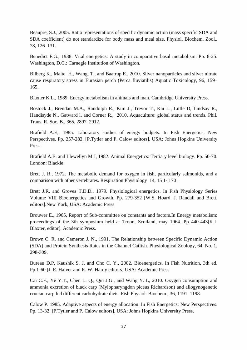
27

Beaupre, S.J., 2005. Ratio representations of specific dynamic action (mass specific SDA and SDA coefficient) do not standardize for body mass and meal size. Physiol. Biochem. Zool., 78, 126–131.

Benedict F.G., 1938. Vital energetics: A study in comparative basal metabolism. Pp. 8-25. Washington, D.C.: Carnegie Institution of Washington.

Bilberg K., Malte H., Wang, T., and Baatrup E., 2010. Silver nanoparticles and silver nitrate cause respiratory stress in Eurasian perch (Perca fluviatilis) Aquatic Toxicology, 96, 159–165.

Blaxter K.L., 1989. Energy metabolism in animals and man. Cambridge University Press.

Bostock J., Brendan M.A., Randolph R., Kim J., Trevor T., Kai L., Little D, Lindsay R., Handisyde N., Gatward l. and Corner R., 2010. Aquaculture: global status and trends. Phil. Trans. R. Soc. B., 365, 2897–2912.

Brafield A.E,. 1985. Laboratory studies of energy budgets. In Fish Energetics: New Perspectives. Pp. 257-282. [P.Tytler and P. Calow editors]. USA: Johns Hopkins University Press.

Brafield A.E. and Llewellyn M.J, 1982. Animal Energetics: Tertiary level biology. Pp. 50-70. London: Blackie

Brett J. R., 1972. The metabolic demand for oxygen in fish, particularly salmonids, and a comparison with other vertebrates. Respiration Physiology 14, 15 1- 170 .

Brett J.R. and Groves T.D.D., 1979. Physiological energetics. In Fish Physiology Series Volume VIII Bioenergetics and Growth. Pp. 279-352 [W.S. Hoard .J. Randall and Brett, editors].New York, USA: Academic Press

Brouwer E., 1965, Report of Sub-committee on constants and factors.In Energy metabolism: proceedings of the 3th symposium held at Troon, Scotland, may 1964. Pp 440-443[K.L Blaxter, editor]. Academic Press.

Brown C. R. and Cameron J. N., 1991. The Relationship between Specific Dynamic Action (SDA) and Protein Synthesis Rates in the Channel Catfish. Physiological Zoology, 64, No. 1, 298-309.

Bureau D.P, Kaushik S. J. and Cho C. Y., 2002. Bioenergetics. In Fish Nutrition, 3th ed. Pp.1-60 [J. E. Halver and R. W. Hardy editors] USA: Academic Press

Cai C.F., Ye Y.T., Chen L. Q., Qin J.G., and Wang Y. L, 2010. Oxygen consumption and ammonia excretion of black carp (Mylopharyngdon piceus Richardson) and allogynogenetic crucian carp fed different carbohydrate diets. Fish Physiol. Biochem., 36, 1191–1198.

Calow P. 1985. Adaptive aspects of energy allocation. In Fish Energetics: New Perspectives. Pp. 13-32. [P.Tytler and P. Calow editors]. USA: Johns Hopkins University Press.

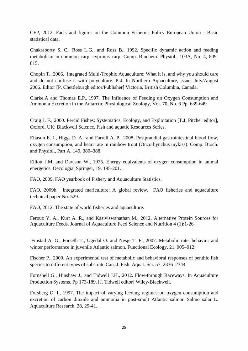
28

CFP, 2012. Facts and figures on the Common Fisheries Policy European Union - Basic statistical data.

Chakraborty S. C., Ross L.G., and Ross B., 1992. Specific dynamic action and feeding metabolism in common carp, cyprinus carp. Comp. Biochem. Physiol., 103A, No. 4, 809-815.

Chopin T., 2006. Integrated Multi-Trophic Aquaculture: What it is, and why you should care and do not confuse it with polyculture. P.4. In Northern Aquaculture, issue: July/August 2006. Editor [P. Chettleburgh editor/Publisher] Victoria, British Columbia, Canada.

Clarke.A and Thomas E.P., 1997. The Influence of Feeding on Oxygen Consumption and Ammonia Excretion in the Antarctic Physiological Zoology, Vol. 70, No. 6 Pp. 639-649

Craig J. F., 2000. Percid Fishes: Systematics, Ecology, and Exploitation [T.J. Pitcher editor], Oxford, UK: Blackwell Science, Fish and aquatic Resources Series.

Eliason E. J., Higgs D. A., and Farrell A. P., 2008. Postprandial gastrointestinal blood flow, oxygen consumption, and heart rate in rainbow trout (Oncorhynchus mykiss). Comp. Bioch. and Physiol., Part A. 149, 380–388.

Elliott J.M. and Davison W., 1975. Energy equivalents of oxygen consumption in animal energetics. Oecologia, Springer, 19, 195-201.

FAO, 2009. FAO yearbook of Fishery and Aquaculture Statistics.

FAO, 2009b. Integrated mariculture: A global review. FAO fisheries and aquaculture technical paper No. 529.

FAO, 2012. The state of world fisheries and aquaculture.

Ferouz Y. A., Kurt A. R., and Kasiviswanathan M., 2012. Alternative Protein Sources for Aquaculture Feeds. Journal of Aquaculture Feed Science and Nutrition 4 (1):1-26

Finstad A. G., Forseth T., Ugedal O. and Nesje T. F., 2007. Metabolic rate, behavior and winter performance in juvenile Atlantic salmon. Functional Ecology, 21, 905–912.

Fischer P., 2000. An experimental test of metabolic and behavioral responses of benthic fish species to different types of substrate Can. J. Fish. Aquat. Sci. 57, 2336–2344

Fornshell G., Hinshaw J., and Tidwell J.H., 2012. Flow-through Raceways. In Aquaculture Production Systems. Pp 173-189. [J. Tidwell editor] Wiley-Blackwell.

Forsberg O. I., 1997. The impact of varying feeding regimes on oxygen consumption and excretion of carbon dioxide and ammonia in post-smolt Atlantic salmon Salmo salar L. Aquaculture Research, 28, 29-41.

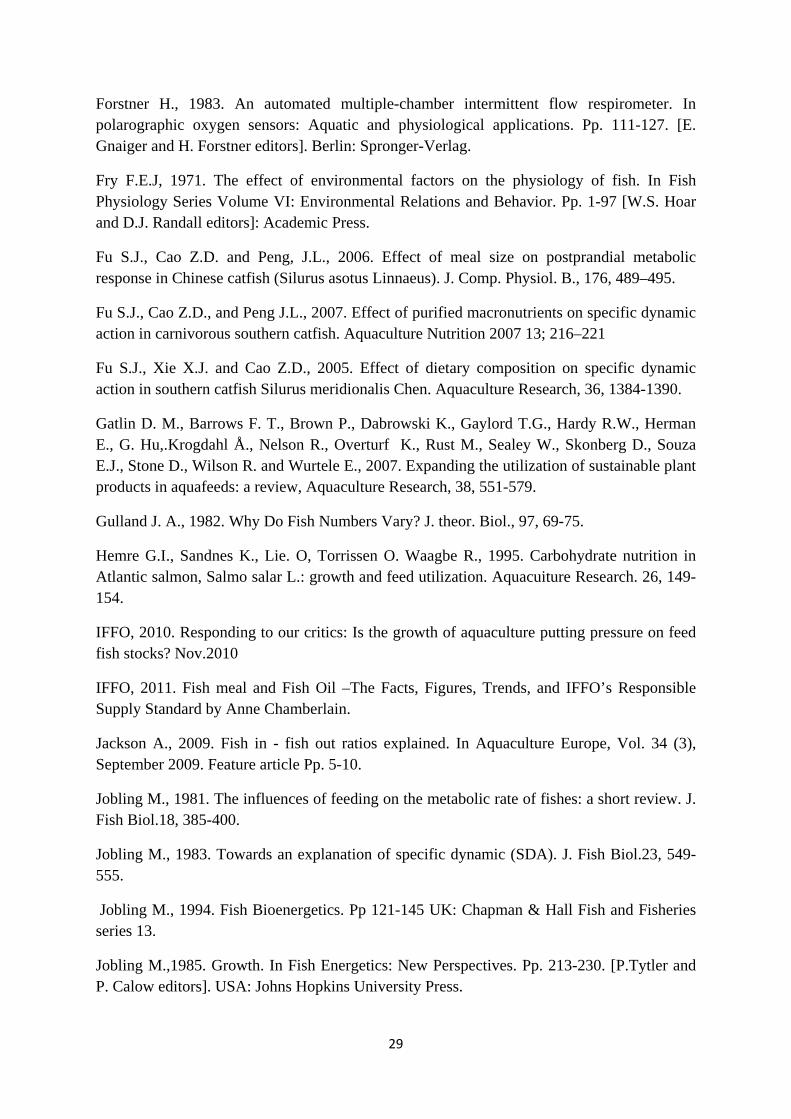
29

Forstner H., 1983. An automated multiple-chamber intermittent flow respirometer. In polarographic oxygen sensors: Aquatic and physiological applications. Pp. 111-127. [E. Gnaiger and H. Forstner editors]. Berlin: Spronger-Verlag.

Fry F.E.J, 1971. The effect of environmental factors on the physiology of fish. In Fish Physiology Series Volume VI: Environmental Relations and Behavior. Pp. 1-97 [W.S. Hoar and D.J. Randall editors]: Academic Press.

Fu S.J., Cao Z.D. and Peng, J.L., 2006. Effect of meal size on postprandial metabolic response in Chinese catfish (Silurus asotus Linnaeus). J. Comp. Physiol. B., 176, 489–495.

Fu S.J., Cao Z.D., and Peng J.L., 2007. Effect of purified macronutrients on specific dynamic action in carnivorous southern catfish. Aquaculture Nutrition 2007 13; 216–221

Fu S.J., Xie X.J. and Cao Z.D., 2005. Effect of dietary composition on specific dynamic action in southern catfish Silurus meridionalis Chen. Aquaculture Research, 36, 1384-1390.

Gatlin D. M., Barrows F. T., Brown P., Dabrowski K., Gaylord T.G., Hardy R.W., Herman E., G. Hu,.Krogdahl Å., Nelson R., Overturf K., Rust M., Sealey W., Skonberg D., Souza E.J., Stone D., Wilson R. and Wurtele E., 2007. Expanding the utilization of sustainable plant products in aquafeeds: a review, Aquaculture Research, 38, 551-579.

Gulland J. A., 1982. Why Do Fish Numbers Vary? J. theor. Biol., 97, 69-75.

Hemre G.I., Sandnes K., Lie. O, Torrissen O. Waagbe R., 1995. Carbohydrate nutrition in Atlantic salmon, Salmo salar L.: growth and feed utilization. Aquacuiture Research. 26, 149-154.

IFFO, 2010. Responding to our critics: Is the growth of aquaculture putting pressure on feed fish stocks? Nov.2010

IFFO, 2011. Fish meal and Fish Oil –The Facts, Figures, Trends, and IFFO’s Responsible Supply Standard by Anne Chamberlain.

Jackson A., 2009. Fish in - fish out ratios explained. In Aquaculture Europe, Vol. 34 (3), September 2009. Feature article Pp. 5-10.

Jobling M., 1981. The influences of feeding on the metabolic rate of fishes: a short review. J. Fish Biol.18, 385-400.

Jobling M., 1983. Towards an explanation of specific dynamic (SDA). J. Fish Biol.23, 549-555.

Jobling M., 1994. Fish Bioenergetics. Pp 121-145 UK: Chapman & Hall Fish and Fisheries series 13.

Jobling M.,1985. Growth. In Fish Energetics: New Perspectives. Pp. 213-230. [P.Tytler and P. Calow editors]. USA: Johns Hopkins University Press.

30

Kerr S.R, 1971. Analysis of Laboratory Experiments on Growth Efficiency of Fishes. Fisheries Research Board of Canada., Vol.28, NO.6.

Leeuwen T.E.V., Rosenfeld J. S., and Richards J. G., 2012. Effects of food ration on SMR: influence of food consumption on individual variation in metabolic rate in juvenile coho salmon (Onchorhynchus kisutch). Journal of Animal Ecology, 81, 395–402.

Lucas A., 1992. Bioenergetics of Aquatic Animals, [I.G. Priede, editor of English edition, 1996], Taylor & Francis e-Library, 2002.

Luo Y. and Xie X. 2008; Effects of temperature on the specific dynamic action of the southern catfish, Silurus meridionalis Comp. Bioch. and Physiol., Part A 149, 150–156.

Luo Y. and Xie X. 2009. The effect of temperature on post-feeding ammonia excretion and oxygen consumption in the southern catfish. J Comp. Physiol. Part B, 179, 681–689.

McCue M.D., 2006. Specific dynamic action: A century of investigation-Review. Comp. Bioch. and Physiol., Part A, 144, 381–394.

Medland T.E. and Beamish F.W.H, 1985. The influence of diet and fish density on apparent heat Increment in rainbow trout, salmo gairdneri. Aquaculture, 47, l-10.

Millidine K.J., Armstrong J.D., and Metcalfe N.B., 2009. Juvenile salmon with high standard metabolic rates have higher energy costs but can process meals faster. Proc. R. Soc. B., 276, 2103-2108.

Mitchell M.M., 1962. Comparative nutrition of man and domestic animals Vol.II. Pp. 3-82. Academic Press.

Nelson J.A. & Chaboat D., 2011. General energy metabolism. In encyclopedia of fish physiology: from genome to environment Vol.III.Pp 1566-1572 [A. P. Farrell editor]. Academic Press.

Noble R. L., 1973. Evacuation Rates of Young Yellow Perch, Perca flavescens, Transactions of the American Fisheries Society, 102,4, 759-763

Owen SF., Houlihan D.F., Rennie M.J., van Weerd J.H,.1998. Bioenergetics and ammonia balance of the European eel (Anguilla anguilla) fed at high and low ration levels. Can J Fish Aquat Sci 55, Pp. 2365–2375

Pang X., Cao Z.D., and Fu S.J., 2010. The effects of temperature on metabolic interaction between digestion and locomotion in juveniles of three cyprinid fish (Carassius auratus, Cyprinus carpio and Spinibarbus sinensis) Comp. Bioch. and Physiol., Part A 159, 253–260.

Preez H. H. D.U., Strydom W., and Winter P. E. D., 1986. Oxygen consumption of two marine teleosts, lithognathus mormyrus (linnaeus, 1758) and lithognathus lithognathus (cuvier, 1830) (teleosti: sparidae) Camp. Biochem. Physiol. 85A, No. 2, 313-331, 1986.

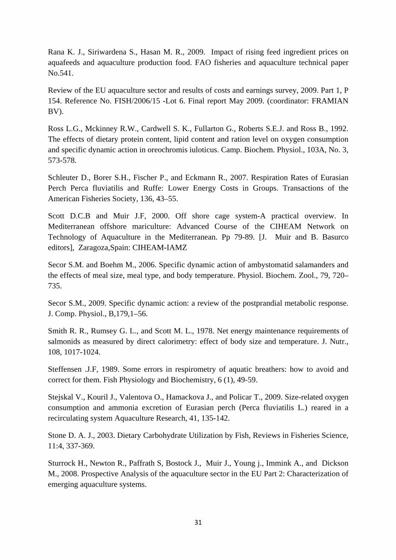
31

Rana K. J., Siriwardena S., Hasan M. R., 2009. Impact of rising feed ingredient prices on aquafeeds and aquaculture production food. FAO fisheries and aquaculture technical paper No.541.

Review of the EU aquaculture sector and results of costs and earnings survey, 2009. Part 1, P 154. Reference No. FISH/2006/15 -Lot 6. Final report May 2009. (coordinator: FRAMIAN BV).

Ross L.G., Mckinney R.W., Cardwell S. K., Fullarton G., Roberts S.E.J. and Ross B., 1992. The effects of dietary protein content, lipid content and ration level on oxygen consumption and specific dynamic action in oreochromis iuloticus. Camp. Biochem. Physiol., 103A, No. 3, 573-578.

Schleuter D., Borer S.H., Fischer P., and Eckmann R., 2007. Respiration Rates of Eurasian Perch Perca fluviatilis and Ruffe: Lower Energy Costs in Groups. Transactions of the American Fisheries Society, 136, 43–55.

Scott D.C.B and Muir J.F, 2000. Off shore cage system-A practical overview. In Mediterranean offshore mariculture: Advanced Course of the CIHEAM Network on Technology of Aquaculture in the Mediterranean. Pp 79-89. [J. Muir and B. Basurco editors], Zaragoza,Spain: CIHEAM-IAMZ

Secor S.M. and Boehm M., 2006. Specific dynamic action of ambystomatid salamanders and the effects of meal size, meal type, and body temperature. Physiol. Biochem. Zool., 79, 720–735.

Secor S.M., 2009. Specific dynamic action: a review of the postprandial metabolic response. J. Comp. Physiol., B,179,1–56.

Smith R. R., Rumsey G. L., and Scott M. L., 1978. Net energy maintenance requirements of salmonids as measured by direct calorimetry: effect of body size and temperature. J. Nutr., 108, 1017-1024.

Steffensen .J.F, 1989. Some errors in respirometry of aquatic breathers: how to avoid and correct for them. Fish Physiology and Biochemistry, 6 (1), 49-59.

Stejskal V., Kouril J., Valentova O., Hamackova J., and Policar T., 2009. Size-related oxygen consumption and ammonia excretion of Eurasian perch (Perca fluviatilis L.) reared in a recirculating system Aquaculture Research, 41, 135-142.

Stone D. A. J., 2003. Dietary Carbohydrate Utilization by Fish, Reviews in Fisheries Science, 11:4, 337-369.

Sturrock H., Newton R., Paffrath S, Bostock J., Muir J., Young j., Immink A., and Dickson M., 2008. Prospective Analysis of the aquaculture sector in the EU Part 2: Characterization of emerging aquaculture systems.

32

Tacon A. G.J. and Metian M., 2008. Global overview on the use of fish meal and fish oil in industrially compounded aquafeeds: Trends and future prospects Aquaculture, 285, 146–158

Tidwell J. H., 2012. Characterization and Categories of Aquaculture Production Systems. In Aquaculture Production Systems. Pp 64-77. [J. Tidwell editor] Wiley-Blackwell

Tucker C. and Hargreaves J., 2012. Ponds. In Aquaculture Production Systems. Pp. 191-242. [J. Tidwell editor] Wiley-Blackwell.

Vanella F.A., Boy C. C., Lattuca M. E., and Calvo J., 2010. Temperature influence on post-prandial metabolic rate of sub-Antarctic teleost fish. Comp. Bioch. and Physiol., Part A 156, 247–254.

Voutilainen A., Seppänen E. and Huuskonen H., 2011. A methodological approach to measuring the oxygen consumption profile of six freshwater fish species: implications for determination of the standard metabolic rate. Marine and Freshwater Behaviour and Physiology, 44(4), 239-250.

Wang Q., Wang W., Huang Q., Zhang Y. and Luo Y., 2012. Effect of meal size on the specific dynamic action of the juvenile snakehead (Channa argus). Comp. Bioch. and Physiol., Part A 161, 401–405.

Weir J. B.V., 1949. New methods for calculating metabolic rate with special reference to protein metabolism. J. Physiol. 109, 1-9.

Werner, F. E., and Quinlan J. A., 2002. Fluctuations in marine fish populations: physical processes and numerical modelling. – ICES Marine Science Symposia, 215, 264–278.

Wiegert R.G.,1968. Thermodynamic considerations in animal nutrition. AM. Zoologist, 8, 71-81.

Wilson R.P., 1994. Utilization of dietary carbohydrate by fish-Review. Aquaculture 124, 67-80

Zakus´ Z., Zakus K. D., and Kata K., 2003. Rates of oxygen consumption and ammonia excretion of juvenile Eurasian perch Perca fluviatilis. Aquaculture International, 11, 277–288

Zimmermann1 C. and Kunzmann A., 2001; Baseline respiration and spontaneous activity of sluggish marine tropical fish of the family Scorpaenidae , Mar. Ecol. Prog. Ser., 219, 229–239.

33

Appendix

Table 1A Recirculation aquaculture productions (tons) of EU countries and change in production from 2000 to 2005 (Adapted from Sturrock et al., 2008). Country Production Change (%) Species produced

Czech Rep. <20a - European catfish, African catfish; Tilapia; Eel. Denmark 3300 - Eel; turbot fry Finland 300 200 Arctic charr; sturgeon

France - 50 Bass; bream; turbot; meagre; perch; trout; sturgeon; red drum.

Germany 830 - Eel; catfish; hybrid. sturgeon; Striped bass Greece ? - Eel Hungary 1000* small + African catfish; sturgeon Ireland <50 100 Arctic charr; codlings. perch; live rotifers; Codling

Italy 40 million fingerlings -100 Bass & bream fry

Netherlands 9220b see note Eel; sole; African catfish; tilapia; turbot; pike perch; koi carp; barramundi

Norway 1 million 100 Cod, salmon Poland 300 20 farms African catfish

Portugal ? 0 Bass, bream & turbot; and their fry

Spain Hatcheries Sweden 200 -60 Eel; perch. UK 575+ - Salmon smolts; turbot; tilapia; barramundi a only partial recirculation. b RAS is the dominant production system in Netherland. Note: -45% eels; -3% catfish; +25% turbot; +100% pike perch; 4 new tilapia farms. Sea bass, seabream and trout were the main species at fingerling levels. The major species produced at grow out level were eel, African catfish, and trout. The production by RAS was not ascending or stable in all the EU countries. Some countries had shown increased production by RAS, some had remained unchanged and some of them had a decrease in production. The reasons for decreased or unchanged production vary country to country. Some main reasons, however, are insufficient governmental support and funding, failure due to lack of knowledge and experts, no new established farm, and other technical problems. (Sturrock et al., 2008)

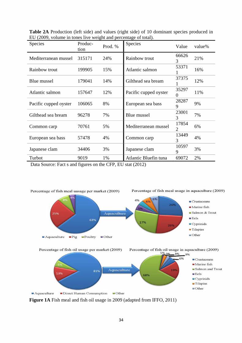
34

Table 2A Production (left side) and values (right side) of 10 dominant species produced in EU (2009, volume in tones live weight and percentage of total). Species Produc-

tion Prod. % Species Value value%

Mediterranean mussel 315171 24% Rainbow trout 666263 21%

Rainbow trout 199905 15% Atlantic salmon 533711 16%

Blue mussel 179041 14% Gilthead sea bream 373751 12%

Atlantic salmon 157647 12% Pacific cupped oyster 352970 11%

Pacific cupped oyster 106065 8% European sea bass 282879 9%

Gilthead sea bream 96278 7% Blue mussel 230013 7%

Common carp 70761 5% Mediterranean mussel 178542 6%

European sea bass 57478 4% Common carp 134493 4%

Japanese clam 34406 3% Japanese clam 105979 3%

Turbot 9019 1% Atlantic Bluefin tuna 69072 2% Data Source: Fact s and figures on the CFP, EU stat (2012)

Figure 1A Fish meal and fish oil usage in 2009 (adapted from IFFO, 2011)

35

Despite the fact that fish meal and fish oil are used in intensive livestock productions such as swine and poultry, aquaculture sector is the major consumer of these products. Recently, the high inclusion levels of fish meal and fish oil, particularly in diets of carnivore fish, has extensively called the attention. Shrimps, marine fishes, and salmons’ diets are formulated by high levels of fish meal. Table 3A Summary of FIFO Ratios as calculated by IFFO

Species FM in Dieta % FO in Dieta % EFCRb 2010

EFCRb

2020 FIFO Ratioac

Salmon 30 20 1.3 1.3 2.2 (1.68)d Trout 30 15 1.3 1.3 1.9 Eel 55 5 1.4 1.2 2.9 Marine Fish 32 8 1.8 1.7 1.9 Shrimp 20 2 1.6 1.4 1.2 FW Crustaceans 15 1.5 2.0 1.8 0.5 Tilapia 6 0.5 1.7 1.5 0.3 Catfish 10 1.7 1.5 1.3 0.4 Milk fish 3 1 2.0 1.7 0.1 Carp 5 0 1.7 1.5 0.1 Misc. FW Carn. Fishe 40 5 2.0 2.0 0.5 Pigs 0.25 0 - - 0.03 Poultry 0.30 0 - - 0.02 Aquaculture total 0.66 (0.52)d Note: Yield of fish meal (FM) from wild fish: 24%; yield of fish oil (FO) from wild fish: 5% a.Values from Jackson, 2009 b.EFCR: Estimated average species-group economic feed conversion ratio (total feed fed / total species-group biomass increase) for years 2010 and 2020; values from Tacon & Metian (2008). c.Values in the column were calculated without including the parts of FM and FO that originated from fisheries by-products. IFFO estimates that 22% of FM in 2008 derived from by-products rather than whole fish. ( )d FIFO ratio after inclusion of 22%. e.Miscellaneous Fresh Water Carnivore Fish.

Improved nutritional knowledge and feed conversion rate (FCR) have contributed to further reduction of fish meal usage. According to Jackson (2009), the technical director of IFFO, the current Fish in-fish out ratio (FIFO ratio= [level of fish meal in the diet + level fish oil in the diet] / [yield of fish meal from wild fish+ yield of fish oil from wild fish] ×FCR) for salmonids fish is 1.68 and for all aquaculture 0.52. It means that aquaculture industry produces around 1.92 tons of fish through every tone of whole-wild fish. FCR and thereby FIFO ratios are expected to improve further in the future. Alternative protein sources are also expected to replace part of fish meal in the diets. Whereas fish meal constituted 12.5% of total aquafeeds by weight in 2008, the portion is projected to reach 7.1 and 4.9% until 2015 and 2020, respectively (FAO, 2012). The FIFO ratio probably will decline further because the share of fish meal originated from fish processing residues is increasing along with aquaculture expansion. IFFO estimated that 22-25% of fish meal derived from fish trimming and residues in 2008. FAO (2012), states that the percentage hit 36% in 2010.

36

Figure 2A Commodity price of main protein and oil sources used in aquaculture (2004- 2009) (Rana et al., 2009).

Enhanced fuel costs and adverse climate conditions (e.g. drought in Russian Federation, Ukraine, Australia, South Africa, etc. in 2006-2007, and Brazil, Argentina, and Paraguay, 2008–2009) were the main commencer factors for the incident of price elevation. Moreover, it is worth bearing in mind that the prices of ingredients influence each other interactively according to supply and demand laws. Consider, for example, the sharp increase in price of fish meal in 2006 (figure 5). The reduction of landing due to quotas in Chili, Peru (on anchovy and jack mackerel.) and Scandinavia (on capelin, sand eel and blue whiting) couples with increased demand of fish meal from china for stockpiling this product, causing an abrupt increase in fish meal price. Subsequently, the price of soybean, wheat, and corn start to rise with comparatively greater rates during the next year, indicating both reduced production and increased demands for these products. The event can be perceived more distinctly through simultaneous increase in prices of fish oil, soybean oil, and rapeseed oil (the main substitute for fish oil in Europe) during 2007-2008 (Rana et al., 2009).

37

38

I denna serie publiceras examensarbeten (motsvarande 15, 30, 45 eller 60 högskolepoäng) vid Institutionen för husdjurens utfodring och vård, Sveriges lantbruksuniversitet. Institutionens examensarbeten finns publicerade på SLUs hemsida www.slu.se.

In this series Degree projects (corresponding 15, 30, 45 or 60 credits) at the Depart- ment of Animal Nutrition and Management, Swedish University of Agricultural Sciences, are published. The department's degree projects are published on the SLU website www.slu.se.

Sveriges lantbruksuniversitet

Fakulteten för veterinärmedicin och

husdjursvetenskap

Institutionen för husdjurens utfodring och vård

Box 7024

750 07 Uppsala

Tel. 018/67 10 00

Hemsida: www.slu.se/husdjur-utfodring-vard

Swedish University of Agricultural Sciences

Faculty of Veterinary Medicine and Animal Science

Department of Animal Nutrition and Management

PO Box 7024

SE-750 07 Uppsala

Phone +46 (0) 18 67 10 00

Homepage: www.slu.se/animal-nutrition-management