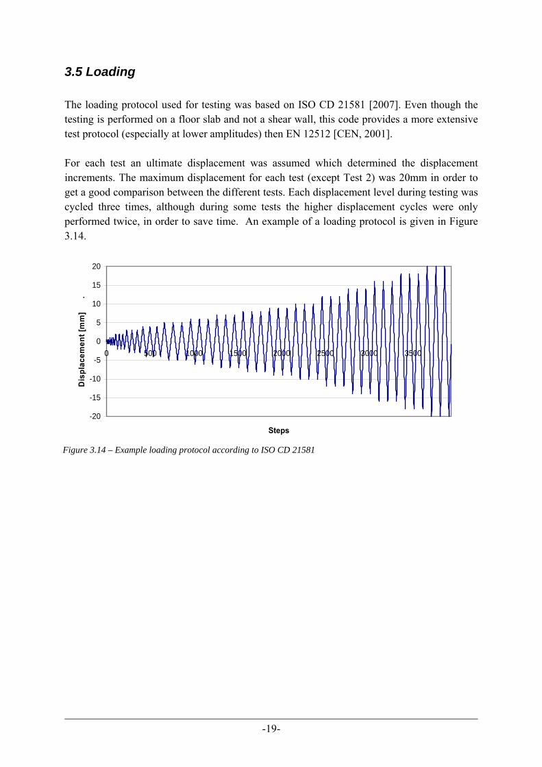
the effect of floor flexibility on the seismic behaviour...
TRANSCRIPT

Department of Civil and Natural Resources Engineering University of Canterbury & Faculty of Civil Engineering and Geosciences Delft University of Technology
The effect of floor flexibility on the seismic behaviour of post-tensioned timber buildings
Student: W.A. van Beerschoten Supervisors: Prof. A.H. Buchanan (UoC) Prof.ir. F.S.K. Bijlaard (TUD) Dr. ir. J.W.G. van de Kuilen (TUD)
Dr .ir. P.C.J. Hoogenboom (TUD) Ir. L.J.M. Houben (TUD) Advisors: D.M. Carradine (UoC) M.P. Newcombe (UoC) Date: 12 – May – 2009
This thesis is submitted in partial fulfilment of my Master Degree in Civil Engineering at Delft University of Technology in the Netherlands.

-i-
Acknowledgements I would like to thank Andy Buchanan for giving me the possibility to do my Master thesis at the University of Canterbury. It was a great opportunity for me to go to New Zealand and to do seven months of research in a new environment. Also the visit to several timber companies in Nelson and the opportunity to go to the New Zealand Society for Earthquake Engineering Conference is greatly appreciated. I would also like to thank Michael Newcombe for all the time he put in assisting me with my research. He did a great job in explaining the seismic engineering information which I lacked. He also designed the laboratory test setup which I could start using very soon after I started with my research. And he gave a lot of valuable feedback on the first versions of this report. The assistance I received from Gavin Keats and Russell McConchie with the experimental testing in the laboratory is greatly appreciated. The same holds for David Carradine, who assisted with the experimental testing and gave feedback on my report. I would like to acknowledge Stefano Pampanin for his input on the numerical analysis. He provided feedback on the first numerical calculations and gave valuable insight on the best way to present the results. Lastly, I would like to thank Jan-Willem van de Kuilen en Pierre Hoogenboom for taking part in my graduation committee and for the time they spend in reading and commenting on my reports.

-ii-
Summary This report describes the experimental testing on a timber-concrete composite floor to investigate the in-plane stiffness of the diaphragm and the stiffness and strength of different connections between the diaphragm and the lateral load resisting system. It also describes the numerical analysis, which investigates the effects of the floor flexibility on the seismic behaviour of post-tensioned timber buildings. The main objective is to get a better understanding of the influence of the floor flexibility on the seismic response of multi-story post-tensioned timber buildings. To evaluate the floor flexibility, a 1/3 scale test setup of a timber-concrete composite floor system has been constructed in the laboratory of the University of Canterbury. Seven tests with a different kind of connection between the floor and the lateral supports (which simulated the lateral load resisting system) have been performed. The experimental testing showed that there are major structural differences between the different connections which were tested. The timber-to-concrete connection with screws installed at a 45° angle was nearly twice as strong as the connection with screws at a 90° angle. For the timber-to-timber connections the orientation did not seem to influence the strength of the connection. The stiffness of screws installed at a 45° angle, 80 kN/mm, was four times larger than for screws at a 90° angle, 20 kN/mm. The displacement at maximum force was approximately 2 mm for the screws at a 45° angle, compared to 5 mm for the screws at a 90° angle and 14 mm for the nails. The tested diaphragm had an uncracked stiffness of 4000 kN/mm and a cracked stiffness of 300 kN/mm. For the tested floor unit it was concluded that the influence of the diaphragm flexibility was negligible compared to the connector flexibility. The floor flexibility can be idealized as three different parts, the deformation of the connectors, the shear deformation of the diaphragm and the flexural deformation of the diaphragm. The numerical analysis showed that it is not necessary to model the diaphragm as several beam elements; it is justified to model it as a single degree-of-freedom element. The influence of the floor flexibility on the seismic response of post-tensioned timber buildings is small. In most cases neglecting the floor flexibility is a conservative approach for the structural design of the building. Only for structures with a wall as lateral load resisting system and flexible connectors there can be an amplification of the seismic response. In that case it is sufficient to include only the flexibility of the connectors. It is recommended that the design spectral acceleration is used for the design of the connection between the floor diaphragm and the lateral load resisting system. This predicts the floor accelerations more accurately than a design using the peak ground acceleration

-iii-
Table of Contents
Glossary of Terms ...................................................................................................................... v
List of tables ............................................................................................................................... v
List of figures ............................................................................................................................ vi
1 Introduction ............................................................................................................................. 1 1.1 Background ...................................................................................................................... 1 1.2 Thesis statement ............................................................................................................... 1 1.3 Organisation ..................................................................................................................... 2
2 Literature study ....................................................................................................................... 3 2.1 Post-tensioned timber buildings ....................................................................................... 3 2.2 In-plane diaphragm stiffness and seismic response ......................................................... 4 2.3 Fasteners........................................................................................................................... 5 2.4 Building Standards ........................................................................................................... 5
3 Experimental testing.............................................................................................................. 10 3.1 Objectives....................................................................................................................... 10 3.2 Floor and test setup ........................................................................................................ 10 3.3 Materials......................................................................................................................... 13 3.4 Fasteners......................................................................................................................... 15 3.5 Loading........................................................................................................................... 18 3.6 Recycling........................................................................................................................ 20
4 Results experimental testing.................................................................................................. 21 4.1 Test 1 – Timber-to-concrete, screws, 90° ...................................................................... 21 4.2 Test 2 – Timber-to-concrete, screws, 45° ...................................................................... 22 4.3 Test 3 – Timber-to-timber, screws, 90°.......................................................................... 25 4.4 Test 4 – Timber-to-timber, nails, 90°............................................................................. 27 4.5 Test 5 – Timber-to-timber, screws, 45°.......................................................................... 29 4.6 Test 6 – Timber-to-timber, long screws, 90° ................................................................. 31 4.7 Test 7 – Diaphragm stiffness.......................................................................................... 33
5 Discussion and conclusions of experimental results ............................................................. 38 5.1 Connection strength........................................................................................................ 38 5.2 Connection stiffness ....................................................................................................... 39 5.3 Comparison between screws and nails........................................................................... 39 5.4 Comparison between thread and shank at connection interface..................................... 40 5.5 Diaphragm...................................................................................................................... 40 5.6 Conclusions .................................................................................................................... 42

-iv-
6 Numerical analysis of a floor unit ......................................................................................... 43 6.1 Introduction .................................................................................................................... 43 6.2 Numerical Model............................................................................................................ 43 6.3 Design Parameters.......................................................................................................... 45 6.4 Stiffness of the diaphragm.............................................................................................. 48 6.5 Floor mass ...................................................................................................................... 53 6.6 Design of the strength of the shear connectors............................................................... 54 6.7 Design of the stiffness of the shear connectors .............................................................. 56 6.8 Overview of Design Parameters..................................................................................... 59 6.9 Results ............................................................................................................................ 60 6.10 Comparison of the results............................................................................................. 66 6.11 Conclusions .................................................................................................................. 69
7 Numerical analysis of a single storey building ..................................................................... 70 7.1 Introduction .................................................................................................................... 70 7.2 Numerical Model............................................................................................................ 70 7.3 Design Parameters.......................................................................................................... 71 7.4 Stiffness of the LLRS..................................................................................................... 71 7.5 Results ............................................................................................................................ 74 7.6 Conclusions .................................................................................................................... 80
8 Numerical analysis of a multi-storey building ...................................................................... 81 8.1 Introduction .................................................................................................................... 81 8.2 Displacement Based Design........................................................................................... 82 8.3 Numerical Model............................................................................................................ 83 8.4 Design Parameters.......................................................................................................... 84 8.5 Results ............................................................................................................................ 85 8.6 Conclusions .................................................................................................................... 96
9 Conclusions ........................................................................................................................... 97
10 Recommendations for further research ............................................................................... 98
11 References ........................................................................................................................... 99
Appendix A – Calculations connection strength.................................................................... 103
Appendix B – Ruaumoko Frame Files ................................................................................... 111
Appendix C – Earthquake records ......................................................................................... 116
Appendix D – Graphs numerical analysis floor unit.............................................................. 119
Appendix E – Graphs numerical analysis multi-storey building ........................................... 124

-v-
Glossary of Terms DBD Displacement Based Design EC Eurocode FAM Floor Acceleration Magnification (=PFA/PGA) IBC International Building Code LLRS Lateral Load Resisting System LVL Laminated Veneer Lumber MDOF Multi Degree of Freedom PFA Peak Floor Acceleration PGA Peak Ground Acceleration SDOF Single Degree of Freedom TCC Timber Concrete Composite THA Time History Analysis
List of tables Table Title Page
3.1 Strength characteristic for Timber, Glulam and LVL [Buchanan, 2007] 14 3.2 Concrete mix [Le Heux, 2008] 14 3.3 Test results grout cylinders 15 3.4 Test results fastener testing 16 3.5 Test results from fastener bending 18 4.1 Overview of connections per test 21 4.2 Influence of the rope effect on the capacity 28 5.1 Overview of maximum strength for timber-to-concrete and timber-to-timber
connections 38
5.2 Influence of the diaphragm stiffness 41 6.1 Overview section properties 45 6.2 Fixed design parameters 46 6.3 Overview diaphragm stiffness 52 6.4 Overview floor mass 53 6.5 Overview connector forces 54 6.6 Strength of screwed connection for 6 different failure modes 55 6.7 Overview number of connectors 55 6.8 Overview of upper and lower values for the connector stiffness 58 6.9 Overview design parameters (1) 59 6.10 Overview design parameters (2) 59 8.1 Results DBD for 6 storey building 82 8.2 Overview of periods 92 9.1 Overview of how to the floor flexibility can be modelled 97

-vi-
List of figures Figure Title Page
2.1 Schematic contributions of connectors and diaphragm stiffness to the overall floor system stiffness [Brignola, 2008]
4
2.2 Explanation of flexible and rigid diaphragm 6 2.3 Different distributions of the base shear 9 3.1 Test setup in the laboratory 10 3.2 Details of test setup, c.o. Lorent (unpublished work) 11 3.3 Measurement instrumentation on the floor 12 3.4 LVL production [Buchanan, 2007] 13 3.5 Stack of LVL panels 13 3.6 Low variability of LVL [Buchanan, 2007] 13 3.7 Gap in the concrete which was filled with grout 14 3.8 Tested grout cylinders – on the left the failure in the compression test, right the
failure in the splitting test 15
3.9 Schematic test setup [ASTM, 2003] 15 3.10 Photo of fastener testing 15 3.11 Three different loading positions for fastener testing 16 3.12 Load displacement graphs of fastener testing 17 3.13 Normal distributions of the fasteners (vertical axis is scaled for better graph) 18 3.14 Example loading protocol according to ISO CD 21581 19 3.15 Recycling of the floor (clockwise: metal fasteners and brackets, LVL, plywood
and concrete) 20
4.1 Double yielding in the fastener [Le Heux, 2008] 21 4.2 Hysteresis loops Test 1 [Le Heux, 2008] 22 4.3 Timber-to-concrete connection with screws under a 45° angle 22 4.4 Failure mode III [Kavaliauskas, 2007] 23 4.5 Failure in the grout 23 4.6 Connection displacement for Test 2 24 4.7 Hysteresis loops Test 2, 4 graphs with each three series of three displacement
cycles 24
4.8 Hysteresis loops Test 2 25 4.9 Connection Test 3 26
4.10 Six failure modes according to EC5 [CEN, 2004b] 26 4.11 Failure of the fastener 27 4.12 Hysteresis loops Test 3 27 4.13 Hysteresis loops Test 4 28 4.14 Hysteresis loops Test 5 29 4.15 Failure in the timber frame and the screw still fixed to the joist 30 4.16 Hysteresis loops and friction loop Test 5 30 4.17 Hysteresis loops Test 6 31 4.18 Hysteresis loops and friction loop Test 6 32

-vii-
4.19 Steel angles to fix the floor diaphragm 33 4.20 Hysteresis loops of the whole system 34 4.21 Hysteresis loops of the connection 34 4.22 Hysteresis loops and stiffness of the diaphragm 35 4.23 Stiffness comparison of the diaphragm, the connection and the reaction frame 35 4.24 Displacement of the diaphragm 36 4.25 Cracking of the concrete 36 4.26 Complete cracking pattern in the concrete 37 5.1 Comparison between the maximum strength for the timber-to-concrete and
timber-to-timber connections 38
5.2 Comparison between the stiffness for the timber-to-concrete and timber-to-timber connections
39
5.3 Comparison between screws and nails as connectors 39 5.4 Comparison between fasteners with the thread and shank at the interface of the
connection 40
6.1 Three floor deformation components 43 6.2 Three numerical models 44 6.3 Five designs with different aspect ratios 45 6.4 Schematics of the calculations of the diaphragm stiffness 46 6.5 Schematics of the calculations of the period of the connection 47 6.6 Beam model of the diaphragm for determining the flexural stiffness 48 6.7 Comparison of the deflection under three different loading configurations 49 6.8 Beam model of the diaphragm for determining the shear stiffness 49 6.9 Experimental stiffness of the diaphragm 51
6.10 Idealization of the floor diaphragm for numerical models 52 6.11 Double yielding of fastener 56 6.12 Comparing Design E with the complex model 61 6.13 Displacements of Design E calculated with the complex model 61 6.14 Specification of the design range 62 6.15 Comparison of the floor displacement between the MDOF model and the SDOF
models 62
6.16 PFA distribution over the floor 63 6.17 Explanation of processing the floor accelerations 64 6.18 Spectral acceleration graph 64 6.19 Comparison of the earthquake acceleration and two different floor vibrations 65 6.20 Comparison of the earthquake acceleration with the floor acceleration 65 6.21 Comparison of floor displacements of the MDOF model and SDOF-1 model 66 6.22 Comparison of floor displacements of the MDOF model and SDOF-2 model 66 6.23 Diaphragm displacement according to the MDOF model 67 6.24 Comparison of peak floor acceleration between the MDOF model and SDOF-1
model 67
6.25 Comparison of peak floor acceleration between MDOF model and SDOF-2 model
68

-viii-
6.26 PFA / PGA according to the MDOF model 68 7.1 The four numerical models 70 7.2 Single storey building with frame 71 7.3 Equations for the target displacement, effective mass and effective height 71 7.4 The 5% and the scaled displacement spectrum 72 7.5 The 5% and the scaled displacement spectrum 72 7.6 Displacements of single storey building with frame as LLRS according to the
complex model 74
7.7 Comparison of floor displacements of single storey building with frame as LLRS 75 7.8 Further comparison of displacements of single storey building with frame as
LLRS 75
7.9 Comparison of floor accelerations of single storey building with frame as LLRS 75 7.10 Comparison of Median shear force of single storey building with frame as LLRS 76 7.11 Displacements of single storey building with wall as LLRS according to the
complex model 77
7.12 Comparison of floor displacements of single storey building with wall as LLRS 77 7.13 Further comparison of displacements of single storey building with wall as LLRS 77 7.14 Comparison diaphragm flexibility with different code requirements 78 7.15 Comparison of floor accelerations of single storey building with wall as LLRS 79 7.16 Spectral acceleration graph 79 7.17 Comparison of median shear force of single storey building with wall as LLRS 79 8.1 6 Storey building, artist impression, typical floor plan and connection detail
[Newcombe, 2008b; Smith, 2008] 81
8.2 Spectral acceleration for DBD 82 8.3 6 Storey building model with rigid floor and flexible floor assumption 83 8.4 Typical sections of beams and columns 83 8.5 Hysteresis loops used to model the properties of the connectors 84 8.6 Derivation of the deflections (u) and inter-storey drift levels (D) for the 6 storey
building 85
8.7 Frame deflections at three different earthquake intensities for the 6 storey building
85
8.8 Frame deflections of the 6 stories under the third earthquake record 86 8.9 Inter-storey drifts at three limit states for the 6 storey building 86
8.10 Derivation of the shear force and bending moments for the 6 storey building 87
8.11 Comparison of shear forces for the 6 storey building 88 8.12 Comparison of bending moments for the 6 storey building 88 8.13 Peak floor acceleration over the peak ground acceleration for the 6 storey
building 89
8.14 Connector displacement at top floor under the third earthquake record 90 8.15 Hysteresis loops of the connector at top level under the third earthquake record 90 8.16 Connector displacement vs. Connector Force for 1/50 year earthquake 91 8.17 Connector displacement vs. Connector Force for 1/500 year earthquake 91 8.18 Connector displacement vs. Connector Force for 1/2500 year earthquake 91

-ix-
8.19 Floor acceleration spectra at the levels 1 & 2, 3 & 4 and 5 & 6 of the building 93 8.20 Three normal modes of vibration 94 8.21 Floor acceleration magnifications 94
-1-
1 Introduction This report describes the experimental testing on a timber-concrete composite floor to investigate the in-plane stiffness of the diaphragm and the stiffness and strength of different connectors between the diaphragm and the lateral load resisting system. It also describes the numerical analysis, which used the data from the experimental testing. This numerical analysis investigates the effects of the floor flexibility on the seismic behaviour of post-tensioned timber buildings.
1.1 Background Recently there has been renewed interest in multi-storey timber buildings within New Zealand [Newcombe, 2008a]. This has lead to a large research program at the University of Canterbury. Researchers are currently working on a project to produce structural design and construction guidelines for post-tensioned multi-storey timber buildings. One of the components of interest is the in-plane stiffness of the floor and the connection between the floor diaphragm and the lateral load resisting system (LLRS). Many researchers have focused their attention on the field of diaphragm flexibility and the influence of flexible diaphragms on the seismic response of multi-storey buildings. Most of these studies focus on concrete buildings. In this report the effects of the diaphragm flexibility have been evaluated for the newly developed post-tensioned timber building system.
1.2 Thesis statement The main objective is to investigate the influence of the floor flexibility on the seismic response of post-tensioned timber buildings. It might be that the floor flexibility reduces the seismic response, or it might cause vibrations which amplify the seismic response. In order to evaluate the floor flexibility, a 1/3 scale test setup of a timber-concrete composite (TCC) floor system has been constructed in the laboratory. The goal of the experimental testing is to acquire data about the strength and stiffness of different connectors between the floor diaphragm and the LLRS. Also the in-plane stiffness of the diaphragm will be investigated. A numerical analysis will be performed in order to describe the parameters that influence the floor response, to determine how the floor flexibility can be modelled and to investigate the influence of floor flexibility in real structures. Once an accurate model for the floor is developed, the model will be extended with the LLRS to get a better understanding of the

-2-
interaction between the floor diaphragm and the LLRS. The last step will be to investigate the seismic response of a six storey building.
1.3 Organisation Chapter two gives a literature review about the development of post-tensioned timber buildings in New Zealand. It also gives an overview of other research performed on diaphragm stiffness and the strength of different types of fasteners. It concludes with a summary of diaphragm design information from different building codes. The third chapter describes the test setup for the experimental testing. It reviews the materials which are used, the fasteners and their characteristics, the loading procedure and the recycling of the floor after the test. The forth chapter gives an overview of the seven tests performed and the results of these tests. The test results are evaluated in chapter five. Chapter six is the start of the numerical analysis. This chapter describes the models which are made to investigate the different deformation components of the floor. In chapter seven the lateral load resisting system is added to the models to model a single-storey building. In chapter eight a detailed analysis of a six storey building is described.

-3-
2 Literature study This literature review is divided into four parts. The first part describes how this research report fits in the framework of research projects currently ongoing at the University of Canterbury. The second part clarifies the current state of research on diaphragm stiffness and its influence on the seismic response of multi-storey buildings. Part three gives an overview of three papers used in the design of the connections. Part four gives an overview of information about diaphragm design in different building standards.
2.1 Post-tensioned timber buildings New forms of multi-storey timber buildings are being developed at the University of Canterbury. An extensive experimental program focuses on structural systems using laminated veneer lumber (LVL) [Palermo et al., 2005]. The first stage of the research program focussed on the conceptual development, design details, construction and experimental tests. The second stage will focus on the global seismic performance of hybrid LVL systems. In the third and final stage, issues related to the effects of the floor diaphragm will be investigated. One of the main aspects in the new structural system is the use of post-tensioned timber members for both frame and wall systems [Palermo et al., 2006]. The post-tensioning, together with energy dissipaters, creates a ‘hybrid’ system which results in simple moment resisting connection. These connections have an energy dissipation and self-centring capacity. This system gives the opportunity to create large open spaces and provide a good resistance to earthquakes. This gives them the potential to compete with concrete or steel structures within New Zealand [Smith, 2008]. Another key aspect is the floor system. The timber-concrete composite (TCC) floor system is most viable for multi-storey buildings due to its low weight, good acoustic performance and limited deflections at larger spans [Buchanan et al., 2008]. A lot of research has focussed on the timber-to-concrete connections in order to achieve a high degree of composite action [Deam, 2007; Linden, 1999; Lukaszewska, 2007; Seibold, 2004]. So far the effect of the in-plane diaphragm stiffness on the seismic response of multi-storey timber buildings has had little attention. Le Heux [2008] showed that for TCC floor systems the stiffness of the diaphragm is much larger than the stiffness of the connection between the lateral load resisting system (LLRS) and the floor unit. The latter is therefore a major focal point in the experimental part of this report.

-4-
2.2 In-plane diaphragm stiffness and seismic response Diaphragm flexibility has been a topic on which a lot of researchers have focussed their attention. Several studies concluded that building codes and design standards underestimate the diaphragm design forces and that precast concrete floor systems can be quite flexible [Fleischman and Farrow, 2001; Iverson and Hawkins, 1994; Lee et al., 2007]. Fleischman and Farrow [2001] showed that long-span precast concrete diaphragms can be highly flexible when compared to the LLRS. This can lead to increased diaphragm forces and non-ductile diaphragm failure or structural instability due to high drift demands in the gravity system. They conclude that current design procedures based on rigid diaphragms are not adequate to predict the seismic demands on structures with flexible diaphragms. It is likely that long span TCC floors will be similarly flexible. Studies of the stiffness of concrete diaphragms [Lee et al., 2007; Nakaki, 2000] have mainly focussed on the stiffness of precast concrete elements with discrete connectors. An overall effective flexural stiffness is used that takes into account cracking of the concrete and deformation of the discrete connections between floor units. While for some types of concrete diaphragms this may be reasonable, for TCC floor units it is possible that the most significant deformation component comes from the discrete connectors between the LLRS and the diaphragm. If this is the case, the structural response of the floor could be simplified to a single degree of freedom (SDOF) system. This would have implications for the expected peak floor accelerations and displacements during an earthquake. In TCC-floors, the stiffness is a combination of the flexural and shear deformation of the floor unit and the deformation of the connectors between the floor unit and the LLRS [Brignola, 2008]. She proposed to model the diaphragm and the connector stiffness as shown in Figure 2.1. This way of modelling excludes the possibility of higher modes of response from the combination of the two different elements.
Figure 2.1 – Schematic contributions of connectors and diaphragm stiffness to the overall floor system stiffness [Brignola, 2008]

-5-
2.3 Fasteners Johansen’s yield theory is widely used to calculate the load carrying capacity of timber-to-timber and timber-to-steel connections [CEN, 2004b]. Dias [2005] showed that the formulas from EC5 are also applicable to concrete-to-timber connections. The theory of Johansen’s yield theory has been expanded to inclined screws in timber-to-timber connections [Bejtka, 2002] and for inclined screws in concrete-to-timber connections [Kavaliauskas, 2007]. All of these studies only focus on uni-directional loading, not on cyclic loading, as will be the case under earthquake loading.
2.4 Building Standards This section gives an overview of the sections from the New Zealand standard [1993; 2004; 2006] and the Eurocode [CEN, 2004b; CEN, 2004c; CEN, 2004d] relevant for this report. In literature often references to the IBC [International Code Council., 2003] can be found, therefore this is included in some parts of this chapter. In general it can be noted that there is a lack of design guidelines for diaphragms in TCC floors and for the design of the connection between the TCC floor and a timber LLRS.
2.4.1 Diaphragm stiffness
For the ease of the design process, diaphragms are classified as rigid or flexible. This is done in the following way by the three standards.
NZ1170.5 Rigid diaphragm: A diaphragm that is sufficiently rigid that the maximum lateral deflection is less than twice the average inter-storey deflection at that level.
EC8 The diaphragm is taken as being rigid, if, when it is modelled with its actual in-plane flexibility, its horizontal displacements nowhere exceed those resulting from the rigid diaphragm assumption by more than 10% of the corresponding absolute horizontal displacements in the seismic design situation.
IBC A diaphragm is rigid for the purpose of distribution of story shear and torsional moment when the lateral deformation of the diaphragm is less than or equal to two times the average story drift.
These definitions are explained with the help of Figure 2.2. The average inter-storey drift (or for a single storey building, the total horizontal displacement) is ullrs. The horizontal deflection of the diaphragm is ufloor. The New Zealand standard and the IBC require for a rigid diaphragm that:

-6-
ufloor + ullrs ≤ 2 x ullrs or ufloor ≤ ullrs. EC8 requires that: ufloor ≤ 10% x ullrs. It can be seen that there is a factor ten difference between the two standards.
2.4.2 Diaphragm design
Eurocode 8 [CEN, 2004d] gives several design rules for (concrete) diaphragms. A short overview is presented below.
4.2.1.5.(2) Floor systems and the roof should be provided with in-plane stiffness and resistance and with effective connection to the vertical structural system.
4.3.1.(7) Unless a more accurate analysis of the cracked element is performed, the elastic flexural and shear stiffness properties of concrete and masonry elements may be taken to be equal to one-half of the corresponding stiffness of the uncracked elements.
4.4.2.5.(1) Diaphragms and bracings in horizontal planes shall be able to transmit, with sufficient overstrength, the effects of the design seismic action to the lateral load-resisting system […].
4.4.2.5.(2) The recommended value [for γd (overstrength)] for brittle failure modes, such as shear in concrete diaphragms is 1.3.
5.10.(1) A solid reinforced concrete slab may be considered to serve as a diaphragm, if it has a thickness of not less than 70 mm […].
Figure 2.2 – Explanation of flexible and rigid diaphragm
ullrs ullrs
ufloor

-7-
5.10.(4) Action-effects in reinforced concrete diaphragms may be estimated by modelling the diaphragm as a deep beam […].
Section 4.2.1.5.(2) mentions an ‘effective connection’, but what characteristics result in an effective connection is not mentioned. In this report there are several different connections analysed and compared. Section 4.3.1.(7) gives a reduction factor of 0.5 for the stiffness of a cracked concrete diaphragm. Eurocode 5 [CEN, 2004c] states the following:
5.2.(5) [...] As a simple approach the stiffness of the cracked part of the concrete cross-section may be taken as 40% of the stiffness in un-cracked condition.
The determination of the stiffness of the diaphragm is part of the experimental testing and the results will be used to check the validity of these factors, which is presented in Section 5.5 and Section 6.4. The New Zealand standard for earthquake loading [Standards New Zealand, 2004] provides the following information about floor diaphragms:
6.1.4.1 For structures over 15 m in height where the structure is classified as irregular […], diaphragms shall be modelled in a three-dimensional model response spectrum or three-dimensional numerical integration time history analysis. Where diaphragms are not rigid compared to the vertical elements of the vertical action resisting system, the model should include representation of the diaphragm’s flexibility.
6.1.4.2 Actions within the diaphragm shall account for higher mode effects and the influence of overstrength actions […].
Section 6.1.4.1 raises the question how to model the diaphragm’s flexibility. This is evaluated in Chapter 6. In the New Zealand standard for Timber Structures [Standards New Zealand, 1993] only covers the design for diaphragms consisting of wood passed panels. As mentioned before, in the design of multi-storey timber buildings the most likely floor system will be a TCC floor. The diaphragm design of this floor system is not covered by the timber standard. The New Zealand concrete standard [Standards New Zealand, 2006] does cover the diaphragm design, but the connection between the diaphragm and the LLRS is less than adequate.
13.3.7.5 Connections by means of reinforcement from precast or cast-in-place concrete diaphragms to components of the primary force-resisting systems shall be adequate to accommodate the expected deformations at the interface while maintaining load paths.

-8-
No connection by means of reinforcement is possible between the TCC floor and a timber frame or wall. Several possible connections are described in Chapter 4.
2.4.3 Earthquake loading
The New Zealand standard and the EC8 have a similar way describing the earthquake response of structures. Both allow for non-linear methods (e.g. time-history analysis) or linear-elastic methods for regular buildings. For the latter an elastic response spectrum is made on the basis of several parameters belonging to the location and type of the building. This spectrum results in an acceleration, which multiplied by the effective mass of the building gives the design base shear. The base shear is distributed to the different floor levels of the building. The New Zealand standard, NZ1170.5, gives the following formula.
6.2.1.3 The equivalent static horizontal force Fi at each level, i, shall be obtained from:
1
0.92( )
where 0.08 at the top level and zero elsewhere.
i ii t n
i ii
t
W hF F VW h
F V=
×= + ×
×
=
∑
[V is the base shear]
EC8 allows for two different ways of distributing the base shear.
4.3.3.2.3(1) The fundamental mode shapes in the horizontal directions of analysis of the building may be calculated using methods of structural dynamics or may be approximated by horizontal displacements increasing linearly along the height of the building.
4.3.3.2.3(2) The seismic action effects shall be determined by applying, to the two planar models, horizontal forces Fi to all storeys.
i ii b
j j
s mF Fs m×
= ××∑
where: Fi is the horizontal force acting on storey I; Fb is the seismic base shear […]; si, sj are the displacements of masses mi, mj in the fundamental mode shape; mi, mj are the storey masses […].
4.3.3.2.3(3) When the fundamental mode shape is approximated by horizontal displacements increasing linearly along the height, the horizontal forces Fi should be taken as being given by:

-9-
i ii b
j j
z mF Fz m×
= ××∑
where: zi, zj = the heights of the masses mi, mj above the level of application of the seismic action (foundation or top of a rigid basement).
4.3.3.2.3(4) The horizontal forces Fi determined in accordance with this clause shall be distributed to the lateral load resisting system assuming the floors are rigid in their plane.
Figure 2.2 shows the different distributions of the base shear force for a six storey building, with the same weight at each floor.
This research fits within the framework of research projects currently ongoing at the University of Canterbury. And although a lot of information is available about diaphragm flexibility, the focus on TCC floors and post-tensioned buildings is a new aspect. The connection between the diaphragm and the LLRS is often neglected in the design or simplified as a part of the floor diaphragm. But for TCC floors this connection might be an essential part in the floor flexibility. Further, it is noticed that for some parts of the diaphragm design, there is a lack of information in the building codes.
Figure 2.3 – Different distributions of the base shear

-10-
3 Experimental testing This chapter describes the objectives of the test, the layout of the TCC floor, the test setup and the materials used. An overview is given of the testing of the fasteners which were used. Also described are the loading procedure and the recycling of the floor after the test.
3.1 Objectives The main objective of the experimental testing is to acquire data about the strength and stiffness of different connectors between the floor diaphragm and the LLRS. Also the in-plane stiffness of the diaphragm will be investigated. To evaluate the floor flexibility a 1/3 scale test setup of a TCC floor system was designed according to Yeoh et al [2008] and has been constructed in the laboratory. This floor was subjected to 7 tests, each with a different connection, which are described in Chapter 4.
3.2 Floor and test setup A 3 x 3 m TCC floor system has been constructed in the structural testing laboratory of the Department of Civil and Natural Resources Engineering at University of Canterbury. This setup can be seen in Figure 3.1. The floor consisted of 7 LVL joists (45 x 150 mm) and a 25 mm concrete layer. Notched connections made sure that there was a good composite action between the joists and the concrete layer. The joists were connected to two transverse LVL beams with steel joist hangers. The transverse beams were supported at each end by a corbel. On each side of the floor a LVL beam represented the LLRS. This beam was connected to the steel reaction frame by four threaded bars, which were epoxyed into the timber and bolted to the steel frame. Some movement in this connection was possible due to oversize holes in the steel frame. This affected the rigidity of the whole setup, which influenced the last test.
Figure 3.1 – Test setup in the laboratory

-11-
In Figure 3.2 various details of the test setup can be seen. The gap between the outer joist and the LLRS was filled with an LVL packer, which was glued to the joist (see also Figure 4.9). This has been done in order to test additional timber-to-timber connections without a gap. Calculations showed that the timber-to-timber connections with the gap would have been too weak to be realistic.
Figure 3.3 shows the instrumentation utilized to monitor displacements on the floor. Five linear pots, 50mm travel and 5000 steps, were attached to a rectangular hollow section (RHS) section, which spanned across the floor and was attached to the floor with silicon only near the edges of the diaphragm. These pots were used to measure the deflection of the diaphragm. Two pots were attached along each edge of the floor and to the LLRS. They were used to measure the displacement of the connections. Two more pots were connected to the steel reaction frame in order to measure the displacement between the LLRS and the reaction frame. This data was used to get an indication for the displacement of the reaction frame. At one end a 250 kN ram was connected to the floor. Four threaded bars made it possible to apply the cyclic loading to the floor. At one end a load cell measured the force acting on the floor, at the other end a rotary pot was connected to control the displacement (the tests were displacement based). A positive displacement was extension of the rotary pot, which meant a pulling force in the ram, so movement of the floor towards the west.
Figure 3.2 –Details of test setup, c.o. Lorent (unpublished work)

-12-
Figure 3.3 –Measurement instrumentation on the floor

-13-
3.3 Materials
3.3.1 Laminated Veneer Lumber
Laminated Veneer Lumber (LVL) is a wood product made from rotary peeled veneers, which are glued and laid upon each other with parallel grain orientation (although cross banded is also possible) to form long continuous sections [Buchanan, 2007]. This process is shown in Figure 3.4; the result can be seen in Figure 3.5.
In New Zealand, LVL is mainly made from Radiata Pine. The main advantage of LVL is that it has a higher structural strength then the original solid timber. This is because the density, fibre strength and any defects (such as knots) are distributed to a point where they do not influence the structural properties. This results in a lower variability, as can be seen from Figure 3.6. This graph shows the probability density function for the modulus of elasticity of machine graded timber and two LVL products. The solid vertical lines give the target average E-values and the dotted vertical line gives the 5th percentile E-value for the machine graded timber.
Figure 3.5 – Stack of LVL panels Figure 3.4 – LVL production [Buchanan, 2007]
Figure 3.6 – Low variability of LVL [Buchanan, 2007]

-14-
Table 3.1 shows an overview of the different strength characteristics of LVL, produced by Carter Holt Harvey and Nelson Pine, in comparison with sawn timber and glue laminated (glulam) timber.
3.3.2 Concrete
The constructed floor had a 25 mm thick concrete layer. The concrete consists of the components shown in Table 3.2 and was manufactured by J. Mackechnie. After 28 days the test cylinders reached a compressive strength of 24 MPa. The day that the first test took place, the strength was around 36 MPa. A fine steel wire mesh was used as reinforcement.
per 1m3 per 80 L Cement 280 22.4 kg Water 150 12 kg 6mm aggregate 1050 84 kg Sand 900 72 kg RMCO1 1800 144 mL Control 40 5000 400 mL
3.3.3 Grout
After the first test some of the concrete had to be taken out in order to make a different connection between the concrete layer and the timber frame, as can be seen in Figure 3.7. Grout has been used to fill this gap after the connection was made. This was done to not have to wait for a month for the concrete to cure. The grout used was “Sika Grout GP”, a high strength, shrinkage compensated, pourable cementitious grout [Sika Ltd, 2008]. Four test cylinders (Ø50 mm, 100 mm high)
Table 3.1 – Strength characteristic for Timber, Glulam and LVL [Buchanan, 2007]
Table 3.2 – Concrete mix [Le Heux, 2008]
Figure 3.7 – Gap in the concrete which was filled with grout

-15-
were made and tested at the day of the test, which was 12 days after the casting. Two cylinders were tested for compressive strength and two for tensile strength, by performing a splitting test. The results can be seen in Table 3.3. Figure 3.8 shows the tested cylinders.
Test Force [kN]
Strength [MPa]
Compression 1 93 47 Compression 2 110 56
Split 1 30 3.8 Split 2 45 5.7
3.4 Fasteners Six different types of fasteners have been used for the testing, five different types of screws and one type of nails. No specifications were available so the ASTM F 1575-03 [2003] was used to obtain the bending strength of the fasteners. These tests were performed after the floor testing, due to time constraints in the lab. Therefore the results of these tests are used as an evaluation of the test results, but not as a prediction of the performance.
The test setup can be seen in Figure 3.9 and Figure 3.10. The maximum possible deflection of the fasteners in the test setup was 12 mm, except for the last test. Five fasteners of each type were tested. Table 3.4 gives an overview of all the tested fasteners. Figure 3.11 gives the different loading positions.
Table 3.3 – Test results grout cylinders Figure 3.8 – Tested grout cylinders – on the left the failure in the compression test, right the failure in the splitting test
Figure 3.10 – Photo of fastener testing Figure 3.9 – Schematic test setup [ASTM, 2003]

-16-
Type Test nr
Diameter [mm]
Loading position Failure
75 mm 1 5.50 thread stop at 10 mm 2 5.42 thread stop at 10 mm 3 5.40 thread stop at 10 mm 4 5.46 thread stop at 10 mm 5 5.38 thread stop at 10 mm
100 mm 1 4.95 shank stop at 12 mm 2 4.93 interface failure at 7 mm 3 5.02 interface failure at 8.5 mm 4 4.92 shank stop at 12 mm 5 4.97 thread failure at 4.5 mm
125 mm 1 5.16 shank stop at 12 mm 2 5.17 shank stop at 12 mm 3 5.20 interface failure at 4.5 mm 4 5.15 interface failure at 9 mm 5 5.22 interface failure at 10 mm
150 mm 1 5.02 shank failure at 4 mm 2 4.95 shank failure at 8 mm 3 4.93 interface failure at 7.5 mm 4 4.99 interface failure at 4 mm 5 5.00 thread failure at 8 mm
200 mm 1 5.15 shank failure at 2 mm 2 5.09 shank failure at 4 mm 3 5.17 shank failure at 3 mm 4 5.08 interface failure at 2.5 mm 5 5.14 interface failure at 3.5 mm
nails 1 5.35 shank stop at 12 mm (125 mm) 2 5.33 shank stop at 12 mm
3 5.28 shank stop at 12 mm 4 5.34 shank stop at 12 mm 5 5.31 shank stop at 18 mm
Table 3.4 – Test results fastener testing
Figure 3.11 – Three different loading positions for fastener testing

-17-
Figure 3.12 gives six load displacement graphs, one for each type of connectors.
Eq. 3.1 and Eq. 3.2 [ASTM, 2003; Kavaliauskas, 2007] were used to calculate the average yield moment and the corresponding yield stress from the yield load. The results can be seen in Table 3.5. The characteristic values are not shown, since the purpose of the test was to find the real strength, and not the design strength. A normal distribution of the strength of the fasteners can be assumed [CEN, 2006]. These distributions are shown in Figure 3.13.
Figure 3.12 – Load displacement graphs of fastener testing

-18-
(where l = 60 mm, sbp in Figure 3.9) Eq. 3.1
Eq. 3.2
Type Average diameter
Average yield load
Standard deviation
Average yield
moment
Average yield
stress Failure mode
[mm] [N] [N] [N-mm] [N/mm2] 75mm screw 5.43 564 11 8460 396 Max. bending
100mm screw 4.96 1504 149 22560 1387 Breaking at interface &
max. bending
125mm screw 5.18 1248 217 18720 1010 Breaking at interface &
max. bending 150mm screw 4.98 1492 278 22380 1359 Brittle failure 200mm screw 4.98 1670 105 25050 1521 Brittle failure 125mm nail 5.32 1010 54 15150 755 Max. bending Some general remarks can be made from these tests.
• The nails and 75 mm screws were ductile; they did not break during the bending tests. • There was a difference in ductility if the fastener was loaded on the shank or on the
thread. In general when fasteners were loaded on the thread they failed earlier, but not necessary at a lower load.
• The higher the steel quality (yield stress), the more brittle the fastener.
Table 3.5 – Test results from fastener bending
Figure 3.13 – Normal distributions of the fasteners (vertical axis is scaled differently for each graph)
lFM y **41
=
6**8.0
3dfM yy =
0 500 1000 1500 2000 2500
Load [N]
75mm screw
100mm screw
125mm screw
150mm screw
200mm screw
nails
-19-
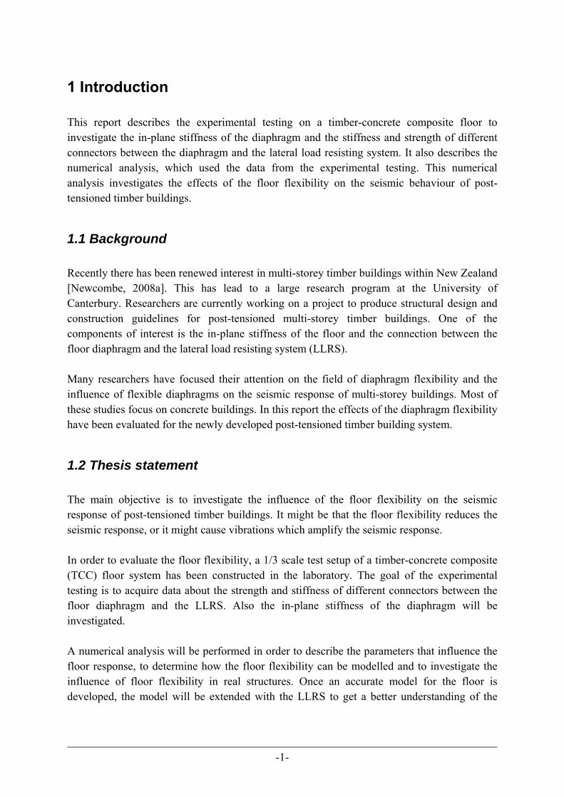
3.5 Loading The loading protocol used for testing was based on ISO CD 21581 [2007]. Even though the testing is performed on a floor slab and not a shear wall, this code provides a more extensive test protocol (especially at lower amplitudes) then EN 12512 [CEN, 2001]. For each test an ultimate displacement was assumed which determined the displacement increments. The maximum displacement for each test (except Test 2) was 20mm in order to get a good comparison between the different tests. Each displacement level during testing was cycled three times, although during some tests the higher displacement cycles were only performed twice, in order to save time. An example of a loading protocol is given in Figure 3.14.
-20
-15
-10
-5
0
5
10
15
20
0 500 1000 1500 2000 2500 3000 3500
Steps
Dis
plac
emen
t [m
m]
.
Figure 3.14 – Example loading protocol according to ISO CD 21581

-20-
3.6 Recycling After the testing was done the floor had to be demolished. All the different materials were separated and where possible recycled, as can be seen on Figure 3.15. The LVL joists can be used for other tests. The concrete will be used as hard fill.
Figure 3.15 – Recycling of the floor (clockwise: metal fasteners and brackets, LVL, plywood and concrete)

-21-
4 Results experimental testing A total of seven tests were performed, as shown in Table 4.1. Each test used a different kind of connection between the floor and the frame. The first test was performed by M. Newcombe and M. Le Heux [2008]. Chapter 4.1 is a summary of their results.
Test nr. Connection between Fasteners Size [mm] Amount Angle [°] 1 Timber-to-concrete Screws Ø5.3 – 75 10 90 2 Timber-to-concrete Screws Ø5.3 – 100 12 45 3 Timber-to-timber Screws Ø5.3 – 125 10 90 4 Timber-to-timber Nails Ø5.3 – 125 20 90 5 Timber-to-timber Screws Ø5.3 – 150 12 45 6 Timber-to-timber Screws Ø5.3 – 200 10 90 7 Diaphragm test *
* The last test was performed with 8 coach screws, Ø15 mm, and 6 steel angles to restrain the connection.
4.1 Test 1 – Timber-to-concrete, screws, 90°
Description
The first test was performed with a connection between the timber and the concrete. Ten coach screws, Ø5.3 – 75 mm, installed at a 90° angle with the timber frame were used.
Prediction
Previous full-scale research [Smith, 2008] showed that the bearing capacity of the concrete was the governing failure mode. The capacity of one connector was estimated at 6.8 kN with formulas given by EC 5 [CEN, 2004b]. The total capacity of all ten screws would be 68 kN.
Test results
The hysteresis loops in Figure 4.2 show how the floor behaved under the cyclic loading. The maximum force reached was 32 kN. From the larger displacement loops a residual force of 7 kN was a result of friction between the floor and the supports. The remaining 25 kN was resistance provided by the connectors. After taking away some timber and concrete around one of the connectors, see Figure 4.1, the failure mode could be seen. It was not the expected failure of the concrete, but instead, double hinge yielding in the screw took place.
Table 4.1 – Overview of connections per test
Figure 4.1 – Double yielding in the fastener [Le Heux, 2008]

-22-
The capacity of this failure mechanism can be estimated using the formulas given in Eurocode 5 for steel-to-timber connections. The thick steel plate analogy is used to simulate the screw being held in the concrete. This failure mode occurs at 2.8 kN per screw, see Appendix A, if the rope effect is not taken into account. This is higher than the results found in the test, 10 * 2.8 > 25 kN.
4.2 Test 2 – Timber-to-concrete, screws, 45°
Description
The second test was done to see how inclined screws would perform in the timber-to-concrete connection. A total of 12 coach screws, length of 100 mm, Ø5.3, were placed at a 45º angle with the timber framing, see Figure 4.3. This length of screws gave the same perpendicular depth in the timber as the screws used for Test 1.
Figure 4.2 – Hysteresis loops Test 1 [Le Heux, 2008]
Figure 4.3 – Timber-to-concrete connection with screws under a 45° angle

-23-
To speed up the testing sequence, a high strength grout (see Chapter 3.3.3) was used to fill the gap around the connectors that was necessary to remove the fasteners from the previous test.
Prediction
A paper by Kavaliauskas [2007] gives three formulas for possible failure modes in screws installed at an angle in the timber. These formulas are derived from Johansen’s yield theory. The governing failure mode (III) is double yielding in the screw, as shown in Figure 4.4, at a load of 12.4 kN. The problem however is that no information could be found about inclined screws when subjected to cyclic loading. All the available information was based on inclined screws in tension; while during cyclic loading compression also occurs. Therefore the assumption was made by us that only the screws under tension would contribute to the force transfer in the connections. This seemed reasonable since the stiffness of screws under tension is probably larger then under compression. But more research is needed in this area. The total capacity of the connectors is predicted to be 6 * 12.4 = 75 kN.
Test results
The failure mode was not in the screw and the timber but in the grout, as can be seen in Figure 4.5.
During this test, not only rigid body movement but also rotation of the floor diaphragm took place. This can be concluded from Figure 4.6. The dashed line is the movement of the ram, in the middle of the floor. A large variation in movement between the connections on the north and south side can be seen. This difference was caused by the movement of the reaction frame, which resulted in a rotation of the floor.
Figure 4.4 – Failure mode III [Kavaliauskas, 2007]
Figure 4.5 – Failure in the grout

-24-
Figure 4.7 shows the development of the hysteresis loops. Each graph shows three series of three displacement cycles. The first and second graphs show an elastic response from the connectors. The third and forth graph show a more ductile behaviour. Besides the rotation, there was also some movement between the timber frame and the steel reaction frame and in the steel reaction frame itself. Therefore not the total displacement of the floor, but the average displacement over the connections was used for the hysteresis data. This is why the 10mm displacement cycles (the last cycles in Figure 4.6) did not result in a 10mm displacement, but only 7mm, as can be seen in the last graph of Figure 4.7.
Figure 4.6 – Connection displacement for Test 2
Figure 4.7 – Hysteresis loops Test 2, 4 graphs with each three series of three displacement cycles

-25-
Figure 4.8 shows all the hysteresis loops in one graph and the backbone curve. This curve is the envelope that shows the maximum force which is reached for each displacement. During the test the maximum force reached was 79 kN. From the previous test it was concluded that approximately 7 kN was friction. This resulted in a shear force of 72 kN for all connectors, or 12 kN per connector (in tension). Calculations done after the fastener testing (see Appendix A) show that the screws would fail at 9 kN. But the failure in the grout indicated that this value was not reached. This shows that the screws in compression also were contributing to the load resisting behaviour of the system. The screws in compression should contribute at least for 50% of the capacity. So that each screw in tension resisted a force of 8 kN and the ones in compression 4 kN.
4.3 Test 3 – Timber-to-timber, screws, 90°
Description
After an earthquake it is difficult to repair a connection between the concrete layer and the timber floor. The concrete around the old connectors needs to be taken out; the connection needs to be replaced and new concrete or grout would need to be poured. This is not something which is desirable based on cost and building occupancy requirements. An alternative is a connection between the outer joist and the timber frame. These connections are easy to fabricate and easy to repair.
Figure 4.8 – Hysteresis loops Test 2

-26-
For this test ten 125 mm long Ø5.3 mm screws were used, placed as shown on Figure 4.9. Half of this length was threaded, so the threaded portion was at the interface between the frame and the joist. The screws were self-drilling.
Prediction
This connection was a fairly straight forward timber-to-timber connection, of which the capacity can be calculated utilizing formulas from Eurocode 5 [CEN, 2004b]. There are 6 different failure modes possible, see Figure 4.10. The calculated capacities are as follows:
a. 12.2 kN b. 7.6 kN c. 19.7 kN d. 6.9 kN e. 6.8 kN f. 3.9 kN
The rope effect was taken fully into account in these predictions. The expected failure mode was f; double yielding in the screw and bearing failure in the timber. So the total capacity of the 10 connectors was predicted at 39 kN.
Figure 4.9 – Connection Test 3
Figure 4.10 – Six failure modes according to EC5 [CEN, 2004b]

-27-
Test results
Figure 4.11 shows the remainder of the fastener. It was broken at two places, about 26 mm apart. So the prediction of the failure mode was correct. The maximum force reached during the test was 45 kN at a displacement of 6 mm, as can be seen on Figure 4.12. Again, approximately 7 kN was assumed for the friction, so the connectors resisted 38 kN. After the fastener testing the six failure modes were calculated again (see Appendix A). Without the rope effect the screws would fail at 2.9 kN, with the full rope effect the capacity would be 5.3 kN. From this it can be concluded that only a part of the rope effect can be taken into account for screws under cyclic loading.
4.4 Test 4 – Timber-to-timber, nails, 90°
Description
Nails were tested as an alternative to screws. Only nails installed at a 90° angle were tested, since the withdrawal capacity of nails is lower then that of screws. Therefore, Eurocode 5 limits the rope effect to 15% of the Johansen part for round nails, compared to 100% for screws. For this test 20 nails have been used. The nails had a 5.3 mm diameter and a length of 125 mm. The first 20 mm were predrilled to get a start for hammering in the nails.
Figure 4.11 –Failure of the fastener
Figure 4.12 – Hysteresis loops Test 3

-28-
Prediction
The same formulas as for Test 3 were used to calculate the capacity of the nails, except that the rope effect was limited to 15% of the connector capacity. The failure mode was still mode f; double yielding and bearing failure. The capacity of one nail was 2.25 kN, so in total a maximum force of 45 kN was expected.
Test results
The results of this test are shown in Figure 4.13. The maximum force resisted was 78 kN and was reached at a displacement of 14 mm. This hysteretic response shows that nails created a very ductile connection.
The maximum force was much higher then expected, which is probably caused by limiting the rope effect in the prediction. Table 4.2 shows the various capacities of the connection with different contributions of the rope effect. See Appendix A for the calculations. The connectors resisted a force of approximately 71 kN (78 kN minus 7 kN of friction). Similar to test 3, it can be seen that only a part of the rope effect can be taken into account. The 15% limit set by EC5 seems to be very conservative.
% rope effect Capacity per
connector [kN] Capacity all
connectors [kN] 0 2.5 50 15 2.9 58
100 4.0 80
Figure 4.13 – Hysteresis loops Test 4
Table 4.2 – Influence of the rope effect on the capacity

-29-
4.5 Test 5 – Timber-to-timber, screws, 45°
Description
A test of timber-to-timber connections with screws under a 45° angle is performed in order to get a good comparison between screws under a 45° and a 90° angle. Twelve screws with a length of 150 mm were used for this test.
Prediction
In a paper by Bejtka [2002] an adaptation of the Johansen’s yield theory for inclined screws is given. Three different failure modes are possible. The adapted form of double yielding is the governing failure mode and results in an estimated strength of 8.1 kN per screw in tension. The behaviour of inclined screws under cyclic loading is still not well known, as already mentioned in Chapter 4.2.2. Therefore the assumption was made again that the screws in compression did not contribute to the strength of the connection. The maximum force was predicted at 49 kN (6 times 8.1 kN).
Test results
Figure 4.14 shows the result of Test 5. The maximum force achieved was 61 kN, at a displacement of only 2 mm. Again, some rotation of the floor diaphragm was noticed during the test, but less than during Test 2.
Figure 4.14 – Hysteresis loops Test 5

-30-
After the test the screws were removed and, surprisingly, three of them (all in tension under positive displacement) had not broken. The screws had yielded, but the ultimate strength had not been reached. The failure was in the timber, as can be seen in Figure 4.15. This explains why the loops of the hysteresis graph are not symmetrical (between 4 and 12 mm) and why the last loops maintained a high resistance.
The calculations in Appendix A show that failure mode 2b (single yielding in the fastener and failure in the timber) and failure mode 3 (double yielding of the fastener) occur both at approximately 7 kN. This explains why two different failure mechanisms are seen. According to the assumption that only the screws in tension take up the force, the capacity would be 42 kN (6 times 7 kN). Figure 4.14 shows that a strength of 61 kN is reached, of which 7 kN is friction, so the connectors take up 55 kN. The difference of 13 kN is the contribution of the screws in compression. That would mean that they take up approximately 25% of the total force. After the screws were taken out, the 20 mm cycles were repeated. This was done to see how much friction there was in the system. The black line in Figure 4.16 shows the average result of this test. The increase of friction towards the end may be explained by the remainders of connectors from the previous tests. It was not possible to take the old connectors completely out since they were broken. This probably resulted in some resistance at larger displacements.
Figure 4.15 – Failure in the timber frame and the screw still fixed to the joist
Figure 4.16 – Hysteresis loops and friction loop Test 5

-31-
4.6 Test 6 – Timber-to-timber, long screws, 90°
Description
During Test 3 (timber-to-timber, screws, 90°) the screws broke in the threaded part. Test 6 was conducted to see if it made any difference if the yielding (and finally breaking) of the screws took place in the shank. This could give a more ductile connection, like with the nails. This time screws with a length of 200 mm, Ø5.3 mm and a threaded length of only 75 mm were used. These screws were self-drilling.
Prediction
The prediction was the same as for Test 3, so 39 kN.
Test results
Figure 4.17 shows the hysteresis loops of this test. The maximum force resisted was 35 kN at 4 mm displacement. The friction found after the previous test is also plotted in Figure 4.18. This explains why it seems that the strength is increasing towards the end (backbone is going up). But the difference between the maximum applied load (backbone) and the friction is actually decreasing. Figure 4.17 does not show the expected ductile behaviour. This is due to the high steel grade of the fasteners, which made them brittle, as is seen during the fastener testing.
Figure 4.17 – Hysteresis loops Test 6

-32-
Figure 4.18 – Hysteresis loops and friction loop Test 6

-33-
4.7 Test 7 – Diaphragm stiffness
Description
The final cyclic diaphragm test was performed in order to get information about the stiffness of the diaphragm. Previous testing, focused on retrofitting of existing buildings [Brignola, 2008], had been done on different kinds of timber floors. A TCC floor was one of the alternatives as a retrofit technique, but no testing had been done for the type of floor under investigation here. For this test the connections between the floor diaphragm and the LLRS had to be much stronger than during previous tests, to allow for a higher capacity of the hydraulic actuator to be reached. This was needed in order to get as much displacement as possible in the diaphragm and to determine the strength of the concrete diaphragm, instead of the strength of the connectors. Therefore eight Ø15 mm coach screws, placed between the outermost joist and the LLRS frame, and 6 steel angles, see Figure 4.19, were used to fix the floor to the frame.
The deformation of the diaphragm was measured at 5 places, 500 mm center to center, spread out over the width of the floor, as shown in Figure 3.3. The displacement of the connectors was measured with 4 linear pots, two at each side. The displacement of the whole system was measured with the rotary pot at the middle of the floor.
Test results
There are three deformation components to be considered when looking at floor system diaphragm test data, the movement in the reaction frame, the movement in the connections and the movement of the diaphragm. Figure 4.20 shows the hysteresis data for the whole
Figure 4.19 – Steel angles to fix the floor diaphragm

-34-
system. Figure 4.21 shows the hysteresis data of only the connections, and Figure 4.22 shows the hysteresis data of the diaphragm. Figure 4.23 shows the backbone curves of the displacement of all three components during the test. It can be seen that the displacement of the diaphragm was very small compared to the total displacement.
Figure 4.20 – Hysteresis loops of the whole system
Figure 4.21– Hysteresis loops of the connection

-35-
Zooming in on the stiffness of the diaphragm as in Figure 4.22, it can be seen that the diaphragm did not have the same stiffness in both loading directions. This may have been caused by an accident during construction, which resulted in a large crack (and probably some micro-cracks) on the side of the positive movement. During the 7 mm cycle a crack started to form in the middle of the floor, see Figure 4.26. From Figure 4.20 it can be seen that this was under a load of approximately 120 kN on the positive side and 150 kN on the negative side. Figure 4.22 shows a distinct change in the stiffness of the diaphragm at exactly these force levels. So, due to the cracking, the stiffness of the floor slab decreased significantly.
Figure 4.22 – Hysteresis loops and stiffness of the diaphragm
Figure 4.23 – Stiffness comparison of the diaphragm, the connection and the reaction frame
Cracked diaphragm
Cracked diaphragm
Uncracked diaphragm
Partially cracked diaphragm

-36-
The displacement at 5 locations on the diaphragm, at the peak displacement of some cycles, is shown in Figure 4.24. From these lines it can be seen that the diaphragm showed some bending and shear deformation, although the magnitude was fairly small.
During the test the concrete started to crack in the corners where it was fixed by the steel angles. A crack width of over 2 mm was recorded during the test, see Figure 4.25. The complete cracking pattern can be seen in Figure 4.26. In the corners a lot of cracks were formed due to the steel supports which resulted in tensile forces in the concrete. Also significant cracking could be seen around the top and bottom of the floor, which was from Test 2, due to the timber to concrete connections. A big flexural crack can be seen from left to right, which occurred during the final test at a displacement of 7mm.
Figure 4.24 – Displacement of the diaphragm
Figure 4.25 – Cracking of the concrete

-37-
Figure 4.26 – Complete cracking pattern in the concrete

-38-
5 Discussion and conclusions of experimental results This chapter discusses the results of the experimental testing and conclusions are drawn from the comparison between the tests. The strength and stiffness of the different connections are compared. Also the difference between screws and nails is discussed, as well as the effect of having the threaded part or the shank of a connector at the interface of the connection.
5.1 Connection strength Figure 5.1 shows the backbone curves from the timber-to-concrete (1 & 2) and timber-to-timber (3 & 5) tests with the screws. For easy comparison, the curves have been modified to show the result of only 10 fasteners per test (instead of 20 for the nails and 12 for the 45° connections). The maximum strength is also shown in Table 5.1. It can be seen that there is no significant difference in strength between timber-to-timber and timber-to-concrete connections. The timber-to-concrete connectors placed at a 45° angle were nearly twice as strong as the connectors at a 90° angle. This difference was not observed for the timber-to-timber connectors. The maximum force was reached at a displacement of around 2 mm if the connectors were installed at a 45° angle, compared to 5 mm if the connectors were installed at a 90° angle.
Test Angle [degrees] Maximum strength
(positive) [kN] Maximum strength
(negative) [kN] 1 – Timber-to-concrete 90 37 -33 2 – Timber-to-concrete 45 64 -64 3 – Timber-to-timber 90 45 -45 5 – Timber-to-timber 45 46 -50
Table 5.1 – Overview of maximum strength for timber-to-concrete and timber-to-timber connections
Figure 5.1 – Comparison between the maximum strength for the timber-to-concrete and timber-to-timber connections

-39-
5.2 Connection stiffness Figure 5.2 shows the same backbone curves as Figure 5.1. It can clearly be seen that the initial stiffness of the connectors installed at a 45° angle, 80 kN/mm, was four times as stiff compared to the connectors place at a 90° angle, 20 kN/mm.
5.3 Comparison between screws and nails Figure 5.3 shows the backbone curves for the tests with nails and screws installed at a 90° angle between the timber joist and the LLRS. The initial stiffness of both connectors is the same. The screws were a bit stronger than the nails, which was mainly caused by the difference in steel quality. The failure modes were the same, both showed double yielding. The displacement at which the connectors failed was quite different. The screws reached their maximum force at approximately 5 mm and the nails at approximately 14 mm of displacement. Clearly the nails exhibited much more ductile behaviour than the screws.
Figure 5.2 – Comparison between the stiffness for the timber-to-concrete and timber-to-timber connections
Figure 5.3 – Comparison between screws and nails as connectors

-40-
5.4 Comparison between thread and shank at connection interface The threaded section of the screw can influence the ductility of the connections as is shown in the testing of the fasteners in Section 3.4. Test 6 has been performed with long screws so that the yielding would take place in the shank. But the long screws used were very brittle, as can be seen in Table 3.4. Therefore, unlike the nails, they broke at a lower displacement and did not exhibit the desired ductile behaviour as can be seen in see Figure 5.3.
5.5 Diaphragm The stiffness of the diaphragm is largely dependent on the cracking in the concrete. The uncracked diaphragm showed a stiffness of approximately 4000 kN/mm. The cracked diaphragm showed a stiffness of approximately 300 kN/mm. It has to be noted that the displacements of especially the uncracked diaphragm were within 0.04 mm. The experimental stiffness value might not be very accurate due to irregularities in the test specimen, unconsidered effects like friction and the accuracy of the instrumentation at that level of displacement. The stiffness of a floor system consists of two parts, the stiffness of the floor slab and the stiffness of the connection between the floor slab and the LLRS. The range of stiffness of the connectors is from 20 to 80 kN/mm, as can be seen from Figure 5.2. Table 5.2 gives the influence of the diaphragm stiffness on the total stiffness of the floor. It is assumed that the stiffness of the connectors and the stiffness of the diaphragm can be modelled as serial springs, as is proposed by Brignola [2008].
Figure 5.4 – Comparison between fasteners with the thread and shank at the interface of the connection

-41-
Most flexible option Most stiff option Diaphragm stiffness 500 kN/mm (cracked) 4000 kN/mm (uncracked) Connector stiffness 20 kN/mm (90° angle) 80 kN/mm (45° angle)
Combined stiffness 11 1( ) 19.2 /
20 500kN mm−+ =
11 1( ) 78.4 /80 4000
kN mm−+ =
Influence of the diaphragm stiffness
19.2 20 100% 3.8%20
−× = −
78.4 80 100% 2.0%80
−× = −
The influence of the diaphragm stiffness is less than 4% in both options. So the in-plane floor stiffness of the floor used in this experiment can be modelled by only the connection stiffness. The diaphragm stiffness of the TCC floor used in this experiment can be neglected in the seismic design.
Table 5.2 – Influence of the diaphragm stiffness

-42-
5.6 Conclusions The experimental testing showed that there are major structural differences between the different connections which were tested. The timber-to-concrete connection with screws installed at a 45° angle was nearly twice as strong as the screws at a 90° angle. For the timber-to-timber connections the orientation did not seem to influence the strength of the connection. The displacement at maximum force was approximately 2 mm for the screws at a 45° angle, compared to 5 mm for the screws at a 90° angle and 14 mm for the nails. The stiffness of the connections with screws installed at a 45° angle was approximately 80 kN/mm. This was four times stiffer than the screws installed at a 90° angle. No difference in stiffness between the nails and the screws was found. The threaded part of the screws is influencing the ductility of the connectors. This is shown by the fastener testing. Making connections with the shank at the interface could result in a more ductile connection. But this could not be confirmed by the experimental testing. The rope effect which is used for the design of screwed connectors in EC5 can not be taken fully into account for screwed connections at a 90° angle under seismic (cyclic) loading. More research is needed in order to determine which part of the rope effect can be taken into account. There is not enough information available for the design of inclined screws under seismic loading. Only information on inclined screws under tension is available. A conservative design approach would be to neglect the strength of the screws in compression. The stiffness of the uncracked TCC floor diaphragm which was tested was approximately 4000 kN/mm. In a cracked state this reduces to approximately 300 kN/mm. For the floor used in this experimental test it can be concluded that the flexibility of the diaphragm can be neglected in comparison with the flexibility in the connectors.

-43-
6 Numerical analysis of a floor unit This chapter describes the first part of the numerical analysis, which has been performed to determine the effect of the floor flexibility on the seismic behaviour of multi-story timber buildings. The numerical model is described and the important parameters for the design are identified. Five designs with different slenderness ratios of the floor have been made. The design parameters for each design are calculated, and are used for a numerical time-history analysis with Ruaumoko [Carr, 2008]. The results from these analyses are discussed in the end of this chapter.
6.1 Introduction The goal of this part of the numerical analysis is to describe the components that influence the floor flexibility and to determine how the floor flexibility can be modelled. Therefore the LLRS is assumed rigid and only the stiffness of the diaphragm and the connectors is considered. In later stages (Chapter 7 and 8) of the analysis the influence of the floor flexibility on the global response of a structure will be looked at. The floor flexibility consists of three different parts, the deformation of the connectors, the shear deformation in the diaphragm and the flexural deformation in the diaphragm, as shown in Figure 6.1. In the experimental part it was already determined that, for the geometry considered, the flexibility of the diaphragm could be neglected.
6.2 Numerical Model Three different models have been made. The first model is a multi degree-of-freedom (MDOF) model, which represents a real floor system as closely as possible. The mass of the floor needs to be distributed to a number of points, since a distributed mass would result in infinite degrees of freedom in the model. Therefore the floor is represented as 8 beam elements, which is enough to get an accurate result [Spooner, 2008]. The connectors are
Figure 6.1 – Three floor deformation components

-44-
represented as springs with a linear stiffness. This is valid as long as the forces imposed on the connectors are not larger than the elastic limit. The second model is a single degree-of-freedom model, named ‘SDOF-1’ hereafter, which only takes the stiffness of the connectors into account. This model is made to determine if the influence of the diaphragm can be neglected completely. The third model, named ‘SDOF-2’ hereafter, is made to include the diaphragm stiffness by representing it as a spring. The stiffness of this spring will consist of the shear and flexural stiffness of the diaphragm. This stiffness will be combined with the connector stiffness according to Eq. 6.1. This model does include the diaphragm stiffness, but not the possibility of the development of higher modes of response. Other researchers [Fleischman and Farrow, 2001] shown that these higher modes of response can significantly influence the forces generated in the structure.
11 1eff
conn diaphragm
k
k k
=+
Eq 6.1
All the three models are shown in Figure 6.2. The nodes which represent the mass of the floor have thick lines. Movement is allowed in the x-direction but restricted in the y-direction. Rotation is only allowed for the nodes 2 to 10 in the MDOF model.
Figure 6.2 – Three numerical models

-45-
6.3 Design Parameters Two important parameters in the design are the depth and the length (the span) of the floor. These parameters determine the total area and thus the mass of the floor. This mass generates inertial forces when subjected to accelerations during an earthquake. These forces have to be transferred from the diaphragm into the LLRS. So the design of the connectors depends on the mass, and thus the floor depth and floor span. The ratio of the floor span (L) over the floor depth (D) is the aspect ratio (λ) of the floor. Five designs have been considered with different aspect ratios, as shown in Figure 6.3. The cross-section, the shear area and the second moment of inertia are calculated according to Eq. 6.2(a)-(c) and are shown in Table 6.1.
Design A [m2] As [m2] I [m4] A 1.26 1.05 34.02 B 1.26 1.05 34.02 C 0.42 0.35 1.26 D 0.56 0.47 2.99 E 0.42 0.35 1.26
Besides the two parameters mentioned above, there are also some parameters which stayed constant during the analysis. These are shown in Table 6.2. Also shown is a reference to a chapter where the parameter is discussed.
Figure 6.3 – Five designs with different aspect ratios
Table 6.1 – Overview section properties
3
56
112
s
A t D
A t D
I t D
= ×
= × ×
= × ×
Eq. 6.2(a) Eq. 6.2(b) Eq. 6.2(c)

-46-
Parameter Symbol Magnitude Chapter Thickness floor slab t 70 mm Modulus of elasticity of concrete E 28.000 kN/mm 6.4 Shear modulus of concrete G 11.000 kN/mm 6.4 Factor for cracked EI n 0.2 6.4 Floor mass W 3.3 kN/m2 6.5 Design Peak Ground Acceleration PGA 0.70 g 6.6 Floor Acceleration Magnification FAM 1 or 3 6.6 Connector yield strength fy 1000 N/mm2 6.6 Connector diameter d 10 mm 6.6 & 6.7
An overview of the design process which leads to the diaphragm stiffness can be seen in Figure 6.4. This figure also shows references to a chapter where the step of the design procedure is discussed. Figure 6.5 shows the design process for the calculation of the period of the connectors. This parameter will be used as the major variable in the presentation of the results.
Table 6.2 – Fixed design parameters
Figure 6.4 – Schematics of the calculations of the diaphragm stiffness

-47-
Figure 6.5 – Schematics of the calculations of the period of the connection

-48-
6.4 Stiffness of the diaphragm The stiffness of the diaphragm needs to be known for the SDOF-2 model. The diaphragm stiffness consists of two parts, the flexural and the shear stiffness. The experimental results from the diaphragm test will be used to determine these two stiffness values. The tested diaphragm will be idealized as a beam which is clamped at both ends, because the test rig prevented the ends from rotating. This idealization is shown in Figure 6.6.
12
18M Fl=
21
18M Fl=
The flexural stiffness of the diaphragm will follow from the deflection in the middle of the span. The values of θ can be expressed as the area underneath the M/EI line, as shown in Eq 6.3(a)–(c).
21
1 6
1 412 1881
M l FlEI EI
θ θ× ×
= = = × Eq. 6.3(a)
22
2 5
1 212 18
324
M l FlEI EI
θ θ× ×
= = = × Eq. 6.3(b)
22
3 4
3118
108
M l FlEI EI
θ θ×
= = = × Eq. 6.3(c)
The flexural deformation in the middle of the span can be described by Eq. 6.4.
1 2 323 11 154 54 12m l l lθ θ θδ = × − × − × Eq. 6.4
Figure 6.6 – Beam model of the diaphragm for determining the flexural stiffness

-49-
Eq. 6.4 together with Eq. 6.3 forms Eq. 6.5
3 3 3 31 23 1 11 1 1 581 54 324 54 108 12 1296m
Fl Fl Fl FlEI EI EI EI
δ = × − × − × = × Eq. 6.5
Figure 6.7 compares the result of Eq. 6.5 with two other loading cases. The deflection under the two point loads is less than the deflection under one point load, but more than the deflection under a distributed load.
3 31 0.0052192m
Fl FlEI EI
δ = × = ×
3 35 0.00381296m
Fl FlEI EI
δ = × = ×
4 31 0.0026
384mql FlEI EI
δ = × = ×
From Eq. 6.5 the flexural stiffness of the clamped beam can be derived as shown in Eq. 6.6.
3
3
5 1296 1296 5flex
Fl EIF k k kEI l
= ×δ = × × → = × Eq. 6.6
A similar derivation can be done for the shear stiffness, as shown in Figure 6.8 and Eq. 6.7 and Eq. 6.8.
1 2FV =
Figure 6.7 – Comparison of the deflection under three different loading configurations
Figure 6.8 – Beam model of the diaphragm for determining the shear stiffness

-50-
1 / 2 13 6m
s s
F FllGA GA
δ = × = Eq. 6.7
6
6s
shears
GAFlF k k kGA l
= × δ = × → = Eq. 6.8
Assuming that the flexural and shear deformation are independent, they can be combined according to Eq 6.9.
11 1diaphragm
flex shear
k
k k
=+
Eq. 6.9
The modulus of elasticity of the concrete is of big influence on both stiffness values. Therefore this value is calibrated using the results from the experimental testing. The concrete used in the experimental test had an average compressive strength of 35 Mpa [Le Heux, 2008]. Design standards give different formulas for the modulus of elasticity as can be seen in Eq. 6.10(a)–(c).
0.3
22 32 3200010
cmfE GPa MPa⎛ ⎞= ≈ =⎜ ⎟⎝ ⎠
[CEN, 2004a] Eq. 6.10(a)
'4700 28000cE f Mpa= ≈ [ACI Committee 318, 2005] Eq. 6.10(b)
'3320 6900 26500cE f MPa= + ≈ [Standards New Zealand, 2006] Eq. 6.10(c)
The value from the American Standard (ACI) has been chosen from these three results, since it is the median value. The modulus of rigidity is given by Eq. 6.11. 0.4 0.4*28000 11000G E MPa= = ≈ [Standards New Zealand, 2006] Eq. 6.11 The equations 6.6, 6.8 and 6.9 give the following stiffness values for the uncracked diaphragm:
15120 /
1680 /flex
shear
k kN mm
k kN mm
=
= 1512 /diaphragmk kN mm=
The stiffness of the tested diaphragm is shown in Figure 6.9. The initial, uncracked, stiffness is around 4000 kN/mm, while the cracked stiffness is approximately 300 kN/mm. The theoretical stiffness of 1500 kN/mm is in the range of the experimental value. It has to be

-51-
noted that the displacements of especially the uncracked diaphragm were very small. The experimental stiffness value might not be very accurate due to irregularities in the test specimen, unconsidered effects like friction and the accuracy of the instrumentation at that level of displacement.
The cracked diaphragm stiffness is used to determine the reduced E-modulus of the cracked concrete. A value of 0.2crackedE E= gives the following stiffness values:
3024 /
336 /flex
shear
k kN mm
k kN mm
=
= 302 /diaphragmk kN mm=
This is in good correspondence with the test result. The largest diaphragm displacement occurs with a cracked diaphragm, so that gives a worst case scenario. Also, it is likely that due to shrinkage or during an earthquake cracking will occur, so for the modelling the following values for the modulus of elasticity and the modulus of rigidity are assumed:
0.2 5600 0.2 2240
cracked
cracked
E E MpaG G Mpa
= == =
Eurocode 5 [CEN, 2004c] states that as a simple approach a reduced stiffness value of 40% of the uncracked stiffness may be taken. The value of 0.2 (20%) is again a conservative approach since a more flexible diaphragm is more likely to show larger displacements and accelerations. With these values it is possible to calculate the diaphragm stiffness for each of the five designs presented in Chapter 6.3. In a real building the floor mass, and thus the earthquake
Figure 6.9 – Experimental stiffness of the diaphragm
Cracked diaphragm
Cracked diaphragm
Uncracked diaphragm
Partially cracked diaphragm

-52-
forces generated by the floor are generally distributed along the floor. Also the assumption that the ends of the floor are clamped by the LLRS is not valid anymore. Figure 6.10 shows the idealisation of the floor diaphragm which is used for the numerical models. Eq. 6.12 and 6.13 are used to calculate the flexural and shear stiffness of the diaphragm.
3
3
5 384 384 5flex
Fl EIF k kEI l
δ = / = × → = × Eq. 6.12
2 8/
8s
shears
GAqlF k kGA l
δ = = → = Eq. 6.13
An overview of the flexural and shear stiffness and the combined diaphragm stiffness is shown in Table 6.3. These values are used for the SDOF-2 model. The MDOF model uses the derived modulus of elasticity and modulus of rigidity as properties of the beam elements.
Design kflex [kN/mm]
kshear [kN/mm]
kdiaphragm [kN/mm]
Flexural part [%]
Shear part [%]
A 67737 3136 2997 4 96 B 8467 1568 1323 16 84 C 2508 1045 738 29 71 D 743 697 360 48 52 E 313 523 196 63 38
Figure 6.10 – Idealization of the floor diaphragm for numerical models
Table 6.3 – Overview diaphragm stiffness

-53-
6.5 Floor mass The mass which needs to be taken into account is taken from the New Zealand standard [2004].
A previous design [Newcombe, 2008c] gives the following values: G = 2.4 kN/m2 Q = 3.0 kN/m2
2* 2.4 0.3*3.0 3.3 /W G Q kN m= + Ψ = + = For each of the 5 designs the mass per length and the total mass are shown in Table 6.4. The difference in span would result in a difference in permanent weight. This difference is neglected in the design.
Design Mass per length [kN/m]
Total mass [kN]
A 60 360 B 60 720 C 20 120 D 26 312 E 20 240
Table 6.4 – Overview floor mass

-54-
6.6 Design of the strength of the shear connectors The earthquake causes an acceleration of the ground. The maximum value is the called the Peak Ground Acceleration (PGA). This movement results in an acceleration of each floor of the building. The majority of mass in a building is the weight of the floors. Non-structural elements, often sensitive components, are attached to the floor, which makes the Peak Floor Acceleration (PFA) an important design parameter [Reinoso and Miranda, 2005]. Different design codes give different values for the PFA as a function of the design PGA. A lower design value and an upper design value are chosen in order to simplify the analysis. The lower limit is derived from the maximum of the International Building Code (IBC) [International Code Council., 2003] where the assumption is made that the floor undergoes a peak acceleration (PFA) equal to the peak ground acceleration (PGA), so PFA / PGA = 1. This ratio is called the Floor Acceleration Magnification (FAM). The IBC codes upper limit is found to be unconservative by many researchers [Fleischman and Farrow, 2001; Lee et al., 2007], so a lower value is not considered. The upper limit is derived from the New Zealand standard [2004] and inferred as a maximum for researchers [Fleischman and Farrow, 2001; Rivera, 2008] which results in a FAM of 3. The PGA is evaluated according to the New Zealand standard for a site in Wellington city, with soil class C and a return period of 1/500 years. This results in a PGA of 0.70g or 6.9 m/s2. Thus the lower limit of the PFA is 6.9 m/s2 and the upper limit 20.6 m/s2. Using Newton’s second law the upper and lower limit for the horizontal force generated by the floor for each design can be calculated assuming that the entire floor mass is accelerated. These values are shown in Table 6.5.
Design Floor mass [ton]
Lower limit [kN]
Upper limit [kN]
A 36 247 742 B 72 494 1483 C 12 82 247 D 32 220 659 E 24 165 494
An EC5 design has been made to determine the strength of a timber-to-timber connection for a 10 mm diameter coach screw with a yield-strength of 1000 N/mm2. Laboratory testing showed that there was not a significant difference in the strength of the different orientations of timber-to-timber connectors. Therefore only screws installed under a 90o angle are considered for the strength of the connectors.
Table 6.5 – Overview connector forces

-55-
A Eurocode 5 calculation similar to the one in Appendix A.3 is made. The results are shown in Table 6.6. Evaluation of the test results showed that the rope effect cannot be taken fully into account for cyclic loading. Therefore a design strength of 12 kN is chosen.
Failure mode
Strength without rope effect [kN]
Strength with rope effect [kN]
a 32.0 -- b 32.0 -- c 13.3 15.7 d 12.6 15.0 e 12.6 15.0 f 10.6 13.1
The number of connectors needed to resist the seismic loading is shown in Table 6.7. The numbers have been rounded off upwards to an even number, since the connectors need to be placed at both sides of the floor.
Design Lower limit [kN]
Upper limit [kN]
No. Connectors lower limit
No. Connectors upper limit
A 247 742 22 62 B 494 1483 42 124 C 82 247 8 22 D 220 659 20 56 E 165 494 14 42
Table 6.6 – Strength of screwed connection for 6 different failure modes
Table 6.7 – Overview number of connectors

-56-
6.7 Design of the stiffness of the shear connectors The laboratory testing gave us the stiffness of 5 mm diameter connectors. The derivation below shows how this can be scaled for 10 mm diameter connectors.
In Figure 6.11 it holds that in case of two identical timber spices:
1 2 0.5x x x= = × Eq. 6.14 Further, the yield moment can be determined as:
21 1 1( )(0.5 ) 0.5y h hM F a f d x x f d x= × = × × × = × × × Eq. 6.15
Eq. 6.15 can be rewritten for x1.
1
2 y
h
Mx
f d=
× Eq. 6.16
Eq. 6.14 and 6.16 result in Eq. 6.17.
1
22 2 y
h
Mx x
f d= × = ×
× Eq. 6.17
The yield moment depends on the diameter of the fastener as can be seen in Eq. 6.18.
3
0.86ydMy f= × Eq. 6.18
Figure 6.11 – Double yielding of fastener

-57-
Eq. 6.16 and 6.18 together form Eq. 6.19.
3 2
1
2 0.8 1.6 1.62 2 2 2
6 6 6y y y
h h h
f d f d fx x d
f d f f× × × × ×
= × = × = × = × ×× ×
Eq. 6.19
Further it can be seen from Figure 6.11 that:
~u x Eq. 6.20 From Eq. 6.19 and 6.20 follows Eq. 6.21.
~u d Eq. 6.21 So there is a linear dependence between the displacement in the connection and the diameter of the fastener. The same is valid for inclined timber-to-timber connections [Bejtka, 2002].
2 3
1,1
2 cos2 1
y y
h
M M dx x df d d d
× αβ= × →
+ β ×∼ ∼ ∼ Eq. 6.22
And also for inclined timber-to-concrete connections [Kavaliauskas, 2007].
3
22 sin( ) y y
h
M M dx t x df d t d d
= × × α →× ×
∼ ∼ ∼ Eq. 6.23
The shear force for this failure mode (double yielding) is given Eq. 6.24.
3 221.15 2v y hF M f d d d dβ= × × × × × =
1+ β∼ Eq. 6.24
So there is a quadratic dependence between the shear force over a connection and the diameter of the fastener. The stiffness of the connection can be calculated with Eq. 6.25.
2F dk du d
= =∼ Eq. 6.25
This shows that there is a linear dependence between the stiffness of the connection and the diameter of the fastener.

-58-
Laboratory testing showed that the stiffness of 10 ø 5mm fasteners was between 20 and 80 kN/mm (depending on the orientation), so 1 ø 5mm has a stiffness between 2 and 8 kN/mm. With the previous derivation it can be concluded that 1 ø 10mm fastener has a stiffness between 4 and 16 kN/mm. The different stiffness values for the five designs are shown in Table 6.8. A comparison with EC5, Eq 6.26, shows that the derived stiffness of the 10mm diameter 90o angle screw connection is lower then prescribed by EC5. This was also noticed by other researchers [Dias, 2005].
1.5 1.5600 10 6.4 /23 23
mser
dK kN mmρ × ×= = = Eq 6.26
Design No. Connectors lower limit
No. Connectors upper limit
Stiffness lower limit [kN/mm]
Stiffness upper limit [kN/mm]
A 22 62 88 992 B 42 124 168 1984 C 8 22 32 352 D 20 56 80 896 E 14 42 56 672
The five designs have each been modelled with a range of different stiffness values for the connectors. The period of natural vibration for the connectors (Tconn) has been calculated according to Eq. 6.27. The five different ranges of connector period turn out to be all between 0.02 and 0.20 seconds, which makes it a good parameter for comparison of the different designs.
2connconn
MTK
π= × Eq. 6.27
Table 6.8 – Overview of upper and lower values for the connector stiffness

-59-
6.8 Overview of Design Parameters Table 6.9 and 6.10 give an overview of the design parameters for each of the five designs.
Design Aspect ratio (λ) A [m2] As [m2] I [m4]
Mass per length [kN/m]
Total mass [kN]
A 0.33 1.26 1.05 34.02 60 360 B 0.66 1.26 1.05 34.02 60 720 C 1.00 0.42 0.35 1.26 20 120 D 1.50 0.56 0.47 2.99 26 312 E 2.00 0.42 0.35 1.26 20 240
Design kdiaphragm [kN/mm]
kconnector lower limit [kN/mm]
kconnector upper limit [kN/mm]
Tconn lower limit [s]
Tconn upper limit [s]
A 2997 88 992 0.127 0.038 B 1323 168 1984 0.130 0.038 C 738 32 352 0.122 0.037 D 360 80 896 0.124 0.037 E 196 56 672 0.130 0.038
Table 6.9 – Overview design parameters (1)
Table 6.10 – Overview design parameters (2)

-60-
6.9 Results Each of the 5 designs has been evaluated seven times with different values of the connector stiffness in Ruaumoko. Each time the model was subjected to 15 different earthquake records. Examples and explanation of the input for Ruaumoko can be found in Appendix B. The earthquake records are presented in Appendix C. The time step used for the analysis is 0.01 seconds. In this chapter the process of acquiring the results from the analysis output and a summary of the results is shown. Design E with the MDOF model is used as an example, as can be seen in Figure 6.12. The results per design are added in Appendix D.
6.9.1 Statistics
The response of a structure to 15 different earthquake records varies widely. Therefore the statistical variability needs to be considered in order to compare the different designs. For each design the Median and the 84th percentile (or +Sigma) values have been calculated from the data sets of the 15 earthquakes. The Median and +Sigma have been chosen over the Average and Standard Deviation because they are less sensitive to extreme values in a data range, which might occur if one of the structures collapses. The Median value is ‘the exponent of the mean of the natural log values’ of the data set, as shown in Eq. 6.25. The 84th percentile (Eq. 6.27) is the Median multiplied by the exponent of the dispersion (Eq. 6.26), where the dispersion is determined as the standard deviation of the natural log values of the data set [Chopra, 2008].
1
1 * ln( )N
ii
xNmedian e ==∑
Eq. 6.25
2
1
1 * [ln( ) ln( )]1
N
ii
dispersion x medianN =
= −− ∑ Eq. 6.26
* dispersionsigma median e+ = Eq. 6.27

-61-
6.9.2 Floor displacements
The floor displacement can be split up in two parts, the displacement in the connectors and the displacement in the diaphragm itself. The displacement over the connectors is equal to the displacement of Node 2 (or Node 10) of the model. The displacement of the diaphragm equals the displacement of Node 6 in the model minus the displacement of Node 2. The total floor displacement is the combined displacement of the connectors and the
diaphragm, so that equals the displacement of Node 6. All these displacements are taken relative to the displacement of the ground (Node 1 or Node 11). The results of the 15 different earthquakes have been evaluated as explained in Chapter 6.9.1. Figure 6.13 shows the Median results of the connector, diaphragm and floor displacement and the +Sigma results for the floor displacement. In the results of the analysis, which are shown in Appendix D, only the Median and +Sigma displacements of the floor are shown for the three different models.
From Chapter 6.7 follows an upper limit for the stiffness of the connectors, namely having inclined screws and a FAM factor of 3. This upper limit for the stiffness gives a lower limit for the period of the connectors. Also a lower limit for the stiffness, and thus an upper limit for the period, of the connectors is derived for straight screws and a FAM factor of 1. These limits are the design limits, which are shown by the grey lines on the graph in Figure 6.13.
Figure 6.12 – Comparing Design E with the complex model
Figure 6.13 – Displacements of Design E calculated with the complex model

-62-
The design range, which falls between those limits, can be split up in different sections, as shown in Figure 6.14. Inclined screws give a stiff connection (so a low period), putting them on the left side in the design range. The opposite is the case for the straight screws. The FAM factor of 1 results in a low design force and thus a low number of connectors. Hence the low stiffness and the high period, which puts them on the right side in the design range.
The displacement of the floor is compared for the three different models shown in Figure 6.2. This is done by dividing the displacement according to MDOF model by the displacement according to the SDOF models. An example of such a comparison can be seen in Figure 6.15. This figure shows that the SDOF-2 model captures the response of the MDOF model really well; the maximum difference in displacement is only 8%. The SDOF-1 model however varies significantly from the MDOF model for the stiff connectors. The displacement of the diaphragm stays nearly constant over the full design range, but the displacement of the connector increases with an increasing period. Therefore the influence of the diaphragm displacement is the largest at a small period.
Figure 6.14 – Specification of the design range
Figure 6.15 – Comparison of the floor displacement between the MDOF model and the SDOF models

-63-
6.9.3 Floor accelerations
In addition to the displacements, the accelerations of the floor have also been evaluated. The PFA is expressed as the number of units of gravity (‘g’) felt by the floor. Figure 6.16 shows the distribution of the maximum PFA, of one earthquake (record 1 in this case), over the 9 different nodes of the MDOF model. It can be seen that the middle of the floor has the largest PFA. It also shows that it is reasonable to make the simplification that the whole floor undergoes the same acceleration, since there is only a 5% difference between the outer nodes and the middle node.
The maximum PFA can be evaluated for every earthquake. This gives a maximum value for the floor during one earthquake, as can be seen on the first graph in Figure 6.17. The maximum values for the 15 earthquakes are shown in the second graph of Figure 6.17. The Median and +Sigma values are calculated with the formulas given in Chapter 6.9.1. These and the PGA values are shown as the horizontal lines in the graph. The PGA is 0.70g, as explained in Chapter 6.6. The Median value, considering Tconn = 0.02s, is 0.79g and the +Sigma value is 1.40g. This gives PFA / PGA ratios of 1.13 and 2.00. These ratios are calculated for each of the seven different values of connector periods. This is plotted in the third graph of Figure 6.17. Also the ratios 1 (IBC) and 3 (NZ1170.5) are shown, as they are used as the lower and upper limit for the connector design. In theory, inelastic behaviour will occur if the PFA exceeds the PGA. However, this is conservatively ignored (by doing a linear elastic analysis) in this part of the study because the inelastic behaviour will reduce the diaphragm response.
Figure 6.16 – PFA distribution over the floor
[g]

-64-
It can be seen that the PFA/PGA increases as the period of the connection increases. This higher floor acceleration is due to an increase in the acceleration spectrum, as can be seen in Figure 6.18. The insert shows the period range in which the connector design is situated. A rigid floor system would have an infinite stiffness and thus a zero period. This means that, for the models considered in this chapter, the floor is exactly following the ground motion, and thus gives a PFA/PGA ratio of one. The flexibility introduced by the connectors and the diaphragm results in a system with a
Figure 6.17 – Explanation of processing the floor accelerations
Figure 6.18 – Spectral acceleration graph
Peak Floor Acceleration EQ7
Median PFA = 0.79 PGA = 0.70
PFA/PGA = 1.13

-65-
period of vibration, which is unequal to zero. Therefore the floor system no longer follows the exact ground motion. Figure 6.19 shows this for the MDOF system of Design E under earthquake 3, for a time period of 1 second. Two different connectors are shown, the most stiff connection (Tconn = 0.020s) and most flexible connection (Tconn = 0.203s). Figure 6.20 shows the same as Figure 6.19, but for a longer time period. Also shown is the Design PGA value of 0.7. It can be seen that the connection with the 0.020s period of vibration is better capable of following the vibrations of the earthquake record and thus shows less amplification than the connection with the 0.203s period.
Figure 6.19 – Comparison of the earthquake acceleration and two different floor vibrations
Figure 6.20 – Comparison of the earthquake acceleration with the floor acceleration
Tconn = 0.020s Tconn = 0.203s
0.2s

-66-
6.10 Comparison of the results First the comparison is made between the MDOF model and the SDOF-1 model, which only models the connectors and not the diaphragm. Figure 6.21 shows that this model only gives a good result (Displmdof / Displsdof-1 ≈ 1) for Design C and Design A, which both have a span of only 6 meters. The displacement of Design B (λ=0.66) is surprisingly far off compared to Design C (λ=1). This would suggest that the span of the floor is more important than the aspect ratio, something which is also noted by Nakaki [2000]. The model is the most accurate for higher periods of the connectors. This is because a high period means a low stiffness of the connectors. The low stiffness results in a large displacement of the connectors. Therefore the influence of the diaphragm displacement on the total floor displacement reduces.
The same comparison can be made for the MDOF model and the SDOF-2 model, which models both, the connectors and the diaphragm, as a single spring. Figure 6.22 shows that
Figure 6.21 – Comparison of floor displacements of the MDOF model and SDOF-1 model
Figure 6.22 – Comparison of floor displacements of the MDOF model and SDOF-2 model

-67-
there is a good agreement with the MDOF model over the complete range of connector stiffness; the maximum error is only 9%. Therefore it is valid to conclude that the diaphragm can be modelled as a linear spring, with the stiffness as described in Chapter 6.7. There are no major higher order effects introduced by the movement of the diaphragm. This model has been shown to be sufficient for all the designs considered, but it means that the flexural and shear stiffness of the diaphragm need to be calculated. It should be noted that even though the SDOF-1 model does not match the results from the MDOF model very well, the actual differences in displacements is only a couple of millimetres. Figure 6.23 shows the diaphragm displacement as calculated with the MDOF model. It can be seen that for all the models the diaphragm displacement stays below 2 mm. Therefore in the next step of the analysis, when the LLRS is added, it is possible that the SDOF-1 model may be sufficient to capture the overall response.
Figure 6.24 and Figure 6.25 indicate that the peak floor accelerations have a similar trend as the floor displacements. The SDOF-1 model predicts the accelerations well for Design A and C, but gives up to a 60% difference for Design E. The SDOF-2 model gives a good prediction over the complete range of connector stiffness; the maximum error is 17%.
Figure 6.23 – Diaphragm displacement according to the MDOF model
Figure 6.24 – Comparison of peak floor acceleration between the MDOF model and SDOF-1 model

-68-
The ratio of the PFA over the PGA is shown for the 5 designs in Figure 6.26. This graph shows the Median and +Sigma values from the analysis with the MDOF model. The other two models give a similar graph. It can be seen that the lower design limit, which is the upper design limit according to IBC, would only be valid for a rigid diaphragm. A flexible diaphragm is likely to show a larger acceleration. Therefore, designing according to the IBC would significantly underestimate the diaphragm accelerations and result in inelastic deformation in the floor diaphragm. The upper design limit of PFA/PGA ratio of 3 is a safe upper limit for connections with a period of up to 0.13 seconds. The design limit for the period of the connectors is 0.13 seconds. Design E, with the most flexible diaphragm, has a larger PFA then Design A, with the stiffest diaphragm. But there is no clear relationship between the aspect ratio and the peak floor acceleration. Designs with straight connectors are more flexible and have a higher connection period. Therefore they introduce higher accelerations in the floor diaphragm. A stiffer connection, with inclined screws, lowers the connection period and thus lowers the PFA.
Figure 6.25 – Comparison of peak floor acceleration between MDOF model and SDOF-2 model
Figure 6.26 – PFA / PGA according to the MDOF model

-69-
6.11 Conclusions The floor flexibility consists of three different parts, the deformation of the connectors, the shear deformation in the diaphragm and the flexural deformation in the diaphragm. The numerical analysis showed that it is not necessary to model the diaphragms as several beam elements. The simplification to model it as a spring element is justified. The analysis did not show a clear relationship between the aspect ratio of the floor and the seismic response. The difference was clearer when comparing the different spans of the floor. The numerical analysis showed that for short spans (6 meter) over 80% of the displacements take place in the connectors. Therefore, with those short spans, the influence of the diaphragm can be neglected. It is also shown that neglecting the diaphragm flexibility does not significantly influence the peak floor accelerations. For larger spans (over 6 meter) and especially spans with a high aspect ratio, there is a significant (over 20%) influence of the diaphragm flexibility on the floor displacements and the floor accelerations. The diaphragm needs to be included in the model, which can be done as a spring. It must be noted that although the influence is significant, the absolute displacements in the diaphragm stay below 2 millimeters. The floor accelerations can be assumed constant along the length of the diaphragm. The flexible floor can lead to accelerations of up to 3 times the PGA. This indicates that a rigid floor diaphragm assumption in a design can severely underestimate the floor accelerations. A stiffer connection (e.g. inclined screws) between the LLRS and the floor results in lower floor accelerations then less stiff connections.

-70-
7 Numerical analysis of a single storey building In the previous chapter several models of the floor flexibility were developed. The next step in the analysis is to add the LLRS to the floor and to investigate the influence of the floor flexibility on the overall response of a single storey building. A displacement based design has been made to estimate the stiffness of the LLRS. Again, Ruaumoko has been used for the analysis with the same 15 earthquake records. The results from the analyses are discussed in the end of this chapter.
7.1 Introduction This second part of the numerical analysis focuses on a single storey building. This is done to get a better understanding of the interaction between the floor diaphragm and the LLRS. With this model it will be possible to determine when a floor can be assumed rigid and when the flexibility should be taken into account.
7.2 Numerical Model The three models made in the previous chapter are used again, but with an extra spring added to model the LLRS. A forth model is made which only models the LLRS. This is shown in Figure 7.1.
Figure 7.1 – The four numerical models

-71-
7.3 Design Parameters The previous chapter showed that the influence of the floor stiffness was the biggest for Design E (λ=2). Therefore only this design has been considered for the modelling of the single-storey building. Two different LLRS are analysed, a frame solution and a wall solution. They represent the boundaries of the range in which a possible real solution will be situated.
7.4 Stiffness of the LLRS A displacement based design (DBD) [Priestley et al., 2007] has been made in order to determine the stiffness of the LLRS which is needed for the numerical analysis. Firstly, a DBD is presented for a single storey building where a frame is used for the LLRS as shown in Figure 7.2. Step 1. Determine the design displacement, the
effective mass and the effective height (Figure 7.3). The target inter-storey drift level for a timber frame structure is 2%. The New Zealand standard [2004] gives an inter-storey drift limit of 2.5% for the ultimate limit state. With a storey height of 3.2 meter, this gives a target displacement, Δd = 64 mm. The mass of the floor is its weight times the area. The analysed structure has a floor depth of 6 meter and a span of 12 meter, giving a total area of 72m2. The weight per square meter is 3.3 kN/m2, resulting in a total mass of 240 kN or 24.5 ton. The weight of the frame is estimated at 10% of the weight of the floor, so 24 kN or 2.4 ton. Since it is only a single storey building, its effective mass, me, equals its total mass, so 26.9 ton.
The effective height, He, is approximately equal to the total height for the single storey building, so He = 3.2 meter.
Figure 7.2 – Single storey building with frame
Figure 7.3 – Equations for the target displacement, effective mass and effective height

-72-
Step 2. Calculate the equivalent viscous damping. The equivalent viscous damping, ζeq, consists of two parts, the elastic damping, ζel, and the hysteretic damping, ζhyst. The elastic damping is assumed 2% and the hysteretic damping is assumed 20% [Newcombe, 2008c]. This high hysteretic damping gives a higher period and thus a lower stiffness. This lower stiffness creates the worst case lower design limit. So ζeq = 22%. Step 3. Determine the effective period from the reduced design displacement spectrum. The design spectrum needs to be scaled by a scaling factor Req as defined in Eq. 7.1.
0.5 0.57 7 0.542 2 22eq
eq
R⎛ ⎞ ⎛ ⎞= = =⎜ ⎟ ⎜ ⎟⎜ ⎟+ ζ +⎝ ⎠⎝ ⎠
Eq. 7.1
The scaled displacement spectrum can be seen in Figure 7.4. The effective period, Te, can be determined as 1.0 seconds. Step 4. Obtain the equivalent lateral stiffness.
The equivalent lateral stiffness, Ke, is given by Eq. 7.2.
2 2
2 2
4 4 26.9 1058 /1.00
ee
e
mK kN mT
π π× ×= = = Eq. 7.2
Step 5. Determine the base shear. The base shear, Vb, is given by Eq. 7.3
1058 0.064 68b e dV K kN= × Δ = × = Eq. 7.3 Step 6. Distribute the base shear up the structure. Since there is only a single-storey, the entire shear force is distributed to the one floor. So F1 = 68 kN. In Ruaumoko the hysteretic damping is conservately ignored since it will reduce the seismic response. In order to be able to compare the results of the numerical analysis with the DBD the target displacement needs to be back calculated according to the displacement spectrum belonging to 2% damping (instead of 22%), as shown in Figure 7.5. This calculation gives a design displacement of 156 mm. The corresponding base shear is 165 kN.
Figure 7.4 – The 5% and the scaled displacement spectrum
Figure 7.5 – The 5% and the scaled displacement spectrum

-73-
The same DBD calculation is done for a wall structure. The steps are summarized below. Step 1. The target inter-storey drift level for a timber wall structure is 1%, so Δd = 32 mm The mass of the wall is assumed to be 20% of the mass of the floor, so me = 29.4 ton He = 3.2 meter. Step 2. ζeq = 2%. No hysteretic damping is assumed here, which means a lower period and thus a higher stiffness. This is done to get the upper design limit. Step 3.
1.32eqR =
Te = 0.29 seconds. Step 4.
14157 /eK kN m= Step 5.
453bV kN= Step 6. F1 = 453 kN

-74-
7.5 Results A similar analysis as for the floor system (Chapter 6) has been performed for the single-storey building. The results are split in two parts. First the results from the single storey building with a frame as LLRS are presented and secondly the results from the model with the wall as LLRS.
7.5.1 Frame
The displacement can be split up into three parts, the displacement of the LLRS, the displacement of the connection and the displacement of the diaphragm. Figure 7.6 shows these displacement values for the MDOF floor model. It can clearly be seen that the displacement of the LLRS is much larger then the other components.
Figure 7.7 gives the Median and +Sigma displacement for all the four models. Also the calculated target displacement from the DBD is shown. The rigid floor model is only calculated once, since it does not model the connectors. Therefore there is no actual period of the connection. Hence, the displacement of the rigid floor model is constant over the entire range of connector period.
Figure 7.6 – Displacements of single storey building with frame as LLRS according to the complex model

-75-
Figure 7.7 shows that the displacements of the MDOF, the SDOF-1 and the SDOF-2 floor model are nearly the same. This can also be seen from Figure 7.8, where the ratio between these three models is nearly equal to 1. The rigid floor model is giving very good results at lower periods of the connectors, due to the limited influence of the connector displacement. For the higher periods of the connectors the rigid floor model is in the design range maximum 2% off.
Figure 7.7 – Comparison of floor displacements of single storey building with frame as LLRS
Figure 7.8 – Further comparison of displacements of single storey building with frame as LLRS
Figure 7.9 – Comparison of floor accelerations of single storey building with frame as LLRS

-76-
The floor accelerations are nearly constant for all the different values of connector stiffness, as can be seen in Figure 7.9. This means that the connector stiffness does not influence the floor accelerations for a single storey building with a frame as LLRS. This can be explained by looking at the period of the structure, simplified as a SDOF. The period of the LLRS is approximate 1.0 seconds, as calculated in the DBD. The equivalent stiffness of the LLRS and the connectors combined varies between 0.95 and 0.97 seconds as can be see in Eq. 7.5 and 7.6.
1 1 1.007 / 0.971 1 1 11.053 23
eff eff
LLRS conn
k kN mm T s
k k
= = = → =+ +
Eq. 7.5
1 1 1.052 / 0.951 1 1 11.053 2320
eff eff
LLRS conn
k kN mm T s
k k
= = = → =+ +
Eq. 7.6
This shows that the connectors hardly influence the period of the structure, and thus do not influence the floor accelerations. The Median shear force in the LLRS is shown in Figure 7.10. The force is nearly constant since the floor accelerations are also constant. The figure shows that the MDOF floor model gives a smaller shear force in the LLRS then the SDOF floor models and the rigid floor model. The shear force is higher than the design force according to the DBD due to the PFA being higher than the PGA
Figure 7.10 – Comparison of Median shear force of single storey building with frame as LLRS

-77-
7.5.2 Wall
The design with the wall as LLRS is much stiffer than the design with the frame. Therefore the displacement of the LLRS is much less and the influence of the flexible floor is larger. This can be seen in Figure 7.11 and Figure 7.12. Other researchers [Nakaki, 2000] also came to this conclusion when looking at precast concrete structures.
Figure 7.12 and Figure 7.13 show that the SDOF floor models describe the displacements accurately in comparison to the MDOF model. The rigid floor model shows an error of up to 23%.
Figure 7.11 – Displacements of single storey building with wall as LLRS according to the complex model
Figure 7.12 – Comparison of floor displacements of single storey building with wall as LLRS
Figure 7.13 – Further comparison of displacements of single storey building with wall as LLRS

-78-
The MDOF model gives the floor displacements and the rigid model gives the LLRS displacement, as shown in Figure 7.14. These values can be used to determine if the diaphragm can model assumed stiff according to different building codes as described in Chapter 2.4.1. In order to make the assumption that the diaphragm is rigid the New Zealand standard and the IBC state that ufloor ≤ ullrs. This is the case for the all the values of Tconn as can be seen in Figure 7.14. The Eurocode states that ufloor ≤ 10% * ullrs, it can be seen that this is only the case for Tconn < 0.055 seconds. Thus according to the Eurocode the flexibility of the floor should be taken into account for the design of this structure for Tconn > 0.055 seconds. This fits well with the results of Figure 7.13, which show that the rigid floor model gives more than a 10% difference with the MDOF model.
The accelerations are shown in Figure 7.15. Again, the SDOF floor models are accurate, but the rigid floor model is not. The accelerations are decreasing with the increasing period. This can be explained by looking at the effective period of the total structure.
1 1 8.8 / 0.331 1 1 114.2 23
eff eff
LLRS conn
k kN mm T s
k k
= = = → =+ +
1 1 14.1 / 0.261 1 1 114.2 2320
eff eff
LLRS conn
k kN mm T s
k k
= = = → =+ +
This time the connector stiffness is influencing the effective period of the structure. A comparison with the spectral acceleration spectra, as shown in Figure 7.16 shows the period range of the wall structure. The decline in the acceleration is exactly in the period range of the structure. Figure 7.15 shows that the Median PFA is twice the PGA. This is nearly double that of the frame structure. The spectral acceleration graph, Figure 7.16, shows that for a structure with a period of around 1 second (the frame structure), the design acceleration will be nearly half of the design acceleration for a structure with a period of 0.3 seconds. A rigid floor assumption,
Figure 7.14 – Comparison diaphragm flexibility with different code requirements
rigid (EC) flexible (EC)
-79-
in which case the connectors will be designed for a maximum of one PGA, will severely underestimate the floor accelerations. It can be seen that a design of the connectors for a FAM of 3 is much more realistic.
Figure 7.17 shows the median shear forces. They show an analogous result as the floor accelerations. The design target, F = 453kN, corresponds well with the median shear forces.
Figure 7.15 – Comparison of floor accelerations of single storey building with wall as LLRS
Figure 7.16 – Spectral acceleration graph
Figure 7.17 – Comparison of median shear force of single storey building with wall as LLRS
Frame
Wall

-80-
7.6 Conclusions This chapter showed that for a single storey structure with a low stiffness of the LLRS, like a frame, the influence of the diaphragm flexibility on the seismic design is negligible. The floor diaphragm and the connectors are much stiffer than the LLRS and thus hardly influence displacements, accelerations and shear forces. For a single storey with a stiff LLRS, like a wall, there is a significant influence of the floor flexibility. For very stiff connectors (inclined screws and FAM = 3) the floor diaphragm can be assumed rigid, as is also stated in the Eurocode. For all other connectors, the flexibility of the floor needs to be taken into account. Only taking the flexibility of the connectors into account is sufficient for an accurate result. Neglecting the floor flexibility can lead to an underestimation of the displacements of up to 23%. This increased displacement can lead to higher demands on gravity columns. It also leads to an underestimation of the floor accelerations, which can be up to twice the PGA (median results) and three times the PGA (+Sigma results). The Eurocode definition of a flexible diaphragm is much stricter, but seems to be more accurate than the definition provided in the New Zealand standard or the IBC.

-81-
8 Numerical analysis of a multi-storey building The last step in the numerical analysis is to model a multi-storey building. This chapter describes the model and the results of the analysis. A short overview of the displacement based design is given, since it is used for the Ruaumoko model and to determine the strength of the connectors.
8.1 Introduction A six storey post-tensioned building, shown in Figure 8.1, has been analysed in order to investigate the difference in seismic response between a model with flexible floor diaphragms and a model with a rigid floor diaphragm.
The analysis has been run three times, for a 1/50, 1/500 and a 1/2500 year earthquake. The design spectrum scale factor, according to the New Zealand Standard [2004], is 0.5, 1.0 and 1.8 respectively.
Figure 8.1 – 6 Storey building, artist impression, typical floor plan and connection detail [Newcombe, 2008b; Smith, 2008]

-82-
8.2 Displacement Based Design A displacement based design (DBD) has been performed [Newcombe, 2008c] for a six storey frame building for a 1/500 year earthquake. The calculations showed that the building has an effective period of 2.4 seconds at a design drift of 2%. This results in a design acceleration of 0.188g, as is shown in Figure 8.2. The other parameters and results of the DBD are shown in Table 8.1. The results from this design have been used to determine the strength of the connectors in the analysis.
Storey Height [m]
Mass (per frame)
[kN] Displacement
[m] Horizontal force
(per frame) [kN]
Shear force (per frame)
[kN]
Moments (per frame)
[kNm] Drift [%]
6 22.8 1229 0.36 482 482 1583 1.13% 5 19.0 1300 0.31 311 793 1302 1.30% 4 15.2 1300 0.27 262 1054 1733 1.48% 3 11.4 1300 0.21 206 1260 2071 1.65% 2 7.6 1300 0.15 144 1404 2308 1.83% 1 3.8 1300 0.08 75 1480 2432 2.00% 0 0.0 - 0.00 - 1480 3382 -
Figure 8.2 – Spectral acceleration for DBD
Table 8.1 – Results DBD for 6 storey building

-83-
8.3 Numerical Model The building is 6 storeys with an interstorey height of 3.8 meter and 5 bays of 7 meters long. Figure 8.3 shows how the mass of the building is modelled for the rigid floor model and for the flexible floor model. All the nodes on a floor are constrained to the same displacement in the horizontal direction, except for the nodes with the floor mass in the flexible model.
The frame represents a 2D model of one of the frames of the building shown in Figure 8.1. The building is a prototype design for the newly developed building system. Post-tensioning, together with energy dissipaters, create a ‘hybrid’ system which results in energy dissipating connections with self-centring capacity. This is incorporated in the model using rotational springs at the connections, as shown in Figure 8.3. Some typical sections are shown in Figure 8.4. The model uses a constant damping of 2% for the first and third mode shape. Gravity loads are applied to every node of the frame.
Figure 8.3 – 6 Storey building model with rigid floor and flexible floor assumption
Figure 8.4 – Typical sections of beams and columns

-84-
8.4 Design Parameters For this study, the main design parameters are the properties of the spring element which models the floor deformations. As shown in Chapter 7, the floor system for a frame building can be modelled with just the stiffness of the connectors to get a good prediction of the results. This time the spring is not a linear element, but the hysteresis data from the laboratory testing of the straight timber-to-timber screws (Test 3) has been used. The required strength of the connectors is determined using the upper limit of the IBC, which is 1 PGA. This results in a horizontal force of 482 kN. This is then amplified by an overstrength factor of 1.3 as described in several building codes (Chapter 2.4.2.) and by Gardiner et al. [2008]. The result is a design force of Fd = 625 kN. The hysteresis loops have been scaled according to the principles derived in Chapter 6.6 and 6.7. The hysteresis loops and the backbone curve are shown in Figure 8.5. The initial stiffness is 342000 kN/m, the yield displacement is 2 mm and the displacement at the ultimate force is 10 mm. This hysteresis data has been used for all three different earthquake intensities.
Figure 8.5 – Hysteresis loops used to model the properties of the connectors

-85-
8.5 Results The analysis has been run under the same 15 earthquakes as the other analysis. This time the analysis has been done with a time step of 0.001 seconds. The results are presented as the Median and +Sigma values. A complete overview of the results can be found in Appendix E.
8.5.1 – Drifts and displacements
The analysis gives the displacement of every point of the structure at every time step of the analysis. The maximum displacement at the floor closest to the effective height (which is around the 4th floor) has been selected, and the corresponding displacement profile, see Figure 8.6, is extracted for every earthquake. The inter-storey drift levels are used to show the deflection per floor. They are defined as the inter-storey deflection divided by the storey height, as shown in Figure 8.6. The absolute maximum drift levels of each storey of the frame are extracted from the analysis results. These maxima do not have to occur at the same time and thus may not be at the maximum displacement.
Figure 8.7 shows the Median frame deflections of the two models at the three different limit states. It can be seen that the different modelling of the floor (rigid or flexible) hardly influences the displacement profile. The displacement according to the DBD fits well with the 1/500 year event displacements; the maximum difference is only 20 mm.
Figure 8.6 – Derivation of the deflections (u) and inter-storey drift levels (D) for the 6 storey building
Figure 8.7 – Frame deflections at three different earthquake intensities for the 6 storey building

-86-
Figure 8.8 shows the displacement of the six stories over the duration of the earthquake. The displacements are from the third earthquake record and scaled for the 1/500 year event. The insert shows the peak displacements.
The maximum drift levels are shown in Figure 8.9. They show an increasing difference between the rigid and flexible floor levels for the stronger earthquakes. The flexible floor reduces the maximum drift as the level of inelasticity increases. This is because more energy is absorbed by the inelastic deformation of the floor.
The displacement based design, which is for a 1/500 year event, gives a good prediction of the drifts at the lower levels. At the higher levels the drifts are underestimated since the displacement based design does not take higher modes of vibration into account. These higher
Figure 8.8 – Frame deflections of the 6 stories under the third earthquake record
Figure 8.9 –Inter-storey drifts at three limit states for the 6 storey building

-87-
mode effects cause additional drifts mainly at the top levels of up to 0.4%. It is not expected that the DBD drift profile will match the 1/500 year EQ results, but rather that a uniform rotational demand (of 2% in this case) is achieved up the height of the structure [Priestley et al., 2007]. The scaling of the 1/500 year earthquakes is twice that of the 1/50 year earthquakes. The drift levels are scaled accordingly since the response is mostly elastic. The 1/2500 year earthquakes are 1.8 times the 1/500 year earthquakes. But the drift levels are increasing by a factor of 2.2. This is due to the inelastic behaviour which occurs during the 1/2500 year earthquakes, which reduces the effective stiffness of the frame system and thus increases the displacements.
8.5.2 – Interstorey shear forces and moments
The shear forces and moments are evaluated for every storey. They are summed at each instant for the 6 columns, as shown in Figure 8.10, and then the maxim value is taken. This can be represented by Equation 8.1 and 8.2.
[ ]6
1( ) , where ( ) ( )i
iV MAX V t V t V t
=
= = ∑ Eq. 8.1
[ ]6
1( ) , where ( ) ( )i
iM MAX M t M t M t
=
= = ∑ Eq. 8.2
The shear force per floor is constant since there is no horizontal loading on the structure between the storeys. The moments are linear across the height of the storey. Therefore the moments are evaluated at the top and bottom of each column. Figure 8.11 shows the shear force distribution over the height of the building. Figure 8.12 shows the moment distribution over the height of the building. The forces and moments of the flexible floor model show the same trend as the drifts, nearly the same at low earthquake intensity and lower at higher intensity earthquakes.
Figure 8.10 –Derivation of the shear force and bending moments for the 6 storey building

-88-
Figure 8.11 – Comparison of shear forces for the 6 storey building
Figure 8.12 – Comparison of bending moments for the 6 storey building

-89-
8.5.3 – Floor Accelerations
The peak floor acceleration is a key engineering design parameter for the response of a multi-storey structure to an earthquake. The floor acceleration is strongly dependent on the earthquake intensity. However, it is unclear in this case which intensity measure is most appropriate to show the amplification of the floor acceleration. It is chosen here to represent the floor accelerations as the ratio of the PFA over the PGA of the corresponding earthquake. This is the most appropriate for (near) rigid diaphragms [Bradley et al., 2008]. This makes that the floor accelerations are all relative to the actual ground acceleration, and thus 1 at ground level, as is shown in Figure 8.13. This figure shows that the 1/50 year event generates relatively large accelerations in the structure, while for the 1/2500 year event the accelerations are mainly less than the ground acceleration. Hence, inelasticity in the floor connectors (see the next paragraph) results in a reduction of the floor accelerations.
Figure 8.13 – Peak floor acceleration over the peak ground acceleration for the 6 storey building

-90-
8.5.4 – Connectors
The flexible model allows investigating of the forces and displacement over the connectors between the floor diaphragm and the LLRS. Figure 8.14 shows the displacement over the connectors in the top floor under the third earthquake, scaled for a 1/500 year event. The connector displacements exceed 2mm, which is the yield limit, but it stays well within the 10 mm, so there is no failure of the connectors. This can also be seen from the hysteresis loops belonging to the connection, which is shown in Figure 8.15.
The maximum displacement and corresponding force at each level under each earthquake are examined and plotted in Figure 8.16 to 8.18. It can be seen that under the 1/50 year earthquake the force in the connectors is below the design value of Fd = 625kN. This results in an elastic response, which explains why the displacements, drifts, accelerations, shear forces and moments are the same as for the rigid model. Under the 1/500 year earthquake the force in the connectors is larger then the yield force, but not as high as the ultimate force. So the structure stays intact, but has damage in the connectors. During the 1/2500 year earthquake the ultimate force is exceeded in some floors. Ten floors showed displacements over 40mm, which is not shown on the graph. This means that the connectors are broken and possible collapse of the structure occurs.
Figure 8.14 – Connector displacement at top floor under the third earthquake record
Figure 8.15 – Hysteresis loops of the connector at top level under the third earthquake record

-91-
Figure 8.16 – Connector displacement vs. Connector Force for 1/50 year earthquake
Figure 8.17 – Connector displacement vs. Connector Force for 1/500 year earthquake
Figure 8.18 – Connector displacement vs. Connector Force for 1/2500 year earthquake

-92-
8.5.5 - Acceleration Response Spectra
The design ground acceleration spectrum is used to determine the seismic response of a SDOF representation of a structure. In the previous chapters it was concluded that the floor flexibility could be idealized as a spring, with the stiffness of the connectors, attached to a single mass which represents the mass of the floor. This idealization gives a SDOF system. Therefore the response of the flexible floor can be evaluated with the help of a floor acceleration spectrum. The difference with the design ground acceleration spectrum is that the floor is not directly connected to the ground. So the floor does not experience the ground motion, but a motion which is filtered by the structure. This motion varies on each level of the structure. Figure 8.19 shows three graphs show the spectral acceleration at each level in the structure. Also shown are several periods, which are listed in Table 8.2. The first, second and third natural periods of the structure follow from the numerical analysis. The period of the connectors is calculated with Eq. 6.27 where M is the mass of one floor and Kconn is the initial stiffness of the connectors.
Description Period [s] First natural period 1.53 Second natural period 0.50 Third natural period 0.26 Connector period 0.12
Table 8.2 – Overview of periods

-93-
Figure 8.19 – Floor acceleration spectra at the levels 1 & 2, 3 & 4 and 5 & 6 of the building

-94-
The first three normal modes of vibration are shown in Figure 8.20. The mode shapes have been multiplied by the percentage of the effective mass that is associated with each mode shape. These percentages are 82%, 11% and 4% respectively. It can be seen that the first mode is dominant and that the influence of the third mode is only minor.
The first natural period of the structure is 1.53 seconds. The graphs in Figure 8.19 show a distinct spike in the spectral acceleration near this period. Another distinct spike can be seen close to the second natural period of 0.50 seconds and close to the third natural period of 0.26 seconds. Figure 8.21 shows the peak values of these two spikes divided by the ground acceleration for each level. It can be seen that these spikes correspond with the first, second and third mode of vibration. The second period response seconds shows little amplification at the 4th and 5th level, which is characteristic for the second mode of response. The peak value of 4 means that a SDOF system with a period of 1.6 seconds, attached to the sixth floor, has an acceleration of 4 times the ground design acceleration for the same SDOF system. However, it is demonstrated in Chapter 6, that the period of the connectors is much less.
Figure 8.20 – Three normal modes of vibration
Figure 8.21 – Floor acceleration magnifications

-95-
The spectral acceleration graphs give the response of a SDOF system which would be attached to the frame of the structure at each level. This is exactly how the floor has been idealised as shown in Chapter 7. The period of the connectors, which represent the floor, is also shown in Figure 8.20. It can be seen that there are no major differences in the spectral acceleration of the floor motion at the period of the connectors. Therefore the floor connectors can be designed according to the design spectral acceleration of the ground motion with minor inaccuracies. In general it can be concluded that the design spectral acceleration can be used for the design as long as the period of the floor is not near the first, second or third period of the structure. This can also be seen in Figure 7.15 and 7.16, where the floor accelerations follow the ground accelerations. Therefore, although it is appropriate to design the floor diaphragm according to the design acceleration spectrum for the ground motion for frames, it may not be the case for walls. The increased stiffness, and thus lower period, of inclined screws might make a difference for the seismic response of multi-storey wall structures. More investigation is needed in that area.

-96-
8.6 Conclusions From the previous analysis it can be concluded that the influence of the floor flexibility on the seismic response of a multi-storey post-tensioned timber building with a frame as LLRS is small. The extra displacement in the floors is negligible compared to the displacement in the LLRS. Only under major earthquakes, where the connectors between the floor diaphragm and the LLRS show a ductile behaviour, there is a reduction in the seismic response. This means that neglecting the influence of the diaphragm stiffness is a conservative approach. The median floor accelerations can be up to a factor 1.5 higher then the PGA. The top floor of the structure shows a severe increase in accelerations. The influence of the floor flexibility is only apparent if the connectors start yielding, which is the case for the 1/500 and 1/2500 year earthquake. The inelasticity in the floor connectors reduces the floor accelerations. The factor of 1.5 times the PGA is lower compared to the factor of 2, which was found for the wall structure in Chapter 7.5.2. The inelastic modelling in this chapter results in a lower seismic response than the elastic modelling. This was expected since the inelasticity leads to energy dissipation which decreases the seismic response. The design of the connectors between the LLRS and the floor can be done with the help of the design spectral acceleration, as long as the period of the floor is not near the first, second or third period of the structure. This is the case for the six storey frame structure which has been used in this chapter. But it is questionable whether this is the case for a structure with a wall as LLRS. In that case the stiffness of the connectors can make a difference.

-97-
9 Conclusions The influence of the floor flexibility on the seismic response of post-tensioned timber buildings is small. In most cases neglecting the floor flexibility is a conservative approach for the structural design of the building. Only for structures with a stiff LLRS (like a wall) and flexible connectors there can be an amplification of the displacements. In that case it is sufficient to include only the flexibility of the connectors. Including the flexibility of the floor diaphragm is not required. Table 9.1 gives an overview of the different analyses which have been performed in this report and how the floor flexibility can be modelled under different options. The experimental testing showed that the stiffness of connections between the diaphragm and the LLRS with inclined screws, 80 kN/mm, were approximately four times stiffer than connections with straight screws, 20 kN/mm. The strength of the timber-to-concrete connection with inclined screws was nearly double the strength of the same connection with straight screws. This difference was not observed for the timber-to-timber connections. The experimental testing showed that the rope effect can not be taken fully into account for the estimation of the strength of the connectors under cyclic loading. It is recommended that the design spectral acceleration is used for the design of the connectors between the floor diaphragm and the LLRS. This predicts the floor accelerations more accurately than a design using the PGA. Only the stiffness of the connectors needs to be taken into account for the determination of the period of vibration of the floor system. If a detailed analysis of the floor unit is needed, then for short spans the floor flexibility can be described using just the stiffness of the connectors. For long spans (> 6m), two serial springs can be used, one with the stiffness of the connectors and one with the flexural and shear stiffness of the diaphragm.
Type of analysis Options Modelling of floor flexibility
Multi-storey (6) building - LLRS = frame Rigid floor - LLRS = wall - inclined screws Rigid floor (*) - straight screws Connectors (*) Single-storey building - LLRS = frame Rigid floor - LLRS = wall - inclined screws Rigid floor - straight screws Connectors Detailed floor analysis - small span ( < 6m) Connectors
- large span ( > 6m) Connectors and floor diaphragm
* = more research needed in this area
Table 9.1 – Overview of how the floor flexibility can be modelled

-98-
10 Recommendations for further research The use of inclined screws in timber-to-timber and timber-to-concrete connections seems very promising due to the high initial stiffness. But very little information is available about the behaviour of such a joint under cyclic loading. More research could result in a better understanding of the strength and stiffness of the fasteners in tension and compression. More research is needed in order to determine which part of the rope effect of timber-to-timber and timber-to-concrete connections can be taken into account for estimating the strength of such a connection under seismic loading. Due to time constraints only a 2D numerical analysis of a 6 storey building with frames as LLRS was performed. A 2D analysis of a 6 storey structure with walls as LLRS is needed to evaluate the possible amplification which can occur when the period of the second mode of vibration is close to the period of the connectors. A 3D numerical analysis of different multi-storey timber buildings could be made to validate the conclusions made in this report.

-99-
11 References ACI Committee 318 [2005]. "Building code requirements for structural concrete and
commentary (ACI 318M-05)". American Concrete Institute, Farmington Hills, Mich., 436.
ASTM [2003]. "Standard Test Method for Determining Bending Yield Moment of Nails". F1575-03, A. International, ed.
Bejtka, I., Blaß H. J. [2002]. "Joints with inclined screws." CIB Working commision W18 - Timber structures, Meeting 35, Kyoto, Japan.
Bradley, B. A., Dhakal, R. P., Curbinovski, M., and MacRae, G. A. [2008]. "Prediction of spatially distributed seismic demands in structures". 14th World Conference on Earthquake Engineering, Beijing, China, 9.
Brignola, A., Podestà, S., Pampanin, S. [2008]. "In-plane stiffness of wooden floor". NZSEE Conference, Wairakei, New Zealand.
Buchanan, A. H. [2007]. Timber Design Guide, New Zealand Timber Industry Federation, Wellington, N.Z.
Buchanan, A. H., Deam, B. L., Fragiacomo, M., Pampanin, S., and Palermo, A. [2008]. "Multi-Storey Prestressed Timber Buildings in New Zealand." Structural Engineering International, 18,2, 166-173.
Carr, A. J. [2008]. "Ruaumoko". University of Canterbury, Christchurch, New Zealand.
CEN [2001]. "Timber structures - Test methods - Cyclic testing of joints made with mechanical fasteners". EN 12512, Brussels, Belgium, 13.
CEN [2004a]. "Eurocode 2 : Design of concrete structures - Part 1-1: General rules and rules for buildings". EN1991-1-1:2004 (E), European Committee for Standardization, ed., Brussels, Belgium, 225.
CEN [2004b]. "Eurocode 5 : Design of timber structures - Part 1-1: General - Common rules and rules for buildings". EN1995-1-1:2004 (E), European Committee for Standardization, ed., Brussels, Belgium, ii, 123.
CEN [2004c]. "Eurocode 5 : Design of timber structures - Part 2: Bridges". EN1995-2:2004 (E), European Committee for Standardization, ed., Brussels, Belgium, 29.
CEN [2004d]. "Eurocode 8 : Design of structures for earthquake resistance - Part 1: General rules, seismic actions and rules for buildings". EN1998-1:2004 (E), European Committee for Standardization, ed., Brussels, Belgium, 229.

-100-
CEN [2006]. "Timber structures - Calculation of characteristic 5-percentile values and acceptance criteria for a sample". EN 14358, Brussels, Belgium, 8.
Chopra, A. K. [2008]. Dynamics of structures : theory and applications to earthquake engineering, Prentice Hall, Upper Saddle River, NJ.
Deam, B. L., Fragiacomo, M., Buchanan, A. H. [2007]. "Connections for composite concrete slab and LVL flooring systems." Materials and Structures (2008), 41, 495-507.
Dias, A. M. P. G. [2005]. "Mechanical behaviour of timber-concrete joints", PhD Thesis, Faculty of Civil Engineering and Geosciences, Delft University of Technology, Delft, The Netherlands.
Fleischman, R. B., and Farrow, K. T. [2001]. "Dynamic behavior of perimeter lateral-system structures with flexible diaphragms." Earthquake Engineering & Structural Dynamics, 30,5, 745-763.
Gardiner, D. R., Bull, D. K., and Carr, A. J. [2008]. "Internal forces of concrete floor diaphragms in multi-storey buildings". NZSEE Conference, Wairakei, New Zealand.
International Code Council. [2003]. International building code, The Council, Falls Church, Va.
ISO [2007]. "Timber structures - Static and cyclic lateral load test method for shear walls". CD 21581, Geneva, Switzerland, 12.
Iverson, J. K., and Hawkins, N. M. [1994]. "Performance of precast/prestressed concrete building structures during Northridge earthquake." PCI journal, 39,2, 38-55.
Kavaliauskas, S., Kazimieras Kvedaras, A., Valiūnas, B. [2007]. "Mechanical behaviour of timber-to-concrete connections with inclined screws." Journal of Civil Engineering and Management, Vol XIII,No 3.
Le Heux, M. [2008]. "Floor Diaphragm Flexibility in Timber Buildings", Third Professional Year Project, Department of Civil Engineering, University of Canterbury, Christchurch, New Zealand.
Lee, H. J., Kuchma, D., and Aschheim, M. A. [2007]. "Strength-based design of flexible diaphragms in low-rise structures subjected to earthquake loading." Engineering Structures, 29,7, 1277-1295.
Linden, M. v. d. [1999]. "Timber-concrete composite floor systems", PhD Thesis, Faculty of Civil Engineering and Geosciences, Delft University Press, Delft, The Netherlands.
Lukaszewska, E., Johnsson, H., Fragiacomo, M. [2007]. "Performance of connections for prefabricated timber–concrete composite floors." Materials and Structures.

-101-
Nakaki, S. D. [2000]. Design guidelines for precast and cast-in-place concrete diaphragms, Earthquake Engineering Research Institute, Oakland, California.
Newcombe, M. P. [2008a]. "Design Procedures and Numerical Analysis for Multi-storey Post-tensioned Timber Buildings", PhD Proposal, Department of Civil Engineering,, Canterbury University.
Newcombe, M. P. [2008b]. "Seismic Design of Post-Tensioned Timber Frames". 14th World Conference in Earthquake Engineering, Beijing, China.
Newcombe, M. P., Pampanin, S., Buchanan, A.H., and Palermo, A. [2008c]. "Seismic Design of Multi-storey Post-Tensioned Timber Buildings", Masters Thesis, University of Pavia, Pavia, Italy.
Palermo, A., Pampanin, S., and Buchanan, A. H. [2006]. "Experimental Investigations on LVL seismic resistant wall and frame subassemblies." First European Conference on Earthquake Engineering and Seismology, Geneva, Switzerland
Palermo, A., Pampanin, S., Buchanan, A. H., and Newcombe, M. P. [2005]. "Seismic design of multi-storey buildings using Laminated Veneer Lumber (LVL)". NZSEE Conference, Wairakei Resort, Taupo, New Zealand.
Priestley, M. J. N., Calvi, G. M., and Kowalsky, M. J. [2007]. Displacement-based seismic design of structures, IUSS PRESS, Pavia, Italy.
Reinoso, E., and Miranda, E. [2005]. "Estimation of floor acceleration demands in high-rise buildings during earthquakes." The Structural Design of Tall and Special Buildings, 14,2.
Rivera, A. J. [2008]. "On the development of seismic design forces for flexbile floor diaphragms in rc wall buildings", PhD Presentation, ROSE School, Pavia, Italy.
Seibold, E. [2004]. "Feasibility Study for Composite Concrete/timber Floor Systems Using Laminated Veneer Lumber in New Zealand", Department of Civil Engineering, University of Canterbury, Christchurch, New Zealand.
Sika Ltd [2008]. "Sika® Grout GP". New Zealand.
Smith, T. [2008]. "Feasibility of Multi Storey Post Tensioned Timber Buildings: Detailing, Cost and Construction", Masters Thesis, Department of Civil Engineering, University of Canterbury, New Zealand.
Spooner, M. S. [2008]. "Quantifying the Dynamic Response of Flexible Floor Diaphragms", Third Professional Year Project, Department of Civil Engineering, University of Canterbury, Christchurch, New Zealand.

-102-
Standards New Zealand [1993]. "3063 - Timber structures standard". Standards New Zealand, Wellington, New Zealand.
Standards New Zealand [2004]. "1170.5 - Structural Design Actions Part 5: Earthquake Actions - New Zealand". Standards New Zealand, Wellington, New Zealand.
Standards New Zealand [2006]. "3061 - Concrete structures standard". Standards New Zealand, Wellington, New Zealand.
Yeoh, E. C., Fragiacomo, M., Buchanan, A. H., Crews, K., Haskell, J., and Deam, B. L. [2008]. "Development of semi-prefabricated timber-concrete composite floors in Australasia". 10th World Conference of Timber Engineering, Miyazaki, Japan, 8.

-103-
Appendix A – Calculations connection strength

-104-

-105-
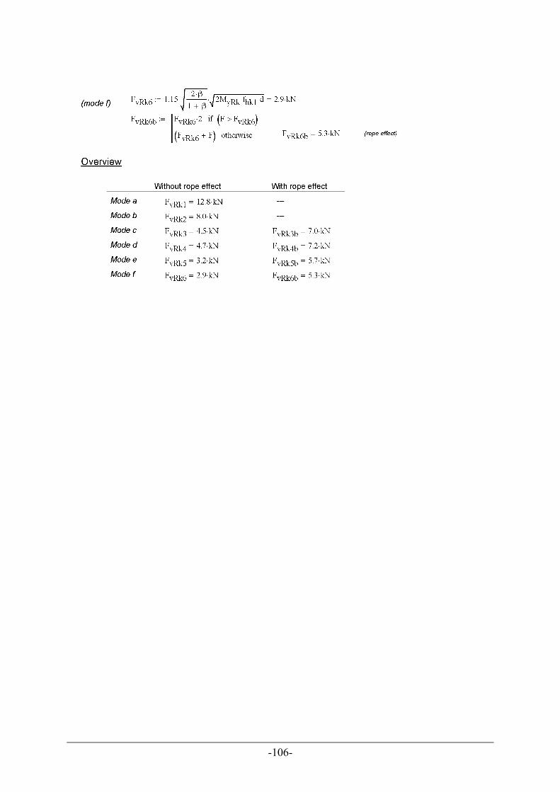
-106-

-107-
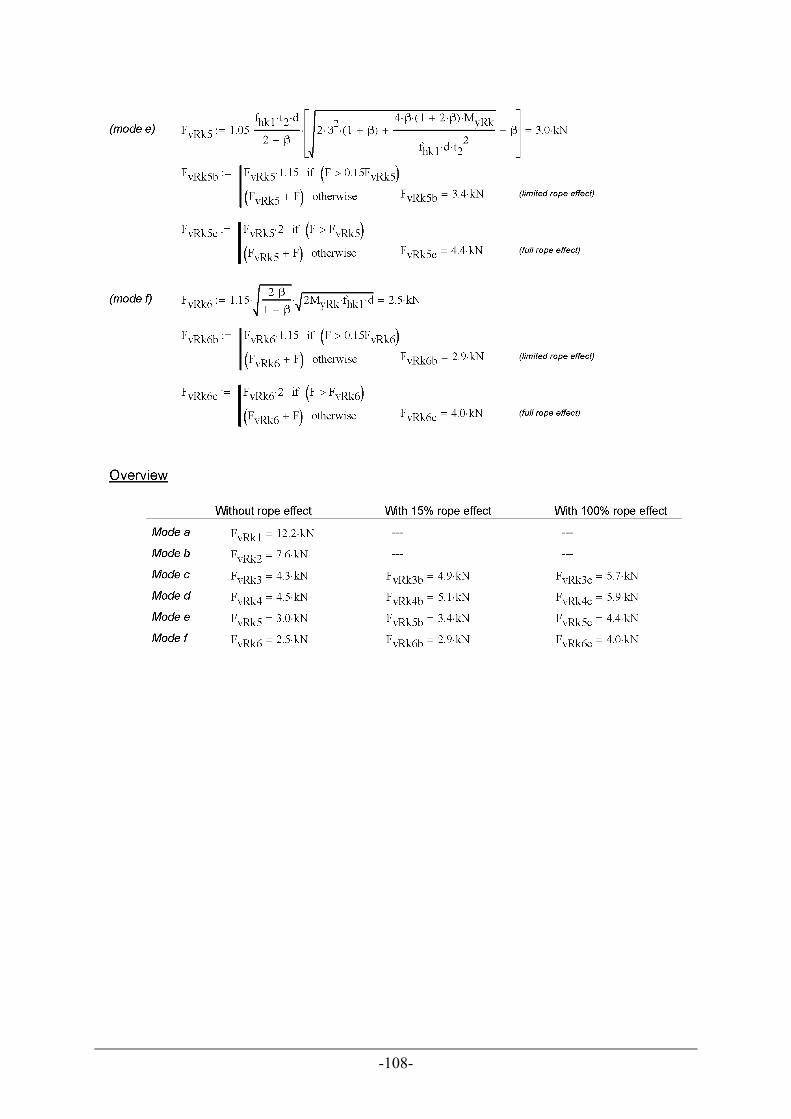
-108-

-109-

-110-

-111-
Appendix B – Ruaumoko Frame Files First an overview of the main settings for the numerical analysis is given. Secondly, three files are shown which form the input for Ruaumoko. These files are modelling Design E, with the highest connector stiffness, under the first earthquake record.
B.1 – Program settings
Principle Analysis Options IPANAL 2 Dynamic time-history using newmark constant average acceleration IFMT 0 Binary post-processor file with extension .RES IPLAS 1 In-elastic Time-history Analysis only IPCONM 0 Lumped mass matrix used in Time-history ICTYPE 6 Rayleigh Damping with Tangent damping matrix as Secant damping matrix IPVERT 0 X-direction earthquake only INLGEO 2 P-Delta effects included IPNF 0 Modal analysis is carried out after the static analysis IZERO 0 All zero output is omitted ORTHO 0 Mode shape orthogonality check not carried out IMODE 0 Householder QR eigenvalue algorithm used (Default) Frame Control Parameters NNP 11 Number of nodals points in the structure NMEM 10 Number of members in the structure NTYPE 2 Number of different cross-section in the section table M 5 Number of mode shapes required to be printed in the modal analysis MODE1 1 The mode number at which the first damping ratio is applied MODE2 2 The mode number at which the second damping ratio is applied GRAV 9.81 The acceleration of gravity C1 2 The percentage of critical damping at mode MODE1 C2 2 The percentage of critical damping at mode MODE2 DT 0.01 The time-step TIME 50 The length of time-history to be run FACTOR 1.2 A scale factor applied to the time-history input Output Intervals and Plotting Control Parameters KP 0 Time-history output suppressed KPA 10 Post-processor DYNAPLOT output every k time-steps KPLOT 10 Plastic hinges plotted every k time-steps JOUT 0 No used any longer, supply 0

-112-
DSTORT 1 No used any longer, supply 1 DFACT 1 Displacement multiplying scale factor for on-screen graphics XMAX 1 Maximum X displacement for use in the on-screen graphics YMAX 1 Maximum Y displacement for use in the on-screen graphics NLEVEL 1 Number of levels for computed inter-storey drifts, i.e. number of storeys+1 NUP 2 Vertical axis for inter-storey drifts, 1=X axis or 2=Y axis. IRESID 0 Residual displacements and forces not output KDUMP 0 Mass and stiffness matrices output suppressed Iteration Control and Wave Velocities MAXIT 10 Maximum number of cycles of Newton-Raphson iteration per Time-step MAXCIT 5 Maximum number of cycles of iteration/solution step for damping models FTEST 0.0001 Norm of the out of balance force vector realtive to the incremental force vector for the Newton-Raphson or damping iteration. The value is the square of the iteration tolerance required.i.e. 0.0001 implies a tolerance of 1% in the residual vector. WAVEX 0 Wave velocity of propogstion in the x-direction (if=0.0 taken as infinitive) WAVEY 0 Wave velocity of propogstion in the y-direction (if=0.0 taken as infinitive) THETA 0 Angle of earthquake X and Y directions to the structure X and Y directions DXMAX 1.5 X displacement to terminate analysis DYMAX 0 Y displacement to terminate analysis D 0 Travelling wave dispersion factor, 0.0 implies no dispesion OMEGA 0 Earthquake characteristic frequency (radians/second) used for dispersion F 0 Scale factor for dispersion

-113-
B.2 – MDOF model
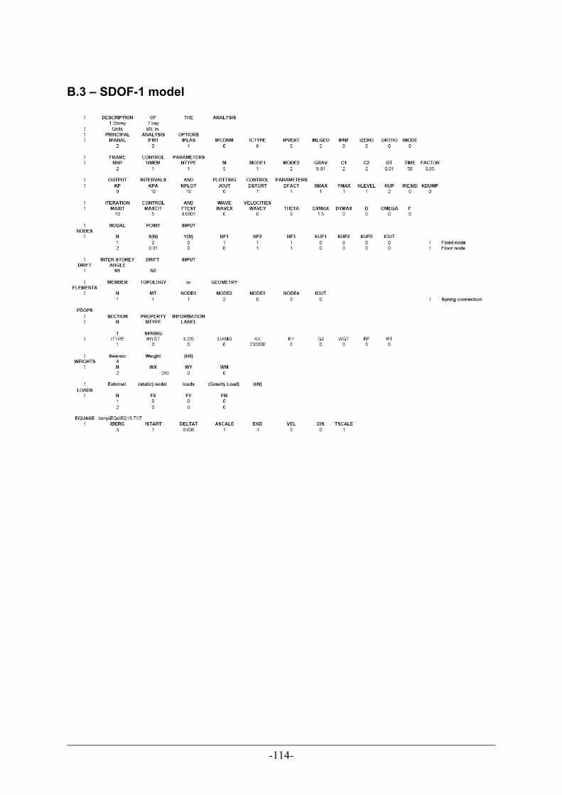
-114-
B.3 – SDOF-1 model

-115-
B.4 – SDOF-2 model

-116-
Appendix C – Earthquake records Using NZS1170.5 earthquake spectra:
• Soil type C • Sp = 1.0 • Risk factor = 1.0 for 1/500y and 1.8 for 1/2500y. • Wellington city zonation, z = 0.4 • Distance to fault = >20km • Damping for design spectrum: 2%.
The earthquake spectra and target spectra are shown below for 2% damping and are scaled over a period range of 0.64s (0.4T1) to 3.0s (the corner period > 1.3 T1).
1 1.5 2 2.5 30
0.2
0.4
0.6
0.8
1
1.2
Period (s)
Spec
tral A
ccel
erat
ion:
k1*
Sa (g
) Target SpectraAverage
Note, the scaling limit according to NZS1170.5 (between 0.3 and 3) is exceeded for 3 EQs.
EQ Near field
or far field
Location Dist. to source
[km] Time step Scale Factor
1/500y 1/2500y1 NF Northridge, Los Angeles Dam 5.92 0.005 1.2 2.16 2 NF Norhtridge, Sylmar - Olive view Med Ctr 5.3 0.005 0.6 1.08 3 FF Tabas, Iran (BOS_L1) 26.1 0.02 4.49 8.08 4 FF Nothridge, N Hollywood – Coldwater Can 14.6 0.005 2.18 3.92 5 FF Northridge, Canoga Park – Topanga Clan 15.8 0.005 1.82 3.28 6 N/A Artificial EQ (generated using SPECTRA) - 0.01 1.22 2.20 7 FF Superstition Hills, El Centro Imp. Co. Cent 13.9 0.005 2.16 3.89 8 FF Superstition Hills, Plaster City 21 0.005 4.49 8.08 9 FF Cape Mendocino, Fortuna Fortuna Blvd 23.6 0.005 2.68 4.82
10 NF Loma Prieta, Los Gatos Pres Center 3.88 0.005 0.55 0.99 11 FF Northridge, LA – N Faring Rd 23.9 0.005 3.22 5.80 12 NF Chi Chi, TCU068 9.96 0.005 0.56 1.01 13 FF Landers, Yemo Fire Station 24.9 0.005 2.65 4.77 14 FF Loma Prieta, Hollister Diff. Army 25.8 0.005 1.29 2.32 15 NF Tabas, Iran 2 0.005 0.85 1.53

-117-
Earthquake record 1 Earthquake record 2
Earthquake record 3 Earthquake record 4
Earthquake record 5 Earthquake record 6
Earthquake record 7 Earthquake record 8
Earthquake record 9 Earthquake record 10

-118-
Earthquake record 11 Earthquake record 12
Earthquake record 13 Earthquake record 14
Earthquake record 15

-119-
Appendix D – Graphs numerical analysis floor unit
D.1 - Results Design A
The next figures show the results for the first design, with λ = 0.33.

-120-
D.2 - Results Design B
The next figures show the results for the second design, with λ = 0.66.

-121-
D.3 - Results Design C
The next figures show the results for the third design, with λ = 1.00.

-122-
D.4 - Results Design D
The next figures show the results for the forth design, with λ = 1.50.

-123-
D.5 - Results Design E
The next figures show the results for the fifth design, with λ = 2.00.

-124-
Appendix E – Graphs numerical analysis multi-storey building
E.1 – 1/50 year event

-125-

-126-
E.2 – 1/500 year event

-127-

-128-
E.3 – 1/2500 year event

-129-